Determination of the refractive-index profile of light-focusingrods: accuracy of a method using Interphako interferencemicroscopy

Yasuji Ohtsuka and Yasuhiro Koike

Two analysis procedures to determine the refractive-index profile using Interphako interference microscopyare compared for accuracy: (I) expressing the. profile as a five-nomial equation (proposed previously byOhtsuka and Shimizu); (II) considering ray bending due to the index gradient and using Abel inversion (pro-posed by ga et al.). Computer simulations indicate that the errors of both procedures are comparable ex-cept for index mismatching between the specimen periphery (np) and immersion oil (n2) where Analysis (I)is more accurate than Analysis (II). The partial splitting method is more practicable than total splitting fora rodlike specimen. In addition, the improved partial splitting procedure facilitates reduction of error. Theindex profiles of the two selected light-focusing plastic rods (LFR) were calculated with these two proceduresin various conditions. The correlation between resulting profiles and measuring conditions agreed with thesimulations. It is concluded that Analysis (I) is preferable to Analysis (II) when n F n and that the im-proved partial splitting procedure is a practicable method for determining the index profile of a LFR.

1. IntroductionWe reported that a light-focusing plastic fiber (LFF)l

could be fabricated by the continuous heat-drawingprocess of a light-focusing plastic rod (LFR) preparedby the photocopolymerization process. 2 To determinethe refractive-index profiles of a LFR and a LFF, whichare both graded-index types, we have proposed thetransverse interferometric technique3 using the shearingmethod of Interphako 4 interference microscopy as anondestructive method. Here the light beam travelsthrough the specimen in a straight line, and the radialindex distribution of the specimen is expressed with aneighth-order polynomial. For the bending of raystraced through the LFR, Iga et al. proposed a nonde-structive method5 using the same interferometrictechnique. This easy method seemed convenient forcontinuous measurement along the center axis in asample compared with the destructive ones such as re-flection,6 near field,7 and interferometric slab.8 Re-cently other nondestructive methods such as lightscattering, 9 diffraction,10"1 focusing,12 fast Fouriertransform,' 3 and refracted ray tracing' 4 have beenproposed.

The authors are with Keio University, Faculty of Engineering,Department of Applied Chemistry, 3-14-1 Hiyoshi, Kokoku-ku, Yo-kohama-shi, 223, Japan.

Received 20 February 1980.0003-6935/80/162866-07$00.50/0.© 1980 Optical Society of America.

In this paper we compare, by computer simulation,our technique with Iga's for accuracy. The effect of themismatch in refractive indices between the specimenperiphery (np) and the matching oil (n2) is examined,because it is difficult to match refractive index n2 of thematching liquid with np, especially when the sample rodhas a graded-index distribution up to the peripherywithout any homogeneous cladding region. We alsocompare the index distributions of representativespecimens resulting from the two methods.

II. Fringe ShapeThe interference fringes analyzed were obtained by

the following procedure, which is the same as in Ref. 3:The cylindrical specimen in a glass cell was immersedin the liquid whose refractive index n2 was close to indexnp at the periphery of the LFR. Glass cell G was placedon stage St as shown in Fig. 1. The light beam tra-versing the LFR was divided into two by prism PrI.One beam was displaced at a distance Ayp perpendic-ular to the light axis by rotary wedge RW (shearingdevice) and then recombined with the other beam byprism PrII.

When shearing distance Ayp is longer than diameter2rp of the rod specimen, the two individual images ofthe specimen are completely separated, and we canobtain an ordinary Mach-Zehnder interference pattern(total splitting) such as shown in Fig. 2(a). On the otherhand, when the sample images are slightly sheared (Ayp<< 2rp), an overlapped image pattern is observed such

2866 APPLIED OPTICS / Vol. 19, No. 16 / 15 August 1980

EP

Pr- \

, .PAYP

RW

OL G

St - - 1

CL

-- t

Fig. 1. Primary elements for the shearing method of Interphakointerference microscopy: Lt, light source; SI, slit; CL, condenser lens;St, stage; G, glass cell; S, sample; OL, object lens; PrI, beam splittingprism; RW, rotary wedge; PrI, beam combining prism; EP, eyepiece;

Ayp, shearing distance.

YPY

YP,k

Y F

(a) Total splitting

YP

I I

I~R 1 R

H-I

I Ir, - +Ay- I

__1. A A

1 shearing zone

I I(b) Partial splitting

Fig. 2. Schematic representation of the interference pattern ob-served with Interphako interference microscopy.

as shown in Fig. 2(b) (partial splitting). The shift dif-ference of fringe AR in partial splitting is related tofringe shift R in total splitting as follows:

AR(y,) = R + AYP) -R(yr - (1)

where y, is the distance from the symmetry point of thefringe in partial splitting.

Fig. 3. Schematic representation of the ray trajectory traversing theLFR.

If the total splitting technique is used for a rod sampleof relatively large diameter, it is difficult to read offfringe shift R, because the fringe curve is very steep atthe periphery region and is beyond one field of view nearthe center axis. The partial splitting technique shouldbe used in this situation. The shift difference of fringeAR can be measured accurately in one field of view.

Taking into account both light deflection at the outeredge of the LFR due to np szd n2 and ray refraction in-side the LFR due to the index distribution, the theo-retical fringe shape is formulated as follows: incidentray A in Fig. 3 is refracted with refraction angle ip andis focused on point B at a distance y-sec4' on the imageplane (yp axis). In the case of total splitting, fringe shiftR (y.secVb) at y-sec4 on the yp axis is expressed as15

D R(y-sec4v) = P n(r)ds - 2n2 (r2 - y2)1

2- n2y.tan4l, (2)

where X is the wavelength of the light source, and D isthe distance between the consecutive interferencefringes in the surrounding medium, which correspondsto one wavelength of incident ray. The optical pathlength from Po to Pi and refraction angle /(y) arewritten as

p n(r)ds = 2nplr2 - (y) 2]1 2 - 2 [df ]

u2.du

[U2- (n2y)

2]1/2

A = 40 + 2[sin-'(y/rp) - sin-l(vy/rp)],

*,,0 e~nprp Fdlnn(u)1{o = -2n2,y 1nr d n

Jn2 y Idu du

[U2

- (n2y)2

]1/2

(3)

(4)

(5)

where u r-n(r), v n2 /np, and 4'o is the refractionangle inside the LFR.

Ill. Analysis ProcedureTwo methods of analysis were examined to calculate

the index distribution from the fringe shape reportedin Sec. II.

Analysis (I)3: It is assumed that the light beam tra-verses the LFR in a straight line and that the distribu-tion of the refractive index in the LFR is

15 August 1980 / Vol. 19, No. 16 / APPLIED OPTICS 2867

I is_ *

- .

I - Pr-1

i

I

I

I I

I

a10

0

0 0.5 1.0YP

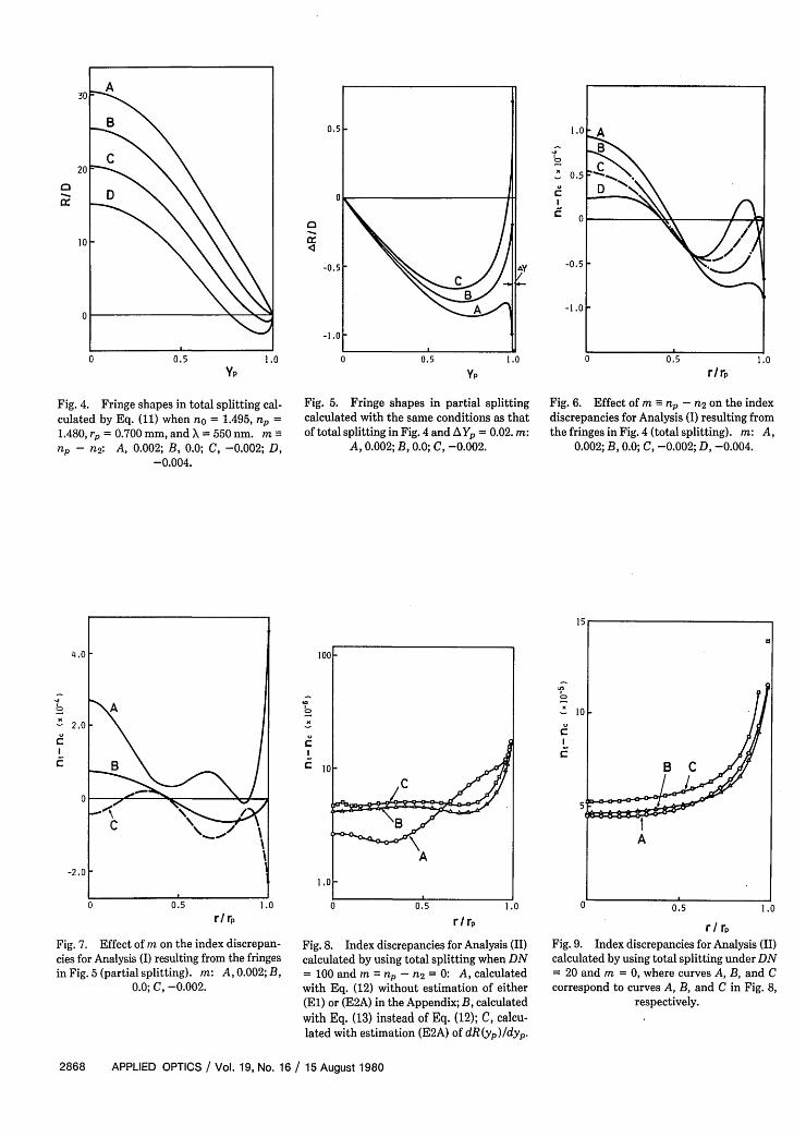
Fig. 4. Fringe shapes in total splitting cal-culated by Eq. (11) when no = 1.495, np =1.480, rp = 0.700 mm, and X = 550 nm. m -np - n2: A, 0.002; B, 0.0; C, -0.002; D,

-0.004.

4.0

2,0

0

-2.0

0 0.5 1.0

r/ rp

Fig. 7. Effect of m on the index discrepan-cies for Analysis (I) resulting from the fringesin Fig. 5 (partial splitting). m: A, 0.002; B,

0.0; C, -0.002.

0

ix

YP

Fig. 5. Fringe shapes in partial splittingcalculated with the same conditions as thatof total splitting in Fig. 4 and AYp = 0.02. m:

A, 0.002; B, 0.0; C, -0.002.

10

C~~~~

0 0.5 1.0r rp

Fig. 8. Index discrepancies for Analysis (II)calculated by using total splitting when DN= 100 and m np-n2 = 0: A, calculatedwith Eq. (12) without estimation of either(El) or (E2A) in the Appendix; B, calculatedwith Eq. (13) instead of Eq. (12); C, calcu-lated with estimation (E2A) of dR(yp)/dyp.

:055

. 0.5 .0

r/rp

Fig. 6. Effect of m np - 2 on the indexdiscrepancies for Analysis (I) resulting fromthe fringes in Fig. 4 (total splitting). m: A,

0.002; B, 0.0; C, -0.002; D, -0.004.

15

O10i

B C

5-

A

0 0.5 1.0

r /rpFig. 9. Index discrepancies for Analysis (II)calculated by using total splitting under DN= 20 and m = 0, where curves A, B, and Ccorrespond to curves A, B, and C in Fig. 8,

respectively.

2868 APPLIED OPTICS / Vol. 19, No. 16 / 15 August 1980

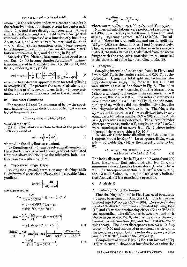
n(r) = no(l - ar2 + br4+ cr6 + dr8 ),

where no is the refractive index on a center axis, n (r) isthe refractive index at distance r from the center axis,and a, b, c, and d are distribution constants. Fringeshift R (total splitting) or shift difference AR (partialsplitting) is then expressed as a function of y includingAn, m, a, b, c, and d, where m (np - n2) and An (no- np). Solving these equations using a least squaresfit technique on a computer, we can determine distri-bution constants a, b, c, and d and no in Eq. (6).

Analysis (II)5: Here np is assumed to be equal to n2

and Eqs. (2)-(4) become simpler formulas.16 If tan4'is approximated by 4, substituting Eqs. (3) and (4) intoEq. (2) under np = n2 yields

n(u) = n2.exp .. dR(y)] dy (7)

r u/n 2 [D dy I [(n2y) 2- u2]1/2J

which is the first-order approximation for total splittingin Analysis (II). To perform the numerical calculationof the index profile, several terms in Eq. (7) were esti-mated by the procedure described in the Appendix.

IV. Computer SimulationFor reasons (1) and (2) enumerated below the speci-

men having the index distribution of Eq. (8) was se-lected for simulation:

n(u) = no - [(no - np)/(rPnP)2

]u2, (8)

where u -- r- n(r).(1) This distribution is close to that of the practical

LFR expressed as

n(r) = no1 - ! Ar2), (9)

where A is the distribution constant.(2) Equations (2)-(5) can be solved mathematically.

Here the fringe shape and fringe gradient calculatedfrom the above solution give the refractive-index dis-tribution even when np s'- n2 .

A. Theoretical Fringe ShapeSolving Eqs. (2)-(5), refraction angle 4, fringe shift

R, differential coefficient dR/dy, and observable fringegradient

are

dRdyp d(ysec)

expressed asP 2vY -n ([Am -

[A m (vY)2]- 2

+ [1 - (vY)2 ]1/

212/(Am - 1))

+ 2[sin'(Y) - sin'(vY)],

RID = P np JA 'o - 2 [1 - (Y)2]1/2

- 2 [Y tan4 + 2 (1 - y2)1/2]),

d(R/D) = rpn2 tan 21Y-tan - 3y 2 + vAMY 1AM -y2 )2/2

- Tyn'o - (1_ - y2)1/21

d(RID) rn2 iT=d Y, X si , (13)

where Am = no/(no - n), Y - y/rp, and Yp yp/rp.Numerical calculations were performed assuming no1.495, np = 1.480, rp = 0.700 mm, X = 550 nm, and

m(- np - n2 ) ranging from -0.004 to 0.002. The cal-culated fringes for total splitting and partial splitting(AYp = 0.02) are shown in Figs. 4 and 5, respectively.Then, to examine the accuracy of the respective analysismethod, the index values (nc) calculated from the abovefringes with the respective procedure were comparedto the theoretical value (nt) according to Eq. (8).

B. Analysis (I)Sampling intervals of the fringes shown in Figs. 4 and

5 were 0.05 Yp in the center region and 0.02 Yp at theperiphery. Using the total splitting technique, theindex discrepancies (nt - nc) for m = -0.004 - 0.002were within +1.0 X 10-4 as shown in Fig. 6. The indexdiscrepancies (nt - nc) resulting from the fringes in Fig.5 show a tendency to increase in the sequence: m = 0< m = -0.002 < m = 0.002. The index discrepancieswere almost within +3.0 X 10-4 (Fig. 7), and the none-quality of np with n2 did not significantly affect theresulting value of the refractive index. The fringes, fornp = n2 and the various AYp, were divided into twentyequal parts (dividing number DN = 20), and the Anal-ysis (I) procedure was performed. The curves for indexdiscrepancy vs r/rp under AYp ranging from 0.01 to 0.10were superimposed on curve B in Fig. 7 whose indexdiscrepancies were within +8 X 10-5.

In Analysis (I) the index distribution of the specimenis approximated by Eq. (6). Least squares fitting whenDN = 20 yields Eq. (14) as the closest profile to Eq.(8):

n(r) = no (1 - 2.09 X 10-2 r2 + 7.64 X 10- r4

+ 3.24 X 10-4 r6 - 3.87 X 10-4 r8

). (14)

The index discrepancies in Figs. 6 and 7 were about 200times larger than that calculated with Eq. (14), theminimum value attainable by Analysis (I) when DN =20. The discrepancies within +8 X 10-5 when np = n2

and +3 X 10-4 when I np - n2 < 0.002 clearly indicatethat Analysis (I) is a practicable procedure.

C. Analysis(ll)

1. Total Splitting TechniqueFirst the fringe of m = 0 in Fig. 4 was used because m

= 0 must be assumed in Analysis (II). The fringe wasdivided into 100 points (DN = 100). Refractive index

(10) nc at each divided point was calculated by using Eqs.(12) and (7) without estimating either (El) or (E2A) inthe Appendix. The difference between nc and nt isshown in curve A of Fig. 8, which is the sum of the errorcoming from estimation (E3) and the inevitable one of

(11) this theory. The index discrepancy was <3 X 10-6 upto r/rp = 0.50 and increased precipitously with r/rp inthe periphery region, but the index discrepancy was sosmall, <2 X 10-5, even at the periphery.

(12) Comparison of curve B [using Eq. (13) instead of Eq.(12)] with curve A shows that introduction of estimation

15 August 1980 / Vol. 19, No. 16 / APPLIED OPTICS 2869

(6)

2, AB

a~ ~C

-2.0

0 0.5 1.0r/ rp

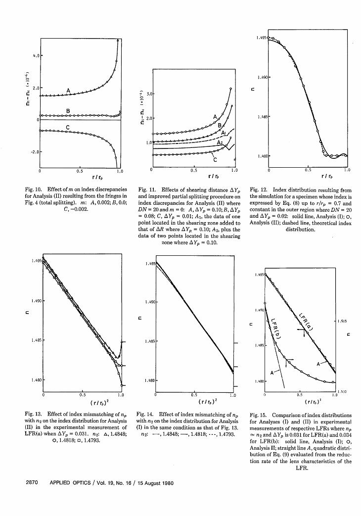
Fig. 10. Effect of m on index discrepanciesfor Analysis (II) resulting from the fringes inFig. 4 (total splitting). m: A, 0.002; B, 0.0;

C, -0.002.

I .490

C

1 .485

1.480

1.0 …A- 4

C0 0,5 1.0

r rp

Fig. 11. Effects of shearing distance Ypand improved partial splitting procedure onindex discrepancies for Analysis (II) whereDN = 20 and m = 0: A, Yp = 0.10; B, AYp= 0.08; C, Yp = 0.01; Al, the data of onepoint located in the shearing zone added tothat of AR where AYp = 0.10; A2 , plus thedata of two points located in the shearing

zone where A Yp = 0.10.

C

C

r I rp

Fig. 12. Index distribution resulting fromthe simulation for a specimen whose index isexpressed by Eq. (8) up to r/rp = 0.7 andconstant in the outer region where DN = 20and Yp = 0.02: solid line, Analysis (I); 0,Analysis (II); dashed line, theoretical index

distribution.

C

( r r) 2 ( r/ rp ) 2

Fig. 13. Effect of index mismatching of npwith n2 on the index distribution for Analysis(II) in the experimental measurement ofLFR(a) when AY = 0.031. n2 : , 1.4848;

0, 1.4818; , 1.4793.

Fig. 14. Effect of index mismatching of npwith n2 on the index distribution for Analysis(I) in the same condition as that of Fig. 13.

n2: --- , 1.4848;-, 1.4818; --- , 1.4793.

Fig. 15. Comparison of index distributionsfor Analyses (I) and (II) in experimentalmeasurements of respective LFRs where np- n2 and AYp is 0.031 for LFR(a) and 0.034

for LFR(b): solid line, Analysis (I); 0,Analysis II; straight line A, quadratic distri-bution of Eq. (9) evaluated from the reduc-tion rate of the lens characteristics of the

LFR.

2870 APPLIED OPTICS / Vol. 19, No. 16 / 15 August 1980

I .515

1.510

( r rp 2

(El) brought a slight increase in the index discrepancyin the center axis region and a slight decrease at theperiphery. As shown in curve C, adding estimation(E2A) scarcely increased the index discrepancy in theentire region.

Considering that it is difficult in practice to divide thefringe into 100 parts, the simulation under the divisioninto 20 parts (DN = 20) is shown in curves A, B, and Cof Fig. 9. While the errors were about ten times largerthan those of the corresponding curve in Fig. 8, it is in-teresting to note that the discrepancies were still within10-4 in the whole region. It should also be noted thatcurve C corresponds to the simulation of the practicalprocedure in the total splitting method.

To examine the effect of the nonequality of np withn2, the indexes were calculated by using the fringes inFig. 4, where the mode of dividing the fringe curves wasthe same as in Analysis (I). As shown in Fig. 10, indexdiscrepancies show a tendency to increase in the se-quence: m = 0 < m = -0.002 < m = 0.002, and theirerrors for m #d 0 increased remarkably at the peripherycompared with the corresponding ones in Analysis (I)(Fig. 6).

2. Partial Splitting TechniqueIndex discrepancies (nt - n) resulting from the

fringes in Fig. 5 were almost the same as those in Fig. 10.The effect of AYp values on the index discrepancy isshown in Fig. 11, where DN was 20. The errors in-creased exponentially with r/rp. At a fixed r/rp theindex discrepancy decreased with a decrease in shearingdistance A Yp and approached the corresponding valueof the total splitting method with the same DN, becausethe discrepancy for the total splitting method is thetheoretical limiting value for the partial splittingmethod. In practice the total splitting method is ap-plicable only to a fine fibrous specimen. The partial

1.495

1.490 -

1.485

0 0.5 1.0

( r rp)

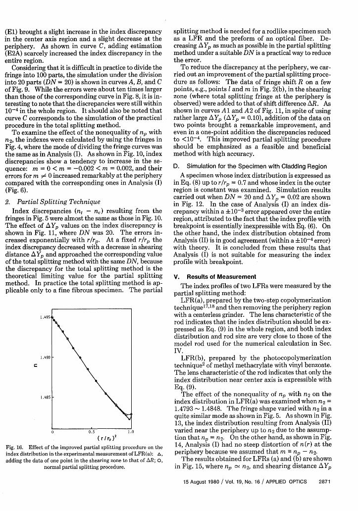
Fig. 16. Effect of the improved partial splitting procedure on theindex distribution in the experimental measurement of LFR(a): A,adding the data of one point in the shearing zone to that of AR; O,

normal partial splitting procedure.

splitting method is needed for a rodlike specimen suchas a LFR and the preform of an optical fiber. De-creasing AYp as much as possible in the partial splittingmethod under a suitable DN is a practical way to reducethe error.

To reduce the discrepancy at the periphery, we car-ried out an improvement of the partial splitting proce-dure as follows: The data of fringe shift R on a fewpoints, e.g., points and m in Fig. 2(b), in the shearingzone (where total splitting fringe at the periphery isobserved) were added to that of shift difference AR. Asshown in curves Al and A2 of Fig. 11, in spite of usingrather large AYp (AYp = 0.10), addition of the data ontwo points brought a remarkable improvement, andeven in a one-point addition the discrepancies reducedto <10-4. This improved partial splitting procedureshould be emphasized as a feasible and beneficialmethod with high accuracy.

D. Simulation for the Specimen with Cladding Region

A specimen whose index distribution is expressed asin Eq. (8) up to r/rp = 0.7 and whose index in the outerregion is constant was examined. Simulation resultscarried out when DN = 20 and A Yp = 0.02 are shownin Fig. 12. In the case of Analysis (I) an index dis-crepancy within a +10-3 error appeared over the entireregion, attributed to the fact that the index profile withbreakpoint is essentially inexpressible with Eq. (6). Onthe other hand, the index distribution obtained fromAnalysis (II) is in good agreement (within a +10-4 error)with theory. It is concluded from these results thatAnalysis (I) is not suitable for measuring the indexprofile with breakpoint.

V. Results of MeasurementThe index profiles of two LFRs were measured by the

partial splitting method:LFR(a), prepared by the two-step copolymerization

technique' 7"18 and then removing the periphery regionwith a centerless grinder. The lens characteristic of therod indicates that the index distribution should be ex-pressed as Eq. (9) in the whole region, and both indexdistribution and rod size are very close to those of themodel rod used for the numerical calculation in Sec.IV.

LFR(b), prepared by the photocopolymerizationtechnique2 of methyl methacrylate with vinyl benzoate.The lens characteristic of the rod indicates that only theindex distribution near center axis is expressible withEq. (9).

The effect of the nonequality of np with n2 on theindex distribution in LFR(a) was examined when n2 =

1.4793 - 1.4848. The fringe shape varied with n2 in aquite similar mode as shown in Fig. 5. As shown in Fig.13, the index distribution resulting from Analysis (II)varied near the periphery up to n2 due to the assump-tion that np = n2. On the other hand, as shown in Fig.14, Analysis (I) had no steep distortion of n(r) at theperiphery because we assumed that m n - n2.

The results obtained for LFRs (a) and (b) are shownin Fig. 15, where np n2, and shearing distance AYp

15 August 1980 / Vol. 19, No. 16 / APPLIED OPTICS 2871

is 0.031 for LFR(a) and 0.034 for LFR(b), respectively.In either specimen the respective profile from Analysis(I) is in good agreement with that from Analysis (II) overthe entire range. Straight line A shows the quadraticdistribution of Eq. (9) whose slope was evaluated fromthe reduction rate of the lens characteristics of the LFR.The point at which the distribution curve of LFR(b)deviates from line A is consistent with the radius inwhich the index distribution is expressible with Eq.(9).

As shown in Fig. 16, in spite of np 5=1 n2, the improvedpartial splitting procedure (using the data of one pointlocated in the shearing zone) improved the index dis-tribution in the periphery region. Now the improvedpartial splitting procedure is also assumed to be a morepracticable method with higher accuracy.

VI. ConclusionComputer simulation indicates the following im-

portant aspects:(1) Analysis (II), the partial splitting method is more

practicable than total splitting for the rodlike specimen.Using both shearing distance A Yp as small as possibleand suitable DN in the former yields a high accuracy.In addition, the improved partial splitting procedure(adding some data of points located in the shearingzone) facilitates reduction of error especially in theperiphery region.

(2) If the index profile of the specimen is closely ex-pressed with Eq. (6), Analysis (I) gives the same orderof accuracy as Analysis (II) and, in particular, higheraccuracy than Analysis (II) when np n2. For theindex profile with breakpoint, Analysis (I) is inferior toAnalysis (II).

The index profiles of the two selected LFRs werecalculated by the above analysis procedures. For theirrespective LFR, both procedures yield superimposableprofiles consistent with that of the lens characteristicof the specimen. It is also shown that the nonequalityof n2 with np has a deleterious effect for Analysis (II)but is negligible for Analysis (I). All these results metthe expectations anticipated from the simulation.

The improved partial splitting procedure is believedto be a practicable method of high accuracy for deter-mining the index profile of a rodlike specimen.

Appendix: Estimation of the Terms in Eq. (7)

(El) dR(y)/dy

The gradient of the fringe is not dR(y)/dy butdR(yp)/dyP, where yp = y-sec'. As expressed in termsof a Taylor series expansion:

tan = + 1,3

+ 2 Q5 +3 15

secV = + 1 2+ 4+2 24

Strictly speaking, the assumption that tan4 = t' doesnot lead logically to sec4 = 1. But dR (y)/dy is assumedto be equal to dR(yp)/dyp, because ' is very small inpractice.

(E2) dR(yp)/dypE2A (total splitting method): Using Lagrange's

interpolation, the fringe containing five consecutivepoints is expressed by a fourth-order polynomialequation from which the fringe gradient in this rangeis calculated.

E2B (partial splitting method): The fringe gradientat yp is estimated by Eq. (Al) according to Eq. (1):

dR(yp) AR(yP)

dyp AyP(Al)

where yp = yp. It should be noted that the error in-creases with an increase in Ayp.

(E3) Estimation of the Integral Part in Eq. (7)Since the denominator of the integrand becomes zero

at y = u/n2 , the following procedure is carried out,which is different from that of Iga et al. 5 When thefringe gradients at Yp,k and Yp,k+1 are Ak and Ak+1, re-spectively, fringe gradient Ap at yp located between Yp,kand Yp,k+l can be expressed as

A, = I-yp + m, (A2)

where I = (Ak+1 - Ak)/(Yp,k+1 - Yp,k), andm = (AkYp,k+1 - Ak+1Yp,k)/(Yp,k+1 - Yp,k),

and the following equation results:

frp dR(y) dyJu/n 2 dy [(n2y)

2- u2 ]/ 2

1 n-i[I(y

2- y2,,)1/

2+ m ln [y + (y2

_ y2

)l/2]Yp,j+1, (A3)

fl2 j=0 y,+

where Yp,i = i/n 2 , and Yp,n+1 = rp. It is also possibleto use higher polynomial equations instead of Eq. (A2)to solve mathematically the integral part of Eq. (7).Bearing in mind that breakpoints occasionally appearin the observed fringe, this estimation procedure is moreconvenient for this situation.

References1. Y. Ohtsuka and Y. Hatanaka, Appl. Phys. Lett. 29, 735 (1976).2. Y. Ohtsuka and I. Nakamoto, Appl. Phys. Lett. 29, 559 (1976).3. Y. Ohtsuka and Y. Shimizu, Appl. Opt. 16, 1050 (1977).4. Registered trade name of Carl Zeiss, Jena, East Germany.5. Y. Kokubun and K. Iga,'Trans. IECE Jpn. E60, 702 (1977).6. M. Ikeda, M. Tateda, and H. Yoshikiyo, Appl. Opt. 14, 814

(1975).7. J. A. Arnaud and R. M. Derosier, Bell Syst. Tech. J. 55, 1489

(1976).

8. H. M. Presby and I. P. Kaminow, Appl. Opt. 15, 3029 (1976).9. T. Okoshi and K. Hotate, Appl. Opt. 15, 2756 (1976).

10. P. L. Chu, Electron. Lett. 13, 736 (1977).11. E. Brinkmeyer, Appl. Opt. 16, 2802 (1977).

12. D. Marcuse, Appl. Opt. 18, 9 (1979).13. P. L. Chu and T. Whitbread, Appl. Opt. 18, 1117 (1979).

14. L. S. Watkins, Appl. Opt. 18, 2214 (1979).15. G. D. Kahl and D. C. Mylin, J. Opt. Soc. Am. 55, 364 (1965).16. A. M. Hunter II and P. W. Schreiber, Appl. Opt. 14, 634

(1975).

17. Y. Ohtsuka, T. Senga, and H. Yasuda, Appl. Phys. Lett. 25, 659(1974).

18. Y. Ohtsuka, T. Sugano, and Y. Koike, Am. Chem. Soc. Div. Org.Coat. Plast. Chem. Pap. 40, 382 (1979).

2872 APPLIED OPTICS / Vol. 19, No. 15 / 1 August 1980