Determination of the Reachable Workspace of 6-3 Stewart Platform Mechanism · Abstract—In this paper, a novel geometrical methodology is introduced for determining the reachable

Abstract—In this paper, a novel geometrical methodology is

introduced for determining the reachable workspace of 6-3

Stewart Platform Mechanism. The reachable workspace is one

of the significant characteristic in determining the feasibility of

utilizing SPM as a machine tool structure. The proposed

method based on a geometrical approach is rather

straightforward to evaluate the reachable workspace.

Basically, it is based on determining attainable locations of

three vertices for all possible leg configurations as all

constraints dealing with legs and joints are taken into

consideration.

Index Terms—Kinematics, machine tool, workspace, Stewart

Platform Mechanism.

I. INTRODUCTION

Stewart Platform Mechanism (SPM) has been extensively

utilized in many practical engineering applications ranging

from CNC machining to satellite dish positioning since

D.Stewart proposed SPM as a flight simulator [1]. Although

it has recently received considerable attention from many

researchers because of its advantages such as high structural

rigidity, accuracy, force/torque capacity, there are major

drawbacks such as complex forward kinematics and limited

workspace. Therefore, researchers have focused on

workspace of SPM and introduced many valuable studies for

last three decades.

Merlet classified workspace determination methods into

three groups, namely discretization methods, geometrical

methods, and numerical methods [2]. Gossellin proposed the

geometrical method for determining the constant orientation

workspace of 6 degree of freedom parallel manipulator. [3].

Since SPM has also been utilized in CNC machining / 5-axis

machining operations, some researchers have carried out

some studies to achieve the knowledge of shape and size of

workspaces and boundaries of SPMs [4]- [11].

Reachable workspace is a set which contains all the

positions that can be achieved by a reference point on the

end-effector [12] The knowledge of size and shape of

Serdar AY is with the Aeronautical and Astronautical Engineering

Department, Turkish Air Force Academy, Yeşilyurt-İstanbul, Turkey

(e-mail: say@ hho.edu.tr).

O.Erguven VATANDAŞ is with the Turkish Air Force Academy,

Yeşilyurt-İstanbul, Turkey (e-mail: [email protected]).

Abdurrahman HACIOĞLU is with the Aeronautical and Astronautical

Engineering Department, Turkish Air Force Academy, Yeşilyurt-İstanbul,

Turkey ( e-mail: hacioglu@ hho.edu.tr).

workspace and boundary of SPM is of a great importance to

locate the workpiece properly in order to avoid collisions

between the cutting tool and the workpiece. Therefore, the

reachable workspace is one of the significant characteristic in

determining the feasibility of utilizing SPM as a machine tool

structure.

The proposed method based on a geometrical approach is

rather straightforward to evaluate the reachable workspace.

Basically, it is based on determining attainable locations of

three vertices for all possible leg configurations as all

constraints dealing with legs and joints are taken into

consideration.

The organization of this study is as follows. First, in

Section II, the description of 6-3 SPM is presented.

Secondly, in Section III, the proposed geometrical algorithm

is introduced in detail. Thirdly, in Section IV, the

implementation of the proposed method is presented.

Finally, conclusions are made in Section V.

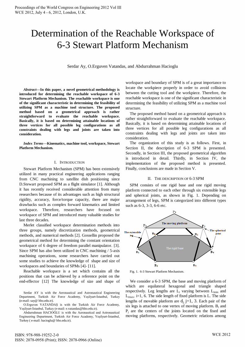
II. THE DESCRIPTION OF 6-3 SPM

SPM consists of one rigid base and one rigid moving

platform connected to each other through six extensible legs

and spherical joints, as shown in Fig. 1. Depending on

arrangement of legs, SPM is categorized into different types

such as 6-3, 3-3, 6-6 etc.

Fig. 1. 6-3 Stewart Platform Mechanism.

We consider a 6-3 SPM, the base and moving platform of

which are equilateral hexagonal and triangle shaped

respectively. Leg lengths are Li varying between Limin and

Limax, i=1, 6. The side length of fixed platform is L. The side

lengths of movable platform are dj, j=1, 3. Each pair of the

six legs is attached to one vertex of moving platform. Bi and

Pj are the centers of the joints located on the fixed and

moving platforms, respectively. Geometric relations among

Determination of the Reachable Workspace of

6-3 Stewart Platform Mechanism

Serdar Ay, O.Erguven Vatandas, and Abdurrahman Hacioglu

Proceedings of the World Congress on Engineering 2012 Vol III WCE 2012, July 4 - 6, 2012, London, U.K.

ISBN: 978-988-19252-2-0 ISSN: 2078-0958 (Print); ISSN: 2078-0966 (Online)

WCE 2012

vertices P1, P2, P3 and other parameters were presented by

Nanua et al. [13].

III. THE PROPOSED METHODOLOGY

The methodology consists of three steps. In each step, the

position of one of the vertices is determined. The details of

steps are presented in the following sections:

A. The Determination of Position of Vertex P1

The coordinates (p1x, p1y, p1z) of vertex P1 in Fig. 3 are

determined by varying lengths of L1, L2 and Ф1 with respect

to the constraints of L1, L2, and joints.

Lbi and rj are the distances between Bi and Oj, and

between Pj and Oj, respectively, as shown in Fig. 2.

Fig. 2. The location of vertex P1.

It is necessary to express Lb1, Lb2 and r1 for vertex P1 in

terms of leg lengths. These expressions include the

following: 2 2 2

1 21 (1)

2b

L L LL

L

2 1 (2)b bL L L

2 21 1 1 (3)br L L

The coordinates (x01, y01) of O1 are given by the following

equations:

01 1 11 cos( ) (4)b bx x L

01 1 11sin ( ) (5)b b

y y L

where (xb1, yb1) are the coordinates of B1 and α1 is the angle

between x axis and O1, as shown in Fig. 3.

The coordinates (p1x, p1y, p1z) of vertex P1 are given by the

following equations:

1 1 1 1 1)cos sin( (6)

x Op x r

1 1 1 1 1)cos cos( (7)y Op y r

1 1 1sin (8)zp r

where Ф1 determined by considering the limitations of joints

is the angle between the planes of x-y and the triangle

B1P1B2.

Varying L1, L2 and Ф1 discretely with respect to the

related constraints describes the entire achievable positions

of the first vertex.

Fig. 3. Top view of the fixed base.

B. The Determination of Position of Vertex P2

In this phase, the lengths of L3 and L4 are varied discretely

with respect to the related constraints. The coordinates (p2x,

p2y, p2z) of vertex P2 are determined by considering L3, L4,

and the coordinates (p1x, p1y, p1z) of vertex P1 determined in

previous phase.

In order to determine P2 (p2x, p2y, p2z) the geometrical

relation between P1 and P2 is taken into account. Vertex P2

may be located on the sphere centered at P1 with radius d1,

as shown in Fig 4.

Fig. 4. The sphere centered at P1 with d1 radius.

Let t be the axis on x-y plane which is perpendicular to the

line B3B4a and passes through O2 as shown in Fig. 5. Varying

lengths of L3 and L4 and keeping P1 fixed, vertex P2 moves in

the circle centered at O2 with radius r2, which lies on t-z

plane. In order to determine the coordinates (p2x, p2y, p2z)

of vertex P2, it is necessary to figure out whether or not the

sphere centered at P1 and the circle centered at O2 intersect.



WCE 2012

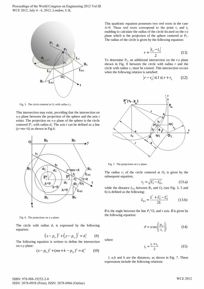
Fig. 5. The circle centered at O2 with radius r2.

This intersection may exist, providing that the intersection on

x-y plane between the projection of the sphere and the axis t

exists. The projection on x-y plane of the sphere is the circle

centered Pı1 with radius d1. The axis t can be defined as a line

(y=mx+k) as shown in Fig.6.

Fig. 6. The projections on x-y plane.

The circle with radius d1 is expressed by the following

equation:

22 2

1 1 1(9)

x yx p y p d

The following equation is written to define the intersection

on x-y plane:

1

2 2 21 1( ) ( ) (10)x yx p mx k p d

This quadratic equation possesses two reel roots in the case

Δ>0. These reel roots correspond to the point t1 and t2

enabling to calculate the radius of the circle located on the t-z

plane which is the projection of the sphere centered at P1.

The radius of the circle is given by the following equation:

2 1(11)

2

t tr

To determine P2, an additional intersection on the t-z plane

shown in Fig. 8 between the circle with radius r and the

circle with radius r2 must be existed. This intersection occurs

when the following relation is satisfied:

2 2 (12)r r l r r

Fig. 7. The projections on t-z plane.

The radius r2 of the circle centered at O2 is given by the

subsequent equation;

2 22 3 3 (13.a)br L L

while the distance Lb3 between B3 and O2 (see Fig. 3, 5 and

6) is defined as the following: 2 2 2

3 43 (13.b)

2b

L L LL

L

θ is the angle between the line P1ııO2 and t axis. θ is given by

the following equation:

1

0

tan (14)zpa

t

where

1 2

02

(15)t t

t

l, a,b and h are the distances, as shown in Fig. 7. These

expressions include the following relations:



WCE 2012

2 2

0 1 (16)zt Pl

2 2 2

2

2(17)

r l ra

l

(18)b l a

2 2 (19)h r a

The projection on t-z plane of vertex P2 (p2x, p2y, p2z) is

2 2 2( , )ıı ıı ııP tp zp and 2

ııtp , 2

ıızp are given by the following

equations:

2 cos( ) (20)ııtp b

2 sin( ) (21)ıızp b

The coordinates of points A and B on t-z plane are

2 .sin( ) (22)ıı

At tp h

2 .cos( ) (23)ıı

Az tp h

2 .sin( ) (24)ıı

Bt tp h

2 .cos( ) (25)ıı

Bz tp h

The coordinates (x03, y03) of O2 are given by the following

equations:

02 23 3 cos( ) (26)b bx x L

02 3 23sin( ) (27)b b

y y L

where (xb3, yb3) are the coordinates of B3. The projections on

x-y plane of points A and B can be written as

2 2sin( ) (28)A O Ax x t

2 2cos( ) (29)A O Ay y t

2 2sin( ) (30)B BOx x t

2 2cos( ) (31)B BOy y t

xA , xB and yA , yB are the solutions of the coordinates (p2x)

and (p2y), respectively while zA and ,zB are the solutions of

p2z. Each solution of (p2x, p2y, p2z) is accepted for the vertex

P2, if the associated constraints are satisfied.

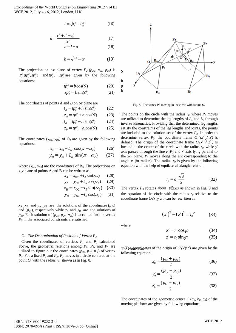
C. The Determination of Position of Vertex P3

Given the coordinates of vertices P1 and P2 calculated

above, the geometric relations among P1, P2, and P3 are

utilized to figure out the coordinates (p3x, p3y, p3z) of vertex

P3. For a fixed P1 and P2, P3 moves in a circle centered at the

point Oı with the radius r0, shown as in Fig. 8.

Sizing of Graphics

Most charts graphs and tables are one column wide (3 1/2

inches or 21 picas) or two-column width (7 1/16 inches, 43

picas wide). We recommend that you avoid sizing figures

less than one column wide, as extreme enlargements may

Fig. 8. The vertex P3 moving in the circle with radius r0.

The points on the circle with the radius r0, where P3 moves

are utilized to determine the leg lengths of L5 and L6 through

inverse kinematics. Providing that the determined leg lengths

satisfy the constraints of the leg lengths and joints, the points

are included to the solution set of the vertex P3. In order to

determine vertex P3, the coordinate frame O ı(x

ı y

ı z

ı) is

defined. The origin of the coordinate frame Oı(x

ı y

ı z

ı ) is

located at the center of the circle with the radius r0. while yı

axis passes through the line P1P2 and x

ı axis lying parallel to

the x-y plane. P3 moves along the arc corresponding to the

angle φ (in radian). The radius r0 is given by the following

equation with the help of equilateral triangle relation:

0 1

3(32)

2r d

The vertex P3 rotates about yaxis as shown in Fig. 9 and

the equation of the circle with the radius r0 relative to the

coordinate frame Oı(x

ıy

ı z

ı ) can be rewritten as

2 2 2

0 (33)x z r

where

0 cos (34)x r

0 sin (35)z r

The coordinates of

The coordinates of the origin of OI(x

ıy

ız

ı) are given by the

following equation:

1 20

( )(36)

2

x xp px

1 2

0

( )(37)

2

y yp py

1 20

( )(38)

2

z zp pz

The coordinates of the geometric center C (a0, b0, c0) of the

moving platform are given by following equations:



WCE 2012

The coordinates of the geometric center C (a0, b0, c0) of the

moving platform are given by following equations:

0 30

2(39)

3

xx px

0 3

0

2(40)

3

yy py

0 30

2(41)

3

zz pz

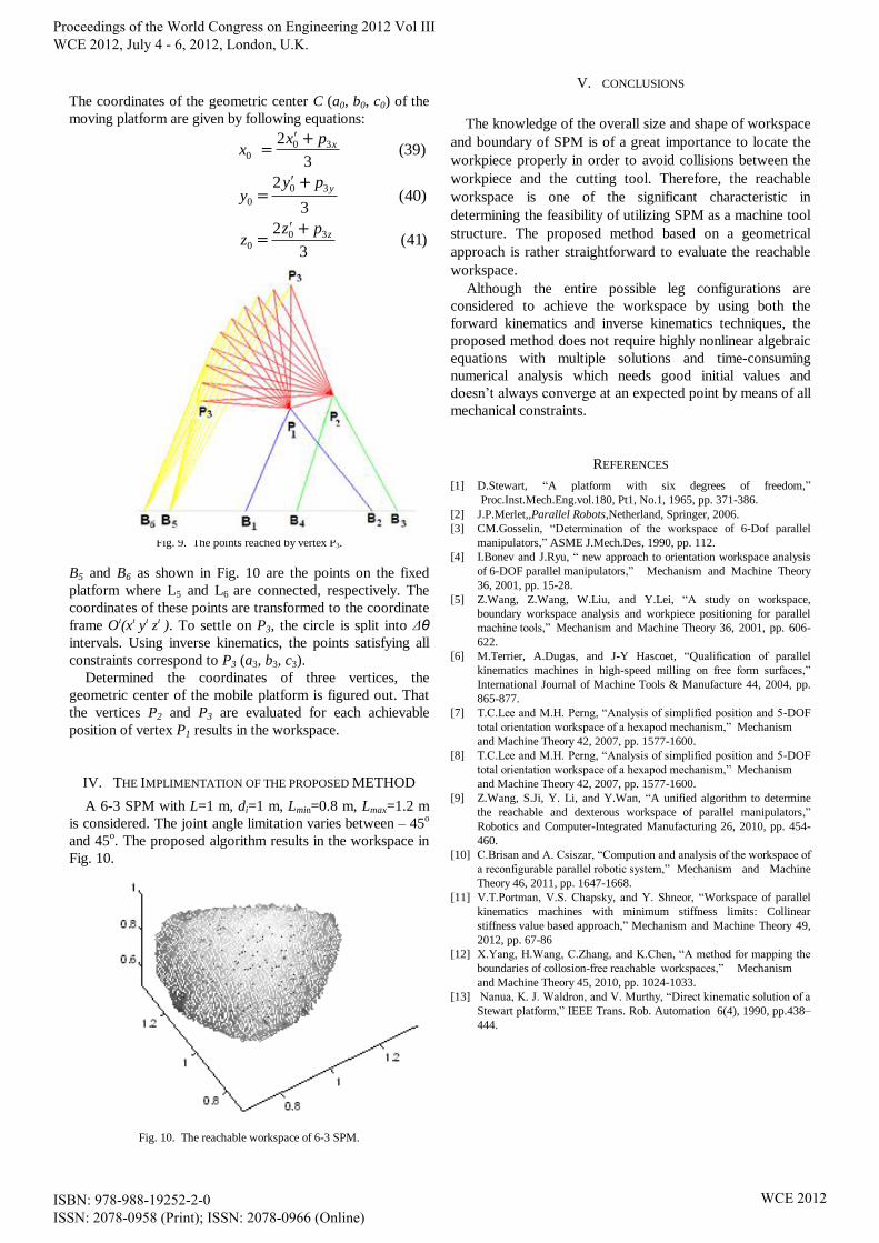
Fig. 9. The points reached by vertex P3.

B5 and B6 as shown in Fig. 10 are the points on the fixed

platform where L5 and L6 are connected, respectively. The

coordinates of these points are transformed to the coordinate

frame Oı(x

ı y

ı z

ı ). To settle on P3, the circle is split into Δθ

intervals. Using inverse kinematics, the points satisfying all

constraints correspond to P3 (a3, b3, c3).

Determined the coordinates of three vertices, the

geometric center of the mobile platform is figured out. That

the vertices P2 and P3 are evaluated for each achievable

position of vertex P1 results in the workspace.

IV. THE IMPLIMENTATION OF THE PROPOSED METHOD

A 6-3 SPM with L=1 m, di=1 m, Lmin=0.8 m, Lmax=1.2 m

is considered. The joint angle limitation varies between – 45o

and 45o. The proposed algorithm results in the workspace in

Fig. 10.

0.8

1

1.2

0.8

1

1.2

0.6

0.8

1

Fig. 10. The reachable workspace of 6-3 SPM.

V. CONCLUSIONS

The knowledge of the overall size and shape of workspace

and boundary of SPM is of a great importance to locate the

workpiece properly in order to avoid collisions between the

workpiece and the cutting tool. Therefore, the reachable

workspace is one of the significant characteristic in

determining the feasibility of utilizing SPM as a machine tool

structure. The proposed method based on a geometrical

approach is rather straightforward to evaluate the reachable

workspace.

Although the entire possible leg configurations are

considered to achieve the workspace by using both the

forward kinematics and inverse kinematics techniques, the

proposed method does not require highly nonlinear algebraic

equations with multiple solutions and time-consuming

numerical analysis which needs good initial values and

doesn’t always converge at an expected point by means of all

mechanical constraints.

REFERENCES

[1] D.Stewart, “A platform with six degrees of freedom,”

Proc.Inst.Mech.Eng.vol.180, Pt1, No.1, 1965, pp. 371-386.

[2] J.P.Merlet,,Parallel Robots,Netherland, Springer, 2006.

[3] CM.Gosselin, “Determination of the workspace of 6-Dof parallel

manipulators,” ASME J.Mech.Des, 1990, pp. 112.

[4] I.Bonev and J.Ryu, “ new approach to orientation workspace analysis

of 6-DOF parallel manipulators,” Mechanism and Machine Theory

36, 2001, pp. 15-28.

[5] Z.Wang, Z.Wang, W.Liu, and Y.Lei, “A study on workspace,

boundary workspace analysis and workpiece positioning for parallel

machine tools,” Mechanism and Machine Theory 36, 2001, pp. 606-

622.

[6] M.Terrier, A.Dugas, and J-Y Hascoet, “Qualification of parallel

kinematics machines in high-speed milling on free form surfaces,”

International Journal of Machine Tools & Manufacture 44, 2004, pp.

865-877.

[7] T.C.Lee and M.H. Perng, “Analysis of simplified position and 5-DOF

total orientation workspace of a hexapod mechanism,” Mechanism

and Machine Theory 42, 2007, pp. 1577-1600.

[8] T.C.Lee and M.H. Perng, “Analysis of simplified position and 5-DOF

total orientation workspace of a hexapod mechanism,” Mechanism


[9] Z.Wang, S.Ji, Y. Li, and Y.Wan, “A unified algorithm to determine

the reachable and dexterous workspace of parallel manipulators,”

Robotics and Computer-Integrated Manufacturing 26, 2010, pp. 454-

460.

[10] C.Brisan and A. Csiszar, “Compution and analysis of the workspace of

a reconfigurable parallel robotic system,” Mechanism and Machine

Theory 46, 2011, pp. 1647-1668.

[11] V.T.Portman, V.S. Chapsky, and Y. Shneor, “Workspace of parallel

kinematics machines with minimum stiffness limits: Collinear

stiffness value based approach,” Mechanism and Machine Theory 49,

2012, pp. 67-86

[12] X.Yang, H.Wang, C.Zhang, and K.Chen, “A method for mapping the

boundaries of collosion-free reachable workspaces,” Mechanism


[13] Nanua, K. J. Waldron, and V. Murthy, “Direct kinematic solution of a

Stewart platform,” IEEE Trans. Rob. Automation 6(4), 1990, pp.438–

444.



WCE 2012

Documents

Determination of the Reachable Workspace of 6-3 Stewart Platform Mechanism · Abstract—In this paper, a novel geometrical methodology is introduced for determining the reachable