Embed Size (px)
Citation preview

DETERMINATION OF THE EFFECTS OF FISH SIZE AND FEED PELLET SIZE
ON THE SETTLING CHARACTERISTICS OF RAINBOW TROUT ( SALMO
GAIRDNERI ) CULTURE CLEANING WASTES
by
DOUGLAS EDWARD THOMSON
B.Sc. (The University of British Columbia, 1983)
A THESIS SUBMITTED IN PARTIAL FULFILMENT OF
THE REQUIREMENTS FOR THE DEGREE OF
MASTER OF SCIENCE
in
THE FACULTY OF GRADUATE STUDIES
DEPARTMENT OF BIO-RESOURCE ENGINEERING
We accept this thesis as conforming
to the required standard
THE UNIVERSITY OF BRITISH COLUMBIA
November, 1986
® DOUGLAS EDWARD THOMSON, 1986

In presenting this thesis in partial fulfilment of the requirements for an advanced
degree at the University of British Columbia, I agree that the Library shall make it
freely available for reference and study. I further agree that permission for extensive
copying of this thesis for scholarly purposes may be granted by the head of my
department or by his or her representatives. It is understood that copying or
publication of this thesis for financial gain shall not be allowed without my written
permission.
Department of BIO - RESOURCE ENGINEERING
The University of British Columbia 1956 Main Mall Vancouver, Canada V6T 1Y3
Date APRIL 30,1987
DE-6(3/81)

A B S T R A C T
This research reports on the determination of the effects of fish size and feed pellet
size on the settling characteristics of Rainbow trout (Salmo gairdneri) culture, tank
cleaning wastes.
Flocculant particle settling curves (Type II) were developed from settling column
analysis of cleaning wastes from 11-311 gram Rainbow trout fed a moist pellet diet
(Oregon Moist Pellet ®). Four feed pellet sizes were investigated: 3/32, 1/8, 5/32 and
3/16 inch.
Overall non-filterable residue removal curves and individual particle settling velocity
distribution curves, derived from the Type II settling curve of each fish size and feed
pellet size group, were compared. Slopes and y-intercepts of the linearized overall
non-filterable residue removal curves and individual particle settling velocity distribution
curves were compared using the Equality of Slope Test (S:SLTEST).
Results of the test for a common regression equation indicated there were no
significant differences in the proportional distribution of particle sizes within the
cleaning wastes. Variations observed in the initial rates of removal within the overall
non-filterable residue removal curves were considered insignificant
Settling trials were pooled in order to obtain single curves, characterizing the overall
solids removal rate and the individual particle settling velocity distribution of the waste
solids.
ii

TABLE OF CONTENTS
LIST OF FIGURES iv
LIST OF TABLES vi
ABSTRACT ii
ACKNOWLEDGEMENT vii
1. INTRODUCTION 1
2. LITERATURE REVIEW 7
3. THEORY 19
4. MATERIALS AND METHODS 34 4.1. Species 34 4.2. Fish Size 34 4.3. Feed Type and Pellet Size 36 4.4. Laboratory Set Up 36
4.4.1. Containment 36 4.4.2. Water Supply 36 4.4.3. Aeration 38 4.4.4. Stocking Density , 38
4.5. Settling Column 38 4.6. Experimental Procedure 40
5. RESULTS AND DISCUSSION 43
6. CONCLUSION 92
7. RECOMMENDATIONS FOR FUTURE WORK 93 7.1. Residence Time 93
7.2. Feed Type 94
REFERENCES 95
APPENDIX I 101
APPENDIX II 103
iii

LIST OF FIGURES
Figure 1.1: Removal of NH 3-N, N03, P04, and BOD as a function of solids removal (Muir, 1982) 5
Figure 2.1: Settling velocities for intact Rainbow trout excreta as a function of fish size (Warrer-Hansen, 1982) 13
Figure 2.2: Relationship between residence time and solids removal (Warrer-Hansen, 1982) 15
Figure 3.1: Schematic of an ideal rectangular sedimentation basin, indicating the settling path of discrete particles 20
Figure 3.2: Discrete particle velocity cumulative frequency distribution 23 Figure 3.3: Path trajectory of particles in discrete particle settling 24 Figure 3.4: Path trajectory of particles in flocculant particle or Type II settling 24 Figure 3.5: Type II or flocculant particle settling curves 27 Figure 3.6: Overall non-filterable residue removal curve 29 Figure 3.7: Graphical representation of the percentage of non-filterable residue
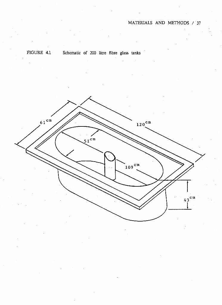
particulates with settling velocities greater than X 32 Figure 3.8: Individual particle settling velocity distribution curve 33 Figure 4.1: Schematic of 200 litre oval fibre glass tanks 37 Figure 4.2: Schematic of settling column used 39 Figure 5.1: Non-filterable residue removal for example data given in Table IV,
as a function of residence time and column depth 51 Figure 5.2: Type II or flocculant particle settling curves for example data given
in Table IV 52 Figure 5.3: Overall non-filterable residue removal curve for data given in Table IV 53 Figure 5.4: Individual particle settling velocity distribution curve for example data
in Table IV 54 Figure 5.5: Overall non-filterable residue removal curves for 11 gram Rainbow
trout fed 3/32 OMP feed pellets 55 Figure 5.6: Overall non-filterable residue removal curves for 17 gram Rainbow
trout fed 3/32 OMP feed pellets 56 Figure 5.7: Overall non-filterable residue removal curves for 21 gram Rainbow
trout fed 3/32 OMP feed pellets 57 Figure 5.8: Overall non-filterable residue removal curves for 21 gram Rainbow
trout fed 1/8 OMP feed pellets 58 Figure 5.9: Overall non-filterable residue removal curves for 41 gram Rainbow
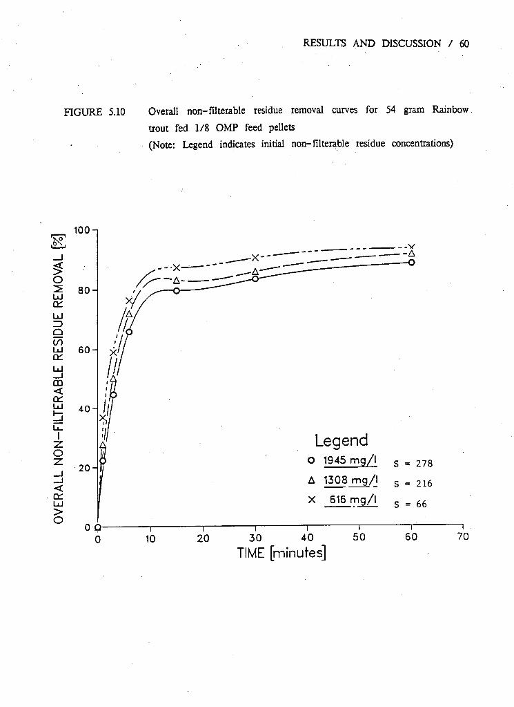
trout fed 1/8 OMP feed pellets 59 Figure 5.10: Overall non-filterable residue removal curves for 54 gram Rainbow
trout fed 1/8 OMP feed pellets 60 Figure 5.11: Overall non-filterable residue removal curves for 54 gram Rainbow
trout fed 5/32 OMP feed pellets 61 Figure 5.12: Overall non-filterable residue removal curves for 73 gram Rainbow
trout fed 5/32 OMP feed pellets 62 Figure 5.13: Overall non-filterable residue removal curves for 93 gram Rainbow
trout fed 5/32 OMP feed pellets 63 Figure 5.14: Overall non-filterable residue removal curves for 89 gram Rainbow
trout fed 3/16 OMP feed pellets 64 Figure 5.15: Overall non-filterable residue removal curves for 311 gram Rainbow
trout fed 3/16 OMP feed pellets 65
iv

Figure 5.16: Individual particle settling velocity distribution curves for 11 gram Rainbow trout fed 3/32 OMP feed pellets 66
Figure 5.17: Individual particle settling velocity distribution curves for 17 gram Rainbow trout fed 3/32 OMP feed pellets 67
Figure 5.18: Individual particle settling velocity distribution curves for 21 gram Rainbow trout fed 3/32 OMP feed pellets 68
Figure 5.19: Individual particle settling velocity distribution curvess for 21 gram Rainbow trout fed 1/8 OMP feed pellets 69
Figure 5.20: Individual particle settling velocity distribution curves for 41 gram Rainbow trout fed 1/8 OMP feed pellets 70
Figure 5.21: Individual particle settling velocity distribution curves for 54 gram Rainbow trout fed 1/8 OMP feed pellets 71
Figure 5.22: Individual particle settling velocity distribution curves for 54 gram Rainbow trout fed 5/32 OMP feed pellets 72
Figure 5.23: Individual particle settling velocity distribution curves for 73 gram Rainbow trout fed 5/32 OMP feed pellets 73
Figure 5.24: Individual particle settling velocity distribution curves for 93 gram Rainbow trout fed 5/32 OMP feed pellets 74
Figure 5.25: Individual particle settling velocity distribution curves for 89 gram Rainbow trout fed 3/16 OMP feed pellets 75
Figure 5.26: Individual particle settling velocity distribution curves for 311 gram Rainbow trout fed 3/16 OMP feed pellets 76
Figure 5.27: Variability of the y-intercept of the linearized overall non-filterable residue removal curves as a function of the initial non-filterable residue concentration 83
Figure 5.28: Overall non-filterable residue removal curve for Rainbow trout fed an OMP diet 87
Figure 5.29: Individual particle settling velocity distribution curve for Rainbow trout fed an OMP diet 88
Figure 530: Summary of capital, operating, and maintenance costs for a sedimentation basin as a function of surface area (Underwood McLellan, 1979)
89
v

LIST OF TABLES
Table I: Summary of integration calculations of flocculant particle settling curve for residence time T2 28
Table II: Weight classes and corresponding feed pellet sizes used in waste trials 35 Table III: Variability of initial non-filterable residue concentrations as a function
of column depth 47 Table IV: Non-filterable residue concentrations for a sample settling trial 49 Table V: SLTEST generated common regression equations for Figures 5.5 - 5.15 ....101
v i
ACKNOWLEDGEMENT
I would like to express my sincere thanks to the following individuals for their
contributions in making this thesis possible.
Dr. N.R. Bulley for his supervision and guidance of my M.Sc. program and, for the
valuable encouragment and patience shown throughout the production of this thesis.
I would also like to thank Prof. B. March for serving as a committee member and
for making available the South Campus Fish Nutrition Lab for the waste trials. I
would like to thank Bill McLean (Department of Fisheries and Oceans) for serving as
a committee member and for supplying the feed used in the study.
Special thanks to Hugh Sparrow and Dale Larson of the Fraser Valley Trout Hatchery
(Provincial Fish and Wildlife Branch) for supplying the Queens fish used in our trials.
A very special thanks are due to Jannice Wormsworth for her daily assistance in
feeding and caring of the fish..
Finally I would like to' thank my family and friends for their patience, encouragement
and unfailing support throughout this project
vii

1. INTRODUCTION
The effluent discharged from a freshwater trout farm or hatchery offers unique
problems in the areas of wastewater treatment and management While at times
resembling that of a domestic water supply, effluents can reach strengths more
frequently associated with conditions in a secondary sewage treatment plant
In the past when fish farms were small and few in number, discharged farm effluents
posed no significant problems. In some cases, the contribution of solids and dissolved
nutrients to oligotrophy receiving waters provided a positive benefit in the form of
increased primary productivity (Samis, 1983). However, as farms have grown rapidly in
size and numbers, the discharge of untreated effluents has become a source of
environmental concern.
A farm producing 50-75 tonnes/year of fish has an estimated water use of 500 1/ sec
which is the equivalent demand of approximately 170,000 people (Warrer-Hansen,
1979a). Bergheim and Selmer-Olsen (1978) estimated the daily loading of organics and
nutrient salts from a Norwegian fish farm to be in the order of 1260 population
equivalents. In Idaho, the combined waste output from 49 hatcheries and farms located
along a 27 mile section of the Snake River, has been estimated to be in the order
of 63-73,000 pounds of biological contaminants daily (Klontz & King, 1975; Klontz et
al., 1978). Faure (1977) estimated that this would be the equivalent of a city of
1.2-1.5 million people discharging untreated sewage directly into the river on a daily
basis.
Left untreated these effluents can have significant impacts on downstream receiving
1

INTRODUCTION / 2
waters. Solids discharged in the form of unconsumed feed pellets and fish faeces can
settle out in slow moving streams and rivers. The accumulation of solid wastes
suffocates native stream flora and fauna, while providing a rich medium for less
desirable, more pollution-tolerant plant and animal species (Mayo & Liao, 1969;
Bodien, 1970; Brisbin, 1970). In turn, bacterial decomposition of the accumulated
organic solids can reduce dissolved oxygen levels in the stream (Bergheim & Silversten,
1981), resulting in fish kills under extreme conditions (Solbe, 1982).
Nutritional enrichment from the discharge of dissolved nutrients such as ammonia and
inorganic phosphorus can accelerate eutrophication in low flow streams (Sumari, 1982).
At higher dilutions, the added enrichment encourages the growth of noxious algae
species (Cyanophyta spp.) and bacterial groups commonly referred to as "sewage
fungus" (Mantle, 1982).
In the past the focus of aquaculture waste research has centered on the areas of
problem surveying (Liao, 1970; Sumari, 1982; EIFAC, 1982; DFO, unpublished) and
waste quantification (Liao, 1970a; Scherb & Braun, 1971; Liao & Mayo, 1972; Speece,
1973; Knbsche & Tscheu, 1974; EIFAC, 1982; Solb'e, 1982). Based on the available
literature it has been possible to identify the major relationships and to develop
appropriate equations to predict the quantity and quality of the various waste
constituents in fish culture effluents.
The quantity of these waste elements has been found to be a function of feed
quantity (Brockway, 1950; Liao, 1970a; Liao et al., 1972; Willoughby et al., 1972; Liao
& Mayo, 1974; Muir, 1978; Faur'e, 1977), feed type (Solberg & Bregnballe, 1977;

INTRODUCTION / 3
Gunther et al., 1981; Butz & Vens-Cappell, 1982; Solberg & Bregnballe, 1982;
Warrer-Hansen, 1982; Stechey, 1986), fish size (Wheaton, 1977) and temperature
(Wheaton, 1977).
Feeding operations and cleaning activities have also been reported to influence the type
and concentration of pollutants discharged. During normal operations the level of
suspended solids in farm effluents is generally low, averaging approximately 7 mg/l
(Liao, 1971). However, during cleaning operations, the concentrations of suspended solids
have been shown to increase significantly. Liao (1970) reported that the level of
suspended solids in the effluent increased during cleaning to an average of 96 mg/l,
while Bergheim et al. (1984) reported concentrations ranging from 30 to 5800 mg/l.
Analysis of daily flows from the Summerland hatchery (British Columbia Fish and
Wildlife) demonstrated that solids discharged during cleaning accounted for 20-25% of
the total dishcharge of BOD5 (5 day Biochemical Oxygen Demand) and suspended
solids (Brisbin, 1970; Underwood McLellan, 1970). In a similiar report on, U.S.
hatcheries, Liao (1970) reported cleaning flows contributed 4-52% and 5-22% of the
non-filterable residue and BOD respectively to the overall waste discharged. A survey
of ten Canadian federal salmonid rearing facilities in British Columbia, reported
cleaning flows containing 8-25% of the total waste (Underwood McLellan, 1977).
Analysis of fish culture wastes has shown a strong correlation between the removal of
solids fraction and the removal of other soluble constituents. Figure 1.1 (Muir, 1982)
summarizes the work reported on by Muir & Lipper (1970), Liao & Mayo (1974) and
Muir (1978) on the removal of NH 3-N, N03 , P04 and BOD as a function of the

INTRODUCTION / 4
removal of solids. In other work, Willoughby et al. (1972) reported that the removal
of 90% of settleable solids resulted in an overall BOD reduction of 85%. Given the
correlation illustrated in Figure 1.1, removal of the suspended solids fraction should be
an important consideration in the treatment of fish culture effluents.
A variety of treatment systems have been surveyed which effectively reduce suspended
solids (Underwood McLellan, 1979). However, of these systems, only sedimentation or
gravity solid separation has been shown to be an economically viable method of
treatment (Muir, 1978; Underwood McLellan, 1979; Warrer-Hansen, 1979).
In general, the treatment methods applied to fish culture wastes have been based on
the assumption that fish wastes are characteristically similiar to human wastes. As such,
standard domestic-type waste treatment systems have often been prescribed. However,
inadequacies in the basic information relating to the characterization of the
non-filterable residue from hatchery effluent wastes (Brown & Nash, 1979; Underwood
McLellan, 1979) has often required that high margins of safety be incorporated into
the design, significantly reducing their cost effectiveness.
The purpose of this thesis will be to adress inadequacies in the available information
characterizing the physical and behavioral nature of the non-filterable residue, in trout
culture cleaning wastes, within a gravity solids separation system. The thesis proposes to
develop the overall non-filterable residue removal curves and individual particle size
distribution curves, used in characterizing the settling behavior of a waste solid. The
overall non-filterable residue removal curves and individual particle size distribution
curves to be used to test the hypotheses that:l) Fish size significantly affects the

INTRODUCTION / 5
FIGURE 1.1 Removal of NH3, N03, P04, and BOD as a function of solids(Muir, 1982)
NH3-N / ( L i a o & Mayo, 1974)
/ ' , BOD (Muir, 1978)
1 — 1 50 100
Removal o f s o l i d s (%)

INTRODUCTION / 6
settling behavior of the waste solids, and 2) Feed pellet size significantly affects the
settling behavior of the waste solids. The results will be related to current design
practices for gravity solids separation systems.

2. LITERATURE REVIEW
A sedimentation basin or clarifier can be utilized for removing metabolic waste solids
from continuous flow or periodic cleaning flows discharged from fish farms or
hatcheries (Huber & Valentine, 1978; Parker & Broussard, 1977). A number of solids
removal efficiencies have been reported in the literature ranging from 25% to over
90% (Underwood McLellan, 1979). However, aside from removal efficiencies, the
literature provides little background information on which to base the design or
selection of a clarifier.
The proper selection and sizing of a solids separation system requires a thorough
understanding of the physical characteristics of the wastes to be treated. Of primary
concern is the variability in particle settling velocities within the waste solids and the
factors which influence the settling characteristics.
A discrete, solid particle will accelerate in a quiescent fluid until drag (F ) reaches
equilibrium with the driving force (F) or gravitational force acting on the particle.
Once equilibrium is reached, the particle no longer accelerates and begins to settle at
a uniform velocity. The determination of the terminal velocity of the particle can thus
be obtained by equating gravitational and drag forces acting on the particle.
The driving force (F), acting on the particle, is the net effect of the particle weight
acting downwards and the buoyant force of the fluid acting upward. The driving force
is given by (Clark et al., 1977);
7

LITERATURE REVIEW / 8
F = ( P s - P )gV ( n )
where p = density of particle s
p = density of fluid
g = acceleration due to gravity
V = volume of particle
The drag force acting on a particle is a function of the fluid density, fluid viscosity,
particle velocity and the projected area of the particle in the direction of motion.
Expressed as
F_ = C n A p v 2
D s (2.2)
where = drag force
= Newton's drag coefficient
A = projected area of the particle in the direction of motion
y = particle velocity
p = density of fluid

UTERATURE REVIEW / 9
Equating driving and drag forces for equilibrium conditions therefore yields
V g ( P g - P ) - C D A p v s
2
( 2 J )
Rearranging equation 2.3 for v , the particle velocity, yields s
v g = /2( p g - P )gV (2.4)
C D A P
If the particles are assumed to be roughly spherical in shape, then V = 7rd3/6 and
A = 7rdV4. Substituting these assumptions into equation 2.4 yields Newton's Law
v_ = / 4 g ( p - p )d
Where d = particle diameter
The drag coefficient (C^) is a function of the particle shape and the flow regime
surrounding the particle. Expressed as a number, the Reynolds number (N ) R
characterizes the flow conditions surrounding the particle (Equation 2.6).
N R = v d P (2.6)
Where V = relative velocity between main body of fluid and particle
LITERATURE REVIEW / 10
d = effective dimension of the particle (sphere=diameter)
p = fluid density
v = dynamic viscosity of the fluid
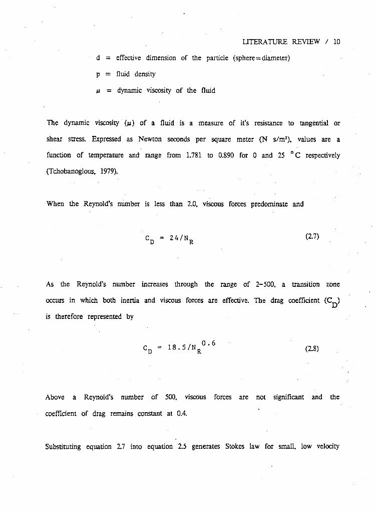
The dynamic viscosity (M) of a fluid is a measure of it's resistance to tangential or
shear stress. Expressed as Newton seconds per square meter (N s/mJ), values are a
function of temperature and range from 1.781 to 0.890 for 0 and 25 °C respectively
(Tchobanoglous, 1979).
When the Reynold's number is less than 2.0, viscous forces predominate and
C D = 24/N R (2-7)
As the Reynold's number increases through the range of 2-500, a transition zone
occurs in which both inertia and viscous forces are effective. The drag coefficient (C^)
is therefore represented by
C D = 1 8 . 5 / N R ° ' 6 (2.8)
Above a Reynold's number of 500, viscous forces are not significant and the
coefficient of drag remains constant at 0.4.
Substituting equation 2.7 into equation 2.5 generates Stokes law for small, low velocity

particles. Expressed as
UTERATURE REVIEW / 11
v = ( P s " P )gd 2
(2.9)
18>i
where V = terminal velocity of particle
P g = density of particle
p = density of fluid
g = acceleration due to gravity
M = dynamic viscosity of the fluid
d = particle diameter
The waste solids generated within a fish farm or hatchery are generally small, low
velocity particulates. It should therefore be expected that Stokes Law (Equation 2.9) can
be used to characterize their settling velocities.
Assuming this relationship to be correct, and the density and viscosity of the fluid to
be constant, the settling velocity of the particles will thus be a direct function of the
diameter and density of the particle. Any force which effectively alters either of these
two factors will therefore alter the settling velocity of that, particle.
The size and density of particulate solids discharged from a fish farm or hatchery has
been shown to be influenced by a variety of physical and site specific factors. These
include; the species and size of fish contained (Wheaton, 1977), the type (Stechey,
1986) and pellet size of feed used (Walden & Birkbeck, 1974), the retention time of
the waste within the containment unit (Warrer-Hansen, 1982) and by the amount of

LITERATURE REVIEW / 12
physical agitation and resuspension of the waste (Muir, 1978; Warrer- Hansen, 1979).
Warrer-Hansen (1979) reported settling rates for intact trout excreta to be generally
high and dependent on the weight of fish (Figure 2.1). Results of settling tests on
fresh excreta showed that on average, excreta from 20 gram fish settled at a rate of
3.3 cm/sec, while wastes from 5 gram fish settled at a lower rate of 1.7 cm/sec.
Wastes from fish less than 5 grams were shown to settle at a correspondingly lower
velocity. However, wastes which had been retained within the culture unit exhibited
much lower settling velocities (Querellou et al., 1982). This was illustrated by Walden
& Birkbeck (1974) who reported that wastes discharged from a hatchery exhibited two
major settling fractions. Over 50% of solid particulates had settling velocities faster than
0.2 cm/sec, while 40% had settling rates faster than 0.51 cm/sec. Both of these settling
velocities are significantly lower than those reported for fresh excreta (Warrer-Hansen,
1979).
It is assumed, and generally found that unless biologically or physio-chemically acted
upon, waste solids are dispersed and uniformly passed through the culture system.
However, waste solids often collect in areas of low velocity. The length of time a
waste solid may be retained in a holding unit will thus be a function of the tank
configuration, the velocity profile of the system, the degree of resuspension by fish
and mechanical aeration, and by the method and schedule of cleaning.
Once a particulate is trapped in the culture unit, it is subjected to a variety of
physical and chemical processes which can alter the particles physical characteristics.
Bacterial decomposition, hydration and physical shearing all act to reduce the particles

UTERATURE REVIEW / 13
FIGURE 2.1 Settling velocities for intact Rainbow trout excreta as a function of fish size (Warrer-Hansen, 1982)
1 1 0
C 2.0-
- 1.0
200 400 600 800
Size of trout ( no / Kg ) I I 1 1 L
1000
20 10 S>0 2.5 2SI 1,67 1.25 weight of trout ( g)
1.0

LITERATURE REVIEW / 14
size and density, thus reducing the settleability of the particle.
Warrer-Hansen (1982) summarized the results of settling trials on solid wastes
discharged from 3 tank configurations; an earthen pond (Warrer-Hansen, 1979), a
circular tank (Warrer-Hansen, 1979), and a tank of unspecified configuration (Muir,
1978), (Figure 2.2).
Warrer-Hansen (1979) observed that the wastes discharged from an earthen pond,
exhibited poor settling characteristics. This he concluded was due to the extremely long
retention times of solids within the tank, associated with the earth pond design. Low
velocities, long residence times of water within the pond and infrequent cleaning all
act to trap and hold waste solids for long periods of time. The waste solids are thus
subjected to extensive bacterial decomposition and hydration. Frequent resuspension by
fish during feeding, grading and harvesting, act to break up the solids into smaller,
less settleable fractions. It is therefore not suprising that removal rates of less than
50% are observed even after 30 minutes.
The second configuration reported by Warrer-Hansen (1979), the circular tank, appears
to provide conditions more conducive to rapid solids removal, as removal rates of 70%
were achieved after 30 minutes. Muir (1978) reports complete solids removal (100%)
after 40 minutes in wastes discharged from the unspecified tank configuration. However,
assuming that conditions under which the waste solids were produced were the same
(feed type, feed pellet size, fish size), the circular tank would be more desirable.
Figure 2.2 illustrates two distinct settling patterns. In both tank configurations reported

LITERATURE REVIEW / 15
FIGURE 2.2 Relationship between residence time and solids removal (Warrer-Hansen. 1982)

LITERATURE REVIEW / 16
on by Warrer- Hansen (1979), the bulk of solids removal occurred within the first 15
minutes of settling, after which time there was a gradual decline in the rate of
removal with time. However, the curve reported by Muir (1978), shows that the bulk
settling of settleable solids (>60%) occurs between 15 and 20 minutes after settling has
begun. This would indicate that the wastes solids are relatively uniform in size and
density, but lighter or smaller than wastes reported in Warrer-Hansen (1979). Although
the circular tank configuration does not ultimately achieve the same level of removal
(100%) as Muir (1978), it does achieve comparable levels of removal (below 70%) in
significantly shorter residence times.
This is desirable for two reasons: 1) rapid solids removal reduces the residence time
required to achieve a desired level of removal, which reduces the size of the gravity
solids separation system and consequently the capital and operating costs of the system,
2) rapid solids settling reduces the need for totally quiescent conditions within the
clarifier. This effectively reduces the potential for resuspension of the waste solids
which may occur as a result of occassional turbulence within the treatment system.
Walden & Birkbeck (1974) reported that feed type and pellet size also influenced the
settleability of the wastes produced. Although no specific data was introduced to
quantify any differences between feed types, they did provide more specific results on
pellet size. It was observed that wastes produced from fish fed 3/32 inch dry pellets,
achieved 48-68% solids removal within the first 5 minutes, while wastes from fish fed
a finer (grower crumbles) pellet size, took longer (15 minutes) to achieve similiar
removals (55%).

LITERATURE REVIEW / 17
In a recent study involving settling column analysis of a raceway cleaning effluent
from an Ontario trout farm using Martins ® dry pellet feed, Stechey (1986) reports
that effluents, with initial solids concentrations of 300-500 ppm, achieved 50% solids
removal within 20 minutes. However, 60 minutes was required to obtain 65% solids
removal.
The mode and length of time between cleanings, and the method of solids handling
has also been shown to influence settleability. In a report prepared by Hydroscience
Inc.(1977) on wastewater treatment and control in Idaho hatcheries, it was observed
that cleaning operations employing vacuums or pumps for handling wastes, produced
wastes of poor settleability. It was further observed that if pumps were to be used,
then diaphragm type pumps should be employed as they minimized solids break-up.
Given the wide range of factors which influence the physical nature of the wastes and
their subsequent settleability, it is not surprising that there is wide variation in
reported clarifier design and treatment efficiency. A number of overflow rates and
residence times have been reported in the literature as providing treatment for fish
culture wastes. Liao & Mayo (1974) report that an overflow rate of 49,000 1/mVday,
with a retention time of 15-30 minutes was adequate for treatment Walden &
Birkbeck (1974) reported that a retention time of 8-15 minutes at an upflow rate of
6.8-9.2 mVmVday (converted from gal/ftVday) was sufficient to reduce suspended
solids and BOD by 37-52% and 16% respectively. Sparrow (1981) reported that a 12
minute retention time in a 0.46m deep settling basin was sufficient to remove 90% of
settleable solids. Bergheim and Selmer-Olsen (1978) suggested a medium retention
period of 20 minutes would be sufficient to achieve satisfactory settling. Petit (1978)

LITERATURE REVIEW / 18
reported suspended solids removal of 92% after 30 minutes. Muir (1978) reported 66%
of solids settled within 5 minutes while 90% settled within 15 minutes.

3. THEORY
A clarifier or sedimentation basin is designed for a particular waste by selecting a
suitable settling velocity (V ) such that all particles with settling velocities greater than o
V q will be removed. The rate at which clarified water is produced can then be
expressed as (Tchobanoglous, 1979)
Q = A V Q (3.1)
where Q = flow rate (mVday)
A = surface area of clarifier (m2)
V = settling velocity of waste particle (m/day) o
Rearranging equation 3.1 for V q (Equation 3.2)
3 2 V q = Q/A = o v e r f l o w r a t e (m /m /day) (32)
shows that the overflow rate or surface loading rate, is equivalent to the settling
velocity (Figure 3.1).
From the geometry of Figure 3.1, it can be seen that if the area of the triangle,
having legs H and L, represents 100% removal of particles, then the removal or
particles having settling velocities less than V ( V ) will be in the ratio h/H. Given o s
the depth a particle will settle is equal to the product of the settling velocity of that
particle, and the retention time (t ), then the ratio at which particles with settling
19

THEORY / 20
FIGURE 3.1 Schematic of an ideal rectangular sedimentation basin, indicating the settling path of discrete particles
Surface area A-bL
Inlet
Inflow«Q
Out flow«Q outlet weir

THEORY / 21
velocities less than V will be removed will be o
, V t V ^ = - L - - ^ = _ - i _ (3.3)
H V t V o o o
The efficiency of a sedimentation basin is a measure of the removal of suspended
solid particulates at a given overflow rate V . From the discussion and observation of
Figure 3.1, for a clarification rate of V , it has been shown that those particles o
having settling velocities greater than V q will be completely removed. The fraction of
particles removed from the suspension will thus be 1-C .where C represents the o o
fraction of particles with settling velocities less than V . However, for each size o
particle with a settling velocity less than V , it has been shown that the fraction o
removed would be equal to the ratio of V /V . Therefore, when considering the s o
efficiency of the sedimentation basin for removing particles within this category, the
percentage removal of these particles is given by (Clark et al, 1977)
f °
0
V s (3.4) dc
V o
The overall removal of suspended solids in a clarifier with a designed overflow rate
of V is thus determined using equation 3.5. Expressed as a total percent removal o
T o t a l % Removal = ( 1 - C ) + o
V G
d s • (3.5)
V C
o' where C = fraction of particles having settling velocities less than V o o

THEORY / 22
Equation 3.5 is generally solved by integration of the area between 0 and a selected
overflow rate (V ) on the particulates settling velocity distribution curve (Figure 3.2).
Figure 3.2 can be derived in two ways; 1) by selective sieve analysis and hydrometer
tests in combination with Newton's Law (Equation 2.5), or 2) using settling column
analysis of the waste. For the purpose of continuity of discussion, the application of
method 2 will be described during the discussion of Type II settling and the
derivation of the Type II or flocculant particle settling curve.
The overflow rate (V ) is subsequently chosen such that the desired percentage of
suspended solids removal can be achieved. However, this design procedure is only
effective if the waste solids conform to Type I or discrete particle settling only.
In Type I settling, each particle behaves as an individual entity and settles at a
uniform rate determined by equations 2.1-2.9. The particle is said to follow a linear
path, illustrated in Figure 3.3.
Chesness et al. (1975) observed that fish culture wastes exhibited two forms of settling
behavior. In effluents of low suspended solids concentrations, like those produced during
normal hatchery operations, Type I settling predominates. However, during cleaning and
feeding operations, suspended solids concentrations can increase to levels where
particulates begin to collide and coalesce, assuming the settling velocity of the new,
larger or heavier particle. The particles exhibiting Type II or flocculant settling will
thus follow a curvlinear path as illustrated in Figure 3.4.

THEORY / 23
FIGURE 3.2 Discrete particle velocity cumulative frequency distribution

THEORY / 24

THEORY / 25
The degree to which coalescence or agglomeration may occur will be due in part to
the opportunity for contact between particles. This in turn is related to a number of
factors, including; the suspended solids concentration, the range of particle sizes present
in the waste, the distance the particles are to settle, and the velocity gradient within
the system.
In Type I settling, the overall solids removal efficiency is a function of the overflow
rate only and independent of the depth of the clarifier. However, in Type II settling,
where particle interaction will be a function of depth and time, retention time and
clarifier depth must also be considered when determining solids removal efficiency.
Given the high level of particle interaction in Type II settling, the necessary design
parameters can no longer be set on the basis of a simple mathematical relationship as
in Type I settling. Overall suspended solids removal efficiency can presently be
determined by empirical methods only. This is accomplished using a settling column
equal in height to the clarifier depth, and of at least 15 cm in diameter
(Tchobanoglous, 1979).
The settling column is used to approximate conditions within a clarifier in order to
produce a graphical representation of the rate of solids removal as a function of time
and depth. Effluent samples collected from the settling column are analyzed for
non-filterable residue and subtracted from the initial non-filterable residue concentration
in order to determine the level of removal of non-filterable residue over time.
Expressed as a percentage of the initial concentration, the level of non-filterable
residue removed, is plotted as a function of residence time and sample port depth.
With the inclusion of iso-concentration curves, representing points of equal levels of

THEORY / 26
removal, the Type II or flocculant particle settling curve is obtained (Figure 3.5).
The overall level of solids removal, within the column, at a specific residence time
(T), is then determined by integrating the percent solids removal over the height of
the column using equation 3.6.
Overall % ^ h l W + &h<W + " ^ V V W solids - 2 2__ 2 removal . . , , A , . A , . v ' ( A h , + A h 0 + . . . Ah ) l z n
where A hn ( R
n+ R
n + i ) = average solids removal concentration within a section of ~~2
the column depth h.
As an example to illustrate the use of equation 3.6, the overall non-filterable residue
removal concentration will be determined from Figure 3.5 for a residence time of T2.
For the example shown in Figure 3.5, equation 3.6 may be rewritten as
A (90+80) + A h 2 (80+70) + Ah3(70+60) + Ah (6(H50) ( 3 ? )
hJT ~~2 h5 ~2 h5 2 h 5 ~2
where hj = height of the seuling column

THEORY / 27
FIGURE 3.5 Type II or flocculant particle settling curves (Note: Percentage
removal curves (R ) are interpolations of the solids fraction removed n
as a function of residence time and column depth)
Time ( m i n u t e s )

THEORY / 28
Results of the computations are summarized in Table I
TABLE I Summary of integration calculations of flocculant particle removal for a residence time T 2
h x R +R ,, = Percent Removal n n n+l
h 5 0.10 x (90+80) = 8.5
2
0.10 x (80+70) = 7.5 2
0.13 x (70+60) = 8.45 2
0.67 x (60+50) = 36.85 2
1.00 T o t a l % Removal =61.3
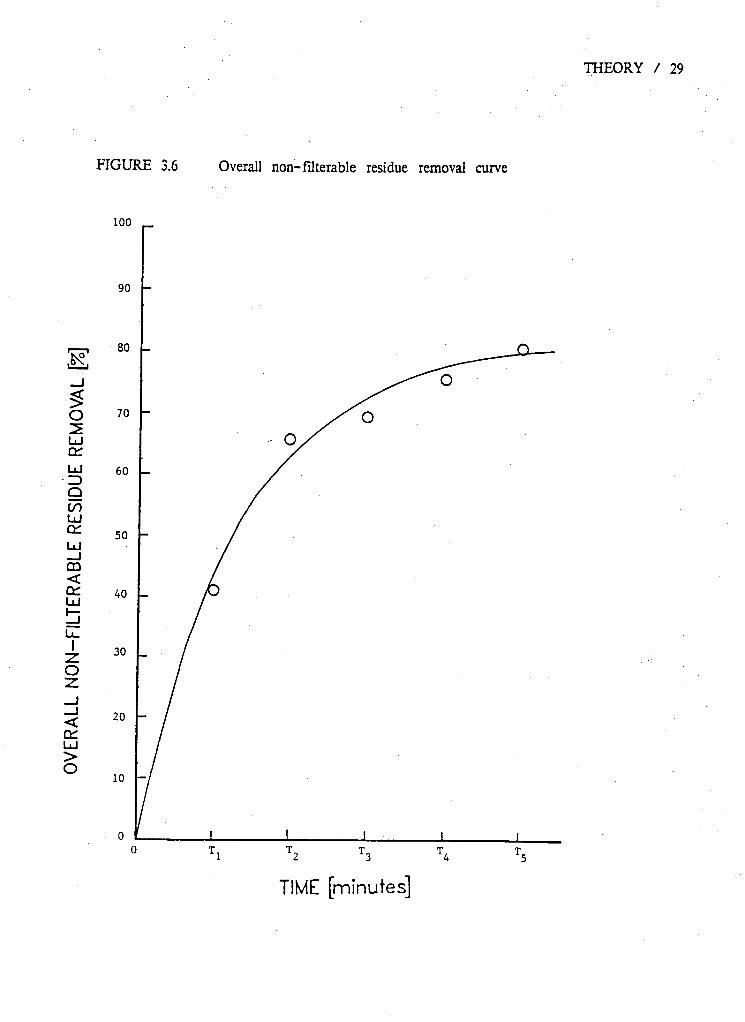
Continuing this integration for each unit of time, thus provides a graphical
representation of the level of solids removal as a function of residence time (Figure
3.6). The solids removal curve illustrated in Figure 3.6 is then used in sizing the
clarifier by selecting the residence time required to achieve the desired % solids
removal.
As previously discussed, the settling column may also be used to derive the individual
particle settling velocity distribution curve.
The isc—concentration curves on the Type II settling curve represent lines or points of
equal levels of non-filterable residue removal. However, they also represent the
maximum trajectories of particle settling paths for a specific concentration in a
flocculant suspension. For example, in Figure 3.5, 60% of the particles will have
THEORY / 29
FIGURE 3.6 Overall non-filterable residue removal curve
100 _
O UJ a: U J •ZD Q
CO U J
U J _ J CD < OH U J
< U J > o
TIME [minutes]

THEORY / 30
velocities greater than h2/T2 at the time the particles reach a depth of h2. Simplified,
the curve shows that for a particle to be removed from the column, it's settling
velocity must be greater than the depth to be traversed (h2) divided by the allowed
time or residence time (T2). Therefore for the same example, the curve shows that
50% of the particles have settling velocities greater than h5/T2 ( V ) and will therefore o
be removed. However, within our discussion of discrete particle settling, it was shown
that particles with settling velocities less than V Q ( V ) will be removed in the ratio of
V / V . The overall level of removal as a function of settling velocities is therefore s o
obtained by integration of the Type II settling curve using equation 3.5. Where 1 -
C q represents the percentage of solids with settling velocities greater than V q (h /T ).
The second term within equation 3.5 therefore represents the fraction or percentage of
particles with settling velocities V less than which are removed.
The total fraction of particles which are removed with settling velocities greater than,
equal too and less than h /T ( V ) is ^ t o o
( 1 - c o ) + V W + _ V W + ••• h i < V i - V <18>
Where 1 - C = fraction of particles removed at the maximum depth (h ) of
the settling column given a residence time T : 0
h = total depth of settling column or clarifier
h = depth within the column at vertical midpoint between particle n
trajectory curves R and R , n n-1
In Figure 3.5 the fraction of particles removed at a residence time of T2 is expressed

THEORY / 31
as
50 + h4(60-50) + M70-60) + h?(80-70) + hi (90-80) — — —± — (3.9) h 5 h 5 h 5 h 5
However, this calculation has already been indirectly solved in the derivation of the
overall non-filterable residue removal curve. The overall non-filterable residue removal
curve is a graphical representation of the level of solids removal as a function of
residence time. Restated, this curve is a representation of the percentage of particles
with settling velocities greater than h /T . Figure 3.6 may therefore be rearranged as
the percentage of non-filterable residue with settling velocities greater than h / T t o
(Figure 3.7).
The individual particle settling velocity distribution curve can therefore be obtained
from Figure 3.7 by plotting the residual of 1 - (the fraction of non-filterable residue
with settling velocities greater than h/T ), to obtain the fraction of non-filterable t o
residue with settling velocities less than h /T (Figure 3.8).

THEORY / 32
PARTICLE SETTLING VELOCITY

F I G U R E 3.8 Ind iv idual part ic le sett l ing veloc i ty d is t r ibut ion curve
PARTICLE SETTLING VELOCITY

4. MATERIALS AND METHODS
4.1. SPECIES
Rainbow trout (Salmo gairdneri) were selected for use in this study as representative
of the family of salmonids presently raised in British Columbia. The selection of the
species was based primarily on two factors; 1) the entire life cycle from egg to
market, occurs in fresh water, 2) Rainbow trout are grown extensively in the Lower
Mainland for both the commercial and sports fishery markets. The species was
therefore readily available at all times and in the sizes required. Rainbow trout were
obtained from two sources; Fraser Valley Trout Hatchery (Ministry of Environment,
Fish and Wildlife Branch) and Spring Valley Trout Farm.
4.2. FISH SIZE
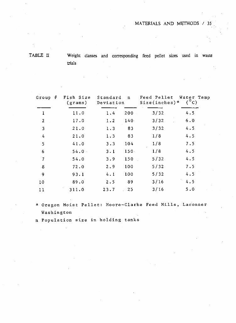
Uniform populations were chosen on the basis of weight Weight classes were selected
from the feed manufacturers feeding guide to provide waste trials for the lower,
middle and upper range of fish sizes recommended for each pellet size used. Table II
summarizes the pellet sizes used, and the corresponding weight classes. The use of
three weight classes for each pellet size used was chosen to provide a means of
comparing the effects of weight on waste solid settling rates, independent of pellet
size. Overlap of weight classes amongst pellet sizes, provided a means of comparing
the effects of pellet size, on waste settling rates, independent of weight The weight
sizes used in the study ranged from 11 to 311 grams.
34
MATERIALS AND METHODS / 35
TABLE II Weight classes and corresponding feed pellet sizes used in waste trials
Group // F i s h S i z e S t a n d a r d n F e e d P e l l e t W ater (grams) D e v i a t i o n S i z e ( i n c h e s ) * (°C)
1 11.0 1.4 200 3/32 4.5 2 17.0 1.2 140 3/32 6 . 0
3 21.0 1.3 83 3/32 4.5 4 21.0 1.3 83 1/8 4.5
5 41.0 3.3 104 1/8 7.5 6 54.0 3.1 150 1/8 4.5
7 54.0 3 . 9 150 5/32 4.5
8 72.0 2.9 100 5/32 7.5
9 93. 1 4.1 100 5/32 4.5
10 89 .0 2.5 89 3/16 4.5
11 311.0 23 . 7 25 3/16 5.0
* Oregon M o i s t P e l l e t : M o o r e - C l a r k e F e e d M i l l s , L a c o n n e r W a s h i n g t o n
n P o p u l a t i o n s i z e i n h o l d i n g t a n k s

MATERIALS AND METHODS / 36
4.3. FEED TYPE AND PELLET SIZE
Oregon Moist Pellet ®, produced by Moore-Clark, was used in the feed-waste trials.
The fish in each weight class were fed the feed pellet size, at a rate recommended
by the manufacturers feeding guide. The feed was distributed on a daily basis over a
15 hour period in 8 equal portions by means of an automated type feeding system.
The pellet sizes used in the feed-waste trials, as summarized in Table II, were the
3/32, 1/8, 5/32, and 3/16 inch pellet
4.4. LABORATORY SET UP
4.4.1. Containment
Each test population was held in 200 litre (50 gallon) oval fibre glass tanks (Figure
4.1) which were obtained from the Department of Fisheries and Oceans West
Vancouver Marine Laboratory. Each tank was equipped with a 10 cm (4 inch) central
standpipe drain which regulated the water level within the tank and reduced the
discharge of settled waste solids.
4.4.2. Water Supply
Each tank was provided with dechlorinated water through an over-head pipe. Overall
flow rates were controlled at the main supply level by means of a constant head
tower. Individual tank flow rates were maintained using a 1.3 cm (1/2 inch) ball
valve.
Water temperature ranged from 4 °C to 7 °C during the course of the study.
Flow rates for each test population were based on two factors; 1) the minimal flow
MATERIALS AND METHODS / 37
FIGURE 4.1 Schematic of 200 litre fibre glass tanks

MATERIALS AND METHODS / 38
rate required to prevent scouring of the tank bottom and loss of solids, and 2) the
minimal flow rate required to maintain suitable water quality within the holding tanks.
4.4.3. Aeration
Aeration was provided at the main constant head tower, and at each 200 litre tank
using a venturi aspirator attached to the 1.3 cm (1/2 inch) valve. Aeration was
maximized at the air/water interface of the water jet stream by adjusting the angle of
the water stream from the aspirator to 60 0 (from the horizontal)(Chesness et al,
1973).
4.4.4. Stocking Density
Stocking densities were selected on the basis of; 1) the number of fish available
within the size range desired, and 2) the number of fish in a particular size class
required to produce a measurable quantity of waste solids.
4.5. SETTLING COLUMN
A plexiglass column, 230 cm in height by 15 cm in diameter was used in the settling
rate trials. The column was equipped with 7 sampling portes, located, starting at 22
cm from the bottom of the column and then continuing up the column at 30.5 cm
intervals (Figure 4.2 ).
Pressurized air was supplied to the base of the column to provide mixing.

MATERIALS AND METHODS / 39
FIGURE 4.2 Schematic of settling column used in settling trials
Dimensions in centimeters (cm)
Set t l i n g column inside diameteT"
15.0 cm
T 30.5
3 -+«
sampling port
30.5
2
30.5
22.0
T 30.5
30.5
30.5
217 230

MATERIALS AND METHODS / 40
4.6. EXPERIMENTAL PROCEDURE
Weight classes were acclimatized to the feed and pellet sizes for a period of three
days prior to waste collection. This was carried out to insure that the wastes produced
were of the pellets being fed, and to insure that the fish were feeding normally.
The tanks were thoroughly cleaned of any accumulated solids prior to waste solids
collection. The solid wastes were then allowed to accumulate over a 24 hour period.
During this 24 hour period, the fish were fed according to the program outlined in
Section 4.3. At the end of the 24 hour period, the settled solids were collected from
the tank and placed in the settling column. Collection of the settled waste solids from
the bottom of the holding tanks was carried out using a modified vacuum siphon
tube. A modified 2x2x2 cm (3/4x3/4x3/4 inch) T-fitting, attached to the end of the
siphon hose produced a configuration similiar to the floor wand of a vacuum cleaner .
This increased the functional area of the siphon and reduced turbulence. The large
diameter of the tubing used in the siphon, and the low vacuum pressures used also
prevented the fragmentation of the fecal pellets and unconsumed feed pellets.
To minimize the shear forces inherent in transfering the collected waste solids from
the collection buckets to the settling column, the column was first partially filled to a
depth of 180-200 cm with clarified effluent from the collection buckets. The settled
solids were then added to the column. Rinse water from the collection buckets was
used to bring the total column depth to 217-220 cm.
Mixing of the effluent within the column was accomplished using the compressed air
system, located at the base of the column. The release of compressed air at the
MATERIALS AND METHODS / 41
bottom of the column produced conditions similiar to an air lift pump. The use of
the air lift pump system for mixing did not appear to effect the particle sizes.
Although care was taken, during the collection and manipulation of the waste solids, to
minimize particle fragmentation, it must be assumed that in a hatchery or farm
situation, fragmentation of fecal pellets and unconsumed feed pellets will occur. This is
unavoidable as the solid particulates are subjected to shear forces during mechanical
aeration and as the waste effluent cascades through a series of raceways or ponds.
Two sets of 100 ml samples were taken from each sampling port during mixing as a
test for uniformity, and to provide a baseline concentration from which further samples
would be compared. Mixing was terminated immediately after the last mixing sample
was taken.
After termination of aeration, 100 ml samples were then collected from each sample
port at 1, 3, 6, 15 and 30 minute intervals. A final 200 ml sample was taken from
each port at 60 minutes.
Each sample taken from the column was then filtered through preweighed 5.5 cm
Whatman ® glass fibre filters (934-AH). The filters and non-filterable residue were
then dryed at 105 °C for 24 hours.
After 24 hours the filters and residue were removed from the drying oven and placed
in a desiccator to cool, after which time they were weighed and the amount of
non-filterable residue determined.

MATERIALS AND METHODS / 42
The two sets of samples collected during mixing were pooled and an average taken in
order to provide a baseline or starting concentration from which the level of
non-filterable residue removed would be obtained. The level of non-filterable residue
removed in each sample was calculated as the difference between this initial
non-filterable residue and the amount of non-filterable residue present on each of the
sample filter papers. The level of non-filterable residue removed, expressed as a
fraction or percentage of the baseline or starting concentration was then plotted as a
function of residence time and sample port depth to provide the framework for the
Flocculate particle or Type II settling curve illustrated in Figure 3.5. The Type II
settling curves were then used in the derivation of the overall non-filterable residue
removal curves and the individual particle settling velocity distribution curves as
outlined in Chapter 3.
The sampling procedure used in this study differed from the standard methods
reported in the literature, in that no makeup water was added to the column after a
sample was taken. This modification required that a variable column height be used
when calculating settling velocities from the Type II settling curve.

5. RESULTS AND DISCUSSION
Non-filterable residue removal curves and individual particle settling velocity distribution
curves are used to characterize a waste solids settling behavior. These curves were
selected for use in this study as a means of evaluating and comparing the effects of
Fish size and feed pellet size on the settleability of the waste solids produced.
Although the study deals primarily with waste produced during the feeding of a moist
pellet diet, similiar trials were carried out using a dry pellet feed (Purina Trout Chow
®), and will be discussed where appropriate.
In producing the non-filterable residue removal curves and individual particle settling
velocity distribution curves to be presented in this study, a number of assumptions
were made. Waste solids produced from the feeding trials were allowed to accumulate
in the holding tanks over a 24 hour period prior to collection and analysis. During
this time, the waste solids, composed of faeces and unconsumed feed pellets, were
subjected to hydration and physical shearing. These two processes, combined with
periodic resuspension of the solid particulates, resulted in the breakup of solid
particulates and the loss of some solids. Due to the arrangement of the tank
discharge, and the large volumes of water used, it was not possible to determine the
quantity or sizes of the waste solids lost However, it was assumed that under actual
operating conditions these same solids would be lost through resuspension. They would
therefore form part of the average daily waste loading of the farm. As this study was
concerned primarily with the treatment of the significantly higher strength cleaning
flows (Liao, 1970; Bergheim et al, 1984), we were interested in only that fraction
which was retained within the culture unit The waste solids lost through resuspension
were therefore ignored.
43

RESULTS AND DISCUSSION / 44
Initially the study proposed to evaluate, in addition to fish size and feed pellet size,
the effect of feed type on the physical characteristics of the waste produced. Two
feeds were selected which represented alternate milling processes; 1) a frozen feed
(Oregon Moist Pellet ®), produced by Moore-Clark and 2) a dry pellet (Purina Trout
Chow ®) produced by Ralston Purina.
In feeding trials using the Oregon Moist Pellet ® feed, sufficient solids were retained
within the tanks to produce the desired solids removal and particle settling velocity
distribution curves. However, in trials using the dry pellet feed, of the three pellet
sizes used, only the #4 size produced any measurable quantity of waste solids. In
trials using the #3 and #5 pellet sizes, most of the solids were lost Those solids
which were retained, only after severely restricting water flow through the tanks,
tended to form a gelatinous mat which adhered to the tank bottom and discharge
screens.
It was also observed that in trials using the #4 pellet, a large quantity of yellowish
grit was found to collect in the tank. This may have been undigested corn particulates
or part of the vitamin premix.
Due to this inability to obtain consistent measurable quantities of waste solids, it was
decided to terminate further studies using the dry pellet feed.
Once the accumulated waste solids had been collected, they were placed in the settling
column for analysis. The column simulates a portion of a clarifier or sedimentation
basin. Sampling ports located along the side of the column allow for samples of the

effluent to be withdrawn for analysis.
RESULTS AND DISCUSSION / 45
The settling column can be used to derive the non-filterable residue removal and
individual particle settling velocity distribution curves used in this study provided two
conditions are met; 1) the waste solid particulates are uniformly distributed within the
column, and 2) quiescent conditions exist in the column during sampling.
Waste solids were kept in suspension within the column using compressed air.
Compressed air was released at the bottom of the column and allowed to rise through
the column, creating conditions similar to an air lift pump. The bubbles produced were
kept large to reduce air flotation of the waste particulates. In this process, small
bubbles adhere to the solid particles in suspension, producing lift The solids
subsequently float to the surface where they collect as a foam or scum. However,
even with the large bubbles used some flotation of small solid particulates was
observed. Once aeration was terminated , small low velocity waste solid particulates
continued to rise, forming a scum at the surface of the column. No attempt was
made to quantify the amount of solids removed by this process, as agitation of the
layer resulted in it's breakup and settlement It is assumed however that in review of
the high rate of settleable solids removal observed within the first 5-8 minutes (Figure
5.5 - 5.15), the air flotation removal of these low density particulates does not
contribute significantly to the overall rate of removal during this period. The inclusion
of these particulates only slightly reduces the slope of the overall non-filterable residue
removal curve during the first 5-8 minutes of settling.
As a test for uniformity of waste solids within the column, two sets of samples were

RESULTS AND DISCUSSION / 46
collected from each sampling port during mixing of the waste effluent From this set
of samples it was observed that there was a high degree of variability in the
concentration of suspended solids within the column (Table III). In general, suspended
solids concentrations increased from the top of the column, down to the bottom. A
general decline in the overall level of suspended solids within the column over time
was also observed. Both of these observations indicated that some settling of solids was
occurring during mixing. However, increasing the level of aeration to over come this
settling, resulted in loss of the waste water out of the top of the column. It was
decided therefore that some settling of solids was unavoidable.
For the purpose of this study, a mean of the twelve samples taken during mixing, as
shown in Table III, was used as the initial solids concentration or baseline
concentration. However, using a mean value in the percent removal calculations to
represent a column with varying suspended solids concentrations provided some error in
the values obtained. At the top of the column, actual solids concentrations will be
higher than the mean used, therefore the percentage of solids removal calculated from
the samples taken from this region will be overstated. However, the opposite is true
for the lower portion of the column. The use of a mean suspended solids
concentration will underestimate the actual percentage of solids removed.
Given that the non-filterable residue removal curves reflect the rate of removal within
the entire column, small localized variations will tend to be buffered out To minimize
the possible spread between the mean concentration used in our calculations and the
actual initial solids concentration, sampling for the settling trials was begun immediately
after the last mixing samples were taken.

RESULTS AND DISCUSSION / 47
TABLE III Variability of initial non-filterable residue concentrations as a function
of column depth
T r i a l I T r i a l I I Sample P o r t * Sample 1 Sample 2 Sample I Sample 2
(grams) (grams) (grams) (grams) 1 0.0631 0.0582 0.0629 0 .0754 2 0.0689 0.0598 0.0720 0.0654 3 0.0583 0.0474 0.0665 0.0604 4 0.0540 0.0472 0 . 065 1 0.0620 5 0.0550 0.0455 0.065 1 0.0614 6 0.0503 0.0432 0 . 0624 0 .0626
X = 0 .0542 X = 0 .065 1 S = 0 .0078 S = 0 .0045
I n i t i a l C o n c e n t r a t i o n 542 mg/l 651 mg/: * R e f e r to F i g u r e 4.2 f o r s e t t l i n g column sample p o r t
l o c a t i o n Note: N o n - f i l t e r a b l e residue i n T r i a l I and T r i a l II i s based on
sample volume of 100 ml.

RESULTS AND DISCUSSION / 48
The second requirement in running settling trials in the column is that quiescent
conditions be maintained within the column. The settling column was located in the
fish culture lab, which due to the high volumes of water contained in the holding
tanks, maintained an ambient temperature equal to the incoming water. The effluent
placed in the column was therefore free of any external temperature gradients, and the
convection currents which are produced when a gradient exists.
Some minor upwelling was observed at the start of the settling trials as a result of
the air lift pump mixing system used. However, this was generally of short duration.
The column was observed to be quiescent within 5 to 7 minutes after termination of
aerated mixing.
Given that the waste solid particulates were uniformly distributed within the column,
and that the column was quiescent, the settling column can be used to approximate
conditions within a clarifier or settling basin. Samples collected from the column can
thus be used to derive the Type II or flocculant particle settling curves for the waste.
The flocculant particle settling curve can in turn be used to obtain the overall
non-filterable residue removal curve and the individual particle settling velocity
distribution curve for the waste.
As previously discussed, the two sets of samples collected during mixing were used to
determine the baseline initial non-filterable residue concentration within the settling
column (Table III). Samples collected after termination of mixing were then measured
for non-filterable residue and compared to the initial concentration to determine the
level of non-filterable residue removed over time (Table IV). The level of

RESULTS AND DISCUSSION / 49
TABLE IV Non-filterable residue concentrations for a sample settling trial
imple Sample P o r t N o n - F i l t e r a b l e Z Removal R e s i d e n c e # L o c a t i o n * R e s i d u e (grams) Time (min)
1 1 0.0399 26.4 1 :00 1 2 0 .0432 20.3 1 3 0.0381 29 .7 1 4 0.0349 35 .6 1 5 0.0410 24.4 1 6 0.0282 48.0 2 1 0.0297 45 .2 3:00 2 2 0.0305 43.7 2 3 0.0296 45 .4 2 4 0.0262 51.7 2 5 0.0285 47.4 2 6 0.0209 61.4 3 1 0.0243 55 .2 6 :00 3 2 0.0242 55 .3 3 3 0.0207 61.8 3 4 0.0168 69.0 3 5 0.0167 69.2 3 6 0.0121 77 . 7 4 1 0.0143 73.6 15 :00 4 2 0.0142 73.8 4 3 0.0135 75 .1 4 4 0.0119 78.0 4 5 0.0108 80. 1 4 6 0.0085 84.3 5 1 0.0100 81.5 30 :00 5 2 0.0114 79 .0 5 3 0.0103 81.0 5 4 0.0094 82 .7 5 5 0.0075 86 .2 5 6 0.0062 88.7 6 1 0.0071 86 .9 60:00 6 2 0.0074 86 .3 6 3 0 .0077 85 .8 6 4 0.0079 85 .4 6 5 0.0070 87 .1 6 6 0.0069 87.3
* R e f e r t o F i g u r e 4.2 f o r l o c a t i o n of s e t t l i n g column s a m p l i n g p o r t
RESULTS AND DISCUSSION / 50
non-filterable residue (X ), expressed as a percentage, was then plotted as a function o
of column depth and residence time in order to provide the frame work for the Type
II settling curves (Figure 5.1). With the inclusion of iso-concentration lines, representing
points of equal levels of non-filterable residue removal, the Type II or flocculant
particle settling curve was obtained (Figure 5.2).
The Type II settling curve (Figure 5.2) thus provided a graphical representation of the
level of solids removal over time at various depths within the settling column.
However, to be of use as a design tool, it was necessary to know what the overall
level of solids removal was for the entire column. This was obtained from the Type
II curve by integration of the various iso-concentration curves using equation 3.6 as
outlined in Chapter 3. Plotting of the resulting overall non-filterable residue removal
concentrations for each unit of time resulted in the overall non-filterable residue
removal curve (Figure 5.3).
The individual particle settling velocity distribution curve was in turn obtained by
plotting the residual of 1-X , where X is the level of overall non-filterable residue o o
removed at a residence time T (expressed as a fraction), against the particle settling o
velocity as outlined in Chapter 3. Figure 5.4 illustrates the resulting individual particle
settling velocity distribution curve from the example data provided in Table IV.
Overall non-filterable residue removal curves (Figure 5.5 - 5.15) and individual particle
settling velocity distribution curves (Figure 5.16 - 5.26), were subsequently derived for
each of the test groups summarized in Table II.

RESULTS AND DISCUSSION / 51
FIGURE 5.1 Percentage of non-filterable residue removed as a function of residence time and column depth for data given in Table III
6*-| 61.4 77.
+ + + |48.0
5 "4 47.4 69.
+ + + 124.4
33 H CU w a 5= , * s 4 i S3
o cj
z •J H H W cn
3*4
+ [35. &
5^1.7 _IS9.0
69.7
61.8
60. 3
. 45.2 55.2 H - 4 - 4 — 26.4 1 3 6
84.3 +
80.1 +
78.0
73.8
73.6
- + -
15
i .7 +
86.2 +
82.7 ,
81.C
79. C
81.5 —4-30
RESIDENCE TIME (minutes)
87.3
+
87.1
85 .4 +
83.8
86.3
86.9
- 4 -60
* R e f e r t o F i g u r e 4 . 2 f o r s a m p l e p o r t l o c a t i o n a n d d e p t h

RESULTS AND DISCUSSION / 52
FIGURE 5.2 Type II or flocculant particle settling curves for example data in Table IV
26.4 1 3 6 15 30
RESIDENCE TIME (minutes)
* R e f e r t o F i g u r e 4.2 f o r sample p o r t l o c a t i o n and d e p t h

RESULTS AND DISCUSSION / 53
FIGURE 5.3 Overall non-filterable residue removal curve for example data in Table IV
O U J
cc
Q 00 UJ cc U J _ J m < cc U J
O
< cc U J > O
100-1
aoH
60 A
40
20 A
/ /
• A" . -A"
10 20 30 40 ~ r ~ 50 60 70 80
TIME [minutes]

RESULTS AND DISCUSSION / 54
FIGURE 5.4 Individual particle settling velocity distribution curve for example data in Table IV
x 1". z < X
o.a-\
A /
/
A / /
/ A
1 2 3 4 PARTICLE SETTLING VELOCITY [cm/sec]

RESULTS AND DISCUSSION / 55
FIGURE 5.5 Overall. non- filterable residue removal curves for 11 gram Rainbow trout fed 3/32 OMP feed pellets
(NoterLegend indicates initial non-filterable residue concentrations)
> o
0 Q 1 1 1 1 1 1 r 0 10 20 30 40 50 60 70 80 TIME [minutes]

RESULTS AND DISCUSSION / 56
FIGURE 5.6 Overall non-filterable residue removal curves for 17 gram Rainbow
trout fed 3/32 OMP feed pellets
(Note: Legend indicates initial non-filterable residue concentrations)
100-1
v i 1 1 1 1 1 1 0 10 20 30 40 50 60 70
TIME [minutes]

RESULTS AND DISCUSSION / 57
FIGURE 5.7 Overall non-filterable residue removal curves for 21 gram Rainbow trout fed 3/32 OMP feed pellets (Note: Legend indicates initial non-filterable residue concentrations)
100-,
Legend O 1007 m g / l s
A 676 m g / l
X 179 m g / l s
126
91
25
-T— 40 60 50 70
TIME [minutes]

RESULTS AND DISCUSSION / 58
FIGURE 5.8 Overall non-filterable residue removal curves for 21 gram Rainbow trout fed 1/8 OMP feed pellets
(Note: Legend indicates initial non-filterable residue concentrations)
O
UJ OH U J Z D Q CO U J OH
CD < OH
< OH U J >
o
6 0 -
4 0 -
2 0 -
•A
Legend O 9 0 3 m g / l s = 135 A 7 9 4 m g / l s = 9 8
X 5 8 4 m o ^ l s . A 5
10 20 30 40 TIME [minutes]
50 60 70

RESULTS AND DISCUSSION / 59
•FIGURE 5.9 Overall non-filterable residue removal curves for 41 gram Rainbow trout fed 1/8 OMP feed pellets
(Note: Legend indicates initial non-filterable residue concentrations)
I O O - I
O UJ OH
Q 00 UJ OH
< OH U J > O
80H
60 H
< OH y 4 o - i
20 H
Op-0 10
Legend O 1755 mg/l s
A 1148 mg/l s
X 422 mg/l s
• 329 mg/l s
186
132
39
60
20 30 40 50 60 TIME [minutes]
-1 70
RESULTS AND DISCUSSION / 60
FIGURE 5.10 Overall non-filterable residue removal curves for 54 gram Rainbow
trout fed 1/8 OMP feed pellets
(Note: Legend indicates initial non-filterable residue concentrations)
lOO-i
TIME [minutes]

RESULTS AND DISCUSSION / 61
FIGURE 5.11 Overall non-filterable residue removal curves for 54 gram Rainbow trout fed 5/32 OMP feed pellets
(Note: Legend indicates initial non-filterable residue concentrations)
100'
O Z£ UJ cn UJ => Q (/) UJ cn UJ _i CD < cn
O
< cn > o
80-
60-
40-
20-
0 Q-0 10
-~r— 20
Legend O 792 mg/l g
A 744 mg/l g
X 595 mg/l s
• 262 mg/l s
13
126
120
83
30 40 50 TIME [minutes]
60 70

RESULTS AND DISCUSSION / 62
FIGURE 5.12 Overall non-filterable residue removal curves for 73 gram Rainbow trout fed 5/32 OMP feed pellets
(Note: Legend indicates initial non-filterable residue concentrations)
lOO-i
8 0 -
6 0 -
4 0 -
2 0 -
0 Q-0
Legend O 7 9 2 m g / l
A 693 m g / l
X 657 m g / l
• 5 4 3 m g / l
S = 105
S = 127
S =148
S = 50
10 20 30 40
TIME [minutes] 50
i 60 70

RESULTS AND DISCUSSION / 63
FIGURE 5.13 Overall non- filterable residue removal curves for 93 gram Rainbow trout fed 5/32 OMP feed pellets (Note: Legend indicates initial non-filterable residue concentrations)
100-1
O U J
ct: UJ ZD Q CO UJ CU UJ _ l CD < CU
-z. o < cn UJ > o
80H
Legend O 594 m g / l
A 503 m g / l
X 397 m g / l
• 332 m g / l
s
s
s
S
150 198 397 65
0 Q 1-0 10 20 30 40 50
TIME [minutes] 60 70
RESULTS AND DISCUSSION / 64
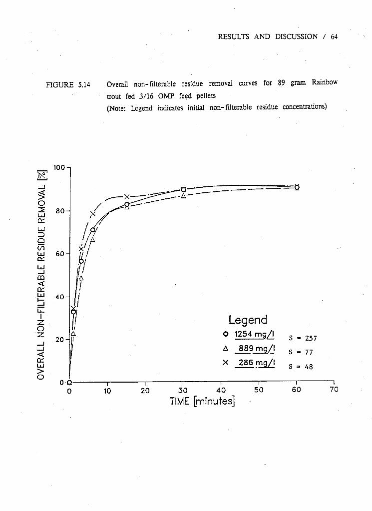
FIGURE 5.14 Overall non-filterable residue removal curves for 89 gram Rainbow-
trout fed .3/16 OMP feed pellets (Note: Legend indicates initial non-filterable residue concentrations)
100-i
80H
60 H
40 H
20 H
0 Q-0
Legend O 1254 mg/l A 889 mg/l X 286 mg/l
S = 257
S - 77
S - 48
10 20 40 30 TIME [minutes]
50 60 70

RESULTS AND DISCUSSION / 65
FIGURE 5.15 Overall non-filterable residue removal curves for 311 gram Rainbow trout fed 3/16 OMP feed pellets (Note: Legend indicates initial non-filterable residue concentrations)
TIME [minutes]

RESULTS AND DISCUSSION / 66
FIGURE 5.16 Individual particle settling velocity distribution curves for 11 gram Rainbow trout fed 3/32 OMP feed pellets (Note: Legend indicates initial non-filterable residue concentrations)
Legend O 651 mg/l s = 4 5
A 542 mg/l s = 78
1 2 3 4 PARTICLE SETTLING VELOCITY [cm/sec]

RESULTS AND DISCUSSION / 67
FIGURE 5.17 Individual particle settling velocity distribution curves for 17 gram . Rainbow trout fed 3/32 OMP feed pellets
(Note: Legend indicates initial non-filterable residue concentrations)
x i-i
< X to CO
o < Lu 0-j 1 1 1 1 1
0 1 2 3 4 5 PARTICLE SETTLING VELOCITY [cm/sec ]
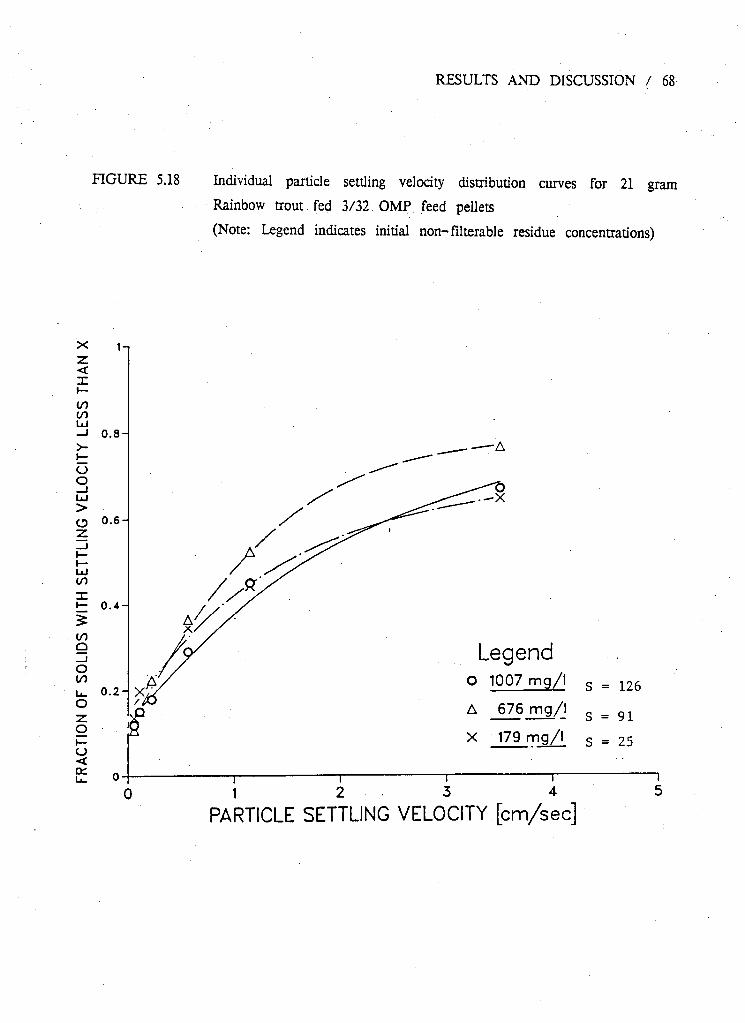
RESULTS AND DISCUSSION / 68
FIGURE 5.18 Individual particle settling velocity distribution curves for 21 gram Rainbow trout fed 3/32 OMP feed pellets
(Note: Legend indicates initial non-filterable residue concentrations)
z < X I— (/) to
o o _ J L U
>
to X
to Q _I o to
0.8-
0.6-
0.4-
L_ 0.2-O Z o o <
Legend O 1007 m g / l s
A 676 m g / l s
X 179 m g / l s
= 126
= 91
= 25
1~ 2 1 2 3 4
PARTICLE SETTLING VELOCITY [cm/sec]

RESULTS AND DISCUSSION / 69
FIGURE 5.19 Individual particle settling velocity distribution curves for 21 gram
Rainbow trout fed 1/8 OMP feed pellets
(Note: Legend indicates initial non-filterable residue concentrations)

RESULTS AND DISCUSSION / 70
FIGURE 5.20 Individual particle settling velocity distribution curves for 41 gram
Rainbow trout fed 1/8 OMP feed pellets
(Note: Legend indicates initial non-filterable residue concentrations)
Legend O 1755 m g / l s
A 1148 m g / l s
X 422 m g / l s
• 329 m g / l s
186
132
39
60
1 2 3 4
PARTICLE SETTLING VELOCITY [cm/sec]

RESULTS AND DISCUSSION / 71
FIGURE 5.21 Individual particle settling velocity distribution curves for 54 gram Rainbow trout fed 1/8 OMP feed pellets (Note: Legend indicates initial non-filterable residue concentrations)
x < X I— OO CO UJ - J 0.8->-
o _ l UJ > o 0.6-
u i OO
CO Q _ i o to
z o (— o <
0.4
0.2
Legend O 1945 m g / l
A 1308 m g / l
X 616 m g / l
i 4 1 2 3
PARTICLE SETTLING VELOCITY [cm/sec]
s
s
s
278
216
66
5

RESULTS AND DISCUSSION / 72
FIGURE 5.22 Individual particle settling velocity distribution curves for 54 gram Rainbow trout fed 5/32 OMP feed pellets (Note: Legend indicates initial non-filterable residue concentrations)
Legend O 7 9 2 m g / l
A 744- m g / l
X 595 m g / l
• 262 m g / l
s
s
s
s
13
126
120
83
"T" 4 1 2 3
PARTICLE SETTLING VELOCITY [cm/sec]
n 5

RESULTS AND DISCUSSION / 73
FIGURE 5.23 Individual particle settling velocity distribution curves for 73 gram
Rainbow trout fed 5/32 OMP feed pellets
(Note: Legend indicates initial non-filterable residue concentrations)

RESULTS AND DISCUSSION / 74
FIGURE 5.24 Individual particle settling velocity distribution curves for 93 gram Rainbow trout fed 5/32 OMP feed pellets (Note: Legend indicates initial non- filterable residue concentrations)
Legend O 594 mg/l A 503 mg/l X 397 mg/l • 332 mg/l
s
s
s
s
150
198
397
65
1 2 3 4 PARTICLE SETTLING VELOCITY [cm/sec ]

RESULTS AND DISCUSSION / 75
FIGURE 5.25 Individual particle settling velocity distribution curves for 89 gram Rainbow trout fed 3/16 OMP feed pellets (Note: Legend indicates initial non-filterable residue concentrations)
Legend O 1254 mg/l A 889 mg/l X 286 mg/l
4
S
s s
257
77
48
1 2 3
PARTICLE SETTLING VELOCITY [cm/sec]

RESULTS AND DISCUSSION / 76
FIGURE 5.26 Individual particle settling velocity distribution curves for 311 gram Rainbow trout fed 3/16 OMP feed pellets
(Note: Legend indicates initial non-filterable residue concentrations)

RESULTS AND DISCUSSION / 77
Comparison of the settling curves within a feed pellet size and between feed pellet
sizes should therefore identify any differences in the settling behavior of the wastes,
related to fish size and feed pellet size respectively. However, the form of the
non-filterable residue removal curve is not ideally suited to analysis. Statistical
procedures for handling complex non-linear functions are often complicated and more
difficult than for handling linear relationships. In some situations, however, it may be
possible to transform the x, and/or y variables in such a way that the resulting
function is close to being linear. A linear regression model can then be formulated in
terms of the transformed variables, and the appropriate analysis can be based on the
transformed data (Bhattacharyya & Johnson, 1977).
The data from the settling trials was therefore transformed in an effort to obtain an
approximate linear function. Two transformations were tested; LogX,Y and X.X/Y, a
linearization of the hyperbolic relationship
Y = ( AX ) / ( B + X ) (5.1)
Where Y percentage of non-filterable residue removed
X residence time (minutes)
A.B constants
Equation 5.1 is then linearized using the relationship
Z = b + b X o 1 (5.2)

RESULTS AND DISCUSSION / 78
Where Z X/Y (5.2.1)
b B/A (5.2.2) o
b. 1 1/A (5.2.3)
Both transformations produced linear regressions with high i2 (Sample Coefficient of
Determination) values, of 0.87 - 0.99 and 0.9996 - 1.0000 respectively. However, the
use of the LogX,Y transformation to fit the severe curve in the data is only valid at
short residence times. The relationship obtained in this transformation assumes that as
the residence time increases, so will the level of solids removal. Removal rates of
greater than 100% are thus possible at long residence times. This is clearly impossible.
However, in the hyperbolic relationship, as the residence time increases the
non-filterable residue removal curve increases to an asymptote or maximum level which
is less than 100%. This more accurately represents the situation occurring in the level
of removal of non-filterable residue as a function of time. The hyperbolic function
and it's linearized transformation was subsequently selected for this study.
It is important to note that in cases where the range in Y values is small, the r2
can be misleading. When Y is small, the transformation X/Y is similiar to dividing X
by a constant (k). When X/k is plotted as a function of X it will naturally produce
a perfect fit linear regression. Therefore the transformation should only be used when
the variation in Y values is large. Within the data obtained in the settling trials, the
level of removal (Y) varies from 24 - 93% during the 60 minute retention time (X).
This should be sufficiently large to permit the use of the X.X/Y transformation.
Appendix I summarizes the hyperbolic and the corresponding linear regression equations
for each of the overall non-filterable residue removal curves illustrated in Figures 5.5

RESULTS AND DISCUSSION / 79
- 5.15.
Differences in the overall non-filterable residue removal curves could now be identified
by comparing the linear regression equations for each X.X/Y transformed data group.
Regression equations may differ for two reasons; 1) they have different slopes, that is
they are not parallel , or 2) if. they are parallel, they may differ in level; that is
their intercepts are not equal . Two hypothesis that must be considered and tested are
therefore:
1) Slopes of linear functions are the same, slopes are parallel
2) Intercepts of linear functions are the same, intercepts are equal
One computer program suitable for performing these two tests is the Equality of Slope
Test program S:SLTEST. SLTEST is a self-contained program, available through the
public file S: SLTEST. A copy of the program description may be obtained through the
computing, center.
Simply, SLTEST computes the linear regression equation for each set of data and tests
whether the differences in the regression coefficients between groups are due to
sampling error, or may be attributed to differences between groups. The program uses
the F-test to check the hypothesis that each regression coefficient is identical among
all groups. Depending on the result of the F-test, the program will do one of two
things:
1) If the hypothesis is rejected, that is, the regression coefficients are different,
SLTEST will: a) find for each pair of equations the first regression coefficient in

RESULTS AND DISCUSSION / 80
which the above equations differ, or b) find, for each pair of equations, all the
regression coefficients in which the above equations differ.
2) If the hypothesis is not rejected, SLTEST will test the hypothesis that a common
equation can be used for all samples; that is, SLTEST will test if the intercepts with
the y-axis are equal.
SLTEST was subsequently used to test for similarities in the regression coefficients and
y-intercepts of the regression equations representing the overall non-filterable residue
removal curves.
As part of the experimental design, each waste group, identified by a weight class and
feed pellet size, was replicated. The replications of the settling trials were to be used
as a check for uniformity and reproducibility of the Type II settling curves. However,
due to the highly variable hydraulic conditions within the tank, the amount of
accumulated solids present after 24 hours was never constant The initial solids
concentration in each settling, trial was therefore different.
The degree of Type II or flocculant particle settling in a system, has been shown to
be a function of the suspended solids concentration, the particle size distribution, the
velocity gradient within the system, and the distance the particles are to settle.
Changing the initial solids concentration, while maintaining the latter three factors
constant, should therefore affect the level of Type II settling present and subsequently
the rate of solids removal. We may therefore expect some differences in the rates of
solids removal between replications with different initial solids concentrations.

RESULTS AND DISCUSSION / 81
Therefore, before comparisons could be made between waste groups it was first
necessary to determine if variations in the initial non-filterable residue concentrations
were significant The first hypothesis to be tested therefore was: 1) a single regression
equation can be used to represent the replicated settling curves in each group.
If the hypothesis is accepted, then the replicate curves in each group can be
represented by a single equation. The variation observed in the solids removal curves
within the group are therefore not significant Analysis of the groups is simplified
through the use of the single regression equation. However, if the hypothesis is
rejected, indicating that the variability observed in the inital non-filterable residue
concentrations is significant, then the analysis of the settling characteristics must also
include the effects of concentration. Further analysis between groups would have to
take initial solids concentration into consideration.
The linear regression equations summarized in Appendix I were subsequently compared
using. SLTEST at confidence levels of 0.05 and 0.01 (95% and. 99%),, to determine, if
the regression equations within each group could be pooled and represented by a
single, common regression equation.
Results of SLTEST at both confidence levels indicated that a common slope of 0.011
was present in all groups. However, common regression equations for each group were
not possible due to statistically significant variations in the y-intercepts (0.0116 -
0.0369).
A rejection of the hypothesis on this basis would appear to indicate that within the

RESULTS AND DISCUSSION / 82
range of initial concentrations observed in the settling trials (179 - 1945 mg/l), varying
the concentration did statistically affect the settling rate of the waste solids. This is
not surprising given the influence of concentration on the degree of flocculant settling
present in a suspension. At higher concentrations the opportunity for particle contact is
greater. Large, high velocity particulates can collide and coalesce with smaller less
settlable fractions, thereby facilitating their removal. The rate of removal of
non-filterable residue would subsequently be higher in the beginning, declining over
time as the concentration is reduced. A high correlation between the initial
concentration and the level of the y-intercept might therefore be expected. However,
when the y-intercepts and the initial concentrations ate compared within waste groups
and between groups (Figure 5.27), no correlation is evident (r2=0.077). Results of the
regression indicate approximately 8% of the variability in the y-intercepts is explained
by the concentration effect
The low correlation observed between the level of the y-intercept and the initial
concentration may be an indication that; 1) the range, of. concentrations observed in the
settling trials may be below the level at which Type II settling occurs, or 2) if Type
II settling is occurring at higher concentrations, it's contribution to the overall rate of
removal is insignificant. In either case it must be assumed that the variation observed
in the initial concentrations are not responsible for the variations in the y-intercepts.
In comparing the replications within each waste group, it has been assumed that, given
the feed pellet size and fish size were kept constant, wastes in each replication should
also be relatively uniform. However, it is impossible to control the amount of
fragmentation of faeces and unconsumed feed pellets resulting from repeated

RESULTS AND DISCUSSION / 83
FIGURE 5.27 Variability of the y-intercept of the linearized overall non-filterable residue removal curves as a function of the initial non-filterable residue concentration
oo1
ui .•> or r> o _J
o 3 UJ or Ul ZD a to
o or ui
0.5-.
0.4H
0.3H
CG < or ui
=1 0.2
o.H
0.0
OO Q o y
500 1000 1500 2000 2500 INITIAL NON-FILTERABLE RESIDUE REMOVAL CONCENTRATION [mg/i

RESULTS AND DISCUSSION / 84
resuspension and massication by fish. Some variation in the range of particle sizes
might therefore be expected. This could account for variations observed in the
y-intercepts. Wastes with a higher proportion of larger, faster settling particulates would
show a high level of removal within the early stages of settling, compared to a waste
with a lower proportion of the same size particles. However, the presence of a
common slope within the settling trials indicates there is a similarity in the settling
pattern of the waste solids. Given the assumption that the waste solids are behaving
as discrete entities, the proportional distribution of particle sizes and their respective
settling velocities should therefore be similar.
One method of determining the validity of this assumption is to test the regression
equations of the individual particle settling velocity distribution curves for a common
regression equation.
The individual particle settling velocity distribution curves were subsequently linearized
using the relationship in equations 5.1 - 5.2.3 and compared using SLTEST. Results of
SLTEST at a confidence level of 0.01 indicated that the pooled regressions can be
represented by a single, common equation (Equation 5.3).
Y - 92.59X/(2.01 + X) (5.3)
Where X = settfing velocity of particles (cm/sec)
Y = fraction of particles with settling velocities less than X
The proportional distribution of particle sizes within waste groups and between waste

RESULTS AND DISCUSSION / 85
groups must therefore be considered identical.
Analysis of the linearized overall non-filterable residue removal curves and the
subsequent determination of the source of the variations in the y-intercepts, has been
based on the premise that the difference in the y-intercepts is significant. It was
therefore concluded that the settling characteristics of the wastes must also be
significantly different However, the submission of a common regression equation,
characterizing the pooled linearized individual particle settling velocity distribution curves,
indicates that the proportional distribution of particle sizes within the wastes is
identical. It should therefore be assumed that if all extraneous factors such as
turbulence , short circuiting and upwelling within the column are kept constant, wastes
from different size fish or different size feed pellets should behave in a similar
manner. The variability observed within the y-intercepts must therefore be considered
the result of factors outside of those controlled in the settling trials.
Evaluation of the results of the SLTEST has also been based on the premise- that
given no common regression equation is possible due to statistically significant variations
in the y-intercepts, that these variations should be considered important when designing
a sedimentation basin. The variations observed in the settling behavior of the waste
solids might be considered significant, assuming a clarifier could be ideally designed
with no turbulence or short circuiting. However, given the nature of the design process
in which the settling curves are to be used, and the general inclusion of a large
safety factor (Warrer-Hansen, 1982), any differences observed between the settling
curves could be ignored for design purposes. It may therefore be assumed that within
the retention time (24 hours), fish sizes (llg-311g), feed type (OMP), and feed pellet

RESULTS AND DISCUSSION / 86
sizes (3/32-3/16) used, there is no significant difference in the settling behavior of the
waste solids produced.
A single curve can therefore be used to characterize the settling behavior of the waste
solids produced in the study. The individual non-filterable residue removal percentiles
and individual particle settling velocity distribution fractions were subsequently pooled in
order to produce the single overall non-filterable residue removal curve (Figure 5.28)
and the individual particle settling velocity distribution curve (Figure 5.29).
Analysis of Figure 5.28 shows that a residence time of 10-15 minutes is sufficient to
reduce the non-filterable residue by 82%. However, the curve also shows that holding
the effluent longer than 15 minutes, does not provide any appreciable increase in
solids removal. Increasing the residence time to 30 minutes, effectively doubling the
retention time, only increased the level of solids removal an additional 4 %. While
holding the effluent for 60 minutes produced a total increase of only 7%. Therefore,
selecting, a. retention, time greater than 15. minutes does not effectively increase the
level of solids removal. Selecting a retention time greater than 15 minutes also
increases, unnecessarily the size of the system, and consequently, the cost
ln a summary of capital, operating and maintenance costs as a function of surface
area (Figure 5.30), Underwood McLellan (1979) show that for small sedimentation
basins (<1000 m2), these three costs increase linearly with increasing surface area.
However, as the surface area of the sedimentation basin increases (>1000 m2), capital,
operating and maintenance costs begin to increase at a faster rate. It is therefore
desirable to select a residence time which minimizes the size of the treatment system,

RESULTS AND DISCUSSION / 87

RESULTS AND DISCUSSION / 88
FIGURE 5.29 Individual particle settling velocity distribution curve for Rainbow trout fed an Oregon Moist Pellet diet

RESULTS AND DISCUSSION / 89
FIGURE 5.30 Summary of capital, operating and maintenance costs for a sedimentation basin as a function of surface area (Underwood McLellan, 1979)
1,000,000
in or <
O 100,000,
in O o
10,000.
1,000 Jt .3 .4 .5 .6 .7 J J I 2 3 4 3 6 7 8 9|0 2 3 4 3 6 7 * »100
SURFACE AREA ( m 2 x 100)

RESULTS AND DISCUSSION / 90
while still achieving the desired level of solids removal.
Holding the effluent in contact with the settled solids for long periods is also
undesirable as decomposition and leaching of the organic solids reduces the level of
dissolved oxygen (02) and increases the level of dissolved nutrients in the clarified
effluent
Figure 5.28, illustrating the distribution of individual particle settling velocities within
the waste solids, shows the solids particulates settled at significantly higher rates than
reported by Walden & Birkbeck (1977) or Stechey (1986). Walden & Birkbeck (1977)
report that the waste solids exhibited two main settling fractions. Over 50% of the
solids settled faster than 0.2 cm/sec, while 40% had settling rates faster than 0.51
cm/sec. Using these velocities for comparison, the waste solids generated from feeding
the Oregon Moist Pellet ® feed, showed over 80% of the solids had settling rates
faster than 0.2 cm/sec, while 72% had settling rates faster than 0.51 cm/sec.
The purpose of this study was; 1) to characterize the settling behavior of waste solids
from a trout culture unit as a function of fish size and feed pellet size, and 2) relate
the results to current gravity solids separation system design proceedures.
Using the overall non-filterable residue removal curves, and individual particle settling
velocity distribution curves, it was possible to show that solid wastes retained for 24
hours exhibited uniform settling behavior. Differences in settling rates of fresh excreta,
reported as a function of fish size (Wheaton, 1977; Warrer-Hansen, 1979) or pellet
size (Walden & Birkbeck, 1974) were negated by physical and chemical processes

occurring in the holding tank.
RESULTS AND DISCUSSION / 91
The curves produced in this study provide the basis for the selection of a suitable
retention time and depth for a gravity solids separation system to treat the cleaning
flows from a fish farm or hatchery employing a 24 hour cleaning cycle.
Appendix II summarizes the use of the overall non-filterable residue removal curve
and individual particle settling velocity distribution curve for sizing a gravity solids
separation system for a fish farm producing 50-75 tonnes of fish a year, utilizing
approximately 500 liters of water per second.

6. CONCLUSION
The findings of this study can be summarized as follows: Flocculant particle or Type
II settling curves were used to derive the overall non-filterable residue removal and
individual particle settling velocity distribution curves for Rainbow Trout {Salmo
gairdneri) culture cleaning wastes. Analysis of the curves using the Equality of Slope
Test (S:SLTEST), showed that there was no significant difference in the settling
behavior of the particulate solids when wastes from different size fish or different size
feed pellets were compared. A single curve was therefore used to characterize each of
the non-filterable residue removal curves (Figure 5.28) and individual particle settling
velocity distribution curves (figure 5.29) derived in the study.
The overall non-filterable residue removal curve showed that the bulk of the waste
solids removal (>80%) occurs within the first 15 minutes of settling. Holding the
waste longer than 15 minutes did not contribute significantly to the overall level of
solids removal.
The individual particle settling velocity distribution curve showed the solids produced in
the study using the Oregon Moist Pellet ® feed settled at a faster rate than reported
in the literature for non-fresh excreta, but slower than for fresh excreta.
Differences due to fish size and feed pellet size in the settling behavior of the waste
solids, reported in the literature, were not apparent when the waste solids were
retained within the culture tank for 24 hours.
92

7. RECOMMENDATIONS FOR FUTURE WORK
7.1. RESIDENCE TIME
Muir (1978) and Warrer-Hansen (1979;1982) have shown that the length of time the
waste solids are retained within the culture unit can significantly reduce the settleability
of those solids. In our study, we selected a retention time of 24 hours as being fairly
representative of the length of time waste solids would be retained in a commercial
fish farm or government hatchery employing a daily cleaning schedule of the ponds or
raceways. The overall solids removal and individual particle settling velocity distributions
were subsequently higher than generally reported in the literature where longer
retention times are involved. One area for further work would therefore be to quantify
the effects of retention time on the settleability of waste solids. The results to be
used as a management tool in scheduling tank cleaning intervals for optimum solids
removal efficiency within the gravity solids separation system.
A. further, area of research, associated with residence time, is the amount of physical
shearing, hydration and resuspension of the waste solids within the culture units. These
parameters all act to reduce the particle size and density of the waste solids. However,
the magnitude of these processes will be a function of the flow rate, hydraulic
characteristics of the tank and the stocking density, all of which are site specific.
The waste solids collected in our study were subjected to physical agitation and
resuspension as a result of the high stocking densities used in the small 200 litre
tanks. However, it is difficult to judge if these conditions would be comparable to
those found in the larger production units. In some raceways and circular ponds, dead
93

RECOMMENDATIONS FOR FUTURE WORK / 94
zones provide a collection point for waste solids, which may then undergo little
physical shearing. While some solids may be subjected to extreme physical agitation as
the effluent cascades from one raceway to another, or is circulated by a mechanical
aeration unit Given that these are all site specific factors, one recommendation is to
compile a series of settling curves for a variety of farms and hatcheries, to determine
if the waste solids can be characterized by the holding system used (eg. raceway,
Burrows pond, circular pond etc.).
7.2. FEED T Y P E
This research has shown that the waste solids produced from Rainbow trout fed the
Oregon Moist Pellet ® diet, settle at a higher rate than reported in the literature for
dry pellet feeds (Walden & Birkbeck, 1974; Stechey, 1986).
An attempt was made to compare the OMP feed with a dry pellet feed (Purina Trout
Chow ®). However, the hydraulic conditions within the holding tank units used, were
not suitable and. very little waste solids were retained. It is therefore recommended
that a different holding tank be used which will retain the solid wastes, or use
cleaning wastes from farms or hatcheries using the dry feed, in the settling trials.
Similiar settling trials could also be carried out on other pellet feeds such as EWOS
®, Rangen ®, and BIO-Dyne ®. Other feed types which might be investigated are
trash fish, and the wet feeds which are produced on site at the farms, now being
used extensively in the salmon farming industry.

REFERENCES Bergheim, A. & A.R.,Selmer-01sen 1978. "River Pollution from a Large Trout Farm in
Norway". Aquaculture (14):267-270
Bergheim, A. & A.,Silversten 1981. "Oxygen Consuming Properties of Effluents from Fish Farms". Aquaculture (22): 185-187
Bergheim, A.,H.,Hustveit, A.,Kittelsen, & A.R.,Selmer-01sen 1984. "Estimated Pollution Loadings from Norwegian Fish Farms II: Investigations 1980-81". Aquaculture (36): 157-168
Bhattacharyya, G.K., & R.A., Johnson 1977. "Statistical Concepts and Methods". Wiley Series in Probability and Mathematical Statistics., John Wiley & Sons, New York.
Bodien, D.G. 1970. "An Evaluation of Salmonid Hatchery Wastes". U.S. Dept Inter. Fed. Water Qual. Adm. Portland, Oregon PB 215496, 53pp.
Brisbin, K.J. 1970. "Report on the Pollutional Aspects of Trout Hatcheries in British Columbia". Prepared for Fish and Wildlife Branch, Dept. Recreation Cons., Underwood McLellan & Associates.
Brockway, D.R. 1950. "Metabolic Products and Their Effects". Prog. Fish-Cult 12(3): 127-129.
Brown, CM. & C.E.,Nash 1979. "Aquaculture as a Method for Meeting Hatchery Discharge Standards". Presented at Bio-Engineering Symposium, Traverse City, Michigan. October, 1979.
Butz, I. & B.,Vens-Cappell 1982. "Organic Load from the Metabolic Products of Rainbow Trout Fed with Dry Food". In: Report of the EIFAC Workshop on Fish-Farm Effluents. Silkeborg, Denmark 26-28 May, 1981. EIFAC Technical Paper (41).
Chesness, J.L., L.J.,Fussel & T.K.,Hill 1973. "Mechanical Efficiency of a Nozzel Aerator". Transactions of the ASAE 16(1):67-8,71.
95

/ 96
Chesness, J.L, W.H.,Poole & T.K.,Hill 1975. "Settling Basin Design for Raceway Fish Production Systems". Transactions of the ASAE:Paper No. 74-5005. pp326-331.
Clark, J.W., V.,Warren & M.J.,Hammer 1977. "Water Supply and Pollution Control". Third Edition. Harper & Row, New York, pp 351-359.
DFO, unpublished. Department of Fisheries and Oceans internal survey of Federal hatcheries. Environmental assessment of down stream effects of hatchery effluents (1978-1981).
EIFAC (European Inland Fisheries Advisory Council), 1982. "Report of the EIFAC Workshop on Fish-Farm Effluents". Silkeborg, Denmark 26-28 May, 1981. EIFAC Technical Paper (41).
Faure, A. 1977. "Mise au point sur la pollution engendreE les pisciculture". Piscic.Fr.(50):33-35.In: Report of the EIFAC Workshop on Fish-Farm Effluents. Silkeborg, Denmark 26-28 May, 1981. EIFAC Technical Paper (41).
Gunther, D.C.,D.E.,Brune & G.A.E.,Gall 1981. "Ammonia Production and Removal in a Trout Rearing Facility". Transactions of the ASAE. ppl376-1380,1385.
Huber, R.T. & J.J.,Valentine 1978. "Analysis and treatment of Fish Hatchery Effluents". Report from Lamar National Fish Hatchery Development Center, Lamar Pennsylvania.
Hydroscience Inc.1977. In: Underwood McLellan, 1979. "Salmon Rearing Facilities,Waste Water Study, Treatment Technology". Underwood McLellan (1977) Ltd., Consulting Engineers and Planners, Vancouver, B.C.
Klontz, G.W. & J.G.,King 1975. "Aquaculture in Idaho and Nation Wide". Idaho Dept. of Water Resources Research Technical Completion report. IDWR Project 45-080, 86pp.
Klontz, G.W.,I.R.,Brock & J.A.,MacNair 1978. "Aquaculture Techniques Water Use and
Discharge Quality". Moscow, Idaho. University of Idaho, Office of

/ 97
Water Research and Technology. Project A.054-1DA, 88pp.
Knbsche, R. & E.Tscheu 1974. "Some Initial Aquaculture Experiments in Recirculating Water Systems". Aquaculture (ll):323-328.
Liao, P.B. 1970. "Pollution Potential of Salmonid Fish Hatcheries". Water Sewage Works 117(8):291-7.
Liao, P.B. 1970a. "Salmonid Hatchery Wastewater Treatment". Water Sewage Works 117(2):434-43.
Liao, P.B. 1971. "Water Requirements of Salmonids". Prog.Fish-Cult 33:210-15.
Liao, P.B. & R.,Mayo 1972. "Salmonid Hatchery Water Reuse systems". Aquaculture (l):317-335.
Liao, P.B. & R.,Mayo 1974. "Intensified Fish Culture Combining Water Reconditioning with Pollution Abatement". Aquaculture (3):61—85.
Liao, P.B., R.D.,Mayo & W.,Williams 1972. "A Study for Development of Fish Hatchery Water Treatment System". Report Prepared for the Walla Walla District Corps, of Engineers. Kramer, Chin & Mayo, Consulting Engineers; Seattle, Washington.
Mantle, G.J. 1982. "Biological and Chemical Changes Associated With the Discharge of Fish Farm Effluents". In: Report of the EIFAC Workshop on Fish-Farm Effluents. Silkeborg, Denmark 26-28 May, 1981. EIFAC Technical Paper (41).
Mayo, R.D. & P.B.,Liao 1969. "A Study of the Pollutional Effects of Salmonid Hatcheries". A Report Prepared for the States of Wisconsin, New York and Michigan., Kramer, Chin & Mayo, Consulting Engineers, Seattle, Washington.
Muir, J.F. 1978. "Aspects of Water Treatment and Reuse in Intensified Fish Culture". Ph.D. Thesis. Glasgow, Scotland. University of Strathclyde, 451pp.

/ 98
Muir, J.F. 1982. "Economic Aspects of Waste Treatment in Fish Culture". In: Report of the EIFAC Workshop on Fish-Farm Effluents. Silkeborg, Denmark 26-28 May, 1981. EIFAC Technical Paper (41).
Muir, J.F. & R.I.,Lipper 1970. From: Muir, J.F. 1982. "Economic Aspects of Waste Treatment in Fish Culture".
Parker, N.C. & M.C.,Broussard 1977. "A Selected Bibliography of Water Reuse Systems for Aquaculture". Texas Agric. Exp. StaL 33pp.
Petit, J. 1978. "Treatment Experiments of the Water Discharged by a Fish Farm". Technical Report of the Mission in UK. Jony en Josas, INR A, 30pp.
Querellou, J.,A.,Faure & C.,Faure 1982. "Pollution Loads from Rainbow Trout Farms in Brittany, France". In: Report of the EIFAC Workshop on Fish-Farm Effluents. Silkeborg, Denmark 26-28 May, 1981. EIFAC Technical Paper (41).
Samis, S. 1983 Personal Communication.
Scherb, K. & F.,Braun 1971. "Erfahrungen mit der Intensivhaltung von Regenbogenforellen bei biologischer Reinigung des Abwassers mit belebten Schlamm im Kreislaufsystem, Wasser-Abwasser-Forsch".(4):118-24 In: Report of the EIFAC Workshop on Fish-Farm Effluents. Silkeborg, Denmark 26-28 May, 1981. EIFAC Technical Paper (41).
Solbe, J.F. de L.G. 1982. "Fish Farm Effluents: A United Kingdom Survey". In: Report of the EIFAC Workshop on Fish-Farm Effluents. Silkeborg, Denmark 26-28 May, 1981. EIFAC Technical Paper (41).
Solberg, S. & F.,Bregnballe 1977. "Dambrug som forurenigskilde". Medd. ForsogsdambrugeL (58) In: Report of the EIFAC Workshop on Fish-Farm Effluents. Silkeborg, Denmark 26-28 May, 1981. EIFAC Technical Paper (41).
Solberg, SO. & F.,Bregnballe 1982. "Pollution from Farmed Trout Fed with Minced

/ 99
Trash Fish". In: Report of the EIFAC Workshop on Fish-Farm Effluents. Silkeborg, Denmark 26-28 May, 1981. EIFAC Technical Paper (41).
Sparrow, R.A.H. 1981. '"Hatchery Effluent Water Quality in B.C.". In:Bio-Engineering Symposium for fish culture. FCS Publ. 1:162-166.
Speece, R.C. 1973. "Trout Metabolism Characteristics and the Rational Design of Nitrification Facilities for Water Reuse in Hatcheries". Trans. Am. Fish. Soc. 102:323-334.
Stechey, D. 1986. Personal Communication
Sumari, O. 1982. "A Report on Fish-Farm Effluents in Finland". In: Report of the EIFAC Workshop on Fish-Farm Effluents. Silkeborg, Denmark 26-28 May, 1981. EIFAC Technical Paper (41).
Tchobanoglous, G. 1979. "Wastewater Engineering: Treatment,Disposal,Reuse". Second Edition. Metcalf & Eddy, Inc. McGraw Hill Book Company.
Underwood McLellan & Associates Ltd 1970. "Report on Pollutional Aspects of Trout Hatcheries in B.C.". Prepared for: Department of Recreation and Conservation. Fish and Wildlife Branch
Underwood McLellan & Associates 1977. ImUnderwood McLellan & Associates 1979. "Salmon Rearing Facilities, Water Study, Treatment Technology". March 1979. Underwood McLellan (1977) Ltd., Consulting Engineers and Planners, Vancouver, B.C.
Underwood McLellan & Associates 1979. "Salmon Rearing Facilities, Waste Water Study, Treatment Technology". March, 1979. Underwood McLellan (1977)Ltd., Consulting Engineers and Planners, Vancouver,B.C.
Walden, CC. & A.E.,Birkbeck 1974. "Feasibility and Design Studies for Water Treatment at a Trout Hatchery". Prepared for British Columbia Department of Public Works by B.C. Research, Vancouver, 234pp.

/ 100
Warrer-Hansen, I. 1979. "Fish Farming and Pollution Problems-Methods to Reduce Discharged Matter". Paper Presented at the Fish Farming Meeting, Oban, 22-23 February, 1979.
Warrer-Hansen, I. 1979a. "Operation Clean-Up". Fish Farming Int 6(2):32-34.
Warrer-Hansen, I. 1982. "Methods of Treatment of Waste Water from Trout Fanning". In: Report of the EIFAC Workshop on Fish-Farm Effluents. Silkeborg, Denmark 26-28 May, 1981. EIFAC Technical Paper (41).
Wheaton, F. 1977. "Aquaculture Engineering". John Wiley & Sons. Inc.
Willoughby, H., H.N.,Larsen & J.T. Bowen 1972. "The Pollutional Effects of Fish Hatcheries". American Fishses & U.S. Trout News. 17(3): pp6-7,20-1.

APPENDIX I
TABLE V SLTEST generated regression equations for overall non-filterable residue removal curves (Figures 5.5 - 5.15)
Group 9 Fish Feed P e l l e t Non-Filcerable Linear Hyperbolic Size Size (inch) Residue (cone) Trans formation Equati L on
1 11.0 3/32 65 I Y-0 .036 + 0.011X Y-89,3X/ [3. 19+X) 542 Y-0.026 + 0 .01IX Y-89 .6X/( 2.35+X)
2 17.0 3/32 738 Y-0 .037 + 0.01 IX Y-92 .7X/( 3.41+X) 584 Y-0.026 + 0.011X Y-90.8X/< [2.33+X) 402 Y-0.022 + 0 .011X Y-88.8X/< kl.95+X)
3 21.0 3/32 1007 Y-0.020 + 0.011X Y-90.7X/ [1.78+X) 676 Y-0.032 + 0.011X Y-93.6X/ [2.9 8+X) 179 Y-0.023 + 0 .011X Y-88.6X/ [2.03+X)
4 21.0 1/8 903 Y-0.022 + 0.011X Y-88.3X/ [1.9 3+X) 794 Y-0.027 + 0 .011X Y-93.5X/ [2.49+X) 584 Y-0.026 + 0 .011X Y-94.6X/ [2.45+X)
5 41.0 1/8 1755 Y-0.021 + 0 .011X Y-95.IX/ [2.03+X) 1148 Y-0.021 + 0.011X Y-93.7X/ [1.9 4+X) 422 Y-0.020 + 0.011X Y-94.3X/ [1.91+X) 329 Y-0.012 + 0.011X Y-90.9X/ (1.06+X)
6 54.0 1/8 1945 Y-0.031 0.011X Y-92.9X/ (2.92+X) 1308 Y-0.025 + 0.011X Y-95 .OX/ (2.4 +X) 616 Y-0.017 + 0.011X Y-96.2X/ (1.67+X)
* Fi s h s i z e i n grams ** I n i t i a l n o n - f i l t e r a b l e residue concentration i n mg/litre
X = Residence time (minutes) Y = N o n - f i 1 t e r a b l e residue removed at res i d e n c e time X (%)
101

I 102
TABLE V ( c o n t . ) SLTEST generated regression equations for overall
non-filterable residue removal curves (Figures 5.5 - 5.15)
Group it Fish Feed P e l l e t Non-Filterable Linear Hyperbolic Size Size (inch) Residue (cone) Transformation Equation
7 54.0 5/32 792 Y = 0 .016 + 0 .011X Y=94.2X/(1 .53+X) 744 Y=0 .014 + 0 .01IX Y=93.6X/(1 .30+X) 595 Y=0.021 + 0.011X Y=91.7X/(1 .96+X) 262 Y = 0 .012 + 0 .011X Y=9 3.2X/(1 .14+X)
8 73.0 5/32 792 Y = 0 .017 + 0 .011X Y=94.9X/(1 •62+X) 693 Y=0.017 + 0 .011X Y=95 .9X/(1 .67+X) 657 Y=0.014 + 0 .011X Y=93.0X/(1 .34+X) 543 Y=»0.021 + 0.011X Y=91.4X/(1 .96+X)
9 93.0 5/32 594 Y=0 .016 + 0 .011X Y-92 .9X/(1 .46+X) 503 Y=0.022 + 0 .011X Y=94.3X/(2 .07+X) 397 Y=0.019 + 0 .011X Y=94.0X/(1 .75+X) 332 Y=0 .022 + 0.011X Y=91.2X/(2 .0 3+X)
10 89.0 3/16 1254 Y = 0 .020 + 0 .01IX Y=94.1X/(1 .87+X) 889 Y=»0.02 9 + 0.011X Y=94.9X/(2 .75+X) 286 Y-0 .015 + 0.011X Y-93.9X/(1 .43+X)
11 311.0 3/16 977 Y=0.020 + 0 .011X Y=94.8X/(1 .91+X)
* F i s h s i z e i n grams ** I n i t i a l n o n - f i l t e r a b l e residue concentration i n mg / l i t r e
X = R e s i d e n c e time ( m i n u t e s ) Y = N o n - f i 1 t e r a b l e r e s i d u e removed a t r e s i d e n c e t i m e X (%)

APPENDIX II
Figures 5.28 (overall non-filterable residue removal curve) and 5.29 (individual particle
settling velocity distribution curve) can be used to estimate the overflow rate
(mVmVhour) and residence time for various per cent solids removal.
In the example to be discussed, a fish farm producing 50-75 tonnes per year uses an
estimated 500 1/sec or 1800 mVhour. From the observations and discussions of the
overall non-filterable residue removal curve (Figure 5.28) it was concluded that holding
the effluent longer than 15 minutes did not effectively contribute to the overall level
of solids removal. Therefore, assuming a maximum residence time of 15 minutes will
provide for 82% removal of the non-filterable solids.
An overflow rate or surface loading rate can thus be obtained by selecting a suitable
settling velocity (V ) from the individual particle settling velocity distribution curve o
(Figure 5.29) such that 82% of the solid particulates will be removed. From Figure
5.29 it can be. observed, that 82% of the particles have settling, velocities greater than
0.2 cm/sec (7.2 m/hour).
From the discussion of Equations 3.1 and 3.2 it was shown that the settling velocity
is the equivalent of the overflow rate or surface loading rate. A settling velocity of
7.2 m/hour is therefore the equivalent of a loading rate of 7.2 mVmVhour.
Introducing a safety factor of 1.5 to reduce turbulence (Warrer-Hansen, 1982), yields a
surface loading rate of 5 m3/mVhour.
Given the water consumption of the farm is 1800 mVhour, the necessary basin area
103

/ 104
will be:
Sur face area of c l a r i f i e r
Flow rate Overflow rate
1800 m / h o u r
3 2 5 m /m / h o u r '= 360 m
Therefore, a farm utilizing 1800 mVhour, requiring 82% of non-filterable solids
removal, will require a sedimentation basin with a depth of 1.25 .m and a surface
area of 360 mJ. A width of 10-20 meters will maintain the water velocity in the
settling zone within the 2-4 an/sec maximum velocity suggested to prevent scouring
and resuspension of the already settled solids (Warrer-Hansen, 1982).