Embed Size (px)
Citation preview

i
DETERMINATION OF SELECTED HEAVY METALS POLLUTANTS AND
PHYSIO-CHEMICAL PARAMETERS IN SEDIMENTS AND WATER: A CASE
STUDY OF RIVER ATHI MACHAKOS COUNTY
By
JOHNSTONE KOSGEY
B.Ed.
THIS THESIS IS SUBMITTED IN PARTIAL FULFILLMENT OF THE
REQUIREMENTS FOR THE AWARD OF DEGREE OF MASTER OF SCIENCE
IN ANALYTICAL CHEMISTRY, UNIVERSITY OF ELDORET, KENYA.
NOVEMBER, 2013
ii
DECLARATION
Declaration by the student
This thesis report is my own original work and has not been presented for a degree in any
other University. No part of this thesis may be reproduced without the prior knowledge of
the author and/or university of Eldoret.
JOHNSTONE KOSGEY - SC/PGC/007/10
Signature……………………………….. Date………………………….
Declaration by the university supervisors
This thesis has been submitted for examination with our approval as University
supervisors.
DR.Y. MITEI CHERUIYOT
Department of Chemistry and Biochemistry
University of Eldoret
P.O. Box 1125
ELDORET
Signature …………………………… Date ……………………………
Prof. F. SEGOR
Department of Chemistry and Biochemistry
University of eldoret
P.O. Box 1125
ELDORET

iii
Signature …………………………… Date …………………………
ACKNOWLEDGEMENT
I express my sincere gratitude to Dr. J. Cheruiyot and Prof. F. Segor for their time,
straight talk and guiding comments. I owe much thanks to the Chemistry and
Biochemistry Department, university of Eldoret College for their technical support.
Finally, appreciation goes to all my family, colleagues and friends for the support and
encouragement they always gave me.
iv
ABSTRACT
The study set out to evaluate the effect of industrial activities by analyzing selected heavy
metals and physicochemical parameters of water. Chemical survey was conducted in 9
selected sites (potential polluting sites) along Athi river to determine the levels of heavy
chemical elements; lead (Pb), Copper (Cu), chromium (Cr), Nickel(Ni) Cadmium(Cd)
and to asses water quality based on physicochemical parameters. The variation in
concentration of these metals in the water and sediments as well as other water quality
parameters was a key factor to establish the pollution levels in different parts of the river.
The recommended WHO procedures of water sampling and analyses were followed.
Atomic absorption spectrometry analytical technique was used in the determination of the
heavy metal levels dissolved in the water and sediments samples. The results obtained in
water samples ranged from Pb( 0.23-0.54mg/L),Cu(0.0082-0.0163mg/L), Ni(0.0081-
0.0284mg/L), Cr(0.1363-0.3255mg/L), Cd(0.0117-0.0240mg/L) and for sediment
samples Pb(0.1277-0.3513mg/L), Cu(0.0607-0.1386mg/L),Ni(0.0191-0.0498mg/L),
Cr(0.0692-0.1329mg/L) and Cd(0.0108-0.0428mg/L). The values recorded for
physicochemical parameters were pH(6.5-7.4), TDS(109-136mg/L), COD(66-102mg/L),
BOD(6-15mg/L) and conductivity(155-206 µs/cm). From the results it was evident that
the water was heavily polluted and not fit for domestic, agricultural and industrial
purposes. Four of the analyzed heavy metals Pb, Cr, Cd and Ni surpassed the
recommended WHO maximum permissible limits (0.01mg/L), (0.01mg/L), (0.003mg/L)
and (0.001mg/L) respectively. Lead and chromium had the highest levelss in both
sediments and water while Cd and Ni had the lowest concentrations. A Kruskal-Wallis
test which, was conducted for the mean heavy metal concentrations, BOD, pH,
Conductivity, TDS and COD to determine the significant difference of these water
quality parameters in the nine different sampling locations showed significant
differences between heavy metals in water and sediments and heavy metals in different
stations(p<0.05). ANOVA test on pH did not reveal any significant difference (p<0.05)
between the means of the various locations sampled and all results obtained fell within
national and international standards of ESEPA/WHO. The BOD values were all higher
than the normal BOD for unpolluted water of ≤ 2mg/L. The variation of electrical
conductivity and TDS gradually decreased downstream with a slightly sharp rise at the
middle of the sampling points; with observed TDS levels falling below the EPA's
recommended maximum of TDS(500mg/L) in water. The COD values obtained were
weak < 400mg/L.However, comparing all the observed values with the EPA regulations,
the waters of this river is unsafe for domestic, industrial or agricultural use.
v
TABLE OF CONTENTS
DECLARATION ..............................................................................................................i
ACKNOWLEDGEMENT ............................................................................................. iii
ABSTRACT ................................................................................................................... iv
TABLE OF CONTENTS ................................................................................................. v
CHAPTER ONE ............................................................................................................ 1
INTRODUCTION ......................................................................................................... 1
1.1 General introduction ............................................................................................. 1
1.3 Justification......................................................................................................... 4s
1.4 Objectives ............................................................................................................. 6
1.4.1 General objective ............................................................................................... 6
1.4.2 Specific objectives ............................................................................................. 6
1.4.3 Hypothesis ............................................................................................................ s
CHAPTER TWO ........................................................................................................... 8
LITERATURE REVIEW.............................................................................................. 8
2.1 Review of related work done ................................................................................. 8
2.2 Specific heavy metal sources ........................................................................... 10
2.2.1 Cadmium .................................................................................................. 10
2.2.2 Copper ..................................................................................................... 11
2.2.3 Lead ......................................................................................................... 12
2.2.4 Chromium ................................................................................................ 12
2.2.5 Nickel ......................................................................................................... 13
2.3 Health effects of heavy metals ......................................................................... 14
vi
2.4 Bioaccumulation of heavy metals .................................................................... 17
2.5 Oxygen Demand .............................................................................................. 19
2.5.1 Biochemical Oxygen Demand (BOD) ............................................................ 19
2.5.2 Chemical Oxygen Demand(COD) ............................................................ 21
2.6 Total dissolved solids ........................................................................................... 22
2.7 Electrical conductivity .......................................................................................... 25
2.8 pH (potential of hydrogen) .................................................................................. 27
2.9 Methods of heavy metals analysis .................................................................... 28
2.9.1 Inductively Coupled Plasma Mass Spectrometry ...................................... 29
2.9.2 Atomic Emission Spectroscopy (AES) ..................................................... 29
2.9.3 Atomic Fluorescence Spectroscopy (AFS) ................................................ 30
2.9.4 Atomic Absorption spectroscopy (AAS) ................................................... 30
CHAPTER THREE ..................................................................................................... 35
MATERIALS AND METHODS ................................................................................. 35
3.1 Study area ............................................................................................................ 35
3.2 Chemicals and reagents ........................................................................................ 38
3.4Sampling ............................................................................................................... 39
3.5 Sample collection ................................................................................................. 39
3.6 Preparation of standards ....................................................................................... 40
3.7 Sample preparation and experimental procedures ............................................ 40
3.7.1 Sediment samples for heavy metal determination ........................................... 40
3.7.2 Water samples for heavy metal determination ............................................... 41
3.7.5 Analysis of pH .............................................................................................. 44

vii
3.7.6 Electrical conductivity .................................................................................. 45
CHAPTER FOUR ....................................................................................................... 47
RESULTS AND DISCUSSION ................................................................................... 47
4.1 Heavy metal analysis ....................................................................................... 47
4.1.1 Calibration Curves for Heavy metals ........................................................ 47
4.1.2 Heavy Metals distribution on flowing river water. .................................... 47
4.1.3 Heavy metals in sediments ................................................................................ 54
4.1.4 Physicochemical parameters .............................................................................. 63
CHAPTER FIVE ......................................................................................................... 70
CONCLUSION AND RECOMMENDATIONS ........................................................ 70
5.0 Conclusion ...................................................................................................... 70
5.2 Recommendations ........................................................................................... 71
REFERENCES ............................................................................................................ 72
APPENDICES ............................................................................................................. 83

viii
LIST OF APPENDICES
Appendix 1: Cu calibration curve .................................................................................. 83
Appendix 2: Cd calibration curve .................................................................................. 84
Appendix 3: Cr calibration curve ................................................................................... 85
Appendix 4: Ni calibration curve ................................................................................... 86
Appendix 5: Pb calibration curve ................................................................................... 87
Appendix 6: Cd absorbance peak ................................................................................... 88
Appendix 7: Cr absorbance peak.................................................................................... 89
Appendix 8: Cu absorbance peak ................................................................................... 90
Appendix 9: Pb absorbance peak ................................................................................... 91
Appendix 10: Ni absorbance peak .................................................................................. 92
Appendix 11: EPA maximum limits for different heavy metals ...................................... 93
Appendix 12: WHO, FAO and KEBS maximum limits for different heavy metals ......... 94
Appendix 13: EPA regulations on TDS.......................................................................... 95
Appendix 14: EPA classification of water COD ............................................................. 96

ix
LIST OF FIGURES
Figure 3. 1: Map of the study area .................................................................................. 37
Figure 4. 1: Variation of Copper concentrations in in water in mg/L .............................. 48
Figure 4. 2: Variation of lead concentrations in water in mg/L ....................................... 50
Figure 4. 3: Variation of Chromium concentrations in water in mg/L. ............................ 51
Figure 4. 4: Variation of Cadmium concentrations in water in mg/L. ............................. 52
Figure 4. 5: Variation of Nickel concentrations in water in mg/L. .................................. 52
Figure 4. 6: The variation of all the tested heavy metals on river water in mg/L ............. 54
Figure 4. 7: Variation of Copper concentrations in sediments in mg/L along Athi River 55
Figure 4. 8: Variation of Lead concentrations in sediments in mg/L along Athi River .... 56
Figure 4. 9: Variation of Cadmium concentrations in sediments in mg/L along Athi River57
Figure 4. 10: Variation of Chromium concentrations in sediments in mg/L ................... 58
Figure 4. 11: : Variation of Nickel concentrations in sediment in mg/L .......................... 59
Figure 4. 12: Comparative line graph showing the variation of all the tested heavy metals
on sediments in mg/L along the river ...................................................................... 60
Figure 4. 13: Bar-graph showing the comparative concentrations between water and
sediments in mg/L for the 5 heavy metals in the 9 sample stations from station 1to
station 9 .................................................................................................................. 61
Figure 4. 14: Variation of pH along the river ................................................................. 63
Figure 4. 15: Variation of BOD along the river in mg/L ................................................. 65
Figure 4. 16: Variation of conductivity along the river in μS/cm .................................... 66
Figure 4. 17: Variation of TDS along the river mg/L...................................................... 67
Figure 4. 18: Variation of COD along the river mg/L ..................................................... 68
x
Figure 4. 19: Comparison between BOD and COD in mg/L ........................................... 68
LIST OF TABLES
Table 4. 1: The Mean Variation of heavy metal concentrations in mg/L on river water
downstream ............................................................................................................ 53
Table 4. 2: Mean Variation of Heavy metal concentrations in sediments in mg/L
downstream ............................................................................................................ 61
xi
LIST OF ACRONYMS
AAS Atomic Absorption Spectroscopy
AES Atomic Emission Spectroscopy
AFS Atomic Fluorescent Spectroscopy
ANOVA Analysis of variance
ARBP Athi River Basin Program
BOD Biological oxygen demand
CBOD Carbonaceous biochemical oxygen demand
COD Chemical oxygen demand
CNS Central nervous system
DO Dissolved oxygen
EPA Environmental protection agency
FAO Food and Agriculture Organization.
Fig Figure
HNO3 Nitric acid
HCl Hydrochloric acid
IC Inorganic carbon
ICPMS Inductively Coupled Plasma Mass Spectrometry
ICPOES Inductively coupled plasma optical emission spectroscopy.
KEBS Kenya bureau of standards
km2
Kilometer squared
L litre
mg/L Milligram per litre
NEMA National environmental management authority
OD oxygen demand
pH Potential of hydrogen
PNS peripheral nervous system
pm pentometre
ppm Parts per million

xii
TDS Total dissolved solids
UNEP United Nations Environmental Program
USA United States of America
WHO World Health Organization
1
CHAPTER ONE
INTRODUCTION
1.1 General introduction
“Heavy metals" are chemical elements with a specific gravity that is at least 5 times the
specific gravity of water. Some well known toxic metallic elements with a specific
gravity that is 5 or more times that of water are Cadmium, 8.65; Iron, 7.9; Lead, 11.34;
and Mercury, 13.55 (Appelo and Postma, 2005). Some metals are indispensable for the
support of daily life and even for sustaining life. For instance, copper, selenium and zinc
are essential to maintain the metabolism of the human body (Akpabli and Drah, 2001).
However, the presence of high concentrations of heavy metals in the environment is of
major apprehension because of their toxicity, bioaccumulation, and threat to human life
and environment. Prolonged exposure to heavy metals such as cadmium, copper, lead,
nickel and zinc can cause deleterious health effects in humans (Appelo and Postma,
2005). The primary sources of heavy metal pollution are industries and mining sites
(Asante et al., 2005). Atmospheric routes have also introduced large quantities of heavy
metals to localized area.
Industries which use raw materials containing heavy metals such as smelting industries,
hides and skins processing industries, soaps, detergents and perfume producing industries
end up disposing their waste in rivers thus contaminating them with heavy metals
(Akpabli and Drah, 2001). Such heavy metals lead to biotoxic effects to the aquatic
animals in such rivers and also to the people who utilize water from such rivers. Such
effects include diarrhea, stomatitis, tremor, hemoglobinuria, rust–red colour to stool,
2
ataxia, paralysis, vomiting and convulsion, depression, renal dysfunction, cancer, teeth
staining and Alzheimer’s dementia among other many related effects (Babiker and
Mohamed, 2007).
Heavy metals are priority pollutants because of their environmental persistence,
biogeochemical recycling and ecological risks (Burton and Liss, 1976). Rivers are the
major source of domestic and drinking water supply in the country. Freshwater fish and
invertebrates also contribute towards recreation and food supply for locals and hence,
bioaccumulation of heavy metals is a serious human health and environmental concern
(Gibbs, 1970). The presence of heavy metals in rivers as a result of their uses in modern
society is matter of ever-growing concern to politicians, authorities and the public in the
Kenya. The strategy for minimization of the effects of heavy metals in waste is partly to
reduce today and future environmental and human exposure to the heavy metals in the
waste, partly to reduce the content of heavy metals in products marketed (Hesterberg,
1998).
1.2 Statement of the problem
Athi river is increasingly choking with uncollected garbage; human waste from informal
settlements; industrial waste in the form of gaseous emissions, liquid effluence and solids
waste; agrochemicals, and other wastes especially petrochemicals and metals from
microenterprises – the “Juakali”; and overflowing sewers. This situation has occasioned
spread of waterborne diseases, loss of sustainable livelihoods, loss of biodiversity,
reduced availability and access to safe potable water, and the insidious effects of toxic
substances and heavy metal poisoning which affects human productivity (Verma and
Srivastava, 1990). Of major concern is the level of heavy metals in this river. Heavy
3
metals enter the river when industrial and consumer waste, or even from the water run –
off from the neighbouring mining sites drains directly to the river. These heavy metals
have bio accumulated in the river sediments and in the water to dangerous lsevels which
pose precarious effects to human health, aquatic life and even the environment. The
common polluting heavy metals are lead, cadmium, copper, chromium, nickel, selenium
and mercury (Appelo and Postma, 2005).
This actuality has been hypothesized as the core trigger to the numerous heavy metal
poisoning effects noted in the Athi River area. Such effects include memory loss;
increased allergic reactions, high blood pressure, depression, mood swings, irritability,
poor concentration, aggressive behavior, sleep disabilities, fatigue, speech disorders, high
blood pressure, vascular occlusion, neuropathy, autoimmune diseases, and chronic
fatigue are just some of the many conditions resulting from exposure to such toxins. This
has raised hasty concern from diverse environmental and media federations such as
National Environmental Protection Agency (NEMA), United Nations Environmental
Program (UNEP), Nation Media Group and the Athi River Basin Program (ARBP)
among other groups.
As an endeavor to clean this river and thus condense the hypothesized disparaging
effects, they have instigated various strategies. There is need to initiate intense research
to ascertain the type and magnitude of heavy metal pollution in this river and mainly in
the water, sediments on the river banks and in the aquatic animals which subsist in the
4
river. Effects of these heavy metals on the inhabitants of the areas along the river need
also to be determined.
1.3 Justification
Heavy metals occur as natural part of the earth’s crust, and form persistent environmental
contaminants since they cannot be degraded or destroyed (Babiker et al., 2007). They
enter the body system through food, air, and water and bio-accumulate over a period of
time. In rocks, they subsist as their ores in different chemical forms, from which they are
recovered as minerals. Heavy metal ores include sulphides, such as for iron, arsenic,
lead, zinc, cobalt, gold, silver and nickel and oxides such as for aluminum, manganese,
gold, selenium and antimony (Langmuir, 1997). Some exist and can be recovered as both
sulphide and oxide ores such as iron, copper and cobalt. During mining processes, some
heavy metals are left behind as tailings scattered in open and partially covered pits; some
are, transported through wind and flood, creating various environmental problems (Lester
and Birkett, 1999).
Generally, emission of heavy metals occurs during their mining and industrial processing
activities. Heavy metals can be released into the environment by both natural and
anthropogenic causes (Hesterberg, 1998). In some cases, even long after mining activities
have ceased, the emitted metals continue to persist in the environment (Rajendra, et al.,
2009). It is reported that hard rock mines operate from 515 years until the minerals are
depleted, but metal contamination that occurs as a consequence of hard rock mining
5
persist for hundreds of years after the cessation of mining operations (Burton and Liss,
1976).
Apart from mining operations, mercury is introduced into the environment through
cosmetic products as well as manufacturing processes like making of sodium hydroxide.
Anthropogenic sources of emission are the various industrial point sources including
former and present mining sites, foundries and smelters, combustion byproducts and
traffics (Lester and Birkett, 1999). Cadmium is released as a byproduct of zinc refining;
lead is emitted during its mining and smelting activities, from automobile exhausts (by
combustion of petroleum fuels treated with tetraethyl lead antiknock) and from old lead
paints; mercury is emitted by the degassing of the earth’s crust (Singh, et al., 2008)
Environmental pollution by heavy metals is very prominent in areas of mining and in
industrial sites where heavy metals make key raw materials. Heavy metals pollution
reduces with increasing distance away from such sites (Rajendra, et al., 2009). In mining
sites, heavy metals are leached out and in sloppy areas are carried by acid water
downstream or runoff to the sea. Through mining activities, water bodies are most
emphatically polluted. Water bodies are mainly polluted by heavy metals especially when
industries dispose waste containing such metals in water bodies (Asante, et al., 2005).
Through rivers and streams, the metals are transported as either dissolved species in
water or as an integral part of suspended sediments, (dissolved species in water have the
greatest potential of causing the most deleterious effects). They may then be stored in
river bed sediments or seep into the underground water thereby contaminating water from
6
underground sources, particularly wells; and the extent of contamination will depend on
the nearness of the well to the mining site. Wells located near mining sites have been
reported to contain heavy metals at levels that exceed drinking water criteria (Hesterberg,
1998).
1.4 Objectives
1.4.1 General objective
The general objective of the study was to determine selected heavy metal pollutants in
sediment, water and some physicochemical parameters in section of Athi river.
1.4.2 Specific objectives
The specific objectives of this research project were to:
1. To determine the levels heavy metals in sediments and water along Athi river.
2. To determine the levels of physicochemical parameters (pH, BOD, COD, TDS
and electrical conductivity)
3. To relate the results obtained with permissible limits of environmental protection
agencies like EPA, KEBS, WHO and FAO and advice accordingly.
1.4.3 Hypothesis
1. The concentration of heavy metal and the selected water quality parameters varies
significantly between the different sampling stations.
7
2. There is variation between concentration of heavy metals in sediments and that of
heavy metals in water.
3. The concentrations of heavy metals are higher than permissible limits of
environmental protection agencies like EPA, KEBS, WHO and FAO.

8
CHAPTER TWO
LITERATURE REVIEW
2.1 Review of related work done
Mulei and Kithiia (2006) investigated on the effects of land use types on the hydrology
and water quality of the Upper-Athi river basin, the results of the study indicated a
downstream increase in water pollutants and water quality degradation for the three rivers
investigated namely Nairobi, Mathare and Ngong rivers which form the main tributaries
of Athi River. Heavy metals were detected in water samples but most of them were found
to be adsorbed in the river sediments. Concentration values of 1.0 mg/L and 0.1 mg/L for
Zn and Pb in water were measured but river sediments had the highest adsorption levels
of 700 mg/L and 51 mg/L for Zn and Pb respectively. The dissolved metal ions in water
appeared to surpass the recommended WHO and Kenya bureu of standards limits for
drinking water of 5m/L and 0.01mg/L respectively. Organic pollution detected was due
to frequent sewer bursts and unsewered slum areas with a five day measured value of
Biological Oxygen Demand (BODs) and Chemical Oxygen Demand (COD) exhibiting an
increasing trend in the three streams. A value of 7.8 mg/L and 123 mg/L in BODs were
recorded in Nairobi River at Muthangari and Outering Road Bridge, respectively.
Acording to Ochieng et al., 2009 enrichment factors showed elevated levels of Cd, Pb
and Zn in sediment in River Sabaki and River Vevesi that were due to anthropogenic
inputs through Athi River. The total dissolved metal concentration ranges for the rivers
were comparable with those ranges reported in rivers in South Africa but the sediment

9
concentrations were below those of rivers in Europe and Asia where anthropogenic
addition of some of the toxic elements such as Cu, Pb and Cd is evidently higher.
Occupational environmental health associated with both industrial and domestic sewage
reuse for food production in AthiRiver town Kenya has been studied. In soils the average
levels of lead and cadmium were 0.44mg/g and 0.13mg/g respectively. The crops
analysed were selected as root crops, leaf crops and fruits (or seed) crops. The levels of
lead found in these crops were 0.06 µg/g, 0.01 µg/g and fruit 0.05 µg/g for root, leaf and
fruit crops respectively. Similarly, the cadmium in root, leaf and fruit crops was 0.016
µg/g, 0.03 µg/g and 0.02 µg/g respectively ( Kingsley et al., 1999).
In his reseach on Analysis of the levels of heavy metals in plants, and urine samples
around the Athi River region. Thuo, (1991) found out that concentrations of metals in
plant leaves were found to depend on the levels in the soil, soil type and the organic
matter content except for zinc. The metals in the indigenous soil appeared to be more
available to plants than those in the dust. Analysis of urine samples from those working
in the cement factory had relatively higher concentrations for most of the metals than
those not working in the factory (controls) with lead as the only exception ( Thuo, 1991).
Lead pollution was fairly high along the three rivers forming the tributeries of Nairobi
river with a maximum mean value of 0.58mg/L being recorded along the Ngong River.
Domestic and industrial wastes were identified as major sources of pollution. However,
urban run-off and leachate from the numerous refuse pits along the rivers contribute a lot
to the pollution load in these rivers (Nyikuri et al., 2005).
10
The of concentration of total suspended particulate matter and some gaseous air
pollutants in Athi- river urban area showed that the concentrations of Cadmium, Lead
and Copper trace metals were practically not affected by seasonal changes. This was
partly attributed to their existence in probably small particle sizes for which rainfall
washout had minimal or no effect. The prevailing low wind speeds did not favour the
dispersion of the pollutants while the characteristic concentration patterns were linked to
the production mechanisms, the dominant wind direction (Southeasterly), and the
prevailing temperature and relative humidity meteorological conditions. The measured
mean concentration values for total suspended particulate matter, Pb and Cd were above
the long term WHO standard limits of 0.01mg/L and 0.003mg/L respectively (Mogere,
2005).
2.2 Specific heavy metal sources
The heavy metals sources can be natural and anthropogenic. Rapid population growth,
urbanization, intensive agricultural and industrial production, all give rise to increased
levels of heavy metal pollutants into the environment( Harrison et al., 2007).
2.2.1 Cadmium
Naturally a very large amount of cadmium is released into the environment, about 25,000
tons a year. About half of this cadmium is released into rivers through weathering of
rocks and some cadmium is released into air through forest fires and volcanoes (WHO,
2004). The rest of the cadmium is released through human activities, such as
11
manufacturing. Other sources are airborne industrial contaminants, batteries, candy,
ceramics, cigarette smoke, colas, , copper refineries, copper alloys, dental alloys, drinking
water, electroplating, fertilizers, food from contaminated soil, fungicides, incineration of
tires / rubber / plastic, instant coffee, iron roofs, processed meat, evaporated milk, motor
oil, oysters, paint, pesticides, galvanized pipes, processed foods, refined grains / flours
cereals, rubber, rubber carpet backing, sea foods (cod, haddock, oyster, tuna), sewage,
silver polish, smelters , vending machine soft drinks, tools, vapor lamps, water (city,
softened, well), welding metal (USSL, 1954).
2.2.2 Copper
Copper may occur in drinking water either by contamination of the source water used by
the later system, or by corrosion of copper plumbing. Corrosion of plumbing is by far the
greatest cause for concern (Alkarahi et al., 2009). Copper is rarely found in source water,
but copper mining and smelting operations and municipal incineration may be sources of
contamination. Other sources include birth control pills, congenital intoxication, copper
cookware, copper pipes, dental alloys, fungicides, ice makers, industrial emissions,
insecticides, swimming pools, water (city / well), welding, beer, bluefish, bone meal,
chocolate, corn oil, , lamb, liver, lobster, margarine, milk, mushrooms, nuts, oysters,
perch, seeds, shellfish, soybeans, wheat germ and yeast (WHO, 2004).
12
2.2.3 Lead
Currently lead is usually found in ore with zinc, silver and copper and it is extracted
together with these metals. The main lead mineral is Galena (PbS) and there are also
deposits of cerrussite and anglesite which are mined (BrodnjakVončina, et al., 2002).
Galena is mined in Australia, which produces 19% of the world's new lead, followed by
the USA, China, Peru' and Canada. Some is also mined in Mexico and West Germany.
World production of new lead is 6 million tonnes a year, and workable reserves total are
estimated 85 million tonnes, which is less than 15 year's supply (Lester and Birkett,
1999). Lead occurs naturally in the environment. However, most lead concentrations that
are found in the environment are a result of human activities. Due to the application of
lead in gasoline an unnatural lead cycle has consisted. In car engines lead is burned, so
that lead salts (chlorines, bromines, and oxides) will originate. Lead can also come
through ash, auto exhaust, battery manufacturing, bone meal, canned fruit and juice, car
batteries, cigarette smoke, coal combustion, cosmetics, eating utensils, electroplating,
household dust, glass production, hair dyes, industrial emissions, lead pipes, lead glazed
earthenware pottery, metal polish, paint, pencils, pesticides, produce near roads, putty,
rain water, PVC containers, refineries, smelters, snow, tin cans with lead solder sealing
(such as juices, vegetables), tobacco, toothpaste and toys (Kotti et al., 2005).
2.2.4 Chromium
The two largest sources of chromium emission in the atmosphere are from the chemical
manufacturing industry and combustion of natural gas, oil, and coal (Vončina et al.,
13
2007). Other sources of chromium exposure are as follows: cement producing plants,
since cement contains chromium; the wearing down of asbestos brake linings from
automobiles or similar sources of wind carried asbestos, since asbestos contains
chromium; incineration of municipal refuse and sewage sludge; exhaust emission from
catalytic converters in automobiles; emissions from air conditioning cooling towers that
use chromium compounds as rust inhibitors; wastewaters from electroplating, leather
tanning, and textile industries when discharged into lakes and rivers; and solid wastes
from the manufacture of chromium compounds, or ashes from municipal incineration,
when disposed of improperly in landfill sites (Kotti et al., 2005).
Some consumer products that contain small amounts of chromium are: some inks, paints,
and paper; some rubber and composition floor coverings; some leather materials;
magnetic tapes; stainless steel and a few other metal alloys; and some toner powders used
in copying machines (Lester and Birkett, 1999).
2.2.5 Nickel
Nickel is one of many trace metals widely distributed in the environment, being released
from both natural sources and anthropogenic activity, with input from both stationary and
mobile sources. It is present in the air, water, soil and biological material. Natural sources
of atmospheric nickel levels include wind-blown dust, derived from the weathering of
rocks and soils, volcanic emissions, forest fires and vegetation. Nickel finds its way into
the ambient air as a result of the combustion of coal, diesel oil and fuel oil, the
incineration of waste and sewage, and miscellaneous sources (Clayton.and Pattys,1994).
14
Environmental sources of lower levels of nickel include tobacco, dental or orthopedic
implants, stainless steel kitchen utensils and inexpensive jewellery . It has been estimated
that each cigarette contains nickel in a quantity of 1.1 to 3.1 μg and that about 10-20% of
the nickel inhaled is present in the gaseous phase. According to some authors, nickel in
tobacco smoke may be present in the form of nickel carbonyl, a form which is extremely
hazardous to human health (Bencko, 1983).
2.3 Health effects of heavy metals
Heavy metals including both essential and non essential elements have a particular
significance in toxicology since they are highly persistent and all have potential to be
toxic to living organisms. Our bodies require trace amounts of some heavy metals,
including copper, zinc, and others, but even these can be dangerous at high levels. Other
heavy metals such as mercury, lead, arsenic, and cadmium have no known benefits, and
their accumulation over time can cause serious health effects (Lester and Birkett, 1999).
There are over 20 different known heavy metal toxins that can impact human health.
Heavy metals are in the foods we eat, water we drink, and the air we breathe. The five
heavy metals that are focused in this research cause extreme damage to the human body.
These are nickel, chromium, lead, cadmium and copper. Contact with nickel compounds
can cause a variety of adverse effects on human health, such as nickel allergy in the form
of contact dermatitis, lung fibrosis, cardiovascular and kidney diseases and cancer of the
respiratory tract ( Mcgregor et al., 2000). Chronic noncancer health effects may result
from long-term exposure to relatively low concentrations of pollutants. Acute health
effects generally result from short-term exposure to high concentrations of pollutants and
15
they manifest as a variety of clinical symptoms (nausea, vomiting, abdominal discomfort,
diarrhea, visual disturbance, headache, giddiness, and cough). The most common type of
reaction to nickel exposure is a skin rash at the site of contact. Skin contact with metallic
or soluble nickel compounds can produce allergic dermatitis. Data indicate that women
have greater risk for dermatitis, possibly due to a more frequent contact with nickel-
containing items: jewelry, buttons, watches, zippers, coins, certain shampoos and
detergents, pigments etc. (Vahter et al., 2002). About 10% of women and 2% of men in
the population are highly sensitive to nickel. Sensitization to the metal is generally caused
by direct and prolonged skin contact with items that release nickel ions.
The health hazards associated with exposure to chromium are dependent on its oxidation
state the hexavalent form being the most toxic compared to chromium (III).Chronic
inhalation of hexavalent chromium has been shown to increase risk of lung cancer and
may also damage the small capillaries in kidneys and intestines (Lester and Birkett,
1999). Other adverse effects of the hexavalent form on the skin may include ulcerations,
dermatitis, allergic skin reactions, skin irritation or ulceration, allergic contact dermatitis,
occupational asthma, nasal irritation and ulceration, perforated nasal nosebleed,
respiratory irritation, nasal cancer, eye irritation and damage, perforated eardrums, kidney
damage, liver damage, pulmonary congestion and edema, and erosion and discoloration
of one's teeth. Prolonged industrial exposure to chromium compounds can cause chronic
bronchitis and sinusitis (Kotti et al., 2005). Chromium is an acknowledged human
carcinogen. Long term effects include increased risk of lung, sinus, and gastrointestinal
cancers (Verma and Srivastava, 1990).

16
Lead on the other hand is a Nero toxin meaning that it is a poison to every living thing
on the planet. It is not in any food chain though lead is asymptomatic meaning that not
everyone will have the same symptoms or effects. At low levels of exposure to lead, the
main health effects are observed in the nervous system; specifically the peripheral and
central nervous system (PNS and CNS). Exposure to lead may have subtle effects on the
intellectual development of infants and children. Health effects associated with exposure
to high levels of lead include vomiting, diarrhea, convulsions, coma or even death. Other
effects of Lead include headache, fatigue, nausea, abdominal cramps, joint pain, metallic
taste in the mouth, vomiting and constipation or bloody diarrhea (Vončina et al., 2007).
The potential for cadmium to harm your health depends upon the form of cadmium
present, the amount taken into your body, and whether the cadmium is eaten or breathed.
Breathing air with very high levels of cadmium can severely damage the lungs and may
cause death. Breathing air with lower levels of cadmium over long periods of time (for
years) results in a buildup of cadmium in the kidney, and if sufficiently high, may result
in kidney disease (WHO, 2004). Other effects that may occur after breathing cadmium
for a long time are lung damage and fragile bones. Some recent studies indicate that a
glomerular pattern of dysfunction may also be an early effect of cadmium exposure, as
evidenced by an increased excretion of high molecular weight proteins. Later effects on
renal function are manifested by aminoaciduria, phosphaturia and glucosuria (Trygg and
Wold, 2002). Cadmium is highly toxic and responsible for several cases of poisoning
through food. Small quantities of cadmium cause adverse changes in the arteries of
17
human kidney. It replaces zinc biochemically and causes high blood pressures, kidney
damage etc (Vahter et al., 2002) .
According to the (WHO) and the (FAO), the intake of copper should not exceed
12mg/day for adult males and 10mg/day for adult females (WHO, 2004). Excessive
amounts of copper in the body causes liver damage, often with fatal consequences. The
symptoms of acute copper poisoning include nausea, vomiting and abdominal and muscle
pain, diarrhea, stomach cramps, and nausea. Unlike other heavy metals, acute copper
poisoning is a rare event (Lester and Birkett, 1999).
Copper Toxicity or excessive copper levels have also been associated with physical and
mental fatigue, sleep disorders, depression and other mental problems, schizophrenia,
learning disabilities, hyperactivity, mood swings and general behavioral problems,
memory and concentration problems, some dementias, postpartum depression, increased
risk of infections, vascular degeneration, hemangiomas, headaches, arthritis, spinal /
muscle / joint aches and pains, and several types of cancer (Alkarahi et al., 2009).
2.4 Bioaccumulation of heavy metals
Bio-monitoring as indicative of the presence of pollutants is defined as the use of bio–
organisms to obtain quantitative information on certain characteristics of the biosphere
(Wolterbeek, 2002). Development of indicators of exposure is thus critical to evaluate
risk from heavy metals and they are necessary as early warning systems for
environmental deterioration. It has the conceptual advantage that biotic responses may
18
provide more direct measures of the biological significance of environmental
contaminants (Markert, 1993). In the case of river metal contamination, utilizing
macrophytes for bio-monitoring may provide a relatively quick method for determining
the spatial extent of metal contamination throughout a large area without the expense.
Further, ecological risk assessments call for an understanding of the biological impacts of
metal contamination, for which bio-monitoring may provide more relevant information
than do metal concentrations alone. Plants play an important role in metal removal via
filtration, adsorption, cation exchange, and through plant–induced chemical changes in
the rhizosphere (Dunbabin and Bowmer, 1992).
There is evidence that plants can accumulate heavy metals in their tissues. The use of
these plants gave birth to a new technology termed phytoremediation, which is one of the
most successful techniques that can be used to remove heavy metals. Phytoremediation is
the use of plants to remove heavy metals or pollutants from the environment or to render
harmless, hazardous material present in the water or soil. The only problem with
phytoremediation is that it needs to be done over a long period of time to clean
contaminated soil or water properly. Phytoremediation of metal–contaminated water is
readily achieved by the use of aquatic and terrestrial plants due to the non–bioavailability
of target elements to other organisms. Terrestrial plants must first solubilize the target
element in the rhizosphere and then have the ability to transport it to the aerial parts.
There are no such problems in plants that grow naturally or are made to grow in or on an
aqueous medium.

19
Macrophytes may concentrate metals in their biomass to a higher level than their ambient
environments, and “give a more time–integrated picture of contaminant concentrations”
(Markert, 1993). Therefore, macrophytes can be used in ecological surveys as in–situ bio-
indicators of water quality due to their ability to accumulate chemicals. Rooted
submerged macrophytes taking up pollutants represent the bio-available free–
contaminant concentrations in the sediment interstitial water, as well as the contamination
in the water column. They have been identified as a potentially useful group for
bioremediation and biological monitoring (Salt and kramer, 1998).
2.5 Oxygen Demand
The presence of a sufficient concentration of dissolved oxygen (DO) is critical to
maintaining the aquatic life and aesthetic quality of streams and lakes. Determining how
organic matter affects the concentration of DO in a river is integral to water quality
management. Oxygen demand is a measure of the amount of oxidizable substances in a
water sample that can lower DO concentrations.
2.5.1 Biochemical Oxygen Demand (BOD)
The decay of organic matter in water is measured as biochemical or chemical oxygen
demand (Kotti et al., 2005). Biochemical oxygen demand, is a measure of the quantity of
oxygen consumed by microorganisms during the decomposition of organic matter. BOD
is the most commonly used parameter for determining the oxygen demand on the
receiving water of a municipal or industrial discharge. BOD can also be used to evaluate

20
the efficiency of treatment processes, and is an indirect measure of biodegradable organic
compounds in water (Delzer and McKenzie, 2003). The test for BOD is a bioassay
procedure that measures the oxygen consumed by bacteria from the decomposition of
organic. The change in DO concentration is measured over a given period of time in
water samples at a specified temperature.
It is important to be familiar with the correct procedures for determining OD
concentrations before making BOD measurements (WHO, 2004). Biochemical oxygen
demand is measured in a laboratory environment. BOD is typically divided into two parts
carbonaceous oxygen demand and nitrogenous oxygen demand. Carbonaceous
biochemical oxygen demand (CBOD) is the result of the breakdown of organic molecules
such a cellulose and sugars into carbondioxide and water. Nitrogenous oxygen demand is
the result of the breakdown of proteins. Proteins contain sugars linked to nitrogen (Burton
and Liss, 1976). After the nitrogen is "broken off", it is usually in the form of ammonia,
which is readily converted to nitrate in the environment. The conversion of ammonia to
nitrate requires more than four times the amount of oxygen as the conversion of an equal
amount of sugar to carbondioxide and water (Appelo and Postma, 2005).
When nutrients such as nitrate and phosphate are released into the water, growth of
aquatic plants is stimulated. Eventually, the increase in plant growth leads to an increase
in plant decay and a greater "swing" in the diurnal dissolved oxygen level. The result is
an increase in microbial populations, higher levels of BOD, and increased oxygen
demand from the photosynthetic organisms during the dark hours. This results in a
21
reduction in DO concentrations, especially during the early morning hours just before
dawn. In addition to natural sources of BOD, such as leaf fall from vegetation near the
water's edge, aquatic plants, and drainage from organically rich areas like swamps and
bogs, there are also anthropogenic (human) sources of organic matter. If these sources
have identifiable points of discharge, they are called point sources. The major point
sources, which may contribute high levels of BOD, include wastewater treatment
facilities, pulp and paper mills, and meat and food processing plants. Organic matter also
comes from sources that are not easily identifiable, known as nonpoint sources. Typical
nonpoint sources include agricultural runoff, urban runoff, and livestock operations. Both
point and nonpoint sources can contribute significantly to the oxygen demand in a lake or
stream if not properly regulated and controlled.
2.5.2 Chemical Oxygen Demand(COD)
Chemical oxygen demand (COD) is the amount of oxygen needed to consume the
organic and inorganic materials. The industrial and municipal waste water effluents may
contain very high amounts of organic matter and if discharged into natural water bodies,
it can cause complete depletion of dissolved oxygen leading to the mortality of aquatic
organisms ( Clair et al., 2003) There exists a definite correlation between the COD and
BOD under certain conditions and by determining the COD, the information about the
BOD of the water/waste water can be derived. Most applications of COD determine the
amount of organic pollutants found in surface water (e.g. lakes and rivers) or wastewater,
making COD a useful measure of water quality. It is expressed in milligrams per liter
(mg/L), which indicates the mass of oxygen consumed per liter of solution or may
22
express the units as parts per million (ppm). Chemical oxygen demand is a vital test for
assessing the quality of effluents and waste waters prior to discharge. The COD is used
for the monitoring and control of discharges, and for assessing treatment plant
performance. The standard test for COD involves digesting the sample with strong
Sulphuric acid solution in the presence of chromium and silver salts. Chemical Oxygen
demand testing assesses all chemically oxidizable substances and can be directly related
to the true oxygen demand imposed by the effluent if released into the environment.
Because each organic compound differs in the amount of oxygen necessary for complete
oxidization, the COD test reflects the effect of an effluent on the receiving stream more
directly than measurement of carbon content (Moore et al., 1951).
2.6 Total dissolved solids
Total Dissolved Solids (TDS) is a measure of the combined content of all inorganic and
organic substances contained in a liquid in: molecular, ionized or micro-granular
(colloidal sol) suspended form. Generally the operational definition is that the solids must
be small enough to survive filtration through a sieve the size of two micrometer. Total
dissolved solids are normally discussed only for freshwater systems, as salinity comprises
some of the ions constituting the definition of TDS (Boyd, 1999).. The principal
application of TDS is in the study of water quality for streams, rivers and lakes, although
TDS is not generally considered a primary pollutant (e.g. it is not deemed to be
associated with health effects) it is used as an indication of aesthetic characteristics of
drinking water and as an aggregate indicator of the presence of a broad array of chemical
contaminants.

23
Primary sources for TDS in receiving waters are agricultural and residential runoff,
leaching of soil contamination and point source water pollution discharge from industrial
or sewage treatment plants. The most common chemical constituents are calcium,
phosphates, nitrates, sodium, potassium and chloride, which are found in nutrient runoff,
general storm water runoff and runoff from snowy climates where road de-icing salts are
applied. The chemicals may be cations, anions, molecules or agglomerations on the order
of one thousand or fewer molecules, so long as a soluble micro-granule is formed (Ela,
2007 ). More exotic and harmful elements of TDS are pesticides arising from surface
runoff. Certain naturally occurring total dissolved solids arise from the weathering and
dissolution of rocks and soils. The United States has established a secondary water
quality standard of 500 mg/l to provide for palatability of drinking water ( Boyd, 1999).
Total dissolved solids are differentiated from total suspended solids (TSS), in that the
latter cannot pass through a sieve of two micrometers and yet are indefinitely suspended
in solution. The term "settleable solids" refers to material of any size that will not remain
suspended or dissolved in a holding tank not subject to motion, and excludes both TDS
and TSS ( DeZuane, 1997). Settleable solids may include larger particulate matter or
insoluble molecules. High TDS levels generally indicate hard water, which can cause
scale buildup in pipes, valves, and filters, reducing performance and adding to system
maintenance costs. These effects can be seen in aquariums, spas, swimming pools, and
reverse osmosis water treatment systems. Typically, in these applications, total dissolved

24
solids are tested frequently, and filtration membranes are checked in order to prevent
adverse effects.
In the case of hydroponics and aquaculture, TDS is often monitored in order to create a
water quality environment favorable for organism productivity. For freshwater oysters,
trouts, and other high value seafood, highest productivity and economic returns are
achieved by mimicking the TDS and pH levels of each species' native environment. For
hydroponic uses, total dissolved solids is considered one of the best indices of nutrient
availability for the aquatic plants being grown.
Because the threshold of acceptable aesthetic criteria for human drinking water is 500
mg/l, there is no general concern for odor, taste, and color at a level much lower than is
required for harm. A number of studies have been conducted and indicate various species'
reactions range from intolerance to outright toxicity due to elevated TDS. The numerical
results must be interpreted cautiously, as true toxicity outcomes will relate to specific
chemical constituents. Nevertheless, some numerical information is a useful guide to the
nature of risks in exposing aquatic organisms or terrestrial animals to high TDS levels.
Most aquatic ecosystems involving mixed fish fauna can tolerate TDS levels of 1000
mg/l ( Boyd, 1999
LD50 is the concentration required to produce a lethal effect on 50 percent of the exposed
population. Daphnia magna, a good example of a primary member of the food chain, is a
25
small planktonic crustacean, about 0.5 millimeters in length, having an LD50 of about
10,000 mg/L TDS for a 96 hour exposure ( Hogan et al., 1973).
Spawning fishes and juveniles appear to be more sensitive to high TDS levels. For
example, it was found that concentrations of 350 mg/l TDS reduced spawning of Striped
bass (Morone saxatilis) in the San Francisco Bay-Delta region, and that concentrations
below 200 mg/l promoted even healthier spawning conditions. In the Truckee River, EPA
found that juvenile Lahontan cutthroat trout were subject to higher mortality when
exposed to thermal pollution stress combined with high total dissolved solids
concentrations ( Hogan and Papineu 1987)
For terrestrial animals, poultry typically possess a safe upper limit of TDS exposure of
approximately 2900 mg/l, whereas dairy cattle are measured to have a safe upper limit of
about 7100 mg/l. Research has shown that exposure to TDS is compounded in toxicity
when other stressors are present, such as abnormal pH, high turbidity, or reduced
dissolved oxygen with the latter stressor acting only in the case of animalia ( Hogan et
al., 1973).
2.7 Electrical conductivity
Electrical conductivity: the property of a substance which enables it to serve as a channel
or medium for electricity. Salty water conducts electricity more readily than purer water.
26
Therefore, electrical conductivity is routinely used to measure salinity. The types of salts
(ions) causing the salinity usually are chlorides, sulphates, carbonates, sodium,
magnesium, calcium and potassium. While an appropriate concentration of salts is vital
for aquatic plants and animals, salinity that is beyond the normal range for any species of
organism will cause stress or even death to that organism. Salinity also affects the
availability of nutrients to plant roots (John, 1990).
Depending on the type of salts present, salinity can increase water clarity. At very high
concentrations, salts make water denser, causing salinity gradations within an unmixed
water column and slightly increasing the depth necessary to reach the water table in
groundwater bores. Electrical conductivity in waterways is affected by land use, such as
agriculture (irrigation), urban development (removal of vegetation, sewage and effluent
discharges), industrial development (industrial discharges), run-off, groundwater inflows,
temperature, evaporation and dilution. Contamination discharges can change the water's
electrical conductivity in various ways. For example, a failing sewage system raises the
conductivity because of its chloride, phosphate, and nitrate content, but an oil spill would
lower the conductivity. The discharge of heavy metals into a water body can raise the
conductivity as metallic ions are introduced into the waterway (Lawrence and Don,
1994).
The basic unit of measurement of electrical conductivity is microSiemens per centimetre
(µS/cm) or deciSiemens per meter (dS/m). The total dissolved solids (or TDS) content of
27
a water sample, in milligrams per litre (mg/L), is also a measure of salinity. The sample's
electrical conductivity can be converted to TDS. The electrical conductivity of water
samples should be measured on the spot at the waterbody. Measurement can be delayed
by up to 1 month if the sample is refrigerated (but NOT frozen) immediately on being
taken, and if the sample bottle is filled completely, with no air gap at the top (John,
1990).
2.8 pH (potential of hydrogen)
pH which is also referred to as the potential of hydrogen is a measure of the acidity or
basicity of an aqueous solution. Pure water is neutral, with a pH close to 7.0 at 25 °C (77
°F). Solutions with a pH less than 7 are said to be acidic and solutions with a pH greater
than 7 are basic or alkaline. pH measurements are important in medicine, biology,
chemistry, agriculture, forestry, food science, environmental science, oceanography, civil
engineering and many other applications (Bates, 1973) .
A low pH indicates a high concentration of hydroxonium ions, while a high pH indicates
a low concentration. However, pH is not precisely p[H], but takes into account an activity
factor. This represents the tendency of hydrogen ions to interact with other components
of the solution, which affects among other things the electrical potential read using a pH
meter. As a result, pH can be affected by the ionic strength of a solution—for example,
the pH of a 0.05 M potassium hydrogen phthalate solution can vary by as much as 0.5 pH
28
units as a function of added potassium chloride, even though the added salt is neither
acidic nor basic (Isaac, 1956).
Hydrogen ion activity coefficients cannot be measured directly by any
thermodynamically sound method, so they are based on theoretical calculations.
Therefore, the pH scale is defined in practice as traceable to a set of standard solutions
whose pH is established by international agreement (Bates, 1973). Primary pH standard
values are determined by the Harned cell, a hydrogen gas electrode, using the Bates–
Guggenheim Convention.
Solubility of heavy metals in surface water is predominately controlled by the water pH
(Osmond et al., 1995), the river flow (Neal et al., 2000b; Iwashita and Shimamura, 2003)
and the redox environment of the river system (Osmond et al., 1995; Iwashita and
Shimamura, 2003). A lower pH increases the competition between metal and hydrogen
ions for binding sites. A decrease in pH may also dissolve metal carbonate complexes,
releasing free metal ions into the water column (Osmond et al., 1995).
2.9 Methods of heavy metals analysis
ICP-MS (Inductively Coupled Plasma-Mass Spectrometry), Atomic Emission
Spectroscopy (AES), Atomic Fluorescent Spectroscopy (AFS) and Atomic Absorption
Spectroscopy (AAS) (Carter, 1993).

29
2.9.1 Inductively Coupled Plasma Mass Spectrometry
Inductively coupled Plasma has been commercially available for over 40 years and is
used to measure trace metals in a variety of solutions ICP can be performed using various
techniques, two of which are inductively coupled plasma optical emission spectroscopy
(ICPOES) and inductively coupled plasma mass spectrometry (ICPMS) (Carter, 1993).
Sample solutions are introduced into the ICP as an aerosol that is carried into the center
of the plasma (superheated inert gas). The plasma desolvates the aerosol into a solid,
vaporizes the solid into a gas, and then dissociates the individual molecules into atoms.
This high temperature source (plasma) excites the atoms and ions to emit light at
particular wavelengths, which correspond to different elements in the sample solution.
The intensity of the emission corresponds to the concentration of the element detected
(Montaser, 1998).
2.9.2 Atomic Emission Spectroscopy (AES)
Atomic emission spectroscopy (AES) uses quantitative measurement of the optical
emission from excited atoms to determine analyte concentration. Analyte atoms in
solution are aspirated into the excitation region where they are desolvated, vaporized, and
atomized by a flame, discharge, or plasma (Evans and Giglio, 2000). These high
temperature Atomization sources provide sufficient energy to promote the atoms into
high energy levels. The atoms decay back to lower levels by emitting light (Carter,1993).
Since the transitions are between distinct atomic energy levels, the emission lines in the
spectra are narrow. The spectra of multi-elemental samples can be very congested, and
spectral separation of nearby atomic transitions requires a high resolution spectrometer.

30
Since all atoms in a sample are excited simultaneously, they can be detected
simultaneously, and is the major advantage of AES compared to atomic absorption(AA)
spectroscopy (EURACHEM, 2003).
2.9.3 Atomic Fluorescence Spectroscopy (AFS)
This technique incorporates aspects of both atomic absorption and atomic emission. Like
atomic absorption, ground state atoms created in a flame are excited by focusing a beam
of light into the atomic vapor. Instead of looking at the amount of light absorbed in the
process, however, the emission resulting from the decay of the atoms excited by the
source light is measured (Carter, 1993). The intensity of this "fluorescence" increases
with increasing atom concentration, providing the basis for quantitative determination.
The source lamp for atomic fluorescence is mounted at an angle to the rest of the optical
system, so that the light detector sees only the fluorescence in the flame and not the light
from the lamp itself. It is advantageous to maximize lamp intensity since sensitivity is
directly related to the number of excited atoms which in turn is a function of the intensity
of the exciting radiation (EURACHEM, 2003).
2.9.4 Atomic Absorption spectroscopy (AAS)
Atomic absorption spectroscopy (AAS) is a spectro-analytical procedure for the
qualitative and quantitative determination of chemical elements employing the absorption
of optical radiation (light) by free atoms in the gaseous state. The technique is used for
determining the concentration of a particular element (the analyte) in a sample to be
analyzed. AAS can be used to determine over 70 different elements in solution or directly

31
in solid samples. The ease and speed at which precise and accurate determinations can be
made with this technique have made atomic absorption one of the most popular methods
for the determination of metals.
Principles of operation
The technique makes use of absorption spectrometry to assess the concentration of an
analyte in a sample. It requires standards with known analyte content to establish the
relation between the measured absorbance and the analyte concentration and relies
therefore on Beer-Lambert Law (Appelo and Postma, 2005). The electrons of the atoms
in the atomizer can be promoted to higher orbitals (excited state) for a short period of
time (nanoseconds) by absorbing a defined quantity of energy (radiation of a given
wavelength). This amount of energy, that is wavelength, is specific to a particular
electron transition in a particular element. In general, each wavelength corresponds to
only one element, and the width of an absorption line is only of the order of a few
picometers (pm), which gives the technique its elemental selectivity. The radiation flux
without a sample and with a sample in the atomizer is measured using a detector, and the
ratio between the two values (the absorbance) is converted to analyte concentration or
mass using BeerLambert Law (Lester and Birkett, 1999).
Instrumentation
The block diagram of the instrumentation involved in AAS is shown in Figure 2.1
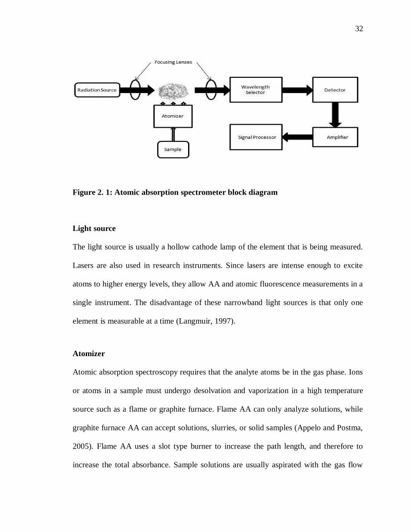
32
Figure 2. 1: Atomic absorption spectrometer block diagram
Light source
The light source is usually a hollow cathode lamp of the element that is being measured.
Lasers are also used in research instruments. Since lasers are intense enough to excite
atoms to higher energy levels, they allow AA and atomic fluorescence measurements in a
single instrument. The disadvantage of these narrowband light sources is that only one
element is measurable at a time (Langmuir, 1997).
Atomizer
Atomic absorption spectroscopy requires that the analyte atoms be in the gas phase. Ions
or atoms in a sample must undergo desolvation and vaporization in a high temperature
source such as a flame or graphite furnace. Flame AA can only analyze solutions, while
graphite furnace AA can accept solutions, slurries, or solid samples (Appelo and Postma,
2005). Flame AA uses a slot type burner to increase the path length, and therefore to
increase the total absorbance. Sample solutions are usually aspirated with the gas flow
33
into a nebulizing/mixing chamber to form small droplets before entering the flame (U.S
EPA, 1983).
The graphite furnace has several advantages over a flame. It is a much more efficient
atomizer than a flame and it can directly accept very small absolute quantities of sample.
It also provides a reducing environment for easily oxidized elements. Samples are placed
directly in the graphite furnace and the furnace is electrically heated in several steps to
dry the sample, ash organic matter, and vaporize the analyte atoms (Lester and Birkett,
1999). Light separation and detection AA spectrometers use monochromators and
detectors for UV and visible light. The main purpose of the monochromator is to isolate
the absorption line from background light due to interferences. Simple dedicated AA
instruments often replace the monochromator with a band pass interference filter.
Photomultiplier tubes are the most common detectors for AA spectroscopy (Appelo and
Postma, 2005).
Advantages and disadvantages of AAS
Atomic absorbtion spectroscopy present superior advantages over the other techniques
notably, solutions, slurries and solid samples can be analyzed much more efficient
atomization, high sensitivity [10-10g (flame), 10-14g (non-flame)], smaller quantities of
sample (typically 5 – 50 mL), provides a reducing environment for easily oxidized
elements, good accuracy (Relative error 0.1 ~ 0.5 % ), and Low detection limits. In
addition the techniques has a small turnaround time; of the order of few seconds.

34
However this technique has a number of demerits which include its low precision,
requires high level of operator skill, a resonance line source is required for each element
to be determined and its high cost of operation which makes it expensive. Due to its
simplicity, accuracy and sensitivity among other advantages, AAS will be preferred to the
other analytical techniques in this research.
35
CHAPTER THREE
MATERIALS AND METHODS
3.1 Study area
Athi River forms part of Athi-Galana River which is the second longest river in Kenya
(after the Tana River). It has a total length of 390 km, and drains a basin area of 70,000
km2. The river rises in 1° 42' S. as Athi River and enters the Indian Ocean as Galana
River (Asante et al., 2005). It flows across the Kapote and Athi plains, through the Athi
River town, takes a northeast direction and is met by the Nairobi River. Near Thika it
forms the Fourteen Falls and turns south-southeast under the wooded slopes of the Yatta
ridge, which shuts in its basin on the east. Apart from the numerous small feeders of the
upper river, almost the only tributary of significance is the Tsavo River, from the east
side of Kilimanjaro, which enters in about 3° S. It turns east, and in its lower course,
known as the Sabaki (or Galana), traverses the sterile quartz land of the outer plateau.
The valley is in parts low and flat, covered with forest and scrub, and containing small
lakes and backwaters connected with the river in the rains. Diring the rainy season the
stream, which rises as much as 9 meters. in places, is deep and strong and of a turbid
yellow colour; but navigation is interrupted by the Lugard falls, which is actually a series
of rapids. Onwards it flows east and enters the Indian Ocean in 30 12' S., just north of
Malindi (Akpabli, and Drah, 2001).
This river has numerous uses not only to the habitats of areas around the river banks but
also to the industrial sector. For these habitats, the river is useful as a source of water for
36
agricultural irrigation and domestic uses. For industrial purpose, it is used as a major
solvent for chemicals; it is also used as coolant especially in the smelter industries. It is
used for large scale production of horticultural products (Asante et al., 2005). The river
flows through the Tsavo East National Park and attracts diverse wildlife, including
hippopotamus and crocodiles.
Athi-Sabaki River basins in general experience two rainfall seasons controlled by the
Southern and Northern monsoons (Ojany and Ogendo, 1986). The Southern monsoon is
associated with the long rains, which occur between March and June. However, in the
Kenya highlands the peak rainfall occurs in April. The Northern monsoon is associated
with the short rains that occur in the period between November and December with the
peak rainfall occurring in November. However, there are often large inter-annual
variations in rainfall, partly due to El-Nino and La-Nina southern oscillation phenomena.
While in Central Kenya highlands the annual rainfall is of the order 1500 mm compared
North coast which is in the order 900 mm per annum.
The Athi River basin harbors two of the main urban and industrial and agricultural areas
within Kenya.. These are, Nairobi city on the upper catchment areas, which is the heart of
industrial activities in Kenya. The second one is Malindi in the southeastern outlet of the
basin. In between, there are various economic activities, some of which are potential
sources of pollutants. High concentration levels of total suspended particulate matter
within the urban commercial area were associated with increased traffic volume.This was
in addition to long range transport of the pollutants from Industrial heating processes and

37
power generation at the beginning of industrial operations. The upper catchment area is
extensively used for urban settlement, transport and industrial activities while in the
southeastern parts it is heavily used for agricultural production especially livestock
keeping. The contribution of these land use activities to pollutants generation and hence
water pollution and quality degradation is quite enormous. The map of the study area is
shown in Figure 1.1.
Figure 3. 1: Map of the study area
38
3.2 Chemicals and reagents
The following are the reagents were used. All the reagents used were analytical
grade (A.G):
Phosphate buffer solution
Magnesium sulphate, Calcium chloride, Ferric chloride, potassium
dichromate, Mercuric Sulphate, Potassium hydrogen phthalate (KHP)
Sulphuric acid, hydrochloric acid and sodium hydroxide solution.
Glucoseglutamic acid solution.
Sample dilution water
Ferroin indicator solution
Standard ferrous ammonium sulphate (FAS), titrant
3.3 Materials/Apparatus
AAS ( MA 1700 Atomic Absorption Spectrophotometer)
Wavelength range: 170nm-900nm. Manufacture Guangzhou Maya equipment
co ltd.
pH Meter (HK-3C Table Model PH Meter ( Manufacturer, shenzhen datron
electronics co. )
TDS Meter (Hanna conductivity/TDS meter model HI 9835)
Conductivity meter (Probe: HI 76300 platinum 4-ring) (manufacture Hanna
Hanna labwear)

39
Thermometer (digital water Thermometer KT400 (China (Mainland))
manufacture shenzhen datron electronics co.
BOD bottles, 300 ml, and pointed ground glass stoppers.
Water bath.
Reflux flasks, consisting of 250 mL flask with flat bottom and with 24/29
ground glass neck
Condensers, 24/29 and 30 cm jacket Leibig or equivalent with 24/29 ground
glass joint, or air cooled condensers, 60 cm long, 18 mm diameter, 24/29
ground glass joint.
Hot plate.
Soil augar.
3.4Sampling
Samples of water and sediments were collected from Athi River, Kenya from samling
areas shown in Figure 1.1. The river is located in the heavily industrial region and
receives effluents from the .industries. Water was collected for determination of
physicochemical parameters and heavy metal contaminations. The sediments were
collected for heavy metal contaminations.
3.5 Sample collection
Nine sampling sites in the Athi River ecosystem were selected (S1 – S9). Sediments were
collected from targeted sites of Athi River banks, that is, at intervals of three kilometers.
Five sediment samples were collected from each site with a 6.5 cm diameter corer to a
40
depth of about 15 centimeters and placed into distinct polythene bags and labeled
according to the site of collection. These samples were kept in a deep freezer awaiting
analysis. Five water samples from each site were collected into 50 ml acid leached plastic
bottles which were then labeled according to the site of collection. Exactly 2ml of conc.
nitric acid was added to the water samples to inhibit any process which could change the
form of the heavy metals. In-situ measurement of temperature and pH was determined
intrusively with appropriate methods. Five water samples from the sampling points were
also collected for COD and BOD determinations; they were analyzed within 48 hours of
collection to avoid oxygen degradation.
3.6 Preparation of standards
A stock solution of 1000 mg/L containing Pb2+
, Cr2+
, Cu2+
, Cd2+
and Ni2+
were prepared.
They were prepared by dissolving 1.59g, 3.05g,2.67g, 2.1g and 2.103g of Pb(NO3)2,
CrCl2, CuCl2, Cd(NO3)2 and Ni(NO3)2, respectively in distilled water. Standards of 0, 2,
3, 4, and 5 mg/L for each metal ion were prepared and their absorbance determined using
AAS, from which calibration curve was plotted.
3.7 Sample preparation and experimental procedures
3.7.1 Sediment samples for heavy metal determination
The sediment samples were dried in an oven at 80°C for 24 hours. The dried sediment
samples were then ground using pestle and mortar till the desired fineness was achieved;
this was be mainly to increase the surface area for extraction of the heavy metals from the
sediment samples. The ground samples were then sieved using a sieve of mesh size 72
nm. A 0.5 g of each dry sample was weighed and placed in a clean Kjedahl flask to which

41
10 ml of aqua – regia solution was added, that is, a mixture of concentrated HNO3 with
concentrated HCl in the ration 1:3 was addeds The samples were digested using an
electric digester with glass fume exhaust for a stretch of 2 – 3 hours. The solution was
filtered using the normal filter papers (0.45 Whatman filter paper). Each of the resulting
clear solution was diluted to 100 ml using distilled water in acid cleaned volumetric
flasks. These solutions were ready for AAS analysis of heavy metals.
3.7.2 Water samples for heavy metal determination
Each sample was digested by adding 5ml of concentrated HNO3 acid in 250 ml beakers.
The samples were then digested by electric digester with glass fume exhaust for a stretch
of 2 hours after which they were evaporated to near dryness on a hot plate then gradually
cooled. After cooling, another 5ml HNO3 was added to each sample. The solutions were
then filtered using the normal filter papers. Each of the resulting clear solution was then
diluted to 100 ml using distilled water in acid cleaned volumetric flasks. These solutions
were ready for AAS analysis of heavy metals.
3.7.3 Water samples for BOD determination
BOD was determined as described by Sawyer and Mccarty, 1978. Samples can degrade
significantly during extended storage. To minimize sample degradation, and thus avoid
negative bias in the measurement of BOD, analysis of the water samples was done
promptly after sample collection. In order to minimize changes in bacterial concentration.
The BOD test procedure was based on DO concentration and required an accurate DO
42
determination. The procedure presented below incorporates the amperometric method for
determining DO concentration.
Pre – analysis treatment
Sample dilution water was prepared 3 to 5 days before initiating BOD tests to ensure that
the BOD of the dilution water was less than 0.2 mg/L. The sample pH was determined
and adjusted to a pH from 6.5 to 7.5 using (H2SO4) for samples with pH greater than 7.5
or by use of (NaOH) if the samples had a pH less than 6.5. Sodium sulphide (Na2SO3)
was then added to remove residual chlorine. Preliminary pretreatment was done to
remove any interfering arsenic or cyanide residues. Samples were seeded appropriately
after pretreatment.
BOD analysis determination.
A functional constant temperature chamber was turned on and its controlled temperature
allowed to stabilize at 20°C ±1°C by use of a thermometer. Dilution was done to obtain
samples with a residual DO (after 3 days of incubation) of at least 1 mg/L and a DO
uptake of at least 2 mg/L. Several dilutions was done using the recommended sample
volumes for the 5-day biochemical oxygen demand test. For preparation of dilution in
graduated cylinders, dilution water was siphoned and seeded into a 1 to 2 L capacity
cylinder. Siphoning was done slowly without bubbling, using a screw-pin on the tube to
regulate the flow. The tip of the tube was kept just below the water surface as it rises.
The cylinder was half filled, and a desired quantity of sample added then diluted to
43
appropriate level. The mixed diluted sample was siphoned in three BOD bottles and
stopper was tightly placed without entraining any air.
DO determination procedure
Initial DO was determined on one bottle and the other two incubated at 27°C. The final
DO was determined) in duplicate after 3 days. The DO was determined as follows: BOD
bottle containing the sample was drained off any liquid in the flared tip. The stopper was
removed and 1 mL of MnSO4 added followed by 1 mL sodium hydroxide-iodide-azide
reagent and then stoppered carefully to exclude air bubbles. The solution was mixed by
inverting the bottle a few times. The brown manganese hydroxide floc (white floc which
indicates absence of DO) was allowed to settle approximately to half the bottle volume
and then 1.0 mL concentrated H2SO4 was added and re-stopper. Rapid mixing of the
solution was done by inverting several times until dissolution was complete. 20 mL of
this standard mixture was titrated with standard sodium thiosulphate.
3.7.4 COD determination
This was determined as described by Munde et al., (2006). 50 ml of sample was taken
into a refluxing flask and several boiling stones was added. 0.1 g HgSO4 and 5 ml of
concentrated H2SO4 was added to the solution. To ensure that HgSO4 dissolved
completely, the solution was swirled slowly while adding H2SO4 0.1 g of Ag2SO4 was
added to this solution. Finally 0.2 M potassium dichromate was added. Thorough mixing
of the solution was confirmed by swirling the flask in a water bath to recover any volatile
substances that may have escaped from the liquid state. The flask was then attached to the
44
condenser and further cooling was done. 20 ml of H2SO4 was added to the solution in the
flask. The solution was refluxed for 1 hour.
A blank run (using 50 ml distilled water instead of sample) was simultaneously
conducted with the same procedure after cooling; the solution was transferred to an
Erlenmeyer flask. The reflux flask was rinsed thrice, pouring the rinsing water to the
Erlenmeyer flask. The solution was diluted to about 300 ml and about 8 drops of
phenanthroline ferrous sulphate was added to the solution as an indicator. The solution
was titrated against the Mohr’s salt and the titer volume required for the colour change
from blue-green to reddish blue was noted. The procedure was repeated for the blank run.
3.7.5 Analysis of pH
The pH was measured using a pH meter of a glass electrode. The pH meter glass
electrode was previously immersed in water for several hours. The measurement was
started 5 minutes after switching on the meter. The detecting unit was rinsed well with
water and water gently blotted with a piece of filter paper. The pH meter was adjusted at
one pH value and temperature compensation dial rotated to set to the temperature of the
pH standard solution. The detecting unit was then immersed in the pH standard solution
which had a pH near that of the sample solution, and after more than 2 minutes, adjusted
the zero point adjustment dial so that the reading of the pH meter is set to the pH of the
standard solution. The detecting unit was thoroughly washed with water, and gently
blotted with a piece of filter paper. The detecting unit was then immersed in the sample
solution and the pH value read.
45
3.7.6 Electrical conductivity
The electrical conductivity and total dissolved salts of the water was determined in a
quick and inexpensive way, using portable meters. The procedure as described by Wright
(2007), Water sample was collected with the container being entirely filled with the water
sample to exclude air and forwarded to a laboratory for testing within 24 hours since
delays and high temperatures could change the composition of salts in the sample,
affecting the results. The meter was calibrated, and then rinsed with deionized water. The
electrode was dipped into the sample and appropriate conductivity range selected. The
electrode was moved slowly in a circle for one minute until the digital read-out stabilizes
or continually jumped between two numbers. The results were recorded on results sheet.
3.8 Total dissolved solids
Samples were collected and analyzed within 36 hours to reduce biological activity, TDS
meter was calibrated rinsed at its tip and with distilled water. Then meter tip was placed
into water sample reading meter reading was taken. The meter was allowed to stabilize
before taking reading.
3.9 AAS Analysis
Atomic absorption spectrophotometer was used in the analysis. The concentrations of the
metals were determined in triplicates. The accuracy and precision of the analytical
procedure were determined. A series of standards were prepared for instrumental
calibration by serial dilution of working solutions (100 mg/L) prepared from analytical
grade stock solutions (1000 mg/L) from BDH Poole, USA. A standard and blank sample

46
was run after every seven samples to check for instrumental accuracy and calibration.
47
CHAPTER FOUR
RESULTS AND DISCUSSION
The mean heavy metal concentrations sampled in Athi River (in mg/L) was presented for
the generalization and therefore evaluation and assessment to be discussed in relation to
the findings, the state of this river. Physico-chemical water quality parameters; biological
oxygen demand, chemical oxygen demand, total suspended solids, conductivity and pH
were also analyzed and discussed.
4.1 Heavy metal analysis
4.1.1 Calibration Curves for Heavy metals
Calibration curves for each heavy metal were set to ensure the accuracy of the Atomic
Absorption Spectrophotometer (AAS) and to establish that results of the determination
proper were true and reliable. Standards with concentration of 1-5.mg/L were set for the
calibration of the AAS. The calibration curve of well-prepared standards and an accurate
AAS should present as a linear curve. The data on the calibration for copper, chromium,
nickel, lead and cadmium are shown in appendix vi.
4.1.2 Heavy Metals distribution on flowing river water.
The result clearly indicated that heavy metal concentrations were commonly in the same
range with world river averages as reported by Martin, and Meybeck, (1979). The trend
in concentration of heavy metals along the river is as shown in the Figures 4.4 to Figure
4.6.. The data indicates that the copper concentrations are low. This could be due to low
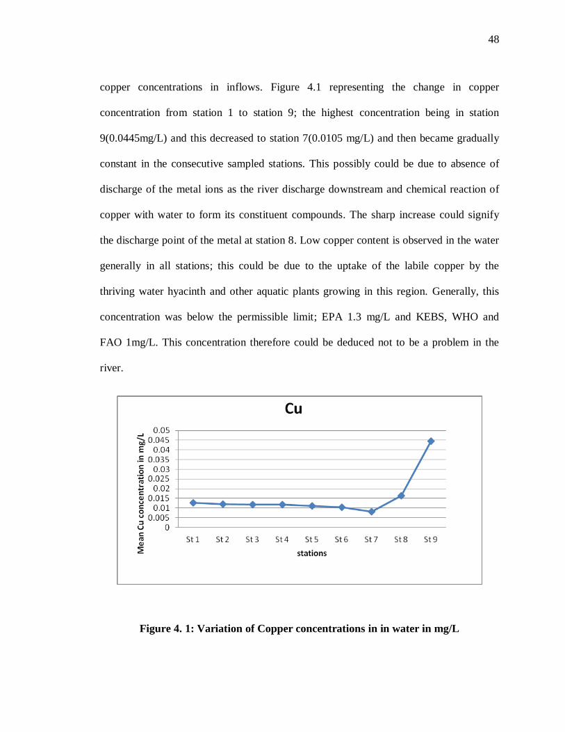
48
copper concentrations in inflows. Figure 4.1 representing the change in copper
concentration from station 1 to station 9; the highest concentration being in station
9(0.0445mg/L) and this decreased to station 7(0.0105 mg/L) and then became gradually
constant in the consecutive sampled stations. This possibly could be due to absence of
discharge of the metal ions as the river discharge downstream and chemical reaction of
copper with water to form its constituent compounds. The sharp increase could signify
the discharge point of the metal at station 8. Low copper content is observed in the water
generally in all stations; this could be due to the uptake of the labile copper by the
thriving water hyacinth and other aquatic plants growing in this region. Generally, this
concentration was below the permissible limit; EPA 1.3 mg/L and KEBS, WHO and
FAO 1mg/L. This concentration therefore could be deduced not to be a problem in the
river.
Figure 4. 1: Variation of Copper concentrations in in water in mg/L
49
The mean concentration of lead at the 9 different stations was as shown in Figure 4.2.
This measurement varied by fluctuating among the stations; rising from station 1(0.2444
mg/L) to 2(0.507 mg/L) and then fell to stations 4(0.237 mg/L). It then rose in station
5(0.47 mg/L), dropped in station 6, constant in 6 and 7 and finally rose in station
9(0.0446 mg/L). This fluctuation could probably be attributed to some industrial
discharge of their pollutants in the river. There was a battery recycling industry between
station 1 and 3, cement industry and steel industry between station 4 and 6 and finally
hides and skin between station 7 and 9. This concentration was also observed to be very
high compared to copper concentration. The high level of Pb in water of the river could
be attributed to the industrial and agricultural discharge as well as from spill of leaded
petrol from heavy trucks and dust which holds a huge amount of lead from the
combustion of petrol in automobile cars (Hardman et al., 1994) moreover higher levels of
Pb often occur in water bodies near highways and large cities due to high gasoline
combustion (Banat et al., 1998)..This concentration was also above the permissible limit
for FAO WHO (0.01mg/L) and KEBS (0.1 mg/L). Lead is therefore a pollutant of
concern in the river.

50
Figure 4. 2: Variation of lead concentrations in water in mg/L
Mean measurement of chromium concentration along the river (Figure 4.3) varied almost
similarly to that of lead with some slight increase from station 1(0.1892) to 2(0.2039
mg/L), dropped in station 4(0.1697 mg/L) rose to its highest at station 5(0.3255 mg/L)
after which it slightly registered an increase at station 8(0.1725 mg/L). The latter increase
can be attributed to effluent. Also, dust which holds a huge amount of lead from the
combustion of petrol in automobile cars led to increase Pb content (Hardman et al.
1994).This concentration is higher than the permissible limit for EPA (0.1mg/L), WHO
and FAO (0.01mg/L). The mean sampled concentration could also be deduced to be of
significant concern in the river in relation to biological communities.
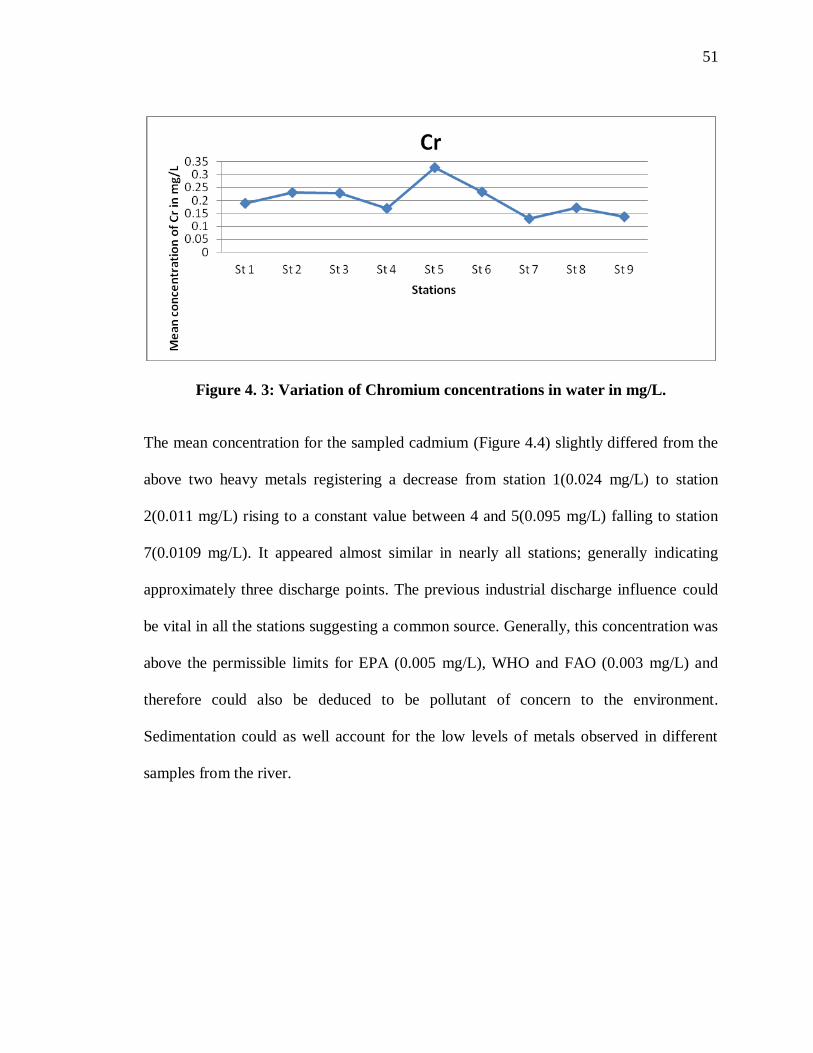
51
Figure 4. 3: Variation of Chromium concentrations in water in mg/L.
The mean concentration for the sampled cadmium (Figure 4.4) slightly differed from the
above two heavy metals registering a decrease from station 1(0.024 mg/L) to station
2(0.011 mg/L) rising to a constant value between 4 and 5(0.095 mg/L) falling to station
7(0.0109 mg/L). It appeared almost similar in nearly all stations; generally indicating
approximately three discharge points. The previous industrial discharge influence could
be vital in all the stations suggesting a common source. Generally, this concentration was
above the permissible limits for EPA (0.005 mg/L), WHO and FAO (0.003 mg/L) and
therefore could also be deduced to be pollutant of concern to the environment.
Sedimentation could as well account for the low levels of metals observed in different
samples from the river.
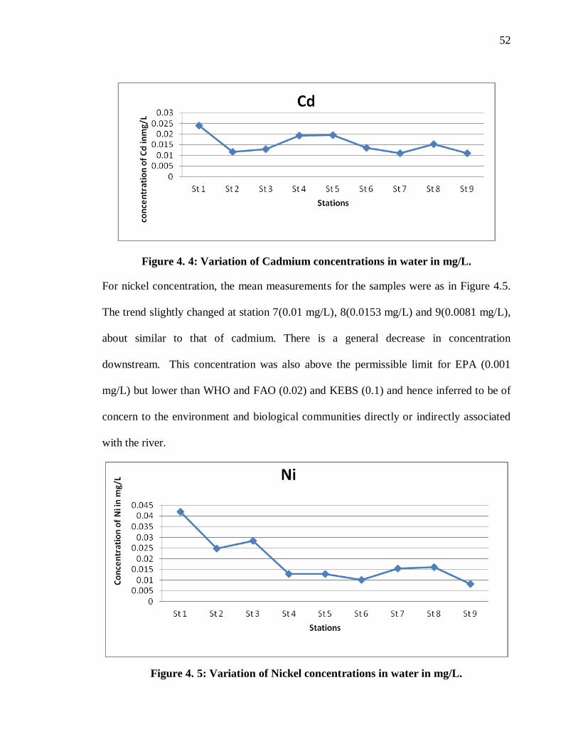
52
Figure 4. 4: Variation of Cadmium concentrations in water in mg/L.
For nickel concentration, the mean measurements for the samples were as in Figure 4.5.
The trend slightly changed at station 7(0.01 mg/L), 8(0.0153 mg/L) and 9(0.0081 mg/L),
about similar to that of cadmium. There is a general decrease in concentration
downstream. This concentration was also above the permissible limit for EPA (0.001
mg/L) but lower than WHO and FAO (0.02) and KEBS (0.1) and hence inferred to be of
concern to the environment and biological communities directly or indirectly associated
with the river.
Figure 4. 5: Variation of Nickel concentrations in water in mg/L.
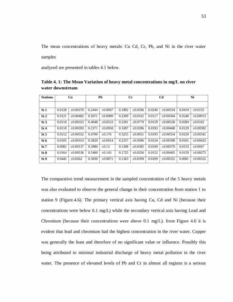
53
The mean concentrations of heavy metals: Cu Cd, Cr, Pb, and Ni in the river water
samples
analyzed are presented in tables 4.1 below.
Table 4. 1: The Mean Variation of heavy metal concentrations in mg/L on river
water downstream
Stations Cu Pb Cr Cd Ni
St 1 0.0128 ±0.00379 0.2444 ±0.0947 0.1892 ±0.0596 0.0240 ±0.00334 0.0419 ±0.0155
St 2 0.0121 ±0.00482 0.5071 ±0.0989 0.2309 ±0.0162 0.0117 ±0.00364 0.0248 ±0.00913
St 3 0.0118 ±0.00353 0.4048 ±0.0533 0.2281 ±0.0779 0.0129 ±0.00558 0.0284 ±0.0102
St 4 0.0118 ±0.00393 0.2371 ±0.0958 0.1697 ±0.0286 0.0193 ±0.00468 0.0129 ±0.00382
St 5 0.0112 ±0.00552 0.4700 ±0.176 0.3255 ±0.0931 0.0195 ±0.00354 0.0129 ±0.00341
St 6 0.0105 ±0.00353 0.3829 ±0.0914 0.2337 ±0.0586 0.0134 ±0.00308 0.0101 ±0.00423
St 7 0.0082 ±0.00137 0.3980 ±0.13 0.1308 ±0.0385 0.0109 ±0.00379 0.0153 ±0.0047
St 8 0.0164 ±0.00536 0.5400 ±0.143 0.1725 ±0.0356 0.0152 ±0.00465 0.0159 ±0.00275
St 9 0.0445 ±0.0262 0.3830 ±0.0871 0.1363 ±0.0399 0.0109 ±0.00322 0.0081 ±0.00322
The comparative trend measurement in the sampled concentration of the 5 heavy metals
was also evaluated to observe the general change in their concentration from station 1 to
station 9 (Figure.4.6). The primary vertical axis having Cu, Cd and Ni (because their
concentrations were below 0.1 mg/L) while the secondary vertical axis having Lead and
Chromium (because their concentrations were above 0.1 mg/L). from Figure 4.6 it is
evident that lead and chromium had the highest concentration in the river water. Copper
was generally the least and therefore of no significant value or influence. Possibly this
being attributed to minimal industrial discharge of heavy metal pollution in the river
water. The presence of elevated levels of Pb and Cr in almost all regions is a serious

54
matter of concern and the potential for human exposure to heavy metals from eating fish
caught in the river.
Figure 4. 6: The variation of all the tested heavy metals on river water in mg/L
Single ANOVA test reveal a significant difference in concentration of heavy metals
between different stations along the river and also between different heavy metals in the
river( p<0.05). These can be attributed to varying discharge points and difference in the
degree of discharge along the river.
4.1.3 Heavy metals in sediments
The mean concentration of copper in sediments was as observed in the Figure 4.7. This
was higher than that observed in water. The peaks was observed in station 4(0.1581
mg/L) and 9(0.2475 mg/L), falling through to station 2s while the lowest concentration
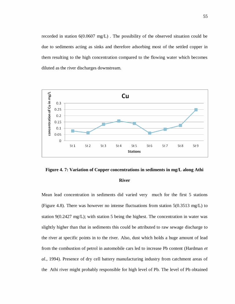
55
recorded in station 6(0.0607 mg/L) . The possibility of the observed situation could be
due to sediments acting as sinks and therefore adsorbing most of the settled copper in
them resulting to the high concentration compared to the flowing water which becomes
diluted as the river discharges downstream.
Figure 4. 7: Variation of Copper concentrations in sediments in mg/L along Athi
River
Mean lead concentration in sediments did varied very much for the first 5 stations
(Figure 4.8). There was however no intense fluctuations from station 5(0.3513 mg/L) to
station 9(0.2427 mg/L); with station 5 being the highest. The concentration in water was
slightly higher than that in sediments this could be attributed to raw sewage discharge to
the river at specific points in to the river. Also, dust which holds a huge amount of lead
from the combustion of petrol in automobile cars led to increase Pb content (Hardman et
al., 1994). Presence of dry cell battery manufacturing industry from catchment areas of
the Athi river might probably responsible for high level of Pb. The level of Pb obtained
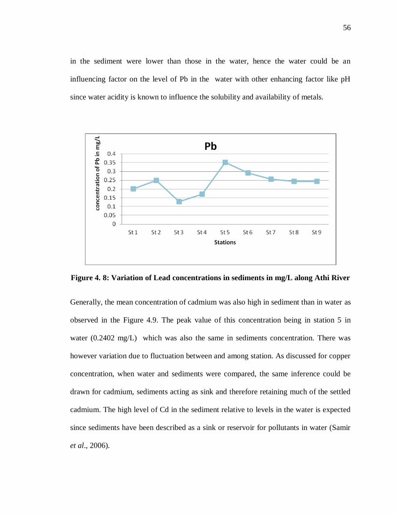
56
in the sediment were lower than those in the water, hence the water could be an
influencing factor on the level of Pb in the water with other enhancing factor like pH
since water acidity is known to influence the solubility and availability of metals.
Figure 4. 8: Variation of Lead concentrations in sediments in mg/L along Athi River
Generally, the mean concentration of cadmium was also high in sediment than in water as
observed in the Figure 4.9. The peak value of this concentration being in station 5 in
water (0.2402 mg/L) which was also the same in sediments concentration. There was
however variation due to fluctuation between and among station. As discussed for copper
concentration, when water and sediments were compared, the same inference could be
drawn for cadmium, sediments acting as sink and therefore retaining much of the settled
cadmium. The high level of Cd in the sediment relative to levels in the water is expected
since sediments have been described as a sink or reservoir for pollutants in water (Samir
et al., 2006).

57
Figure 4. 9: Variation of Cadmium concentrations in sediments in mg/L along Athi
River
The mean concentration for chromium in the sediments was lower than that in water
(Figure 4.10). The peak measurement in water was 0.3255 mg/L at station 5 and the
lowest being 0.1303 mg/L at station 1. Both of the concentration being above the
concentration of most stations (except for station 7) measurements at sediment
comparison. Possibly this can be attributed to active discharge of this heavy metal and
also with the lead above resulting to their concentration being high in water. The
industrial discharge could be frequently composed of these two heavy metals and
therefore high in water. The high level of Cd and Pb in sediments of Athi-River could be
attributed to the industrial and agricultural discharge as well as from spill of leaded petrol
from transportation lorries. Apparently the Cr-containing chemicals used for skin tanning
ends up in the environment the skin tunneling factory is located within two kilometers
from the river..
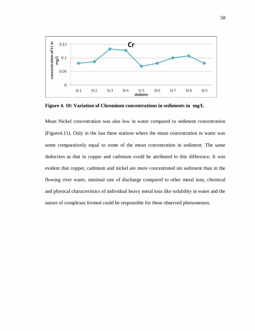
58
Figure 4. 10: Variation of Chromium concentrations in sediments in mg/L
Mean Nickel concentration was also low in water compared to sediment concentration
(Figure4.11). Only in the last three stations where the mean concentration in water was
some comparatively equal to some of the mean concentration in sediment. The same
deduction as that in copper and cadmium could be attributed to this difference. It was
evident that copper, cadmium and nickel are more concentrated sin sediment than in the
flowing river water, minimal rate of discharge compared to other metal ions, chemical
and physical characteristics of individual heavy metal ions like solubility in water and the
nature of complexes formed could be responsible for these observed phenomenon.
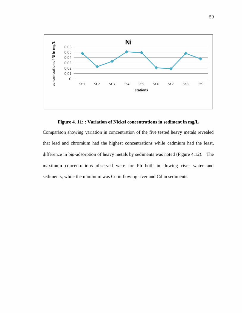
59
Figure 4. 11: : Variation of Nickel concentrations in sediment in mg/L
Comparison showing variation in concentration of the five tested heavy metals revealed
that lead and chromium had the highest concentrations while cadmium had the least,
difference in bio-adsorption of heavy metals by sediments was noted (Figure 4.12). The
maximum concentrations observed were for Pb both in flowing river water and
sediments, while the minimum was Cu in flowing river and Cd in sediments.
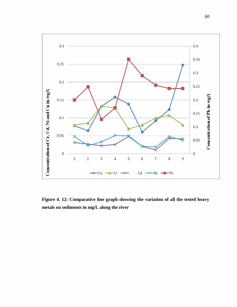
60
Figure 4. 12: Comparative line graph showing the variation of all the tested heavy
metals on sediments in mg/L along the river
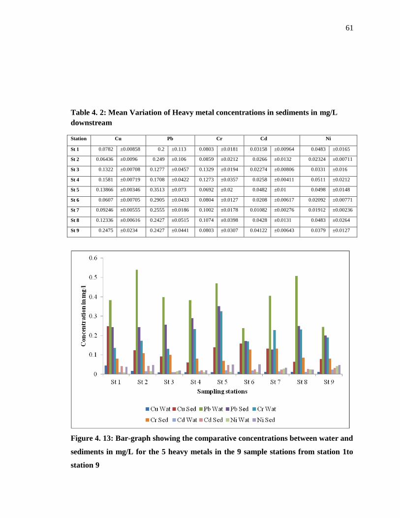
61
Table 4. 2: Mean Variation of Heavy metal concentrations in sediments in mg/L
downstream
Station Cu Pb Cr Cd Ni
St 1 0.0782 ±0.00858 0.2 ±0.113 0.0803 ±0.0181 0.03158 ±0.00964 0.0483 ±0.0165
St 2 0.06436 ±0.0096 0.249 ±0.106 0.0859 ±0.0212 0.0266 ±0.0132 0.02324 ±0.00711
St 3 0.1322 ±0.00708 0.1277 ±0.0457 0.1329 ±0.0194 0.02274 ±0.00806 0.0331 ±0.016
St 4 0.1581 ±0.00719 0.1708 ±0.0422 0.1273 ±0.0357 0.0258 ±0.00411 0.0511 ±0.0212
St 5 0.13866 ±0.00346 0.3513 ±0.073 0.0692 ±0.02 0.0482 ±0.01 0.0498 ±0.0148
St 6 0.0607 ±0.00705 0.2905 ±0.0433 0.0804 ±0.0127 0.0208 ±0.00617 0.02092 ±0.00771
St 7 0.09246 ±0.00555 0.2555 ±0.0186 0.1002 ±0.0178 0.01082 ±0.00276 0.01912 ±0.00236
St 8 0.12336 ±0.00616 0.2427 ±0.0515 0.1074 ±0.0398 0.0428 ±0.0131 0.0483 ±0.0264
St 9 0.2475 ±0.0234 0.2427 ±0.0441 0.0803 ±0.0307 0.04122 ±0.00643 0.0379 ±0.0127
Figure 4. 13: Bar-graph showing the comparative concentrations between water and
sediments in mg/L for the 5 heavy metals in the 9 sample stations from station 1to
station 9

62
Sed stands for sediments and wat stands for water in reverse order from station 1 to
station 9
There was a great significant difference between concentration of heavy metals in water
and concentration of heavy metals in sediments as evident by the ANOVA test h p>0.05.
This is possibly due to the different complexes formed by metal ions in sediments which
makes them immobile (Hamed, 1998). sewage discharge could also play a role since
they are discharged in the river before eventually getting in to the sediments. In general,
metal content in sediments is indicative of the degree of pollution and serves as a source
of solubilization into water depending on the physicochemical circumstances specifically
pH and temperature conditions and the uptake by benthic organisms (Ogoyi1, et al.,
2011). By comparing the accumulation of heavy metals in water and sediments, it can be
concluded that the heavy metals are highly accumulated in sediments than water, since
the sediments act as reservoir for all contaminants and dead organic matter descending
from the ecosystem above. Similar findings were reported by other authors (Hamed, 1998
and Nguyen et al., 2005). The positive correlations observed between most of the metals
in water, especially in Malindi, suggest relative uniformity of the sources of the metal
pollutants, as previously reported (Onyari and Wandiga, 1999). However, lack of a
similar degree of correlation among metals in the sediments of the habitats suggests that
the metals are retained differentially in the sediments. The high levels of metals in the
sediments and low level in the water at sites may be due to the calm (undisturbed) nature
of the area and therefore the particles are bound to settle.
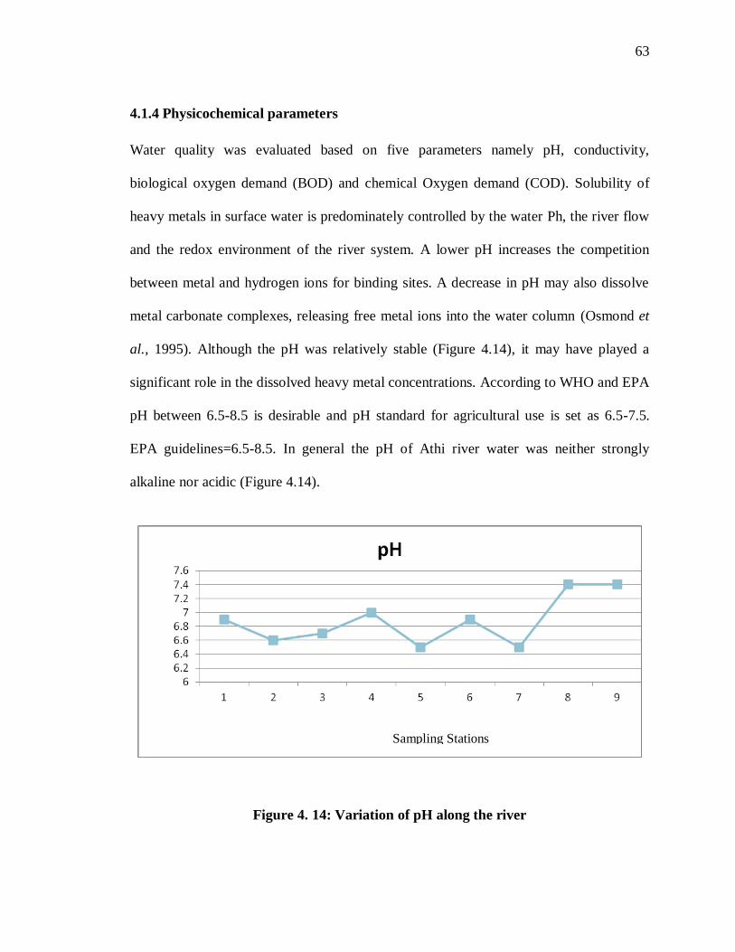
63
4.1.4 Physicochemical parameters
Water quality was evaluated based on five parameters namely pH, conductivity,
biological oxygen demand (BOD) and chemical Oxygen demand (COD). Solubility of
heavy metals in surface water is predominately controlled by the water Ph, the river flow
and the redox environment of the river system. A lower pH increases the competition
between metal and hydrogen ions for binding sites. A decrease in pH may also dissolve
metal carbonate complexes, releasing free metal ions into the water column (Osmond et
al., 1995). Although the pH was relatively stable (Figure 4.14), it may have played a
significant role in the dissolved heavy metal concentrations. According to WHO and EPA
pH between 6.5-8.5 is desirable and pH standard for agricultural use is set as 6.5-7.5.
EPA guidelines=6.5-8.5. In general the pH of Athi river water was neither strongly
alkaline nor acidic (Figure 4.14).
Figure 4. 14: Variation of pH along the river
Sampling Stations

64
The was no significant difference in pH (p<0.05) among the sampling locations. The pH
values of the various samples investigated ranged between 6.5 to 7.4. The results showed
both alkaline and acidic points along the river. This notwithstanding all results obtained
fell within national and international standard, EPA/WHO (6.5-8.5)
The BOD values (Figure 4.15) are all higher than the normal BOD for unpolluted water
of 2mg/L or less, a decreased redox potential, as is often seen under oxygen deficient
conditions, will change the composition of metal complexes and release the metal ions
into the overlying water. There was a positive correlation between heavy metal
concentration and BOD along the river possibly because metal ions consume oxygen
during the oxidation process. This variation in the rivers sediment was reflected on the
metals distribution. This in agreement with Franc et al., 2005 and Tsai et al., 2003 who
mentioned that sediments contain more sand and lower values of organic matter exhibit
low metals enrichment. They also observed from their findings that the pollutant
concentrations in sediments increased with decreasing the particle size in sediments.
Sediment has certain limited capacity to absorb different ions from waters percolating
through it. This capacity is lowest for carbonate-sandy fractions of sediments (Lake-sea
area), and highest for organic matter rich sediments. As the river re-aerates due to
atmospheric mixing and as algal photosynthesis adds oxygen to the water, the oxygen
levels will slowly increase downstream. The World Health Organization recommended a
BOD limit of 6 mg/L and 3 mg/L in urban areas for drinking water. The BOD values in
this study ware all beyond this requirement possiply due to high concentrations of metal
ion which consume oxygen during the oxidation process.
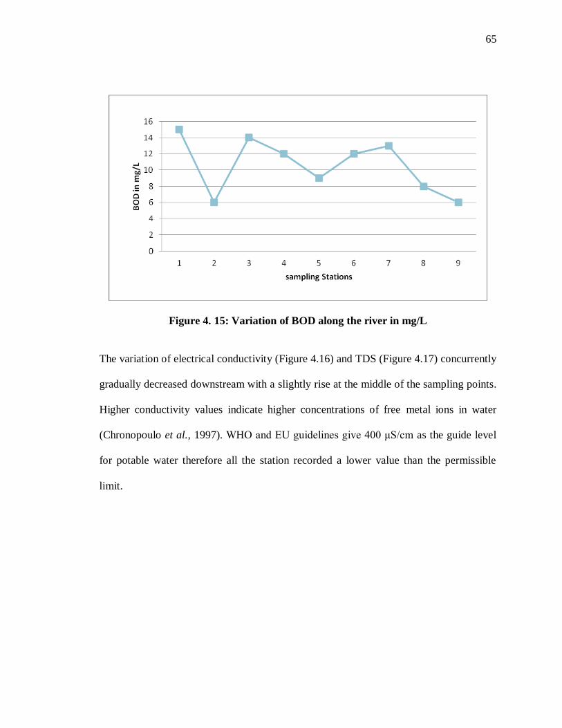
65
Figure 4. 15: Variation of BOD along the river in mg/L
The variation of electrical conductivity (Figure 4.16) and TDS (Figure 4.17) concurrently
gradually decreased downstream with a slightly rise at the middle of the sampling points.
Higher conductivity values indicate higher concentrations of free metal ions in water
(Chronopoulo et al., 1997). WHO and EU guidelines give 400 μS/cm as the guide level
for potable water therefore all the station recorded a lower value than the permissible
limit.
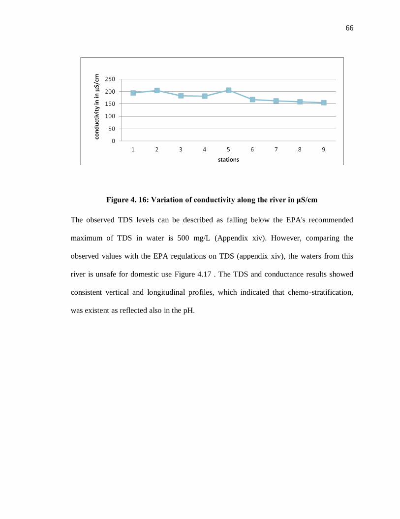
66
Figure 4. 16: Variation of conductivity along the river in μS/cm
The observed TDS levels can be described as falling below the EPA's recommended
maximum of TDS in water is 500 mg/L (Appendix xiv). However, comparing the
observed values with the EPA regulations on TDS (appendix xiv), the waters from this
river is unsafe for domestic use Figure 4.17 . The TDS and conductance results showed
consistent vertical and longitudinal profiles, which indicated that chemo-stratification,
was existent as reflected also in the pH.
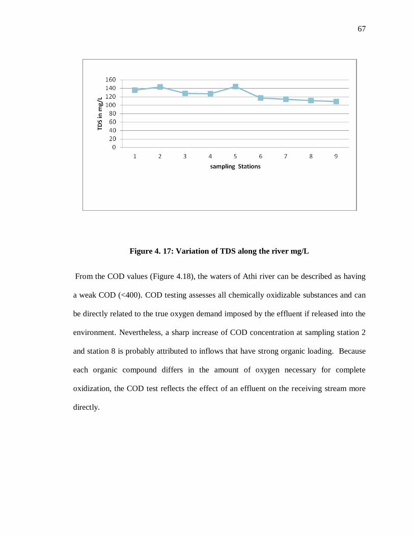
67
Figure 4. 17: Variation of TDS along the river mg/L
From the COD values (Figure 4.18), the waters of Athi river can be described as having
a weak COD (<400). COD testing assesses all chemically oxidizable substances and can
be directly related to the true oxygen demand imposed by the effluent if released into the
environment. Nevertheless, a sharp increase of COD concentration at sampling station 2
and station 8 is probably attributed to inflows that have strong organic loading. Because
each organic compound differs in the amount of oxygen necessary for complete
oxidization, the COD test reflects the effect of an effluent on the receiving stream more
directly.

68
Figure 4. 18: Variation of COD along the river mg/L
The environmental quality standards for surface water demands COD value to be < 30
mg/l. and therefore the athi river water were all above the recommended COD value.
Figure 4. 19: Comparison between BOD and COD in mg/L
The COD values ware higher than BOD values (figure 4019). The difference is not
surprising since COD measures both oxidizable organic and inorganic substances while
COD
BOD

69
BOD measures only biologically active oxidizable substances. COD can also be used to
evaluate BOD these can be deduced from the general trend above. s
70
CHAPTER FIVE
CONCLUSION AND RECOMMENDATIONS
5.0 Conclusion
The investigation of heavy metal pollutants in Athi river namely Pb Cd, Cr, Cu and Ni
in free flowing water and within sediments of Athi River revealed that Pb was highest in
concentration in both free flowing water and sediments ranging from 0.2371 mg/L to
0.54 mg/L for water and 0.1277mg/L to 0.3513mg/L for sediments. The presence of
other heavy metals was also prominently observed.
Variation of average total dissolved solids, chromium, and lead concentrations ware
highest at industrial area. Copper mean concentration values were higher in sediments
ranging from 0.0643 mg/L to 0.2475 mg/L and lower free flowing water ranging from
0.0082 mg/L to 0.0445 mg/L .TDS and conductivity, had significant difference (P<0.05).
This implies that TDS and conductivity were the parameters of water quality of the river
that had been significantly affected by pollution. Most of the parameters in Athi River are
above those recommended by WHO, EPA and KEBS. The results of the study show that
although Athi River is already polluted from upstream activities, there is a significant
increase in the levels of BOD and TDS. This suggests strongly that human activities
along this river are partially contributing to its pollution thereby endangering the health
of the people who rely on the river as their water source and affecting the ecosystem too.
71
5.2 Recommendations
To improve the water quality and environment in the Athi River Basin, the following
should be done:
1. Rehabilitate and restore the river
2. Develop and implement water quantity and quality measuring protocols.
3. Enhance service delivery, environmental conservation, and sustainable use of
resources.
4. More of the untested heavy metals’ concentration should be conducted.
5. It is recommended that further periodic research should be done to continuously
monitor these indicators of pollution.
72
REFERENCES
Akpabli, C.K., and Drah, G.K. (2001). Water Quality of the Main Tributaries of the Athi
River. Journal of Chemistry, Science Association, 3:8494
Alkarahi, A., Ahmad, A., and Easa, A. (2009). Assessment of surface water quality of
selected estuaries of Kenya: multivariate statistical techniques. Environmentalist,
29, 255262.
Appelo, C.A.J. and Postma, D. (2005). Geochemistry, Groundwater and Pollution,
second ed. Balkema, Amsterdam. 649.
Asante K.A., Quarcoopome, T. and Amevenku, F.Y.K. (2005).Water Quality of the Athi
Reservoir after 10 years of Impoundment. East African Journal of Applied
Ecology, 13:171180.
Babiker I. S. and Mohamed, T. Hiyama. (2007). Assessing groundwater quality using
GIS. Water Resour Manage, 21:699–715.
Banat, I. M, Hassan, E. S., El-Shahawi, M. S. and Abu-Hilal, A. H . (1998). Post-gulf-
war assessment of nutrients, heavy metal ions, hydrocarbons, and bacterial
pollution levels in the United Arab Emirates coastal waters. Environ. Inter., 24
(2): 109–116.
73
Bates, R.G. (1973) Determination of pH: theory and practice. Pp 80.
Bencko, V. (1983). Nickel: A review of its occupational and environmental toxicology. J.
Hyg. Epidemic. Microorganism. Immunology. 27, 237.
Boyd, C.E. (1999). Water Quality: An Introduction. The Netherlands: Kluwer Academic
Publishers Group. ISBN 0-7923-7853-9.
BrodnjakVončina. D., Dobčnik, D. Sayari, A.,S. Hamoudi, S. (2002).Chemometrics
characterisation of the quality of river water.Analytical Chemistry, 462, 87100.
Burton, J. D and Liss, P. S. (1976).Estuarine Chemistry. Academic Press, London. p. 229
Carter, M. R. (1993). Soil Sampling and Methods of Analysis. Canadian Society of Soil
Science, Lewis, Boca Raton Pp 80.
Clair, N. S, Perry, L. M and Gene F. P (2003). Chemistry for Environmental Engineering
and Science (5th ed.). New York: McGraw-Hill. ISBN 0-07-248066-1
Clayton, G.D. and Patts C.F.E. (1994) Industrial Hygiene Toxicology, 4th ed.; A Wiley-
Interscience Publication: New York, pp 2157-2173.

74
Chronopoulos, J., Heidouti, C., Chronopoulou, S. A, and Massas, I. (1997). Variations in
plant and soil Lead and Cadmium content in urban parks in Athens, Greece. 196:
91-98.
Delzer, G.C., and McKenzie, S.W. (2003) Five day biochemical oxygen demand:
U.S.Pp150-200.
DeZuane, J. (1997). Handbook of Drinking Water Quality (2nd ed.). John Wiley and
Sons. ISBN 0-471-28789-X.
Dunbabin, J.S. and Bowmer, K.H. (1992). Potential use of constructed wetlands for
treatment of industrial wastewaters containing metals. The Science of the
Microbial remediation of metals. In R.L. Crawford Total Environment 111, 151–
68.
Ela, Wendell P.,(2007) Introduction to Environmental Engineering and Science, Prentice
Hall, 3rd ed. ISBN 0-13-148193-2.
EURACHEM,(2003). Quantifying Uncertainty in Analytical Measurement.Laboratory of
the Government Chemist, London.Pp 7-90.
75
Evans, E. H., and Giglio, J. (2000) Analytical Atomic Spectrom.,8 Geological Survey
Techniques of Water Resources Investigations, book 9, chap. A7 (3d ed.),
section 7.0, accessed 11th October 2011 from http://pubs.water.
Franc, S., Vinagre, I. C., and Henrique, C. N. (2005). Heavy metal concentrations in
sediment, benthic invertebrates and fish in three salt marsh areas subjected to
different pollution loads in the Tagus Estuary (Portugal). Baseline/Mar. Poll.
Bull., 50: 993–1018.,
Gibbs, R. J. (1970). Mechanisms controlling world water chemistry. Science, 170: 1088–
1090 .
Hamed, M. A. (1998). Distribution of trace metals in the River Nile ecosystem, Damietta
branch between Mansoura city and Damietta Province. J. Egypt. Ger. Soc. Zoo.,
27(A): 399-415.
Hardman, D. J., Mceldowney, S. and Watte, S. (1994). Pollution, ecology and
biotreatment. Longman Scientific, Technical, England, Pp322.
Harrison RM, Laxen DPH, Wilson SJ. (2007).Chemical associations of lead, cadmium,
copper, and zinc in street dusts and roadside soils. Environmental Science and
Technology.;15:1378–1383.

76
Hesterberg D. (1998).Biogeochemical cycles and processes leading to changes in
mobility of chemicals in soils. Agricultural Ecosystems Environ, 67: 121–133.
Hogan C.M and Marc, P. (1987). Development of a dynamic water quality simulation
model for the Truckee River, Earth Metrics Inc., Environmental Protection
Agency Technology Series, Washington D.C. Pp 50.
Hogan, C. M., Patmore, L. C. and Harry, S. (1973). Statistical Prediction of Dynamic
Thermal Equilibrium Temperatures using Standard Meteorological Data Bases.
EPA-660/2-73-003. U.S. Environmental Protection Agency Pp 80.
Isaac, F. (1956). "Use and Abuse of pH measurements". Analytical Chemistry 28 (12):
1859.
Iwashita, M., and Shimamura T., (2003), Long-term variations in dissolved trace
elements in the Sagami River and its tributaries (upstream area), Japan, The
Science of the Total Environment, 312, 167–179.
John, C. G. (1990). The Josephson Effects and Superconducting Electronics. CRC Press.
pp. 3, 20. ISBN 0-7503-0051-5.
Kingsley, O., Demas, A., Oteino and John, O. (1999). Sewage re-use for irrigation in
AthiRiver town Kenya: Its implications on public health .Volume 39, Issues 10–
11, 1999, Pages 343–346.

77
Kotti, M. E., Vlessidis, A. G., Wakida, F.T., and LaraRuiz J. (2005). Assessment of river
water quality in Eastern Kenya.Water Resource Management, 19, 77-94.
Kithiia and Mulei, S. (2006) The effects of land use types on the hydrology and water
quality of the Upper-Athi river basin, Kenya Pp 30.
Langmuir, D. (1997).Aqueous Environmental Geochemistry.Upper Saddle River, New
Jersey Prentice Hall, USA. Pp. 600-605.
Lawrence, S. P. and Don, R. K. (1994) Diamond: electronic properties and applications,
p. 140.
Lester, J. N. and Birkett, J. W. (1999).Microbiology and Chemistry for Environmental
Scientists and Engineers, 2nd edn.E and FN Spon, New York.Pp 200.
Markert, B. (1993). Plants as biomonitors for heavy metal pollution of concentrations.
Environ monitoring; 35:263.
Mcgregor D.B., Baan R.A., Partensky c., Rice J.M. and Wilbourn J.D. (2000). Evaluation
of the carcinogenic risks to humans associated with surgical implants and other
foreign bodies– a report of an IARC Monographs Programme Meeting. 36: 307-
313.
Martin, J.M. and Meybeck, M. (1979). Elemental mass balance of material carried by
major world rivers. 7: 173-206.
78
Mogere, (2005). Determination of concentration of total suspended particulate matter
and some gaseous air pollutants in Athi river urban area, in Kenya. University of
Nairobi Press.Pp 110.
Montaser, A. (1998), Inductively Coupled Plasma Mass Spectrometry.WileyVCH, New
York.Pp 7-50.
Moore W.A., Ludzack, F.J. and Ruchhoft, C.C. (1951). Determination of oxygen-
consumed values of organic wastes. Analytical Chemistry 23:1297.
Munde, W., Ganesh R. O. and Nguyen, D. H. (2006) Determination of Chemical Oxygen
Demand (COD) of Waste Water p.15-30.
Myers, R. J. (2010). "One-Hundred Years of pH". Journal of Chemical Education 87: 30.
DOI:10.1021/ed800002c.
Neal, C., Williams, R.J., Neal M., Bhardwaj, L.C., Wickham, H., Harrow, M. and Hill
L.K. (2000), The water quality of the River Thames at a rural site downstream of
Oxford, Science Total Enviroment..,252, 441–457.
Nyikuri,R.N, Oonge,Z.N and Odira,M.A. (2005) Trends in Heavy Metals Levels in the
Rivers of the Nairobi Region and Measures to Reduce them, journal of civivil
engineering reseach and practice 2 (2): ( 2005) PP 10-15.
79
Nguyen, H., M., Leermakers, J. O and S. Tfrfk W. B. (2005). Heavy metals in Lake
Balaton: water column, suspended matter, sediment and biota. Science Of the
Total Environment. 340: 213–230.
Ochieng, E.Z., Lalah J.O. and Wandiga S.O.(2009). Anthropogenic sources of heavy
metals in the Indian Ocean coast of Kenya. Oct;83(4):600-7.
Ogoyi1 D.O, Mwita C.J., Nguu E.K. and Shiundu P.M. (2011). Determination of
Heavy Metal Content in Water, Sediment and Microalgae from Lake Victoria,
East Africa. The Open Environmental Engineering Journal, 4, 156-161.
Onyari, J.M. andWandiga, S.O. (1999). Distribution of Cr, Pb, Cd, Zn, Fe and Mn in
Lake Victoria sediments, East Africa. Bull. Environ. Contam.
Toxicology;42:807–813.
Osmond, D.L., Line D.E., Gale J.A., Gannon R.W., Knott C.B., Bartenhagen K.A.,
Turner M.H.,Coffey S.W., Spooner J., Wells J., Walker J.C., Hargrove L.L.,
Foster M.A., Robillard ‘P.D.and Lehning D.W., (1995), Water, Soil and Hydro-
Environmental Decision Support System,
URL:www.water.ncsu.edu/watersheds/info /hmetals.html: Accessed on 20 Feb
2012.
80
Rajendra Prasad, D.S., Sadashivaiah, C. and Rangnna G. (2009). Hydrochemical
Characteristics and Evaluation of Groundwater Quality of Tumkur Amanikere
Lake Watershed, Karnataka, India. E-Journal of Chemistry, pp. 211-218.
Salt, D.E. and Kramer, U. (1998). Mechanisms of metal hyperaccumulation in plants. In:
RASKIN, I. and ENSLEY, B.D., eds. Phytoremediation of toxic metals: using
plants to clean up the environment. John Wiley and Sons, Inc., New York.
231246.Pp 50-90.
Sawyer, C. N. and McCarty, P. L. (1978) Chemistry for Sanitary Engineers 2nd Ed.
McGraw-Hill pp.394-399.
Samir, M.N., Mohamed, A.O. and Shaif, M.K., (2006). Environmental assessment of
heavy metal pollution in bottom sediments of Aden Port, Yemen. Int. J. Ocean
Oceanogr., 1(1): 99-109.
Singh A. K., Mondal, G.C, Suresh. K, Singh , B. K. and Sinha, A., (2008). Major ion
chemistry, weathering processes and water qua T. B. lity assessment in River
basins, Kenyan Environment Journal PP 745–758..
Tabachnick, B. G. and Fidell, S. (2007). Using Multivariate Statistics (5th ed.). Boston:
Pearson International Editio.PP 55-80.
81
Thuo, J .T ( 1991) Analysis of the levels of heavy metals in soil, plants, and urine samples
around the Athi River region. MSc University of Nairobi, Kenya.
Trygg, J., Wold, S. (2002). Orthogonal projections to latent sources of Heavy Metals
(OPLS).Pp 40.
Tsai, L. J., Ho S.T. and Yu.K.C. (2003). Correlation of extractable heavy metals with
organic matters in contaminated rivers sediments. Water Science and
Technology, 47: 101-107.
U.S Environmental Protection Agency.(1983). Methods for chemical analysis of water
and wastes, EPA600/ 479020.
USSL.(1954). Diagnosis and improvement of saline and alkali soils. USDA, Handbook,
60,147.
Vahter M., Berglund, M., Akesson, A.and Lidén C. (2002). Metals and women’s health.
Environmental Resources, 88: 145-155.
Verma B. L. and Srivastava R. N. (1990).Measurement of the Personal Cost of Illness
due to some Major Water related issues in an Indian Rural
Population.International Journal of Epidemiol, 19, 169–176.

82
Vončina, E., BrodnjakVončina, D., Gaillardet, and Viers. J. (2007).Chemometric
characterization of the quality of ground waters from different rivers in
Kenya.119-125.
Wolterbeek, H. T.(2002). Biomonitoring of trace element air pollution: principles,
possibilities and perspectives: Environmental Pollution. (Oxford, U. K.), 120,
1121.
World Health Organization (WHO).(2004). Guidelines for Drinking Water Quality.
Wright, M.R. (2007). An Introduction to Aqueous Electrolyte Solutions. Wiley.
ISBN 978-0-470-84293-5.
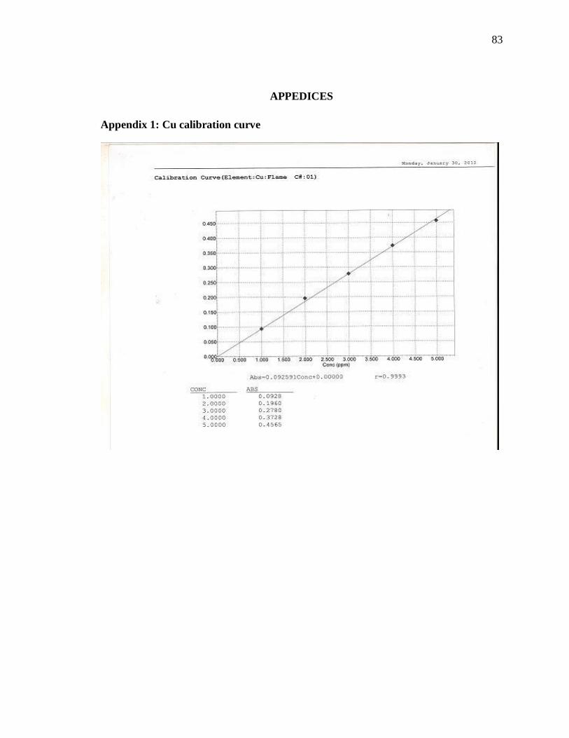
83
APPEDICES
Appendix 1: Cu calibration curve
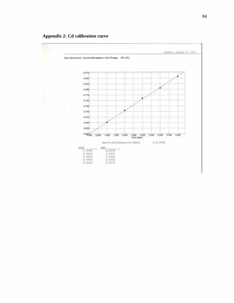
84
Appendix 2: Cd calibration curve
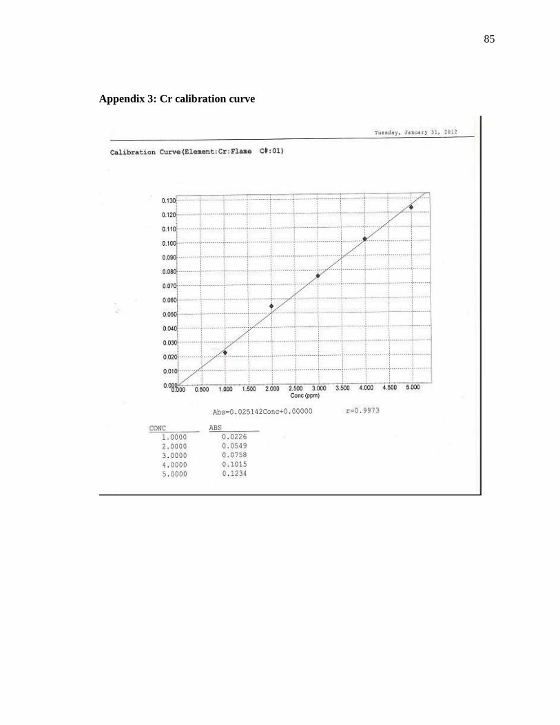
85
Appendix 3: Cr calibration curve
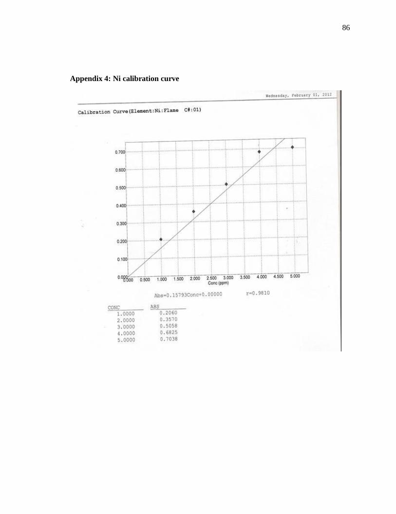
86
Appendix 4: Ni calibration curve

87
Appendix 5: Pb calibration curve
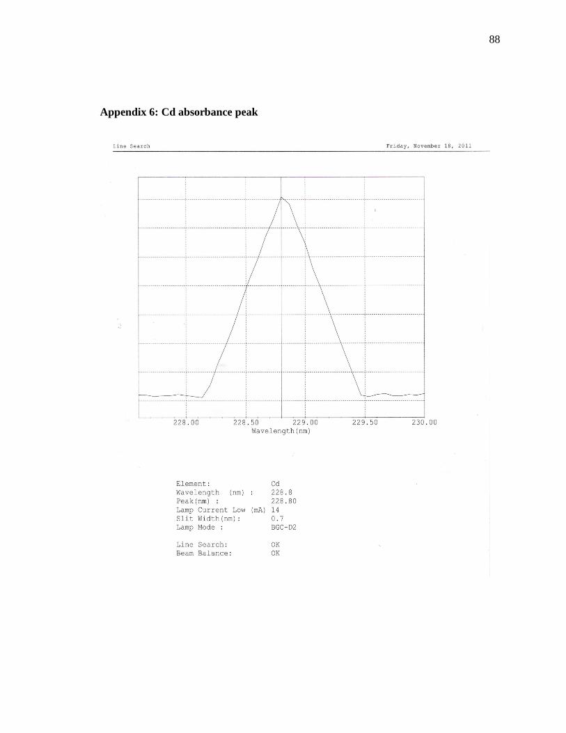
88
Appendix 6: Cd absorbance peak

89
Appendix 7: Cr absorbance peak
s
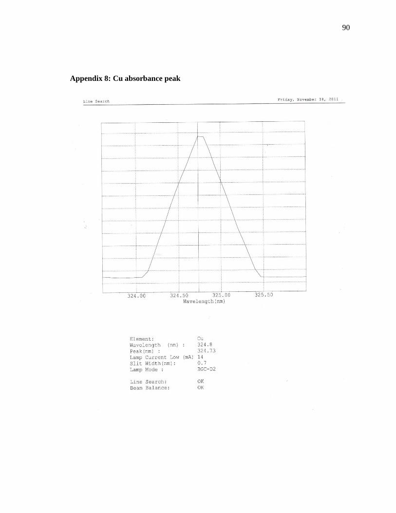
90
Appendix 8: Cu absorbance peak
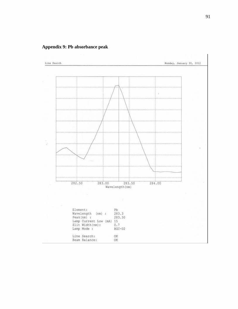
91
Appendix 9: Pb absorbance peak

92
Appendix 10: Ni absorbance peak
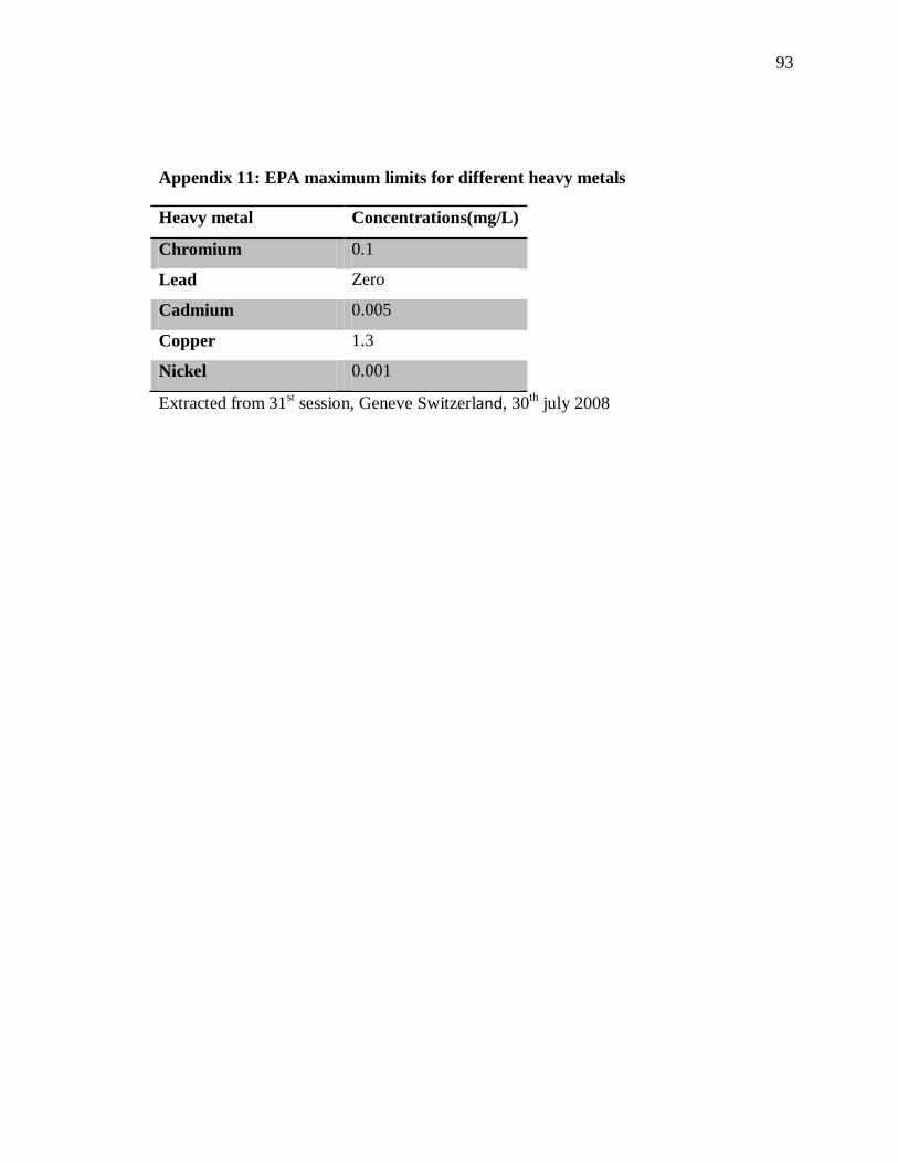
93
Appendix 11: EPA maximum limits for different heavy metals
Heavy metal Concentrations(mg/L)
Chromium 0.1
Lead Zero
Cadmium 0.005
Copper 1.3
Nickel 0.001
Extracted from 31st session, Geneve Switzerland, 30
th july 2008
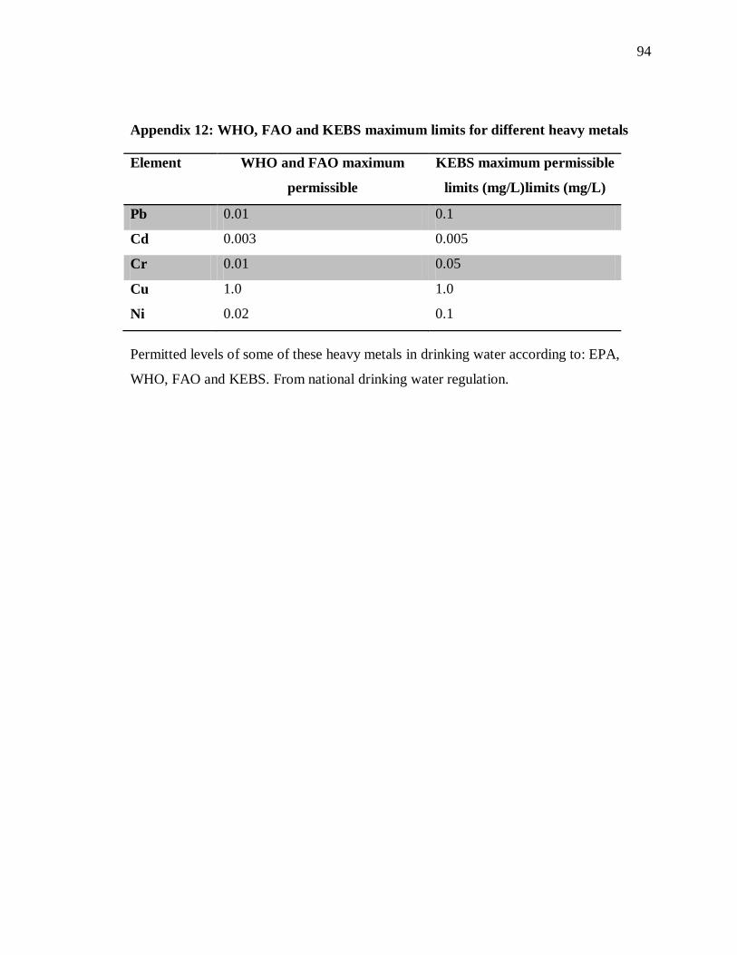
94
Appendix 12: WHO, FAO and KEBS maximum limits for different heavy metals
Element WHO and FAO maximum
permissible
KEBS maximum permissible
limits (mg/L)limits (mg/L)
Pb 0.01 0.1
Cd 0.003 0.005
Cr 0.01 0.05
Cu
Ni
1.0
0.02
1.0
0.1
Permitted levels of some of these heavy metals in drinking water according to: EPA,
WHO, FAO and KEBS. From national drinking water regulation.

95
Appendix 13: EPA regulations on TDS
Description Conc.(mg/L=ppm)
Ideal Drinking water from reverse osmosis, distillation,
deionization, microfiltration, etc..
050
Often considered acceptable range for carbon filtration,
mountain springs or aquifers.
50-140
Average tap water. 140-400
Hard water. 170 or above
Less desirable 200-300
Unpleasant levels from tap water, aquifers or mountain
springs.
300-500
The EPA's maximum contamination level. 500
Tolerance limits of TDS by KBS is 250 mg/L and pH 6.0-9.0, WHO TDS limits500 mg/L
Extracted from 31st session, Geneve Switzerland, 30
th july 2008
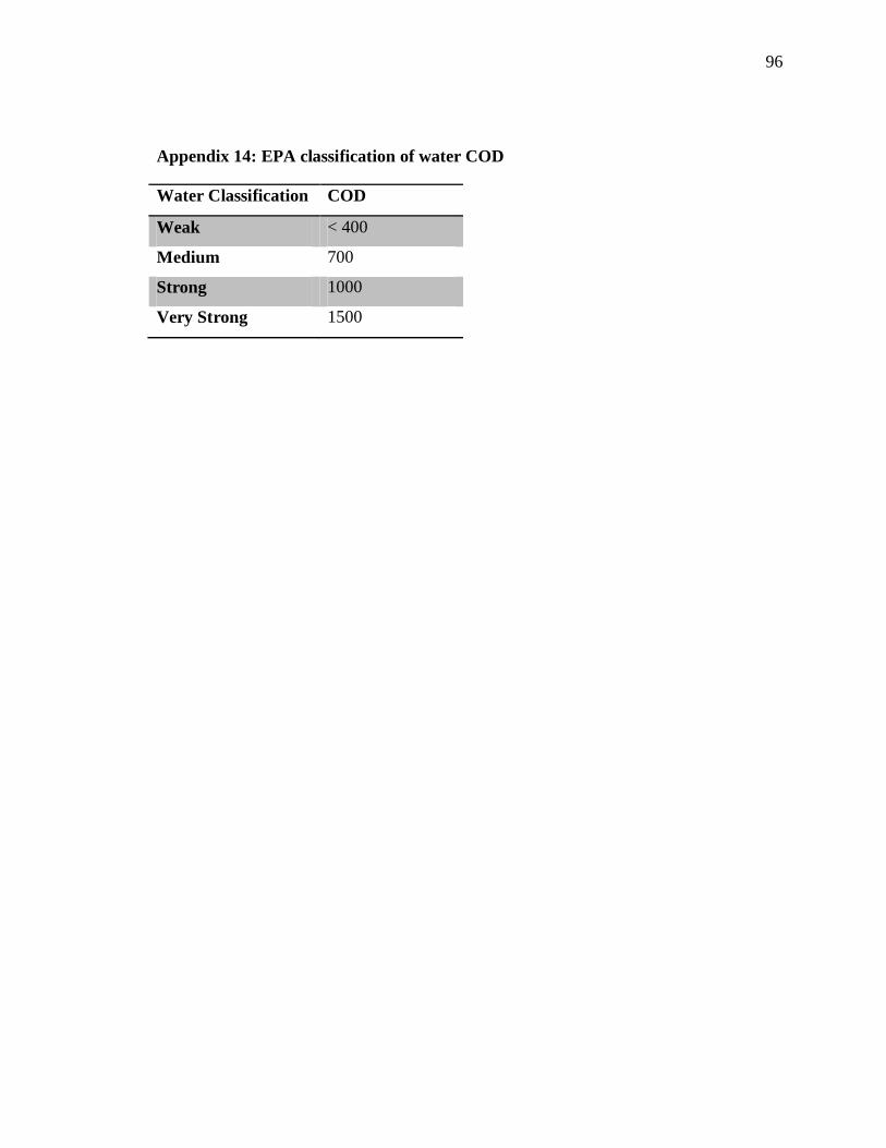
96
Appendix 14: EPA classification of water COD
Water Classification COD
Weak < 400
Medium 700
Strong 1000
Very Strong 1500


![NUCL 1 [512295]: Determination of heavy metals and …prosper.cofc.edu/~nuclear/2002Orlando223Abstracts.pdfNUCL 1 [512295]: Determination of heavy metals and their leaching characteristics](https://img.pdfslide.us/doc/110x75/5b2ba5ac7f8b9a594c8b7390/nucl-1-512295-determination-of-heavy-metals-and-nuclear2002orlando223abstractspdfnucl.jpg)