Determination of Sampling Plans Utilizing Risk Analysis

Jeff Hanson, ASQ CQE

Manager Technical Services

Upsher-Smith Laboratories, Inc.

When was the first time you were asked for a sampling plan?

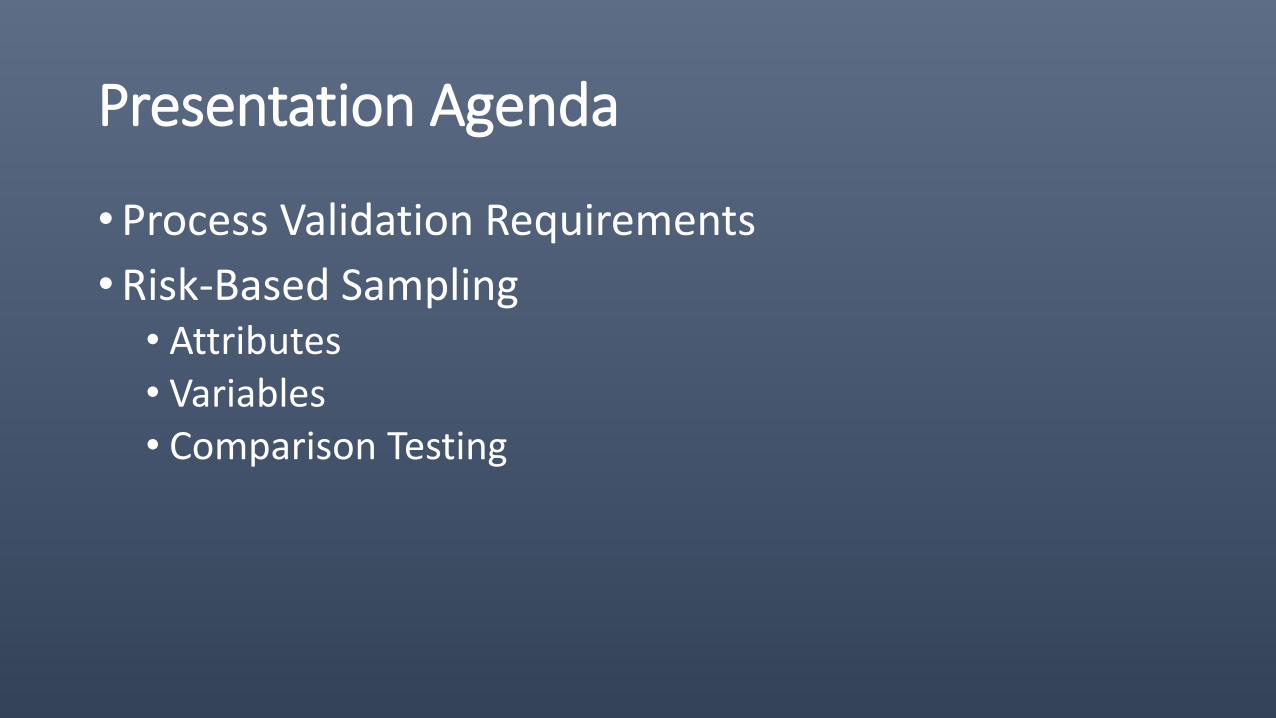
Presentation Agenda

•Process Validation Requirements

•Risk-Based Sampling • Attributes• Variables• Comparison Testing

Process Validation Requirements

1. “The sampling plan must result in statistical confidence”

2. “…samples must represent the batch under analysis.”

3. “The number of samples should be adequate to provide sufficient statistical confidence of quality both within and between batches. The confidence level selected can be based on risk analysis as it relates to the particular attribute under examination.”

Reference - Guidance For IndustryProcess Validation: General Principles and Practices

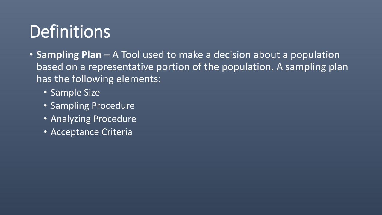
Definitions• Sampling Plan – A Tool used to make a decision about a population

based on a representative portion of the population. A sampling plan has the following elements: • Sample Size

• Sampling Procedure

• Analyzing Procedure

• Acceptance Criteria

Definitions

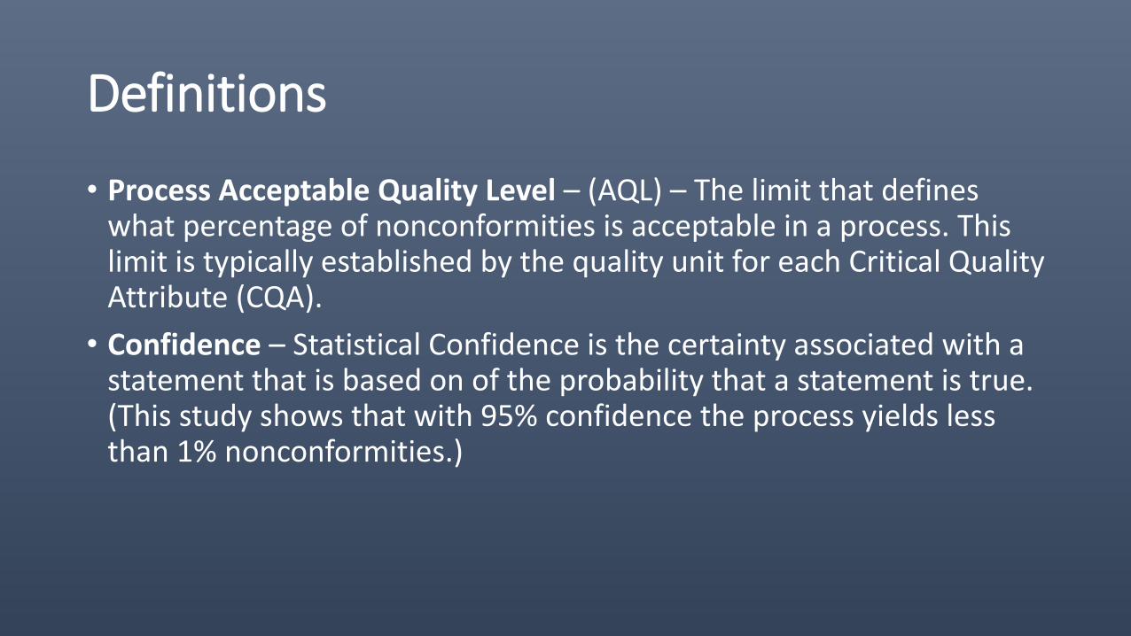
• Process Acceptable Quality Level – (AQL) – The limit that defines what percentage of nonconformities is acceptable in a process. This limit is typically established by the quality unit for each Critical Quality Attribute (CQA).

• Confidence – Statistical Confidence is the certainty associated with a statement that is based on of the probability that a statement is true. (This study shows that with 95% confidence the process yields less than 1% nonconformities.)

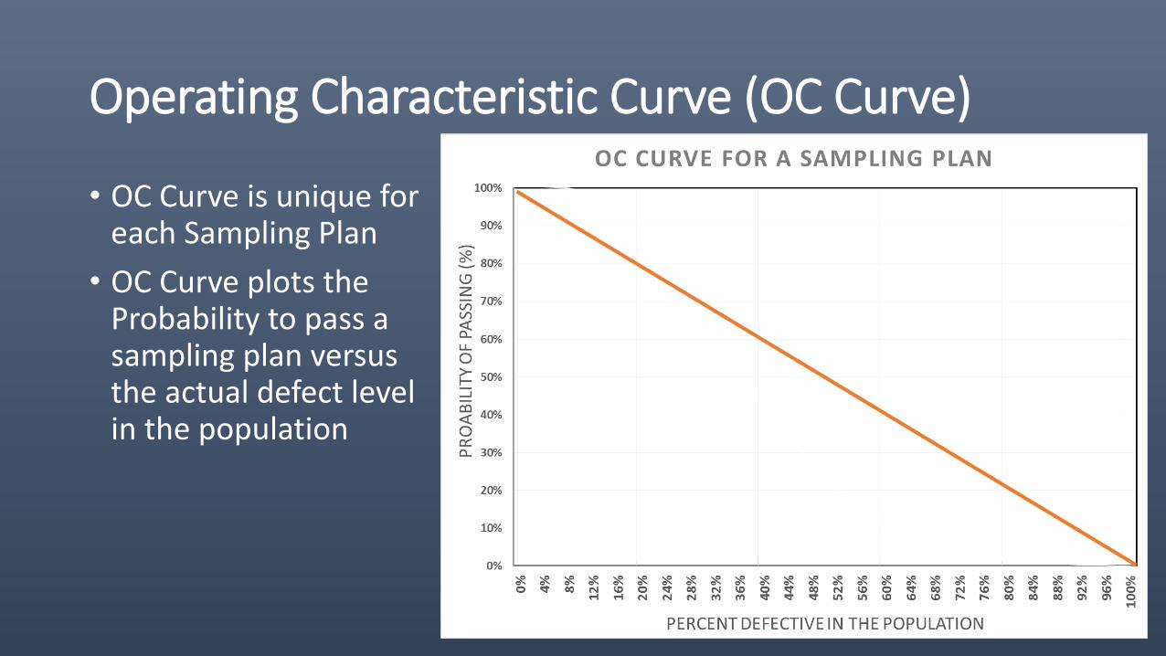
Operating Characteristic Curve (OC Curve)

• OC Curve is unique for each Sampling Plan

• OC Curve plots the Probability to pass a sampling plan versus the actual defect level in the population

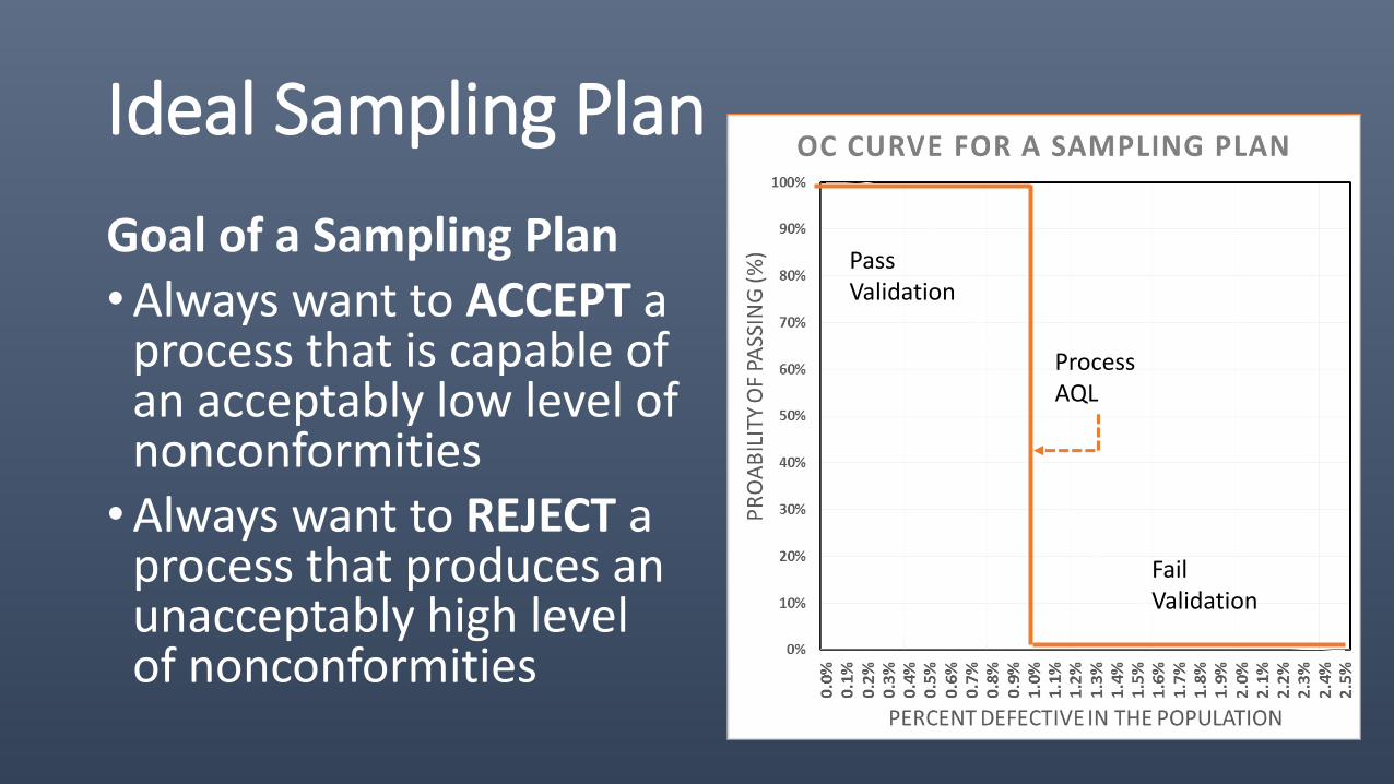
Ideal Sampling Plan

Goal of a Sampling Plan•Always want to ACCEPT a

process that is capable of an acceptably low level of nonconformities •Always want to REJECT a

process that produces an unacceptably high level of nonconformities

Pass Validation

Fail Validation

Process AQL

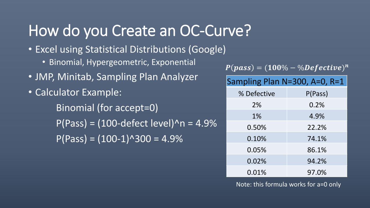
How do you Create an OC-Curve?• Excel using Statistical Distributions (Google)

• Binomial, Hypergeometric, Exponential

• JMP, Minitab, Sampling Plan Analyzer

• Calculator Example:

Binomial (for accept=0)

P(Pass) = (100-defect level)^n = 4.9%

P(Pass) = (100-1)^300 = 4.9%

Sampling Plan N=300, A=0, R=1

% Defective P(Pass)

2% 0.2%

1% 4.9%

0.50% 22.2%

0.10% 74.1%

0.05% 86.1%

0.02% 94.2%

0.01% 97.0%

𝑷 𝒑𝒂𝒔𝒔 = (𝟏𝟎𝟎% −%𝑫𝒆𝒇𝒆𝒄𝒕𝒊𝒗𝒆)𝒏

Note: this formula works for a=0 only

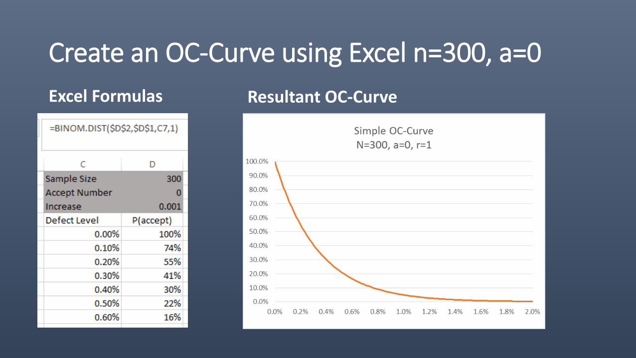
Create an OC-Curve using Excel n=300, a=0

Excel Formulas Resultant OC-Curve

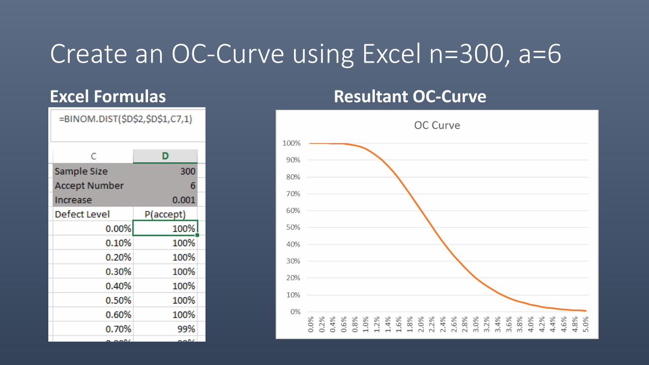
Create an OC-Curve using Excel n=300, a=6

Excel Formulas Resultant OC-Curve

Why do you create an OC-Curve?

“The confidence level selected can be based on risk analysis…”

• The OC-Curve shows us the elements of Risk that we need to consider to meet the three goals of a sampling plan• Want to Pass a capable process with high probability• Want to Fail a non-capable process with high probability• Want to state with adequate and predetermined

confidence that the process will yield acceptable quality product if it passes the sampling plan.

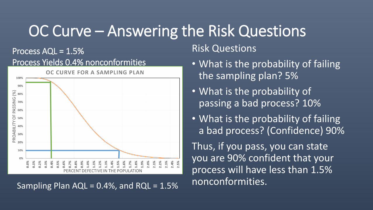
OC Curve – Answering the Risk QuestionsRisk Questions

• What is the probability of failing the sampling plan? 5%

• What is the probability of passing a bad process? 10%

• What is the probability of failing a bad process? (Confidence) 90%

Thus, if you pass, you can state you are 90% confident that your process will have less than 1.5% nonconformities.

Process AQL = 1.5%Process Yields 0.4% nonconformities

Sampling Plan AQL = 0.4%, and RQL = 1.5%

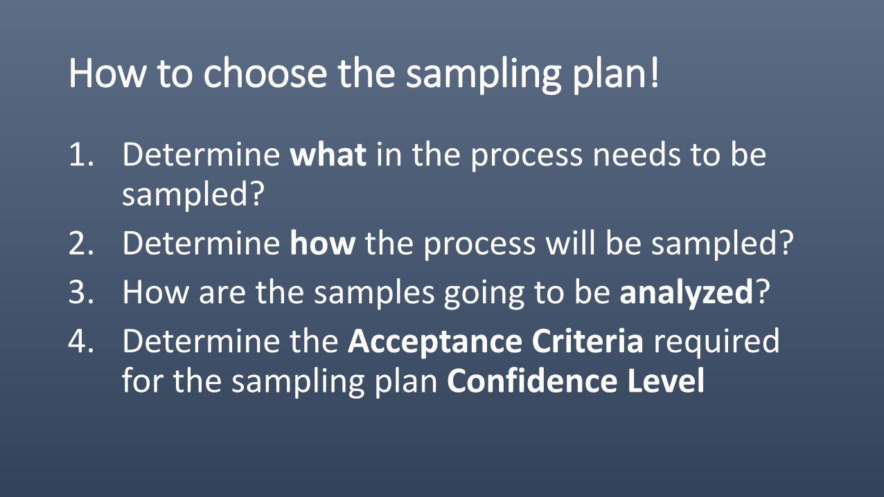
How to choose the sampling plan!

1. Determine what in the process needs to be sampled?

2. Determine how the process will be sampled?

3. How are the samples going to be analyzed?

4. Determine the Acceptance Criteria required for the sampling plan Confidence Level

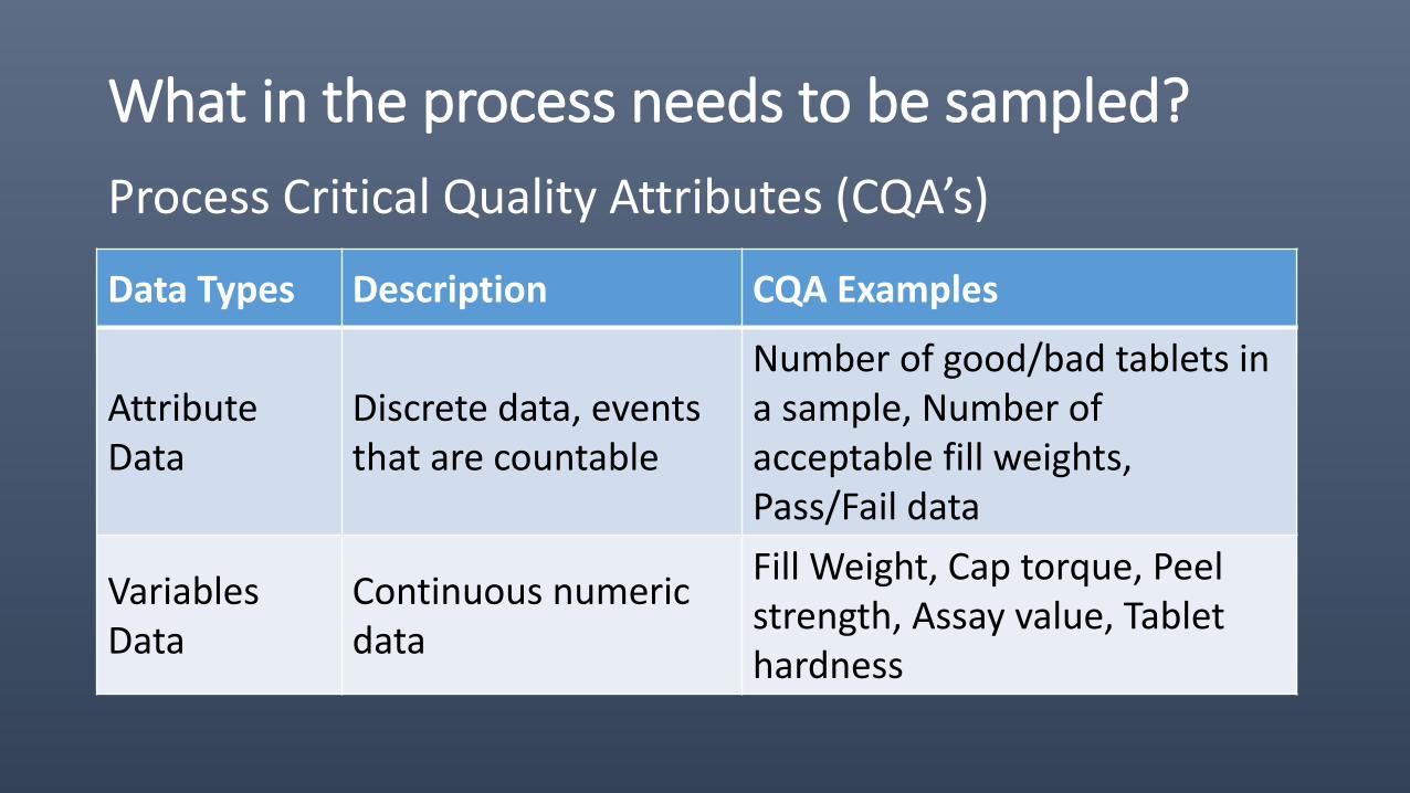
What in the process needs to be sampled?

Process Critical Quality Attributes (CQA’s)

Data Types Description CQA Examples

Attribute Data

Discrete data, events that are countable

Number of good/bad tablets in a sample, Number of acceptable fill weights, Pass/Fail data

Variables Data

Continuous numeric data

Fill Weight, Cap torque, Peel strength, Assay value, Tablet hardness

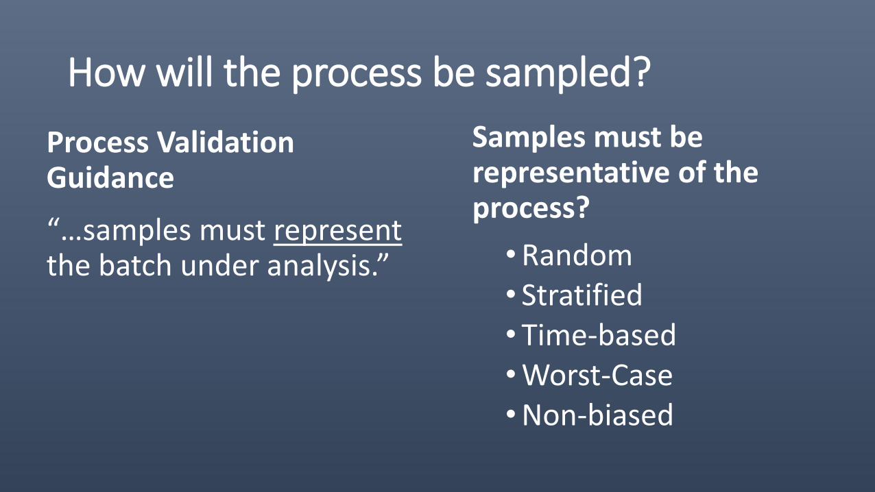
How will the process be sampled?

Samples must be representative of the process?

•Random• Stratified• Time-based•Worst-Case •Non-biased

Process Validation Guidance

“…samples must represent the batch under analysis.”

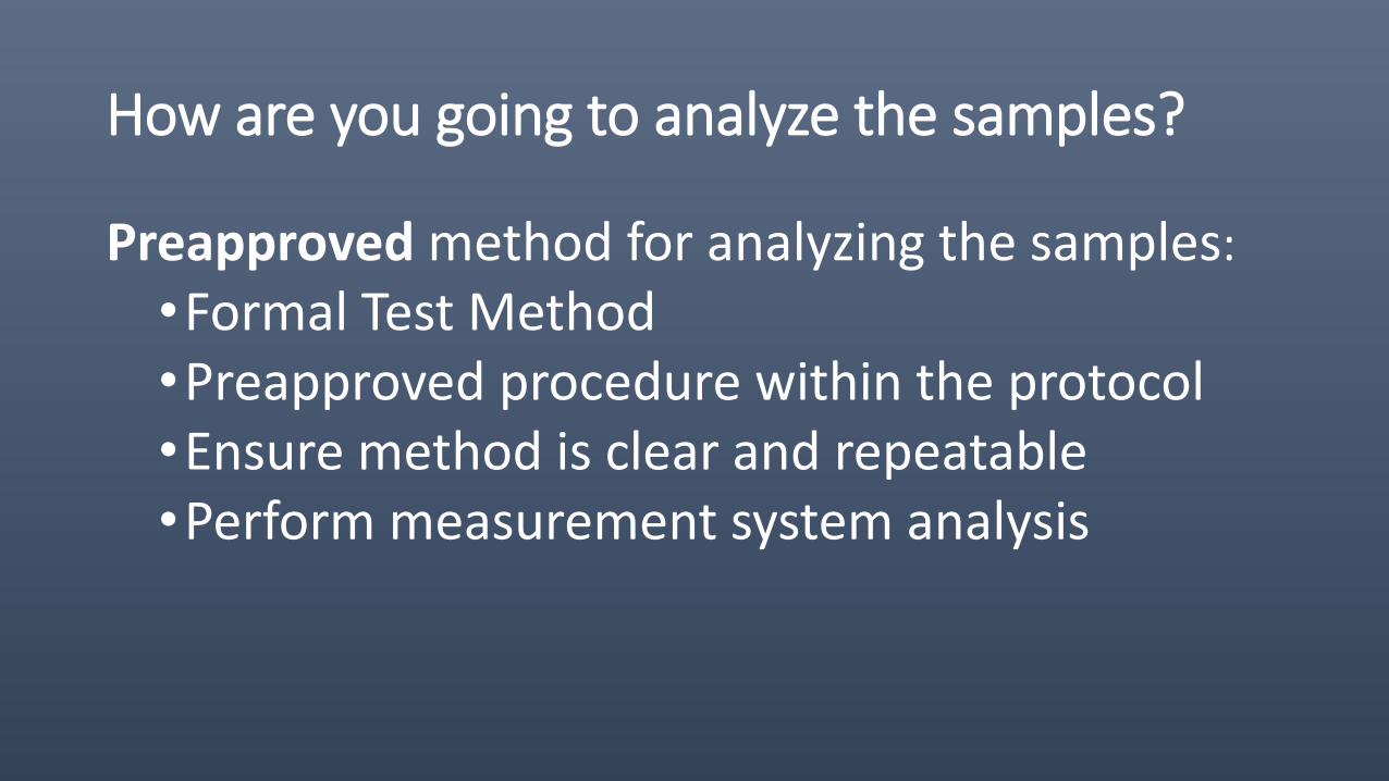
How are you going to analyze the samples?

Preapproved method for analyzing the samples:

•Formal Test Method•Preapproved procedure within the protocol•Ensure method is clear and repeatable•Perform measurement system analysis

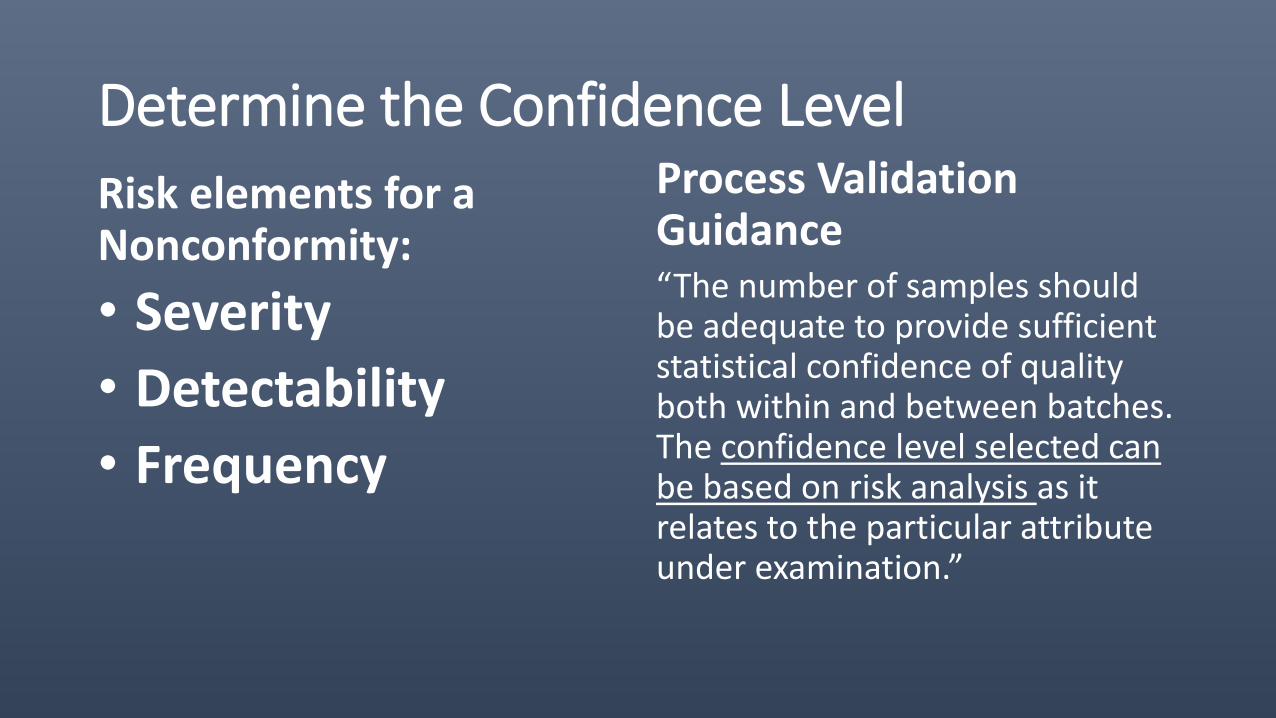
Determine the Confidence Level

Risk elements for a Nonconformity:

• Severity

• Detectability

• Frequency

Process Validation Guidance“The number of samples should be adequate to provide sufficient statistical confidence of quality both within and between batches. The confidence level selected can be based on risk analysis as it relates to the particular attribute under examination.”

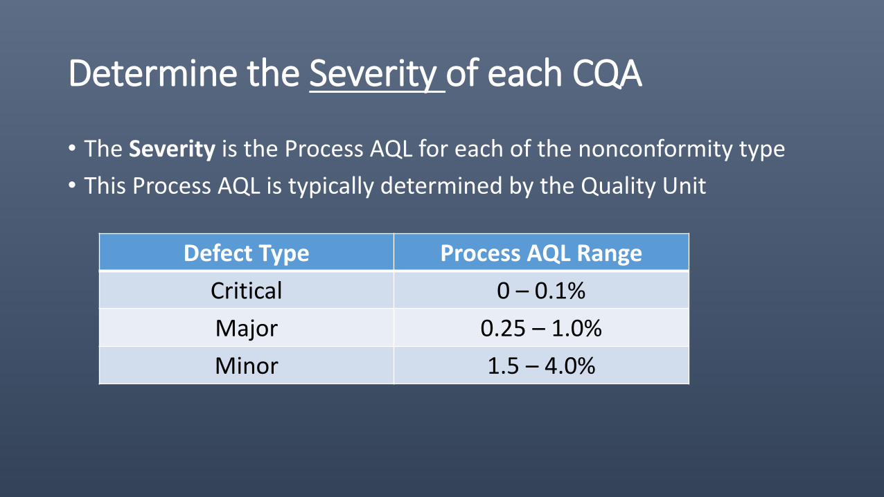
Determine the Severity of each CQA

• The Severity is the Process AQL for each of the nonconformity type

• This Process AQL is typically determined by the Quality Unit

Defect Type Process AQL Range

Critical 0 – 0.1%

Major 0.25 – 1.0%

Minor 1.5 – 4.0%

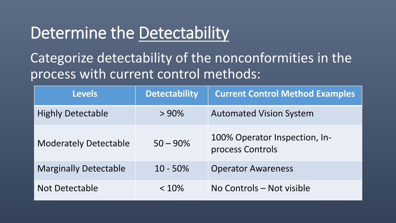
Determine the Detectability

Categorize detectability of the nonconformities in the process with current control methods:

Levels Detectability Current Control Method Examples

Highly Detectable > 90% Automated Vision System

Moderately Detectable 50 – 90%100% Operator Inspection, In-process Controls

Marginally Detectable 10 - 50% Operator Awareness

Not Detectable < 10% No Controls – Not visible

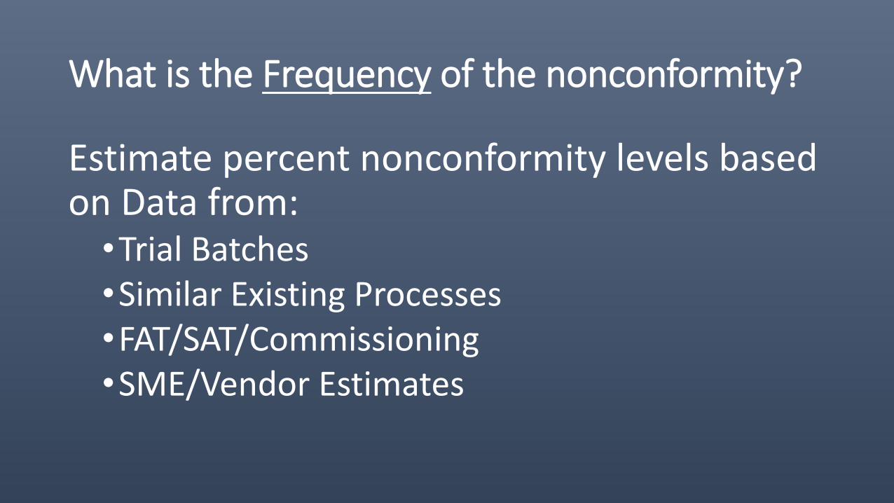
What is the Frequency of the nonconformity?

Estimate percent nonconformity levels based on Data from:•Trial Batches•Similar Existing Processes•FAT/SAT/Commissioning•SME/Vendor Estimates

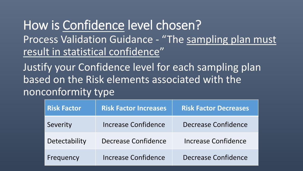
How is Confidence level chosen?Process Validation Guidance - “The sampling plan must result in statistical confidence”

Justify your Confidence level for each sampling plan based on the Risk elements associated with the nonconformity type

Risk Factor Risk Factor Increases Risk Factor Decreases

Severity Increase Confidence Decrease Confidence

Detectability Decrease Confidence Increase Confidence

Frequency Increase Confidence Decrease Confidence

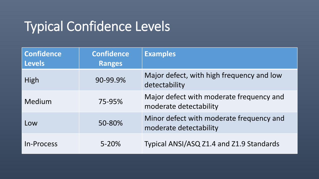
Typical Confidence Levels

ConfidenceLevels

Confidence Ranges

Examples

High 90-99.9%Major defect, with high frequency and low detectability

Medium 75-95%Major defect with moderate frequency and moderate detectability

Low 50-80%Minor defect with moderate frequency and moderate detectability

In-Process 5-20% Typical ANSI/ASQ Z1.4 and Z1.9 Standards

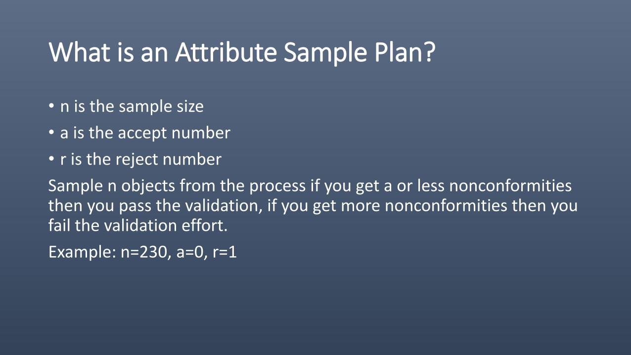
What is an Attribute Sample Plan?

• n is the sample size

• a is the accept number

• r is the reject number

Sample n objects from the process if you get a or less nonconformities then you pass the validation, if you get more nonconformities then you fail the validation effort.

Example: n=230, a=0, r=1

Choosing the Attribute Sampling Plan

• Confidence required (90%)

• Process AQL (1%)

• Frequency - Nonconformity Estimate (0.2%)

SampleSize (n)

Accept Number

(a)

Sampling Plan AQL

(%)

Sampling Plan RQL

(%)

230 0 0.02 1

388 1 0.09 1

531 2 0.15 1

667 3 0.21 1

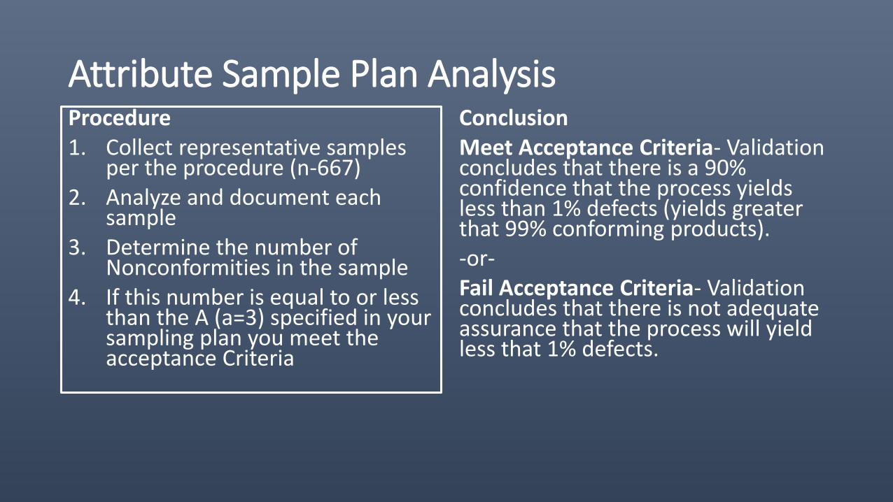
Attribute Sample Plan AnalysisProcedure1. Collect representative samples

per the procedure (n-667)2. Analyze and document each

sample3. Determine the number of

Nonconformities in the sample4. If this number is equal to or less

than the A (a=3) specified in your sampling plan you meet the acceptance Criteria

ConclusionMeet Acceptance Criteria- Validation concludes that there is a 90% confidence that the process yields less than 1% defects (yields greater that 99% conforming products).-or-Fail Acceptance Criteria- Validation concludes that there is not adequate assurance that the process will yield less that 1% defects.

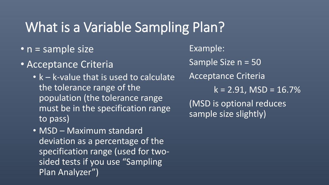
What is a Variable Sampling Plan?

• n = sample size

• Acceptance Criteria• k – k-value that is used to calculate

the tolerance range of the population (the tolerance range must be in the specification range to pass)

• MSD – Maximum standard deviation as a percentage of the specification range (used for two-sided tests if you use “Sampling Plan Analyzer”)

Example:

Sample Size n = 50

Acceptance Criteria

k = 2.91, MSD = 16.7%

(MSD is optional reduces sample size slightly)

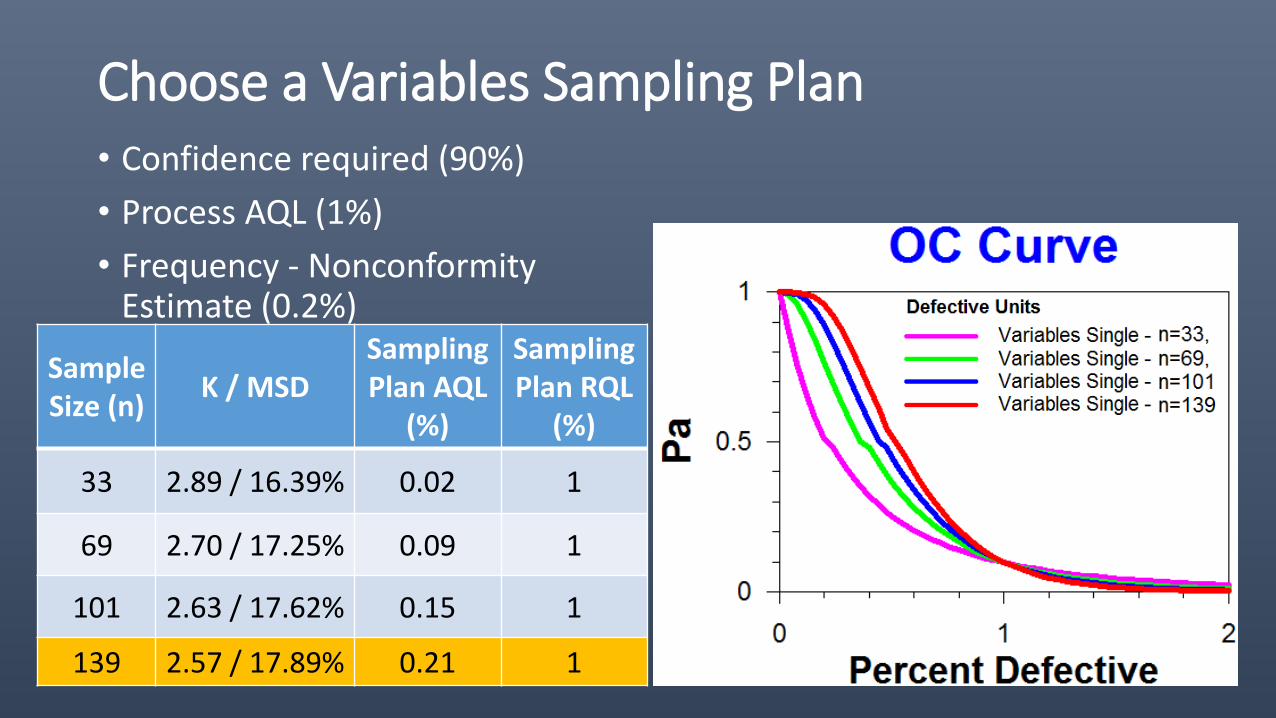
Choose a Variables Sampling Plan • Confidence required (90%)

• Process AQL (1%)

• Frequency - Nonconformity Estimate (0.2%)

SampleSize (n)

K / MSDSampling Plan AQL

(%)

Sampling Plan RQL

(%)

33 2.89 / 16.39% 0.02 1

69 2.70 / 17.25% 0.09 1

101 2.63 / 17.62% 0.15 1

139 2.57 / 17.89% 0.21 1

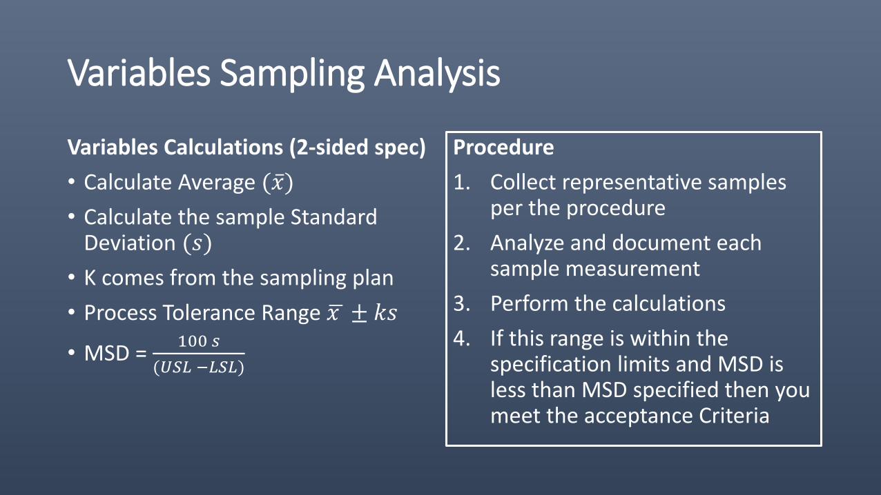
Variables Sampling Analysis

Variables Calculations (2-sided spec)

• Calculate Average ( 𝑥)

• Calculate the sample Standard Deviation (𝑠)

• K comes from the sampling plan

• Process Tolerance Range 𝑥 ± 𝑘𝑠

• MSD = 100 𝑠

(𝑈𝑆𝐿 −𝐿𝑆𝐿)

Procedure

1. Collect representative samples per the procedure

2. Analyze and document each sample measurement

3. Perform the calculations

4. If this range is within the specification limits and MSD is less than MSD specified then you meet the acceptance Criteria

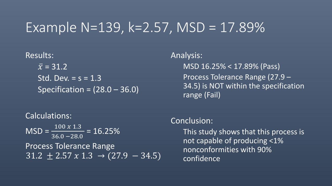
Example N=139, k=2.57, MSD = 17.89%

Results:

𝑥 = 31.2

Std. Dev. = s = 1.3

Specification = (28.0 – 36.0)

Calculations:

MSD = 100 𝑥 1.3

36.0 −28.0= 16.25%

Process Tolerance Range31.2 ± 2.57 𝑥 1.3 → (27.9 − 34.5)

Analysis:MSD 16.25% < 17.89% (Pass)

Process Tolerance Range (27.9 –34.5) is NOT within the specification range (Fail)

Conclusion: This study shows that this process is not capable of producing <1% nonconformities with 90% confidence

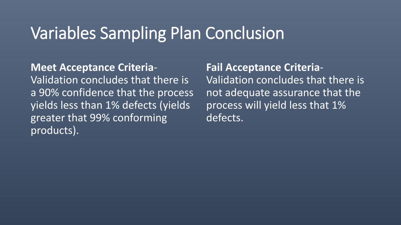
Variables Sampling Plan Conclusion

Meet Acceptance Criteria-Validation concludes that there is a 90% confidence that the process yields less than 1% defects (yields greater that 99% conforming products).

Fail Acceptance Criteria-Validation concludes that there is not adequate assurance that the process will yield less that 1% defects.

Other Sampling Plan Considerations

N Example Types Examples

1 No Variation in the system Equipment Safeties

3 No Variation in the system but want some repeatability

Vision Systems, Rejection mechanisms, Audit Trail systems

10 No Variation in the system but want a high level of repeatability

Serialization commissioning data

? Justify your sample size

Variability - Sampling is needed because processes have variability. If a process has no variability sampling can be treated differently…

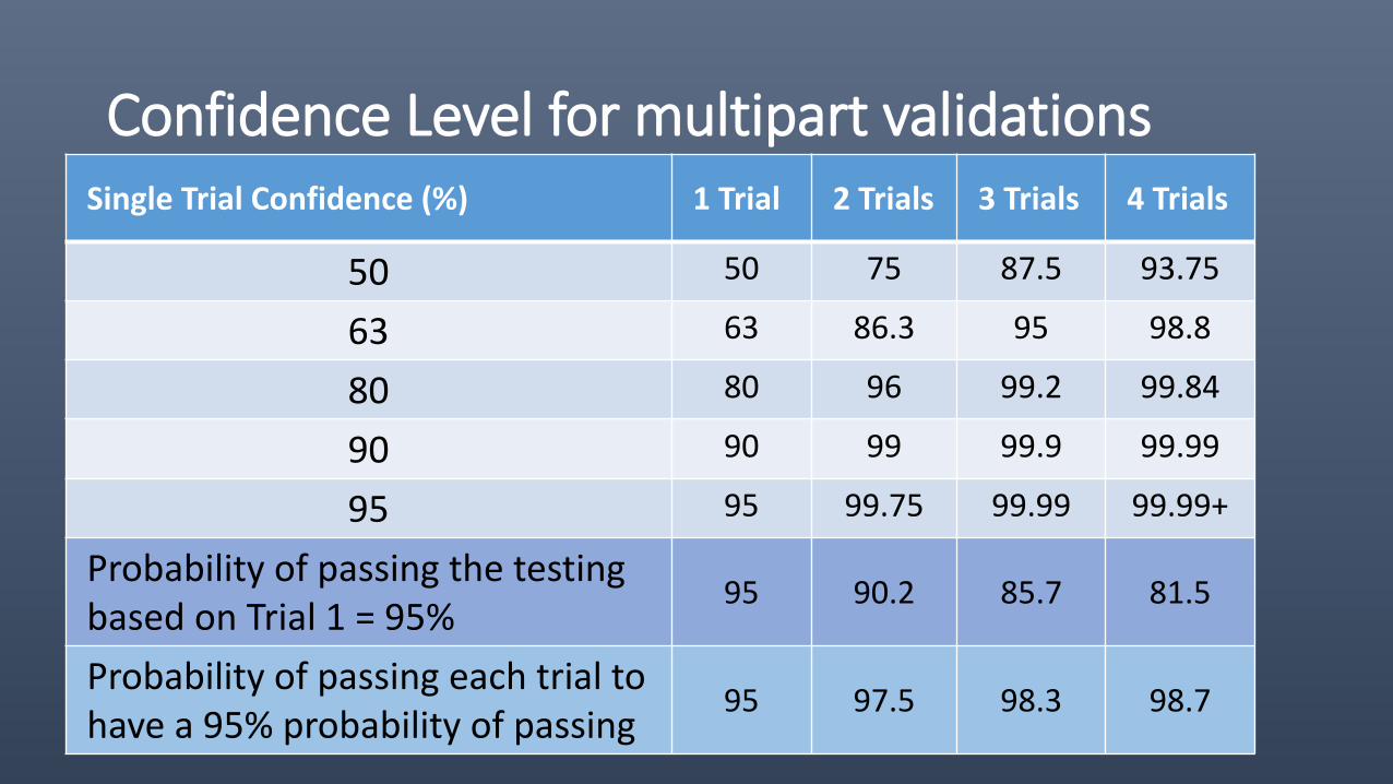
Confidence Level for multipart validationsSingle Trial Confidence (%) 1 Trial 2 Trials 3 Trials 4 Trials

50 50 75 87.5 93.75

63 63 86.3 95 98.8

80 80 96 99.2 99.84

90 90 99 99.9 99.99

95 95 99.75 99.99 99.99+

Probability of passing the testing based on Trial 1 = 95%

95 90.2 85.7 81.5

Probability of passing each trial to have a 95% probability of passing

95 97.5 98.3 98.7

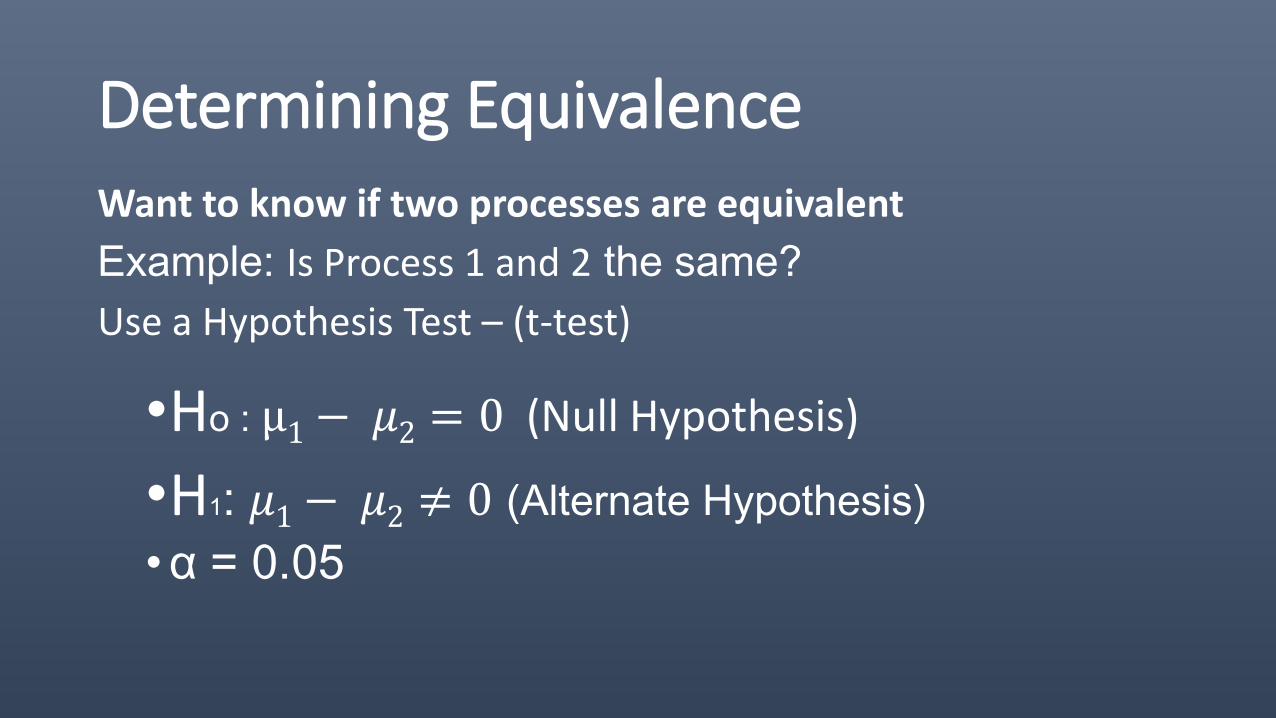
Determining EquivalenceWant to know if two processes are equivalent

Example: Is Process 1 and 2 the same?

Use a Hypothesis Test – (t-test)

•Ho : μ1− 𝜇2 = 0 (Null Hypothesis)

•H1: 𝜇1− 𝜇2 ≠ 0 (Alternate Hypothesis)

•α = 0.05

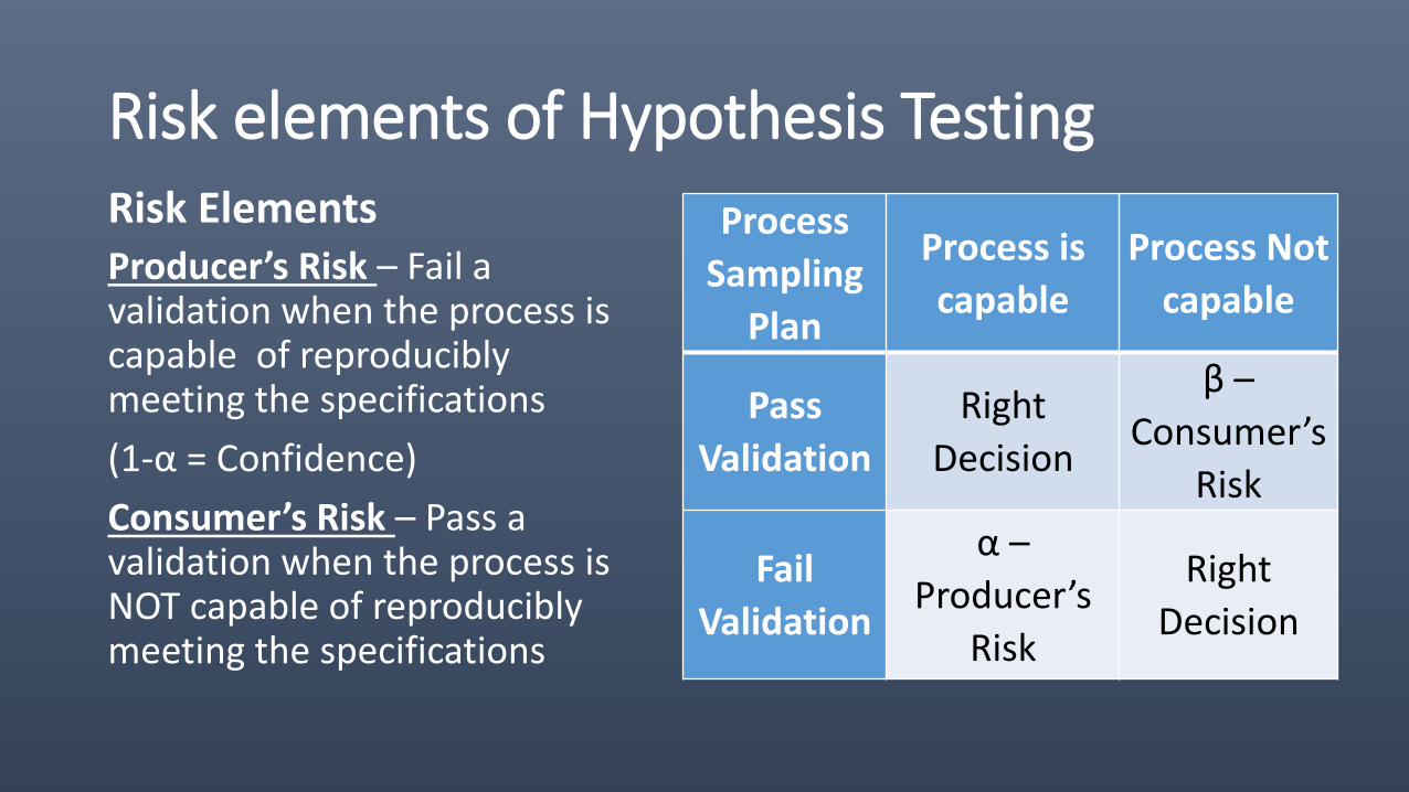
Risk elements of Hypothesis TestingRisk ElementsProducer’s Risk – Fail a validation when the process is capable of reproducibly meeting the specifications

(1-α = Confidence)

Consumer’s Risk – Pass a validation when the process is NOT capable of reproducibly meeting the specifications

Process

Sampling

Plan

Process is

capable

Process Not

capable

Pass

Validation

Right

Decision

β –

Consumer’s

Risk

Fail

Validation

α –

Producer’s

Risk

Right

Decision

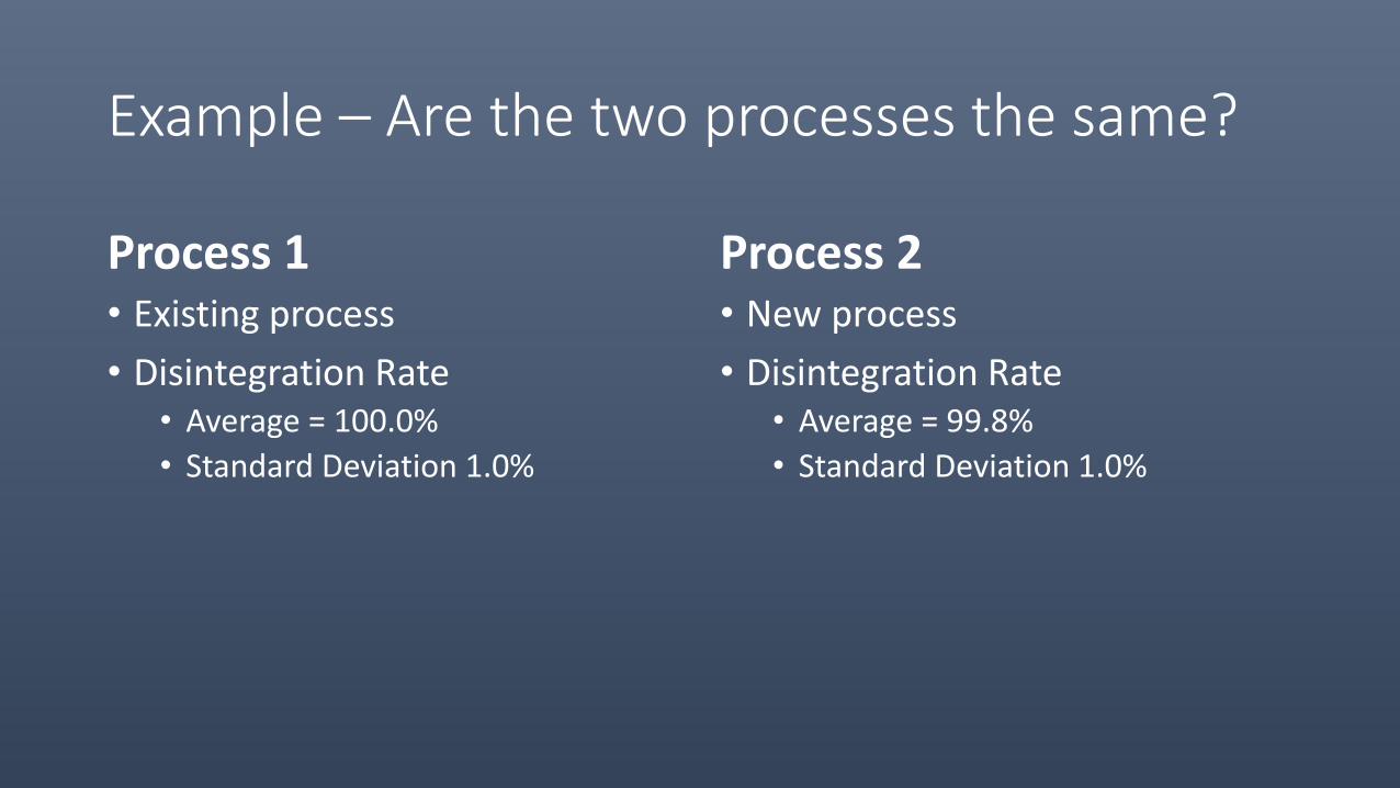
Example – Are the two processes the same?

Process 1• Existing process

• Disintegration Rate• Average = 100.0%

• Standard Deviation 1.0%

Process 2• New process

• Disintegration Rate• Average = 99.8%

• Standard Deviation 1.0%

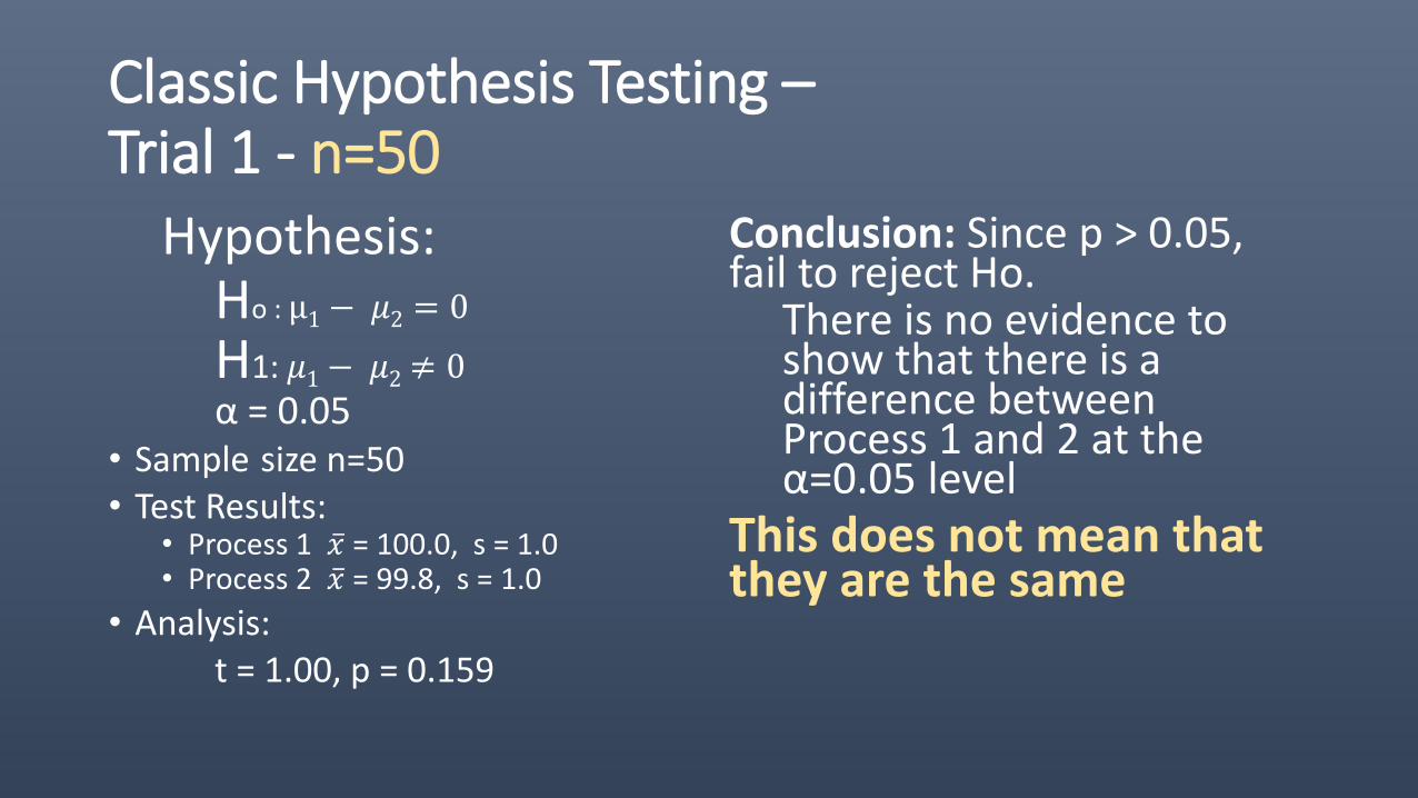
Classic Hypothesis Testing –Trial 1 - n=50

Hypothesis:Ho : μ1 − 𝜇2 = 0

H1: 𝜇1− 𝜇2 ≠ 0

α = 0.05• Sample size n=50• Test Results:

• Process 1 𝑥 = 100.0, s = 1.0• Process 2 𝑥 = 99.8, s = 1.0

• Analysis:t = 1.00, p = 0.159

Conclusion: Since p > 0.05, fail to reject Ho.

There is no evidence to show that there is a difference between Process 1 and 2 at the α=0.05 level

This does not mean that they are the same

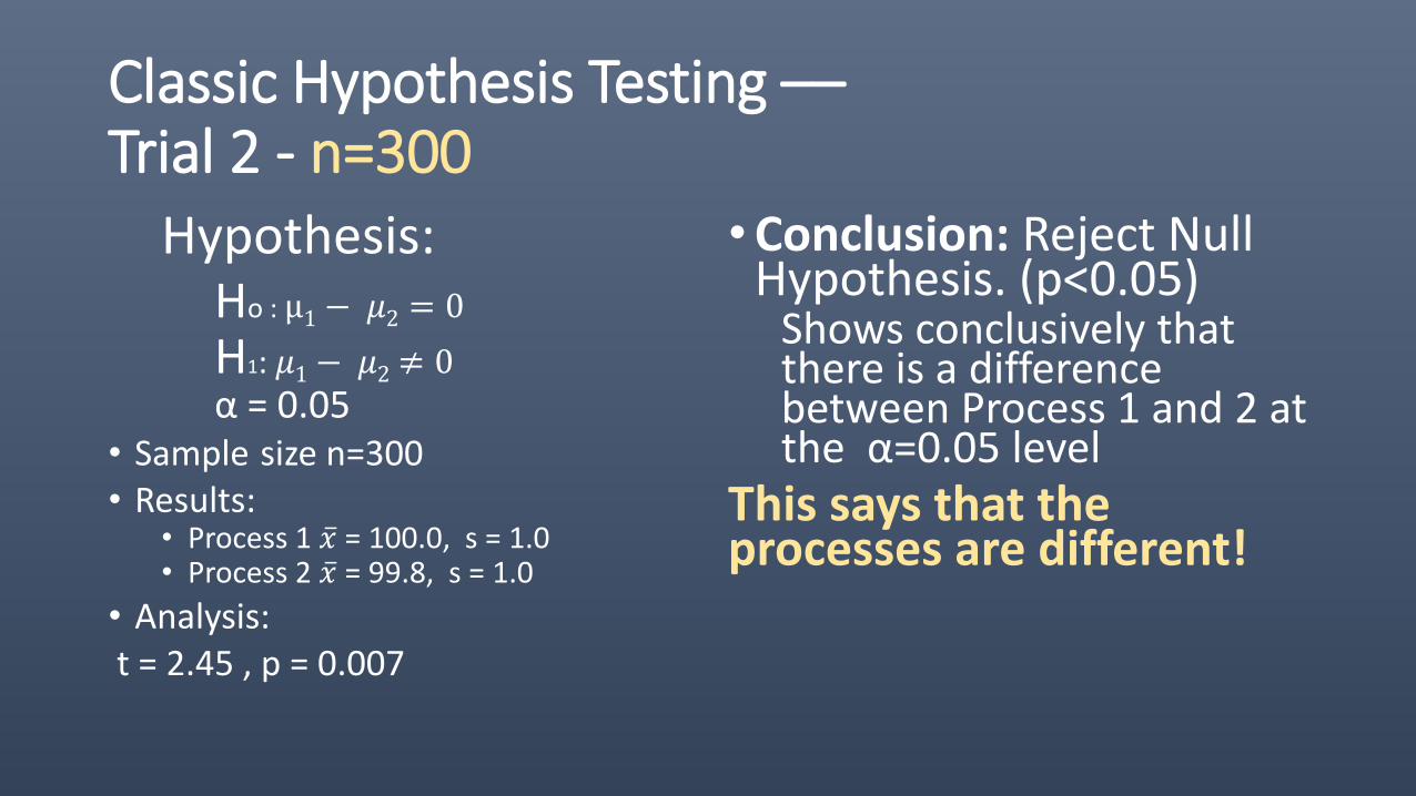
Classic Hypothesis Testing ––Trial 2 - n=300

Hypothesis:Ho : μ1− 𝜇2 = 0

H1: 𝜇1− 𝜇2 ≠ 0

α = 0.05• Sample size n=300• Results:

• Process 1 𝑥 = 100.0, s = 1.0• Process 2 𝑥 = 99.8, s = 1.0

• Analysis:t = 2.45 , p = 0.007

•Conclusion: Reject Null Hypothesis. (p<0.05)

Shows conclusively that there is a difference between Process 1 and 2 at the α=0.05 level

This says that the processes are different!

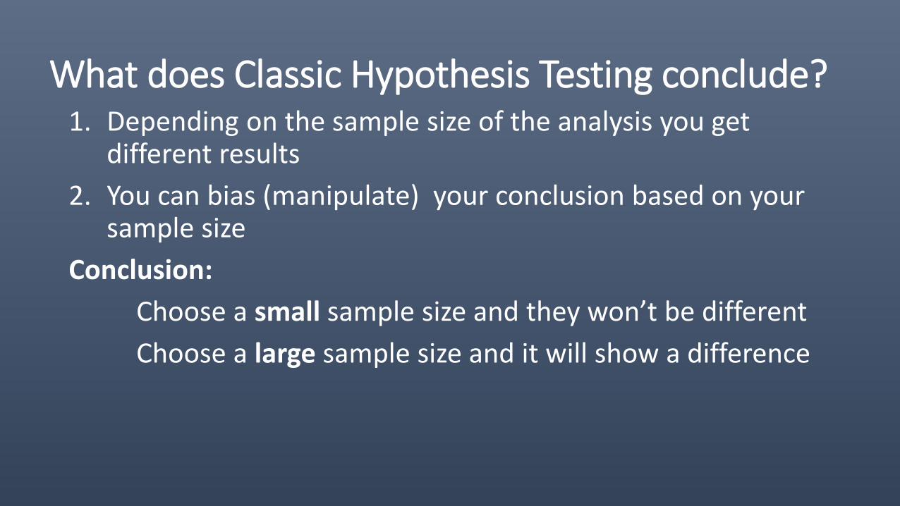
What does Classic Hypothesis Testing conclude?1. Depending on the sample size of the analysis you get

different results

2. You can bias (manipulate) your conclusion based on your sample size

Conclusion:

Choose a small sample size and they won’t be different

Choose a large sample size and it will show a difference

What have we learned?

•The Classic Hypothesis test does not show Equivalence

•Sample Size is very important the analysis

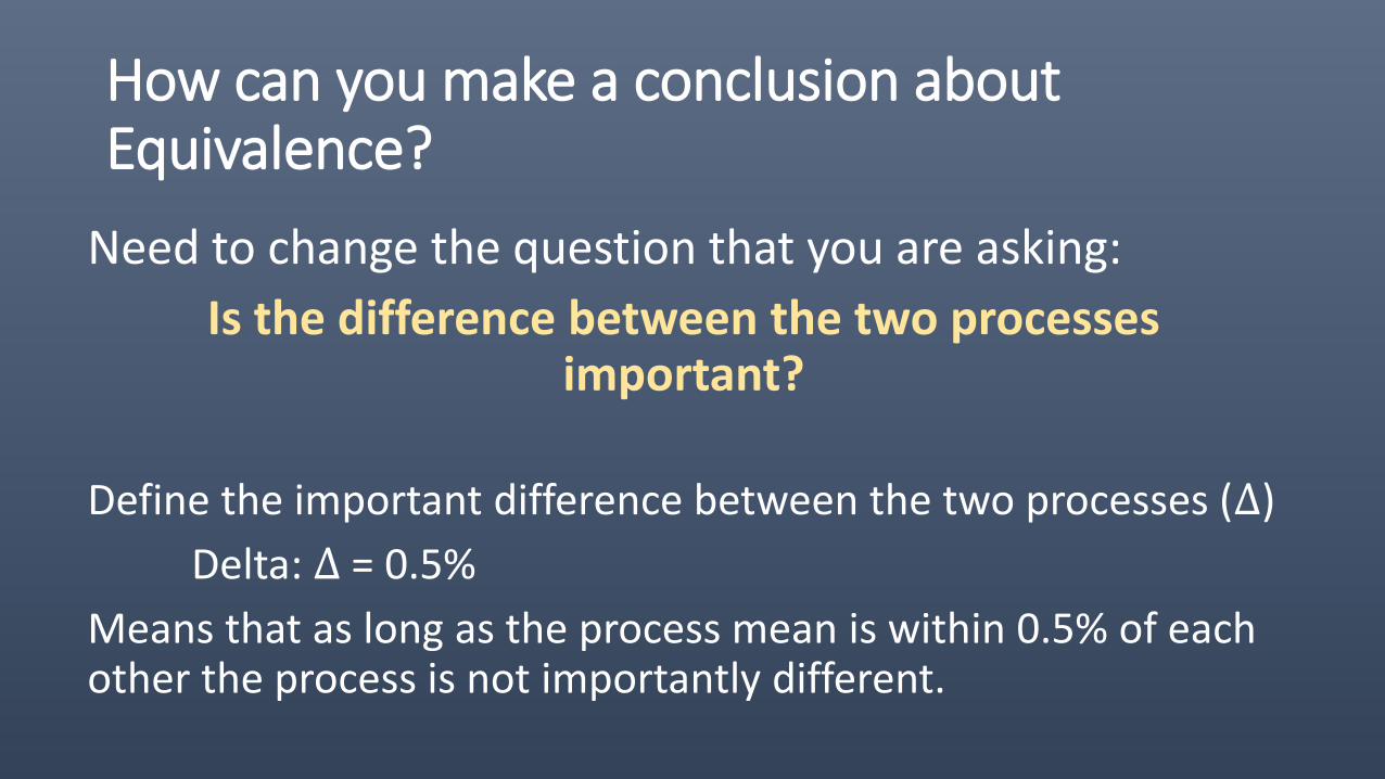
How can you make a conclusion about Equivalence?

Need to change the question that you are asking:

Is the difference between the two processes important?

Define the important difference between the two processes (∆)

Delta: ∆ = 0.5%

Means that as long as the process mean is within 0.5% of each other the process is not importantly different.

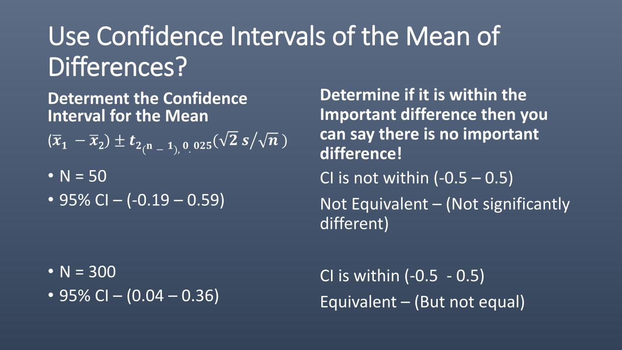
Use Confidence Intervals of the Mean of Differences?Determent the Confidence Interval for the Mean

( 𝒙𝟏 − 𝒙2) ± 𝒕𝟐(𝐧 − 𝟏), 𝟎. 𝟎𝟐𝟓( 𝟐 𝒔 𝒏 )

• N = 50

• 95% CI – (-0.19 – 0.59)

• N = 300

• 95% CI – (0.04 – 0.36)

Determine if it is within the Important difference then you can say there is no important difference!

CI is not within (-0.5 – 0.5)

Not Equivalent – (Not significantly different)

CI is within (-0.5 - 0.5)

Equivalent – (But not equal)

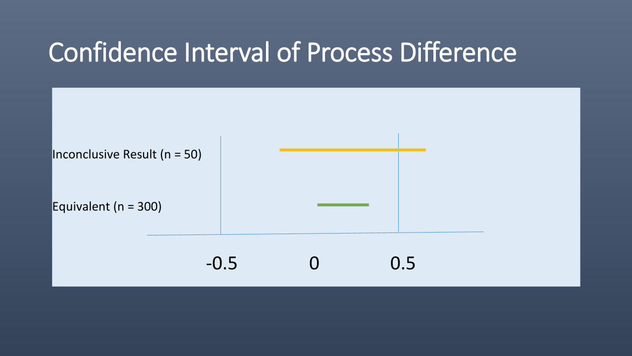
Confidence Interval of Process Difference

Inconclusive Result (n = 50)

Equivalent (n = 300)

-0.5 0 0.5

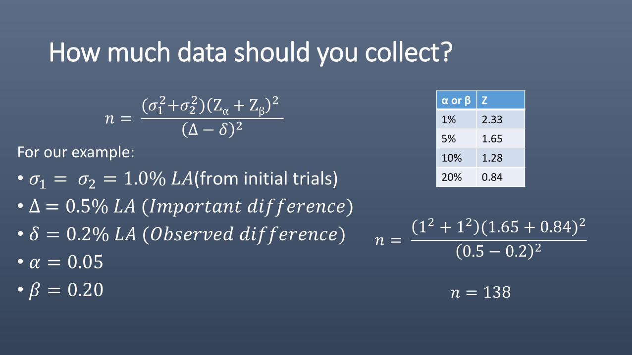
How much data should you collect?

𝑛 =(𝜎1

2+𝜎22) Zα+ Zβ

2

∆ − 𝛿 2

For our example:

• 𝜎1 = 𝜎2 = 1.0% 𝐿𝐴(from initial trials)

• ∆ = 0.5% 𝐿𝐴 (𝐼𝑚𝑝𝑜𝑟𝑡𝑎𝑛𝑡 𝑑𝑖𝑓𝑓𝑒𝑟𝑒𝑛𝑐𝑒)

• 𝛿 = 0.2% 𝐿𝐴 (𝑂𝑏𝑠𝑒𝑟𝑣𝑒𝑑 𝑑𝑖𝑓𝑓𝑒𝑟𝑒𝑛𝑐𝑒)

• 𝛼 = 0.05

• 𝛽 = 0.20

𝑛 =12 + 12 (1.65 + 0.84)2

0.5 − 0.2 2

𝑛 = 138

α or β Z

1% 2.33

5% 1.65

10% 1.28

20% 0.84

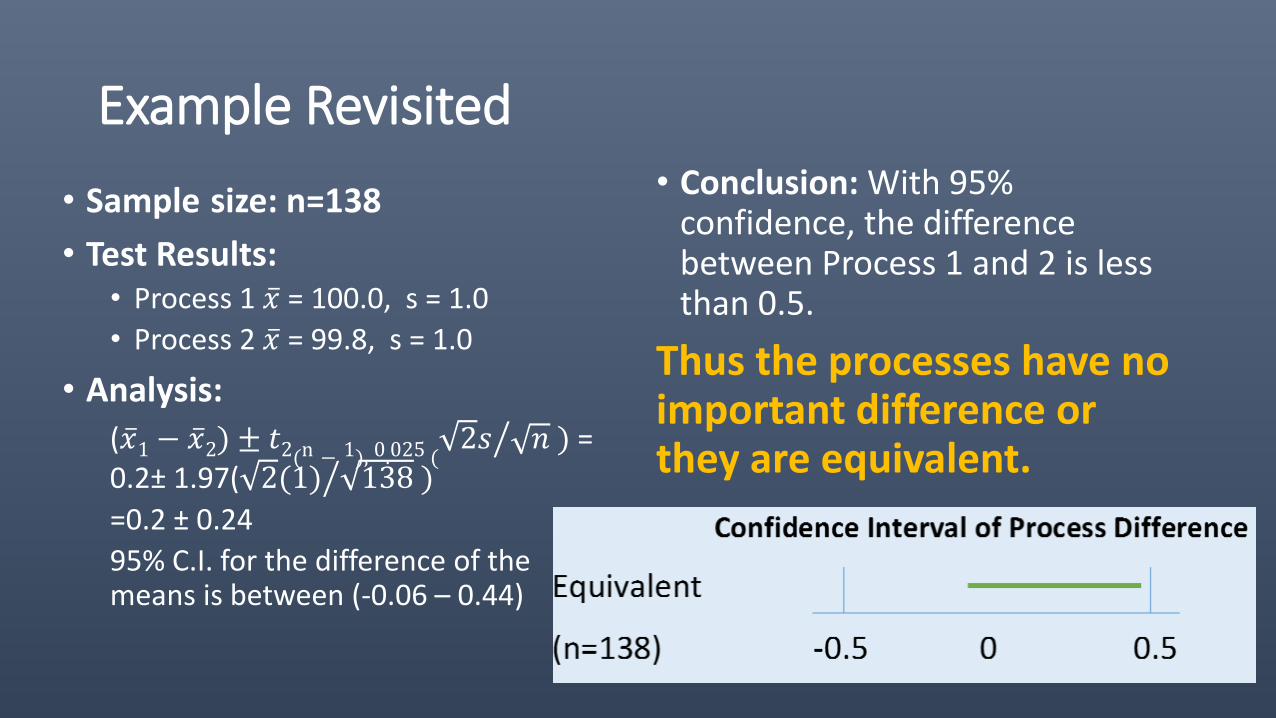
Example Revisited

• Sample size: n=138

• Test Results:• Process 1 𝑥 = 100.0, s = 1.0

• Process 2 𝑥 = 99.8, s = 1.0

• Analysis:

( 𝑥1− 𝑥2) ± 𝑡2(n − 1), 0.025 ( 2𝑠 𝑛 ) =

0.2± 1.97( 2(1) 138 )

=0.2 ± 0.24

95% C.I. for the difference of the means is between (-0.06 – 0.44)

• Conclusion: With 95% confidence, the difference between Process 1 and 2 is less than 0.5.

Thus the processes have no important difference or they are equivalent.

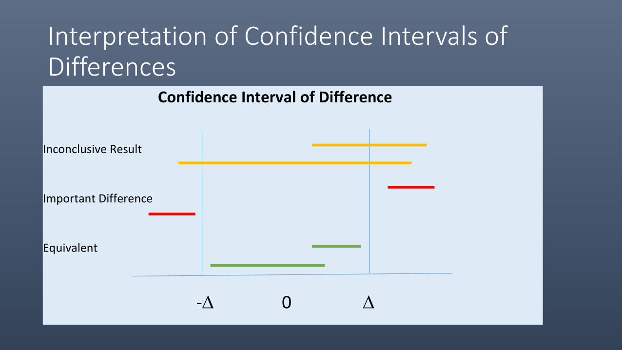
Interpretation of Confidence Intervals of Differences

Confidence Interval of Difference

Inconclusive Result

Important Difference

Equivalent

- 0

Summary

“sampling plan must result in statistical confidence”

“…samples must represent the batch under analysis.”

“…confidence level selected can be based on risk analysis ...”