SLAC - PUB - 4682 July 1988 (El

DETERMINATION OF Mz AND rz FROM THE TOTAL HADRONIC CROSS SECTION*

W. DE BOER

Max-Planck-Institut fiir Physik und Astrophysik,

Werner-Heisenberg-Institut fiir Physik, D 8000 Munich 40, Germany

and

Stanford Linear Accelerator Center

Stanford University, Stanford, California 94309, USA

ABSTRACT

We discuss the determination of the Z” mass and width from the total

hadronic cross section with emphasis on radiative corrections and normaliza-

tion errors. We find that a combined fit of the mass and width, which takes the

absolute normalization of the cross section into account, significantly reduces the

errors in these parameters in comparison to the standard procedure of fitting

only the shape of the resonance without considering the normalization. The im-

provement is especially important with small data samples; at high statistics the

methods become equivalent and independent of the size of the overall normaliza-

tion error. From a Monte Carlo study we propose a simple scanning strategy, and

also compare in detail several new Monte Carlo programs for e+e- annihilation

including higher order radiative corrections.

Submitted to Nuclear Instruments and Methods

*Work supported by the Department of Energy, contract DE-AC03-76SF00515.

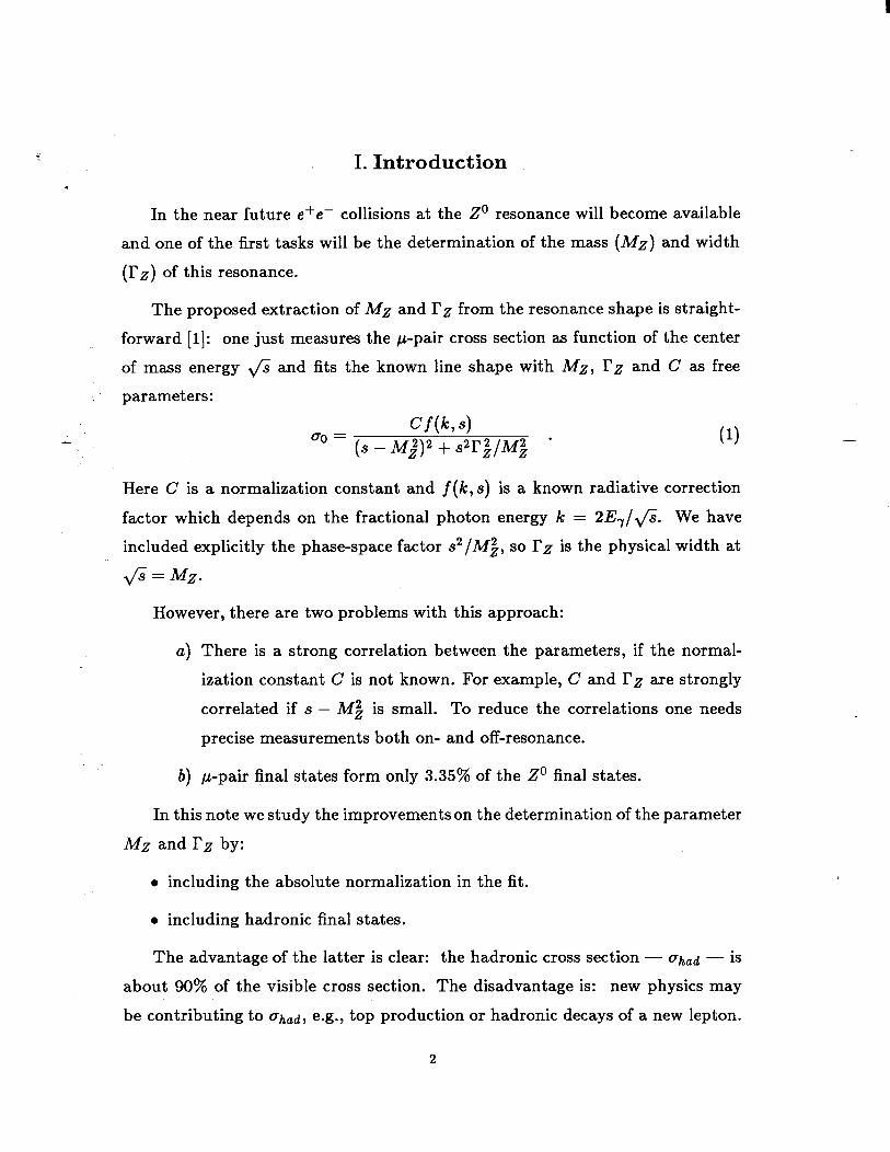
I. Introduction

In the near future e+e- collisions at the 2’ resonance will become available

and one of the first tasks will be the determination of the mass (Mz) and width

(rz) of th is resonance.

The proposed extraction of Mz and l?z from the resonance shape is straight-

forward [l] : one just measures the p-pair cross section as function of the center

of mass energy fi and fits the known line shape with Mz, I’2 and C as free

parameters:

Cf(b) uo = (s - M;)2 + 3$/M; ’ (1)

Here C is a normalization constant and j(k, ) s is a known radiative correction

factor which depends on the fractional photon energy k = 2E,/&. We have

included explicitly the phase-space factor s”/Mg, so I?z is the physical width at

@=Mz.

However, there are two problems with this approach:

a) There is a strong correlation between the parameters, if the normal-

ization constant C is not known. For example, C and rz are strongly

correlated if s - Mg is small. To reduce the correlations one needs

precise measurements both on- and off-resonance.

b) p-pair final states form only 3.35% of the Z” final states.

In this note we study the improvementson the determination of the parameter

MZ and l?z by:

l including the absolute normalization in the fit.

l including hadronic final states.

-

The advantage of the latter is clear: the hadronic cross section - ahad - is

about 90% of the visible cross section. The disadvantage is: new physics may

be contributing to f&d, e.g., top production or hadronic decays of a new lepton.

2

However, if they are contributing at a statistically significant level, it is easy to .

spot the new physics from specific decay signatures. On the other hand, if the

contribution of the new physics is too small to detect within the given statistics,

the effect on the parameters is likely to be within errors too.

Constraining the fit by the knowledge about the absolute normalization dras-

tically improves the fit stability and parameter errors. This can be understood

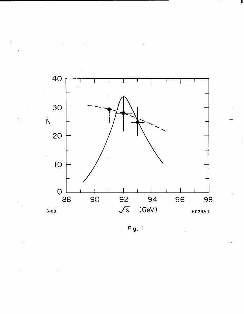
qualitatively as follows. Suppose one has only a few scan points in the neigh-

borhood of the resonance (see fig. 1). If the errors are large, the shape is not

well-determined. For example, the dotted line would be an acceptable fit, if only

the shape is fitted. However, such a large width would give a too low absolute

peak cross section, since this varies quadratically with the total width.

In sec. V we will compare quantitatively two fitting methods:

l A three-parameter fit of C, Mz and l?z to the shape of the resonance. In

this case one only needs to measure the relative luminosity of the different

scan points.

l If one assumes the constant C to be known from the Standard Model, one

needs only a two-parameter fit of Mz and I?z to the absolute cross section,

measured as function of center-of-mass energy. In this case one has to

measure the absolute normalization of the scan points. C depends only on

the coupling constants between the 2’ and fermions, which are known to

agree very well with the Standard Model predictions [2]. The systematic

uncertainties from the luminosity monitor and the Monte Carlo acceptance

corrections can cause a correlation between the different scan points. The

effect of such correlations turns out to be small as will be discussed in detail.

To get the resonance shape and the absolute normalization correct, radiative

corrections have to be applied. Since these corrections are sizeable, one has to

include higher orders too. We have made a detailed comparison of several new

Monte Carlo generators for p-pair production, which include the higher-order

corrections.

3

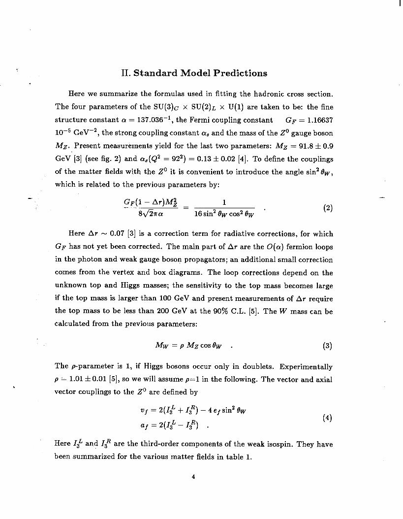
II. Standard Model Predictions

Here we summarize the formulas used in fitting the hadronic cross section.

The four parameters of the SU(3)c x SU(2)h x U(1) are taken to be: the fine

structure constant CII = 137.036-l, the Fermi coupling constant GF = 1.16637

10m5 GeV2, th e s t rong coupling constant cyB and the mass of the Z” gauge boson

Mz. Present measurements yield for the last two parameters: Mz = 91.8 f 0.9

GeV [3] (see fig. 2) and cr,(Q2 = 922) = 0.13 f 0.02 [4]. To define the couplings

of the matter fields with the 2’ it is convenient to introduce the angle sin2 0w,

which is related to the previous parameters by: -

GF(~ - Ar)Mi = 1 8&o 16 sin2 8~ cos2 8~ ’ (2)

Here Ar - 0.07 [3] is a correction term for radiative corrections, for which

GF has not yet been corrected. The main part of Ar are the O(a) fermion loops

in the photon and weak gauge boson propagators; an additional small correction

comes from the vertex and box diagrams. The loop corrections depend on the

unknown top and Higgs masses; the sensitivity to the top mass becomes large

if the top mass is larger than 100 GeV and present measurements of Ar require

the top mass to be less than 200 GeV at the 90% C.L. [5]. The W mass can be

calculated from the previous parameters:

Mw = p MzcosOw . (3)

.

The p-parameter is 1, if Higgs bosons occur only in doublets. Experimentally

p = 1.01f0.01 [5], so we will assume p=l in the following. The vector and axial

vector couplings to the Z” are defined by

vf = 2(13L + IzR) - 4ef sin2 8~

af = 2(IzL - 13R) . (4

Here TaL and 13R are the third-order components of the weak isospin. They have

been summarized for the various matter fields in table 1.

4

i

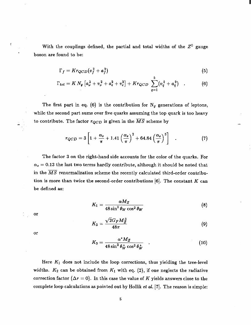
. With the couplings defined, the partial and total widths of the Z” gauge

boson are found to be:

I-f = Kr@& + u;, (5) I’tot = K N, [a; + v,” + a; + $1 + K~QCD f&? + a,“) . (6)

q=l

The first part in eq. (6) is the contribution for N, generations of leptons,

while the second part sums over five quarks assuming the top quark is too heavy

to contribute. The factor rQCD is given in the MS scheme by

l+ % f1.41 2

+ 64.84 a, 3 ( )I .

7r

The factor 3 on the right-hand side accounts for the color of the quarks. For

o8 = 0.13 the last two terms hardly contribute, although it

in the MS renormalization scheme the recently calculated

tion is more than twice the second-order contributions [6].

be defined as:

or

Kl = aMZ 48 sin2 9~ cos2 8~

or

K 2

= JZCFM,”

48~

K3 = a*Mz

48 sin2 0$ cos2 8 * ’ W

should be noted that

third-order contribu-

The constant K can

(8)

(9)

(10)

Here Kl does not include the loop corrections, thus yielding the tree-level

widths. K2 can be obtained from K1 with eq. (2), if one neglects the radiative

correction factor (Ar = 0). In this case the value of K yields answers close to the

complete loop calculations as pointed out by Hollik et al. [ 71. The reason is simple:

5

i GF was calculated from muon decay without radiative corrections from the W-

. exchange graph, so GF includes these corrections. Since the loop corrections for

W- and Z”-exchange are similar, just using K2 in calculating the width yields

answers very close to the exact answer. K3 uses the running couplings where

all loop corrections are absorbed in the Q2-dependent coupling constants. The

“starred” (= running) couplings were calculated by Lynn et al. [8] by summing

the loop corrections to all orders. At low energies K3 = Kl, while at the Z”

energies K3 - K2.

From eqs. (5) and (6) it is clear that the branching ratios I’f/I’tot are indepen-

dent of the parameterization of K and they are completely specified once sin2 8~

is known and the number of generations is known. For the world average [2-51

of sin2 8~ = 0.230 f 0.005 one finds for three generations (and excluding the top

quark contribution) :

be - = 3.35 f 0.01% rtot

r - +j65+ O-04g YlJ hot

. - 0.03 O

Jk = 70.00 f 0.12% hot

.

The total hadronic cross section is given by:

q=l

a7z _ ~-!*K~QcD GXqVeVq

q=l had -

Mz (s - M;)2 + s21&/M;

z _ 127FrQCD sK2(v,2+u,2) e(v,z +a;)

Ohad - q=l

M; (s - Mg)2 + s”I’;ot/M; ’

(11)

(13)

w4

WC)

6

i The

. and

superscripts indicate the contribution from photon exchange, Z” exchange

their interference and K is one of the K’s defined in eqs. (8)-(10). The

sum is taken over five quark flavors, thus assuming the top quark is too heavy.

Combining eqs. (5) and (14~) one finds the important result that on resonance,

when s = Mj,

peak _ l2 7r reerqq Ohad --

M; rtzot (15)

is independent of K and thus largely independent of uncertainties in the loop

corrections coming from the unknown top and Higgs masses.

Choice of K-factor

The parameters describing the total cross section in eq. (14) are: cy, 08,

Mz, rz, eet eq,ve, vq, a, uq and, in addition, GF or sin2 8w depending on the

choice of K-factor [eqs. (S)-(lo)]. Th e most unknown and most interesting pa-

rameters are Mz and I’z, so one can try to optimize the knowledge on these

parameters by taking the other parameter values from independent processes.

For example, Q, ee, eq, a, and uq are well-known; ve and vq are reasonably well-

known from eq. (4) and the world average of sin2 Bw and the uncertainty of 0.02

in CY$ yields an uncertainty in the peak cross section of 0.4% only. The remaining

choice to be made is the K-factor. Experimentally, K2 is most accurately known

and therefore preferred. Furthermore, by using K2 the radiative corrections are

smaller and easier to handle. First of all, because the width calculated with K2 is

very close to the width calculated with the complete radiative corrections. There-

fore, the shape is correctly described and the initial-state radiative corrections,

which are rather sensitive to the shape, can be calculated in a straightforward

way. Secondly, the electroweak loop corrections are small, if one uses K2, since

K2 and K3 are almost identical in the 2’ resonance region.

If one uses K3 or Kl instead of K2, one can in principle fit sin2 8w as an

additional free parameter [the dependence of the cross section on this parameter

is now much stronger than the dependence via the vector couplings alone as

7

‘

g iven by e q . (4)]. 0 n e c a n th e n m a k e a test o f th e S ta n d a r d M o d e l by c o m p a r i n g . th is va lue o f s in2 B w wi th th e wor ld a v e r a g e . A n a l ternat ive test w o u l d b e to

d e te r m i n e Mz us ing K 2 , inser t its va lue in to e q . (2) a n d c o m p a r e th e left- a n d

r igh t -hand s ides in e q . (2) . H o w e v e r , th e s e tests a re m o d e l - d e p e n d e n t in th e s e n s e

th a t th e y d e p e n d o n th e u n k n o w n to p a n d H iggs m a s s e s : in case o f K l o n e h a s

to app ly th e rad ia t ive cor rect ions to th e d a ta , in case o f K 3 o n e h a s to ca lcu la te

K 3 fo r a cer ta in to p a n d H iggs m a s s a n d in case o f K 2 o n e h a s to ca lcu la te A r

in e q . (2). In th e fits desc r ibed in sec. V w e h a v e u s e d th e p a r a m e tr izat ion wi th

: G F (K2) .

- T h e to ta l c ross sect ion

F r o m e q s . (ll), (13 ) a n d (15) th e had ron i c p e a k cross sect ion is fo u n d to

b e 4 0 .7 n b a t th e B o r n level . T h e obse rvab le p e a k cross sect ion a fte r rad ia t ive

cor rect ions is 0 .7 3 6 x 4 0 .7 = 3 0 .0 n b (see n e x t sect ion). Th is c ross sect ion de -

p e n d s q u a d r a tical ly o n th e to ta l w id th a n d is th e r e fo re sensi t ive to th e n u m b e r

o f n e u tr ino spec ies wi th m a s s e s less’th a n hal f th e Z” m a s s . If o n e exp resses Ice

a n d Iq q as f ract ions o f th e to ta l w id th [see e q s . (11) a n d (13)], o n e fin d s fo r th e

c o n tr ibut ion o f N F e w n e w n e u tr inos:

g ”,“B ” - l2 7 r ( 0 .0 3 3 5 ) ( 0 .7 0 0 ) - ? @ (1 + 0 .0 6 6 5 N y n e w ) 2 ’

O n e n e w n e u tr ino g e n e r a tio n wi l l l ower th e p e a k cross sect ion by 1 2 .7 % inde -

p e n d e n t o f m t a n d m H a n d th is shou ld n o t b e to o diff icult to d e tect: wi th a 5 %

statist ical e r ror (imp ly ing 4 0 0 obse rved 2 ’ e v e n ts) a n d a 5 % systemat ic uncer -

tainty, th e one -s i ded 9 0 % C . L . l ower lim it w o u l d b e 1 1 .5 % , wh ich is still b e l o w

th e c h a n g e e x p e c te d fo r o n e n e w n e u tr ino g e n e r a tio n . H e r e w e a s s u m e d th a t th e

m a s s o f th e n e w n e u tr ino is a t least a fe w G e V b e l o w hal f th e Z” m a s s . M o r e

q u a n tita t ive resul ts o n th e to ta l e r ror o f Ito t wi l l b e g i ven in sec. V .

i III. Radiative Corrections

In order to measure either the shape or the absolute cross section, one has

to apply radiative corrections. For hadronic final states these reduce to

l Initial state radiation from the electrons. Final-state electromagnetic radi-

ation from the quarks is small since

a) The Kinoshito-Lee-Nauenberg theorem assures that the procedure of

summing over all qij final states with an arbitrary number of photons, as

is done in the detection of multihadronic events, will cancel all leading

logarithms and the remaining radiative correction is of order 0 (f) M

0.2%.

b) Fragmentation of quarks (strong interactions) is fast compared to the

timescale of electromagnetic radiation.

l Loop corrections to the gauge boson propagators, which are called vacuum

polarization corrections in case of the photon and “oblique” corrections

in case of the weak gauge bosons. These loops depend on the maximum

Q2 of the gauge boson and can be taken into account by either modifying

the coupling constants (“running” coupling constants) or by correcting the

propagators. The size of the loop corrections depends strongly on energy:

at s = Mi the effect is small, since the K-factors largely cancel out [see

eq. (15)]. Off- resonance, where (s - Mj)2 > MiTg, the radiative cor-

rections are Ki/K 12. This factor is approximately 1.14 at fi = 80 GeV,

where 12.6% comes from the running of cx and the remaining part comes

from vertex and box diagrams.

The size of initial state radiative corrections is shown in table 2; the factors

were calculated with different Monte Carlo generators and from the formulas

of ref. [9] with the program ZAPPR from G. Burgers. The Born cross section

has to be multiplied by these factors in order to obtain the corrected cross sec-

tion. The minimum allowed invariant mass squared of the final state - sl -

9

i was taken to be 1% of s in all calculations. It can -be seen that the first-order . corrections change the Born cross sections by factors between 1.9 and 0.7; for

such large corrections the higher-order corrections are important. Until recently

these higher-order corrections had been estimated by an approximate procedure,

called “exponentiation;” recently Berends, Burgers and van Neerven [9] showed

that these estimates are very close to the exact second-order calculation. Several

new Monte Carlo generators have become available, which include higher-order,

initial-state radiative corrections as well as the loop corrections. An overview is

given in table 3. The ones of interest to hadron production are:

l MMGE. This is the original Berends-Kleiss-Jadach [lo] p-pair generator

updated by J. Alexander (11) with the second order calculations of ref. [9].

The program has various options:

Calculate first- (second-) order initial-state radiation with at most one

(two) photon(s) from initial-state radiation.

Exponentiate the cross sections to include the effects of multiple soft

photon emissions (both first and second order). The program does not

include the loop corrections.

l YFS. This program from Jadach and Ward [12] follows the exponentiation

procedure from Yennie, Frautschi and Suura [ 131. It is unique in the sense

that it calculates higher-order initial state radiation with multiple photons

generated as real particles, thus taking correctly the kinematics of multiple

photons into account including a non-zero invariant mass. In the previous

program MMGE only the remaining energy after radiation was calculated

and the missing energy was attributed to a single effective, massless photon.

l EXPOSTAR. This program, developed by Im, Kennedy, Lynn and Stu-

art [S], takes all the loop corrections into account by calculating the run-

ning couplings. Higher-order, initial-state radiative corrections are taken

into account via the structure function approach [14], in which the lon-

gitudinal momenta of the electron or positron are partially transferred

-

10

. to photons. Since. these photons cannot have transverse momenta, the

program is not suitable as a Monte Carlo generator, but it is very useful

to check total cross sections and radiative correction factors. In the pro-

gram BREMG these transverse components will be reinstated by combining

the original Berend-Kleiss-Jadach generator (BREM5) with EXPOSTAR.

However, BREMG has not yet been released.

Figure 3 shows the effect of higher-order contributions to the differential

cross section da/dv. Here v = 1 - s’/s, where s and s’ are the invariant masses

squared of the initial and final state, respectively. In first order v would just be

the fractional photon energy Er/Ebeam. In second order one cannot speak about

the photon energy, but s’ is still a well-defined quantity. One observes that higher

order contributions shift the events towards larger v, as expected since larger v

corresponds to smaller s’ and more initial state radiation reduces s’.

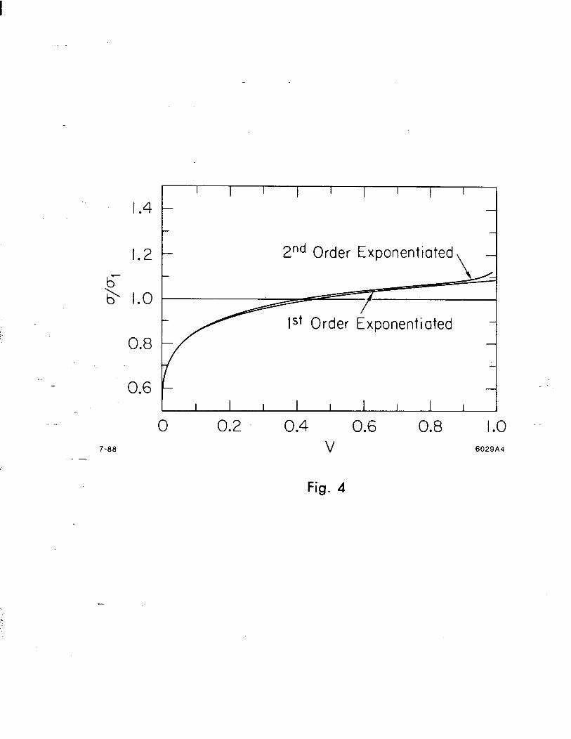
Figure 4 shows the ratio between the second order and first order differential

cross section. One observes a large decrease (20-30010) in the region of soft real

photons (v + 0), which is only partially compensated by an increase of approxi-

mately 10% in the region of hard photon radiation (large v). The fact that the

total cross section still increases by 0.8% is due to the increase in the infrared

part of the cross section.

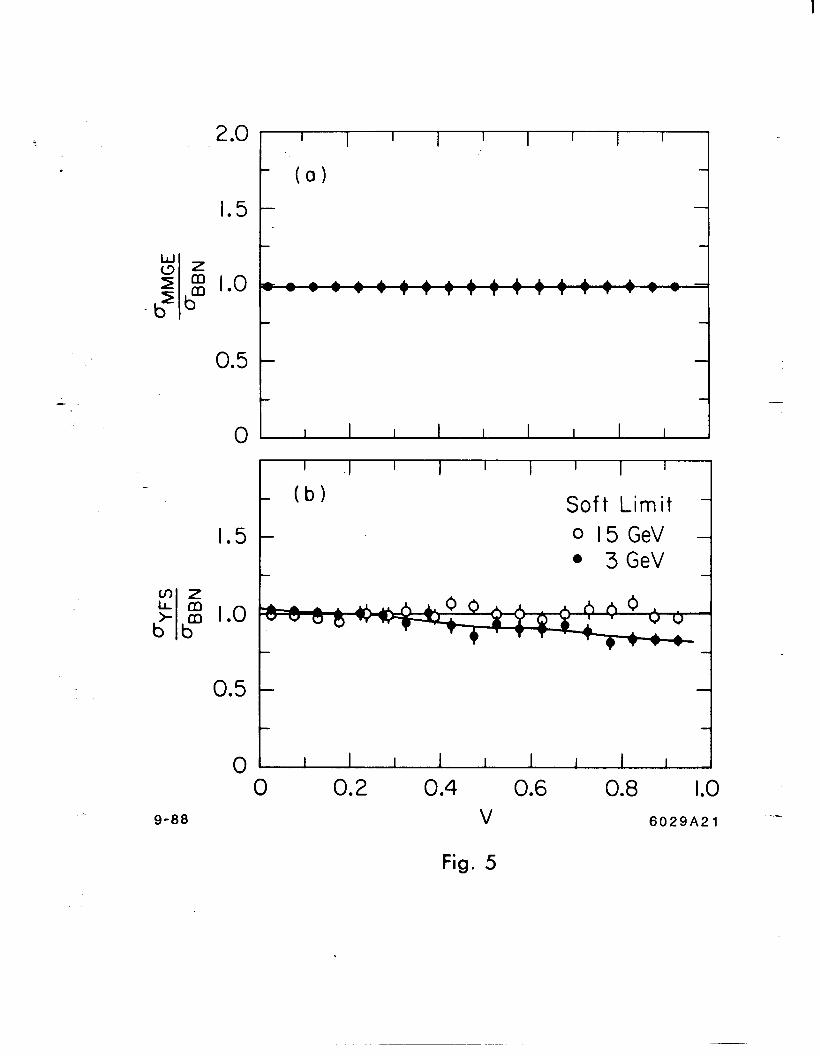
In fig. 5 we compare the differential distributions da/dv for the MMGE and

YFS Monte Carlo generator with the analytical formula of ref. [9] by plotting the

Monte Carlo events and weighting each entry with the inverse of the analytical

formula, so one expects a straight line close to 1.

One sees that both programs agree well with the analytical formulae. For

- YFS we plotted the results for two values of the maximum allowed energy of the

photons, which can be radiated in addition to the first photon. One sees that

the contribution from two or more hard photons is appreciable.

11

i

. At energies above -the Z” mass both the YFS cand MMGE programs deviate

appreciably from the results of the EXPOSTAR program. This is due to the fact

that the latter program includes the loop corrections, which cause a larger width

of the resonance (EXPOSTAR calculates the width with K3, while the other

programs use Kl). Simply inserting a larger width in the other programs will

make the radiative correction factors to become similar, but then the peak cross

section will be wrong. One has to include correctly the running of the coupling

constants, since even approximating K3 with K2 does not yield the correct answer

as seen from the comparison of f$&, and f2Ki in table 2, although the difference

is less than 1%. -

In table 2 we have also included a column with the total cross section for

p-pair production after all radiative corrections. The cross section for the other

channels can be calculated from the relative branching ratios [see eqs. (ll)-(13)]

and the relative contributions of photon and 2’ exchange [see eq. (14)]. The

absolute cross section in table 2 is in good agreement with the result calculated

from the experimental branching ratios [eqs. (ll)-(13)] only if we apply the weak

vertex corrections consistently to both the running coupling constants in eq. (14)

and the width. This was not done in EXPOSTAR and ref. [8], so the peak cross

section is lower in that case by about 20 pb compared to the value in table 2,

but is closer to a recent calculation by G. Burgers [15] (10 pb lower).

IV. Fitting Method for Correlated Errors

The best estimates of Mz and I’z can be extracted from the data via a fitting

procedure, e.g., minimizing the x2 [16]. Correlated errors between measurements

can be taken into account in one of the following ways [17]:

a) Define the x2 via an error correlation matrix:

x2=ATV-rA . (17)

-

12

Here A- is a column vector containing the residuals between measure-

ments (R;) and fitted values (Rfit) and V is the error correlation ma-

trix:

Ai = Ri- Rfit

Vii = E(Ri - Rfit)2 = CJ; + a;

Vij = E(Ri - Rfit)(Rj - Rfit) = a; .

(18)

E indicates that the expectation value has to be calculated, ai is the

error on R; and on is the overall normalization error, which indicates

how far the observed value(Ri) can deviate from the true value (Rt),

soRi=Rt f on. This last expression inserted in the expectation

values in eq. (18) yields the results for the elements of V. Note that C$

is the variance of Rt, so it contains the uncorrelated part of the error,

which includes both the statistical error and point-to-point system-

atic error, but excludes’the overall normalization error. For example,

for two measurements R1 and R2 with statistical errors of 10% and a

normalization error of 5%, the matrix is:

v= (0.1 RI)~ + (0.05 RI)~ (0.05 R1R2)2

(0.05 R1R2)2 (0.1 R2)2 + (0.05 Rz)~ ’

The following points are worthwhile noting:

l This error matrix is N x N for N data points and should not be confused

with the M x M error matrix for M fitted parameters: the first matrix is -

input to the fit program, the second one output.

l The importance of systematic errors can be studied by varying the off-

diagonal elements and observing the influence on the fitted parameters.

13

b) A second method commonly used to take correlated errors into account

is the following: Define a likelihood function by multiplying the proba-

bility of each data point with the common probability factor from the

overall normalization factor f, which is assumed to have a Gaussian

distribution with mean 1 and r.m.s. on:

L = 5 ,-(gy’,-qq . (19) i=l

For small event samples the Gaussian event error distribution can be

replaced by a Poisson distribution.

One can optimize the likelihood by minimizing

(fRi - RfitJ2 w-3)” -

(20)

f can either be treated as a free parameter or one integrates over all

possible f values in the fit.

Methods a) and b) usually give similar results. However, the first method

.-- -is more flexible in the sense that it defines a correlation between every pair of

data points and it does not require a specific error probability distribution as is

needed in case of the maximum likelihood approach. Therefore we will use the

first method.

14

V.-Monte Carlo Fit Results

Before generating MC events one has to decide the number of scan points and

the distance A between the scan points. To fit eq. (1) to the shape, one needs

at least three scan points. If one measures the averaged energy for each event,

one could have as many energy points as events. This can be easily included in

the fit of the data as a function of energy, but for the moment we will assume

that we have the equivalent of three data points at three energies separated by a

distance A. Data point at more energies can only improve the fit, so the results

present a pessimistic limit.

Since the mass of the 2’ is not known accurately, one may miss the peak by

some amount. We therefore generated Monte Carlo events in three energy bins

each A GeV apart and assumed the central point misses the peak by E GeV, so

E=<&>-MZ.

We generated the events first as function of E for different values of A, then

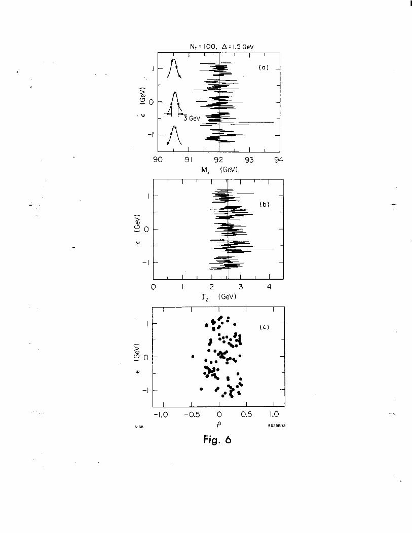
as function of A for different values of c. Figures 6 and 7 show some typical fit

results for Mz and l?z as function of E for A = 1.5 and 1 GeV, respectively. Each

error bar corresponds to a fit for a total luminosity of 3.3 nb-l divided equally

over three scan points. If the points were centered around the peak, i.e., E = 0,

this corresponds approximately to

33 events at 92 GeV,

25 events at 93 GeV, and

22 events at 91 GeV.

One sees from figs. 6 and 7 that the fitted values of Mz and I’z cluster

around the generated values of 92 and 2.55 GeV, respectively, even if E = fl .-

GeV. For these values of E and A = 1 GeV one measures only on one side of the

resonance (see the insets in figs. 6a and 7a for scan point positions for E = 1, 0,

and -1 GeV). In this case the correlation between Mz and I’z becomes large as

shown in fig. 7c, top and bottom. As soon as one measures on both sides of the

peak, the correlation becomes reasonably small even if E = flGeV (see fig. 6~).

15

i Typical errors are 200-350 MeV, both for Mz and.-I’z. Here we assumed that

. the luminosity was measured with a total systematic uncertainty of 15010, which

we assumed to be fully correlated between the data points. The statistical error

on the luminosity was assumed to be small compared with the systematic error

and therefore neglected. The effect of larger systematic errors will be discussed

hereafter.

Figures 8 to 10 show the typical error on Mz and l?z as function of the scan

range (defined as 2A) for E = 0, 0.5, and 1 GeV, respectively. The two lower

curves show the correlations between Mz and l?z and the number of events

- normalized to the total number of “peak” events Nt, where Nt is the number

of events expected if all the luminosity was taken at the peak of the resonance.

This ratio decreases if the scan range increases since the luminosity was kept

constant. The different symbols correspond to different values of “peak” events.

If one measures symmetrically around the peak (E = 0, fig. 8), the correlation p is

small and the smallest errors are obtained for a small scan range, thus optimizing

the number of events. If the central point misses the peak by 0.5 or 1.0 GeV the

smallest error in Mz is obtained for a larger scan range (see figs. 9 and lo), while

the smallest error in I’z is obtained for the scan range optimizing the number of

events.

Figure 11 shows the dependence of the expected error in I’z on the scan range

for different mixtures of statistical and normalization errors. One sees that for a

luminosity corresponding to 100 “peak” events the results from a two parameter

fit (Mz and I’z) gives a considerably better result than a three parameter shape

fit in which the the normalization constant is an additional free parameter. This

holds even for very large statistics (10’ Z”‘s) and large normalization errors;

the two parameter fit results shown have normalization errors of 3, 15 and 25%,

respectively.

With high statistics and a sufficiently large scan range all fits become similar

and independent of the normalization error (see fig. 11, top curve). The reason is

16

simple: Mz is best d t e ermined by points on the steeper slope of the resonance,

while I’z is most sensitive to the peak cross section, where the term (s - Mi)

is small. One cannot determine one parameter precisely without knowing the

other, so one needs a certain minimum scan range and the most unbiased way

of extracting Mz and I’z is a simultaneous fit of both parameters. If the scan

range is large enough, the normalization error can move all points up and down,

but this does not change the shape. In this case the shape fit and the fit of the

absolute cross section become equivalent. Note that the final error on the width

is determined by the point to point systematic uncertainties, which we assumed

to be 1% for the curves in fig. 11. Even with lo2 to lo3 events one can get useful

limits on the number of generations with light neutrinos (masses less than M,7/2),

since the errors on the total width become comparable to the contribution of a

new neutrino generation, which is shown as a dashed horizontal line in fig. 11.

VI. Scanning Strategy

We assume the first data will be taken at a center-of-mass energy close to the

expected Z” mass of 92 GeV (see fig. 2). If one takes 1 nb-l (SZ 30 “peak” events)

and assumes the width to be equal to the predicted value of 2.55 GeV, one can

calculate from eq. (14~) the relative position of the peak, namely (s - Mi)2. The

accuracy of the peak position is about 0.4-0.7 GeV, depending on how far one

misses the peak (see horizontal error bars in fig. 1). The error becomes larger at

the peak, since the cross section is rather flat near the peak. In the unlikely case

that one misses the peak by several GeV, the best strategy would be to-find the _- peak and one should change the energy by the amount given by the measured

s-M;.

Because of the quadratic ambiguity in (s - Mi)2, one does not know in which

direction to move. We propose to move up in energy, since this has the advantage

of the larger cross section from the radiative tail. We will not consider any further

17

the pessimistic scenario of missing the peak by several GeV, since this has been

- worked out before [18].

If one misses the peak by 1 GeV or less, one can see from figs. 8-10 that a

reasonable scan range is 2 GeV, so a good next energy point would be 93 GeV.

After having two points measured, one can solve the quadratic ambiguity in

(s - Mg)2 and decide where to take the third point. By comparing the absolute

value of the minima in figs. 8-10 one sees that the errors on Mz and I’2 are

almost independent of E, i.e., where the scan points are located on the peak, but

for every case the optimum scan range has to be choosen with some care.

VII. Summary

We have compared two ways of extracting the Z” mass and width from an

energy scan over the resonance:

a) In the first case we made a two-parameter fit of Mz and I’2 to the

-

absolute total cross section assuming the couplings of the Z” to quarks

and leptons to be known from the world average of the electroweak

mixing angle. In this case one relies on the absolute measurement of the

luminosity, which causes a correlated error between the measurements

at different energies. Note that we could have used also the constraint

between the mass Mz and the coupling constants [eq. (2)], in which

case the only free parameters are Mz and I’z. However, in this case

one becomes model dependent, namely one has to assume something

about the Higgs sector and guess some value for the top quark mass

in order to calculate Ar. Therefore, we have calculated the couplings

from the world average of sin2 Bw, which is quite well-known now.

b) In the second method one fits only the shape of the resonance by using

the overall normalization as an additional free parameter. Then one

only has to know the relative luminosity between the measurements at

18

different energies and avoids the correlation from the common normal-

ization error.

However, it turns out that the first method always gives much more stable fit

results and smaller errors, even if the normalization error is large. The difference

is especially important in case of low statistics: with about lo2 events divided

over three scan points and a common normalization error of 15%, the expected

errors on the mass and width are as low as 0.25 GeV each. A shape fit alone

would increase these errors by at least a factor of 2.

Both methods require knowledge of the radiative corrections and several new - Monte Carlo generators including these corrections have been discussed. The

new Monte Carlo generators were found to be in good agreement with the exact

second order calculations of ref. [9]. H owever, a precise determination of the

radiative correction factors requires taking into account the loop corrections,

since these corrections do not make an overall normalization change, as often

stated, but they change the shape .of the resonance and therefore change the

radiative correction factors. These corrections have been implemented in the

EXPOSTAR program, but this program does not generate transverse momentum

for the radiated photons. These loop corrections can be incorporated in the other

programs easily in an approximate way, namely by defining the Born cross section

and the width both with the parametrization using the Fermi constant [KS in

eq. (9)]; th is ie y Id s correction factors accurate to about 1% as shown in table 2.

Higher precision requires the complete loop corrections to be implemented. With

the proposed fitting procedure we have studied the errors on Mz and Pz as

function of scan range and a simple scanning strategy has been discussed in the

previous section in order to minimize the errors on these parameters.

19

i ACKNOWLEDGMENTS

I gratefully acknowledge the numerous discussions on radiative corrections

with Frits Berends, Gerrit Burgers, Wolfgang Hollik, Jung Im, Stascek Jadach,

Dallas Kennedy, Ronald Kleiss, Mike Levi, Brian Lynn, Patricia Rankin and

Bennie Ward. I also like to thank Patricia Rankin, Markus Schaad and Bennie

Ward for a careful reading of the manuscript. and thank the SLAC directorate

for the hospitality enjoyed during my stay at SLAC.

-

20

REFERENCES

1. For example, A. Blonde1 et al., in Physics at LEP, CERN 86-02, p. 35.

2. W. de Boer, Proceedings of the lyh International Symposium on Multipur-

title Dynamics, Seewinkel, Austria (1986), Ed. M. Markytan.

3.. P. Langacker, W. J. Marciano and A. Sirlin, Phys. Rev. D36 (1987) 2191.

-

4. W. de Boer, SLAC-PUB-4428, and Proceedings of the 10th Warsaw Sympo-

sium on Elementary Particle Physics, Kazimierz, Poland (1987), Ed. Z. Aj-

duk, p. 503.

5. U. Amaldi et al., Phys. Rev. D36 (1987) 1385.

6. S. G. Gorishny, A. L. Kataev and S. A. Larin, Preprint JINR E2-88-254

(1988).

7. W. Hollik, DESY 86-049, Proceedings of the Zlst Rencontre de Moriond, Les

Arcs, France, 1986; G. J. H. Burgers and W. Hollik, CERN-TH.5131/88.

M. Bijhm et al., Fortsch. Phys. 34 (1986) 687.

8. D. Kennedy, B. W. Lynn, C. J. C. Im and R. G. Stuart, SLAC-PUB-4128,

submitted to Nucl. Phys. B.

9. F. A. Berends, G. J. H. Burgers and W. L. van Neerven, Phys. Lett. 185B

(1987) 395. The program ZAPPR for these second-order calculations has

been obtained from G. J. H. Burgers.

10. F. A. Berends, R. Kleiss and S. Jadach, Comp. Phys. Commun. 29 (1983)

185.

11. J. P. Alexander, private communication and J. P. Alexander, G. Bonvicini,

P. S. Drell and R. Frey, Phys. Rev. D37 (1988) 56.

12. S. Jadach and B. F. L. Ward, SLAC-PUB-4543, submitted to Phys. Rev. D.

-

13. D.R. Yennie, S.C. Frautschi and H. Suura, Annals of Phys. 13 (1961) 379.

21

14. 0. Nicrosini and L. Trentadue, Phys., Lett. -196B (1987) 551, FNT/T-

87117.

15. G. J. H. Burgers, CERN-TH.5119/88.

16. We used the MINUIT fit program from the CERN Program Library written

by F. James and M. ROOS, J. Comp. Phys. Comm. 10 (1975) 343.

17.. G. D’Agostini, private communication. J. Orear, Note on statistics for

physicists, Cornell preprint CLNS 82/511, p. 37. CELLO Coll., H. J. Berend

et al., Phys. Lett. 138B (1987) 400.

18. P. Rankin, Mark II/SLC-Physics Working Group Note #l-14. -

22

Table 1. Summary of couplings for sin2 Bw = 0.23.

.

Fermion I3L I3R a V ef

neutrino l/2 0 1 1 0 e, fi, 7 lepton -l/2 0 -1 -1 + 4 sin2 6~ = -0.08 -1 u, c, t quarks l/2 0 1 +l - Sj sin2 6~ = +0.39 +2/3

d, S, b quarks -l/2 0 -1 -1 + $ sin2 8~ = -0.69 -l/3

23

-

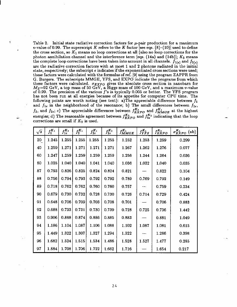
; Table 2. Initial state radiative correction factors for /.L- P

air production for a maximum . v-value of 0.99. The superscript K refers to the K factor see eqs. (8)-(lo)] used to define

the cross section, so K1 means no loop corrections at all ( a so no loop corrections for the 1 photon annihilation channel and the interference term [eqs. (14a) and (14b)j; KS means the complete loop corrections have been taken into account in all channels. flte. and f2te) are the radiative correction factors with at most 1 and 2 photons radiated in the initial state, respectively; the subscript e indicates if the exponentiated cross sections were used; these factors were calculated with the formulas of ref. [9] using the program ZAPPR from G. Burgers. The subscripts MMGE, YFS, and EXPO indicate the programs from which these factors were calculated. (rEXp0 gives the absolute cross section in nanobarn for Mz=92 GeV, a top mass of 50 GeV, a Higgs mass of 100 GeV, and a maximum v-value of 0.99. The precision of the various f’s is typically 0.005 or better. The YFS program has not been run at all energies because of its appetite for computer CPU time. The following points are worth noting (see text): a)The appreciable difference between fi and fre in the neighborhood of the resonance; b) The small differences between fie, f2, and fse; c) The appreciable differences between fiipo and fzM,, at the highest

- energies; d) The reasonable agreement between fE-$po and f2T indicating that the loop corrections are small if K2 is used.

-

fi fF1 f:l fF1 fE1 fz fzMGE f;+S f$&‘O a&‘O bb) 20 1.245 1.255 1.255 1.255 1.255 1.252 1.253 1.259 0.299 - 40 1.259 1.271 1.271 1.271 1.271 1.267 1.262 1.276 0.077

60 1.247 1.259 1.259 1.259 1..259 1.256 1.244 1.264 0.036

80 1.025 1.040 1.040 1.041 1.040 1.036 1.032 1.040 0.035

87 0.793 0.826 0.825 0.824 0.824 0.821 - 0.822 0.104

88 0.756 0.794 0.793 0.792 0.792 0.789 0.769 0.792 0.149

89 0.718 0.762 0.762 0.760 0.760 0.757 - 0.759 0.234

90 0.679 0.730 0.732 0.728 0.730 0.726 0.714 0.729 0.424

91 0.648 0.706 0.709 0.703 0.708 0.701 - 0.706 0.883

92 0.688 0.733 0.731 0.730 0.739 0.728 0.725 0.736 1.442

93 0.906 0.888 0.874 0.886 0.885 0.883 - 0.881 1.049

94 1.186 1.104 1.087 1.106 1.088 1.102 1.087 1.081 Q.615

95 1.449 1.322 1.307 1.327 1.294 1.322 - 1.286 0.398

96 1.682 1.524 1.515 1.534 1.486 1.528 1.527 1.477 0.285

97 1.884 1.708 1.706 1.722 1.662 1.716 - 1.654 0.217

24

Table 3. MC GENERATORS: e+e-- -+ 72’ --+ p+p- .

Program Authors Ref. Initial State Final State Loop Corr. Pol. Radiation Radiation

MMG F. A. Berends R. Kleiss 10 ok4 + - - S. Jadach

MMGE

BREM5

J. Alexander 11 O(a2) + exp. - - -

R. Kleiss B. W. Lynn 8 O(Q) + + + R. G. Stuart

EXPOSTAR C. J. C. Im 8 structure - D. Kennedy

+ + functions

BREMGt BREM5 structure EXPOSTAR - functions

+ + +

YFS* S. Jadach 12 multiple - - B. F. L. Ward photons

+

BHKMUONt F. A. Berends W. Hollik - R. Kleiss

ok4 + + -

t not yet released. * A new version, together with Z. Was, will include the loop corrections.

25

FIGURE CAPTI.ONS

1. The expected number of events as function of center of mass energy for Mz = 92 GeV

and a luminosity of 1.1 nb-l for each energy point. The vertical error barr indicates

the statistical error, while the horizontal error bar indicates the expected error on

Mz, if one calculates MZ from that single energy point assuming the width to be

. known.

-

2. A summary of the present knowledge about MZ from the pj?~ collider experiments UAl

and UA2, the combined neutral current data2 ( sin2 ew), and the rise in the hadronic

cross section at PETRA and KEK (R) (calculated from the results described in _

ref. [4]).

3. The u-distribution in first and second order. In first order, v is the photon energy

- normalized to the beam energy. The solid curves were calculated from the formulae

in ref. 191. The dots were obtained from the MMGE Monte Carlo generator.

4. As in Fig. 3 but for the exponentiatied cross sections normalized to the first order

cross section.

5. The v-distribution of the MMGE Monte Carlo generators MMGE (a) and YFS (b)

normalized to the exact second order calculation of ref. [9]. One sees good agreement

with the expected straight line. In fig. 5b we have also plotted the result, if the

energy of the photons radiated in addition to the first photon is limited to 3 GeV.

From the difference one sees that the contribution from two or more hard photons

is appreciable. These comparisons were done at ,,/Z = 60 GeV; at this energy the

contribution from hard photon radiation is large in contrast to the radiation from

the Z” resonance, where the radiation of hard photons is negligible because of the

_- sharpe decrease in the cross section at lower energies.

6. The fitted values of MZ and Tz and their correlation p as function of E for three scan

points separated by A = 1.5 GeV. c is the distance of the central point to the peak, so

the location of the scan points on the resonance is as indicated on the left in (a) for

E = 1, 0, and -1 GeV. Each error bar is the result of a fit to Monte Carlo generated

26

events with a total luminosity of 3.3 nb-l equally divided over three energy scan

points. This luminosity corresponds to 100 events at the peak, but only w 80 and

60 events, if the luminosity is divided over three scan points with c = 0, and 1 GeV,

respectively.

7. As in fig. 6, but for a smaller scan range: A = 1 GeV. In this case the correlation

between MZ and I’z becomes appreciably larger.

8. The expected error on MZ and rz and their correlation p as a function of the scan

range, which is defined as the difference in energy between the highest and lowest

point. The lower curve shows the decrease in event numbers with increasing scan

range. The three scan points were taken symmetrically around the peak (E = 0 GeV).

9. As fig. 8, but for E = 0.5 GeV.

10, As fig. 8, but for E = 1.0 GeV.

11. The expected error on the width for different event samples (expressed in number of

“peak” events Nt) and different normalization errors (a,), which cause a correlation

between the different energy points. The crosses indicate the error from the shape

fit alone, thus disregarding the information from the absolute value of the cross

section. Note that the fit using the normalization is always better than the shape

fit, even in case of large normalization errors and high statistics (see text).

27

i

.

40

30

N

20 -

IO

0

-

88 6-88

1 1

I I I I I 1 I I I

90 92 94 6 (GeV)

96 98 6029Al

Fig. 1

.

I I I I I I I I I

-

UA2 a w -

sin28w a w

I I I I I 1 I I I

88 90 92 94 96

6-88 Mz 6029A2

Fig. 2

-

10-l

7-88

l MMGE

0 0.2 0.4 0.6 0.8 1.0 v 6029A3

Fig. 3

,.

I .4

1.2 2nd Order Exponentiated

6- $ 1.0

,. 0.8

. 0.6

0 0.2 0.4 0.6 0.8 1.0 - 7-88 v 6029A4

-

Fig. 4

2.0 .

1.5

%z 2 g 1.0

_ 5 b

0.5

0

9-88

I I I I I I I I I

(0)

A T

-

I I I I I I I I

0 0.2 0.4 0.6 0.8 1.0 v 6029A2 1 ‘-

Fig. 5

.

-

N+ = 100, A = 1.5 GeV I I I I I I I I I

-I

I I I I I I I

90 91 92 93 94

-

I

1 20

w

-I

- I I I I I I I I I

2 3 I’, (GeV)

I I I I I

,W. 8’ (Cl

) =r&

l .@@;+$.*

l a< , 0. ’ 0 2 .+ 0. 8

I I I I I

-

-1.0 -0.5 0 0.5 1.0 5-66 P 6029613

Fig. 6

I

- v

-I

N, = 100, A= 1 GeV I

(0)

-A I I I

90 91 92 93 94

1

2 20-

v F I -’ t-

I I I I I I I I I

-1.0 -0.5 0 0.5 1.0 5-m P 6029812

Fig. 7

c =(A)-M,o= OGeV

.

- 0.4 L

a 0.2

0.4

Q 0

-0.4

0.8

5-88

O Nt = 100 c”=l5%

x Nt = 400 on = 5% A N,= 1000 a;l = 3%

A Y

I I I I I

X n A I\ A X

I I I I

0 2 4 6 SCAN RANGE (GeV)

Fig. 8

6029A8

.

-

0.8

c = (A) - M,o = 0.5 GeV o Nt= too 0” = 15% x N,= 400 a, = 5% A N,=lOOO on = 3%

J I I I I I I 0 2 4 6

5-88 SCAN RANGE (GeV) 6029A9

-

Fig. 9

.

0.4

0.4 -

L a 0.2

c =(,A>-M,o- 1 GeV

O Nt = IO0 cn= 15% x N,= 400 a” = 5% A N,=lOOO q, = 3%

I I I I I I I

I Q I I I

11:

I I I I I I I

0.8

“0 2 4 6 5-88 SCAN RANGE (GeV) 6029AlO

Fig. 10

I

A q, = 3 ‘10 q a;, =25% 0 cr”=l5% x Shape Fit

.

-

0.08

0.04

0

0.2

0.1

‘d O 0.4

0.2

0

0.8

0.4

0 -

\ Nt = I@ Z” 1

N, = IO4 Z” --I _-- ---------------

t + bu I \\ -I

Nt =103 Z” -I

r * vu 4 - --- -I

A A A A A A I I I I I

Y, -7 -n

r vu .--

Nt = IO’ Z’ ,

.&iziizP m-b --- --m-----

0 2 4 6 5-88 SCAN RANGE (GeV) 6029All

Fig. 11