Embed Size (px)
Citation preview
Graduate Theses, Dissertations, and Problem Reports
2016
Determination of Material Parameters of E-GlassEpoxy Laminated Determination of Material Parameters of E-GlassEpoxy Laminated
Composites in ANSYS Composites in ANSYS
Mehdi Shahbazi
Follow this and additional works at: https://researchrepository.wvu.edu/etd
Recommended Citation Recommended Citation Shahbazi, Mehdi, "Determination of Material Parameters of E-GlassEpoxy Laminated Composites in ANSYS" (2016). Graduate Theses, Dissertations, and Problem Reports. 6610. https://researchrepository.wvu.edu/etd/6610
This Thesis is protected by copyright and/or related rights. It has been brought to you by the The Research Repository @ WVU with permission from the rights-holder(s). You are free to use this Thesis in any way that is permitted by the copyright and related rights legislation that applies to your use. For other uses you must obtain permission from the rights-holder(s) directly, unless additional rights are indicated by a Creative Commons license in the record and/ or on the work itself. This Thesis has been accepted for inclusion in WVU Graduate Theses, Dissertations, and Problem Reports collection by an authorized administrator of The Research Repository @ WVU. For more information, please contact [email protected].
Determination of Material Parameters of E-Glass/Epoxy
Laminated Composites in ANSYS
Mehdi Shahbazi
Thesis submitted
to the College of Engineering and Mineral Resources at West Virginia University
in Partial Fulfillmen t of requirements for the degree of
Master of Science in
Mechanical Engineering
Ever J. Barbero, Ph.D., Chair
Konstantinos Sierros, Ph.D.
Marvin Cheng, Ph.D.
Department of Mechanical and Aerospace Engineering (MAE)
Morgantown, West Virginia , 2016
Keywords: ANSYS, Composite, Progressive Damage Analysis, Discrete Damage
Mechanics, Damage Behavior, E Glass Epoxy
Copyright 2016 Mehdi Shahbazi
c
Abstract
Determination of Material Parameters of E Glass/Epoxy Laminated
Composites in ANSYS
Mehdi Shahbazi
Prediction of damage initiation and Evolution in composite materials are of particu-
lar importance for the design, production, certification, and monitoring of an increasingly
large variety of structures. In this study a methodology is presented to calculate the mate-
rial properties for the progressive damage analysis (PDA) and discrete damage mechanics
(DDM) in ANSYSQR by using two sets of experimental data for laminates [02/904]S and
[0/ ± 404/01/2]S . The type of laminates to be used for material property determination are
chosen based on a sensitivity study.
This method is based on fi results calculated with PDA and DDM to experimental
data by using Design of Experiments and optimization tools in ANSYS Workbench. The
method uses experimental modulus-reduction vs. strain data for only two laminates to
fi all the parameters of PDA (F2t, F6, Gtm) and DDM (GIc, GIIc) . Fitted parameters
are then used to predict and compare with the experimental behavior of other laminates
with the same material system. Mesh sensitivity of both PDA and DDM is studied by
performing p- and h-mesh refinement. Choice of damage activation function is justified
based on goodness of fi with each proposed equation. Comparison between DDM and
PDA predictions is shown.

iii
Acknowledgements
I would like to thank all the people who made this possible.

iv
Dedication
This is dedicated to my parents Khodadad Shahbazi and Ghadam-kheir khorshidi.
v
Table of Contents List of Tables vii
List of Figures ix
1 Introduction 1
2 Progressive Damage Analysis (PDA) 3
2.1 Progressive Damage Analysis in ANSYS . . . . . . . . . . . . . . . . . . . 4
2.1.1 Damage Initiation Criteria . . . . . . . . . . . . . . . . . . . . . . . 4
2.1.2 Material Strength Limits . . . . . . . . . . . . . . . . . . . . . . . . 6
2.1.3 Damage Evolution . . . . . . . . . . . . . . . . . . . . . . . . . . . 7
2.2 PDA Design of Experiments..................................................................................10
2.3 Methodology ............................................................................................................... 13
2.3.1 APDL .............................................................................................................. 14
2.3.2 Workbench ........................................................................................................... 15
2.3.3 Optimization ...............................................................................................16
2.4 Comparison with experiments ...............................................................................23
2.5 Mesh sensitivity .......................................................................................................... 26
3 Discrete Damage Mechanics (DDM) 29
3.1 Discrete Damage Mechanics .......................................................................................30
vi
3.1.1 Description of DDM Model ...........................................................................30
3.2 DDM Design of Experiments ......................................................................................34
3.3 Methodology ................................................................................................................37
3.3.1 APDL ...............................................................................................................38
3.3.2 Workbench ........................................................................................................... 40
3.3.3 Optimization ............................................................................................... 41
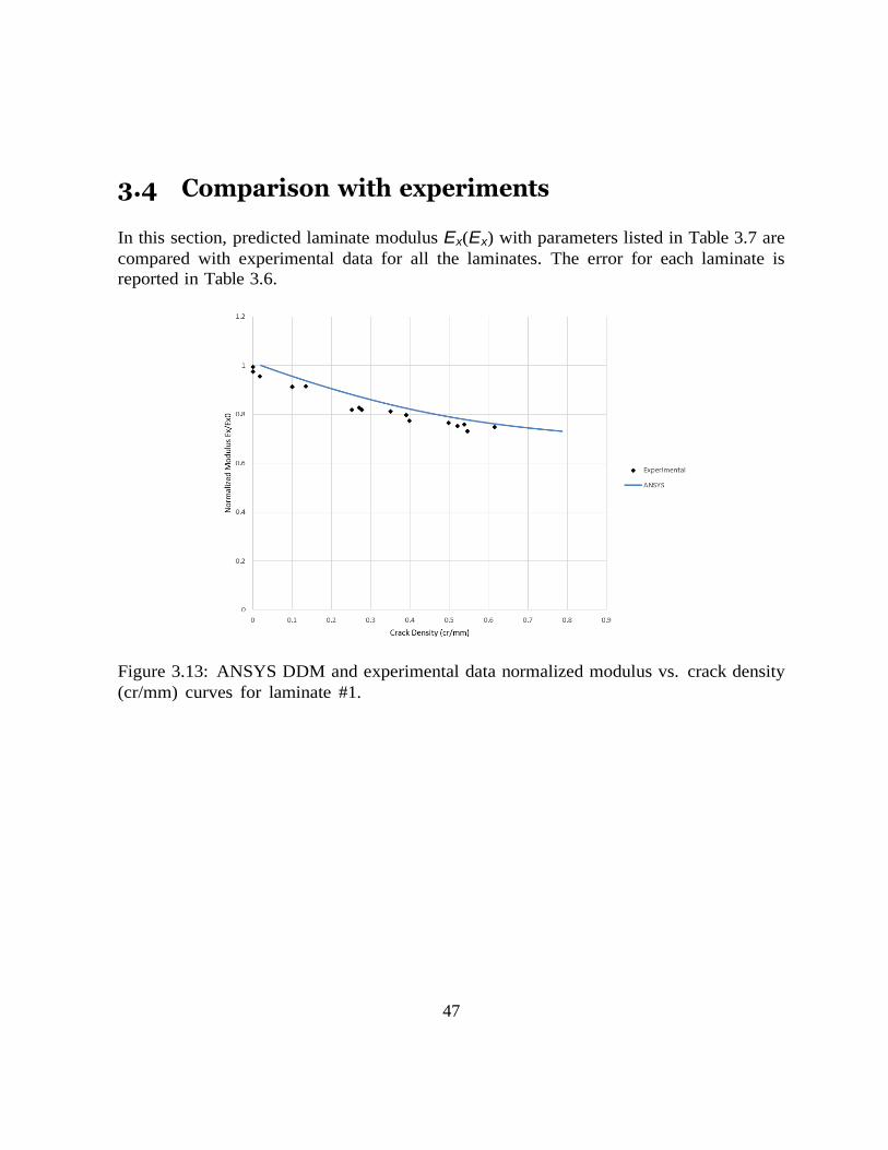
3.4 Comparison with experiments ............................................................................... 47
3.5 Mesh sensitivity ...........................................................................................................57
3.6 Effect of damage activation function ..................................................................... 59
4 Conclusions and Future Work 61
4.1 Conclusions ..................................................................................................................61
4.2 Comparison between DDM and PDA ......................................................................... 62
4.3 Future Work .......................................................................................................................... 70
APPENDICES 72
A 73
A.1 Progressive Damage Analysis (PDA) APDL Code .............................................. 73
A.2 Discrete Damage Mechanics (DDM) Model APDL Code ........................................78
B 83
B.1 Optimization ........................................................................................................... 83
References 87
vii
List of Tables
2.1 Number of FEA evaluations used (a) to construct the response surface (RS)
and (b) to adjust the input parameters by direct optimization (DO). ................ 11
2.2 Laminate stacking sequence for all laminates for which experimental data is
available. ........................................................................................................................... 13
2.3 Sensitivity S of the output (error) to each input (parameter). First two rows
refer to laminate #1 and last row to laminate #8. ............................................. 13
2.4 Lamina elastic properties and in-situ strength values. ........................................... 15
2.5 Damage evolution properties of the lamina. ............................................................ 15
2.6 Error and adjusted values of input (material) parameters for all laminates
considered. ................................................................................................................... 18
2.7 Comparison of adjusted input (material) parameters obtained by using Re-
sponse Surface Optimization (RSO) and Direct Optimization (DO). .................. 18
3.1 Number of FEA evaluations used (a) to construct the response surface (RS)
and (b) to adjust the input parameters by direct optimization (DO). Inter-
acting equation (3.2) is used. ................................................................................. 35
3.2 Laminate stacking sequence for all laminates for which experimental data is
available. ........................................................................................................................... 37
3.3 Sensitivity S of the output (error) to each input (parameter). First row
refers to laminate #1 and last row to laminate #8. Interacting equation
(3.2) is used. ........................................................................................................ 37
3.4 Lamina elastic properties and in-situ strength values. ........................................... 39
3.5 Damage evolution properties of the lamina. ............................................................ 40
viii
3.6 Error and adjusted values of input (material) parameters for all laminates
considered. Eq. (3.2) is used. Values of GIc and GIIc are given in Table 3.7. 42
3.7 Comparison of adjusted input (material) parameters obtained by using Re-
sponse Surface Optimization (RSO) and Direct Optimization (DO). Eq.
(3.2) is used. ........................................................................................................... 43
ix
c
c
m
List of Figures
2.1 Equivalent stress σe vs. equivalent displacement ue. . . . . . . . . . . . . . 8
2.2 Response surface chart. Error (D) vs. F2t ............................................................. 11
2.3 Response surface chart. Error (D) vs. Gmt ........................................................... 12
2.4 Response surface chart. Error (D) vs. F6 ................................................................ 12
2.5 Normalized modulus vs. applied strain for laminate #1. ..................................... 14
2.6 Importing the APDL code into Workbench. ............................................................ 16
2.7 Inputs and output parameters are selected. .......................................................... 16
2.8 Response Surface tools include DoE, RS, and RS Optimization. ......................... 17
2.9 Sensitivity of output (error D) to inputs F2t, Gtm, and F6 .................................. 19
2.10 Candidate design points. ........................................................................................ 19
2.11 Sensitivity curves show how sensitive the output D is to inputs F2t, Gt , and
F6 for laminate #8. ................................................................................................ 20
2.12 Setting the limits (range) for the input parameters. ............................................. 21
2.13 Selecting the optimization method. ....................................................................... 22
2.14 Error (D) is selected to be minimized. .................................................................. 22
2.15 Normalized modulus vs. applied strain for laminate #2. ..................................... 23
2.16 Normalized modulus vs. applied strain for laminate #3. ..................................... 24
2.17 Normalized modulus vs. applied strain for laminate #4. ..................................... 24
2.18 Normalized modulus vs. applied strain for laminate #8. ..................................... 25
2.19 Normalized modulus vs. applied strain for laminate #9. ..................................... 25
x
2.20 Force vs. applied strain for laminate #1 using diff t number of elements. 27
2.21 Normalized Modulus vs. applied strain for laminate #1 using diff t num-
ber of elements.............................................................................................................28
3.1 Representative volume element (RVE) between two adjacent cracks. ................. 31
3.2 Response surface chart. Error (D) vs. GIC ...................................................... 36
3.3 Response surface chart. Error (D) vs. GIIC ................................................ 36
3.4 Normalized modulus vs. applied strain for laminate #1 (interacting eq.3.2]). 39
3.5 Importing the APDL code into Workbench. ........................................................... 40
3.6 Inputs and output parameters are selected. ........................................................... 41
3.7 Response Surface tools include DoE, RS, and RS Optimization. ........................ 41
3.8 Sensitivity of output (error D) to inputs GIC and GIIC .................................... 43
3.9 Candidate design points. ........................................................................................ 44
3.10 Setting the limits (range) for the input parameters. .............................................. 45
3.11 Selecting the optimization method. ....................................................................... 46
3.12 Error (D) is selected to be minimized. .................................................................. 46
3.13 ANSYS DDM and experimental data normalized modulus vs. crack density
(cr/mm) curves for laminate #1. ............................................................................ 47
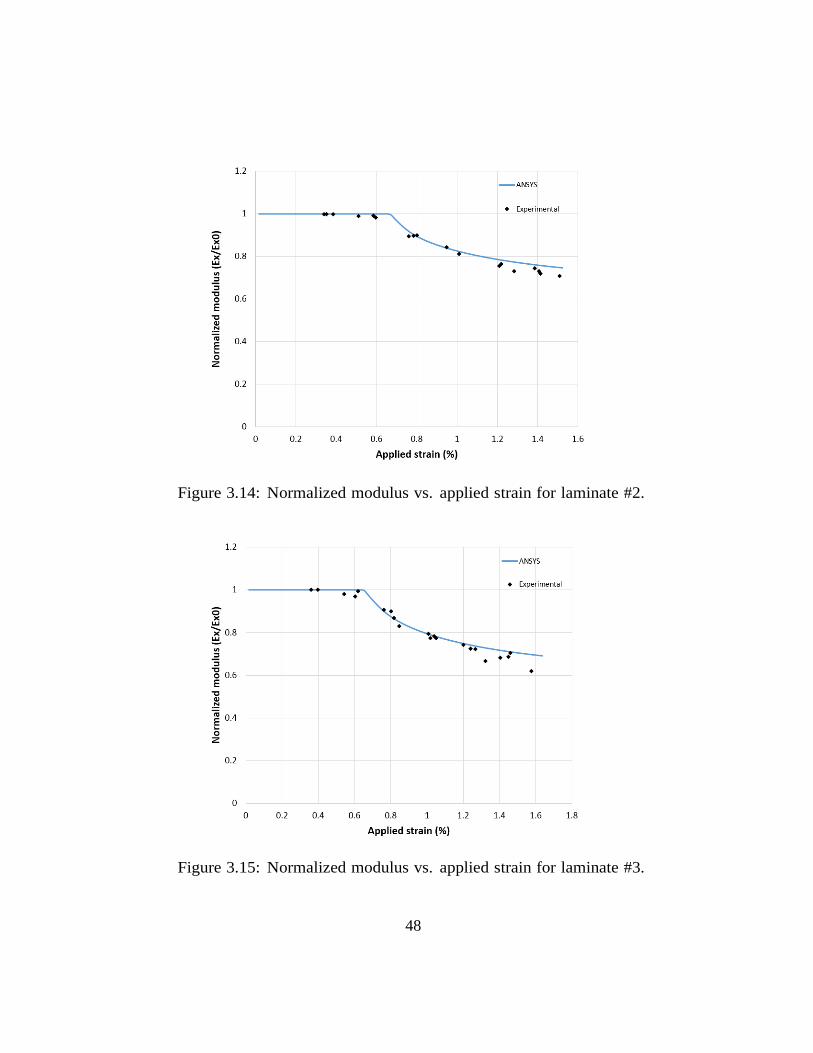
3.14 Normalized modulus vs. applied strain for laminate #2. ..................................... 48
3.15 Normalized modulus vs. applied strain for laminate #3. ..................................... 48
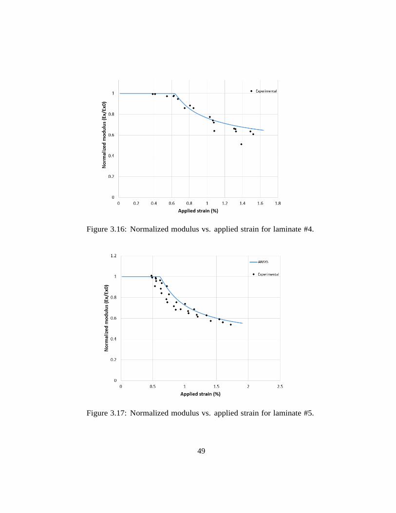
3.16 Normalized modulus vs. applied strain for laminate #4. ..................................... 49
3.17 Normalized modulus vs. applied strain for laminate #5. ..................................... 49
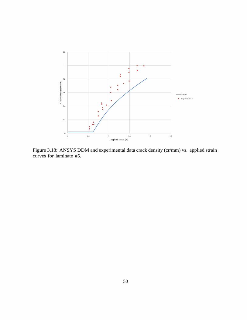
3.18 ANSYS DDM and experimental data crack density (cr/mm) vs. applied
strain curves for laminate #5. ................................................................................ 50
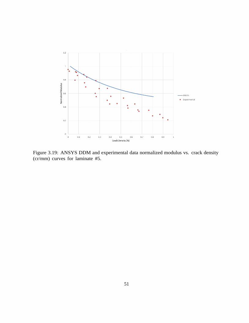
3.19 ANSYS DDM and experimental data normalized modulus vs. crack density
(cr/mm) curves for laminate #5. ............................................................................ 51
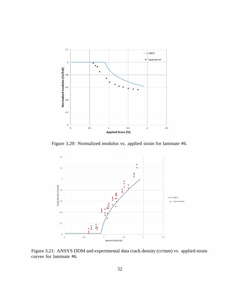
3.20 Normalized modulus vs. applied strain for laminate #6. ..................................... 52
3.21 ANSYS DDM and experimental data crack density (cr/mm) vs. applied
strain curves for laminate #6. ................................................................................ 52
3.22 ANSYS DDM and experimental data normalized modulus vs. crack density
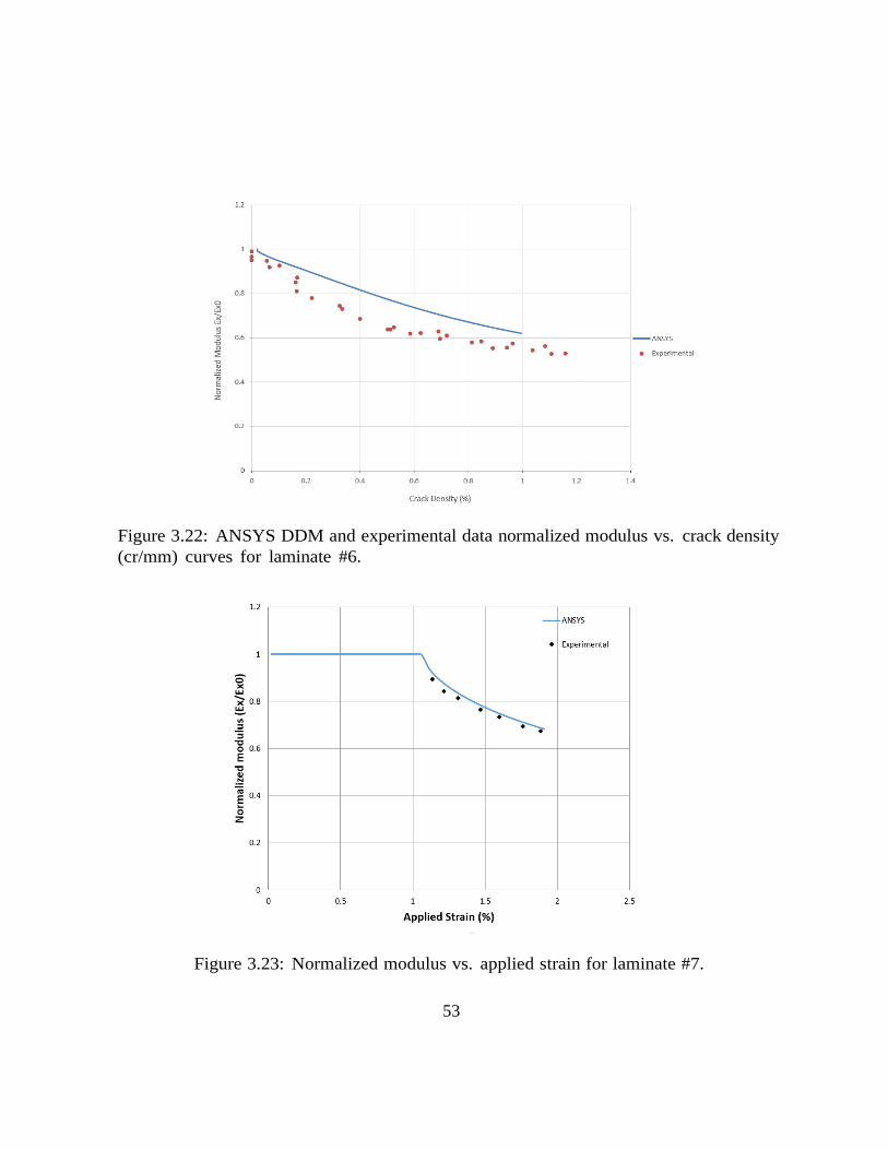
(cr/mm) curves for laminate #6. ............................................................................ 53
3.23 Normalized modulus vs. applied strain for laminate #7. ..................................... 53
3.24 ANSYS DDM and experimental data crack density (cr/mm) vs. applied
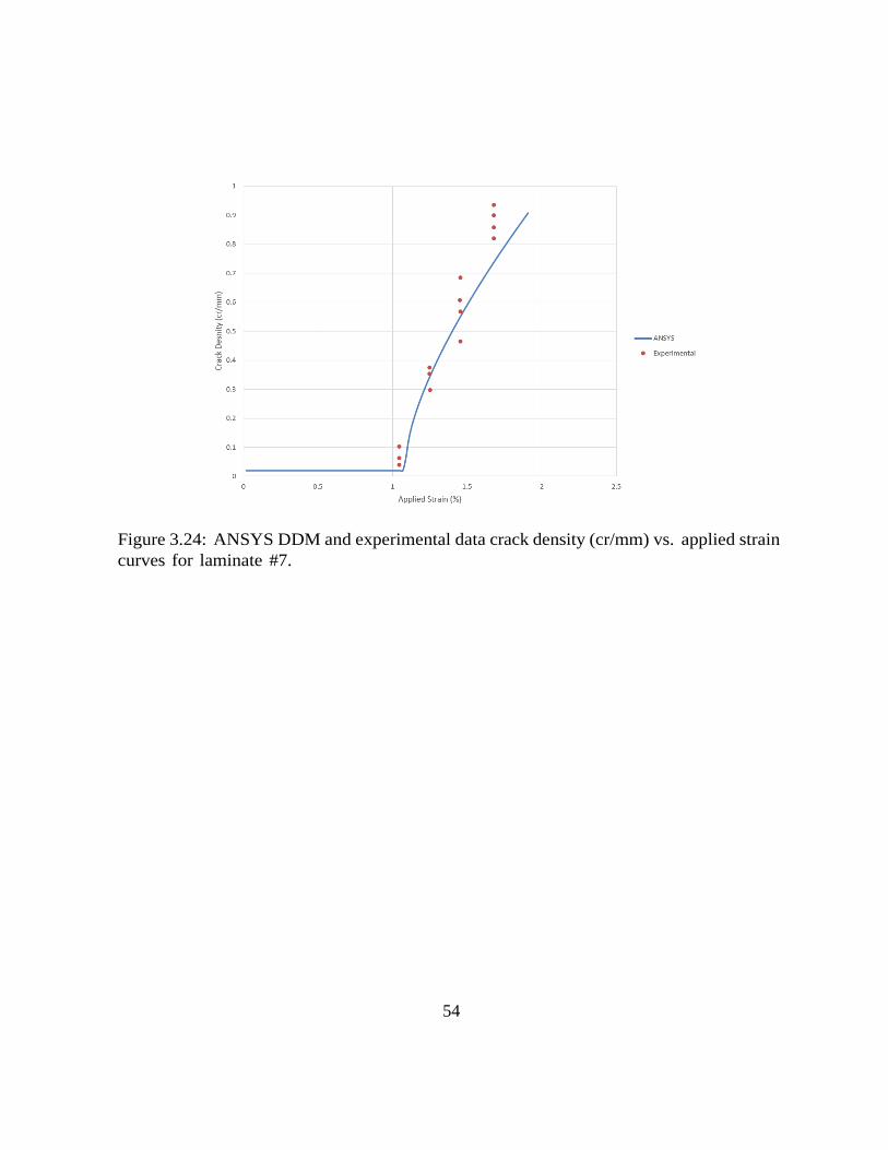
strain curves for laminate #7. ................................................................................ 54
3.25 ANSYS DDM and experimental data normalized modulus vs. crack density
(cr/mm) curves for laminate #7. ............................................................................ 55
3.26 Experimental data of Normalized modulus vs. Crack density for laminate #7. 55
3.27 Normalized modulus vs. applied strain for laminate #8. ..................................... 56
3.28 Normalized modulus vs. applied strain for laminate #9. ..................................... 56
3.29 Force Fx vs. applied strain for laminate #1 using diff t number of elements 58
3.30 Normalized Modulus vs. applied strain for laminate #1 using diff t num-
ber of elements for PLANE 182 and one element for PLANE 183. ........................59
3.31 Normalized Modulus vs. applied strain for laminate #7 3.1, 3.2, and PDA
results. ..................................................................................................................... 60
4.1 ANSYS DDM and PDA, Normalized modulus vs.
#1. . . . . . . . . . . . . . . . . . . . . . . . . .
applied strain for laminate
. . . . . . . . . . . . . . .
62
4.2 ANSYS DDM and PDA, Normalized modulus vs.
#2. . . . . . . . . . . . . . . . . . . . . . . . . .
applied strain for laminate
. . . . . . . . . . . . . . .
63
4.3 ANSYS DDM and PDA, Normalized modulus vs.
#3. . . . . . . . . . . . . . . . . . . . . . . . . .
applied strain for laminate
. . . . . . . . . . . . . . .
64
4.4 ANSYS DDM and PDA, Normalized modulus vs.
#4. . . . . . . . . . . . . . . . . . . . . . . . . .
applied strain for laminate
. . . . . . . . . . . . . . .
65
4.5 ANSYS DDM and PDA, Normalized modulus vs.
#5. . . . . . . . . . . . . . . . . . . . . . . . . .
applied strain for laminate
. . . . . . . . . . . . . . .
66
4.6 ANSYS DDM and PDA, Normalized modulus vs.
#6. . . . . . . . . . . . . . . . . . . . . . . . . .
applied strain for laminate
. . . . . . . . . . . . . . .
67
4.7 ANSYS DDM and PDA, Normalized modulus vs.
#7. . . . . . . . . . . . . . . . . . . . . . . . . .
applied strain for laminate
. . . . . . . . . . . . . . .
68
4.8 ANSYS DDM and PDA, Normalized modulus vs.
#8. . . . . . . . . . . . . . . . . . . . . . . . . .
applied strain for laminate
. . . . . . . . . . . . . . .
69
xi
4.9 ANSYS DDM and PDA, Normalized modulus vs. applied strain for laminate
#9. . . . . . . . . . . . . . . . . . . . . . . . . . . . . . . . . . . . . . . . . 70
B.1 Importing the apdl code to Workbench ................................................................... 83
B.2 Inputs and output(error) are selected for optimization purpose ........................... 84
B.3 Design Exploration tools ....................................................................................... 84
B.4 In Design of Experiment part the user can set the limits for inputs .................... 85
B.5 Updating all the previous steps and selecting the optimization ........................... 86
B.6 Error (D) is selected to be minimized ................................................................... 86
xii
1
Chapter 1
Introduction
A composite material is a combination of two or more materials, whose properties are su-
perior to those of the constituent materials acting independently. Fibre-reinforced polymer
composites are usually manufactured by strong fi and less stiff polymeric matrix. The
primary role of the fi is to provide strength and stiffness to the composite. Typical
reinforcing fi used are glass, carbon and aramid. The most common types of glass fi er
used in fi erglass which is considered in this study is E-glass, which is alumino-borosilicate
glass with less than 1% w/w alkali oxides, mainly used for glass-reinforced plastics.
Damage initiation and propagation are two important concerns in predicting damage
behavior of composite materials, so prediction of damage initiation and propagation are of
particular importance for the design, production certification and monitoring of an increas-
ingly large variety of structures. This study focuses on adjusting the material parameters
for the discrete damage mechanics (DDM) and progressive damage analysis (PDA) models
to precisely predict the damage behavior .
ANSYS Mechanical provides progressive damage analysis (PDA, [2]) starting with re-
lease 15. Also, the user can defi DDM model as a user material in ANSYS and use
that in an APDL code. In this study a DDM model is defi as a dll fi and is used to
analyze the damage. Furthermore, ANSYS Workbench allows optimization of any set of
variables to any user defi objective defi in a Mechanical APDL (MAPDL) model
by importing the APDL script into Workbench and using Design of Experiments (DoE)
and Direct Optimization (DO). Since PDA is not implemented in the graphical user inter-
face (GUI), the user must use APDL commands to defi the damage initiation criterion,
damage evolution law, and material properties.
Although elastic moduli are available for many composite material systems, the same
2
c
c
is not true for the material properties required by PDA and DDM models. However,
laminate modulus and Poisson’s ratio degradation of laminated composites as a function
of applied strain are available for several material systems [24, 25]. This study shows how
to use available data to infer the material properties required by PDA. Specifically, the
main purpose of this study is to fi in-situ values [7] of transverse tensile strength F2t, in-
plane shear strength F6, and energy dissipation per unit area Gtm for the material system
(composite lamina) that can be used in PDA to predict damage initiation and evolution
of laminated composite structures built with the same material system.
The stated objective for PDA is achieved by minimizing the error between PDA pre-
dictions and available experimental data. Once the input parameters F2t, F6 and Gtm are
found, the accuracy of PDA predictions is checked by comparing those predictions with
experimental data for other laminates that has not been used to fi the input parameters.
Also, by minimizing the error between DDM model predictions and available experimental
data the input parameters GIc and GIIc are found for DDM model, and the accuracy of
DDM predictions is checked by the same method mentioned for PDA model.
In fact, experimental data for only two laminates are required to fi the parameters.
Although the input parameters are fi using an specific mesh (one element) and type
of element (SHELL 181 for PDA and PLANE 182 for DDM), it is expected that the PDA
and DDM constitutive model will be mesh insensitive in order to be useful when mesh
refinement and several type of elements are used for the analysis of a complex structure.
Mesh sensitivity is thus assessed in this work by performing both p- and h-refi t.
3
Chapter 2 Progressive Damage Analysis (PDA)
There are lots of failure theories([15], [14], [8], [16]) which are used not only for predicting
the initiation of damage but also for progressive failure up to ultimate load. The most
popular failure criteria are the those criteria which are easier to use, although it does not
mean that they are accurate. The theories such as the maximum stress, the maximum
strain, TsaiWu, TsaiHill, and the Hashin failure criteria are still widely used despite their
limits because they are simple, easy to understand and implement in analysis ([8],[16]).
The maximum stress and maximum strain criteria are typical examples of so-called non-
interactive theories which have been shown to produce poor predictions in general [13],
these two criteria only predict the damage initiation.
Theories that allow interaction between stress components such as the TsaiWu criterion
generally perform better results ([23], [22]). In a review [8], wide variations in prediction
by various theories are attributed to diff t methods of modeling the progressive damage
process, the nonlinear behavior of matrix-dominated laminates (angle plys), the inclusion or
exclusion of curing residual stresses in the analysis, and the defi of ultimate laminate
failure (ULF). The latter may be defi in at least three diff t ways: the maximum load
attained; the occurrence (or detection) of fi fi er failure (FFF); and the occurrence of last
ply failure (LPF). The review also discusses the effects of interactions, with good reported
agreement with experiment in the shear-tension quadrant, but less agreement in the shear-
compression quadrant. Similar conclusions are reached in another review of failure theories
by Icardi et al. ([8], [16]). Recently, the phrase physically based (and mechanism based or
similar words) has been used to describe failure theories which have separate predictions
of fi er-dominated and matrix-dominated failures ([16], [19], [18] and [17]). Hashins [11]
and Pucks [20] criteria are in this category and accounts for their popularity in progressive
4
F t =
damage modeling. This study focuses on Hashin [12], since ANSYS uses Hashin criterion
for progressive damage analysis (PDA).
2.1 Progressive Damage Analysis in ANSYS To perform progressive damage analysis of composite materials, the user needs to provide
linear elastic orthotropic material properties and three material models: damage initiation,
damage evolution law, and material strength limits.
2.1.1 Damage Initiation Criteria With damage initiation criteria the user can defi how PDA determines the onset (initia-
tion) of material damage. The available initiation criteria in ANSYS are maximum strain,
maximum stress, Hashin, Puck, LaRC03, and LaRC04. Besides, the user can defi up
to nine additional criteria as user defi initiation criteria, but only the Hashin crite-
rion works with PDA. The remaining only work with instant stiffness reduction (MPDG).
The later is similar to ply-drop off but the amount of stiffness drop can be specified in
the range 0–100% of the undamaged stiffness. With MPDG, the user can choose failure
criteria among those mentioned for each of the damage modes, which are assumed to be
uncoupled.
For example, using the Hashin initiation criteria, we have the following four modes of
failure: fi er tension, fi er compression, matrix tension, and matrix compression, which
are represented by damage initiation indexes Fft, Ffc, Fmt and Fmc that indicate whether a
damage initiation criterion in a damage mode has been satisfied or not. Damage initiation
occurs when any of the indexes exceeds 1.0. Damage initiation indexes are unfortunately
called “failure” indexes in the literature, despite the fact that nothing “fails” but rather a
small amount of damage appears.
Fiber tension (σ11 ≥ 0)
Fiber tension is a misnomer sometimes used in the literature, since this mode actually
represents longitudinal tension of the composite lamina, not the fi er. The corresponding
damage initiation index is computes as follows
σ11
2
f F1t
σ12
2 + α
F6
(2.1)
5
F c
F t
F c
=
=
= 1
Fiber Compression (σ11 < 0) Fiber compression is a misnomer, since this mode actually represents longitudinal compres-
sion of the composite lamina, not the fi er. The corresponding damage initiation index is
computes as follows
σ11 2
f F1c
(2.2)
Matrix tension and/or shear (σ22 ≥ 0)
This is also misnomer, since this mode actually represents transverse tension and in-plane
shear of the composite lamina, not the matrix. the confusion is doe to the fact that this
is a matrix-dominated mode but still the criteria applied at the meso-scale, that is at the
level of a lamina, not at the micro-scale where the fi er and matrix would be analyzed
separately. Furthermore, the properties involved (F2t, F6) are those of a lamina, not of
fi er and matrix separately, ans also the resulting index applies to the lamina, not to the
matrix.
σ22 2
m F2t
σ12
2 +
F6
(2.3)
Matrix compression (σ22 < 0) Matrix compression is a misnomer, since this mode actually represents transverse compres-
sion and transverse shear of the composite lamina, not the matrix.
σ22
2
m 2F4
I F2c
2 +
2F4
σ22
— F2c
σ12
2 +
F6
(2.4)
where σij are the components of the stress tensor; F1t and F1c are the tensile and com-
pressive strengths of a lamina in the fi er direction; F2t and F2c are the in-situ tensile and
compressive strengths in the matrix direction; F6 and F4 are the in-situ longitudinal and
transverse shear strengths, and α determines the contribution of the shear stress to the fi er

6
tensile criterion. To obtain the model proposed by Hashin and Rotem [12] we set α = 0
6
and F4 = 1/2F2c. Note that in-situ properties should be used for all matrix-dominated
modes.
This study uses Hashin initiation criteria for all tensile and compression failures. The
command APDL for this purpose is TB, DMGI, as it is shown below:
! Damage detection using failure criteria
TB, DMGI, 1, 1, 4, FCRT
TBTEMP,0
! 4 is the value for selecting Hashin criteria,
! which is here selected for all four failure modes
TBDATA,1,4,4,4,4
2.1.2 Material Strength Limits To evaluate the damage initiation criteria, the user defi the maximum stresses or strains
that a material can tolerate before damage occurs. Required inputs depend on the chosen
criteria in the damage initiation part. For instance, for Hashin criteria the user needs to
defi in-situ tensile and compression strength in 1, 2, and 3 lamina orientations (called
X, Y, and Z directions in ANSYS), and the shear strength in 12, 13, and 23 lamina planes
(called XY, XZ, and YZ in ANSYS).
Since fi er dominated properties are at least one order of magnitude (10X) larger than
matrix dominated properties, matrix modes occur much earlier in the life of the structure
that fi er modes. Fiber modes (§2.1.1, §2.1.1) do not occur until nearly the end of the life.
Furthermore, transverse matrix compression (§2.1.1) does not result in progressive damage
but rather leads to sudden failure according to the Mohr-Coulomb criterion [9]. Therefore,
this study focuses on matrix tension and shear modes (§2.1.1), which are know to lead to
substantial progressive damage [24, 25].
Initial values of in-situ transverse tensile strength F2t, in-situ in-plane shear strength F6,
and intralaminar shear strength F4 (called XT, XY, and XZ in ANSYS) should be defi
in the APDL script. The command for material strength limit is TB, FCLI, as shown below:
! Material Strengths TB,FCLI,1,1,6 TBTEMP,0 ! Failure Stress, Fiber Tension TBDATA,1, F1t
7
! Failure Stress, Fiber Compression TBDATA,2,F1c
! Toughness Stress, Matrix Tension TBDATA,3,F2t
! Failure Stress, Matrix Compression TBDATA,4,F2c
! Failure Stress, XY Shear TBDATA,7,F6
! Failure Stress, YZ Shear TBDATA,8,F4
As it was previously stated, the damage initiation part of PDA requires six material
properties listed above. Two of those, F2t and F6, are in-situ values. In-situ values can
be calculated using equations that involve the corresponding lamina properties and the
corresponding energy dissipation per unit area GIc, GIIc in modes I and II [9], or the
transition thickness of the material [6]. However, these energies and transition thicknesses
are not usually available in the literature. Experimental methods to determine in-situ
properties are not available either. By focusing on one damage mode, namely matrix
damage (§2.1.1), it is show in this work that the material properties required by PDA can
be obtained by fi PDA model results to suitable experimental data.
2.1.3 Damage Evolution After satisfying the selected initiation criteria, further loading will degrade the material.
The damage evolution law determines how the material degrades. In ANSYS, there are two
options for damage evolution: instant stiffness reduction (MPDG) and continuum damage
mechanics (PDA). Since instant stiffness reduction, which is suddenly applied when the
criterion is satisfied, does not provide any information about damage evolution, this study
uses the PDA method for damage evolution.
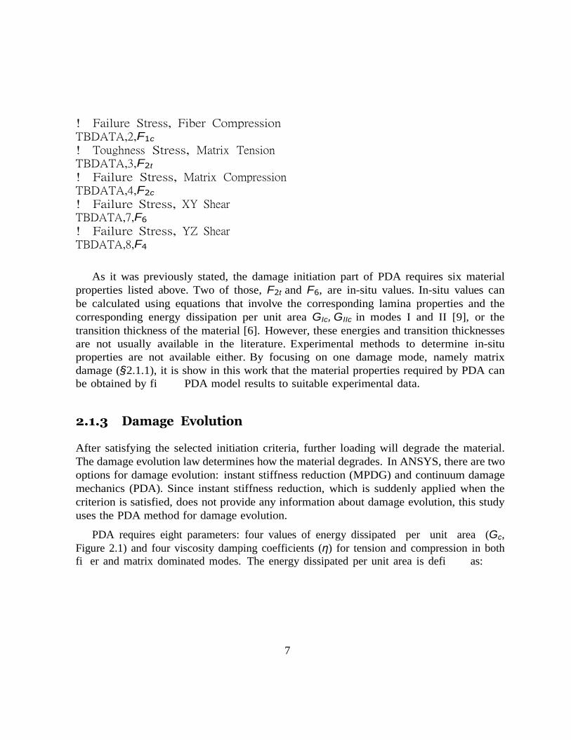
PDA requires eight parameters: four values of energy dissipated per unit area (Gc,
Figure 2.1) and four viscosity damping coefficients (η) for tension and compression in both
fi er and matrix dominated modes. The energy dissipated per unit area is defi as:
8
f
uf
di
Figure 2.1: Equivalent stress σe vs. equivalent displacement ue.
where:
r ue
G = 0
σedue (2.5)
σe = is the equivalent stress. For simple uniaxial stress state, the equivalent stress is the
actual stress. For complex stress state, the equivalent stresses and strains are calculated
based on Hashin’s damage initiation criteria.
ue = is the equivalent displacement. For simple uniaxial stress state, ue = E × Lc, and
Lc is the length of the element in the stress direction.
e = is the ultimate equivalent displacement, where total material stiffness is lost for
the specific mode.
Viscous damping coefficients η are also specified respectively for each of the damage
modes. For a specific damage mode, the damage evolution is regularized as follows:
η ∆t
t+∆t = η + ∆t
dt + η + ∆t
dt+∆t (2.6)
di i
where:
t+∆t = Regularized damage variable at current time. dt+∆t is used for material degra-
dation
9
di
c
c
c
c
c
t = Regularized damage variable at previous time.
dt+∆t = Un-regularized current damage variable
The command for defi damage evolution in APDL is TB,DMGE, as shown below.
! Damage Evolution with CDM Method TB,DMGE,1,1,8,CDM TBTEMP,0
! Fracture Toughness, Fiber Tensile TBDATA,1,Gft
! Viscosity Damping Coefficient, Fiber Tensile TBDATA,2, ηft
! Fracture Toughness, Fiber Compressive TBDATA,3,Gfc1E6 ! Viscosity Damping Coefficient, Fiber Compressive TBDATA,4, ηfc
! Fracture Toughness, Matrix Tensile TBDATA,5,Gtm
! Viscosity Damping Coefficient, Matrix Tensile TBDATA,6, ηmt
! Fracture Toughness, Matrix Compressive TBDATA,7,Gmc
! Viscosity Damping Coefficient, Matrix Compressive TBDATA,8, ηmc
As it was previously stated, the damage evolution part of PDA requires four material
properties, i.e., four values of Gc (eq. 2.5), that are not available in the literature. Ex-
perimental methods to determine these properties are not available either. By focusing
on one damage mode, namely matrix/shear damage (§2.1.1), it is show in this work that
the material properties in question (F2t,F6,and Gmt) can be obtained by fi the model
results to suitable experimental data.
10
c
c
i
i
c
2.2 PDA Design of Experiments The next step is to use design of experiments (DoE) and optimization to adjust the values
of F2t, F6, and Gmt so that the PDA prediction closely approximates the experimental
data.
First we use DoE to identify the laminates that are most sensitive to each parameter.
The focus at this point is to identify the minimum number of experiments that are needed
to adjust the parameters. In this way, additional experiments conducted with diff t
laminate stacking sequences (LSS) are not used to adjust parameters but to asses the
quality of the predictions.
In principle, the DoE technique is used to fi the location of sampling points in a way
that the space of random input parameters X = {F2t, F6, Gtm} is explored in the most
efficient way and that the output function D can be obtained with the minimum number
of sampling points. In this study the output function (also called objective function) is the
error between the predictions and the experimental data. Given N experimental values of
laminate modulus E(Ei), where E is the strain applied to the laminate, and i = 1 . . . N , the
error is defi as
1 N
E ANSY S Experimental
\2 D =
−
E (2.7)
N i=1
E� E=E E�
E=E
where E and E� are laminate elastic modulus for damaged and undamaged laminate, re-
spectively, and N is the number of experimental data points.
DoE tools can be found in ANSYS Workbench in the Design Explorer (DE) module,
which includes also Direct Optimization (DO), Parameters Correlation, Response Surface
(RS), Response Surface Optimization, and Six Sigma Analysis.
Let’s denote the input parameters by the array X = {F2t, F6, Gtm}. In this case, the
output function D = D(X) can be calculated by evaluation of eq. (2.7) through execution
of the fi element analysis (FEA) code for N values of strain. Each FEA analysis is
controlled by the APDL script, which calls for the evaluation of the non-linear response of
the damaging laminate for each value of strain, with parameters X. If the mesh is refined,
these evaluations could be computationally intensive.
An alternative to direct evaluation of the output function is to approximate it with
a multivariate quadratic polynomial. The approximation is called response surface (RS).
11
It can be constructed with only few actual evaluations of the output by choosing a small
number of sampling points for the input. The sampling points are chosen using Design of
Experiments (DoE) theory. The number of evaluations needed to construct the response
surface (RS) and for direct optimization (DO) are shown in Table 2.1.
# of inputs
Inputs
# of evaluations
RS DO (Screening)
DO (Adaptive Single-Objective)
1 F6 5 100 7
2 F6, Gmt
c 9 100 33
3 F2t, F6, Gmt
c 15 100 14
Table 2.1: Number of FEA evaluations used (a) to construct the response surface (RS)
and (b) to adjust the input parameters by direct optimization (DO).
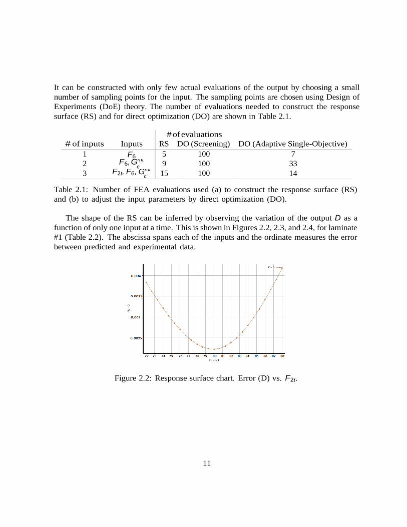
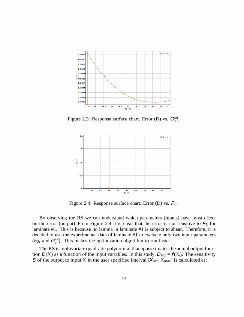
The shape of the RS can be inferred by observing the variation of the output D as a
function of only one input at a time. This is shown in Figures 2.2, 2.3, and 2.4, for laminate
#1 (Table 2.2). The abscissa spans each of the inputs and the ordinate measures the error
between predicted and experimental data.
Figure 2.2: Response surface chart. Error (D) vs. F2t.
12
c
c
Figure 2.3: Response surface chart. Error (D) vs. Gmt.
Figure 2.4: Response surface chart. Error (D) vs. F6.
By observing the RS we can understand which parameters (inputs) have most effect
on the error (output). From Figure 2.4 it is clear that the error is not sensitive to F6 for
laminate #1. This is because no lamina in laminate #1 is subject to shear. Therefore, it is
decided to use the experimental data of laminate #1 to evaluate only two input parameters
(F2t and Gmt). This makes the optimization algorithm to run faster.
The RS is multivariate quadratic polynomial that approximates the actual output func-
tion D(X) as a function of the input variables. In this study, DRS = f (Xi). The sensitivity
S of the output to input X in the user specified interval [Xmin, Xmax] is calculated as:
13
Laminate # LSS
1 [02/904]S
2 [±15/904]S
3 [±30/904]S
4 [±40/904]S
8 [0/ ± 404/01/2]S
9 [0/ ± 254/01/2]S
Table 2.2: Laminate stacking sequence for all laminates for which experimental data is
available.
S = max(D) − min(D)
average(D)
(2.8)
and tabulated in Table 2.3 for laminate # 1. Note that the sensitivity can be calculated
from the error evaluated directly from FEA analysis or from the RS. The later is much
more expedient than the former, as it can be seen in Table 2.1.
Input range Error D Sensitivity
Input min(Input) max(Input) min(D) max(D) ave(D) S F2t 72 88 0.0022 0.0041 0.00297 0.64
Gmt c 22.5 27.5 0.0031 0.0020 0.0026 -0.42
F6 50 88 0.076 0.102 0.093 -0.28
Table 2.3: Sensitivity S of the output (error) to each input (parameter). First two rows
refer to laminate #1 and last row to laminate #8.
The charts in Figures 2.2–2.4 are drawn for the input ranges given in Table 2.3. It is
convenient to compare all of them in one chart (Figure), where the input range has been
normalized to the interval [0–1].
2.3 Methodology The input parameters can be adjusted with any mesh and any type of elements that
represent the gauge section of the specimen, or a single element to represent a single
material point of the specimen. For expediency, a single linear element (SHELL 181) is
used in this study.
14
c
2.3.1 APDL
The APDL script is used to specify the mesh, boundary conditions, and the strain applied to
the laminate. The later is specified by imposing a specified displacement. Incrementation
of the applied displacement is implemented to mimic the experimental data, which is
available for a fi set of values of applied strain.
The APDL script is used also to specify the elastic properties (with MP command,
Table 2.4), the laminate stacking sequence (with SECDATA command, Table 2.2), the
material strengths (with TB command, Table 2.4). In Table 2.4, the material strengths
that are to be adjusted (F2t, F6) are simply initial (guess) values for the optimization.
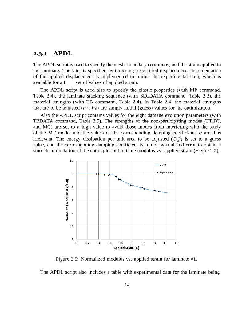
Also the APDL script contains values for the eight damage evolution parameters (with
TBDATA command, Table 2.5). The strengths of the non-participating modes (FT,FC,
and MC) are set to a high value to avoid those modes from interfering with the study
of the MT mode, and the values of the corresponding damping coefficients η are thus
irrelevant. The energy dissipation per unit area to be adjusted (Gmt) is set to a guess
value, and the corresponding damping coefficient is found by trial and error to obtain a
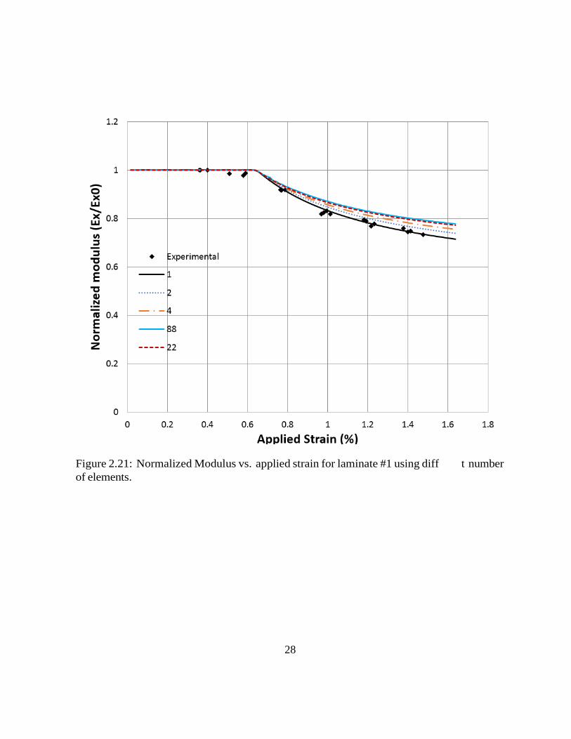
smooth computation of the entire plot of laminate modulus vs. applied strain (Figure 2.5).
Figure 2.5: Normalized modulus vs. applied strain for laminate #1.
The APDL script also includes a table with experimental data for the laminate being
15
Gt
Gc
Gc
Gtm
ηc
ηt
ηc
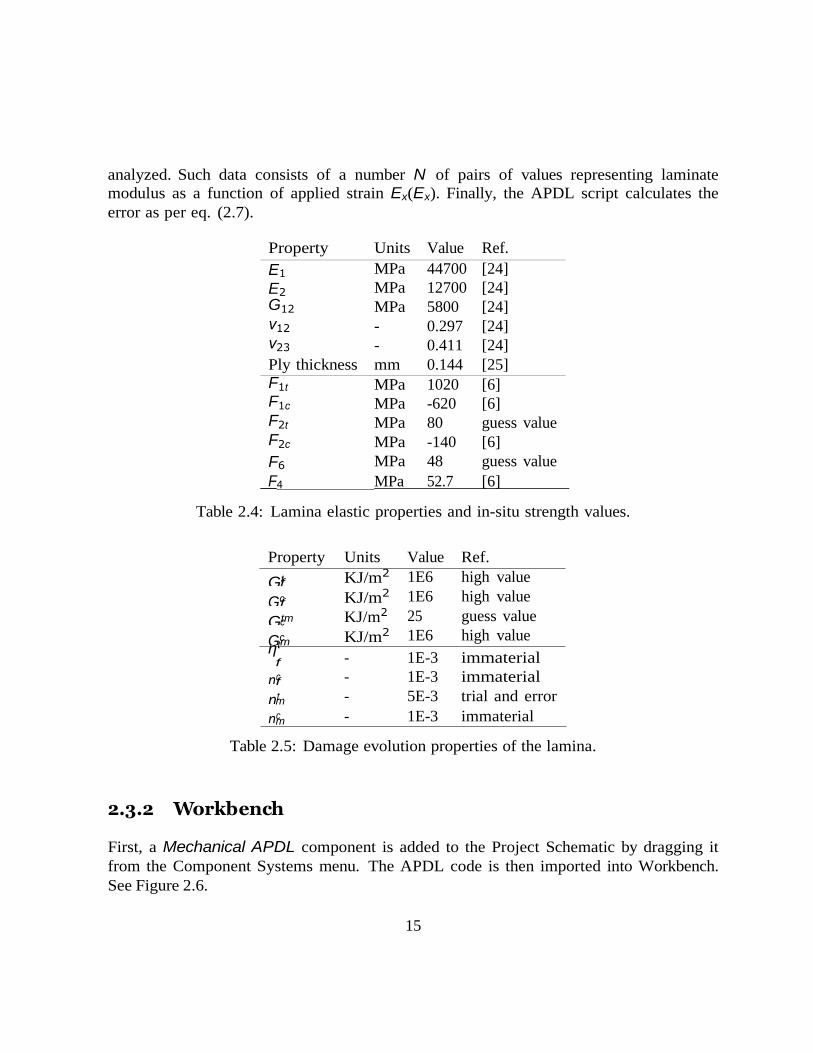
analyzed. Such data consists of a number N of pairs of values representing laminate
modulus as a function of applied strain Ex(Ex). Finally, the APDL script calculates the
error as per eq. (2.7).
Property Units Value Ref.
E1 MPa 44700 [24]
E2 MPa 12700 [24] G12 MPa 5800 [24] ν12 - 0.297 [24] ν23 - 0.411 [24]
Ply thickness mm 0.144 [25]
F1t MPa 1020 [6] F1c MPa -620 [6] F2t MPa 80 guess value F2c MPa -140 [6]
F6 MPa 48 guess value
F4 MPa 52.7 [6]
Table 2.4: Lamina elastic properties and in-situ strength values.
Property Units Value Ref.
f KJ/m2
f KJ/m2
c KJ/m2
m KJ/m2
ηt
1E6 high value
1E6 high value
25 guess value
1E6 high value
f - 1E-3 immaterial
f - 1E-3 immaterial
m - 5E-3 trial and error
m - 1E-3 immaterial
Table 2.5: Damage evolution properties of the lamina.
2.3.2 Workbench
First, a Mechanical APDL component is added to the Project Schematic by dragging it
from the Component Systems menu. The APDL code is then imported into Workbench.
See Figure 2.6.
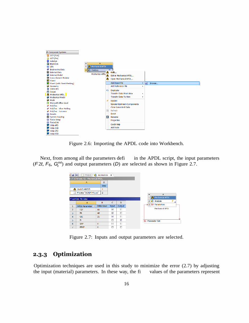
c
Figure 2.6: Importing the APDL code into Workbench.
Next, from among all the parameters defi in the APDL script, the input parameters
(F 2t, F6, Gmt) and output parameters (D) are selected as shown in Figure 2.7.
Figure 2.7: Inputs and output parameters are selected.
2.3.3 Optimization
Optimization techniques are used in this study to minimize the error (2.7) by adjusting
the input (material) parameters. In these way, the fi values of the parameters represent
16
17
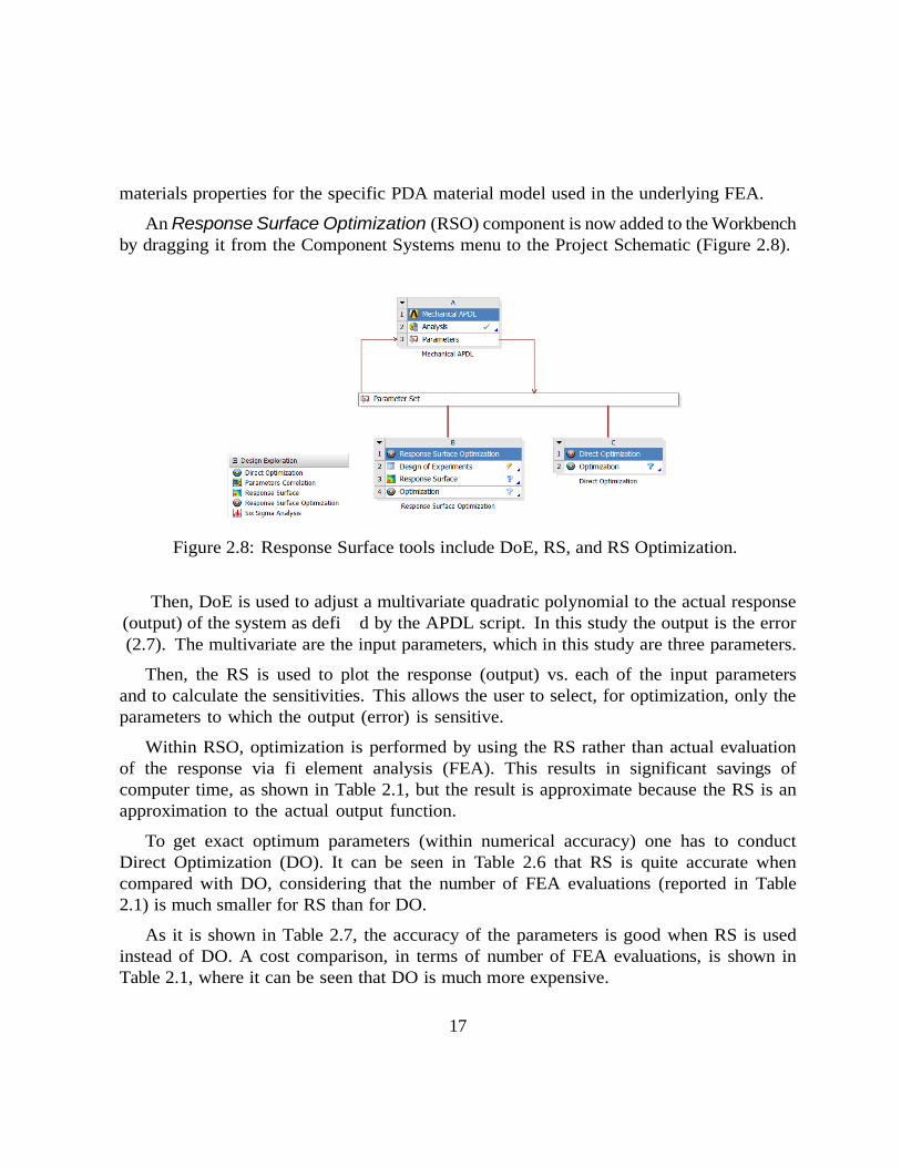
materials properties for the specific PDA material model used in the underlying FEA.
An Response Surface Optimization (RSO) component is now added to the Workbench
by dragging it from the Component Systems menu to the Project Schematic (Figure 2.8).
Figure 2.8: Response Surface tools include DoE, RS, and RS Optimization.
Then, DoE is used to adjust a multivariate quadratic polynomial to the actual response
(output) of the system as defi d by the APDL script. In this study the output is the error
(2.7). The multivariate are the input parameters, which in this study are three parameters.
Then, the RS is used to plot the response (output) vs. each of the input parameters
and to calculate the sensitivities. This allows the user to select, for optimization, only the
parameters to which the output (error) is sensitive.
Within RSO, optimization is performed by using the RS rather than actual evaluation
of the response via fi element analysis (FEA). This results in significant savings of
computer time, as shown in Table 2.1, but the result is approximate because the RS is an
approximation to the actual output function.
To get exact optimum parameters (within numerical accuracy) one has to conduct
Direct Optimization (DO). It can be seen in Table 2.6 that RS is quite accurate when
compared with DO, considering that the number of FEA evaluations (reported in Table
2.1) is much smaller for RS than for DO.
As it is shown in Table 2.7, the accuracy of the parameters is good when RS is used
instead of DO. A cost comparison, in terms of number of FEA evaluations, is shown in
Table 2.1, where it can be seen that DO is much more expensive.
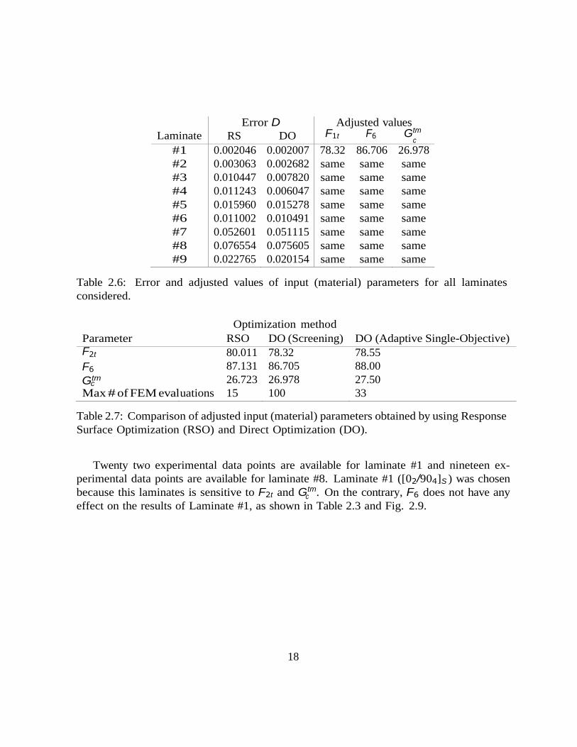
18
c
Laminate
Error D
RS DO
Adjusted values F1t F6 Gtm
c
#1 0.002046 0.002007 78.32 86.706 26.978
#2 0.003063 0.002682 same same same
#3 0.010447 0.007820 same same same
#4 0.011243 0.006047 same same same
#5 0.015960 0.015278 same same same
#6 0.011002 0.010491 same same same
#7 0.052601 0.051115 same same same
#8 0.076554 0.075605 same same same
#9 0.022765 0.020154 same same same
Table 2.6: Error and adjusted values of input (material) parameters for all laminates
considered.
Optimization method
Parameter RSO DO (Screening) DO (Adaptive Single-Objective)
F2t 80.011 78.32 78.55
F6 87.131 86.705 88.00
Gtm c 26.723 26.978 27.50
Max # of FEM eval uations 15 100 33
Table 2.7: Comparison of adjusted input (material) parameters obtained by using Response
Surface Optimization (RSO) and Direct Optimization (DO).
Twenty two experimental data points are available for laminate #1 and nineteen ex-
perimental data points are available for laminate #8. Laminate #1 ([02/904]S ) was chosen
because this laminates is sensitive to F2t and Gtm. On the contrary, F6 does not have any
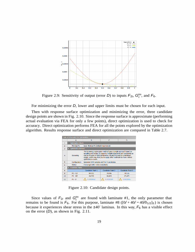
effect on the results of Laminate #1, as shown in Table 2.3 and Fig. 2.9.
19
c
c
Figure 2.9: Sensitivity of output (error D) to inputs F2t, Gtm, and F6.
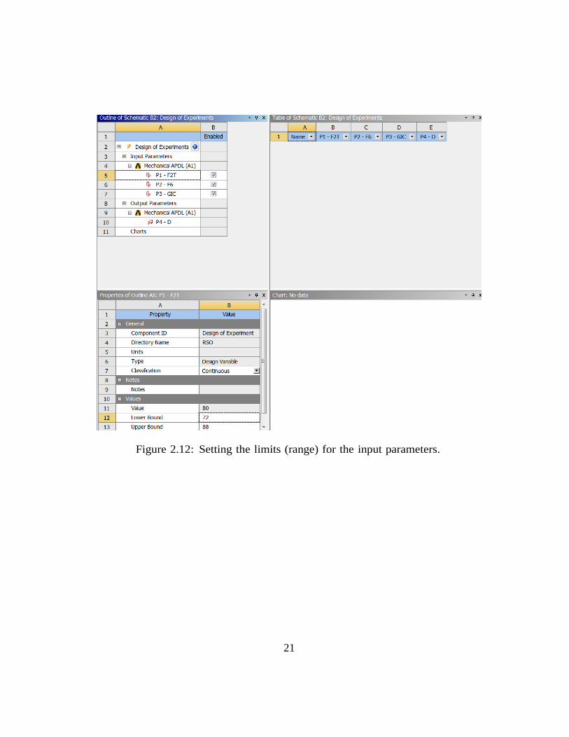
For minimizing the error D, lower and upper limits must be chosen for each input.
Then with response surface optimization and minimizing the error, three candidate
design points are shown in Fig. 2.10. Since the response surface is approximate (performing
actual evaluation via FEA for only a few points), direct optimization is used to check for
accuracy. Direct optimization performs FEA for all the points explored by the optimization
algorithm. Results response surface and direct optimization are compared in Table 2.7.
Figure 2.10: Candidate design points.
Since values of F2t and Gtm are found with laminate #1, the only parameter that
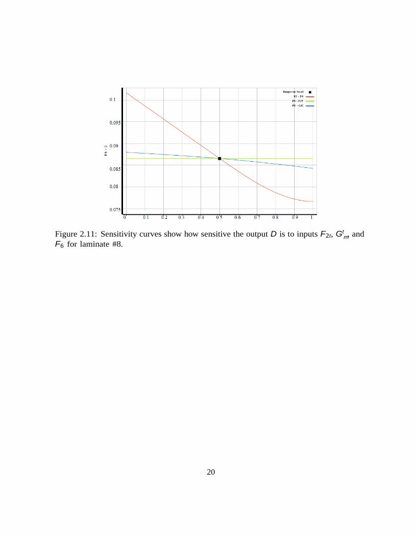
remains to be found is F6. For this purpose, laminate #8 ([0/ + 40/ − 40/01/2]S ) is chosen
because it experiences shear stress in the ±40◦ laminas. In this way, F6 has a visible effect on the error (D), as shown in Fig. 2.11.
20
m
Figure 2.11: Sensitivity curves show how sensitive the output D is to inputs F2t, Gt , and
F6 for laminate #8.
21
Figure 2.12: Setting the limits (range) for the input parameters.
22
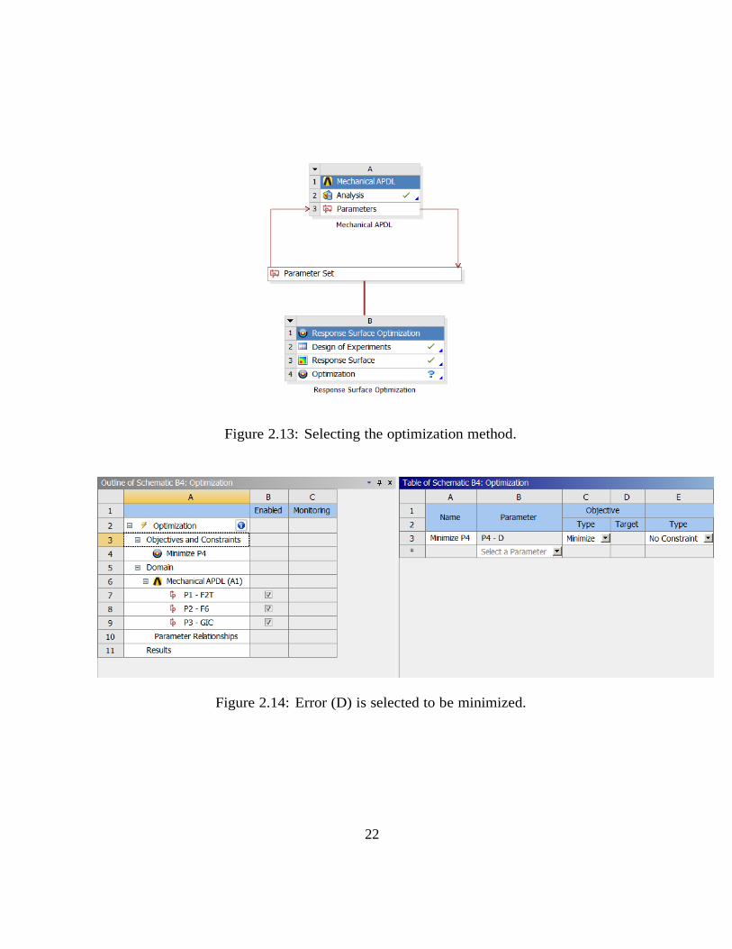
Figure 2.13: Selecting the optimization method.
Figure 2.14: Error (D) is selected to be minimized.
23
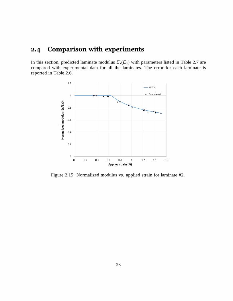
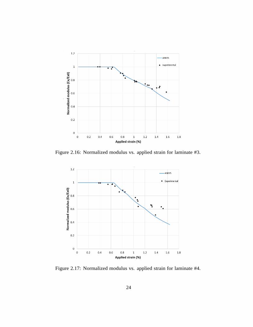
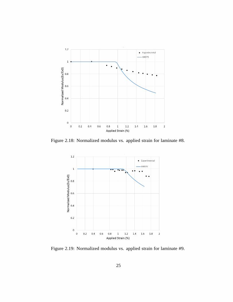
2.4 Comparison with experiments In this section, predicted laminate modulus Ex(Ex) with parameters listed in Table 2.7 are
compared with experimental data for all the laminates. The error for each laminate is
reported in Table 2.6.
Figure 2.15: Normalized modulus vs. applied strain for laminate #2.
24
Figure 2.16: Normalized modulus vs. applied strain for laminate #3.
Figure 2.17: Normalized modulus vs. applied strain for laminate #4.
25
Figure 2.18: Normalized modulus vs. applied strain for laminate #8.
Figure 2.19: Normalized modulus vs. applied strain for laminate #9.
26
As shown in Fig. 2.18-2.19, ANSYS PDA cannot predict the damage behavior of
laminate #8 and laminate #9 as good as damage behavior of laminate #1 to #5, it is
because latter laminates do not have to tolerate shear stress due to the angle of fi ers in
them (all of them have 90 degree laminas) but laminate #8 and #9 should tolerate shear
stress.
2.5 Mesh sensitivity Mesh sensitivity refers to how much the solution changes with mesh density, number of
elements, or number of nodes used to discretize the problem under study. There are two
sources of mesh sensitivity. The most obvious is type I sensitivity, where the quality of
the solution, particularly stress and strain gradients, depends on mesh density; the fi
the mesh, the better the accuracy of the solution. Assuming that the mesh is refined
enough to capture stress/strain gradients satisfactorily, type II sensitivity may come from
the constitutive model used. When the material response is non-linear, the constitutive
model calculates the stress for a given strain and updates one or more state variables to
keep track of the history of the material state. Ideally, the response of the constitutive
model should be independent of the mesh. To isolate the two sources of mesh dependency,
it is customary to test the software with examples for which the strain fi is uniform in
the domain regardless of mesh density. The physical tensile test in this study experiences
uniform strain everywhere in the rectangular domain representing the gage section of the
specimen. Under these conditions, the reaction force calculated by FEA for a given applied
strain should be independent of the mesh. There is no type I mesh sensitivity in the
calculation of displacement and strain because the strain is uniform in the entire domain.
But the reaction force depends on the accuracy of the constitutive model. It can be seen
in Fig. 2.20 that PDA is mesh sensitive.
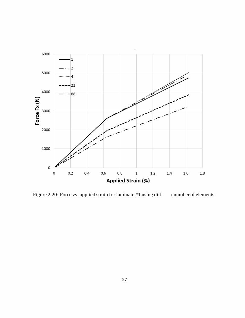
27
Figure 2.20: Force vs. applied strain for laminate #1 using diff t number of elements.
28
Figure 2.21: Normalized Modulus vs. applied strain for laminate #1 using diff t number
of elements.
29
Chapter 3 Discrete Damage Mechanics (DDM)
DDM [4] is a constitutive modeler that is mesh independent, so DDM does not require the
user to choose a characteristic length as in the PDA chapter. Only two material parame-
ters, the fracture toughness in modes I and II, are required to predict both initiation and
evolution of transverse and shear damage. Since transverse and shear strengths are not
used to predict damage initiation, but rather fracture toughness is used, DDM automati-
cally accounts for in-situ effects. No additional parameters are required to predict damage
evolution.
DDM is available to be used in conjunction with commercial FEA environments such as
ANSYS/Mechanical [1], in the form USERMAT [5]. Therefore, the objective of this chapter
is to propose a methodology to determine values for the material properties required by
the DDM model. In this work, the values for the parameters are found using available
experimental data and a rational procedure. Once values are found, the DDM model is
applied for predicting other, independent results, and conclusions are drawn about the
applicability of the model.
An standard test method exist for measuring interlaminar fracture toughness in mode
I (ASTM D5528) and a proposed method exists for interlaminar mode II [21]. However,
no standards exist for intralaminar mode I and mode II. Intralaminar damage, which is
the subject of this thesis, is not the same as interlaminar delamination. Therefore, the
interlaminar properties cannot be used for predicting intralaminar damage. Instead, the
properties can be evaluated as explained in this thesis.
30
3.1 Discrete Damage Mechanics By increasing the strain Ex, DDM updates the state variables (crack density λ), and calcu-
late the shell stress resultants N, M, and tangent stiffness matrix AT , BT , DT as functions
of crack density. The crack density λ is an array containing the crack density for all laminas
at an integration point of the shell element. Since fracture toughness is used to predict
damage initiation for DDM model, DDM does not need in-situ correction of strength.
This study shows how to use available data to infer the material properties required
by DDM model. Specifically, the main purpose of this study is to fi the critical value
of the energy release rate (ERR) in first mode GIc and critical value of ERR in second
mode II GIIc for the material system (composite lamina) that can be used in DDM to
predict damage initiation and evolution of laminated composite structures built with the
same material system.
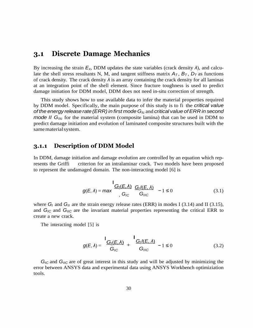
3.1.1 Description of DDM Model In DDM, damage initiation and damage evolution are controlled by an equation which rep-
resents the Griffi criterion for an intralaminar crack. Two models have been proposed
to represent the undamaged domain. The non-interacting model [6] is
I GI (E, λ)
g(E, λ) = max , GIC
GI I(E, λ)
GIIC
− 1 ≤ 0 (3.1)
where GI and GII are the strain energy release rates (ERR) in modes I (3.14) and II (3.15),
and GIC and GIIC are the invariant material properties representing the critical ERR to
create a new crack.
The interacting model [5] is
g(E, λ) =
I GI (E, λ)
GIC
I GI I(E, λ)
+ GIIC
− 1 ≤ 0 (3.2)
GIC and GIIC are of great interest in this study and will be adjusted by minimizing the
error between ANSYS data and experimental data using ANSYS Workbench optimiziation
tools.
i =
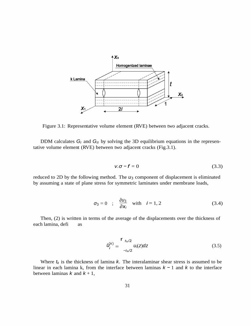
Figure 3.1: Representative volume element (RVE) between two adjacent cracks.
DDM calculates GI and GII by solving the 3D equilibrium equations in the represen-
tative volume element (RVE) between two adjacent cracks (Fig.3.1).
v.σ − f = 0 (3.3)
reduced to 2D by the following method. The u3 component of displacement is eliminated
by assuming a state of plane stress for symmetric laminates under membrane loads,
σ3 = 0 ; ∂u3
∂xi with i = 1, 2 (3.4)
Then, (2) is written in terms of the average of the displacements over the thickness of
each lamina, defi as
u(k) r tk /2
−tk /2
ui(z)dz (3.5)
Where tk is the thickness of lamina k. The interalaminar shear stress is assumed to be
linear in each lamina k, from the interface between laminas k − 1 and k to the interface
between laminas k and k + 1,
31
32
3
3
σ(c)
τ (k)
k−1,k
k,k+1
k−1,k x3
— xk−1,k
j3 (x3) = τj3 + τj3 − τj3 ; j = 1, 2 (3.6)
tk
Where x3 is the coordinate indirection of the thickness of laminate, and xk−1,k is the
coordinate of the interface between laminas k − 1 and k. Therefore, the 3D equilibrium
equations (2) reduce to a 2D second order partial diff tial equations (PDE) as a function
of average displacements, with two equations per lamina.
As shown in Fig. 3.1 the crack density is inversely proportional to the length 2l of
representative volume element (RVE).
1 λ = (3.7)
2l
AS seen in (6) the crack density in the DDM model is calculated by the length of the
RVE. Since, the RVE is independent of the element size and type, the constitutive model is
objective without needing a characteristic length such as element length in ANSYS PDA,
so DDM model is mech insensitive that is shown in Fig. 3.30.
The PDE system is complemented by the following boundary conditions. The surface
of the cracks in lamina c, located at x = ±l, are free boundaries, and thus subject to zero
stress.
r 1/2
−1/2
j (x1, l)dx1 = 0 ; j = 2, 6 (3.8)
All laminas except the cracking lamina (c), undergo the same displacement at the bound-
aries (−l, l) when subjected to a membrane state of strain. Taking an arbitrary lamina
r /= c as a reference, the other displacements are
u(m) (r)
j (x1, ±l) /= uj (x1, ±l) ; m /= k ; j = 1, 2 (3.9)
Finally, the stress resultant from the internal stress equilibrates the applied load. In the
parallel direction to the surface of the cracks (fiber direction x1) the load is supported by
all the laminas in the laminate,
33
σ(k)
σ(m)
2
1 N r l 1
tk
2l
k=1
1 ( , x2)dx2 = N1 (3.10) −l
but, in the normal direction to the crack surface (x2 direction), only the intact laminas
m /= c carry loads (normal and shear)
r 1/2
j (x1, l)dx1 = Nj ; j = 2, 6 (3.11)
m/=k −1/2
The solution of the PDE system results in fi ding the displacements in all laminas u(k),
and by diff tiation, the strains in all laminas. Then, the S matrix of the laminate is
calculated by solving three load cases
1
1
1
aN/t =
0
; bN/t =
0
; cN/t =
0
; ∆T = 0 (3.12)
0
0
0
where t is the thickness of the laminate. Since the three applied stress states are unit
values, for each case, a, b, c, the volume average of the strain represents one column in the
laminate compliance matrix
aEx
bEx cEx
S = aEy bEy cEy (3.13)
aλxy bλxy
cλxy
Next, the laminate inplane stiffness Q = A/t in the coordinate system of lamina k is
Q = S−1 (3.14)
34
}
I 2∆A
2 2 2j j j
II 2∆A
6 6 6j j j
∆λ = −
The degraded CTE of the laminate {αx, αy, αxy T
are given by the values {Ex, Ey, λxy}T
obtained for the case with loading N = {0, 0, 0}T and ∆T = 1. Then, the ERR in fracture
modes I and II are calculated as follows
G = −VRV E
(E − α ∆T )∆Q (E − α ∆T ) ; opening mode (3.15)
G = −
VRV E (E − α ∆T )∆Q (E − α ∆T ) ; shearing mode (3.16)
Tearing mode III does not occur because out of plane displacements of the lips of the
crack are constrained by the adjacent laminas in the laminate. The crack density is treated
as a continuous function, rather than a discrete function. Thus, the crack density is found
using a return mapping algorithm (RMA) to satisfy g = 0 in (1), as follows
gk
k ∂gk
∂λ
(3.17)
3.2 DDM Design of Experiments The next step is to use the design of experiments (DoE) and optimization to adjust the
values of GIc and GIIc so that the DDM prediction closely approximates the experimental
data.
First, we use DoE to identify the laminates that are most sensitive to each parameter.
The focus at this point is to determine the minimum number of experiments that are needed
to adjust the parameters. In this way, additional experiments conducted with diff t
laminate stacking sequences (LSS) are not used to adjust parameters but to assess the
quality of the predictions.
In principle, the DoE technique is used to fi the location of sampling points in a
way that the space of random input parameters X = {GIc, GIIc} is explored in the most
efficient way and that the output function D can be obtained with the minimum number
of sampling points. In this study, the output function (also called objective function) is the
error between the predictions and the experimental data. Given N experimental values of
laminate modulus E(Ei), where E is the strain applied to the laminate, and i = 1 . . . N , the
error is defi as
35
i
i
1 N
E ANSY S Experimental
\2 D =
−
E (3.18)
N i=1
E� E=E E�
E=E
where E and E� are laminate elastic modulus for damaged and undamaged laminate, re-
spectively, and N is the number of experimental data points.
DoE tools can be found in ANSYS Workbench in the Design Explorer (DE) module,
which includes also Direct Optimization (DO), Parameters Correlation, Response Surface
(RS), Response Surface Optimization, and Six Sigma Analysis.
Let’s denote the input parameters by the array X = {GIc, GIIc}. In this case, the
output function D = D(X) can be calculated by evaluation of eq. (3.18) through execution
of the fi element analysis (FEA) code for N values of strain. Each FEA analysis is
controlled by the APDL script, which calls for the evaluation of the non-linear response of
the damaging laminate for each value of strain, with parameters X. If the mesh is refined,
these evaluations could be computationally intensive.
An alternative to direct evaluation of the output function is to approximate it with
a multivariate quadratic polynomial. The approximation is called response surface (RS).
It can be constructed with only few actual evaluations of the output by choosing a small
number of sampling points for the input. The sampling points are chosen using Design of
Experiments (DoE) theory. The number of evaluations needed to construct the response
surface (RS) and for direct optimization (DO) are shown in Table 3.1.
# of inputs
Inputs
# of evaluations
Response Surface DO (Adaptive Single-Objective)
1 GIc 5 9
2 GIc, GIIc 9 21
Table 3.1: Number of FEA evaluations used (a) to construct the response surface (RS)
and (b) to adjust the input parameters by direct optimization (DO). Interacting equation
(3.2) is used.
The shape of the RS can be inferred by observing the variation of the output D as a
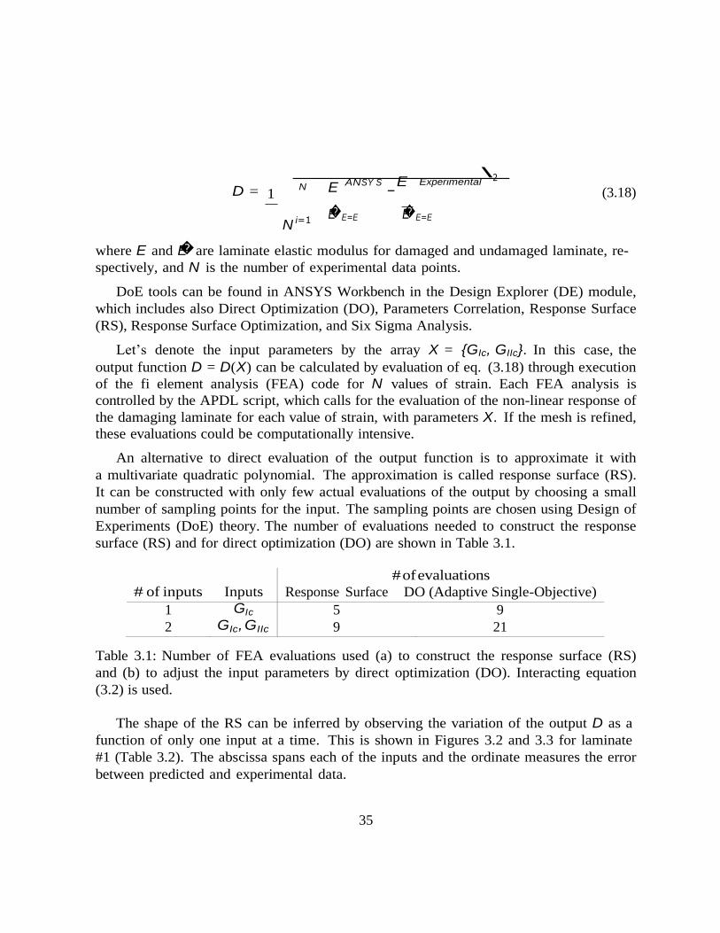
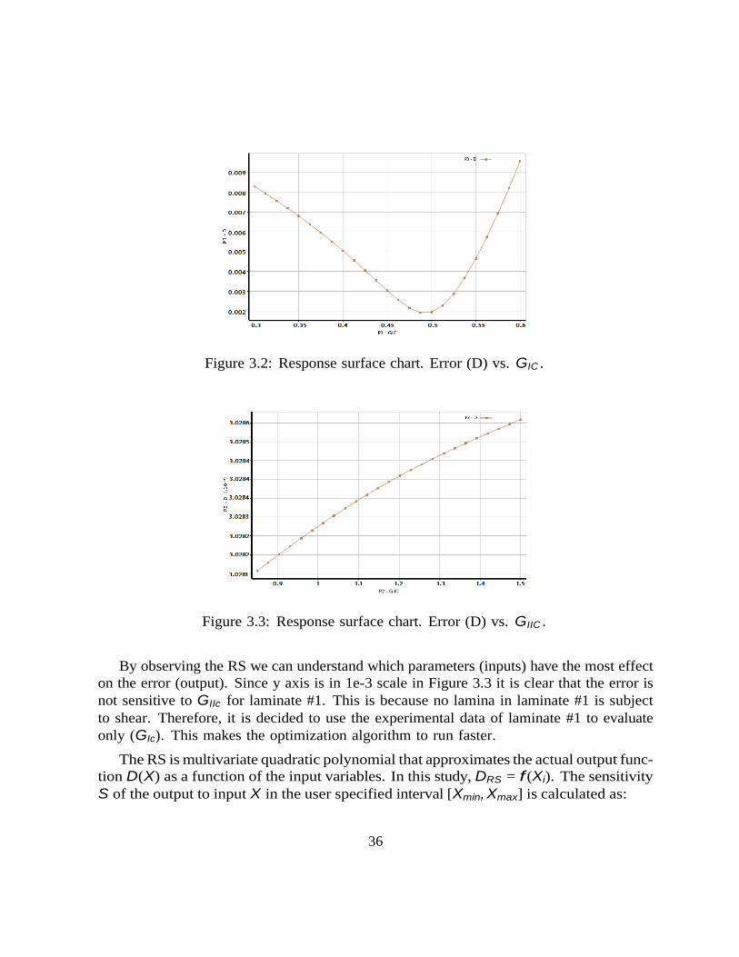
function of only one input at a time. This is shown in Figures 3.2 and 3.3 for laminate
#1 (Table 3.2). The abscissa spans each of the inputs and the ordinate measures the error
between predicted and experimental data.
36
Figure 3.2: Response surface chart. Error (D) vs. GIC .
Figure 3.3: Response surface chart. Error (D) vs. GIIC .
By observing the RS we can understand which parameters (inputs) have the most effect
on the error (output). Since y axis is in 1e-3 scale in Figure 3.3 it is clear that the error is
not sensitive to GIIc for laminate #1. This is because no lamina in laminate #1 is subject
to shear. Therefore, it is decided to use the experimental data of laminate #1 to evaluate
only (GIc). This makes the optimization algorithm to run faster.
The RS is multivariate quadratic polynomial that approximates the actual output func-
tion D(X) as a function of the input variables. In this study, DRS = f (Xi). The sensitivity
S of the output to input X in the user specified interval [Xmin, Xmax] is calculated as:
37
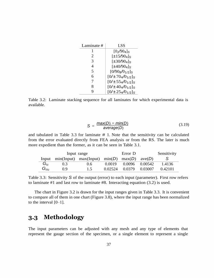
Laminate # LSS
1 [02/904]S
2 [±15/904]S
3 [±30/904]S
4 [±40/904]S
5 [0/908/01/2]S
6 [0/ ± 704/01/2]S
7 [0/ ± 554/01/2]S
8 [0/ ± 404/01/2]S
9 [0/ ± 254/01/2]S
Table 3.2: Laminate stacking sequence for all laminates for which experimental data is
available.
S = max(D) − min(D)
average(D)
(3.19)
and tabulated in Table 3.3 for laminate # 1. Note that the sensitivity can be calculated
from the error evaluated directly from FEA analysis or from the RS. The later is much
more expedient than the former, as it can be seen in Table 3.1.
Input range Error D Sensitivity
Input min(Input) max(Input) min(D) max(D) ave(D) S GIc 0.3 0.6 0.0019 0.0096 0.00542 1.4136 GIIc 0.9 1.5 0.02524 0.0379 0.03007 0.42101
Table 3.3: Sensitivity S of the output (error) to each input (parameter). First row refers
to laminate #1 and last row to laminate #8. Interacting equation (3.2) is used.
The chart in Figure 3.2 is drawn for the input ranges given in Table 3.3. It is convenient
to compare all of them in one chart (Figure 3.8), where the input range has been normalized
to the interval [0–1].
3.3 Methodology The input parameters can be adjusted with any mesh and any type of elements that
represent the gauge section of the specimen, or a single element to represent a single
38
material point of the specimen. For expediency, a single linear element (PLANE 182) is
used in this study.
3.3.1 APDL
The APDL script is used to call the usermaterial (DLL fi specify the mesh, boundary
conditions, and the strain applied to the laminate. The later is specified by imposing
a specified displacement. Incrementation of the applied displacement is implemented to
mimic the experimental data, which is available for a fi set of values of applied strain.
The APDL script is used also to specify the elastic properties (with TB command,
Table 3.4), the laminate stacking sequence (with TB command, Table 3.2), the the critical
ERRs (with TB command, Table 3.4). In Table 3.4, the critical ERRs that are adjusted
(GIc, GIIc) are simply initial (guess) values for the optimization.
Also the APDL script contains the geometry of the specimen. The dimensions of the
specimen are 20mm wide and 110mm free length. All the laminates considered for the
study are symmetric and balanced. Therefore a quarter of the specimen was used for the
analysis using symmetry boundary conditions and applying a uniform strain with imposed
displacements on one end of the specimen. A longitudinal displacement of 1.1mm was
applied to reach a strain of 2%.
39
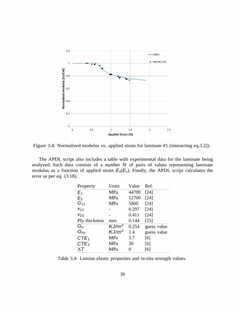
Figure 3.4: Normalized modulus vs. applied strain for laminate #1 (interacting eq.3.2]).
The APDL script also includes a table with experimental data for the laminate being
analyzed. Such data consists of a number N of pairs of values representing laminate
modulus as a function of applied strain Ex(Ex). Finally, the APDL script calculates the
error as per eq. (3.18).
Property Units Value Ref.
E1 MPa 44700 [24]
E2 MPa 12700 [24] G12 MPa 5800 [24] ν12 - 0.297 [24] ν23 - 0.411 [24]
Ply thickness mm 0.144 [25]
GIc KJ/m2 0.254 guess value
GIIc KJ/m2 1.4 guess value
CTE1 MPa 3.7 [6]
CTE2 MPa 30 [6]
∆T MPa 0 [6]
Table 3.4: Lamina elastic properties and in-situ strength values.
40
Gt
Gc
Gc
Gtm
ηc
ηt
ηc
c
Property Units Value Ref.
f KJ/m2
f KJ/m2
c KJ/m2
m KJ/m2
ηt
1E6 high value
1E6 high value
25 guess value
1E6 high value
f - 1E-3 immaterial
f - 1E-3 immaterial
m - 5E-3 trial and error
m - 1E-3 immaterial
Table 3.5: Damage evolution properties of the lamina.
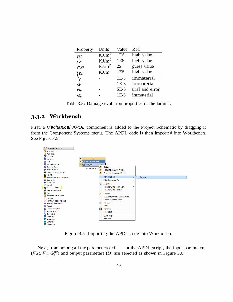
3.3.2 Workbench
First, a Mechanical APDL component is added to the Project Schematic by dragging it
from the Component Systems menu. The APDL code is then imported into Workbench.
See Figure 3.5.
Figure 3.5: Importing the APDL code into Workbench.
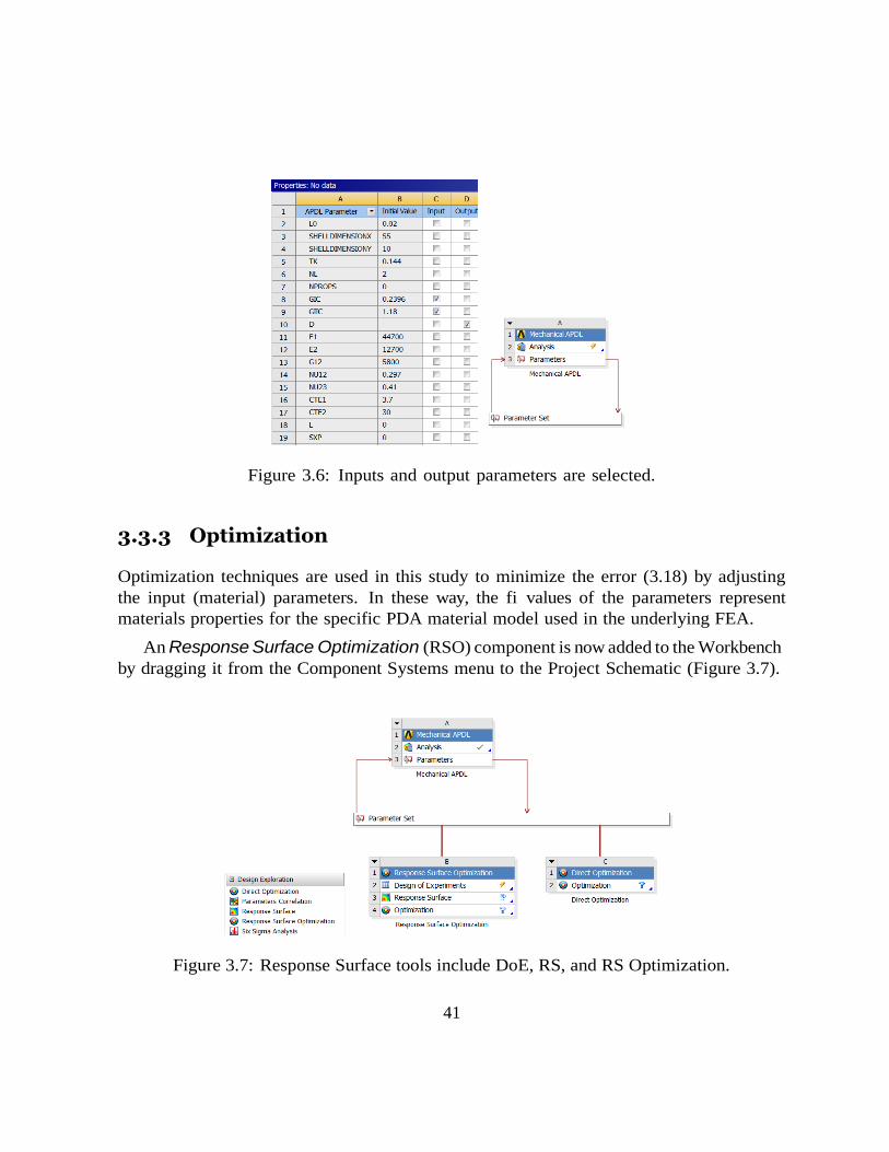
Next, from among all the parameters defi in the APDL script, the input parameters
(F 2t, F6, Gmt) and output parameters (D) are selected as shown in Figure 3.6.
41
Figure 3.6: Inputs and output parameters are selected.
3.3.3 Optimization Optimization techniques are used in this study to minimize the error (3.18) by adjusting
the input (material) parameters. In these way, the fi values of the parameters represent
materials properties for the specific PDA material model used in the underlying FEA.
An Response Surface Optimization (RSO) component is now added to the Workbench
by dragging it from the Component Systems menu to the Project Schematic (Figure 3.7).
Figure 3.7: Response Surface tools include DoE, RS, and RS Optimization.
42
Then, DoE is used to adjust a multivariate quadratic polynomial to the actual response
(output) of the system as defi by the APDL script. In this study the output is the
error (3.18). The multivariate are the input parameters, which in this chapter are two
parameters.
Then, the RS is used to plot the response (output) vs. each of the input parameters
and to calculate the sensitivities. This allows the user to select, for optimization, only the
parameters to which the output (error) is sensitive.
Within RSO, optimization is performed by using the RS rather than actual evaluation
of the response via fi element analysis (FEA). This results in significant savings of
computer time, as shown in Table 3.1, but the result is approximate because the RS is an
approximation to the actual output function.
To get exact optimum parameters (within numerical accuracy) one has to conduct
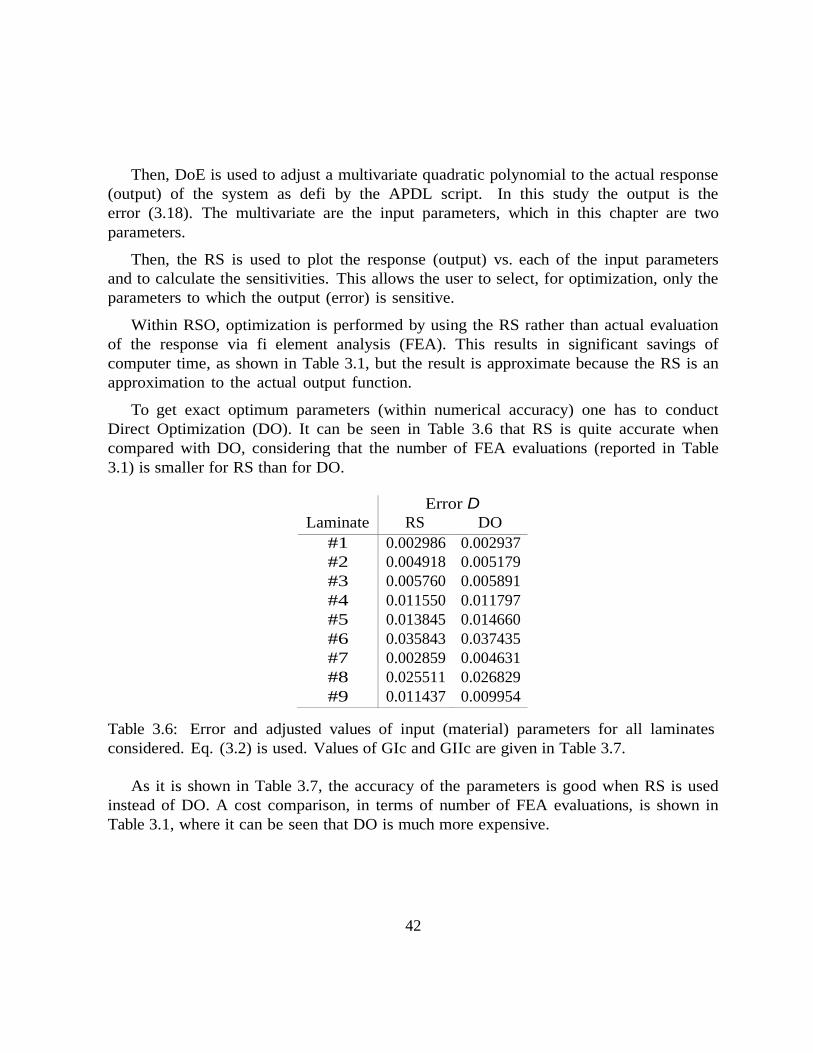
Direct Optimization (DO). It can be seen in Table 3.6 that RS is quite accurate when
compared with DO, considering that the number of FEA evaluations (reported in Table
3.1) is smaller for RS than for DO.
Laminate
Error D
RS DO
#1 0.002986 0.002937
#2 0.004918 0.005179
#3 0.005760 0.005891
#4 0.011550 0.011797
#5 0.013845 0.014660
#6 0.035843 0.037435
#7 0.002859 0.004631
#8 0.025511 0.026829
#9 0.011437 0.009954
Table 3.6: Error and adjusted values of input (material) parameters for all laminates
considered. Eq. (3.2) is used. Values of GIc and GIIc are given in Table 3.7.
As it is shown in Table 3.7, the accuracy of the parameters is good when RS is used
instead of DO. A cost comparison, in terms of number of FEA evaluations, is shown in
Table 3.1, where it can be seen that DO is much more expensive.
43
Optimization method
Parameter RSO (Response Surface) DO (Adaptive Single-Objective)
GIC 0.4285 0.437 GIIC 0.96597 1.0205
Max # of FEM evaluations 9 21
Table 3.7: Comparison of adjusted input (material) parameters obtained by using Response
Surface Optimization (RSO) and Direct Optimization (DO). Eq. (3.2) is used.
Twenty two experimental data points are available for laminate #1 and nineteen ex-
perimental data points are available for laminate #8. Laminate #1 ([02/904]S ) was chosen
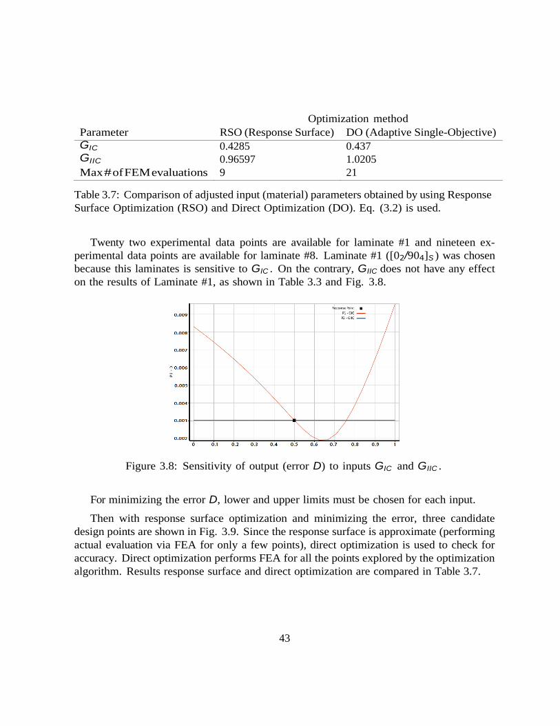
because this laminates is sensitive to GIC . On the contrary, GIIC does not have any effect
on the results of Laminate #1, as shown in Table 3.3 and Fig. 3.8.
Figure 3.8: Sensitivity of output (error D) to inputs GIC and GIIC .
For minimizing the error D, lower and upper limits must be chosen for each input.
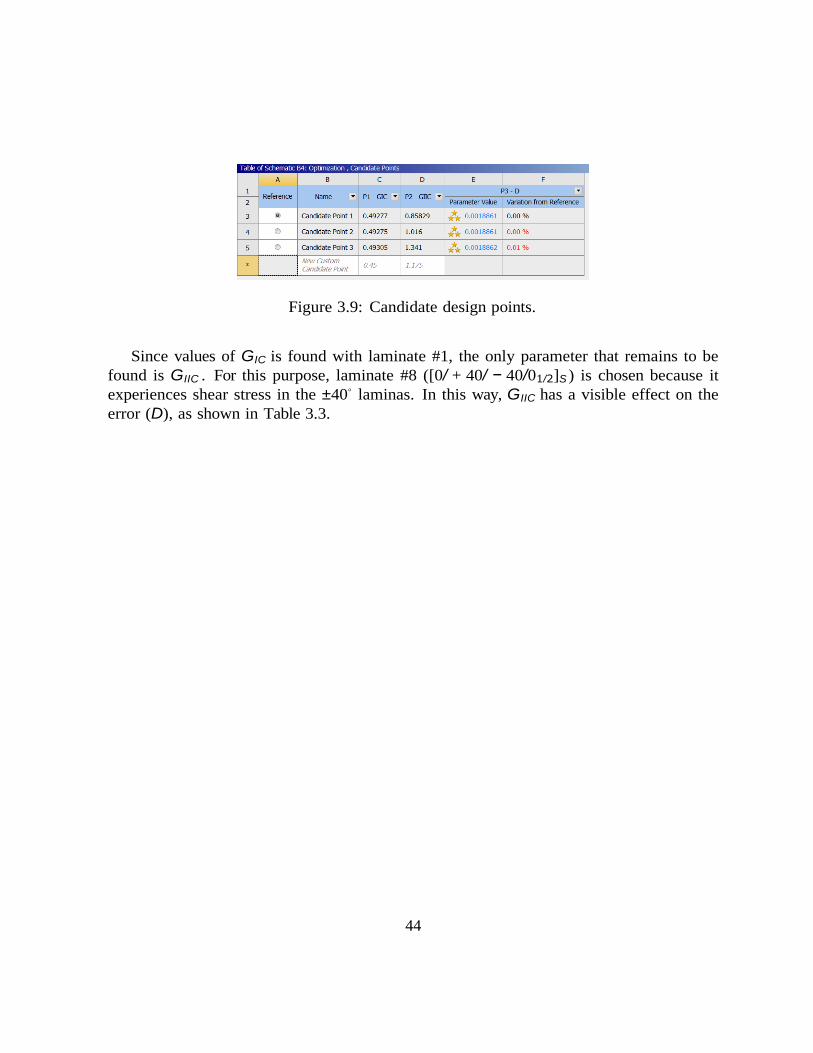
Then with response surface optimization and minimizing the error, three candidate
design points are shown in Fig. 3.9. Since the response surface is approximate (performing
actual evaluation via FEA for only a few points), direct optimization is used to check for
accuracy. Direct optimization performs FEA for all the points explored by the optimization
algorithm. Results response surface and direct optimization are compared in Table 3.7.
44
Figure 3.9: Candidate design points.
Since values of GIC is found with laminate #1, the only parameter that remains to be
found is GIIC . For this purpose, laminate #8 ([0/ + 40/ − 40/01/2]S ) is chosen because it
experiences shear stress in the ±40◦ laminas. In this way, GIIC has a visible effect on the
error (D), as shown in Table 3.3.
45
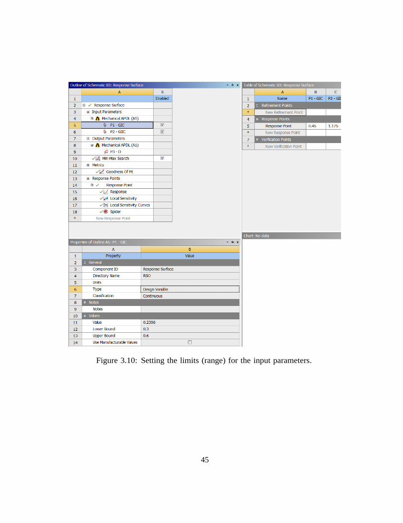
Figure 3.10: Setting the limits (range) for the input parameters.
46
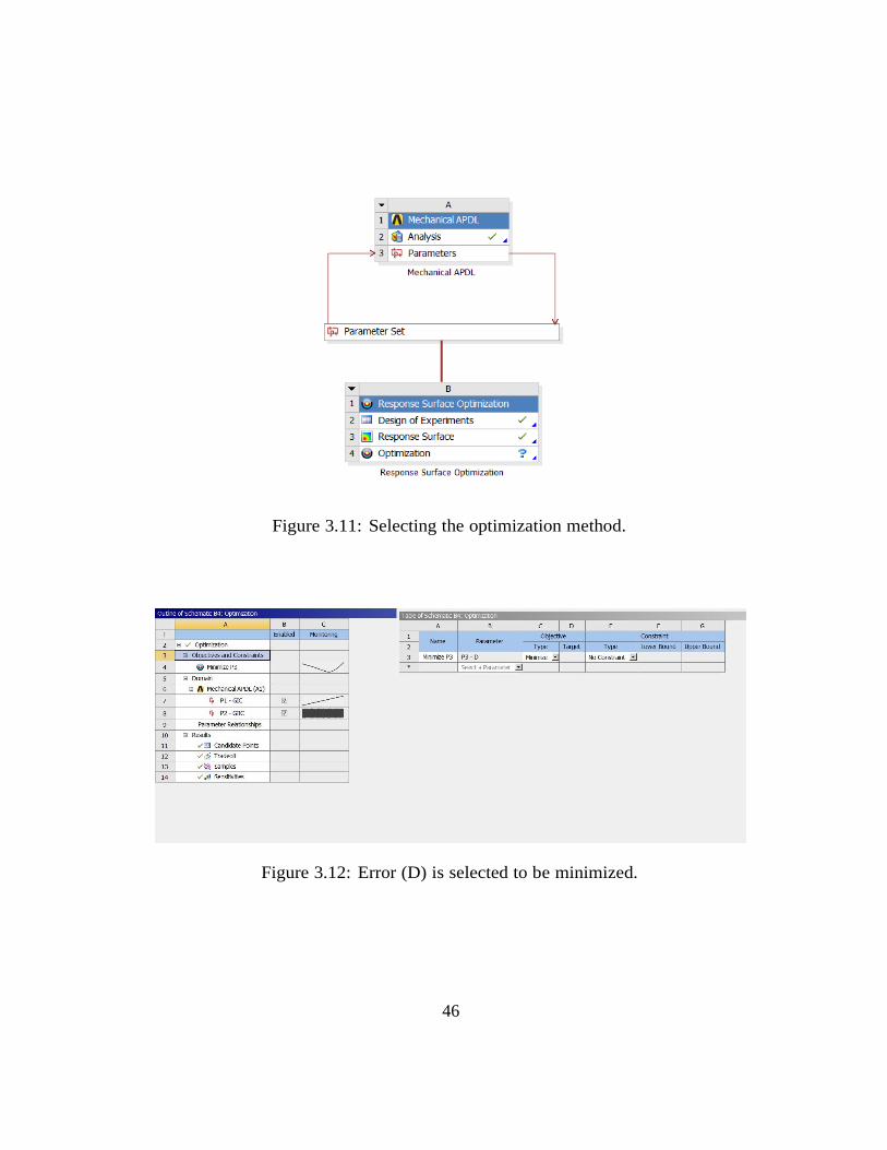
Figure 3.11: Selecting the optimization method.
Figure 3.12: Error (D) is selected to be minimized.
47
3.4 Comparison with experiments In this section, predicted laminate modulus Ex(Ex) with parameters listed in Table 3.7 are
compared with experimental data for all the laminates. The error for each laminate is
reported in Table 3.6.
Figure 3.13: ANSYS DDM and experimental data normalized modulus vs. crack density
(cr/mm) curves for laminate #1.
48
Figure 3.14: Normalized modulus vs. applied strain for laminate #2.
Figure 3.15: Normalized modulus vs. applied strain for laminate #3.
49
Figure 3.16: Normalized modulus vs. applied strain for laminate #4.
Figure 3.17: Normalized modulus vs. applied strain for laminate #5.
50
Figure 3.18: ANSYS DDM and experimental data crack density (cr/mm) vs. applied strain
curves for laminate #5.
51
Figure 3.19: ANSYS DDM and experimental data normalized modulus vs. crack density
(cr/mm) curves for laminate #5.
52
Figure 3.20: Normalized modulus vs. applied strain for laminate #6.
Figure 3.21: ANSYS DDM and experimental data crack density (cr/mm) vs. applied strain
curves for laminate #6.
53
Figure 3.22: ANSYS DDM and experimental data normalized modulus vs. crack density
(cr/mm) curves for laminate #6.
Figure 3.23: Normalized modulus vs. applied strain for laminate #7.
54
Figure 3.24: ANSYS DDM and experimental data crack density (cr/mm) vs. applied strain
curves for laminate #7.
55
Figure 3.25: ANSYS DDM and experimental data normalized modulus vs. crack density
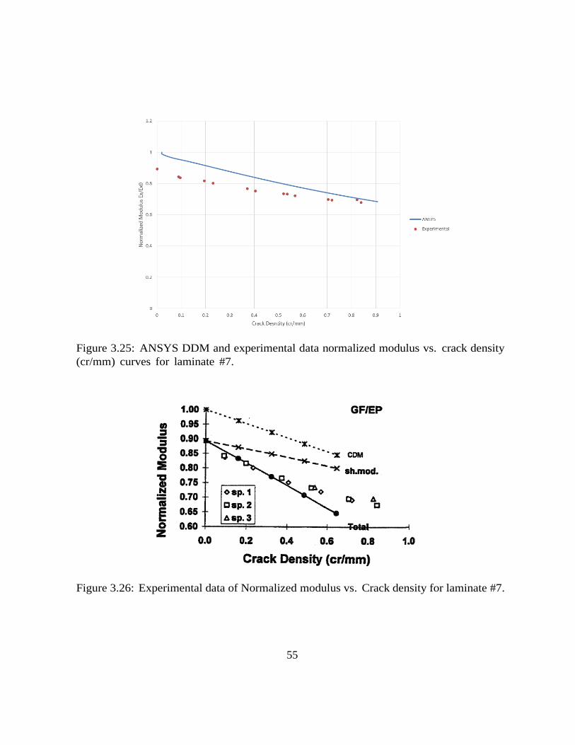
(cr/mm) curves for laminate #7.
Figure 3.26: Experimental data of Normalized modulus vs. Crack density for laminate #7.
56
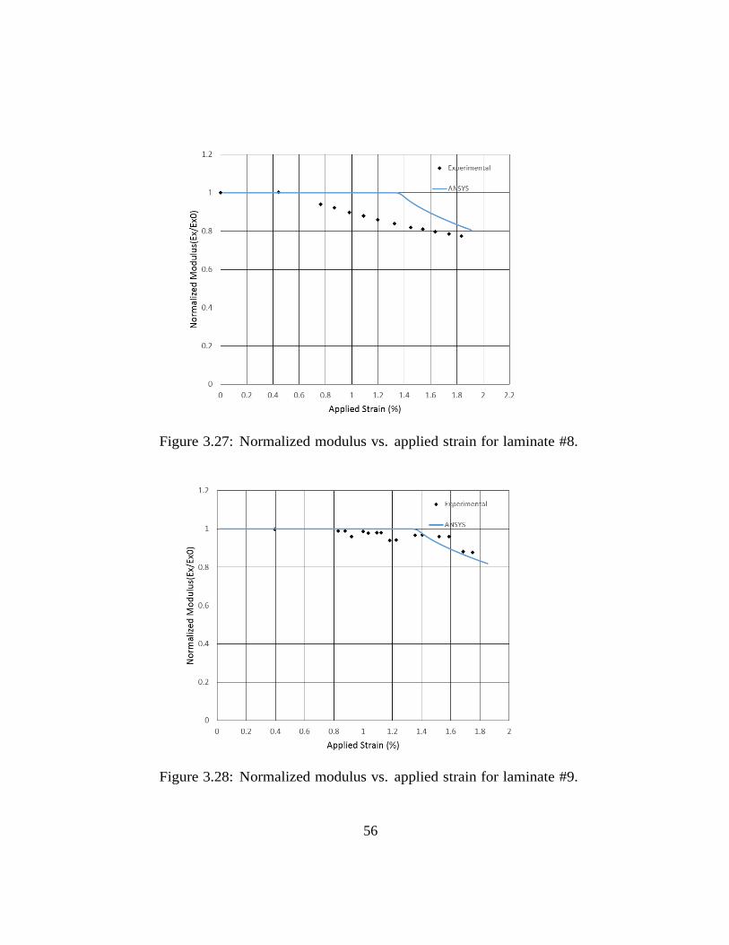
Figure 3.27: Normalized modulus vs. applied strain for laminate #8.
Figure 3.28: Normalized modulus vs. applied strain for laminate #9.
57
As shown in Figures of this section (Fig.3.13–Fig.3.28) the adjusted values work well
for almost all types of laminate except Laminates #6 and #8.
The only way to fi laminate #6’s results is to decrease the GIc to 0.23 instead of current
adjusted value which is 0.438, but it is not a good idea because it changes the results for
laminate #1 to #5, and since we adjusted the GIc by laminate #1 it is reasonable to have
the best fi for laminate #1.
About Laminate #8, the discrepancies can be eliminated by decreasing the GIIc, but
ANSYS crashes for GIIc less than 0.8, so it was not possible to check the values less than
0.8 by ANSYS.
3.5 Mesh sensitivity Mesh sensitivity refers to how much the solution changes with mesh density, number of
elements, or number of nodes used to discretize the problem under study. There are two
sources of mesh sensitivity. The most obvious is type I sensitivity, where the quality of
the solution, particularly stress and strain gradients, depends on mesh density; the fi
the mesh, the better the accuracy of the solution. Assuming that the mesh is refined
enough to capture stress/strain gradients satisfactorily, type II sensitivity may come from
the constitutive model used. When the material response is non-linear, the constitutive
model calculates the stress for a given strain and updates one or more state variables to
keep track of the history of the material state. Ideally, the response of the constitutive
model should be independent of the mesh. To isolate the two sources of mesh dependency,
it is customary to test the software with examples for which the strain fi is uniform in
the domain regardless of mesh density. The physical tensile test in this study experiences
uniform strain everywhere in the rectangular domain representing the gage section of the
specimen. Under these conditions, the reaction force calculated by FEA for a given applied
strain should be independent of the mesh. There is no type I mesh sensitivity in the
calculation of displacement and strain because the strain is uniform in the entire domain.
But the reaction force depends on the accuracy of the constitutive model. It can be seen
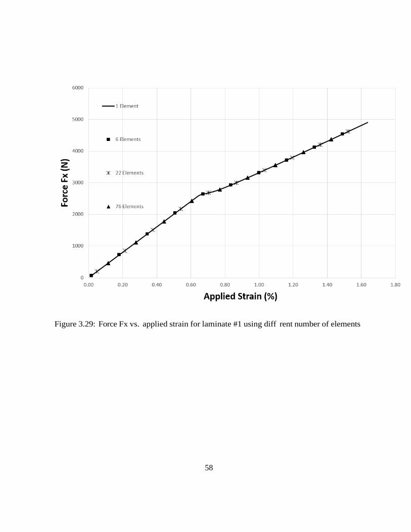
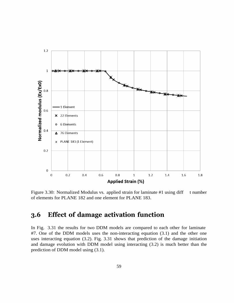
in Fig. 3.30 that DDM is mesh insensitive.
58
Figure 3.29: Force Fx vs. applied strain for laminate #1 using diff rent number of elements
59
Figure 3.30: Normalized Modulus vs. applied strain for laminate #1 using diff t number
of elements for PLANE 182 and one element for PLANE 183.
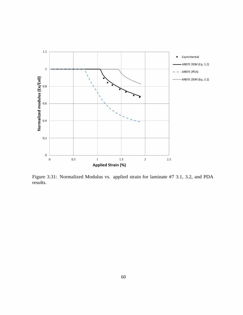
3.6 Effect of damage activation function In Fig. 3.31 the results for two DDM models are compared to each other for laminate
#7. One of the DDM models uses the non-interacting equation (3.1) and the other one
uses interacting equation (3.2). Fig. 3.31 shows that prediction of the damage initiation
and damage evolution with DDM model using interacting (3.2) is much better than the
prediction of DDM model using (3.1).
60
Figure 3.31: Normalized Modulus vs. applied strain for laminate #7 3.1, 3.2, and PDA
results.
61
Chapter 4 Conclusions and Future Work
4.1 Conclusions This study shows that adjusted transverse and shear strengths (in situ values) predict
the damage initiation and evolution for the PDA by comparing the implemented data
from ANSYS with available experimental data for nine diff t laminates. Also, the
determination of material parameters for DDM give the best prediction damage behavior
for E-Glass Epoxy laminated composite. In other words, ANSYS users can use the adjusted
values in this thesis to predict damage behavior of any laminated composite they need and
get a good prediction for Normalized Modulus Vs. Applied strain with PDA or DDM
model (Apendix A.1 or A.2 ). Also, the user can predict the Crack Density Vs. Applied
Strain and Normalized Modulus Vs. Crack Density plots with DDM model and adjusted
material parameters in this thesis, as shown in (Fig. 3.25 and 3.24).
As shown in chapters 2 and 3, this study uses the same optimization method to adjust
the material parameters for both PDA and DDM models. This methodology can be used
for different optimization purposes, and is explained step by step in this thesis that give this
opportunity to the ANSYS users to use the strong ANSYS optimization tools instead of
writing optimization codes in MATLAB and linking MATLAB with ANSYS. Regarding the
mesh sensitivity, ANSYS PDA is dependent to the mesh type and element size, although
DDM model does not show any sensitivity to neither p- or h-refi ment. It shows that
DDM adjusted values work for all mesh type and element sizes, but for PDA the material
parameters can be diff t for small elements or diff t types of element that can be
considered as future work.
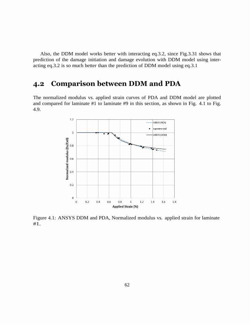
62
Also, the DDM model works better with interacting eq.3.2, since Fig.3.31 shows that
prediction of the damage initiation and damage evolution with DDM model using inter-
acting eq.3.2 is so much better than the prediction of DDM model using eq.3.1
4.2 Comparison between DDM and PDA The normalized modulus vs. applied strain curves of PDA and DDM model are plotted
and compared for laminate #1 to laminate #9 in this section, as shown in Fig. 4.1 to Fig.
4.9.
Figure 4.1: ANSYS DDM and PDA, Normalized modulus vs. applied strain for laminate
#1.
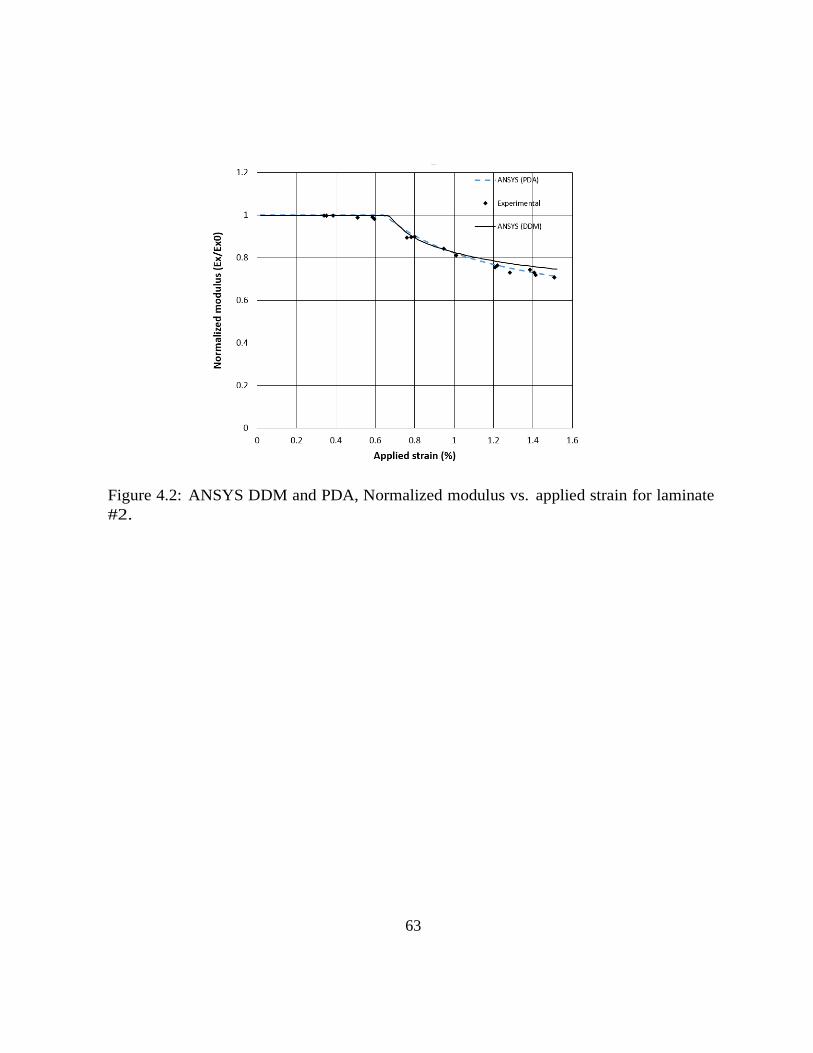
63
Figure 4.2: ANSYS DDM and PDA, Normalized modulus vs. applied strain for laminate
#2.
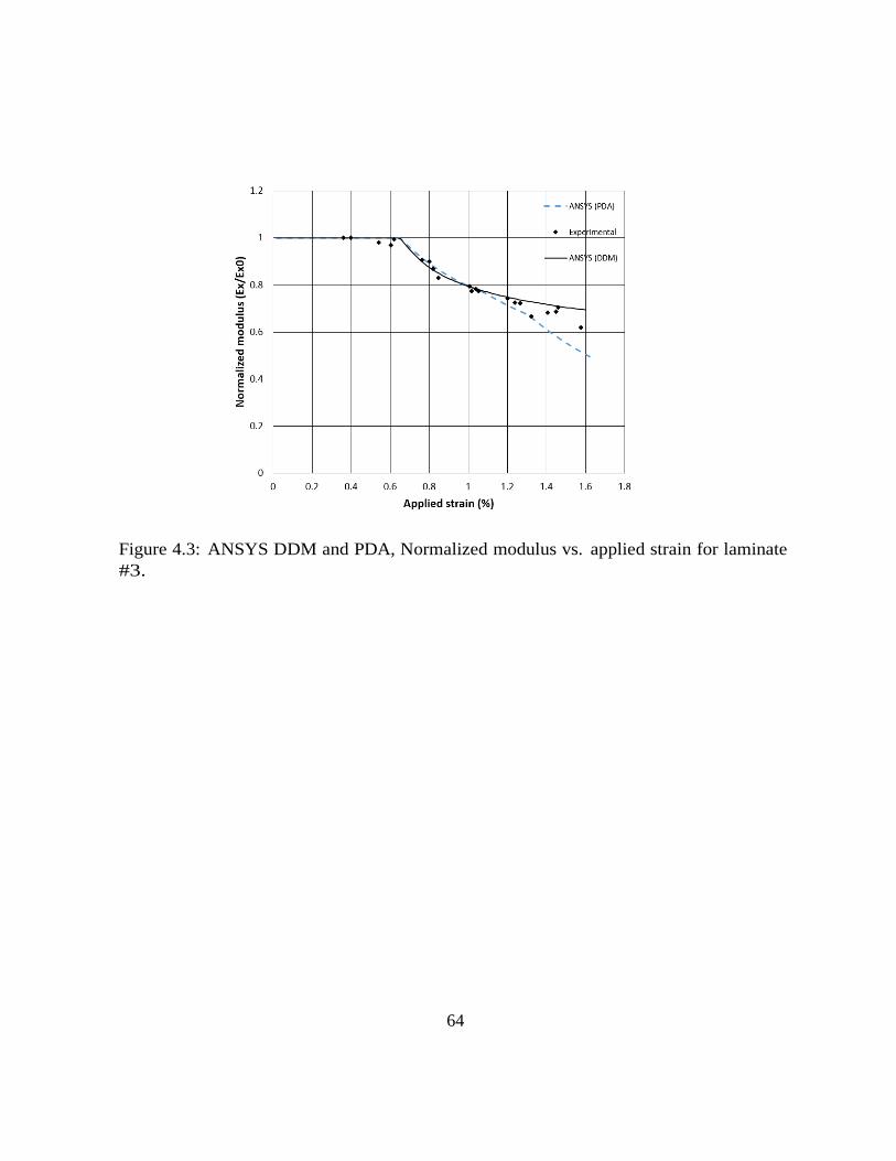
64
Figure 4.3: ANSYS DDM and PDA, Normalized modulus vs. applied strain for laminate
#3.
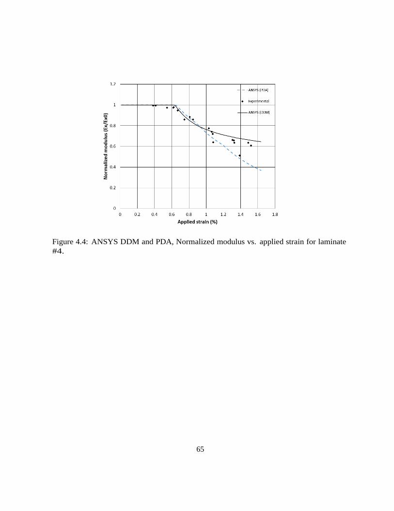
65
Figure 4.4: ANSYS DDM and PDA, Normalized modulus vs. applied strain for laminate
#4.
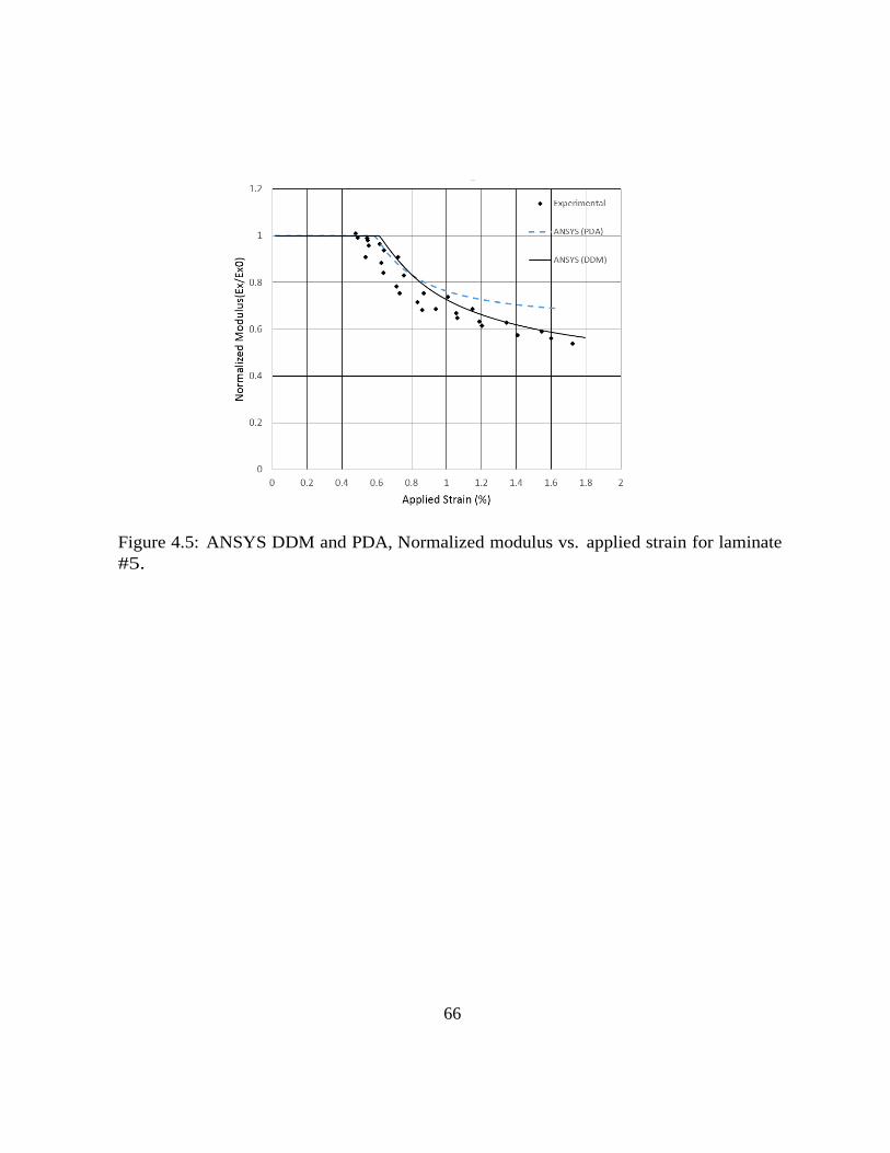
66
Figure 4.5: ANSYS DDM and PDA, Normalized modulus vs. applied strain for laminate
#5.
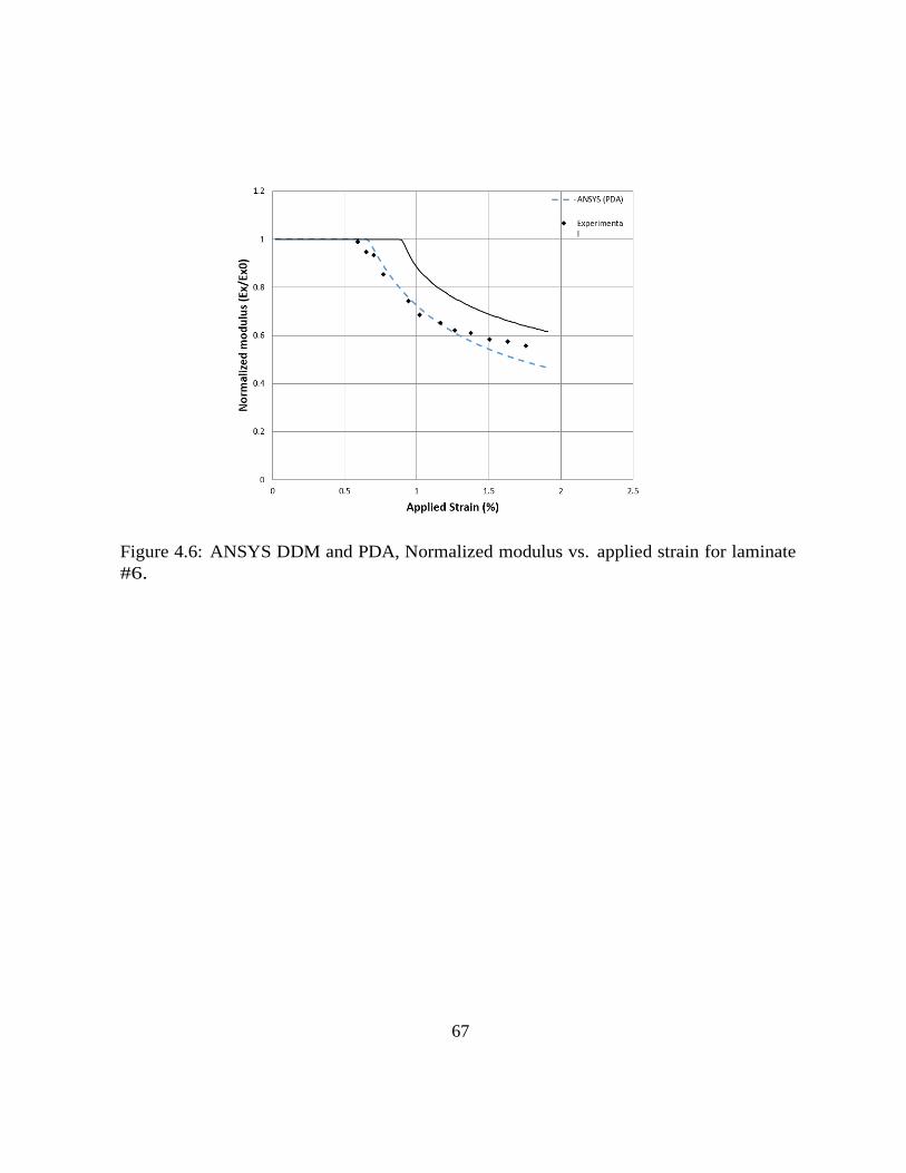
67
Figure 4.6: ANSYS DDM and PDA, Normalized modulus vs. applied strain for laminate
#6.
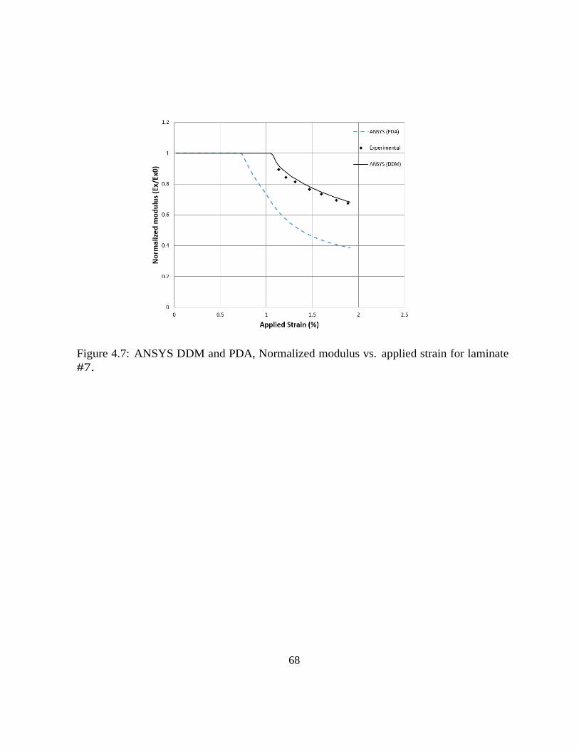
68
Figure 4.7: ANSYS DDM and PDA, Normalized modulus vs. applied strain for laminate
#7.
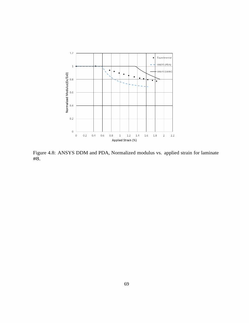
69
Figure 4.8: ANSYS DDM and PDA, Normalized modulus vs. applied strain for laminate
#8.
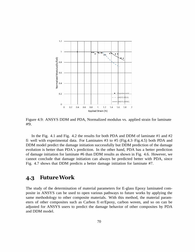
70
Figure 4.9: ANSYS DDM and PDA, Normalized modulus vs. applied strain for laminate
#9.
In the Fig. 4.1 and Fig. 4.2 the results for both PDA and DDM of laminate #1 and #2
fi well with experimental data. For Laminates #3 to #5 (Fig.4.3–Fig.4.5) both PDA and
DDM model predict the damage initiation successfully but DDM prediction of the damage
evolution is better than PDA’s prediction. In the other hand, PDA has a better prediction
of damage initiation for laminate #6 than DDM results as shown in Fig. 4.6. However, we
cannot conclude that damage initiation can always be predicted better with PDA, since
Fig. 4.7 shows that DDM predicts a better damage initiation for laminate #7.
4.3 Future Work The study of the determination of material parameters for E-glass Epoxy laminated com-
posite in ANSYS can be used to open various pathways to future works by applying the
same methodology to other composite materials. With this method, the material param-
eters of other composites such as Carbon fi er/Epoxy, carbon woven, and so on can be
adjusted for ANSYS users to predict the damage behavior of other composites by PDA
and DDM model.

71
The mesh sensitivity of both PDA and DDM are presented in this study. The mesh
sensitivity section shows that DDM Model is insensitive to the element type and size, but
PDA shows a high dependency to the element size. Adjusting material parameters for the
small elements can be considered as a future work.

72
APPENDICES
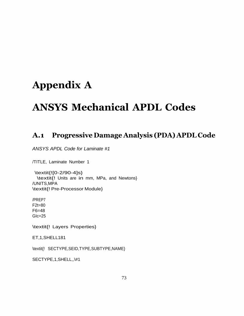
73
Appendix A ANSYS Mechanical APDL Codes
A.1 Progressive Damage Analysis (PDA) APDL Code ANSYS APDL Code for Laminate #1
/TITLE, Laminate Number 1
\textit{![0-2/90-4]s}
\textit{! Units are in mm, MPa, and Newtons}
/UNITS,MPA
\textit{! Pre-Processor Module}
/PREP7
F2t=80
F6=48
GIc=25
\textit{! Layers Properties}
ET,1,SHELL181
\textit{! SECTYPE,SEID,TYPE,SUBTYPE,NAME}
SECTYPE,1,SHELL,,\#1
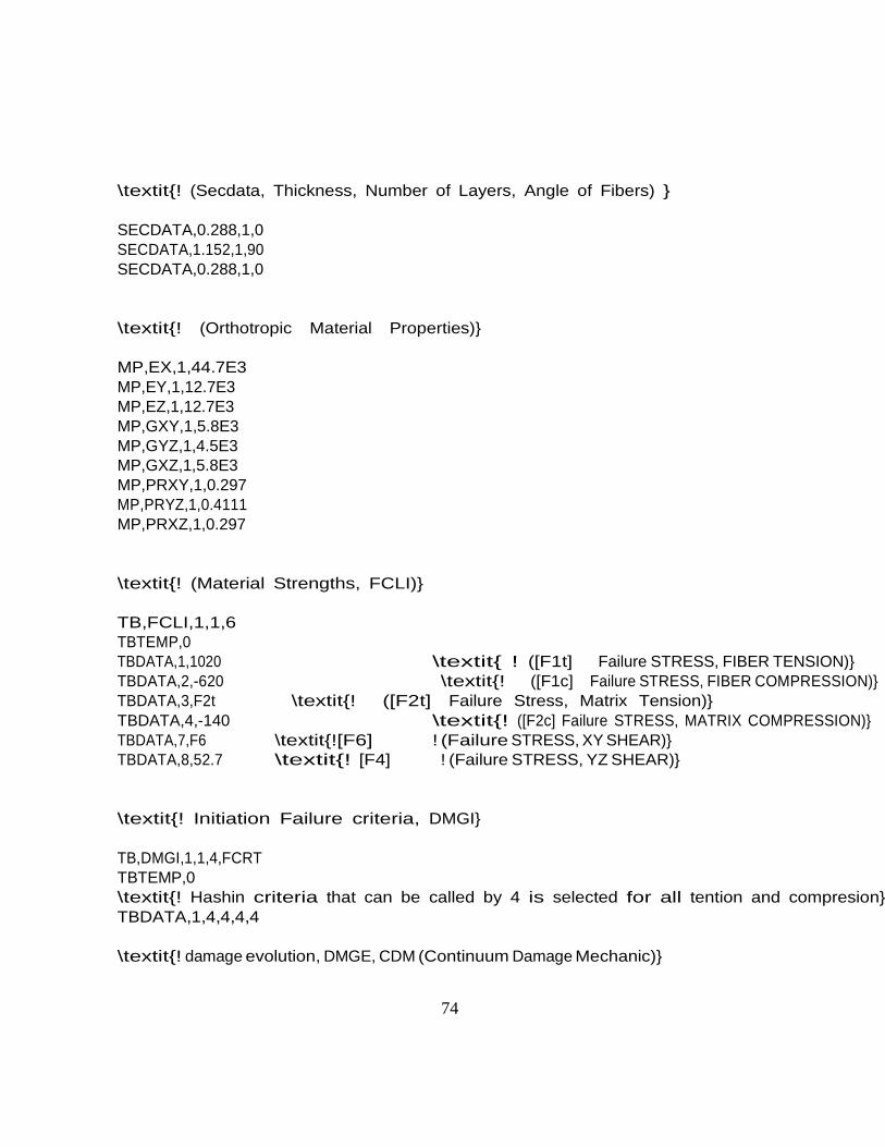
74
\textit{! (Secdata, Thickness, Number of Layers, Angle of Fibers) }
SECDATA,0.288,1,0
SECDATA,1.152,1,90
SECDATA,0.288,1,0
\textit{! (Orthotropic Material Properties)}
MP,EX,1,44.7E3
MP,EY,1,12.7E3
MP,EZ,1,12.7E3
MP,GXY,1,5.8E3
MP,GYZ,1,4.5E3
MP,GXZ,1,5.8E3
MP,PRXY,1,0.297
MP,PRYZ,1,0.4111
MP,PRXZ,1,0.297
\textit{! (Material Strengths, FCLI)}
TB,FCLI,1,1,6
TBTEMP,0
TBDATA,1,1020 \textit{ ! ([F1t] Failure STRESS, FIBER TENSION)}
TBDATA,2,-620 \textit{! ([F1c] Failure STRESS, FIBER COMPRESSION)}
TBDATA,3,F2t \textit{! ([F2t] Failure Stress, Matrix Tension)}
TBDATA,4,-140 \textit{! ([F2c] Failure STRESS, MATRIX COMPRESSION)}
TBDATA,7,F6 \textit{![F6] ! (Failure STRESS, XY SHEAR)}
TBDATA,8,52.7 \textit{! [F4] ! (Failure STRESS, YZ SHEAR)}
\textit{! Initiation Failure criteria, DMGI}
TB,DMGI,1,1,4,FCRT
TBTEMP,0
\textit{! Hashin criteria that can be called by 4 is selected for all tention and compresion}
TBDATA,1,4,4,4,4
\textit{! damage evolution, DMGE, CDM (Continuum Damage Mechanic)}
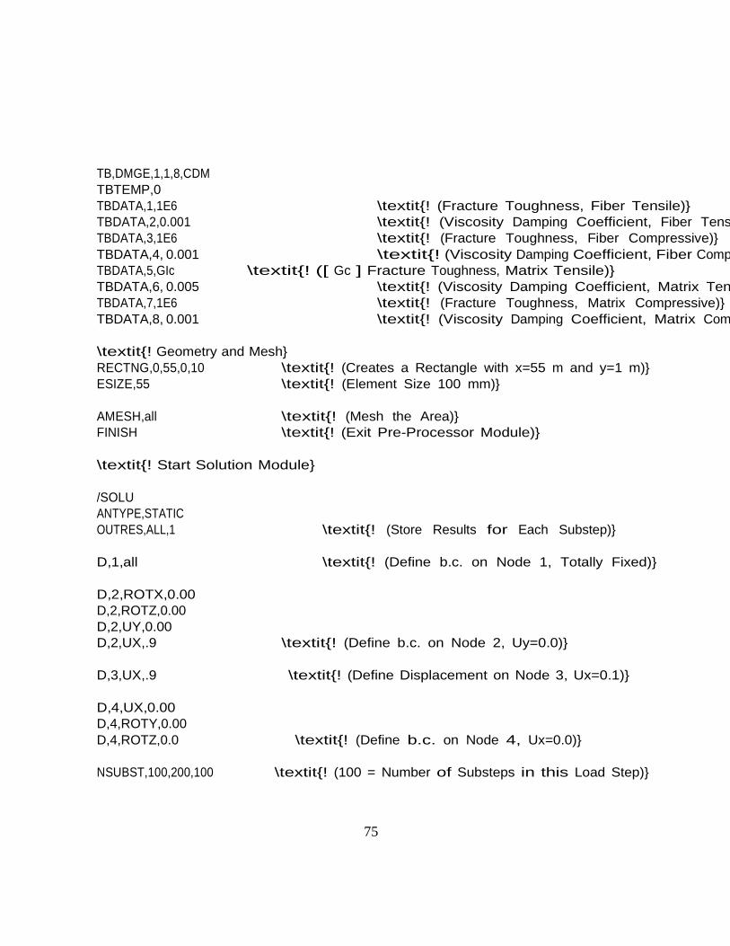
75
TB,DMGE,1,1,8,CDM
TBTEMP,0
TBDATA,1,1E6 \textit{! (Fracture Toughness, Fiber Tensile)}
TBDATA,2,0.001 \textit{! (Viscosity Damping Coefficient, Fiber Tens
TBDATA,3,1E6 \textit{! (Fracture Toughness, Fiber Compressive)}
TBDATA,4, 0.001 \textit{! (Viscosity Damping Coefficient, Fiber Comp
TBDATA,5,GIc \textit{! ([ Gc ] Fracture Toughness, Matrix Tensile)}
TBDATA,6, 0.005 \textit{! (Viscosity Damping Coefficient, Matrix Ten
TBDATA,7,1E6 \textit{! (Fracture Toughness, Matrix Compressive)}
TBDATA,8, 0.001 \textit{! (Viscosity Damping Coefficient, Matrix Com
\textit{! Geometry and Mesh}
RECTNG,0,55,0,10 \textit{! (Creates a Rectangle with x=55 m and y=1 m)}
ESIZE,55 \textit{! (Element Size 100 mm)}
AMESH,all \textit{! (Mesh the Area)}
FINISH \textit{! (Exit Pre-Processor Module)}
\textit{! Start Solution Module}
/SOLU
ANTYPE,STATIC
OUTRES,ALL,1 \textit{! (Store Results for Each Substep)}
D,1,all \textit{! (Define b.c. on Node 1, Totally Fixed)}
D,2,ROTX,0.00
D,2,ROTZ,0.00
D,2,UY,0.00
D,2,UX,.9 \textit{! (Define b.c. on Node 2, Uy=0.0)}
D,3,UX,.9 \textit{! (Define Displacement on Node 3, Ux=0.1)}
D,4,UX,0.00
D,4,ROTY,0.00
D,4,ROTZ,0.0 \textit{! (Define b.c. on Node 4, Ux=0.0)}
NSUBST,100,200,100 \textit{! (100 = Number of Substeps in this Load Step)}
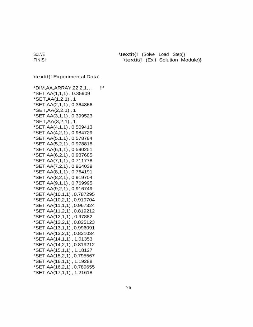
76
SOLVE \textit{! (Solve Load Step)}
FINISH \textit{! (Exit Solution Module)}
\textit{! Experimental Data}
*DIM,AA,ARRAY,22,2,1, , , !*
*SET,AA(1,1,1) , 0.35909
*SET,AA(1,2,1) , 1
*SET,AA(2,1,1) , 0.364866
*SET,AA(2,2,1) , 1
*SET,AA(3,1,1) , 0.399523
*SET,AA(3,2,1) , 1
*SET,AA(4,1,1) , 0.509413
*SET,AA(4,2,1) , 0.984729
*SET,AA(5,1,1) , 0.578784
*SET,AA(5,2,1) , 0.978818
*SET,AA(6,1,1) , 0.590251
*SET,AA(6,2,1) , 0.987685
*SET,AA(7,1,1) , 0.711778
*SET,AA(7,2,1) , 0.964039
*SET,AA(8,1,1) , 0.764191
*SET,AA(8,2,1) , 0.919704
*SET,AA(9,1,1) , 0.769995
*SET,AA(9,2,1) , 0.916749
*SET,AA(10,1,1) , 0.787295
*SET,AA(10,2,1) , 0.919704
*SET,AA(11,1,1) , 0.967324
*SET,AA(11,2,1) , 0.819212
*SET,AA(12,1,1) , 0.97882
*SET,AA(12,2,1) , 0.825123
*SET,AA(13,1,1) , 0.996091
*SET,AA(13,2,1) , 0.831034
*SET,AA(14,1,1) , 1.01353
*SET,AA(14,2,1) , 0.819212
*SET,AA(15,1,1) , 1.18127
*SET,AA(15,2,1) , 0.795567
*SET,AA(16,1,1) , 1.19288
*SET,AA(16,2,1) , 0.789655
*SET,AA(17,1,1) , 1.21618
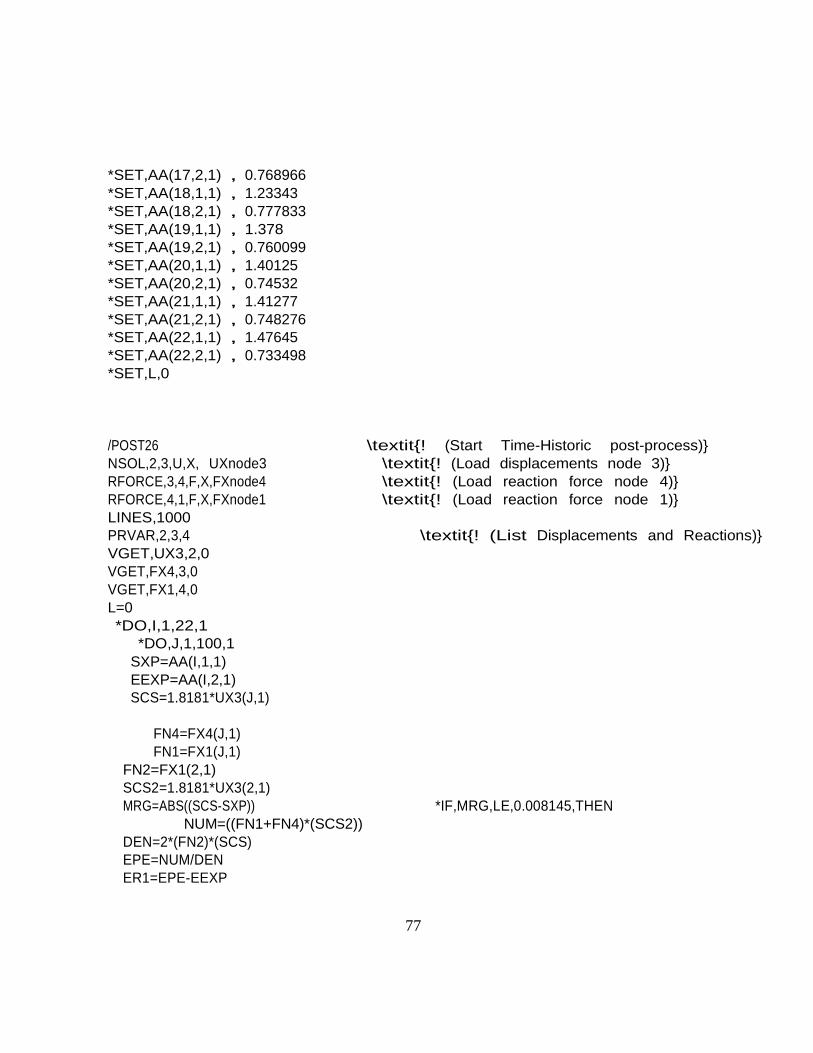
77
*SET,AA(17,2,1) , 0.768966
*SET,AA(18,1,1) , 1.23343
*SET,AA(18,2,1) , 0.777833
*SET,AA(19,1,1) , 1.378
*SET,AA(19,2,1) , 0.760099
*SET,AA(20,1,1) , 1.40125
*SET,AA(20,2,1) , 0.74532
*SET,AA(21,1,1) , 1.41277
*SET,AA(21,2,1) , 0.748276
*SET,AA(22,1,1) , 1.47645
*SET,AA(22,2,1) , 0.733498
*SET,L,0
/POST26 \textit{! (Start Time-Historic post-process)}
NSOL,2,3,U,X, UXnode3 \textit{! (Load displacements node 3)}
RFORCE,3,4,F,X,FXnode4 \textit{! (Load reaction force node 4)}
RFORCE,4,1,F,X,FXnode1 \textit{! (Load reaction force node 1)}
LINES,1000
PRVAR,2,3,4 \textit{! (List Displacements and Reactions)}
VGET,UX3,2,0
VGET,FX4,3,0
VGET,FX1,4,0
L=0
*DO,I,1,22,1
*DO,J,1,100,1
SXP=AA(I,1,1)
EEXP=AA(I,2,1)
SCS=1.8181*UX3(J,1)
FN4=FX4(J,1)
FN1=FX1(J,1)
FN2=FX1(2,1)
SCS2=1.8181*UX3(2,1)
MRG=ABS((SCS-SXP)) *IF,MRG,LE,0.008145,THEN
NUM=((FN1+FN4)*(SCS2))
DEN=2*(FN2)*(SCS)
EPE=NUM/DEN
ER1=EPE-EEXP
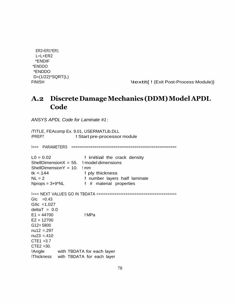
78
ER2=ER1*ER1
L=L+ER2
*ENDIF
*ENDDO
*ENDDO
D=(1/22)*SQRT(L)
FINISH \textit{ ! (Exit Post-Process Module)}
A.2 Discrete Damage Mechanics (DDM) Model APDL
Code
ANSYS APDL Code for Laminate #1 :
/TITLE, FEAcomp Ex. 9.01, USERMATLib.DLL
/PREP7 ! Start pre-processor module
!=== PARAMETERS ==================================================
L0 = 0.02 ! initial the crack density
ShellDimensionX = 55. ! model dimensions
ShellDimensionY = 10. ! mm
tk =.144 ! ply thickness
NL = 2 ! number layers half laminate
Nprops = 3+9*NL ! # material properties
!=== NEXT VALUES GO IN TBDATA ====================================
GIc =0.43
GIIc =1.027
deltaT = 0.0
E1 = 44700 ! MPa
E2 = 12700
G12= 5800
nu12 =.297
nu23 =.410
CTE1 =3.7
CTE2 =30.
!Angle with TBDATA for each layer
!Thickness with TBDATA for each layer
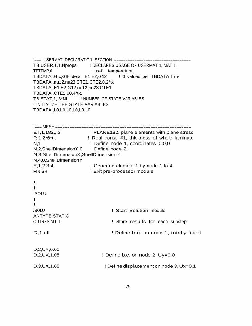
79
!=== USERMAT DECLARATION SECTION ==================================
TB,USER,1,1,Nprops, ! DECLARES USAGE OF USERMAT 1, MAT 1,
TBTEMP,0 ! ref. temperature
TBDATA,,GIc,GIIc,detaT,E1,E2,G12 ! 6 values per TBDATA line
TBDATA,,nu12,nu23,CTE1,CTE2,0,2*tk
TBDATA,,E1,E2,G12,nu12,nu23,CTE1
TBDATA,,CTE2,90,4*tk,
TB,STAT,1,,3*NL ! NUMBER OF STATE VARIABLES
! INITIALIZE THE STATE VARIABLES
TBDATA,,L0,L0,L0,L0,L0,L0
!=== MESH =========================================================
ET,1,182,,,3 ! PLANE182, plane elements with plane stress
R,1,2*6*tk ! Real const. #1, thickness of whole laminate
N,1 ! Define node 1, coordinates=0,0,0
N,2,ShellDimensionX,0 ! Define node 2,
N,3,ShellDimensionX,ShellDimensionY
N,4,0,ShellDimensionY
E,1,2,3,4 ! Generate element 1 by node 1 to 4
FINISH ! Exit pre-processor module
!
!
!SOLU
!
!
/SOLU ! Start Solution module
ANTYPE,STATIC
OUTRES,ALL,1 ! Store results for each substep
D,1,all ! Define b.c. on node 1, totally fixed
D,2,UY,0.00
D,2,UX,1.05 ! Define b.c. on node 2, Uy=0.0
D,3,UX,1.05 ! Define displacement on node 3, Ux=0.1
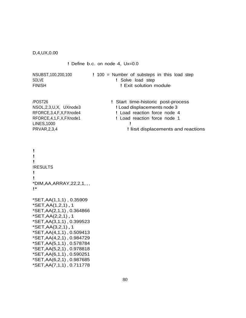
80
D,4,UX,0.00
! Define b.c. on node 4, Ux=0.0
NSUBST,100,200,100 ! 100 = Number of substeps in this load step
SOLVE ! Solve load step
FINISH ! Exit solution module
/POST26 ! Start time-historic post-process
NSOL,2,3,U,X, UXnode3 ! Load displacements node 3
RFORCE,3,4,F,X,FXnode4 ! Load reaction force node 4
RFORCE,4,1,F,X,FXnode1 ! Load reaction force node 1
LINES,1000 !
PRVAR,2,3,4 ! list displacements and reactions
!
!
!
!RESULTS
!
!
*DIM,AA,ARRAY,22,2,1, , ,
!*
*SET,AA(1,1,1) , 0.35909
*SET,AA(1,2,1) , 1
*SET,AA(2,1,1) , 0.364866
*SET,AA(2,2,1) , 1
*SET,AA(3,1,1) , 0.399523
*SET,AA(3,2,1) , 1
*SET,AA(4,1,1) , 0.509413
*SET,AA(4,2,1) , 0.984729
*SET,AA(5,1,1) , 0.578784
*SET,AA(5,2,1) , 0.978818
*SET,AA(6,1,1) , 0.590251
*SET,AA(6,2,1) , 0.987685
*SET,AA(7,1,1) , 0.711778
81
*SET,AA(7,2,1) , 0.964039
*SET,AA(8,1,1) , 0.764191
*SET,AA(8,2,1) , 0.919704
*SET,AA(9,1,1) , 0.769995
*SET,AA(9,2,1) , 0.916749
*SET,AA(10,1,1) , 0.787295
*SET,AA(10,2,1) , 0.919704
*SET,AA(11,1,1) , 0.967324
*SET,AA(11,2,1) , 0.819212
*SET,AA(12,1,1) , 0.97882
*SET,AA(12,2,1) , 0.825123
*SET,AA(13,1,1) , 0.996091
*SET,AA(13,2,1) , 0.831034
*SET,AA(14,1,1) , 1.01353
*SET,AA(14,2,1) , 0.819212
*SET,AA(15,1,1) , 1.18127
*SET,AA(15,2,1) , 0.795567
*SET,AA(16,1,1) , 1.19288
*SET,AA(16,2,1) , 0.789655
*SET,AA(17,1,1) , 1.21618
*SET,AA(17,2,1) , 0.768966
*SET,AA(18,1,1) , 1.23343
*SET,AA(18,2,1) , 0.777833
*SET,AA(19,1,1) , 1.378
*SET,AA(19,2,1) , 0.760099
*SET,AA(20,1,1) , 1.40125
*SET,AA(20,2,1) , 0.74532
*SET,AA(21,1,1) , 1.41277
*SET,AA(21,2,1) , 0.748276
*SET,AA(22,1,1) , 1.47645
*SET,AA(22,2,1) , 0.733498
*SET,L,0
VGET,UX3,2,0
VGET,FX4,3,0
VGET,FX1,4,0
L=0
*DO,I,1,22,1
82
*DO,J,1,100,1
SXP=AA(I,1,1)
EEXP=AA(I,2,1)
SCS=1.8181*UX3(J,1)
FN4=FX4(J,1)
FN1=FX1(J,1)
FN2=FX1(2,1)
SCS2=1.8181*UX3(2,1)
MRG=ABS((SCS-SXP)) *IF,MRG,LE,0.009545,THEN
NUM=((FN1+FN4)*(SCS2))
DEN=2*(FN2)*(SCS)
EPE=NUM/DEN
ER1=EPE-EEXP
ER2=ER1*ER1
L=L+ER2
*ENDIF
*ENDDO
*ENDDO
D=(1/22)*SQRT(L)
FINISH ! Exit post-process module
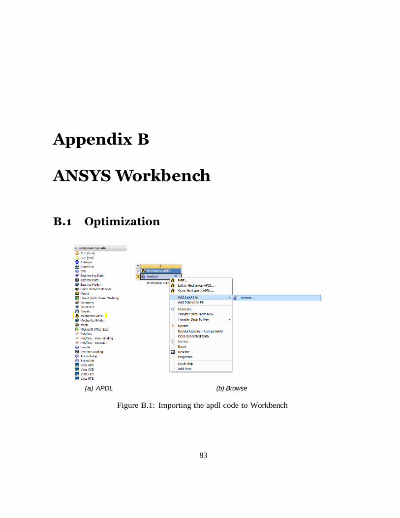
83
Appendix B
ANSYS Workbench
B.1 Optimization
(a) APDL (b) Browse
Figure B.1: Importing the apdl code to Workbench
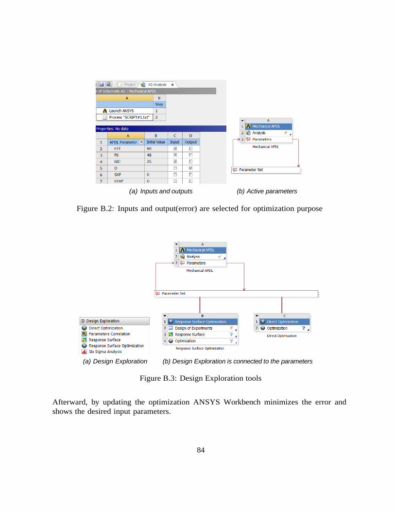
84
(a) Inputs and outputs (b) Active parameters
Figure B.2: Inputs and output(error) are selected for optimization purpose
(a) Design Exploration (b) Design Exploration is connected to the parameters
Figure B.3: Design Exploration tools
Afterward, by updating the optimization ANSYS Workbench minimizes the error and
shows the desired input parameters.
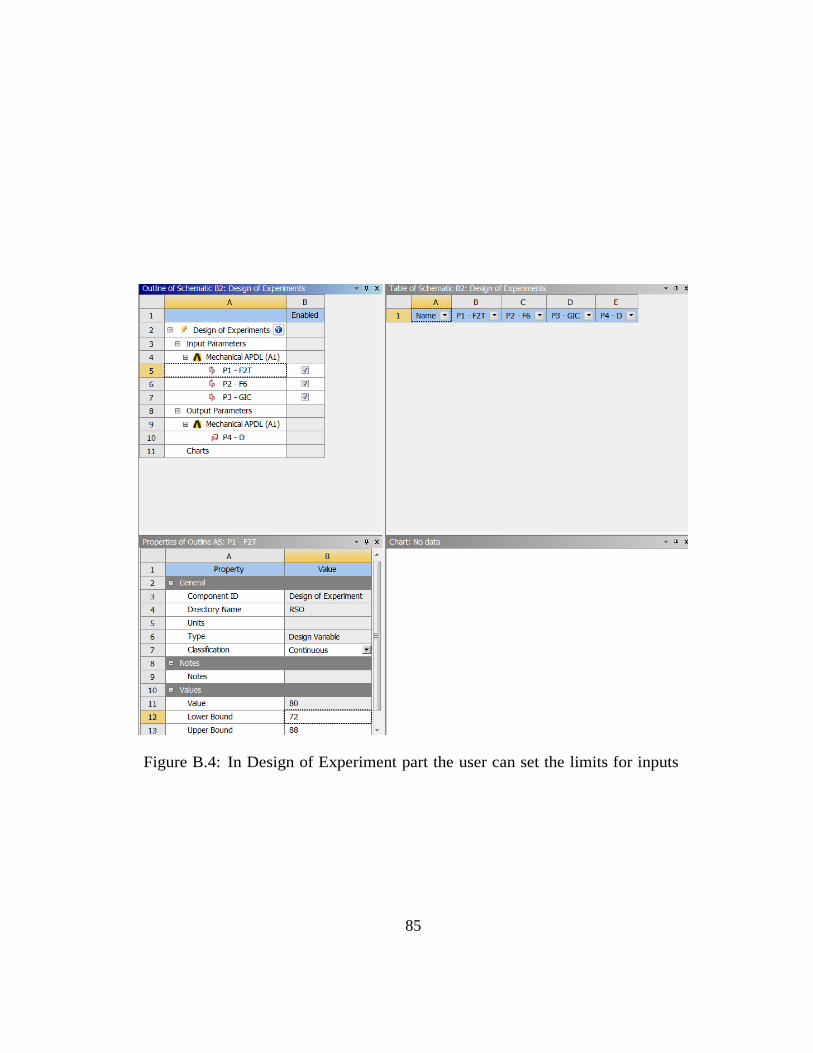
85
Figure B.4: In Design of Experiment part the user can set the limits for inputs
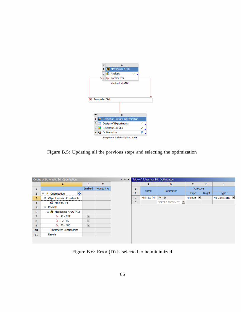
86
Figure B.5: Updating all the previous steps and selecting the optimization
Figure B.6: Error (D) is selected to be minimized
87
References
[1] Ansys mechanical apdl programmer’s manual, release 16.1. ANSYS Inc., 2 edition,
2016.
[2] G. Alfano and M.A. Crisfield. Finite element interface models for the delamination
analysis of laminated composites: Mechanical and computational issues. International
Journal for Numerical Methods in Engineering, 50(7):1701–1736, 2001. cited By 468.
[3] E. Barbero and D. Cortes. Constitutive model for elastic damage in fi er-reinforced
pmc laminae. International Journal of Damage Mechanics, 2001.
[4] E. Barbero and D. Cortes. A mechanistic model for transverse damage initiation,
evolution, and stiffness reduction in laminated composites. Composites Part B, 2010.
[5] E. J. Barbero. Finite Element Analysis of Composite Materials using ANSYS. 2
edition.
[6] E. J. Barbero. Introduction to Composite Materials Design. CRC Press, 2 edition,
2011.
[7] P.P. Camanho, C.G. Davila, S.T. Pinho, L. Iannucci, and P. Robinson. Prediction of
in situ strengths and matrix cracking in composites under transverse tension and in-
plane shear. Composites Part A: Applied Science and Manufacturing, 37(2):165–176,
2006. cited By 130.
[8] I.M. Daniel. Failure of composite materials. Strain, 2007.
[9] C.G. Davila, P.P. Camanho, and C.A. Rose. Failure criteria for frp laminates. Journal
of Composite Materials, 39(4):323–345, 2005.
88
[10] R. Roman E. J. Barbero, F. A. Cosso and T. L. Weadon. Determination of mate-
rial parameters for abaqus progressive damage analysis of e-glass epoxy lami- nates.
Composites Part B:Engineering, 2012.
[11] Z. Hashin. Failure criteria for unidirectional fi er composites. Journal of Applied
Mechanics, 1980.
[12] Z. Hashin and A. Rotem. Fatigue failure criterion for fi er reinforced materials. Jour-
nal of Composite Materials, 7:448–464, 1973.
[13] C.T. Herakovich. Mechanics of Fibrous Composite. John Wiley & Sons, Inc., New
York, 1998.
[14] Kaddour A.S. Hinton, M.J. and Soden. A comparison of the predictive capabilities of
current failure theories for composite laminates, judged against experimental evidence.
Composites Science and Technology, 2002.
[15] Soden P.D. Hinton, M.J. and Kaddour. Failure criteria in fi er-reinforced- polymer
composites. Elsevier, Oxford, 2004.
[16] Locatto S. Student G. Icardi, U. and Longo. Assessment of recent theories for pre-
dicting failure of composite laminates. Applied Mechanics Reviews, 2007.
[17] Carre‘ re N. Laurin, F. and J.F. Maire. A multiscale progressive failure approach
for composite laminates based on thermodynamical viscoelastic and damage mode.
Composites Part A: Applied Science and Manufacturing, 2007.
[18] Iannucci L. Pinho, S.T. and P. Robinson. Physically based failure models and crite-
ria for laminated fi forced composites with emphasis on fi kinking: Part i:
Development. Composites Part A: Applied Science and Manufacturing, 2006.
[19] Iannucci L. Pinho, S.T. and P. Robinson. Physically based failure models and criteria
for laminated fi composites with emphasis on fi kinking, part ii: Fe
implementation. Composites Part A: Applied Science and Manufacturing, 2006.
[20] A. Puck and H. Schu rmann. Failure analysis of frp laminates by means of physically
based phenomenological models. Composites Science and Technology, 1998.
[21] H. Wang A.K. Bledzki A. Korjakin R. Rikards, F.G. Buchholz and H.A. Richard. In-
vestigation of mixed mode i/ii interlaminar fracture toughness of laminated composites
by using a cts type specimen. Engineering Fracture Mechanics, 1998.
89
[22] C.T. Sun. Strength analysis of unidirectional composites and laminates. Comprehen-
sive Composite Materials, Elsevier Science, Ltd., Oxford, 2000.
[23] S.W. Tsai and E.M. Wu. A general theory of strength for anisotropic materials.
Journal of Composite Materials, 1971.
[24] J. Varna, R. Joffe, N.V. Akshantala, and R. Talreja. Damage in composite laminates
with off-axis plies. Composites Science and Technology, 59(14):2139–2147, 1999.
[25] J. Varna, R. Joffe, and R. Talreja. A synergistic damage-mechanics analysis of trans-
verse cracking [/904]s laminates. Composites Science and Technology, 61(5):657–665,
2001.