Embed Size (px)
Citation preview
Authoress: Ángela Santiago Dehesa UNIVERSIDAD DE CANTABRIA Escuela Técnica Superior de Ingenieros Industriales y de Telecomunicación Supervisor: Dr. W. Figiel, prof. PK POLITECHNIKA KRAKOWSKA Faculty of Chemical Engineering and Technology
CRACOW UNIVERSITY OF TECHNOLOGY Faculty of Chemical Engineering and
Technology
DETERMINATION OF EQUIVALENT
DIAMETERS FORIRREGULAR PARTICLES
February 2013
Ángela Santiago Dehesa February 2013
Page 1
INDEX
1. INTRODUCTION --------------------------------------------------------------------------- 4
1.1. JUSTIFICATION: OBJECTIVE OF STUDY ----------------------------------------------------------------------------- 5
2. DEFINITIONS ------------------------------------------------------------------------------ 7
2.1 EQUIVALENT DIAMETERS --------------------------------------------------------------------------------------------------- 7
2.1.1. Diameter of a sphere of equivalent volume (dV). -------------------------------------------------------- 7
2.1.2. Diameter of a sphere of equivalent area (dS). ------------------------------------------------------------ 7
2.1.3. Surface- volume diameter (dSV). ------------------------------------------------------------------------------ 7
2.1.4. Projected area diameter (da).---------------------------------------------------------------------------------- 8
2.1.5. Perimeter diameter (dC). ---------------------------------------------------------------------------------------- 9
2.1.6. Stokes diameter (dST). ------------------------------------------------------------------------------------------- 9
2.1.7. Martin diameter (dM) ------------------------------------------------------------------------------------------ 10
2.1.8. Feret diameter. (dF) -------------------------------------------------------------------------------------------- 10
2.1.9. Sieve diameter (dA). -------------------------------------------------------------------------------------------- 11
2.2. SPHERICITY. ------------------------------------------------------------------------------------------------------------- 12
2.3. SIZE MEASUREMENT-------------------------------------------------------------------------------------------------- 12
2.4. PARTICLE SHAPE CHARACTERIZATION -------------------------------------------------------------------------- 13
2.5. SETTLING VELOCITY OF AN ISOMETRIC PARTICLE ------------------------------------------------------------ 14
2.6. STOKES LAW ------------------------------------------------------------------------------------------------------------ 15
2.7. DENSITY OF SOLIDS --------------------------------------------------------------------------------------------------- 16
3. METHODOLOGY OF WORK ----------------------------------------------------------- 22
3.1. LABORATORY MATERIAL -------------------------------------------------------------------------------------------- 22
3.1.1. GLYCEROL --------------------------------------------------------------------------------------------------------- 22
Applications --------------------------------------------------------------------------------------------------------------------- 24
3.1.2. SOLIDS ------------------------------------------------------------------------------------------------------------- 25
3.1.3. INSTRUMENTS. -------------------------------------------------------------------------------------------------- 26
3.2. EXPERIMENTAL PROCEDURE --------------------------------------------------------------------------------------- 31
3.3. WORKING TOOLS ------------------------------------------------------------------------------------------------------ 32
4. RESULTS ---------------------------------------------------------------------------------- 34
4.1. PROCESS OF SAMPLE SELECTION --------------------------------------------------------------------------------- 34
4.2. CHARACTERISTICS OF GLYCEROL ---------------------------------------------------------------------------------- 35
Ángela Santiago Dehesa February 2013
Page 2
4.3. DATA PARTICLES ------------------------------------------------------------------------------------------------------- 37
4.3.1. Identification of particles ------------------------------------------------------------------------------------- 37
4.3.2. Microscope data ------------------------------------------------------------------------------------------------ 38
4.4. Solids density ----------------------------------------------------------------------------------------------------------- 39
4.5. Stokes law --------------------------------------------------------------------------------------------------------------- 41
4.6. Equivalent diameters ------------------------------------------------------------------------------------------------- 43
5. CONCLUSION ----------------------------------------------------------------------------- 46
6. BIBLIOGRAPHY ------------------------------------------------------------------------- 51

Ángela Santiago Dehesa February 2013
Page 3
INTRODUCTION
Ángela Santiago Dehesa February 2013
Page 4
1. INTRODUCTION
In the ideal world of the particle characterization, all the particles would be
homogeneous spheres. Moreover, they would have uniform properties such as
density, chemical composition, color, and opacity. Then, all the size
measurement methods would yield the same size for a particle, being its
diameter, and the same particle size distribution for a collection of particles,
regardless of the principle applied in the technique. It will be clear that such
particles would constitute the ideal standard reference material for particle size
measurement methods. It will also be clear that this world would be rather dull.
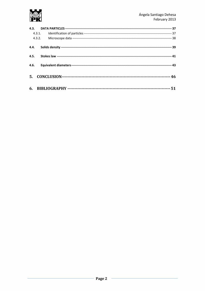
In the real world, most particles are not spherical, but have different shapes and
often rough surfaces. Materials of different chemical composition have different
properties and, even when the bulk composition is the same.
The size of spherical homogeneous particle is uniquely defined by its diameter.
For regular, compact particles such as cubes or regular tetrahedral, a single
dimension can be used to define the size. With some regular particles it may be
necessary to specify more than one dimension: for a cone the base diameter
and height are required whilst for a cuboid three dimensions are needed.
Derived diameters are determined by measuring a size-dependent property of
the particle and relating it to a single linear dimension. The most widely used of
these are the equivalent spherical diameters.
Ángela Santiago Dehesa February 2013
Page 5
1.1. JUSTIFICATION: OBJECTIVE OF STUDY
The aim of the study is to obtain a good method for finding the equivalent
diameter of irregular stones, taking account likewise what is the best way to
carry out the analysis.
Ángela Santiago Dehesa February 2013
Page 6
DEFINITIONS
Ángela Santiago Dehesa February 2013
Page 7
2. DEFINITIONS
2.1 EQUIVALENT DIAMETERS
The equivalent diameter is defined as "the diameter of a spherical particle that
would pass through a sieve with a certain opening x". This is done in order to
harmonize the irregularities of shapes in a form close to the sphere. Obviously it
is assumed as an inherent error in a granulate know that most of the particles
have different shapes.
Different types of equivalent diameters:
2.1.1. Diameter of a sphere of equivalent volume (dV).
Is the diameter of a sphere having the same volume (V) to the desired particle
characterization.
√
2.1.2. Diameter of a sphere of equivalent area (dS).
Is the diameter of a sphere having the same external surface (S) to the desired
particle characterization.
√
2.1.3. Surface- volume diameter (dSV).
Diameter of a sphere having the same eternal surface (S) to volume ratio (V) as
the particle
Ángela Santiago Dehesa February 2013
Page 8
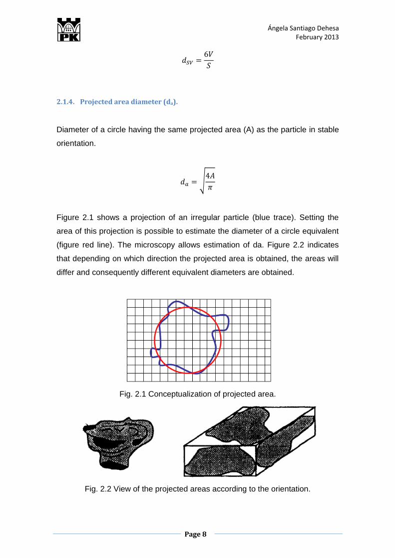
2.1.4. Projected area diameter (da).
Diameter of a circle having the same projected area (A) as the particle in stable
orientation.
√
Figure 2.1 shows a projection of an irregular particle (blue trace). Setting the
area of this projection is possible to estimate the diameter of a circle equivalent
(figure red line). The microscopy allows estimation of da. Figure 2.2 indicates
that depending on which direction the projected area is obtained, the areas will
differ and consequently different equivalent diameters are obtained.
Fig. 2.1 Conceptualization of projected area.
Fig. 2.2 View of the projected areas according to the orientation.
Ángela Santiago Dehesa February 2013
Page 9
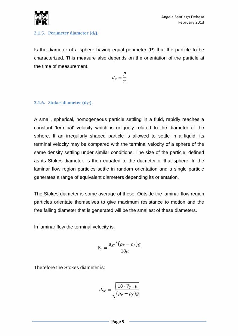
2.1.5. Perimeter diameter (dC).
Is the diameter of a sphere having equal perimeter (P) that the particle to be
characterized. This measure also depends on the orientation of the particle at
the time of measurement.
2.1.6. Stokes diameter (dST).
A small, spherical, homogeneous particle settling in a fluid, rapidly reaches a
constant ‘terminal’ velocity which is uniquely related to the diameter of the
sphere. If an irregularly shaped particle is allowed to settle in a liquid, its
terminal velocity may be compared with the terminal velocity of a sphere of the
same density settling under similar conditions. The size of the particle, defined
as its Stokes diameter, is then equated to the diameter of that sphere. In the
laminar flow region particles settle in random orientation and a single particle
generates a range of equivalent diameters depending its orientation.
The Stokes diameter is some average of these. Outside the laminar flow region
particles orientate themselves to give maximum resistance to motion and the
free falling diameter that is generated will be the smallest of these diameters.
In laminar flow the terminal velocity is:
( )
Therefore the Stokes diameter is:
√
( )
Ángela Santiago Dehesa February 2013
Page 10
Thus μ and ρf is the fluid viscosity and density, respectively. ΡP is the particle
density.
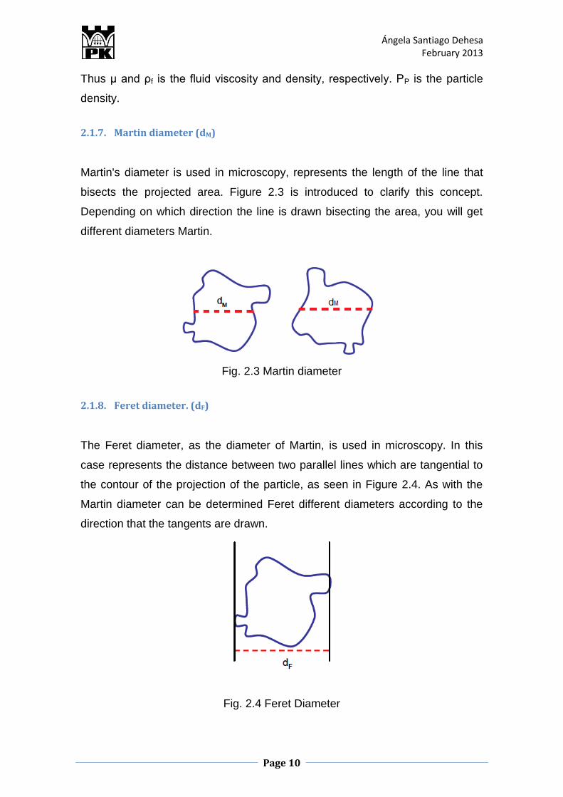
2.1.7. Martin diameter (dM)
Martin's diameter is used in microscopy, represents the length of the line that
bisects the projected area. Figure 2.3 is introduced to clarify this concept.
Depending on which direction the line is drawn bisecting the area, you will get
different diameters Martin.
Fig. 2.3 Martin diameter
2.1.8. Feret diameter. (dF)
The Feret diameter, as the diameter of Martin, is used in microscopy. In this
case represents the distance between two parallel lines which are tangential to
the contour of the projection of the particle, as seen in Figure 2.4. As with the
Martin diameter can be determined Feret different diameters according to the
direction that the tangents are drawn.
Fig. 2.4 Feret Diameter
Ángela Santiago Dehesa February 2013
Page 11
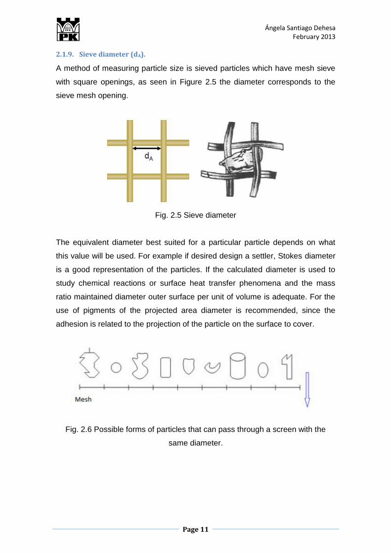
2.1.9. Sieve diameter (dA).
A method of measuring particle size is sieved particles which have mesh sieve
with square openings, as seen in Figure 2.5 the diameter corresponds to the
sieve mesh opening.
Fig. 2.5 Sieve diameter
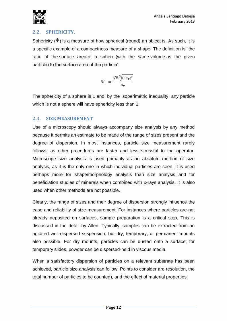
The equivalent diameter best suited for a particular particle depends on what
this value will be used. For example if desired design a settler, Stokes diameter
is a good representation of the particles. If the calculated diameter is used to
study chemical reactions or surface heat transfer phenomena and the mass
ratio maintained diameter outer surface per unit of volume is adequate. For the
use of pigments of the projected area diameter is recommended, since the
adhesion is related to the projection of the particle on the surface to cover.
Fig. 2.6 Possible forms of particles that can pass through a screen with the
same diameter.
Ángela Santiago Dehesa February 2013
Page 12
2.2. SPHERICITY.
Sphericity ( ) is a measure of how spherical (round) an object is. As such, it is
a specific example of a compactness measure of a shape. The definition is “the
ratio of the surface area of a sphere (with the same volume as the given
particle) to the surface area of the particle”.
√
√
The sphericity of a sphere is 1 and, by the isoperimetric inequality, any particle
which is not a sphere will have sphericity less than 1.
2.3. SIZE MEASUREMENT
Use of a microscopy should always accompany size analysis by any method
because it permits an estimate to be made of the range of sizes present and the
degree of dispersion. In most instances, particle size measurement rarely
follows, as other procedures are faster and less stressful to the operator.
Microscope size analysis is used primarily as an absolute method of size
analysis, as it is the only one in which individual particles are seen. It is used
perhaps more for shape/morphology analysis than size analysis and for
beneficiation studies of minerals when combined with x-rays analysis. It is also
used when other methods are not possible.
Clearly, the range of sizes and their degree of dispersion strongly influence the
ease and reliability of size measurement. For instances where particles are not
already deposited on surfaces, sample preparation is a critical step. This is
discussed in the detail by Allen. Typically, samples can be extracted from an
agitated well-dispersed suspension, but dry, temporary, or permanent mounts
also possible. For dry mounts, particles can be dusted onto a surface; for
temporary slides, powder can be dispersed-held in viscous media.
When a satisfactory dispersion of particles on a relevant substrate has been
achieved, particle size analysis can follow. Points to consider are resolution, the
total number of particles to be counted), and the effect of material properties.
Ángela Santiago Dehesa February 2013
Page 13
The microscope gives us data as aspect ratio, area, CE diameter, circularity,
convexity, elongation, length or width.
2.4. PARTICLE SHAPE CHARACTERIZATION
Particles have various shapes depending on their manufacturing method and
mechanical properties. Unlike a sphere or a rectangular parallelepiped, which
are objects with clear geometrical definitions, powder particles are very
complicated objects with no definite form. It is generally very difficult to describe
their shapes. They have therefore been conventionally described and classified
by the use of various terms.
On the other hand, along with recent rapid advances in computer and
information technologies, image processing technology has remarkably
progressed in both software and hardware, making it easy to obtain image
information and geometrical features of particles. Accordingly, various
quantitative methods for expressing particle shape have been proposed and
adopted.
The particle shape description or expression is classified by several criteria. In
the most primitive manner, the descriptions are classified into classified into
quantitative methods and qualitative ones.
In qualitative description, the shape is expressed by several terms such as
“spherical”, “granular”, “blocky”, “flaky”, “platy”, “prismodal”, “rodlike”, “acicular”,
“fibrous”, “irregular”, and so on. The verbal description is sometimes convenient
to express irregular shape and makes it easy to understand the shape visually.
But how are platy shape and a flaky shape distinguished? Under present
conditions, this distinction must depend on human visual judgments in many
cases. Therefore, quantitative descriptions of particle shape will be necessary.
Quantitative shape descriptors can be calculated from 2 or 3 dimensional
geometrical properties and can be calculated by comparing with physical
properties of the reference shape.
Ángela Santiago Dehesa February 2013
Page 14
The following are required for the shape descriptor:
Rotation invariance: values of the descriptor should be the same in any
orientation.
Scale invariance: values of the descriptor should be the same for
identical shapes of different size.
Reflection invariance.
Independence: if the elements of the descriptors are independent, some
can be discarded without the need to recalculate the others.
Uniqueness: one shape always should produce the same set of
descriptors, and one set of descriptors should describe only one shape.
Parsimony: it is desirable that the descriptors are thrifty in the number of
terms used to describe a shape.
2.5. SETTLING VELOCITY OF AN ISOMETRIC PARTICLE
The experimental device includes a mechanism of conditioning the
sedimentation of solid particles and a system of measurement based on a
space-time location. This method offers the advantage to not disturb the flow.
The sedimentation device consists of a glass column of 10.7 cm of radio and
1.20 m height, bearing in minds only 80cm of route.
The dimensions of the measurement column are selected by taking in to
account the practical requirements of the laboratory and the experimental
conditions but also having in mind the minimization of the influence of the wall
on the settling velocity.
The sedimentation test velocity is higher in infinite medium than the
sedimentation velocity in column. in an unlimited field, the fall of particle induces
the same speed direction in all points of the fluid and the drive effects is felt far
from the particle. On the other hand, in a limited field, the flow of the fluid is
constrained. The drive effect is induced near by the particle, generating a return
movement of the fluid, associated with viscous frictions at the wall.
Ángela Santiago Dehesa February 2013
Page 15
2.6. STOKES LAW
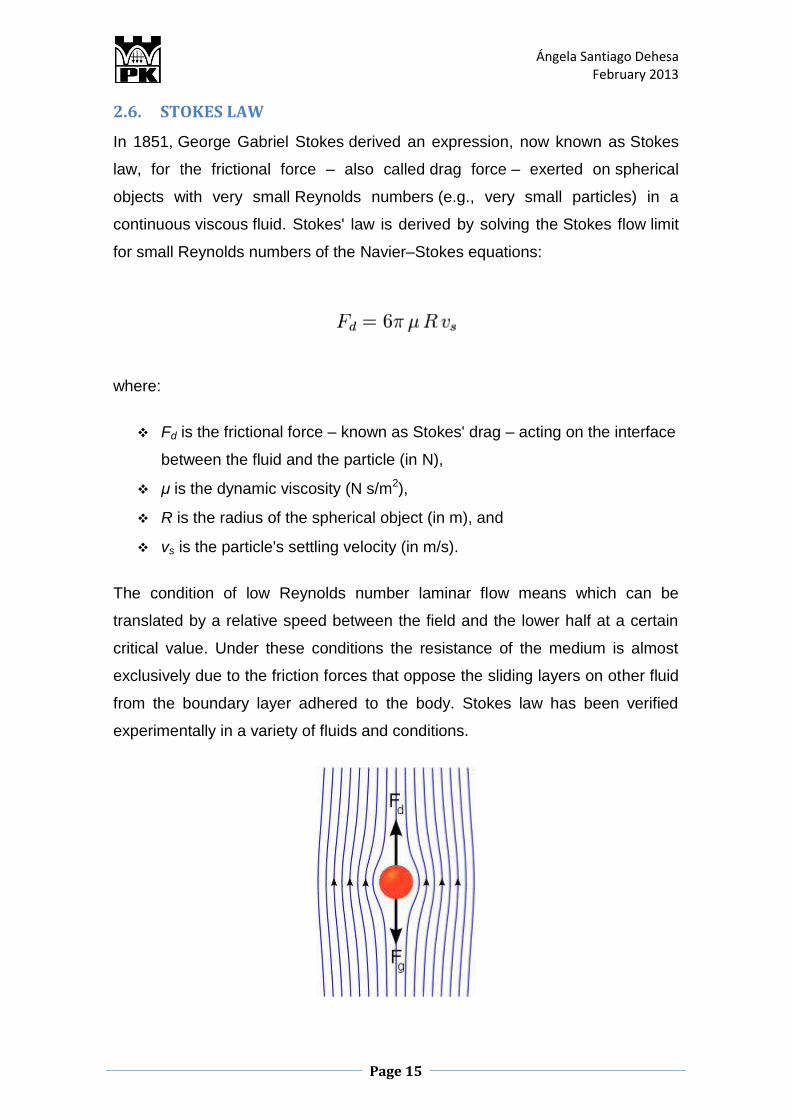
In 1851, George Gabriel Stokes derived an expression, now known as Stokes
law, for the frictional force – also called drag force – exerted on spherical
objects with very small Reynolds numbers (e.g., very small particles) in a
continuous viscous fluid. Stokes' law is derived by solving the Stokes flow limit
for small Reynolds numbers of the Navier–Stokes equations:
where:
Fd is the frictional force – known as Stokes' drag – acting on the interface
between the fluid and the particle (in N),
μ is the dynamic viscosity (N s/m2),
R is the radius of the spherical object (in m), and
vs is the particle's settling velocity (in m/s).
The condition of low Reynolds number laminar flow means which can be
translated by a relative speed between the field and the lower half at a certain
critical value. Under these conditions the resistance of the medium is almost
exclusively due to the friction forces that oppose the sliding layers on other fluid
from the boundary layer adhered to the body. Stokes law has been verified
experimentally in a variety of fluids and conditions.
Ángela Santiago Dehesa February 2013
Page 16
If the particles are falling vertically into a viscous fluid due to its own weight can
be calculated sedimentation velocity equaling or fall of frictional force with the
apparent weight of the particle in the fluid.
where:
vs is the particles' settling velocity (m/s) (vertically downwards if ρp > ρf,
upwards if ρp < ρf ),
g is the gravitational acceleration (m/s2),
ρp is the mass density of the particles (kg/m3), and
ρf is the mass density of the fluid (kg/m3).
Stokes' law makes the following assumptions for the behavior of a particle in a
fluid:
Laminar Flow
Spherical particles
Homogeneous (uniform in composition) material
Smooth surfaces
Particles do not interfere with each other.
2.7. DENSITY OF SOLIDS
An important feature of the solid particles (both small powders, such as large,
fruit) is its density. We should begin by distinguishing between the density per
unit density sometimes called "real", and the overall density or "apparent". The
first is the average mass per unit volume of the individual particles. Is
determined by weighing the particles in air and determining its volume by
displacement of a liquid, generally water. The ratio of weight (kg) divided by
volume (m3) is the actual density. If the particle size is small, employing a
gradient tube filled with two miscible liquids of different densities and allowed to
equilibrate for several days. Are introduced into the glass beads of known

Ángela Santiago Dehesa February 2013
Page 17
density are measured height which are, at constant temperature, and is a graph
representing the density function of the height. And calibrating the gradient, the
sample is introduced and its density is determined based on the height reached
in the tube by reference to the calibration graph.
The absolute density: is defined as the ratio of the mass per unit volume of a
body at a given temperature.
Where:
M: mass in Kg
V: Volume in m3
The absolute density is a function of temperature and pressure. The density of
some liquids in function of the temperature. The variation of the density of the
liquid is very small, except at very high pressures and for all practical
calculations can be neglected.
Relative density is defined as the ratio of the density of the substance with
respect to the pattern density, which leads to a relationship between the mass
of the test substance to the mass of the same volume of distilled water at
pressure atmosphere and 4 ° C. It is evident that the relative density is a
dimensionless quantity:
Substituting
Ángela Santiago Dehesa February 2013
Page 18
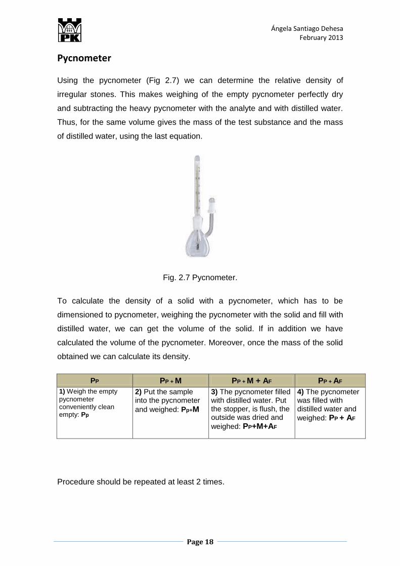
Pycnometer
Using the pycnometer (Fig 2.7) we can determine the relative density of
irregular stones. This makes weighing of the empty pycnometer perfectly dry
and subtracting the heavy pycnometer with the analyte and with distilled water.
Thus, for the same volume gives the mass of the test substance and the mass
of distilled water, using the last equation.
Fig. 2.7 Pycnometer.
To calculate the density of a solid with a pycnometer, which has to be
dimensioned to pycnometer, weighing the pycnometer with the solid and fill with
distilled water, we can get the volume of the solid. If in addition we have
calculated the volume of the pycnometer. Moreover, once the mass of the solid
obtained we can calculate its density.
PP PP + M PP + M + AF PP + AF
1) Weigh the empty pycnometer conveniently clean empty: Pp
2) Put the sample into the pycnometer
and weighed: Pp+M
3) The pycnometer filled with distilled water. Put the stopper, is flush, the outside was dried and
weighed: PP+M+AF
4) The pycnometer was filled with distilled water and
weighed: PP + AF
Procedure should be repeated at least 2 times.
Ángela Santiago Dehesa February 2013
Page 19
Calculations:
2) – 1) = Solid mass M
4) – 1) = Water mass A
3) – 2) = not dislodged water AF
A – AF= Dislodged water → Solid volume
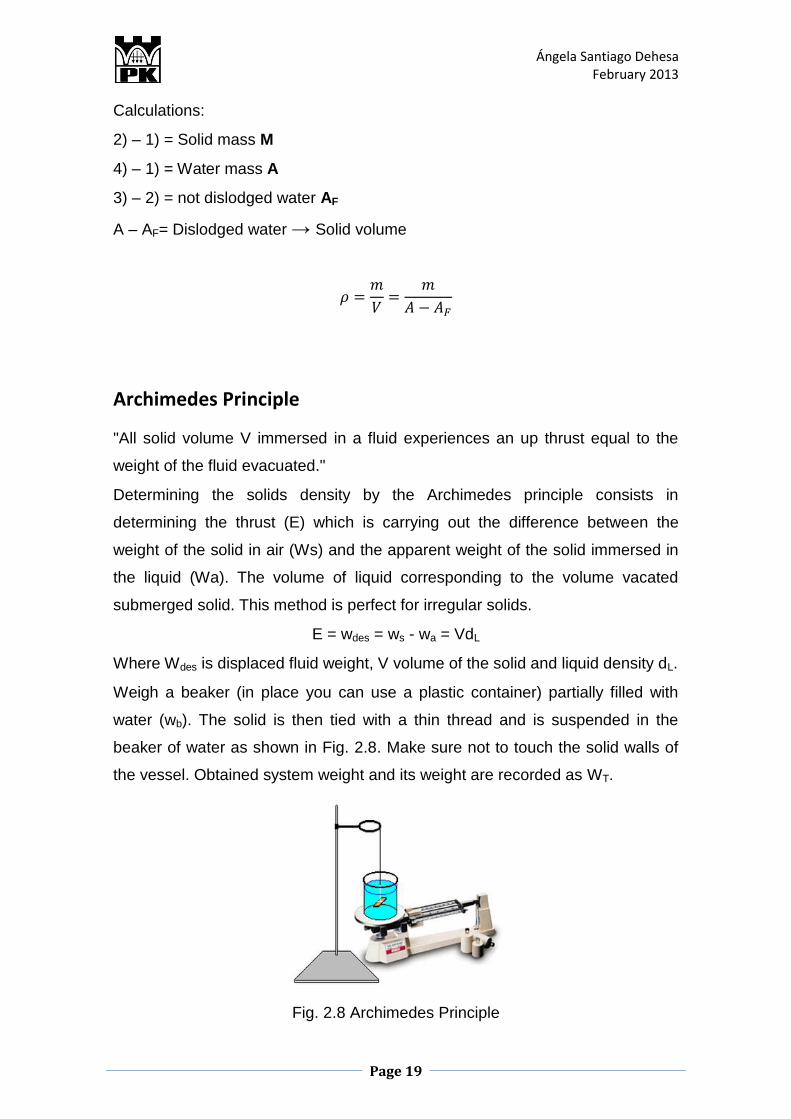
Archimedes Principle
"All solid volume V immersed in a fluid experiences an up thrust equal to the
weight of the fluid evacuated."
Determining the solids density by the Archimedes principle consists in
determining the thrust (E) which is carrying out the difference between the
weight of the solid in air (Ws) and the apparent weight of the solid immersed in
the liquid (Wa). The volume of liquid corresponding to the volume vacated
submerged solid. This method is perfect for irregular solids.
E = wdes = ws - wa = VdL
Where Wdes is displaced fluid weight, V volume of the solid and liquid density dL.
Weigh a beaker (in place you can use a plastic container) partially filled with
water (wb). The solid is then tied with a thin thread and is suspended in the
beaker of water as shown in Fig. 2.8. Make sure not to touch the solid walls of
the vessel. Obtained system weight and its weight are recorded as WT.
Fig. 2.8 Archimedes Principle
Ángela Santiago Dehesa February 2013
Page 20
The rope weight solid supports but does not nullify the push, so that WT equals
the weight of the container with more water thrust (weight of water displaced by
the solid Wdes).
E = wdes = wT - wb = VdL
Bearing in mind that in the above equation, the density can be calculated from
the expression:
Where, if the liquid is water, dL corresponds to 1.00 g / ml.
Test tube method
Is a very common method for irregular solids. The problem that arises is that the
solid has to be quite large, so to properly appreciate the volume change in the
test tube.
The solid was carefully and completely immersed in a beaker containing water
exact volume (VO). Then carefully reads the final volume (VF). The volume of
the solid is the difference:
V = V = Vf - Vo
As found with this method the particle volume by measuring the mass easily
obtain the density of said solid.
Geometrical method
This is a method that can be used only for geometric particles. The particle is to
weigh and get your objects geometrically volume measurement precision.

Ángela Santiago Dehesa February 2013
Page 21
METHODOLOGY OF
WORK
Ángela Santiago Dehesa February 2013
Page 22
3. METHODOLOGY OF WORK
3.1. LABORATORY MATERIAL
3.1.1. GLYCEROL
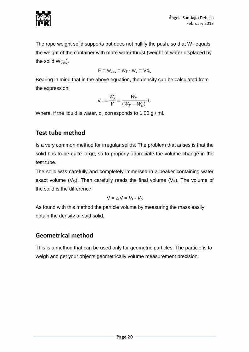
Glycerol (Fig.3.1) is a simple polyol compound. It is a colorless, odorless,
viscous liquid that is widely used in pharmaceutical formulations. Glycerol has
three hydroxyl groups that are responsible for its solubility in water and
its hygroscopic nature. The glycerol backbone is central to all lipids known
as triglycerides. Glycerol is sweet-tasting and of low toxicity.
Fig.3.1 Glycerol’s structure
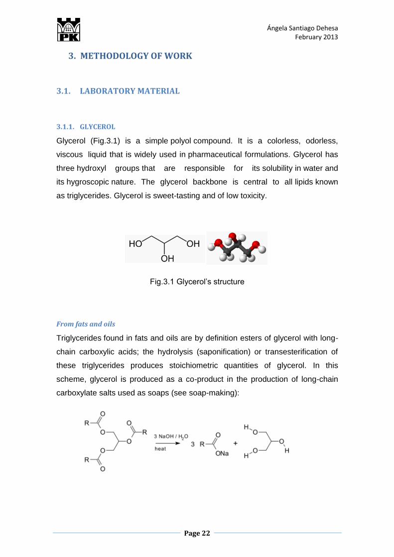
From fats and oils
Triglycerides found in fats and oils are by definition esters of glycerol with long-
chain carboxylic acids; the hydrolysis (saponification) or transesterification of
these triglycerides produces stoichiometric quantities of glycerol. In this
scheme, glycerol is produced as a co-product in the production of long-chain
carboxylate salts used as soaps (see soap-making):
Ángela Santiago Dehesa February 2013
Page 23
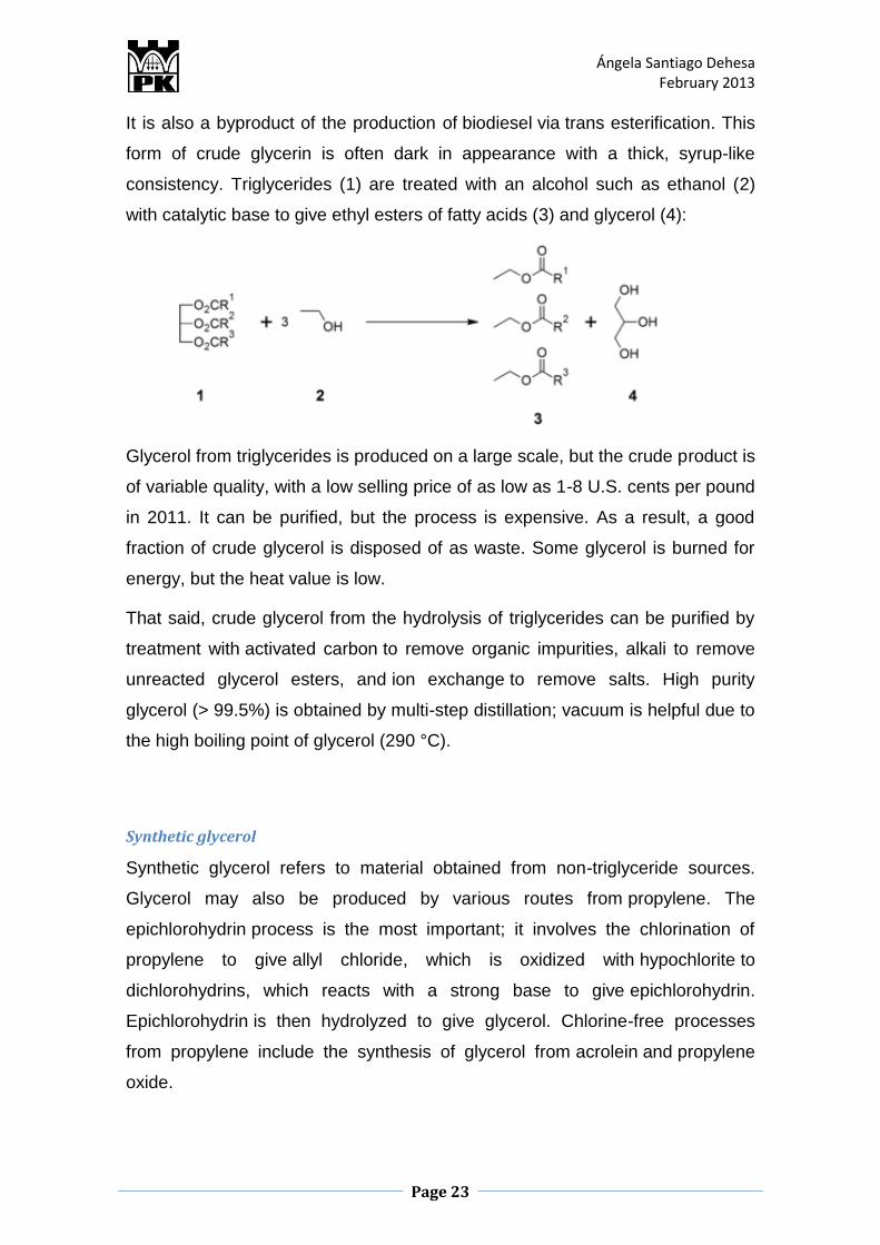
It is also a byproduct of the production of biodiesel via trans esterification. This
form of crude glycerin is often dark in appearance with a thick, syrup-like
consistency. Triglycerides (1) are treated with an alcohol such as ethanol (2)
with catalytic base to give ethyl esters of fatty acids (3) and glycerol (4):
Glycerol from triglycerides is produced on a large scale, but the crude product is
of variable quality, with a low selling price of as low as 1-8 U.S. cents per pound
in 2011. It can be purified, but the process is expensive. As a result, a good
fraction of crude glycerol is disposed of as waste. Some glycerol is burned for
energy, but the heat value is low.
That said, crude glycerol from the hydrolysis of triglycerides can be purified by
treatment with activated carbon to remove organic impurities, alkali to remove
unreacted glycerol esters, and ion exchange to remove salts. High purity
glycerol (> 99.5%) is obtained by multi-step distillation; vacuum is helpful due to
the high boiling point of glycerol (290 °C).
Synthetic glycerol
Synthetic glycerol refers to material obtained from non-triglyceride sources.
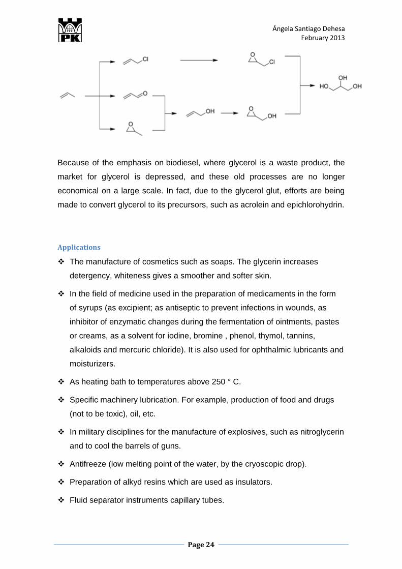
Glycerol may also be produced by various routes from propylene. The
epichlorohydrin process is the most important; it involves the chlorination of
propylene to give allyl chloride, which is oxidized with hypochlorite to
dichlorohydrins, which reacts with a strong base to give epichlorohydrin.
Epichlorohydrin is then hydrolyzed to give glycerol. Chlorine-free processes
from propylene include the synthesis of glycerol from acrolein and propylene
oxide.
Ángela Santiago Dehesa February 2013
Page 24
Because of the emphasis on biodiesel, where glycerol is a waste product, the
market for glycerol is depressed, and these old processes are no longer
economical on a large scale. In fact, due to the glycerol glut, efforts are being
made to convert glycerol to its precursors, such as acrolein and epichlorohydrin.
Applications
The manufacture of cosmetics such as soaps. The glycerin increases
detergency, whiteness gives a smoother and softer skin.
In the field of medicine used in the preparation of medicaments in the form
of syrups (as excipient; as antiseptic to prevent infections in wounds, as
inhibitor of enzymatic changes during the fermentation of ointments, pastes
or creams, as a solvent for iodine, bromine , phenol, thymol, tannins,
alkaloids and mercuric chloride). It is also used for ophthalmic lubricants and
moisturizers.
As heating bath to temperatures above 250 ° C.
Specific machinery lubrication. For example, production of food and drugs
(not to be toxic), oil, etc.
In military disciplines for the manufacture of explosives, such as nitroglycerin
and to cool the barrels of guns.
Antifreeze (low melting point of the water, by the cryoscopic drop).
Preparation of alkyd resins which are used as insulators.
Fluid separator instruments capillary tubes.
Ángela Santiago Dehesa February 2013
Page 25
Paint and varnish industry. Key component varnishes used for finishes. In
some cases, use of 98% glycerol to prepare varnishes electro insulating.
Tobacco industry. Due to the high binding capacity of glycerin, the moisture
can be adjusted in order to eliminate the unpleasant taste and irritating
smoke snuff.
Textiles. Provides elasticity and softness to fabrics.
3.1.2. SOLIDS
For the selection of the particles used in this project I made a selection process,
focusing especially on the particle shape and the relationship of this feature with
its free-fall conditions within a fluid. Thus various types of shapes selected
(analyzed fall within a water pipe):
Shaped boulders half ellipse: not fall straight but sway even colliding with the
walls of the tube.
Angled triangular stones: fall too fast to determine the time, also without fall
straight.
Very angled porous: Some break to hit the tube, and not collide, they lose
small particles as they descend.
Angled with rounded edges: at 10 cm from start turning on themselves and
do tours spiral inside the tube.
Angulated without rounded corners: 90% of them fall in a straight line, also
cross the tube long enough to measure time.
After having selected particles is necessary know various aspects thereof.
Some example might be the projection area, the convexity or length data
provides a microscope, and others are the mass and density.
Obviously, we calculate the mass without any problem with a precision balance.
Furthermore, to calculate the density, it would be easier to calculate the volume
of the same. The first problem we face when having irregular particles, even so,
there are methods described above with which you can calculate this density.
Ángela Santiago Dehesa February 2013
Page 26
The most affordable option in material and the simplicity of the experiment
would be to use the method of the test tube. On the other hand, this method is
discarded without needing an attempt to support this. This is because our
sample particles are too small to observe a change in the height of the liquid
would not be possible to obtain a precise volume.
The next case would be the method to analyze the principle of Archimedes. The
characteristics of the sample are usually good for this method. The problem is
that a university laboratory usually not equipped with a scale with sufficient
precision for it. For this reason, this method is also discarded.
In the case of the pycnometer, nothing seemed to indicate it was not a suitable
method. After the experiment, to perform calculations and get the densities, we
note that these are not correct. Observing this thought, probably the mass of the
particles is too low for this method, or even, the sample is very small, as our
final sample consists of only 12 particles.
Due to the problems encountered during the process, we finally decided to
assume an approximate density for each particle, between 2.5 and 3.3 g/cm3,
due to the material. Thus can calculate each limit velocity by Stokes law.
3.1.3. INSTRUMENTS.
Refractometer
Called refractometry, optical method of determining the speed of propagation of
light in a medium/ compound/ substance/ body, which is directly related to the
density of the medium/ compound/ substance/ body. To use this principle uses
the refraction of light, (which is a fundamental physical property of a substance),
and the measurement range of this principle is called refractive index,
refractometers (Fig. 3.2) are instruments that employ this either refraction
refraction (using several prisms), or the critical angle (prism using only one),
and its primary scale of measurement is the refractive index, from which specific
construct different scales, Brix (sugar), specific gravity, % salts.
Ángela Santiago Dehesa February 2013
Page 27
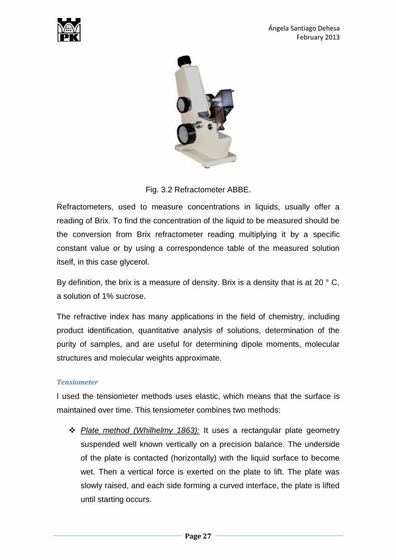
Fig. 3.2 Refractometer ABBE.
Refractometers, used to measure concentrations in liquids, usually offer a
reading of Brix. To find the concentration of the liquid to be measured should be
the conversion from Brix refractometer reading multiplying it by a specific
constant value or by using a correspondence table of the measured solution
itself, in this case glycerol.
By definition, the brix is a measure of density. Brix is a density that is at 20 ° C,
a solution of 1% sucrose.
The refractive index has many applications in the field of chemistry, including
product identification, quantitative analysis of solutions, determination of the
purity of samples, and are useful for determining dipole moments, molecular
structures and molecular weights approximate.
Tensiometer
I used the tensiometer methods uses elastic, which means that the surface is
maintained over time. This tensiometer combines two methods:
Plate method (Whilhelmy 1863): It uses a rectangular plate geometry
suspended well known vertically on a precision balance. The underside
of the plate is contacted (horizontally) with the liquid surface to become
wet. Then a vertical force is exerted on the plate to lift. The plate was
slowly raised, and each side forming a curved interface, the plate is lifted
until starting occurs.
Ángela Santiago Dehesa February 2013
Page 28
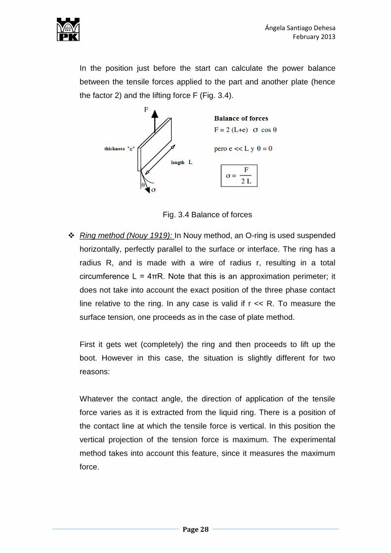
In the position just before the start can calculate the power balance
between the tensile forces applied to the part and another plate (hence
the factor 2) and the lifting force F (Fig. 3.4).
Fig. 3.4 Balance of forces
Ring method (Nouy 1919): In Nouy method, an O-ring is used suspended
horizontally, perfectly parallel to the surface or interface. The ring has a
radius R, and is made with a wire of radius r, resulting in a total
circumference L = 4πR. Note that this is an approximation perimeter; it
does not take into account the exact position of the three phase contact
line relative to the ring. In any case is valid if r << R. To measure the
surface tension, one proceeds as in the case of plate method.
First it gets wet (completely) the ring and then proceeds to lift up the
boot. However in this case, the situation is slightly different for two
reasons:
Whatever the contact angle, the direction of application of the tensile
force varies as it is extracted from the liquid ring. There is a position of
the contact line at which the tensile force is vertical. In this position the
vertical projection of the tension force is maximum. The experimental
method takes into account this feature, since it measures the maximum
force.
Ángela Santiago Dehesa February 2013
Page 29
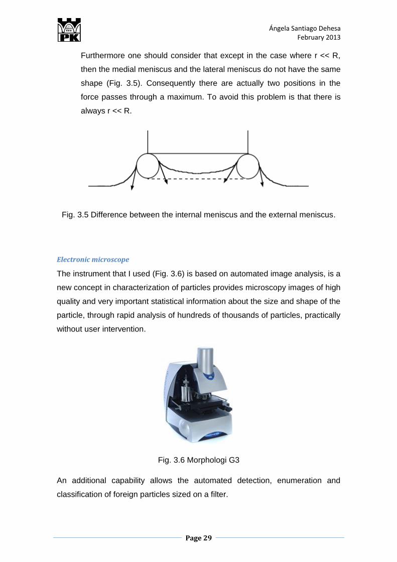
Furthermore one should consider that except in the case where r << R,
then the medial meniscus and the lateral meniscus do not have the same
shape (Fig. 3.5). Consequently there are actually two positions in the
force passes through a maximum. To avoid this problem is that there is
always r << R.
Fig. 3.5 Difference between the internal meniscus and the external meniscus.
Electronic microscope
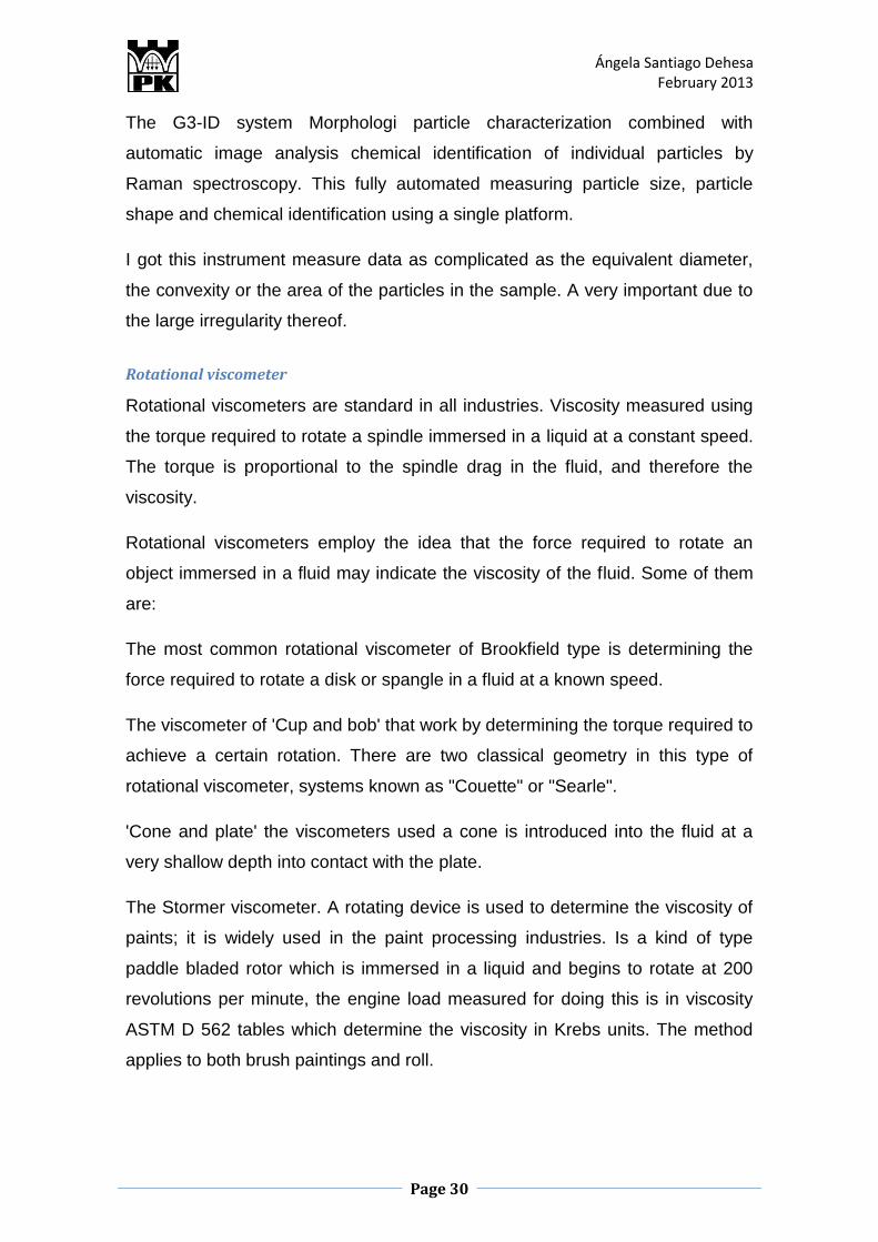
The instrument that I used (Fig. 3.6) is based on automated image analysis, is a
new concept in characterization of particles provides microscopy images of high
quality and very important statistical information about the size and shape of the
particle, through rapid analysis of hundreds of thousands of particles, practically
without user intervention.
Fig. 3.6 Morphologi G3
An additional capability allows the automated detection, enumeration and
classification of foreign particles sized on a filter.
Ángela Santiago Dehesa February 2013
Page 30
The G3-ID system Morphologi particle characterization combined with
automatic image analysis chemical identification of individual particles by
Raman spectroscopy. This fully automated measuring particle size, particle
shape and chemical identification using a single platform.
I got this instrument measure data as complicated as the equivalent diameter,
the convexity or the area of the particles in the sample. A very important due to
the large irregularity thereof.
Rotational viscometer
Rotational viscometers are standard in all industries. Viscosity measured using
the torque required to rotate a spindle immersed in a liquid at a constant speed.
The torque is proportional to the spindle drag in the fluid, and therefore the
viscosity.
Rotational viscometers employ the idea that the force required to rotate an
object immersed in a fluid may indicate the viscosity of the fluid. Some of them
are:
The most common rotational viscometer of Brookfield type is determining the
force required to rotate a disk or spangle in a fluid at a known speed.
The viscometer of 'Cup and bob' that work by determining the torque required to
achieve a certain rotation. There are two classical geometry in this type of
rotational viscometer, systems known as "Couette" or "Searle".
'Cone and plate' the viscometers used a cone is introduced into the fluid at a
very shallow depth into contact with the plate.
The Stormer viscometer. A rotating device is used to determine the viscosity of
paints; it is widely used in the paint processing industries. Is a kind of type
paddle bladed rotor which is immersed in a liquid and begins to rotate at 200
revolutions per minute, the engine load measured for doing this is in viscosity
ASTM D 562 tables which determine the viscosity in Krebs units. The method
applies to both brush paintings and roll.
Ángela Santiago Dehesa February 2013
Page 31
Experiment installation
The installation of the experiment consists of a glass tube about a meter high
and 10.7 cm in diameter. The pipe provided in the bottom of a mesh for
collecting the particles and thereby facilitates the experiment.
Likewise, the tour which measures the time of fall of the particles is determined
by two lines delimiting. These lines serve the function that when the particle
arrives at the first point has already reached its limit speed. The second line is
to delimit the travel 80cm representing the experiment, and thus to calculate the
velocity.
Of course, to the aforementioned speed control, a stopwatch was used analog.
Moreover, for greater control over the temperature has been obtained at which
the temperature fell each particle in each fluid with the help of a thermometer.
3.2. EXPERIMENTAL PROCEDURE
After find out which are the best stones for our experiment, change the tube for
liquid glycerin 85%. At this time I take a larger sample of the type of stones only
I selected (without rounded edges angled) and do a more thorough study on
how such stones and fall exactly as each.
In conducting this experiment thorough we can see that within the particles with
these characteristics (angled flat without rounded edges), there are a
particularly useful for our study, these are the addition to the features mentioned
are quadrilateral. This is because 90% of them fall in a straight line and take a
considerable time in traversing to be measured.
To continue the experiment, glycerol change by 85% to 74% glycerol. Again I
throw stones selected, so I can see the difference in behavior between the two
particles have concentrations.
Concentration of glycerol solutions the measure with a refractometer. As the
first solution (85%) were of unknown concentration, and the second (74%) was
created following the first by adding water. So using the refractometer and a
calculator to the glycerol concentrations get.
Ángela Santiago Dehesa February 2013
Page 32
To find the density of the two liquids, I made use of a Kruss K11 tensiometer.
Data necessary to identify the speed limit using Stokes' law.
The tensiometer gives the measurement of the 85% glycerol has a density of
1.227g/ml (21.5 ° C) and 74% glycerol has a density of 1.191g/ml (21.9 ° C).
After this, we obtain both the viscosity of liquids using a rotational viscometer.
3.3. WORKING TOOLS
For laboratory results, and then to manage, I used the following tools:
Microsoft excel with solver option.
Morphologi software

Ángela Santiago Dehesa February 2013
Page 33
RESULTS
Ángela Santiago Dehesa February 2013
Page 34
4. RESULTS
4.1. PROCESS OF SAMPLE SELECTION
First, we take a very large sample stones of the same material. Fallin observe
their behavior in a water-filled tube, just to preview it on forms that are
disposable from the beginning.
Taking a closer idea about what type of particles are suitable for our
experiment, we establish a distance of 80cm in the water-filled tube. This helps
us to determine a more specific behavior of particles, said particles having
previously separated into seven major groups:
Shaped boulders half ellipse
Rounded angled
Elongated boulders
Triangular beaked
Porous very angled
Angled with rounded edges
Angled beaked
After the previous experiment, we selected only peaked angular particles. Thus,
having a larger sample of a single group, we can divide these into several
subtypes.
Change the water by glycerol. Observe two subtypes that are good candidates
for the experiment. Angled flat square particles and particles with high
convexity.
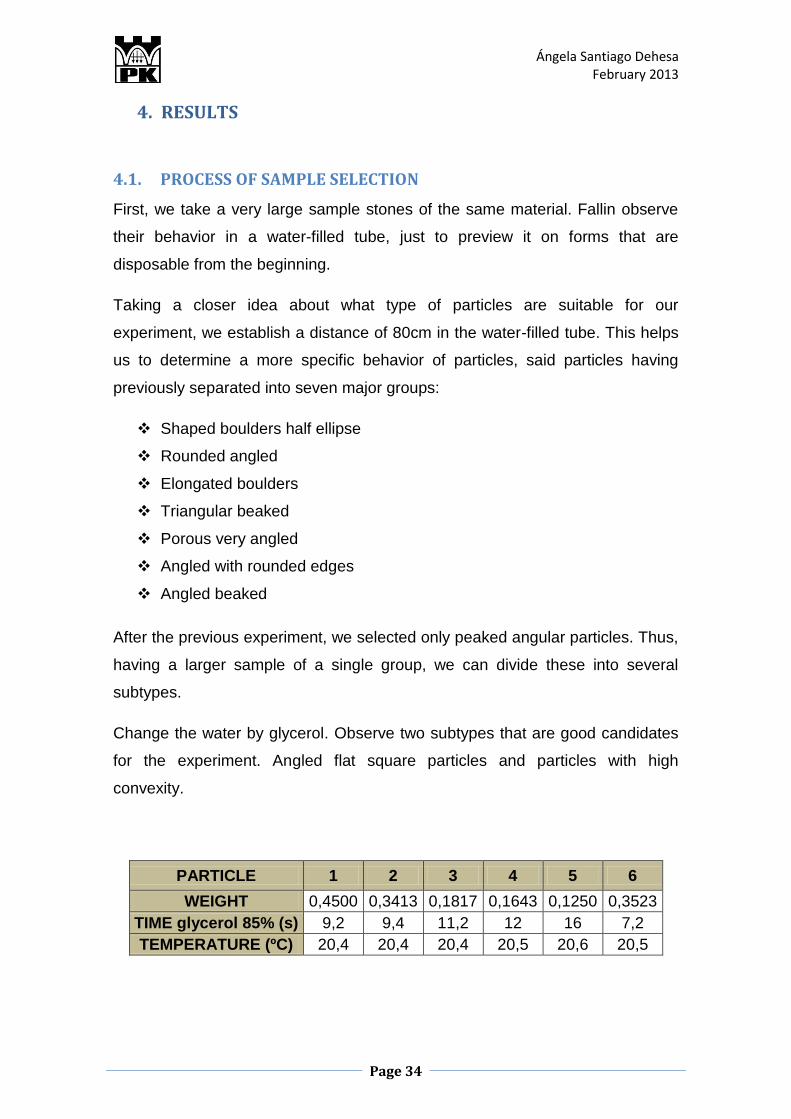
PARTICLE 1 2 3 4 5 6
WEIGHT 0,4500 0,3413 0,1817 0,1643 0,1250 0,3523
TIME glycerol 85% (s) 9,2 9,4 11,2 12 16 7,2
TEMPERATURE (ºC) 20,4 20,4 20,4 20,5 20,6 20,5
Ángela Santiago Dehesa February 2013
Page 35
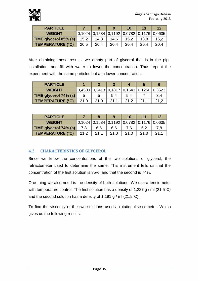
PARTICLE 7 8 9 10 11 12
WEIGHT 0,1024 0,1534 0,1192 0,0782 0,1176 0,0635
TIME glycerol 85% (s) 15,2 14,8 14,6 15,2 13,8 15,2
TEMPERATURE (ºC) 20,5 20,4 20,4 20,4 20,4 20,4
After obtaining these results, we empty part of glycerol that is in the pipe
installation, and fill with water to lower the concentration. Thus repeat the
experiment with the same particles but at a lower concentration.
PARTICLE 1 2 3 4 5 6
WEIGHT 0,4500 0,3413 0,1817 0,1643 0,1250 0,3523
TIME glycerol 74% (s) 5 5 5,4 5,4 7 3,4
TEMPERATURE (ºC) 21,0 21,0 21,1 21,2 21,1 21,2
PARTICLE 7 8 9 10 11 12
WEIGHT 0,1024 0,1534 0,1192 0,0782 0,1176 0,0635
TIME glycerol 74% (s) 7,8 6,6 6,6 7,6 6,2 7,8
TEMPERATURE (ºC) 21,2 21,1 21,0 21,0 21,0 21,1
4.2. CHARACTERISTICS OF GLYCEROL
Since we know the concentrations of the two solutions of glycerol, the
refractometer used to determine the same. This instrument tells us that the
concentration of the first solution is 85%, and that the second is 74%.
One thing we also need is the density of both solutions. We use a tensiometer
with temperature control. The first solution has a density of 1,227 g / ml (21.5°C)
and the second solution has a density of 1,191 g / ml (21.9°C).
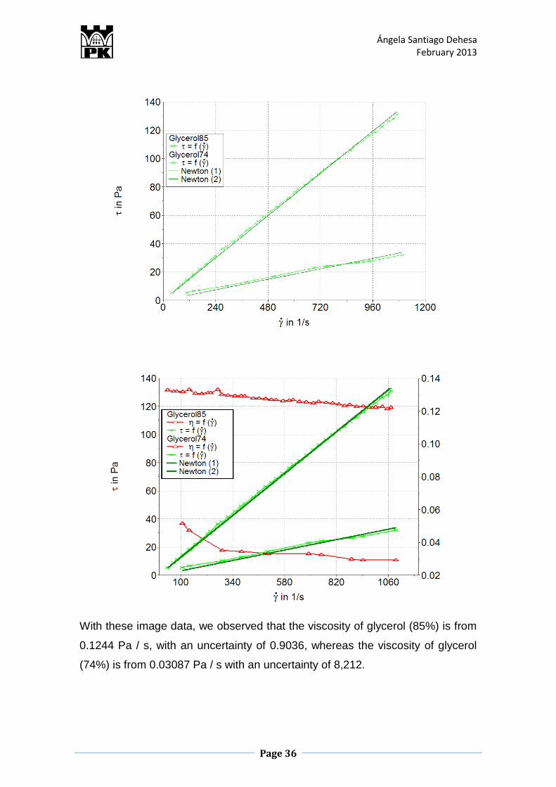
To find the viscosity of the two solutions used a rotational viscometer. Which
gives us the following results:
Ángela Santiago Dehesa February 2013
Page 36
With these image data, we observed that the viscosity of glycerol (85%) is from
0.1244 Pa / s, with an uncertainty of 0.9036, whereas the viscosity of glycerol
(74%) is from 0.03087 Pa / s with an uncertainty of 8,212.
Ángela Santiago Dehesa February 2013
Page 37
4.3. DATA PARTICLES
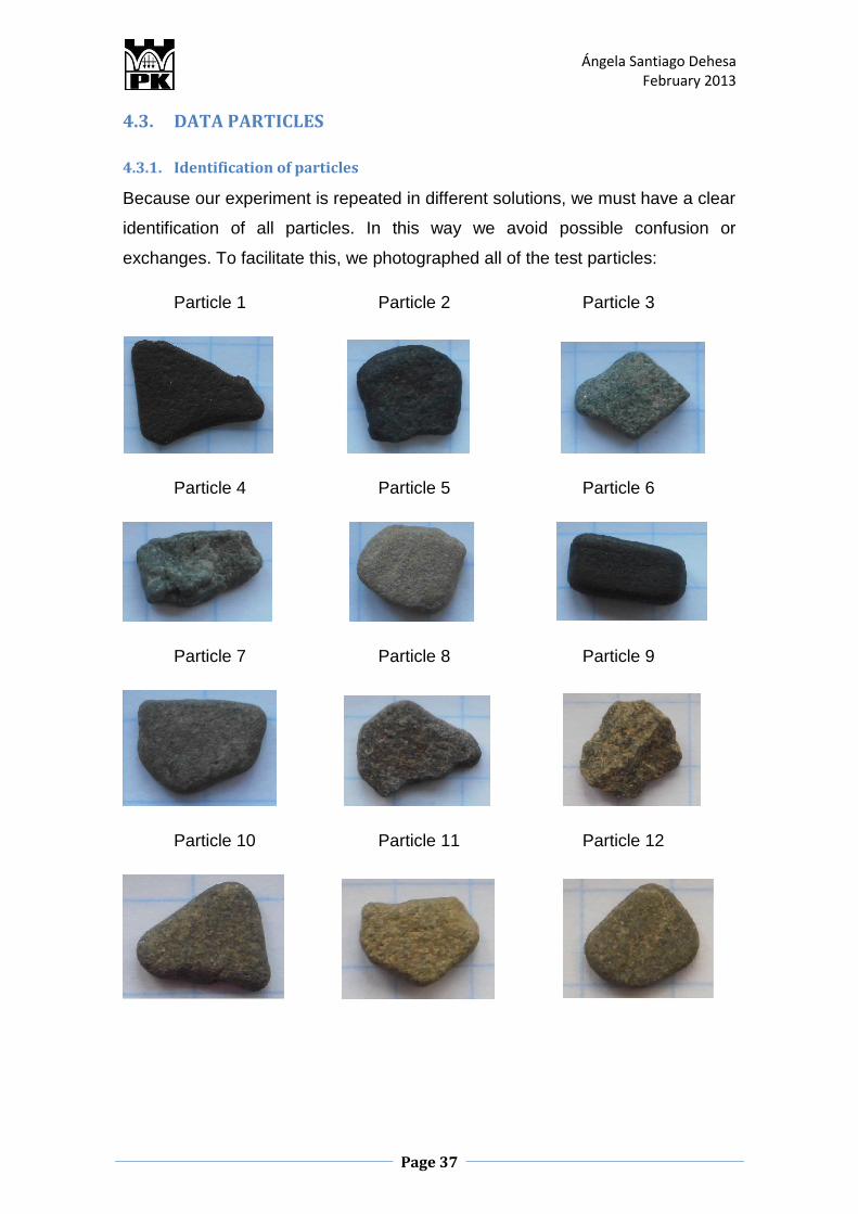
4.3.1. Identification of particles
Because our experiment is repeated in different solutions, we must have a clear
identification of all particles. In this way we avoid possible confusion or
exchanges. To facilitate this, we photographed all of the test particles:
Particle 1 Particle 2 Particle 3
Particle 4 Particle 5 Particle 6
Particle 7 Particle 8 Particle 9
Particle 10 Particle 11 Particle 12
Ángela Santiago Dehesa February 2013
Page 38
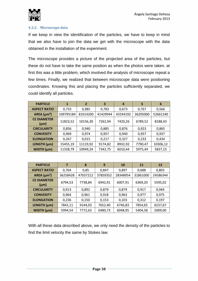
4.3.2. Microscope data
If we keep in view the identification of the particles, we have to keep in mind
that we also have to join the data we get with the microscope with the data
obtained in the installation of the experiment.
The microscope provides a picture of the projected area of the particles, but
these do not have to take the same position as when the photos were taken. at
first this was a little problem, which involved the analysis of microscope repeat a
few times. Finally, we realized that between microscope data were positioning
coordinates. Knowing this and placing the particles sufficiently separated, we
could identify all particles.
PARTICLE 1 2 3 4 5 6
ASPECT RATIO 0,733 0,985 0,783 0,673 0,767 0,566
AREA (µm²) 109795184 81014200 41429944 43244192 36205000 52661240
CE DIAMETER (µm)
11823,52 10156,30 7262,94 7420,26 6789,52 8188,43
CIRCULARITY 0,856 0,940 0,885 0,876 0,923 0,865
CONVEXITY 0,969 0,974 0,957 0,940 0,957 0,937
ELONGATION 0,267 0,015 0,217 0,327 0,233 0,434
LENGTH (µm) 15455,19 11119,92 9174,82 8932,92 7790,47 10306,12
WIDTH (µm) 11328,79 10949,24 7342,75 6010,44 5975,44 5837,15
PARTICLE 7 8 9 10 11 12
ASPECT RATIO 0,764 0,85 0,847 0,897 0,688 0,803
AREA (µm²) 36258428 47037212 37859352 28348954 31861000 24586344
CE DIAMETER (µm)
6794,53 7738,84 6942,91 6007,91 6369,20 5595,02
CIRCULARITY 0,913 0,892 0,879 0,879 0,917 0,944
CONVEXITY 0,964 0,961 0,918 0,963 0,977 0,975
ELONGATION 0,236 0,150 0,153 0,103 0,312 0,197
LENGTH (µm) 7842,11 9144,03 7652,40 6746,83 7854,65 6237,67
WIDTH (µm) 5994,54 7772,63 6480,73 6048,95 5404,58 5009,00
With all these data described above, we only need the density of the particles to
find the limit velocity the same by Stokes law.
Ángela Santiago Dehesa February 2013
Page 39
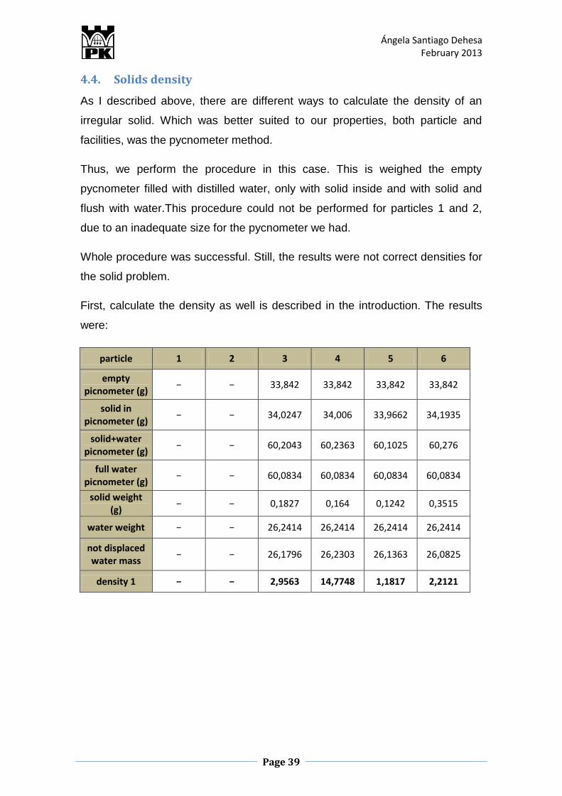
4.4. Solids density
As I described above, there are different ways to calculate the density of an
irregular solid. Which was better suited to our properties, both particle and
facilities, was the pycnometer method.
Thus, we perform the procedure in this case. This is weighed the empty
pycnometer filled with distilled water, only with solid inside and with solid and
flush with water.This procedure could not be performed for particles 1 and 2,
due to an inadequate size for the pycnometer we had.
Whole procedure was successful. Still, the results were not correct densities for
the solid problem.
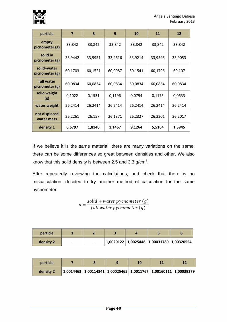
First, calculate the density as well is described in the introduction. The results
were:
particle 1 2 3 4 5 6
empty picnometer (g)
− − 33,842 33,842 33,842 33,842
solid in picnometer (g)
− − 34,0247 34,006 33,9662 34,1935
solid+water picnometer (g)
− − 60,2043 60,2363 60,1025 60,276
full water picnometer (g)
− − 60,0834 60,0834 60,0834 60,0834
solid weight (g)
− − 0,1827 0,164 0,1242 0,3515
water weight − − 26,2414 26,2414 26,2414 26,2414
not displaced water mass
− − 26,1796 26,2303 26,1363 26,0825
density 1 − − 2,9563 14,7748 1,1817 2,2121
Ángela Santiago Dehesa February 2013
Page 40
particle 7 8 9 10 11 12
empty picnometer (g)
33,842 33,842 33,842 33,842 33,842 33,842
solid in picnometer (g)
33,9442 33,9951 33,9616 33,9214 33,9595 33,9053
solid+water picnometer (g)
60,1703 60,1521 60,0987 60,1541 60,1796 60,107
full water picnometer (g)
60,0834 60,0834 60,0834 60,0834 60,0834 60,0834
solid weight (g)
0,1022 0,1531 0,1196 0,0794 0,1175 0,0633
water weight 26,2414 26,2414 26,2414 26,2414 26,2414 26,2414
not displaced water mass
26,2261 26,157 26,1371 26,2327 26,2201 26,2017
density 1 6,6797 1,8140 1,1467 9,1264 5,5164 1,5945
If we believe it is the same material, there are many variations on the same;
there can be some differences so great between densities and other. We also
know that this solid density is between 2.5 and 3.3 g/cm3.
After repeatedly reviewing the calculations, and check that there is no
miscalculation, decided to try another method of calculation for the same
pycnometer.
particle 1 2 3 4 5 6
density 2 − − 1,0020122 1,0025448 1,00031789 1,00320554
particle 7 8 9 10 11 12
density 2 1,0014463 1,00114341 1,00025465 1,0011767 1,00160111 1,00039279
Ángela Santiago Dehesa February 2013
Page 41
Since these results are not correct, the discard. This leads us to think that was
the problem, if at first it seemed that was the best method.
Considering such disparate results obtained with the same data, we think that
maybe the particles have a very low weight for this experiment, and on the other
hand, having a representative sample so small it does not help to find a better
way the problem.
As the objective of our work is to find out the speed limit of particles in our
sample, we assume an average density for all particles, so that we can get an
approximation of that velocity.
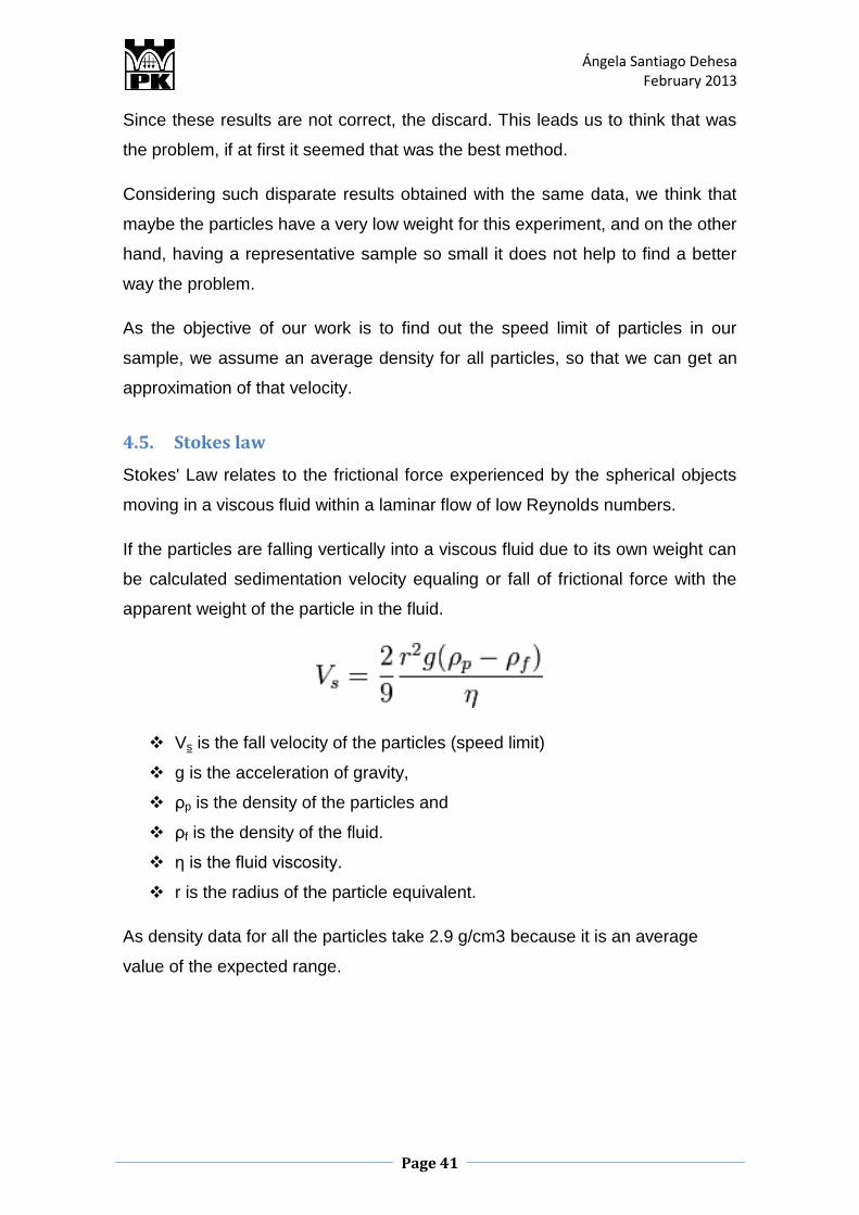
4.5. Stokes law
Stokes' Law relates to the frictional force experienced by the spherical objects
moving in a viscous fluid within a laminar flow of low Reynolds numbers.
If the particles are falling vertically into a viscous fluid due to its own weight can
be calculated sedimentation velocity equaling or fall of frictional force with the
apparent weight of the particle in the fluid.
Vs is the fall velocity of the particles (speed limit)
g is the acceleration of gravity,
ρp is the density of the particles and
ρf is the density of the fluid.
η is the fluid viscosity.
r is the radius of the particle equivalent.
As density data for all the particles take 2.9 g/cm3 because it is an average
value of the expected range.
Ángela Santiago Dehesa February 2013
Page 42
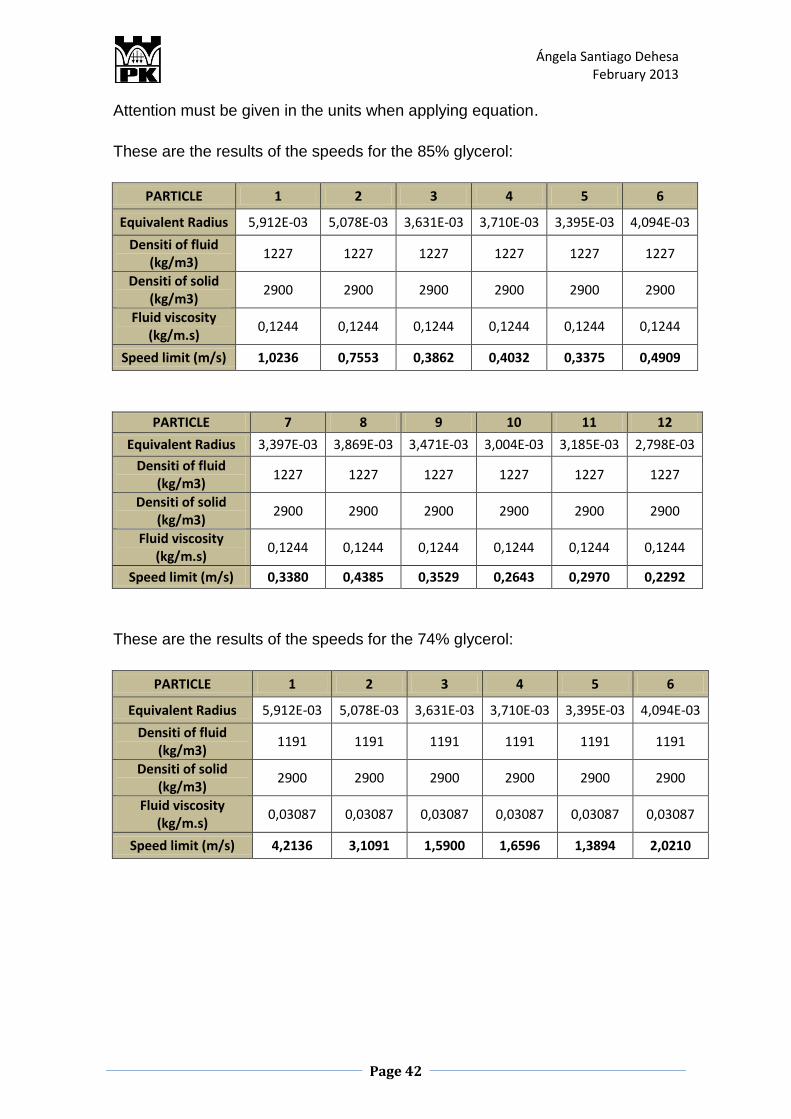
Attention must be given in the units when applying equation.
These are the results of the speeds for the 85% glycerol:
PARTICLE 1 2 3 4 5 6
Equivalent Radius 5,912E-03 5,078E-03 3,631E-03 3,710E-03 3,395E-03 4,094E-03
Densiti of fluid (kg/m3)
1227 1227 1227 1227 1227 1227
Densiti of solid (kg/m3)
2900 2900 2900 2900 2900 2900
Fluid viscosity (kg/m.s)
0,1244 0,1244 0,1244 0,1244 0,1244 0,1244
Speed limit (m/s) 1,0236 0,7553 0,3862 0,4032 0,3375 0,4909
PARTICLE 7 8 9 10 11 12
Equivalent Radius 3,397E-03 3,869E-03 3,471E-03 3,004E-03 3,185E-03 2,798E-03
Densiti of fluid (kg/m3)
1227 1227 1227 1227 1227 1227
Densiti of solid (kg/m3)
2900 2900 2900 2900 2900 2900
Fluid viscosity (kg/m.s)
0,1244 0,1244 0,1244 0,1244 0,1244 0,1244
Speed limit (m/s) 0,3380 0,4385 0,3529 0,2643 0,2970 0,2292
These are the results of the speeds for the 74% glycerol:
PARTICLE 1 2 3 4 5 6
Equivalent Radius 5,912E-03 5,078E-03 3,631E-03 3,710E-03 3,395E-03 4,094E-03
Densiti of fluid (kg/m3)
1191 1191 1191 1191 1191 1191
Densiti of solid (kg/m3)
2900 2900 2900 2900 2900 2900
Fluid viscosity (kg/m.s)
0,03087 0,03087 0,03087 0,03087 0,03087 0,03087
Speed limit (m/s) 4,2136 3,1091 1,5900 1,6596 1,3894 2,0210
Ángela Santiago Dehesa February 2013
Page 43
PARTICLE 7 8 9 10 11 12
Equivalent Radius 3,397E-03 3,869E-03 3,471E-03 3,004E-03 3,185E-03 2,798E-03
Densiti of fluid (kg/m3)
1191 1191 1191 1191 1191 1191
Densiti of solid (kg/m3)
2900 2900 2900 2900 2900 2900
Fluid viscosity (kg/m.s)
0,03087 0,03087 0,03087 0,03087 0,03087 0,03087
Speed limit (m/s) 1,3915 1,8051 1,4529 1,0879 1,2227 0,9435
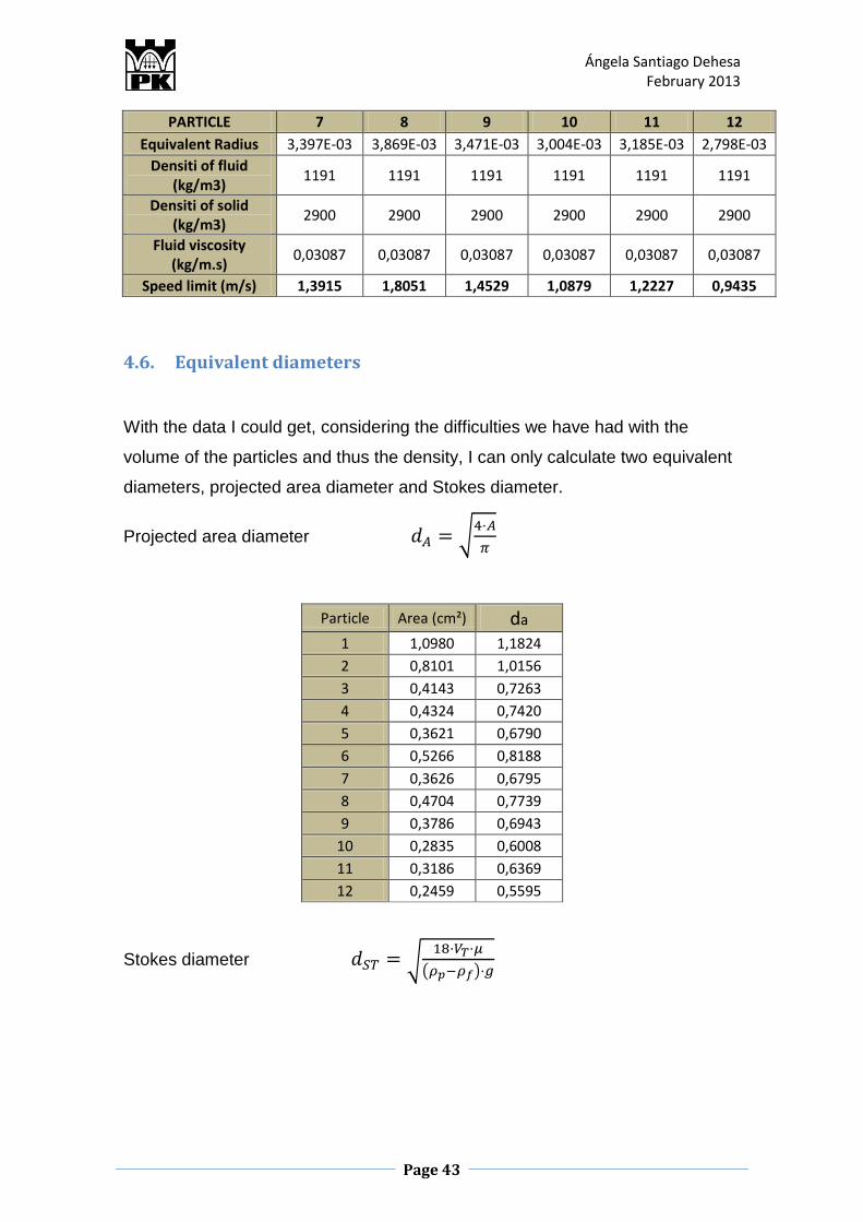
4.6. Equivalent diameters
With the data I could get, considering the difficulties we have had with the
volume of the particles and thus the density, I can only calculate two equivalent
diameters, projected area diameter and Stokes diameter.
Projected area diameter √
Particle Area (cm²) da
1 1,0980 1,1824
2 0,8101 1,0156
3 0,4143 0,7263
4 0,4324 0,7420
5 0,3621 0,6790
6 0,5266 0,8188
7 0,3626 0,6795
8 0,4704 0,7739
9 0,3786 0,6943
10 0,2835 0,6008
11 0,3186 0,6369
12 0,2459 0,5595
Stokes diameter √
( )
Ángela Santiago Dehesa February 2013
Page 44
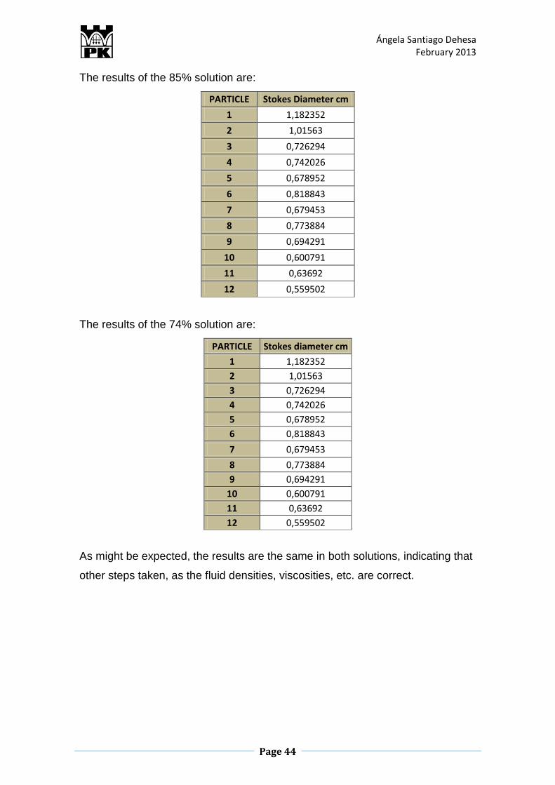
The results of the 85% solution are:
PARTICLE Stokes Diameter cm
1 1,182352
2 1,01563
3 0,726294
4 0,742026
5 0,678952
6 0,818843
7 0,679453
8 0,773884
9 0,694291
10 0,600791
11 0,63692
12 0,559502
The results of the 74% solution are:
PARTICLE Stokes diameter cm
1 1,182352
2 1,01563
3 0,726294
4 0,742026
5 0,678952
6 0,818843
7 0,679453
8 0,773884
9 0,694291
10 0,600791
11 0,63692
12 0,559502
As might be expected, the results are the same in both solutions, indicating that
other steps taken, as the fluid densities, viscosities, etc. are correct.
Ángela Santiago Dehesa February 2013
Page 45
CONCLUSION
Ángela Santiago Dehesa February 2013
Page 46
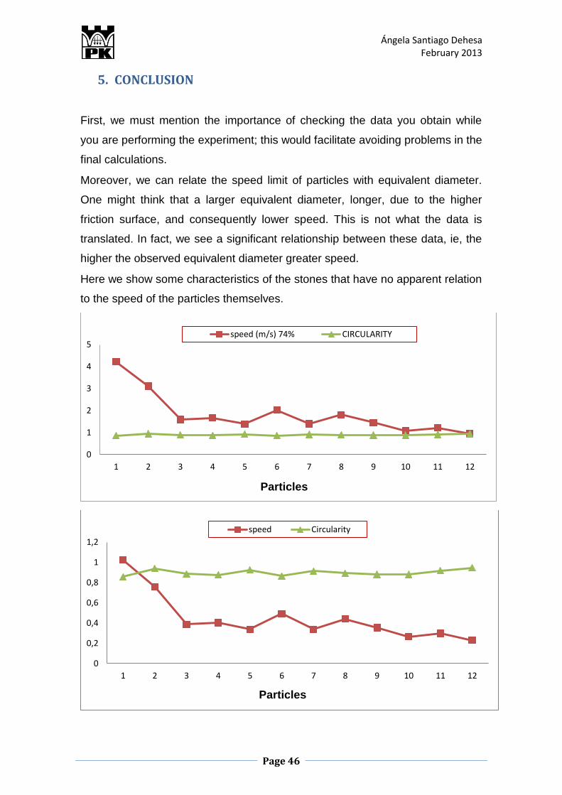
5. CONCLUSION
First, we must mention the importance of checking the data you obtain while
you are performing the experiment; this would facilitate avoiding problems in the
final calculations.
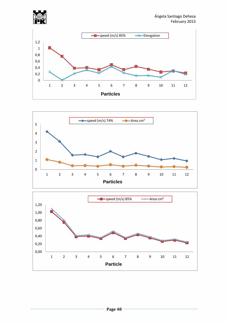
Moreover, we can relate the speed limit of particles with equivalent diameter.
One might think that a larger equivalent diameter, longer, due to the higher
friction surface, and consequently lower speed. This is not what the data is
translated. In fact, we see a significant relationship between these data, ie, the
higher the observed equivalent diameter greater speed.
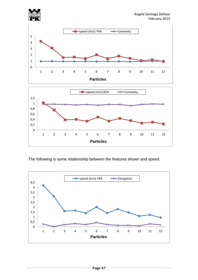
Here we show some characteristics of the stones that have no apparent relation
to the speed of the particles themselves.
0
1
2
3
4
5
1 2 3 4 5 6 7 8 9 10 11 12
Particles
speed (m/s) 74% CIRCULARITY
0
0,2
0,4
0,6
0,8
1
1,2
1 2 3 4 5 6 7 8 9 10 11 12
Particles
speed Circularity
Ángela Santiago Dehesa February 2013
Page 47
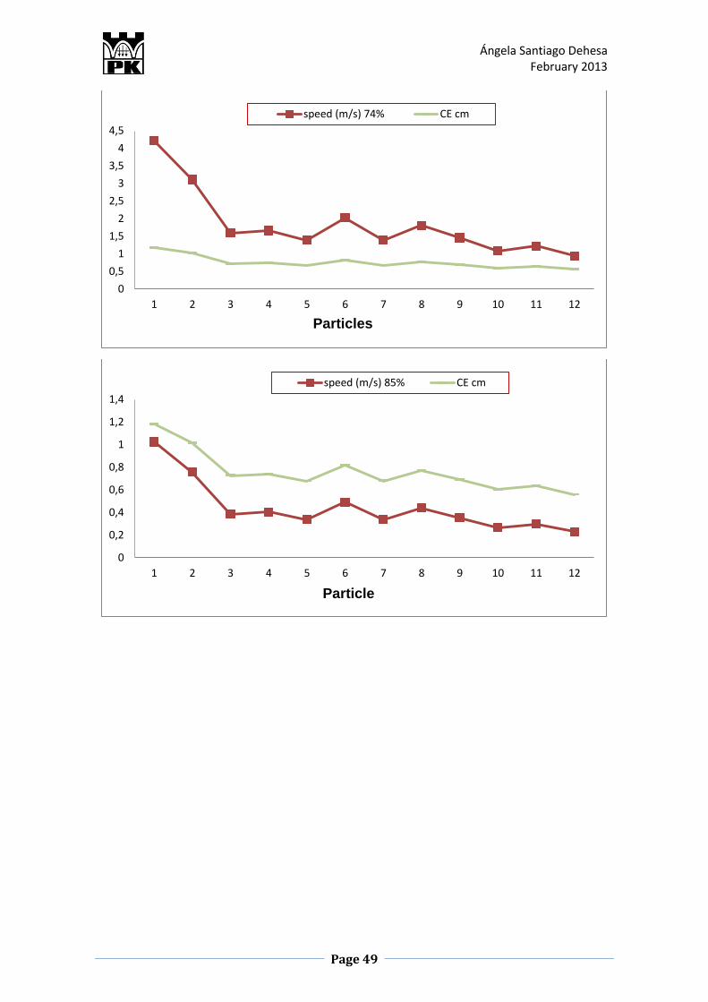
The following is some relationship between the features shown and speed.
0
1
2
3
4
5
1 2 3 4 5 6 7 8 9 10 11 12
Particles
speed (m/s) 74% Convexity
0
0,2
0,4
0,6
0,8
1
1,2
1 2 3 4 5 6 7 8 9 10 11 12
Particles
speed (m/s) 85% Convexity
0
0,5
1
1,5
2
2,5
3
3,5
4
4,5
1 2 3 4 5 6 7 8 9 10 11 12
Particles
speed (m/s) 74% Elongation
Ángela Santiago Dehesa February 2013
Page 48
0
0,2
0,4
0,6
0,8
1
1,2
1 2 3 4 5 6 7 8 9 10 11 12
Particles
speed (m/s) 85% Elongation
0
1
2
3
4
5
1 2 3 4 5 6 7 8 9 10 11 12
Particles
speed (m/s) 74% Area cm²
0,00
0,20
0,40
0,60
0,80
1,00
1,20
1 2 3 4 5 6 7 8 9 10 11 12
Particle
speed (m/s) 85% Area cm²
Ángela Santiago Dehesa February 2013
Page 49
0
0,5
1
1,5
2
2,5
3
3,5
4
4,5
1 2 3 4 5 6 7 8 9 10 11 12
Particles
speed (m/s) 74% CE cm
0
0,2
0,4
0,6
0,8
1
1,2
1,4
1 2 3 4 5 6 7 8 9 10 11 12
Particle
speed (m/s) 85% CE cm

Ángela Santiago Dehesa February 2013
Page 50
BIBLIOGRAPHY
Ángela Santiago Dehesa February 2013
Page 51
6. BIBLIOGRAPHY
Culmann P (1901). Nouveaux réfractomètres. J. Phys. Theor. Appl. 10,
691-704 (1901) http://hal.archives-ouvertes.fr (Data of reference: 17th
January)
Valencien M & Planchaud M. (1923). Titrage rapide des laits anormaux
par la réfractométrie, la catalosimétrie et l’essai à l’acool-alizarine.
http://lait.dairy-journal.org (Date of reference: 4th December) Kerton, Francesca (2009). Alternative solvents for green chemistry. The
Royal Society of Chemistry. Pp 47-64.
Almeida Prieto, S; Blanco Méndez, J; Otero Espinar, FJ. (2007)
Evaluación morfológica de partículas mediante análisis de imagen.
Universidad de Santiago de Compostela. http://www.sciencedirect.com
(Date of reference: 26th November)
Terfous, A. (2006). Measurement and modeling of the settling velocity of
isometric particles. France. Powder Technology. Pp 106-110.
Tsakalakis, K.G., Stamboltzis, G.A. (2000). Prediction of the settling
velocity of irregularly shaped particles. Athens. Elsevier Science Ltd. Pp
349-354.
Henk G. Merkus, (2009). Particle Size Measurements: Fundamentals,
Practice, Quality. Springer. Pp 14-18; 28-36.
Kondrat’ev, A.S., Naumova, E.A. (2002). Calculation of the velocity of
free settling of solid particles in a newtonian liquid. Moscow. Maik Nauka.
Pp 606-610.
Allen, T. (2003). Powder sampling and particle size determination.
Elsevier Science Ltd. Pp 45-52.
Masuda, H. (2006). Powder technology handbook. USA. Taylor &
Francis Group. Pp 3-6; 33-37; 49-51; 125-130.
Calero Cáceres, W. (2010). Síntesis y refinación de biodiesel y glicerina
obtenidos a partir de grasa vegetal. www.monografias.com (Date of
reference: 14th December)
Ángela Santiago Dehesa February 2013
Page 52
Elaboraron: I.Q.I Minerva Juárez Juárez, Dr. Gustavo Valencia del Toro,
M. en C. Juan Ramírez Balderas, I.Q.I. Linaloe Lobato Azuceno, I.B.Q.
Emma Bolaños Valerio, I.B.Q. Pedro Miranda Reyes
http://www.biblioteca.upibi.ipn.mx (Date of reference: 5th January)


![A-001 Rev D · 1) ±0.03 [0.001] for male contact mating diameters. 2) ±0.08 [0.003] for contact termination diameters 3) ±0.13 [0.005] for all diameters 4) ±0.38 [0.015] for all](https://img.pdfslide.us/doc/110x75/5f314a33ef7be24f7f124371/a-001-rev-d-1-003-0001-for-male-contact-mating-diameters-2-008-0003.jpg)


![Online Thévenin Equivalent Determination Using Graphical ... · capability chart [8], estimating maximum power transfer limits [10], and developing an adaptive fault location algorithm](https://img.pdfslide.us/doc/110x75/6085ef21a28e1e7f06416b51/online-thvenin-equivalent-determination-using-graphical-capability-chart-8.jpg)