Embed Size (px)
Citation preview
Universiteit Hasselt Center for Statistics
DETERMINATION OF EFFECTIVE CONCENTRATION 50% (EC50): CASE OF
URANIUM TOXICITY ON CARROT ROOT GROWN IN VITRO CROPPING DEVICE
By: Nanette Renolayan
External Supervisor: Dr. Anne Straczek Internal Supervisor: Dr. Herbert Thijs
Thesis submitted in Partial Fulfilment of the Requirements For the Degree of Master of Science in Applied Statistics
HASSELT, 2006
ii
TABLE OF CONTENTS
Page
I. Introduction …………………………………………….. 1
A. Background of the Study ………………………. 1
B. The Data…………………………………………. 3
II. Methodology ……………………………………………. 4
A. The Log-logistic Model …………………………. 5
B. The Brain-Cousens Model………………………. 7
III. Results ……………………………………………………. 8
A. Exploratory Data Analysis………………………. 8
B. Non-linear Regression Results…………………... 10
IV. Discussion…………………………………………………. 18
References………………………………………………………… 21
Appendix………………………………………………………….. 23
iii
Acknowledgement
The author expresses her gratitude to the researchers of the Belgian Nuclear Research Center (SCK-CEN) Radioecology: Dr. Yves Thiry and Dr. Anne Straczek for providing the data for this thesis.
1
I. INTRODUCTION
A. Background of the study
Uranium toxicity
Uranium is a naturally existing heavy metal found in low levels in rocks, soil and water.
In soil, the normal concentration of Uranium is 300 µg Kg-1 to 11.7 mg Kg-1 (Wikipedia
2006). In exceptional situations, Uranium concentrations in soils can reach tens to
hundreds of milligrams per kg of soil, mostly because of mining and milling ores
activities (Plant et al. 1999). High Uranium concentrations in soil can be toxic and
therefore poses danger to the living organisms.
Because of the undesirable effects of chemicals in soil, the evaluation of their toxicity
becomes paramount. Toxicological tests are conducted, for instance by measuring the
decrease in the rate of soil respiration upon increasing the concentration of heavy metals
(Haanstra and Doelman 1985). Another way is by measuring the growth of terrestrial
plants at increasing chemical concentrations. The part of plant that is first exposed to the
chemical is the root so that in toxicological studies, root length is measured for different
chemical exposures at certain points in time after planting.
EC50
The toxicity of chemicals is commonly expressed in terms of dosage which gives 50%
effect to the response (such as soil respiration or growth of a plant eg. root length)
compared to the control. The effect can be either an increase or a decrease in response.
This is called EC50 or Effective Concentration 50. The latter is also termed Effective
Dose 50(ED50) or RD50 for dosage causing 50% reduction. In animal systems, it is
referred to as LD50, the dosage lethal to 50% of the subjects (Schabenberger et al. 1999).
The EC50 is usually estimated by fitting a log-logistic curve to the data. The model is a
sigmoidal relation on a logarithmic scale rather than linear relation. The logistic model
2
can be applied to dichotomous data such as survival or death and to continuous data for
example weight or biomass, and in terms of length for growth. Several studies of dose-
response in herbicide application experiments have used the log-logistic function to model
dose-response relationships (e.g. Streibig 1980; Laerke and Streibig 1995; Seedfeldt et al.
1995; Hsiao et al. 1996; Sandral et al. 1997 as cited in Schabenberger et al. 1999)
Hormesis
Some studies with growth as response (continuous response) have shown that at some low
concentrations of the toxic substance, growth is stimulated instead of being suppressed.
This stimulus is called hormesis (from the Greek for ‘setting into motion’). A definition of
hormesis derived from Stebbing (1982) is low-dose stimulation followed by higher-dose
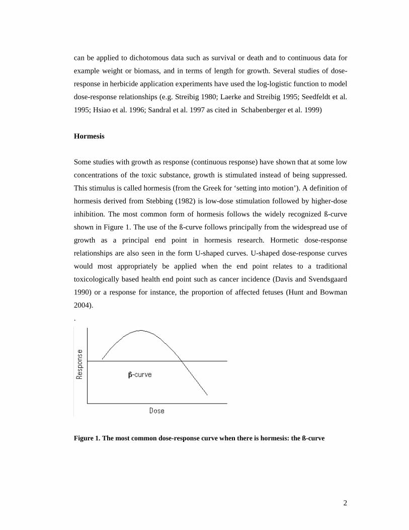
inhibition. The most common form of hormesis follows the widely recognized ß-curve
shown in Figure 1. The use of the ß-curve follows principally from the widespread use of
growth as a principal end point in hormesis research. Hormetic dose-response
relationships are also seen in the form U-shaped curves. U-shaped dose-response curves
would most appropriately be applied when the end point relates to a traditional
toxicologically based health end point such as cancer incidence (Davis and Svendsgaard
1990) or a response for instance, the proportion of affected fetuses (Hunt and Bowman
2004).
.
Figure 1. The most common dose-response curve when there is hormesis: the ß-curve
3
Reference to hormesis can be traced back to Schulz in 1888 who first expressed what is
known today as the Arndt-Schultz law that every toxicant is a stimulant at low levels (
Schabenberger et al. 1999).Several studies have shown that for low dosages of herbicide,
the hormetic effect can occur that raises the average response at low dosages above the
control value(Miller et al. 1962,; Freney, 1965; Wiedman and Appleby, 1972 as cited in
Schabenberger et al. 1999).
An investigation done by Calabrese and Baldwin in 1998 revealed that chemical hormesis
is a reproducible and a relatively common biological phenomenon. Evidence of chemical
hormesis was judged to have occurred in approximately 350 of the 4000 studies
evaluated. Chemical hormesis was observed in a wide range of taxonomic groups and
involved agents representing highly diverse chemical classes, many of which are of
potential environmental relevance. Studies with chemical hormesis use different
biological endpoints. Growth responses were found to be the most prevalent followed by
metabolic effects, longevity, reproductive responses, and survival.
If hormesis occurs, the standard log-logistic model does not fit the data. The usual
practice was to still use the log-logistic model or drop part of the data. A solution was
proposed in 1989 by Brain and Cousens by extending the log-logistic model. This
modification naturally implements hormesis in the log-logistic model (Van Ewijk and
Hoekstra 1993).
B. The Data
The experiment for the study was conducted in the laboratory of Radioecology in
the Belgian Nuclear Research Center (SCK-CEN) in Mol, Belgium. Hairy carrot roots
were grown in an in vitro cropping device containing a gel with different Uranium(U)
concentrations. Eight replicates of carrot root for each U concentration were grown in the
growing medium which contains the following Uranium concentrations: 0, 2.5, 5, 7.5,
10, 15, 20 and 30 mg U per liter. The initial and subsequent days root length (in
centimeter) was measured.
4
The objective of this study is to estimate the EC50 considering the possibility of
occurrence of hormesis.
This thesis is organized as follows. The next section discusses the methodology. Results
are presented in Section 3, followed by the discussion and conclusion in the last section.
II. METHODOLOGY
In order to estimate the EC50, the given data was analyzed by establishing a dose–
response relationship for every time point, that is, at day 0, 2, 6, 9, 13, 16, 20, 27 and 34.
The response variable is in terms root length (in centimeters) and the dose is in milligrams
of Uranium per liter of the growing medium.
Mathematical non-linear models presented in detail below were fitted to the data by non-
linear regression using the procedure PROC NLIN in SAS. Initially, the presence of
hormesis was investigated by fitting the Brain-Cousens model. Two equations of Brain-
Cousens model were fitted to the data. When results reveal the non-significance of
hormesis, the analysis proceeded to fitting the log-logistic models.
The fitted models were verified if the assumption of normality of residuals was met.
Non-linear Regression models
The dose response curves are assumed to follow a non-linear curve specified by the
function f, which are known (the Brain Cousens model or the Log-logistic model). The
function f is a function of dose and a number of parameters. In general, the non- linear
regression models considered in this study can be written as:
iy = ( ) ijixf εα +; , ni ,...,1= j = 1,…m
where ix denotes the ith dose value, jα are the unknown parameters and iε is the error
for the response iy (root length in centimetres in this study). The unknown set of
parameters is different depending on the model assumed (see below). The errors iε are
5
assumed mutually independent and normally distributed N(0, 2σ ). In particular, all
observations have the same variance (homoscedastic).
The parameters are estimated using ordinary least squares (OLS) minimizing
( )∑ −=
n
ixfy ii
1
2
);( α
with respect to the parameters (1α ,…, mα ). Estimations were done using iterative
algorithm Levenberg-Marquardt in PROC NLIN in SAS.
.
A. The Log-logistic model
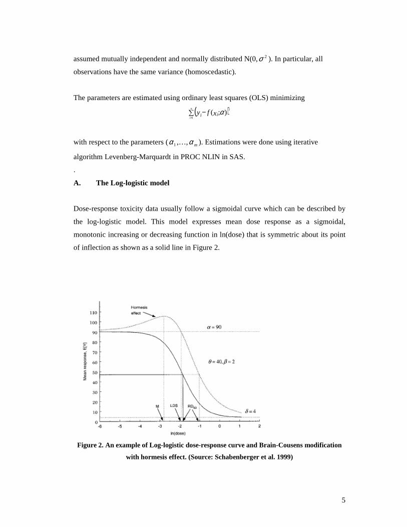
Dose-response toxicity data usually follow a sigmoidal curve which can be described by
the log-logistic model. This model expresses mean dose response as a sigmoidal,
monotonic increasing or decreasing function in ln(dose) that is symmetric about its point
of inflection as shown as a solid line in Figure 2.
Figure 2. An example of Log-logistic dose-response curve and Brain-Cousens modification
with hormesis effect. (Source: Schabenberger et al. 1999)
6
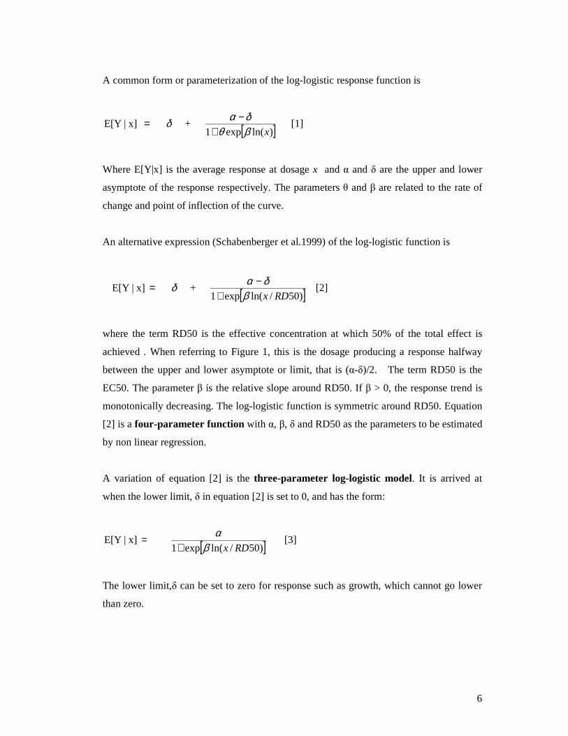
A common form or parameterization of the log-logistic response function is
x]|E[Y = δ + [ ])ln(exp1 xβθδα
+−
[1]
Where E[Y|x] is the average response at dosage x and α and δ are the upper and lower
asymptote of the response respectively. The parameters θ and β are related to the rate of
change and point of inflection of the curve.
An alternative expression (Schabenberger et al.1999) of the log-logistic function is
x]|E[Y = δ + [ ])50/ln(exp1 RDxβδα
+−
[2]
where the term RD50 is the effective concentration at which 50% of the total effect is
achieved . When referring to Figure 1, this is the dosage producing a response halfway
between the upper and lower asymptote or limit, that is (α-δ)/2. The term RD50 is the
EC50. The parameter β is the relative slope around RD50. If β > 0, the response trend is
monotonically decreasing. The log-logistic function is symmetric around RD50. Equation
[2] is a four-parameter function with α, β, δ and RD50 as the parameters to be estimated
by non linear regression.
A variation of equation [2] is the three-parameter log-logistic model. It is arrived at
when the lower limit, δ in equation [2] is set to 0, and has the form:
x]|E[Y = [ ])50/ln(exp1 RDxβα
+ [3]
The lower limit,δ can be set to zero for response such as growth, which cannot go lower
than zero.
7
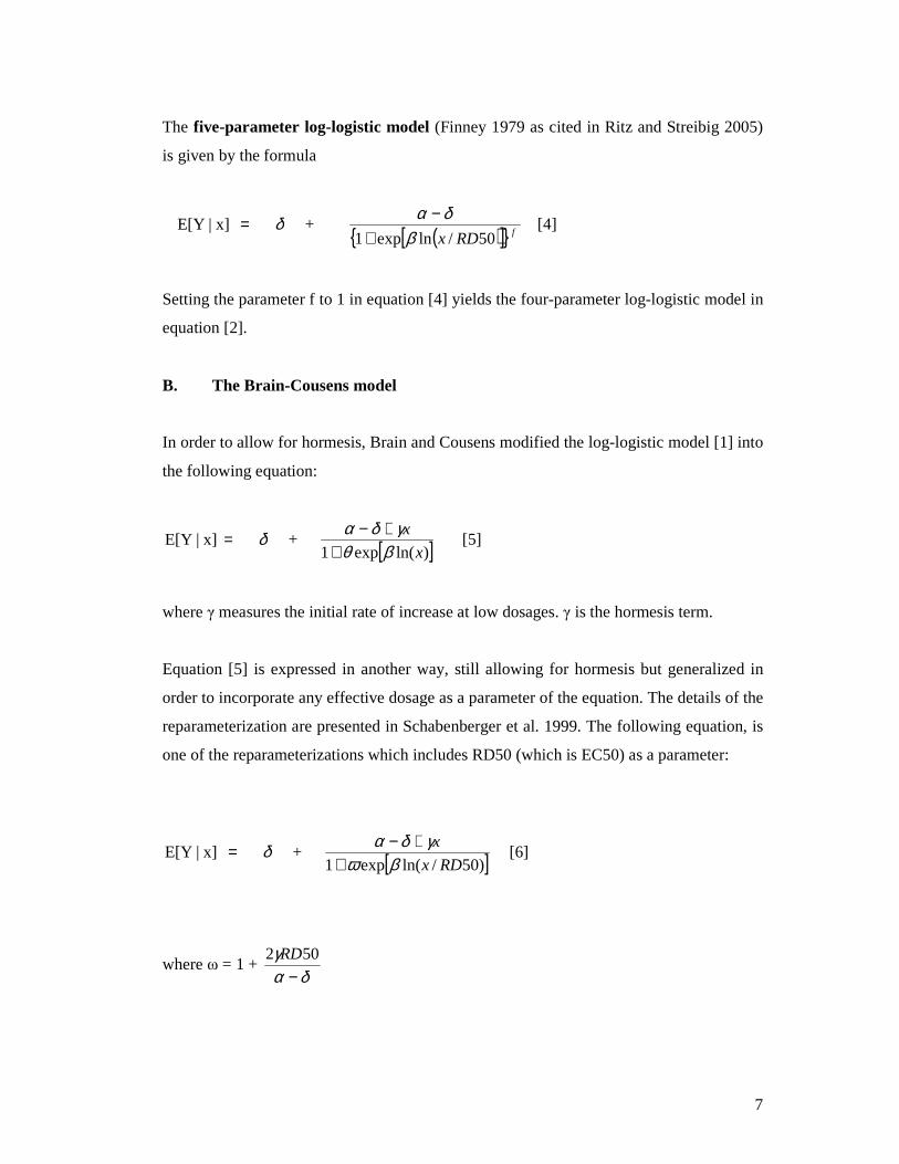
The five-parameter log-logistic model (Finney 1979 as cited in Ritz and Streibig 2005)
is given by the formula
x]|E[Y = δ + ( )[ ]{ } fRDx 50/lnexp1 β
δα+
− [4]
Setting the parameter f to 1 in equation [4] yields the four-parameter log-logistic model in
equation [2].
B. The Brain-Cousens model
In order to allow for hormesis, Brain and Cousens modified the log-logistic model [1] into
the following equation:
x]|E[Y = δ + [ ])ln(exp1 x
x
βθγδα
++−
[5]
where γ measures the initial rate of increase at low dosages. γ is the hormesis term.
Equation [5] is expressed in another way, still allowing for hormesis but generalized in
order to incorporate any effective dosage as a parameter of the equation. The details of the
reparameterization are presented in Schabenberger et al. 1999. The following equation, is
one of the reparameterizations which includes RD50 (which is EC50) as a parameter:
x]|E[Y = δ + [ ])50/ln(exp1 RDx
x
βωγδα
++−
[6]
where ω = 1 + δα
γ−
502 RD
8
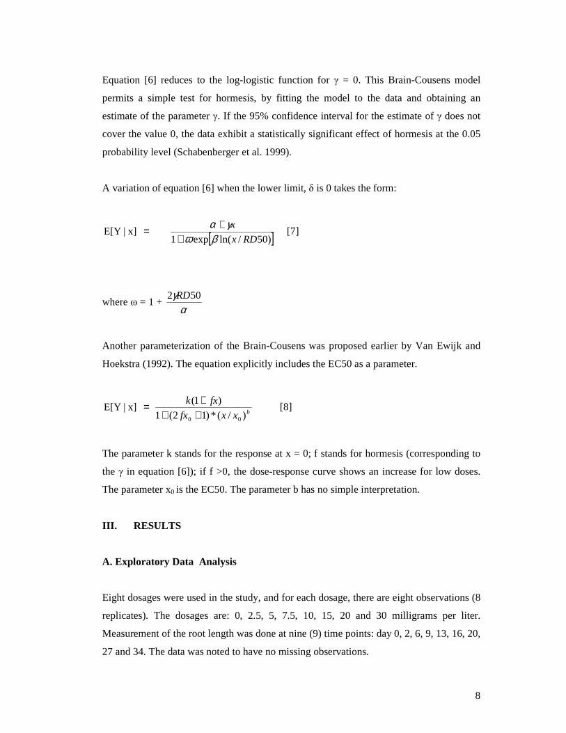
Equation [6] reduces to the log-logistic function for γ = 0. This Brain-Cousens model
permits a simple test for hormesis, by fitting the model to the data and obtaining an
estimate of the parameter γ. If the 95% confidence interval for the estimate of γ does not
cover the value 0, the data exhibit a statistically significant effect of hormesis at the 0.05
probability level (Schabenberger et al. 1999).
A variation of equation [6] when the lower limit, δ is 0 takes the form:
x]|E[Y = [ ])50/ln(exp1 RDx
x
βωγα
++
[7]
where ω = 1 + α
γ 502 RD
Another parameterization of the Brain-Cousens was proposed earlier by Van Ewijk and
Hoekstra (1992). The equation explicitly includes the EC50 as a parameter.
x]|E[Y =bxxfx
fxk
)/(*)12(1
)1(
00 +++
[8]
The parameter k stands for the response at x = 0; f stands for hormesis (corresponding to
the γ in equation [6]); if f >0, the dose-response curve shows an increase for low doses.
The parameter x0 is the EC50. The parameter b has no simple interpretation.
III. RESULTS
A. Exploratory Data Analysis
Eight dosages were used in the study, and for each dosage, there are eight observations (8
replicates). The dosages are: 0, 2.5, 5, 7.5, 10, 15, 20 and 30 milligrams per liter.
Measurement of the root length was done at nine (9) time points: day 0, 2, 6, 9, 13, 16, 20,
27 and 34. The data was noted to have no missing observations.
9
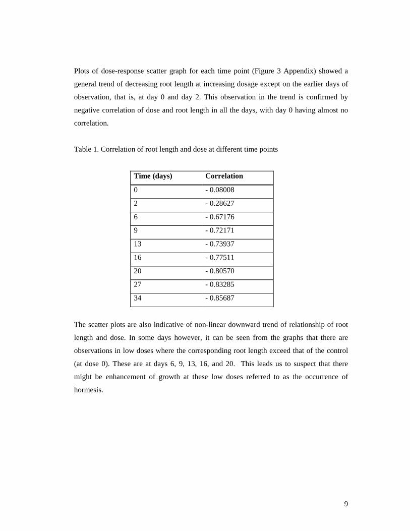
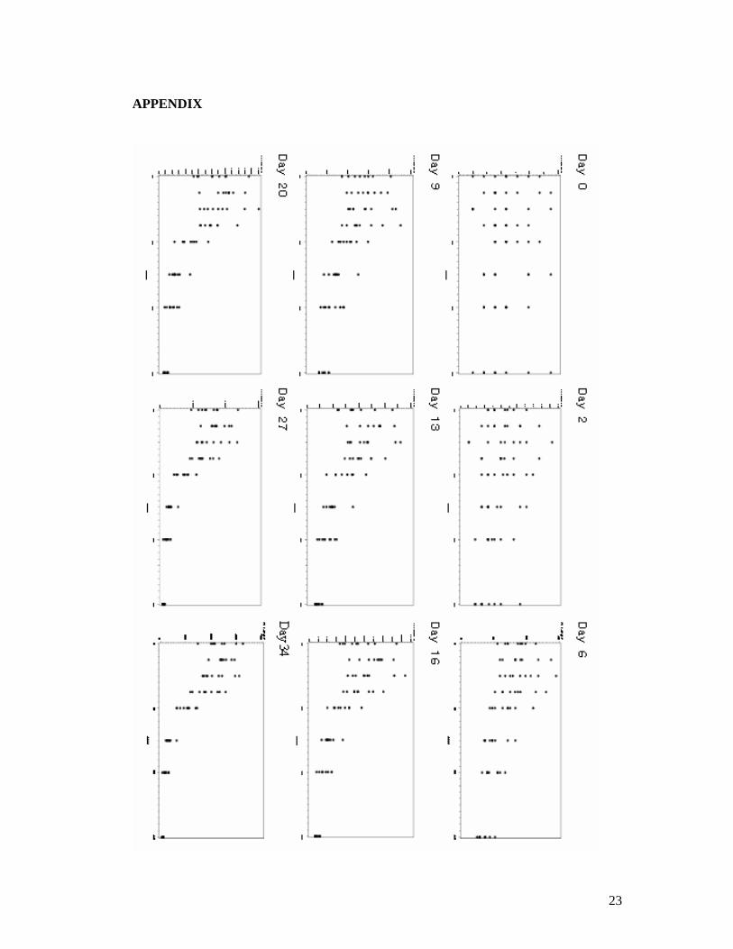
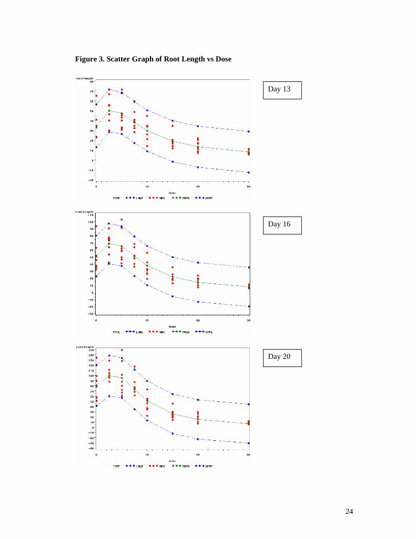
Plots of dose-response scatter graph for each time point (Figure 3 Appendix) showed a
general trend of decreasing root length at increasing dosage except on the earlier days of
observation, that is, at day 0 and day 2. This observation in the trend is confirmed by
negative correlation of dose and root length in all the days, with day 0 having almost no
correlation.
Table 1. Correlation of root length and dose at different time points
Time (days) Correlation
0 - 0.08008
2 - 0.28627
6 - 0.67176
9 - 0.72171
13 - 0.73937
16 - 0.77511
20 - 0.80570
27 - 0.83285
34 - 0.85687
The scatter plots are also indicative of non-linear downward trend of relationship of root
length and dose. In some days however, it can be seen from the graphs that there are
observations in low doses where the corresponding root length exceed that of the control
(at dose 0). These are at days 6, 9, 13, 16, and 20. This leads us to suspect that there
might be enhancement of growth at these low doses referred to as the occurrence of
hormesis.
10
B. Non Linear Regression Results
1. Brain-Cousens models
a. Brain-Cousens model: Schabenberger et al.(1999)
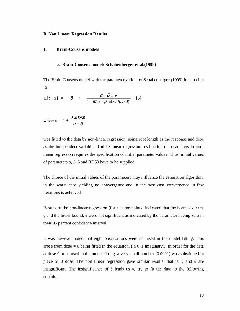
The Brain-Cousens model with the parameterization by Schabenberger (1999) in equation
[6]
x]|E[Y = δ + [ ])50/ln(exp1 RDx
x
βωγδα
++−
[6]
where ω = 1 + δα
γ−
502 RD
was fitted to the data by non-linear regression, using root length as the response and dose
as the independent variable. Unlike linear regression, estimation of parameters in non-
linear regression requires the specification of initial parameter values .Thus, initial values
of parameters α, β, δ and RD50 have to be supplied.
The choice of the initial values of the parameters may influence the estimation algorithm,
in the worst case yielding no convergence and in the best case convergence in few
iterations is achieved.
Results of the non-linear regression (for all time points) indicated that the hormesis term,
γ and the lower bound, δ were not significant as indicated by the parameter having zero in
their 95 percent confidence interval.
It was however noted that eight observations were not used in the model fitting. This
arose from dose = 0 being fitted in the equation. (ln 0 is imaginary). In order for the data
at dose 0 to be used in the model fitting, a very small number (0.0001) was substituted in
place of 0 dose. The non linear regression gave similar results, that is, γ and δ are
insignificant. The insignificance of δ leads us to try to fit the data to the following
equation:
11
x]|E[Y = [ ])50/ln(exp1 RDx
x
βωγα
++
[7]
where ω = 1 + α
γ 502 RD
which is a variation of the previous equation [6], wherein the lower limit term, δ is set to
zero, and δ is not a parameter anymore of the model. Fitting the data with dose = 0
substituted with a very small number (0.0001) resulted in all the four parameters α , β,
RD50 and the hormesis term, γ being significant in days 13, 16 and 20, while for the rest
of the days, the three parameters α, β and RD50 were significant and the hormesis term, γ
not significant. When dose = 0 was not substituted by a very small number, the model
fitting yielded non meaningful results, that is, α was not significant, implying that the
upper bound can be zero which is meaningless for growth data.
Other small values of dose such as 1x10⁻⁷ and 1x10⁻¹⁰ were substituted to dose = 0 to find
out if there is an effect on the estimates. The same results as substituting 0.0001 were
arrived at.
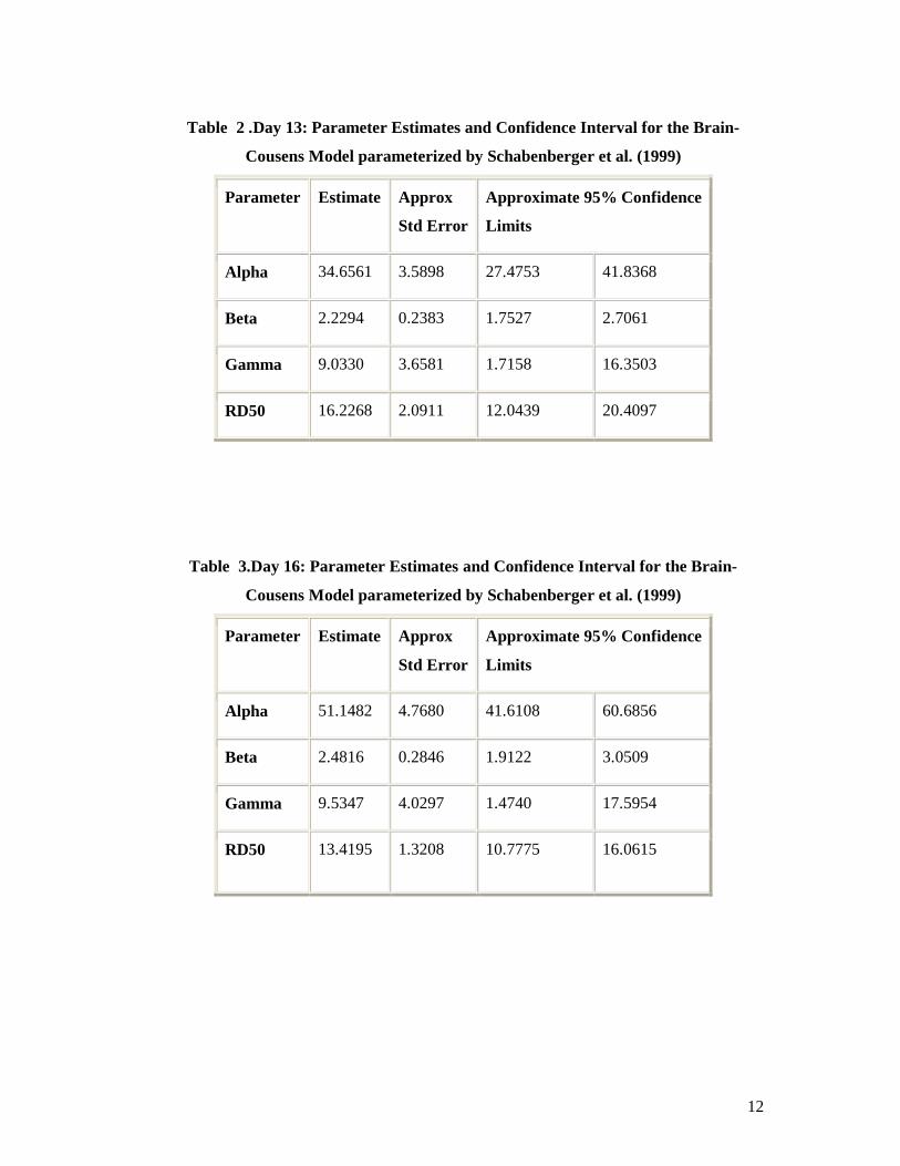
Non-linear models for day 13, day 16 and day 20 use equation [7], with values of the
parameters presented in the following tables:
12
Table 2 .Day 13: Parameter Estimates and Confidence Interval for the Brain-
Cousens Model parameterized by Schabenberger et al. (1999)
Parameter Estimate Approx
Std Error
Approximate 95% Confidence
Limits
Alpha 34.6561 3.5898 27.4753 41.8368
Beta 2.2294 0.2383 1.7527 2.7061
Gamma 9.0330 3.6581 1.7158 16.3503
RD50 16.2268 2.0911 12.0439 20.4097
Table 3.Day 16: Parameter Estimates and Confidence Interval for the Brain-
Cousens Model parameterized by Schabenberger et al. (1999)
Parameter Estimate Approx
Std Error
Approximate 95% Confidence
Limits
Alpha 51.1482 4.7680 41.6108 60.6856
Beta 2.4816 0.2846 1.9122 3.0509
Gamma 9.5347 4.0297 1.4740 17.5954
RD50 13.4195 1.3208 10.7775 16.0615
13
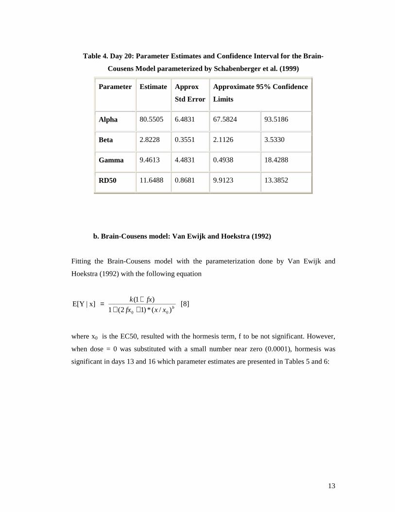
Table 4. Day 20: Parameter Estimates and Confidence Interval for the Brain-
Cousens Model parameterized by Schabenberger et al. (1999)
Parameter Estimate Approx
Std Error
Approximate 95% Confidence
Limits
Alpha 80.5505 6.4831 67.5824 93.5186
Beta 2.8228 0.3551 2.1126 3.5330
Gamma 9.4613 4.4831 0.4938 18.4288
RD50 11.6488 0.8681 9.9123 13.3852
b. Brain-Cousens model: Van Ewijk and Hoekstra (1992)
Fitting the Brain-Cousens model with the parameterization done by Van Ewijk and
Hoekstra (1992) with the following equation
x]|E[Y =bxxfx
fxk
)/(*)12(1
)1(
00 +++
[8]
where x0 is the EC50, resulted with the hormesis term, f to be not significant. However,
when dose = 0 was substituted with a small number near zero (0.0001), hormesis was
significant in days 13 and 16 which parameter estimates are presented in Tables 5 and 6:
14
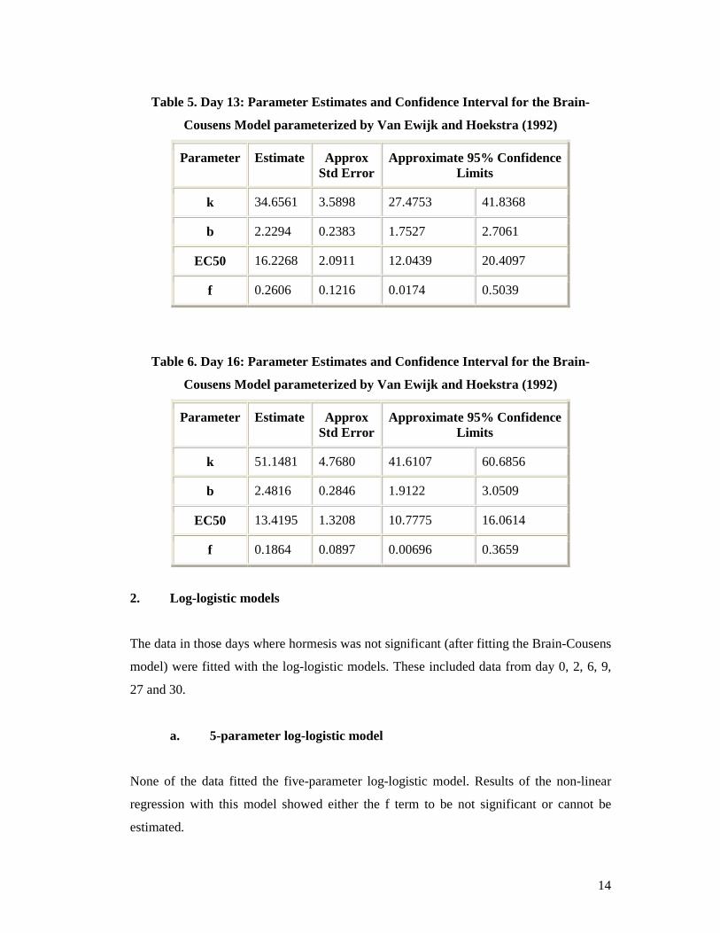
Table 5. Day 13: Parameter Estimates and Confidence Interval for the Brain-
Cousens Model parameterized by Van Ewijk and Hoekstra (1992)
Parameter Estimate Approx Std Error
Approximate 95% Confidence Limits
k 34.6561 3.5898 27.4753 41.8368
b 2.2294 0.2383 1.7527 2.7061
EC50 16.2268 2.0911 12.0439 20.4097
f 0.2606 0.1216 0.0174 0.5039
Table 6. Day 16: Parameter Estimates and Confidence Interval for the Brain-
Cousens Model parameterized by Van Ewijk and Hoekstra (1992)
Parameter Estimate Approx Std Error
Approximate 95% Confidence Limits
k 51.1481 4.7680 41.6107 60.6856
b 2.4816 0.2846 1.9122 3.0509
EC50 13.4195 1.3208 10.7775 16.0614
f 0.1864 0.0897 0.00696 0.3659
2. Log-logistic models
The data in those days where hormesis was not significant (after fitting the Brain-Cousens
model) were fitted with the log-logistic models. These included data from day 0, 2, 6, 9,
27 and 30.
a. 5-parameter log-logistic model
None of the data fitted the five-parameter log-logistic model. Results of the non-linear
regression with this model showed either the f term to be not significant or cannot be
estimated.
15
b. 4-parameter log-logistic model
Only one data set, that is, Day 9 fitted the four-parameter log-logistic model. Taking the
form of equation [2], the model for Day 9 is:
x]|E[Y = δ + [ ])50/ln(exp1 RDxβδα
+−
[2]
where the parameter estimates are in Table 7:
Table 7. Day 9: Parameter Estimates and Confidence Intervals using four-parameter
log-logistic model
Parameter Estimate Approx
Std Error
Approximate 95% Confidence
Limits
alpha 27.5435 1.5173 24.5086 30.5785
delta 8.0027 2.9376 2.1265 13.8788
beta 3.9448 1.8102 0.3239 7.5658
RD50 11.9733 1.7801 8.4126 15.5340
c. 3-parameter log-logistic model
Four data sets: Day 6, Day 9, Day 27 and Day 34 fitted into the three-parameter log-
logistic model, with the following equation:
x]|E[Y = [ ])50/ln(exp1 RDxβα
+ [3]
where the parameter estimates are in Tables 8 , 9 , 10 and 11 :
16
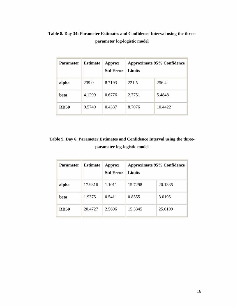
Table 8. Day 34: Parameter Estimates and Confidence Interval using the three-
parameter log-logistic model
Table 9. Day 6. Parameter Estimates and Confidence Interval using the three-
parameter log-logistic model
Parameter Estimate Approx
Std Error
Approximate 95% Confidence
Limits
alpha 17.9316 1.1011 15.7298 20.1335
beta 1.9375 0.5411 0.8555 3.0195
RD50 20.4727 2.5696 15.3345 25.6109
Parameter Estimate Approx
Std Error
Approximate 95% Confidence
Limits
alpha 239.0 8.7193 221.5 256.4
beta 4.1299 0.6776 2.7751 5.4848
RD50 9.5749 0.4337 8.7076 10.4422
17
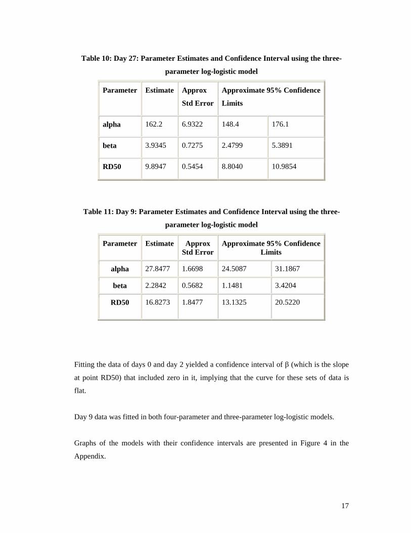
Table 10: Day 27: Parameter Estimates and Confidence Interval using the three-
parameter log-logistic model
Parameter Estimate Approx
Std Error
Approximate 95% Confidence
Limits
alpha 162.2 6.9322 148.4 176.1
beta 3.9345 0.7275 2.4799 5.3891
RD50 9.8947 0.5454 8.8040 10.9854
Table 11: Day 9: Parameter Estimates and Confidence Interval using the three-
parameter log-logistic model
Parameter Estimate Approx Std Error
Approximate 95% Confidence Limits
alpha 27.8477 1.6698 24.5087 31.1867
beta 2.2842 0.5682 1.1481 3.4204
RD50 16.8273 1.8477 13.1325 20.5220
Fitting the data of days 0 and day 2 yielded a confidence interval of β (which is the slope
at point RD50) that included zero in it, implying that the curve for these sets of data is
flat.
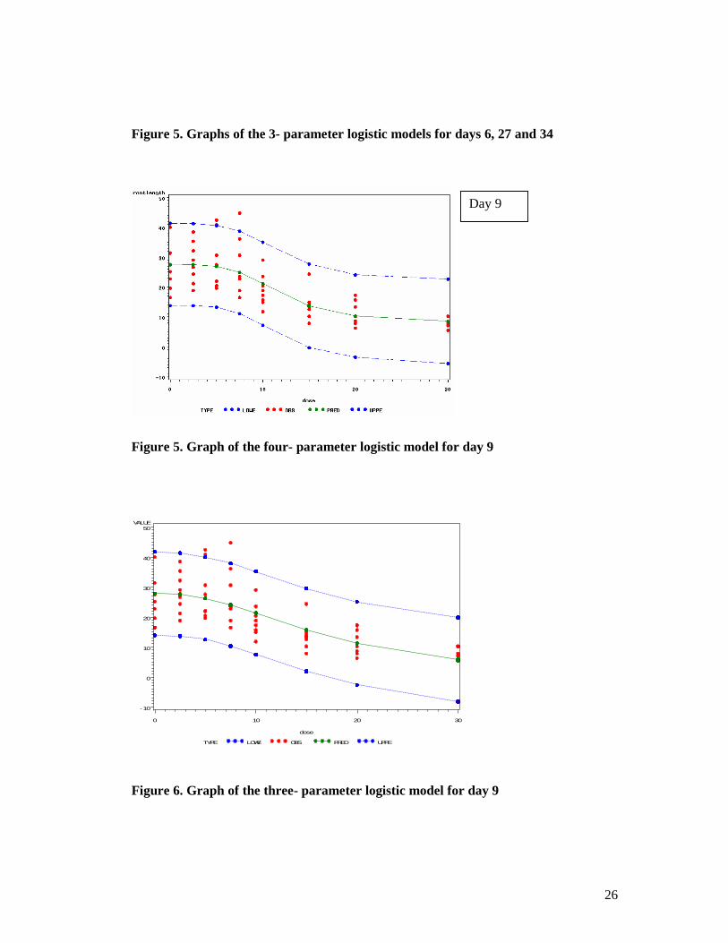
Day 9 data was fitted in both four-parameter and three-parameter log-logistic models.
Graphs of the models with their confidence intervals are presented in Figure 4 in the
Appendix.
18
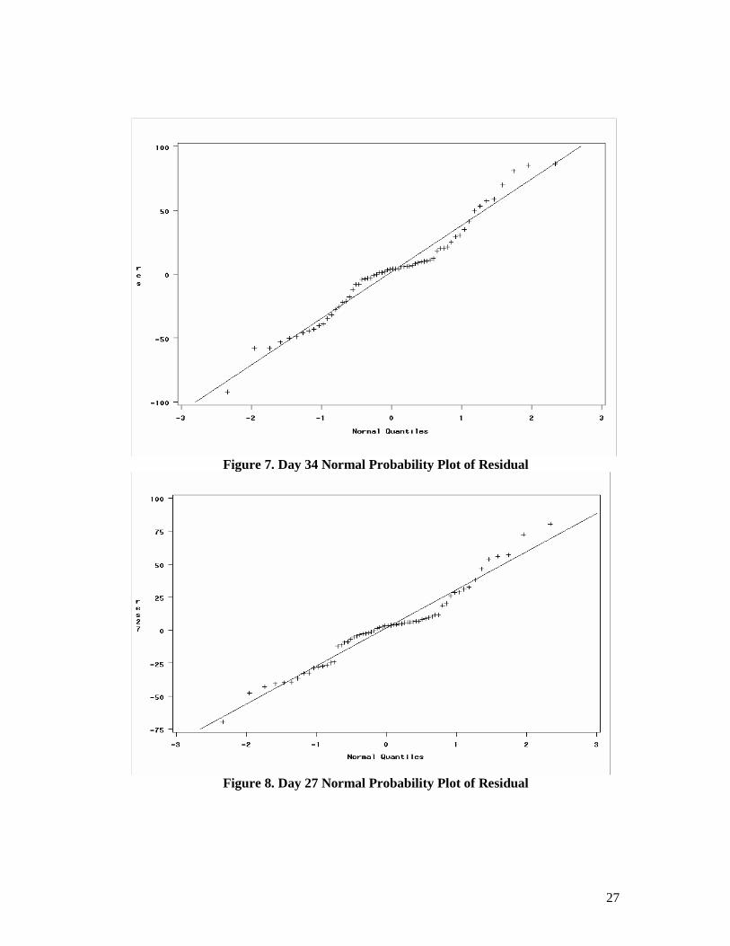
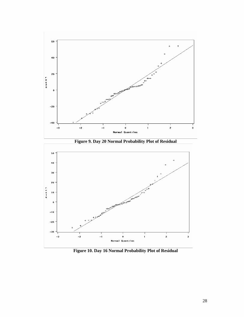
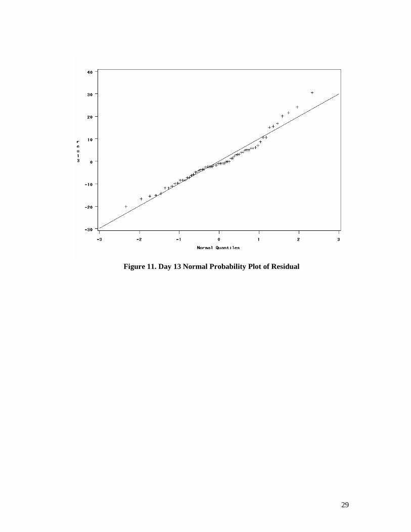
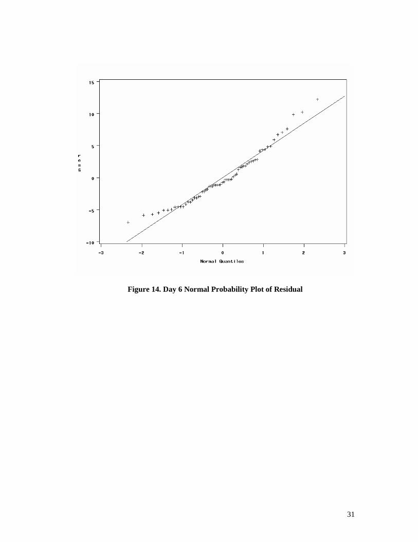
Results of Diagnostics
The normal probability plots of residuals for each day-model are shown in Figures 7 to 14
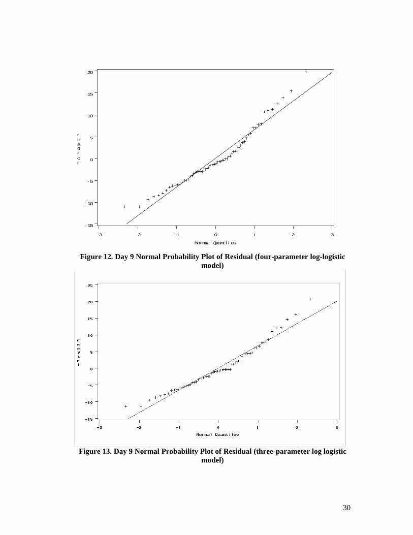
in the Appendix. No serious departures from normality can be seen from the graphs.
Comparing the normal probability plots for the two models for day 9, the three-parameter
model appears to be better than the four-parameter model. The three-parameter model for
day 9 is therefore adapted as the final model.
IV. DISCUSSION AND CONCLUSION
The study investigates whether there was an occurrence of growth stimulation at low
dosage (called hormesis) of Uranium and estimate the EC50. To answer these research
questions, the data was analized for each time point(day) by establishing a dose-response
relationship for each time point with the use of non linear regression.
Fitting the Brain-Cousens model into the data was deemed appropriate because this
allows for simultaneous investigation of the statistical significance of hormesis, and the
estimation of EC50 (and its confidence interval), because these two are included as
parameters of the equation. Disregarding hormesis may lead to erroneous calculation of
the EC50.
There were two parameterizations of the Brain-Cousens models tried in this study in order
to validate if the same conclusions regarding the occurrence of hormesis and the EC50
estimates are arrived at. It attempts to verify whether different parameterizations would
result to the same conclusions. In this study, same conclusions are arrived at for most of
the time points (days), but different conclusion at one time point, that is at day 20.The use
of the Brain-Cousens model parameterized by Schabenberger, et al. for Day 20 data led to
a conclusion of significant hormesis but using the Brain-Cousens model parameterized by
Van Ewijk and Hoekstra resulted to the opposite conclusion (ie. not significant hormesis).
19
This raises the question whether different parameterization may lead to differing
conclusions. The estimates of EC50 however are equal even at day 20.
In the course of doing the non linear regression in this study, it was experienced that the
starting values supplied for the parameters can affect convergence, at one time may not
converge and on other times may converge after just a few iterations. Therefore, caution
in supplying the starting values of the parameters is suggested.
It was also noticed that when some values at the lower doses, particularly at dose 0 were
not included in the modelling, lead to the conclusion of no hormesis. When dose 0 was
substituted with a very small number (therefore including the observations in the
analysis), lead to the conclusion of significant hormesis at some time points, particularly
at days 13, 16 and 20. It can be seen from this that the observations at the control (dose 0)
are very important in the analysis. As a recomendation, it would be helpful to include
some smaller doses in the design of the experiment to be able to detect hormesis.
From the results, it can be seen that there was no hormesis in the earlier days (day 0, day 6
and day 9) and in the later days (day 27 and 34). Hormesis is observed in days 13, 16 and
20. It implies that it takes a few days to pass before hormesis is observed, then hormesis
ceases after sometime.
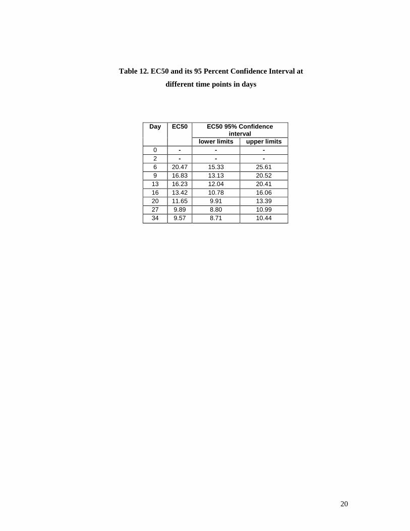
A summary of the EC50 and its 95% confidence interval at each time point is in Table 12.
20
Table 12. EC50 and its 95 Percent Confidence Interval at
different time points in days
EC50 95% Confidence
interval Day EC50
lower limits upper limits 0 - - - 2 - - - 6 20.47 15.33 25.61 9 16.83 13.13 20.52 13 16.23 12.04 20.41 16 13.42 10.78 16.06 20 11.65 9.91 13.39 27 9.89 8.80 10.99 34 9.57 8.71 10.44
21
REFERENCES
Calabrese E. & Baldwin L. Hormesis as a Biological Hypothesis. Retrieved May 17,
2006. http://www.ehponline.org/members/1998/Suppl-1/357-362calabrese/full.html
Davis JM, Svendsgaard DJ.(1990). U-shaped dose-response curves: their occurrence and
implications for risk assessment. J Toxicol Environ Health 30, 71-83.
Haanstra, L., Doelman, P. & Oude Voshaar J.H. (1985). The Use of Sigmoidal Dose
Response Curves in Soil Ecotoxicological Research. Plant and Soil, 84, 293-297.
Hunt D. & Bowman, D.(2004). A Parametric Model for Detecting Hormetic Effects in
Developmental Toxicity Studies. Risk Analysis, 24, 65-72.
Plant, J., Simpson, P. Smith, B., Windley, B.(1999). Uranium ore deposits-products of the
radioactive earth. In : Burns, P., Finch, R.(Eds.), Uranium: Mineralogy, geochemistry and
the environment. Review in Mineralogy. Mineralogy Society of America, Washington
DC, pp.225-319.
Ritz, C. & Streibig, J. (2005). Bioassay Analysis using R. Journal of Statistical Software,
12, 1-22.
Schabenberger, O., Tharp, B., Kells, J. & Penner, D. (1999). Statistical Tests for
Hormesis and Effective Dosages in Herbicide Dose Response. Agronomy Journal, 91,
713-721.
22
Stebbing ,ARD. (1982). Hormesis--the stimulation of growth by low levels of inhibitors.
Sci Total Environ 22,213-234.
Van Ewijk, P.H. & Hoekstra J. A. (1993). Calculation of the EC50 and Its Confidence
Interval When Subtoxic Stimulus is Present. Ecotoxicology and Environmental Safety, 25,
25-32.
Wikipedia (2006). Uranium in the Environment. Retrieved October 13, 2006 from
http://en.wikipedia.org/wiki/Uranium_in_the_environment
23
APPENDIX
24
Figure 3. Scatter Graph of Root Length vs Dose
Day 13
Day 16
Day 20
25
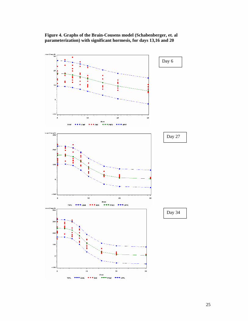
Figure 4. Graphs of the Brain-Cousens model (Schabenberger, et. al parameterization) with significant hormesis, for days 13,16 and 20
Day 6
Day 27
Day 34
26
Figure 5. Graphs of the 3- parameter logistic models for days 6, 27 and 34
Figure 5. Graph of the four- parameter logistic model for day 9
TYPE LOWE OBS PRED UPPE
VALUE
-10
0
10
20
30
40
50
dose
0 10 20 30
Figure 6. Graph of the three- parameter logistic model for day 9
Day 9
27
Figure 7. Day 34 Normal Probability Plot of Residual
Figure 8. Day 27 Normal Probability Plot of Residual
28
Figure 9. Day 20 Normal Probability Plot of Residual
Figure 10. Day 16 Normal Probability Plot of Residual
29
Figure 11. Day 13 Normal Probability Plot of Residual
30
-3 -2 -1 0 1 2 3
-15
-10
-5
0
5
10
15
20
res9for
Normal Quant i l es
Figure 12. Day 9 Normal Probability Plot of Residual (four-parameter log-logistic
model)
Figure 13. Day 9 Normal Probability Plot of Residual (three-parameter log logistic
model)
31
Figure 14. Day 6 Normal Probability Plot of Residual
Auteursrechterlijke overeenkomstOpdat de Universiteit Hasselt uw eindverhandeling wereldwijd kan reproduceren, vertalen en distribueren is uw
akkoord voor deze overeenkomst noodzakelijk. Gelieve de tijd te nemen om deze overeenkomst door te
nemen, de gevraagde informatie in te vullen (en de overeenkomst te ondertekenen en af te geven).
Ik/wij verlenen het wereldwijde auteursrecht voor de ingediende eindverhandeling:
Determination of effective concentration 50%(EC50): case of uranium toxicity on
carrot root growth in vitro cropping device
Richting: Master of science in Applied Statistics Jaar: 2007
in alle mogelijke mediaformaten, - bestaande en in de toekomst te ontwikkelen - , aan de
Universiteit Hasselt.
Niet tegenstaand deze toekenning van het auteursrecht aan de Universiteit Hasselt behoud ik
als auteur het recht om de eindverhandeling, - in zijn geheel of gedeeltelijk -, vrij te
reproduceren, (her)publiceren of distribueren zonder de toelating te moeten verkrijgen van
de Universiteit Hasselt.
Ik bevestig dat de eindverhandeling mijn origineel werk is, en dat ik het recht heb om de
rechten te verlenen die in deze overeenkomst worden beschreven. Ik verklaar tevens dat de
eindverhandeling, naar mijn weten, het auteursrecht van anderen niet overtreedt.
Ik verklaar tevens dat ik voor het materiaal in de eindverhandeling dat beschermd wordt door
het auteursrecht, de nodige toelatingen heb verkregen zodat ik deze ook aan de Universiteit
Hasselt kan overdragen en dat dit duidelijk in de tekst en inhoud van de eindverhandeling
werd genotificeerd.
Universiteit Hasselt zal mij als auteur(s) van de eindverhandeling identificeren en zal geen
wijzigingen aanbrengen aan de eindverhandeling, uitgezonderd deze toegelaten door deze
overeenkomst.
Ik ga akkoord,
Nanette Renolayan
Datum: 06.11.2006
Lsarev_autr


![Safety Data Sheet · 2 days ago · Invertebrate: 48 Hr EC50 water flea: 163 mg/L [static] Phenol Filler/Pigment (118-82-1) Invertebrate: 96 Hr EC50 Mysidopsis bahia: >1000 mg/L Persistence](https://img.pdfslide.us/doc/110x75/5f0fd6df7e708231d44623e5/safety-data-sheet-2-days-ago-invertebrate-48-hr-ec50-water-flea-163-mgl-static.jpg)