Determination of Diffusion Coefficients of Selected Long ...downloads.hindawi.com/journals/jchem/2011/618308.pdf · Determination of Diffusion Coefficients 1918 For t’ smaller than

ISSN: 0973-4945; CODEN ECJHAO

E-Journal of Chemistry http://www.e-journals.net 2011, 8(4), 1916-1924

Determination of Diffusion Coefficients of

Selected Long Chain Hydrocarbons using Reversed-

Flow Gas Chromatographic Technique

KHALISANNI KHALID*, RASHID ATTA KHAN and SHARIFUDDIN MOHD ZAIN

Department of Chemistry, Faculty of Science University of Malaya, 50603, Kuala Lumpur, Malaysia

[email protected]

Received 29 January 2011; Revised 14 April 2011; Accepted 28 April 2011

Abstract: The reversed-flow gas chromatography (RF-GC) technique was used to study the evaporation rate and estimating the diffusion coefficient of samples. The RF-GC system comprises of six-port valve, sampling and diffusion column, detector and modified commercial gas chromatography machine. Selected long chain of hydrocarbons (99.99% purity) was used as samples. The solute (stationary phase) were carried out by carrier gas (mobile phase) to the detector. The data obtained from the RF-GC analysis were analysed by deriving the elution curve of the sample peaks using mathematical expression to find the diffusion coefficients values of respective liquids. The values obtained were compared with theoretical values to ensure the accuracy of readings. The interesting findings of the research showed the theoretical values of equilibrium at liquid-gas interphase lead to profound an agreement with the experimental evidence, which contributes for the references of future studies.

Keywords: RF-GC, Diffusion coefficient, Long chain hydrocarbons, Liquid pollutants

Introduction

The world faced a never ending pollution1 effects produced by industrial waste2 of polluting substances. Recently, it was reported that the pollutants having the high risk to cause the prostate cancer3-4 (an alert to future human development). The main concern of the scenario is when the hydrocarbon liquids, which is used as industrial raw material and the sources of fuel are not taken into account as well as its reputation to spoil and harm the environment5-7 and marine8-10 life are presumably, neglected. A lot of research11-14 were reported to overcome the situation. However, the fundamental studies of the evaporation15 and diffusion of the hydrocarbon liquids to the environment is much less unknown. Therefore, the diffusion of the liquids hydrocarbon towards the environment via evaporation process is a major apprehension of this study. Diffusion coefficient is a factor of proportionality representing

1917 K. KHALID et al.

the amount of substance diffusing across a unit area through a unit concentration gradient in unit time. It is an important aspect in the area of environmental and physical sciences. Hence, a fast, precise and simple technique of reversed-flow gas chromatography16 (RF-GC) is used to determine the diffusion coefficient of evaporated liquids. RF-GC system comprises of modified commercial gas chromatography, detector, six-port valves and a simple cell placed in chromatographic oven. The carrier gas such as nitrogen is used as mobile phase while the sample performed as stationary phase. The type of detector is depends to the type of sample.

The application of RF-GC is to determine the physicochemical properties of samples such as of rate coefficients17 and diffusion coefficients18, mass transfer coefficients19 and activity coefficients18-19 has been reported earlier. Thus, concerning the literatures mentioned above, the objective of the study was to determine the evaporation rate and diffusion coefficient of the selected hydrocarbon liquids which is most likely pollutant to the environment.

Experimental

The common chromatographic sampling equation describing the elution curves which follow the carrier gas flow reversals is:

c=c1(l’, to + t’ + τ) u(τ) + c=c2(l’, to + t’ - τ)[1-u (τ - t’)] x [u (τ) -u(τ - tM’)] + c=c3(l’, to

+ t’ + τ) u (to +τ - t’ ){u (t - t’)[1 – u (τ - tM’)]-u(τ - t’)[u(τ) - u (τ - tM’)]} (1)

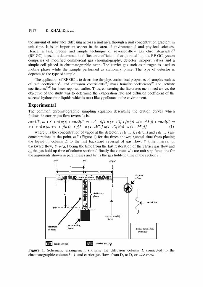
where c is the concentration of vapor at the detector, c1 (l’,…), c2(l’,...) and c3(l’,…) are concentrations at the point x=l’ (Figure 1) for the times shown; t0=total time from placing the liquid in column L to the last backward reversal of gas flow, t’=time interval of backward flow, τ= t-tM, t being the time from the last restoration of the carrier gas flow and tM the gas hold-up time of column section l; finally the various u’s are unit step functions for the arguments shown in parentheses and tM’ is the gas hold-up time in the section l’.

Figure 1. Schematic arrangement showing the diffusion column L connected to the chromatographic column l + l’ and carrier gas flows from D2 to D1 or vice versa.

Determination of Diffusion Coefficients 1918

For t’ smaller than both tM and tM’, each sample peak produced by two successive reversals is symmetrical and its maximum height h from the ending baseline is given by

),'(2~ tolch = (2)

Where c(l’,t0) is the vapor concentration at x=l’ and time t0. The concentration of the liquid can be found from the diffusion equation in the column L (c.f. Figure 1):

2z

czD

to

cz

∂

∂=

∂

∂ (3)

Where D is the diffusion coefficient of the vapor into the carrier gas. The solution of Eq. 3 is sought under the initial condition:

( ) 00. =zCz (4)

The boundary conditions at z = L ( ) ( )toctoLCz ,1, = (5)

( ) ( )tovczcDLzz ,'1/ =∂∂−

= (6)

Where v is the linear velocity of carrier gas, and the boundary condition at z= 0:

( ) ( )( )00/ 0 CzCkzcD czz −=∂∂−=

(7)

Where cz(0) is the actual concentration at the liquid interface at time t0, c0 the concentration of the vapor which would be in equilibrium with the bulk liquid phase, and kc a rate coefficient for the evaporation process. Eq. 7 expresses the equality of the diffusion flux for removal of vapors from the liquid surface and the evaporation flux due to departure of cz at the surface from the equilibrium value c0. When the Laplace transform of Eq. 3 is taken with respect to t0, a linear second-order differential equation results. It can be solved by using z Laplace transformation yielding

( ) ( ) 2sinh/0'cosh0 qqCzqzCzCz += (8)

Where

( ) 2/10/0 DPQ = (9)

and Cz(0) and Cz’(0) are the t0 Laplace transform of cz(0) and (∂cz/∂z)z=0 respectively. If one combines Eq. 8 with the t0 transforms of the boundary conditions (5), (6) and (7), the Laplace transform of c(l’,t0), denoted as C(l’,p0), is found:

( ) ( )( ) ( ) qLkcvqLDqvkcDqPckPlC c coshsinh//10/00,' +++= (10)

Inverse Laplace transformation of this equation to find c(l’,t0) is difficult. It can be achieved by using certain approximations which are different for small or for long times. In the first case qL is large, allowing both sinh qL and cosh qL to be approximated by exp (qL)/2. Then Eq.10 becomes

))/1)(/1/()exp(2)(/(),'( 00 DqvDqkqLDqpckpolC c ++−= (11)

Which, for high enough flow rates, further reduces to

))/(/))(exp(/2(),'( DkcqqqLvDkcCopolC +−= (12)

Taking now the inverse Laplace transform of this equation, one finds

[ ]

+

+= 2/1

0

)()(2

)/2()/(exp2

),'( toDt

LerfcDtokDkcL

v

coktolc c

c (13)


Finally, if one uses the relation erfc x ≅ exp (-x2)/ (τπ1/2), which is a good approximation for large values of x, Eq 13 becomes

12/1 ))2/12/)((4/exp()/(2

),'( 2/12 −+−= toktoLDtoLDv

coktolC c

c π (14)

Coming now to the other extreme, i.e. long time approximations, qL is small and the functions sinh qL and cosh qL of Eq. 10 can be expanded in Mc Laurin series, retaining only the first three terms in each of them. Then, from Eq. 10 one obtains

)))2/1)((()//((1)(/(),'( 220 LqkcvqLDqvkDqpcokpolC cc ++++= (15)

and by using Eq. 9 and rearranging this become

)/(/]2/)(1[

1),'(

LkvDvkDLkvpoLpo

cokpolC

ccc

c

+++++= (16)

For high enough flow rates kc can be neglected compared to v and 1 can be neglected in comparison with vL/2D. For instance, in a usual experimental situation it was calculated that vL/2D = 420. Adopting these approximations, Eq. 16 reduces, after some rearrangement, to:

220

/)(2

12),'(

LDLkpopovL

DckpolC

c

c

++= (17)

Finally, inverse Laplace transformation of this relation yields

{ }]/)(2exp[1)(

),'( 2LtoDkcL

DLkv

DcoktolC

c

c +−−

+= (18)

by considering maximum height h of the sample peaks in Eq. 2 and substituting in it the right hand side of Eq. 18 for c(l’,t0), one obtains h as an explicit function of time t0. In order to linearize the resulting relation, an infinity value h∞ for the peak height is required:

)](/[2 DLkvdcokh cc +=∞ (19)

Using this expression, we obtain tcLDkcLhhh ]/)(2[ln)ln( 2+−∞=−∞ (20)

Thus, the long enough times, for which Eq. 18 was derived, a plot of ln (h∞-h) vs. t0 is expected to be linear, and from the slope -2(kcL+D)/L2 a first approximate value of kc can be calculated from the known value of L and a literature or theoretically calculated value of D. This value of kc can now be used to plot small time data according to Eq. 14 which is substituted now for c(l’,t0) in Eq 2. After rearrangement logarithms are taken and there results

)/1)(4/(])/(/4ln[)]2/(ln[ 22/12/12/1

toDLDvcoktoktoLh cc −=+ π (21)

Now, a plot of the left hand side of this relation vs. 1/t0 will yield a first approximation of experimental value for D from the slope –L

2/4D of this new linear plot. This D value can be reused in the slope found from the plot of Eq. 20 to calculate a more accurate value for kc. In turn, the latter is utilized to report Eq. 21, so that a more accurate value for D is found. These iterations can be continued until no significant changes in the kc and D values results.

Chemicals n-Pentane, n-hexane, n-heptane and n-hexadecane from Merck-AR graded were used as evaporating liquids (stationary phase). Nitrogen of 99.99% purity from MOX (Malaysia) was used as the carrier gas (mobile phase).


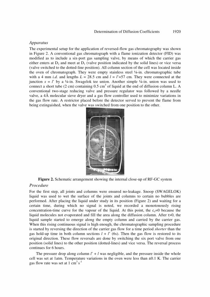
Apparatus The experimental setup for the application of reversed-flow gas chromatography was shown in Figure 2. A conventional gas chromatograph with a flame ionization detector (FID) was modified as to include a six-port gas sampling valve, by means of which the carrier gas either enters at D2 and meet at D1 (valve position indicated by the solid lines) or vice versa (valve switched to the dotted-line position). All column section of the cell was located inside the oven of chromatograph. They were empty stainless steel ¼-in. chromatographic tube with a 4 mm i.d. and lengths L = 28.5 cm and l = l’=57 cm. They were connected at the junction x = l’ by a ¼-in. Swagelok tee union. Another simple ¼-in. union was used to connect a short tube (2 cm) containing 0.5 cm3 of liquid at the end of diffusion column L. A conventional two-stage reducing valve and pressure regulator was followed by a needle valve, a 4Å molecular sieve dryer and a gas flow controller used to minimize variations in the gas flow rate. A restrictor placed before the detector served to prevent the flame from being extinguished, when the valve was switched from one position to the other.

Figure 2. Schematic arrangement showing the internal close-up of RF-GC system

Procedure

For the first step, all joints and columns were ensured no-leakage. Snoop (SWAGELOK) liquid was used to wet the surface of the joints and columns to certain no bubbles are performed. After placing the liquid under study in its position (Figure 2) and waiting for a certain time, during which no signal is noted, we recorded a monotonously rising concentration-time curve for the vapour of the liquid. At this point, the cz=0 because the liquid molecules not evaporated and fill the area along the diffusion column. After t>0, the liquid sample started to emerge along the empty column and carried by the carrier gas. When this rising continuous signal is high enough, the chromatographic sampling procedure is started by reversing the direction of the carrier gas flow for a time period shorter than the gas hold-up time in both column sections l + l’ (6s). Then the gas flow is restored to its original direction. These flow reversals are done by switching the six port valve from one position (solid lines) to the other position (dotted-lines) and vice versa. The reversal process continues for 6 hours.

The pressure drop along column l’ + l was negligible, and the pressure inside the whole cell was set at 1atm. Temperature variations in the oven were less than ±0.1 K. The carrier gas flow rate was set at 1 cm3 s-1

FID

sig

nal/

uV

t/min

Time / minutes

heig

ht


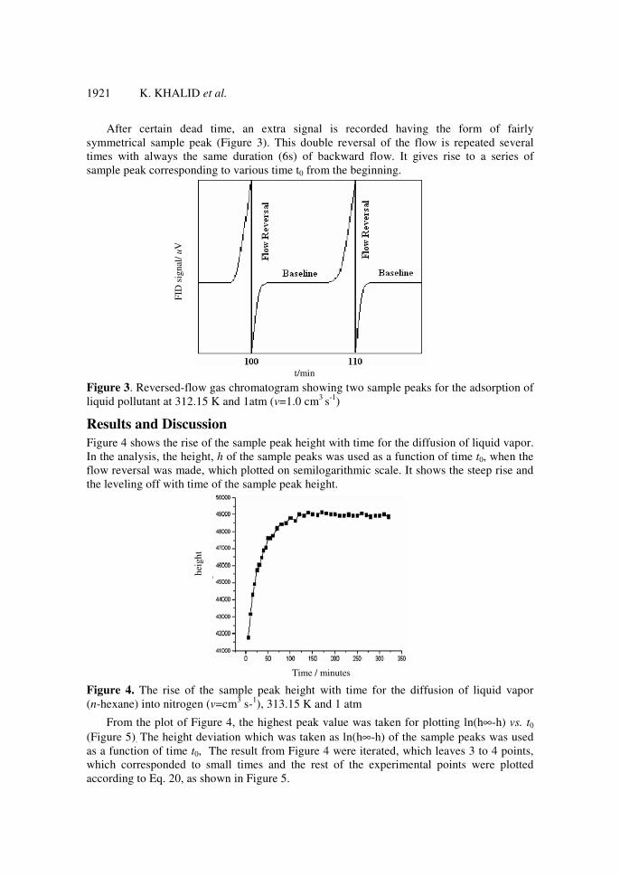
After certain dead time, an extra signal is recorded having the form of fairly symmetrical sample peak (Figure 3). This double reversal of the flow is repeated several times with always the same duration (6s) of backward flow. It gives rise to a series of sample peak corresponding to various time t0 from the beginning.

Figure 3. Reversed-flow gas chromatogram showing two sample peaks for the adsorption of liquid pollutant at 312.15 K and 1atm (v=1.0 cm3 s-1)

Results and Discussion

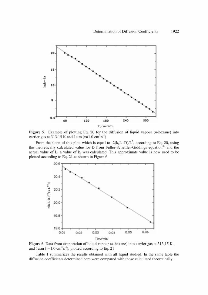
Figure 4 shows the rise of the sample peak height with time for the diffusion of liquid vapor. In the analysis, the height, h of the sample peaks was used as a function of time t0, when the flow reversal was made, which plotted on semilogarithmic scale. It shows the steep rise and the leveling off with time of the sample peak height.

Figure 4. The rise of the sample peak height with time for the diffusion of liquid vapor (n-hexane) into nitrogen (v=cm3 s-1), 313.15 K and 1 atm

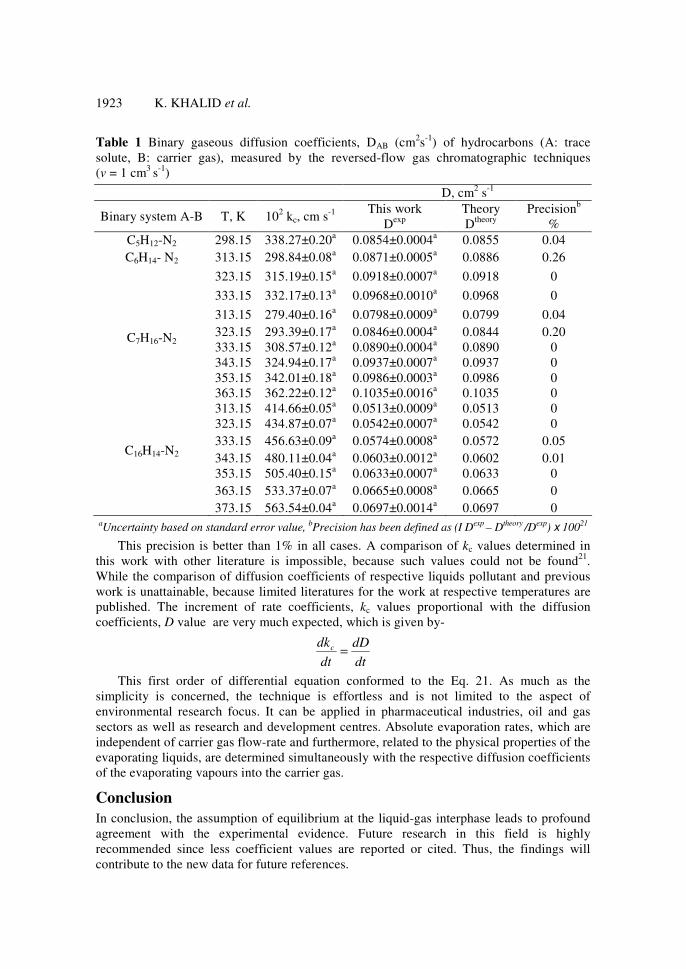
From the plot of Figure 4, the highest peak value was taken for plotting ln(h∞-h) vs. t0 (Figure 5). The height deviation which was taken as ln(h∞-h) of the sample peaks was used as a function of time t0, The result from Figure 4 were iterated, which leaves 3 to 4 points, which corresponded to small times and the rest of the experimental points were plotted according to Eq. 20, as shown in Figure 5.

ln(h

∞-h

)

To / minutes

Time/min-1

ln[h

(1/2

t 0)1/

2 +k c

t 01/

2 )]


Figure 5. Example of plotting Eq. 20 for the diffusion of liquid vapour (n-hexane) into carrier gas at 313.15 K and 1atm (v=1.0 cm3 s-1)

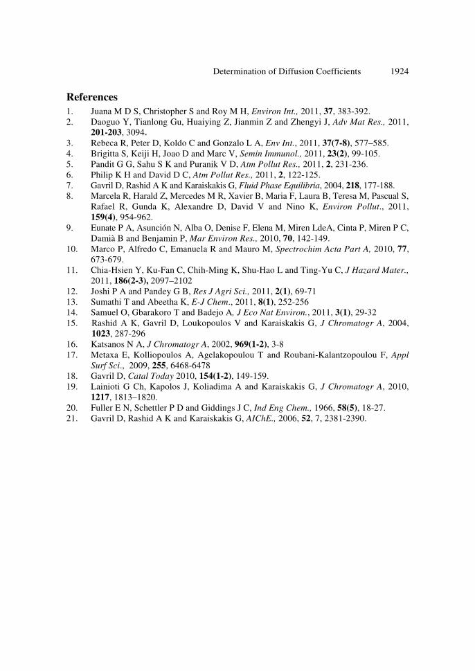
From the slope of this plot, which is equal to -2(koL+D)/L2, according to Eq. 20, using the theoretically calculated value for D from Fuller-Schettler-Giddings equation20 and the actual value of L, a value of kc was calculated. This approximate value is now used to be plotted according to Eq. 21 as shown in Figure 6.

Figure 6. Data from evaporation of liquid vapour (n-hexane) into carrier gas at 313.15 K and 1atm (v=1.0 cm3 s-1), plotted according to Eq. 21

Table 1 summarizes the results obtained with all liquid studied. In the same table the diffusion coefficients determined here were compared with those calculated theoretically.


Table 1 Binary gaseous diffusion coefficients, DAB (cm2s-1) of hydrocarbons (A: trace solute, B: carrier gas), measured by the reversed-flow gas chromatographic techniques (v = 1 cm3 s-1)

D, cm2 s-1

Binary system A-B T, K 102 kc, cm s-1 This work

Dexp Theory Dtheory

Precisionb %

C5H12-N2 298.15 338.27±0.20a 0.0854±0.0004a 0.0855 0.04 C6H14- N2 313.15 298.84±0.08a 0.0871±0.0005a 0.0886 0.26

323.15 315.19±0.15a 0.0918±0.0007a 0.0918 0

333.15 332.17±0.13a 0.0968±0.0010a 0.0968 0

313.15 279.40±0.16a 0.0798±0.0009a 0.0799 0.04 323.15 293.39±0.17a 0.0846±0.0004a 0.0844 0.20 333.15 308.57±0.12a 0.0890±0.0004a 0.0890 0 343.15 324.94±0.17a 0.0937±0.0007a 0.0937 0 353.15 342.01±0.18a 0.0986±0.0003a 0.0986 0

C7H16-N2

363.15 362.22±0.12a 0.1035±0.0016a 0.1035 0 313.15 414.66±0.05a 0.0513±0.0009a 0.0513 0 323.15 434.87±0.07a 0.0542±0.0007a 0.0542 0 333.15 456.63±0.09a 0.0574±0.0008a 0.0572 0.05 343.15 480.11±0.04a 0.0603±0.0012a 0.0602 0.01 353.15 505.40±0.15a 0.0633±0.0007a 0.0633 0

C16H14-N2

363.15 533.37±0.07a 0.0665±0.0008a 0.0665 0 373.15 563.54±0.04a 0.0697±0.0014a 0.0697 0

aUncertainty based on standard error value, bPrecision has been defined as (I Dexp – Dtheory /Dexp) x 10021

This precision is better than 1% in all cases. A comparison of kc values determined in this work with other literature is impossible, because such values could not be found21. While the comparison of diffusion coefficients of respective liquids pollutant and previous work is unattainable, because limited literatures for the work at respective temperatures are published. The increment of rate coefficients, kc values proportional with the diffusion coefficients, D value are very much expected, which is given by-

dt

dD

dt

dkc =

This first order of differential equation conformed to the Eq. 21. As much as the simplicity is concerned, the technique is effortless and is not limited to the aspect of environmental research focus. It can be applied in pharmaceutical industries, oil and gas sectors as well as research and development centres. Absolute evaporation rates, which are independent of carrier gas flow-rate and furthermore, related to the physical properties of the evaporating liquids, are determined simultaneously with the respective diffusion coefficients of the evaporating vapours into the carrier gas.

Conclusion

In conclusion, the assumption of equilibrium at the liquid-gas interphase leads to profound agreement with the experimental evidence. Future research in this field is highly recommended since less coefficient values are reported or cited. Thus, the findings will contribute to the new data for future references.


References

1. Juana M D S, Christopher S and Roy M H, Environ Int., 2011, 37, 383-392. 2. Daoguo Y, Tianlong Gu, Huaiying Z, Jianmin Z and Zhengyi J, Adv Mat Res., 2011,

201-203, 3094.

3. Rebeca R, Peter D, Koldo C and Gonzalo L A, Env Int., 2011, 37(7-8), 577–585. 4. Brigitta S, Keiji H, Joao D and Marc V, Semin Immunol., 2011, 23(2), 99-105. 5. Pandit G G, Sahu S K and Puranik V D, Atm Pollut Res., 2011, 2, 231-236. 6. Philip K H and David D C, Atm Pollut Res., 2011, 2, 122-125. 7. Gavril D, Rashid A K and Karaiskakis G, Fluid Phase Equilibria, 2004, 218, 177-188. 8. Marcela R, Harald Z, Mercedes M R, Xavier B, Maria F, Laura B, Teresa M, Pascual S,

Rafael R, Gunda K, Alexandre D, David V and Nino K, Environ Pollut., 2011, 159(4), 954-962.

9. Eunate P A, Asunción N, Alba O, Denise F, Elena M, Miren LdeA, Cinta P, Miren P C, Damià B and Benjamin P, Mar Environ Res., 2010, 70, 142-149.

10. Marco P, Alfredo C, Emanuela R and Mauro M, Spectrochim Acta Part A, 2010, 77, 673-679.

11. Chia-Hsien Y, Ku-Fan C, Chih-Ming K, Shu-Hao L and Ting-Yu C, J Hazard Mater., 2011, 186(2-3), 2097–2102

12. Joshi P A and Pandey G B, Res J Agri Sci., 2011, 2(1), 69-71 13. Sumathi T and Abeetha K, E-J Chem., 2011, 8(1), 252-256 14. Samuel O, Gbarakoro T and Badejo A, J Eco Nat Environ., 2011, 3(1), 29-32 15. Rashid A K, Gavril D, Loukopoulos V and Karaiskakis G, J Chromatogr A, 2004,

1023, 287-296 16. Katsanos N A, J Chromatogr A, 2002, 969(1-2), 3-8 17. Metaxa E, Kolliopoulos A, Agelakopoulou T and Roubani-Kalantzopoulou F, Appl

Surf Sci., 2009, 255, 6468-6478 18. Gavril D, Catal Today 2010, 154(1-2), 149-159. 19. Lainioti G Ch, Kapolos J, Koliadima A and Karaiskakis G, J Chromatogr A, 2010,

1217, 1813–1820. 20. Fuller E N, Schettler P D and Giddings J C, Ind Eng Chem., 1966, 58(5), 18-27. 21. Gavril D, Rashid A K and Karaiskakis G, AIChE., 2006, 52, 7, 2381-2390.

Submit your manuscripts athttp://www.hindawi.com

Hindawi Publishing Corporationhttp://www.hindawi.com Volume 2014

Inorganic ChemistryInternational Journal of

Hindawi Publishing Corporation http://www.hindawi.com Volume 2014

International Journal ofPhotoenergy


Carbohydrate Chemistry

International Journal of


Journal of

Chemistry


Advances in

Physical Chemistry

Hindawi Publishing Corporationhttp://www.hindawi.com

Analytical Methods in Chemistry

Journal of

Volume 2014

Bioinorganic Chemistry and ApplicationsHindawi Publishing Corporationhttp://www.hindawi.com Volume 2014

SpectroscopyInternational Journal of


The Scientific World JournalHindawi Publishing Corporation http://www.hindawi.com Volume 2014

Medicinal ChemistryInternational Journal of


Chromatography Research International


Applied ChemistryJournal of



Theoretical ChemistryJournal of


Journal of

Spectroscopy

Analytical ChemistryInternational Journal of


Journal of


Quantum Chemistry


Organic Chemistry International


CatalystsJournal of

ElectrochemistryInternational Journal of

Hindawi Publishing Corporation http://www.hindawi.com Volume 2014

Documents

Determination of Diffusion Coefficients of Selected Long ...downloads.hindawi.com/journals/jchem/2011/618308.pdf · Determination of Diffusion Coefficients 1918 For t’ smaller than