0

Treball realitzat per:

Javier Martín Sánchez

Dirigit per:

Tutor: Maribel Ortego

Tutor extern: Zongzhi Li

Màster en:

Enginyeria de Camins, Canals i Ports

Barcelona, Setembre 2017

Secció de Matemàtiques i Estadística

Departament d’Enginyeria Civil i Ambiental

TR

EBA

LL F

INA

L D

E M

ÀST

ER

Determination of Chicago Transit

Authority park-and-ride price

elasticities: spatial analysis and

socioeconomic patterns.

1

To my parents,

who gave me the opportunity

to develop this thesis in the United States.

1

ABSTRACT

People make decisions on how to spend scarce money and time on transport, reflecting in this

way not only their mobility needs but also their options and preferences. On the other hand,

government and operators seek users to adopt travel patterns which have a positive impact on

transportation systems and the environment through strategic investments and policies. Park-

and-ride are facilities that promote the use of rail transit, encouraging a transfer of commuters

from car to public transport. The aim of this thesis is to investigate the effect of increasing

parking charges at park-and-ride facilities on park-and-ride users and the impact on other

complementary transportation modes for the Chicago Area according to the spatial

configuration of the city. To address this objective, STOPS software, released by the Federal

Transit Administration of US will be used as a tool for travel demand forecasting. It will be

performed a pricing sensibility analysis to evaluate price sensitivity on travel demand. This

study provides a new insight in park-and-ride price elasticities for big cities that contributes

to a literature of little extend in this field. In particular for the Chicago metropolitan area, this

thesis provides a new assessment tool to improve park-and-ride management in the region

and operator’s performance towards a more sustainable and transit-oriented city.

Key words: park-and-ride, urban planning, price elasticity, spatial analysis

2

RESUM

El temps i els diners emprats en el transport influeixen en les decisions dels usuaris,

determinant així, no només les seves necessitats de mobilitat sinó també les diferents

possibles opcions i preferències. Per altre banda, l’administració i els operadors del transport

apliquen estratègies i polítiques que influencien als usuaris a optar cap a models de transport

més sostenibles i beneficiosos pel sistema. Els Park-and-ride es tracten de facilitats que

promouen l’ús de la xarxa de trens o busos, motivant als usuaris a passar de l’ús del cotxe al

transport públic. L’objectiu d’aquest treball és investigar l’efecte de l’increment del preu en

les tarifes d’aquests serveis de pàrquing i l’impacte sobre els usuaris que utilitzen aquests

serveis i també l’impacte sobre altres modes de transport complementaris a la ciutat de

Chicago, en relació a la configuració espacial de la ciutat. Per fer aquest estudi s’ha utilitzat

un software anomenat STOPS, producte de la Federal Transit Administration d’Estats Units.

S’ha realitzat un anàlisis de sensibilitat de demanda en relació als preus per avaluar la

sensibilitat del usuaris a aquests canvis. Aquest estudi és una nova aportació a la literatura

referida a l’elasticitat de preus en aquest camp. A més, per l’àrea metropolitana de Chicago,

aquest projecte serveix com una eina per la presa de decisions a l’hora de gestionar aquestes

infraestructures i millorar la eficiència de l’operadora per avançar cap un model de ciutat més

sostenible, enfocat a l’ús del transport públic.

Paraules clau: park-and-ride, planificació urbana, elasticitat de preus, anàlisis espacial.

3

ACKNOWLEDGMENTS

I would like to thank the following companies for their assistance with the collection of the

data used for the research:

- Regional Transit Administration of Chicago (RTA)

- Chicago Transit Authority (CTA)

4

INDEX

ABSTRACT

ACKNOWLEDGMENTS

1. INTRODUCTION AND OBJECTIVES. .......................................................................... 9

1.1 Motivation ..................................................................................................................... 9

1.2 Objectives .................................................................................................................... 11

1.3 Literature review ......................................................................................................... 11

2. STOPS MODELS FOR TRAVEL DEMAND FORECAST ......................................... 15

2.1 Introduction ................................................................................................................. 15

2.2 General overview of STOPS FTA............................................................................... 17

2.3 Stops components ........................................................................................................ 19

2.3.1 Model structure ................................................................................................... 19

2.3.2 Inputs ................................................................................................................... 21

2.3.3 STOPS models ..................................................................................................... 30

2.3.4 Outputs ................................................................................................................ 43

2.4 Comparison between software and the 4 UTPP .......................................................... 44

3. DETERMINATION OF CTA PARK-AND-RIDE PRICE ELASTICTIES ............... 47

3.1 Introduction ................................................................................................................. 47

3.2 Price elasticity theory and calculation ......................................................................... 49

3.3 Description of the inputs ............................................................................................. 53

3.3.1 Regional Transportation Authority’s regionally calibrated STOPS inputs ........ 53

3.3.2 Park-and-ride cost calibration and validation .................................................... 62

3.4 Results for Park-and-Ride elasticities ......................................................................... 68

3.4.1 Direct elasticities ................................................................................................. 69

3.4.2 Cross-elasticities ................................................................................................. 72

3.5 Spatial analysis ............................................................................................................ 75

3.5.1 Land use and socioeconomic variables ............................................................... 75

3.5.2 Spatial analysis ................................................................................................... 77

4. SUMMARY AND CONCLUSION. ................................................................................. 85

4.1 Summary ..................................................................................................................... 85

4.2 Findings ....................................................................................................................... 86

4.3 Future lines of research ............................................................................................... 88

REFERENCES

5

LIST OF FIGURES

FIGURE 2.1 STOPS general flow-chart process 20

FIGURE 2.2 Collection and processing of CTPP 2000 23

FIGURE 2.3 File merging to a unique defined geographic unit in STOPS 29

FIGURE 2.4 Representation of the elements of the system. 32

FIGURE 2.5 Step 2 of schedule-based path algorithm 34

FIGURE 2.6 Step 3 and 4 of schedule-based path algorithm 35

FIGURE 2.7 STOPS adaptation process. 36

FIGURE 2.8 Model decay factor for HBO trips. 38

FIGURE 2.9 Growth factoring flow chart 39

FIGURE 2.10 Origin-destination matrix rows and columns equilibrium. 39

FIGURE 2.11 Mode choice model for STOPS 41

FIGURE 2.12 STOPS nested structure of alternatives. 42

FIGURE 3.1 Graphic representation of elastic and inelastic elasticity 50

FIGURE 3.2 CTA rail and bus network 57

FIGURE 3.3 Metra rail network 58

FIGURE 3.4 Main road network in the Chicago Area 60

FIGURE 3.5 District definition for STOPS simulation and calibration 61

FIGURE 3.6 Predicted vs. actual park-and-ride cost in time units. 65

FIGURE 3.7 Kernel Density Estimation for CTA park-and-ride direct price

elasticities.

70

FIGURE 3.8 KDE for Greater Vancouver Region (GVR) park-and-ride

direct price elasticities. Khander Nurul Habib, Mohamed S.

Mahmoud and Jesse Coleman (2014)

71

FIGURE 3.9 Spatial analysis for direct elasticities on CTA park-and-ride

facilities

79

FIGURE 3.10 Spatial analysis for cross elasticities on CTA park-and-ride

facilities

82

FIGURE 3.11 Spatial analysis for ∆VMT in the area of influence of CTA

park-and-ride facilities

83

6

LIST OF TABLES

TABLE 2.1 CTPP parts and universe. 26

TABLE 2.2 GTFS required files for STOPS simulation 27

TABLE 2.3 GTFS optional files 28

TABLE 2.4 Combination of Scenarios, time-of-day and modes for GTFS

Path

33

TABLE 2.5 Cross-classified trip rates by auto ownership 37

TABLE 2.6 Cross-classified trip rates by auto ownership for HBO and

NHB.

38

TABLE 2.7 Comparison between STOPS model and conventional 4-step

forecasting model

45

TABLE 3.1 CTA weekday Park-and-Ride users. Peter J. Foote. Trip

purpose

52

TABLE 3.2 CTA Park-and-ride location and characteristics. 62

TABLE 3.3 CTA Park-and-ride time penalty and variables affecting user’s

decision.

64

TABLE 3.4 Constants for existing RTA calibration model. 64

TABLE 3.5 Predicted time cost penalization for the 17 CTA Park-and-ride

before calibration and validation.

66

TABLE 3.6 Validation. Comparison of predicted and actual weekday park-

and-ride occupancy.

67

TABLE 3.7 Direct elasticity for CTA park-and-ride facilities. 69

TABLE 3.8 Cross elasticities for Bus and Rail combination. 72

TABLE 3.9 Incremental vehicle-mile traveled by district for 5% and 10%

scenario.

74

TABLE 3.10 Reference parking price elasticities for a car-oriented city.

Todd Litman, Victoria Transport Policy Institute

75

TABLE 3.11 Various land use and socioeconomic variables affecting travel

behavior.

76

7

C

HA

PTE

R 1

8

INTRODUCTION AND OBJECTIVES

CH

AP

TER

1

9

1. INTRODUCTION AND OBJECTIVES.

1.1 Motivation

Since the beginning of civilization, the viability and economic success of communities

have been greatly determined by the efficiency of their transportation infrastructures. The

need for efficient transportation and land-use systems has never been more critical than

it is today. There are serious concerns in many areas about the high levels of traffic

congestion, mobile-source emissions, the sustainability of our growth patterns and travel,

and the related adverse impacts on regional and national productivity (Chandra R. Bhat,

2000).

To improve the efficiency of transportation systems, engineers are responsible to take

accurate planning decisions according to existing and future scenarios through forecast

models that evaluate the response of transportation demands. The limitations on financial

resources and constraints on environmental impacts in transportation investments have

added the need for a systematic evaluation of alternative plans associated with

transportation infrastructure provision.

In particular for big cities, where there is a certain viability for public transportation due

to its economies of scale, many alternative strategies have been implemented to increase

benefits in transportation systems with a reduced financial cost but with a considerable

impact in travel patterns. This is called Transit-Oriented Development (TOD). It consists

in a set of strategies that aim to integrate mobility and urban development in order to

decrease the need for long-distance traveling and improve the accessibility to cities. The

success of TOD is not only guaranteed by availability of public transportation systems.

Pedestrian and cycling mobility, as well as managing the use of parking, are the key

elements of it that allows to discourage the use of automobiles and encourage public

transport.

Park-and-ride facilities are part of this group of strategies associated to Transit-Oriented

Development of cities. They consists in parking lots at bus or rail stops that allow travelers

to transfer from automobile to transit. On the one hand, they can increase the effectiveness

of transit systems and help reduce the need for parking in the Central Business District

(CBD), where the space is scarce and valuable. Park-and-ride lots thus promote a more

10

efficient use of land in the region. On the other hand they provide storage for vehicles

until transit-oriented development around the station could accomplish the same task.

However, locating and managing commuter parking facilities in order to have a positive

impact in the system is a complex task. The amount of parking supplied influences the

demand for parking, and it is difficult to determine the optimal parking supply without

consideration of the cost and benefits providing the supply. Then, investigation in the

relation between park-and-ride pricing and demand response is crucial for a better

performance and management of the facilities.

In North America, extensive park-and-ride facilities have been installed in a number of

light and heavy urban rail systems. Experience in practices indicates that although park-

and-ride option is very attractive to commuters, do not always result in traffic congestion

reduction, due to rising car ownership and use and the phenomenon of generated traffic.

Special analysis has to be performed between user’s characteristics, city configurations

and park-and-ride facilities such that benefits for both operator and society are

maximized.

Chicago is the third-largest city in the United States and the major transportation hub.

Chicago Transit Authority is the main transit operator in the city and serves their citizens

with the second largest public transportation system in country covering the City of

Chicago and 40 surrounding suburbs. An extensive park-and-ride network is associated

to the CTA rail line. In total 17 facilities are spread across the city to offer coverage to

commuters who live in the metropolitan area.

User’s responsiveness to park-and-ride charges associated to CTA rail line has never been

determined before. It exists the need to make research on park-and-ride price sensitivity

in relation to demand. Price elasticity is the best indicator that explains this relation.

Information about park-and-ride elasticities for the Chicago Area is of high utility for the

operator to improve their management by changing pricing policies according to user’s

sensibilities and choices.

11

1.2 Objectives

The main objective of this thesis is focused on providing an assessment tool for park-and-

ride management in the city of Chicago to improve the performance of both the facilities

and the transportation networks towards a more sustainable and transit-oriented city.

In particular, the following singular goals will be achieved in this thesis.

1) Describe in detail the models used by a new software released by the Federal

Transit Administration of the United States to perform travel demand forecasting.

STOPS software will be used as a tool to evaluate travel demand in the Chicago

Area for the year 2015. Description of the models have to be taken into account

when analyzing results.

2) Implement the 17 park-and-ride facilities to the network system as an input for

STOPS simulation based on real data for 2015.

3) Evaluate the demand at the transportation system for different park-and-ride

pricing scenarios.

4) Determine for the park-and-ride network the direct and cross elasticities in

relation to travel mode alternatives.

5) Justify the price sensitivity trends according to spatial characteristics in the

metropolitan area of Chicago. For this part GIS will be used to facilitate the

manipulation of spatial information in an intuitive manner.

As commented above, the evaluation of price sensitivity is performed for 2015. This is

the last year from which all data needed for the analysis is available. Moreover, transport

price elasticities do not change from year to year. They are considered as constants

although variations can be produced from place to place and according relevant

modifications in the systems. For those reasons, performing a study for 2015 will anyway

contribute to explain the current paradigm for Chicago transportation network.

1.3 Literature review

In this section it is presented a summary of the state of art of contributions of previous

studies with regard transportation price elasticities and in particular parking price

elasticities.

12

In recent years there has been increasing interest in transportation demand management,

including pricing reforms, to achieve planning objectives such as congestion, accidents

and pollution reduction. A considerable body of research has analyzed how transport price

changes affect transport activity, including changes in fuel prices, road tolls, parking fees,

fares and transport service quality. Although these impacts vary widely, it possible to

identify certain patterns which allow these relationships to be modeled.

Some of the most relevant studies that have contributed to the determination of

transportation elasticities are TRACE 1999, Pratt 2004, Dargay and Hanly 2004, Warman

and Shires 2011 and Dahl 2012. They have measured various types of transport, prices,

users, travel conditions, and used various analysis methods. Some, simply evaluates the

changes in a single variables, but last studies released are using more complex evaluation

techniques, considering a variety of variables and statistical analysis. These models have

helped answer questions concerning the potential role that transit play in addressing

strategic transportation objectives such as congestion and emission reductions.

There exist several studies about parking price sensitivity, although they are more reduced

compared to other type of elasticties. Elasticities according to increase parking charges

are estimated in relation to various variables.

Kuzmyak, Weinberger and Levison (2003), performed a study which related parking

supply and travel demand, taking into account that reduced supply increases rates.

Washbrook, Haider and Jaccard (2006) contributed with a publication on the relations

between parking pricing and average car occupancy rates for the Vancouver Area. Frank,

et. al (2011) found the impact between parking rates change and emissions produced by

auto travelers who are affected by this type of policy. Barla, et. al (2012) measured the

marginal repercussion in users travel time of parking increased rates.

Other literature about parking price sensitivity is focused on auto users and transit riders,

reflecting the change of demand in this type of facilities and in transportation systems

through price elasticities. These references are of special interest for this thesis.

Harvey (1994) investigated on airport parking price sensitivity of users, obtaining a range

of elasticities from -0.1 for less than a day and -2.0 for greater than 8 days. Hensher and

King (2001) performed a study about parking facilities located in the CBD of Sidney, and

estimated the impact on users shifting to transit or moving to other facilities external to

13

downtown area. TRACE (1999) consists on one of the most complete publications about

transportation price elasticities. They provide detailed estimates of elasticities of various

type (car-trip, car-kilometers, transit travel, and slow modes.) with respect to parking

pricing.

Habib, Mahmoud and Coleman (2016) represents one of the latest studies about parking

price sensitivity, focused on park-and-ride facilities in the Greater Vancouver Region.

The research develops a Stated Performance Survey in the 14 busiest park-and-ride

facilities used to calibrate a mode choice model to estimate the impact in all-way transit

and auto travel by calculation direct and cross elasticties.

Many literature also refers to the transferability of the price elasticities through space and

time. Many of the studies summarized in this chapter are many years or decades old but

elasticties through time can be still valid, always applying criteria and evaluating current

conditions. Certainly, when using elasticities in a particular situation, it is important to

take into account those factors that have evolved after time. All the studies are performed

for big city areas, but it has to be considered differences between country, regions and

between cities. This is why the following study about price elasticities at the CTA park-

and-ride facilities will be compared to values obtained in other literature, but always

analyzing them in the context of the metropolitan area of Chicago.

14

CH

AP

TER

2

STOPS MODELS FOR TRAVEL DEMAND

FORECAST

15

2. STOPS MODELS FOR TRAVEL DEMAND

FORECAST

2.1 Introduction

Travel demand modeling is the process of estimating the number of people or vehicles

that will use a specific transportation facility in the future. It consists in an essential part

of transportation planning for investments in transit or highway systems. The goal is to

perform an analysis of the travel demand markets to assist decision makers to justify the

viability of a specific alternative in a project and provide the necessary information to

develop a future revenue projection. Among the main application are included the

development of overall transportation policies, planning studies and engineering design

of specific projects.

To do this, it is commonly used a travel demand forecasting model - a computer model

used to estimate travel behavior and travel demand for a specific future time frame, based

on a number of assumptions. It has to be taken into account that travel demand forecasting

might not result in a perfect number because of user-land-system complexity. The

transportation analysis must seek logical, sensible and reflective resulting scenarios that

can be defensible according to reality.

The conventional travel demand model is a four-step process. The unit of travel is the

trip, defined as a person o vehicle traveling from an origin to a destination with no

intermediate stops. Since people traveling for different reasons behave differently, four-

step models segment trips by trip purpose and time of the day. The usual number of trip

purposes are three: home-based work (HBW), home-based other (HBO) and non-home

based trips (NHB). These are distributed along the day but usually the analysis is

developed for peak and off-peak hours to show the difference between the changeable

demand and level of service of the systems from period to period.

The four steps in the conventional travel demand model are the trip generation, trip

distribution, mode choice and trip assignment.

Trip generation is the first step in the process. It estimates the number of trips of each

type that begin and end in each location based on the amount of activity in an analysis

area. This area is specified in each project. In most of the models, trips are aggregated to

16

a specific unit of geography, which are the traffic analysis zones (TAZ). TAZ boundaries

are usually major roadways, jurisdictional borders and geographic boundaries which are

defined to contain homogeneous land uses to the extent possible. Trip generation require

some explanatory variables (socioeconomic data such as population, households and

employment) for the modeled area. The result of this step is the total amount of trip

productions and trip attractions by traffic analysis zones and purpose that will interact

between each other to produce flows from zone to zone.

An important issue in this first step is data updating. Estimates of socioeconomic data by

TAZ are developed for a base year. This base year will be used for model calibration,

adjusting the main parameters to match the actual data. However, data must be updated

according to the year of forecast to estimate the future generation of each model area.

This is normally developed by growth factor models which extrapolate actual

socioeconomic and demographic data to the year of interest to represent the future

conditions.

Trip distribution determines the relation between trip productions and trip attraction

within traffic analysis zones. In other words, the process determines where the trips end

up once they leave their traffic analysis zones. This is done according to “attractiveness”

of a zone, based on the cost of travel between zones (actual monetary cost or time cost),

as well as the amount of trip-making activity in each area. Trip distribution produces a

matrix of origins and destinations between all the zones for each trip purpose. In the

process there are also models of external travel that estimates the trips that originate or

are destined outside the project’s geographic region. These models include elements of

trip generation and trip distribution, and so the outputs are trip tables representing external

travel.

The third step is the split of the trips distributed along the modeled area into travel modes.

This means determining the relative proportions of travelers that use each particular mode

of transportation. The mode definitions vary depending on the types of transportation

options offered in the model’s geographic region and the types of planning analyses

required. The most common split is between transit, auto and non-motorized modes of

transportation. Normally the transit modes are composed by access mode (walk and auto)

and service type (bus, heavy rail, light rail, commuter rail, etc…). Auto trips can also be

stratified by vehicle occupancy and non-motorized modes can include walking and

bicycling.

17

A mode choice model can have one of several different forms and specifications, ranging

from a diversion table based on local survey data and a reasonable annual growth factor

to a more complex nested logit structure. This last model account for a wider variety of

choices.

The outputs of the mode choice include person trip tables by mode and purpose and auto-

vehicle trip tables. The mode choice step is often done through multiple iterations of trip

distribution and assignment as part of feedback loop of the process.

The last step is the trip assignment. It determines the route or path that trips will take in

going from zone to zone and consists of separate highway and transit assignment

processes. The highway assignment processes converts origin-destination trips onto paths

along the highway network, resulting in traffic volumes absorbed by network links. Speed

and travel time estimates depending on the capacity of the links which reflect the road

congestion, are also outputs. On the other hand, the transit assignment consists on

determining the loading of individual transit routes and links resulting in line volumes

and stations boarding and alighting.

Once the model produces the transit and traffic volumes for each link and stations, results

must be calibrated to match actual ridership survey data. The process of calibration refers

to the usage of factors and parameters that help to fit the predicted data with the current

situation for a base scenario. It consists on a testing process, where the model is run

several times until it replicates the existing scenarios with an acceptable level of accuracy.

Once the model is calibrated to current conditions, it can be used to forecast future

scenarios.

2.2 General overview of STOPS FTA

In April 2013, the Federal Transit Administration developed a software to perform travel

demand forecasting following a simplified method to evaluate and rate proposed major

transit projects. The Simplified Trips-on-Project Software (STOPS) is a series of

programs designed to estimate transit project ridership using a streamlined set of

procedures that bypass the time-consuming process of developing and applying a regional

travel demand forecasting model. The main objectives of this software are the following:

● Estimate the predicted number of trips that would use a specific project for

existing and future scenarios.

18

● Quantify the trips-on-project that would be made by transit dependents, stratified

by access mode and service type.

● Predict the change in automobile vehicle-miles of travel (VMT) in the road

network based on the change in overall transit ridership between the existing and

the future forecast scenario.

The model structure of STOPS is quite similar, in concept, to the structure of a traditional

trip-based four step travel forecasting models, but what actually makes this software

much simpler compared to the conventional model are the following points:

● Origin-to-destination travel matrix construction are derived from Census data

rather than elaborate trip generation and trips distribution procedures (steps 1 and

2). Travel patterns and trip tables are directly extracted from journey to work flow

tabulations developed from Year 2000 Census Transportation Planning Package

(CTPP) that are updated to account for current and future year demographic

growth. This avoids the need to calibrate these tools to the degree of accuracy

required to estimate transit ridership.

● Representation of transit levels-of-service are derived from timetable information,

bypassing the need to develop detailed transit networks in the planning

environment when tabulating access, waiting and in-vehicle travel times from

zone-to-zone. Timetable information is already available at most agencies and is

much more accurate than the representations of travel time and frequencies

contained in typical planning networks. STOPS also incorporates highway

congestion using zone-to-zone roadway times and distances obtained from a

regional travel model maintained by the metropolitan planning organization

(MPO) of the area.

● STOPS is nationally calibrated and validated and it is locally auto-calibrated to

represent actual conditions, matching rider-survey datasets for specific regions or

even stations. The national calibration and validations used current ridership on

over 24 fixed-guide way systems in more than a dozen metropolitan areas in

United States. This means that the months and sometimes years, that are spent

developing and documenting effective forecasting tools can be avoided.

STOPS is complemented with the Geographic Information Systems (GIS) software to

update all the data contained in the geographic units from different sources (Census data,

MPO data and station locations). Any GIS software that can read ESRI Shape files can

19

be used. However, STOPS automates the linkage to two of the most common GIS

packages used in transportation analysis which are TransCAD and ArcMap.

2.3 Stops components

This part of the chapter comprises four different sections to describe the development of

the models that STOPS uses for the travel demand forecast. The first section is an

introduction to the general structure of stops to show an overview of the process in order

to know at each point which are the predecessor and postprocessor steps inside the whole

process. The following three corresponds to the development of the previous section

divided into:

● the inputs needed for running the software providing information about their

sources and content

● the specific models of calculation of STOPS, developing the formulas and

algorithms

● the outputs obtained at the end of the process and their practical utilization.

2.3.1 Model structure

Transport supply responds for the capacity of transportation infrastructures and modes,

generally over geographically defined transport systems and for a specific period of time.

It is expressed in terms of capacity, service and networks. Transport demand is translated

to transport needs, independently of the degree of coverage. It is expressed in terms of

number of people per unit of time and space.

Transportation supply and demand are directly dependent one to each other. For that

reason, the travel demand forecasting models are based on their constant interaction to

reach the equilibrium in the system. The supply over a geographical domain is defined by

the highway supply and the transit supply.

The general structure of STOPS can be cross-classified by inputs, models and outputs and

also by transit supply, highway supply and travel demand parallel tracks that are

interrelated along the process. The interaction between the different elements of the

process are shown in the flow chart of Figure 3.1.

20

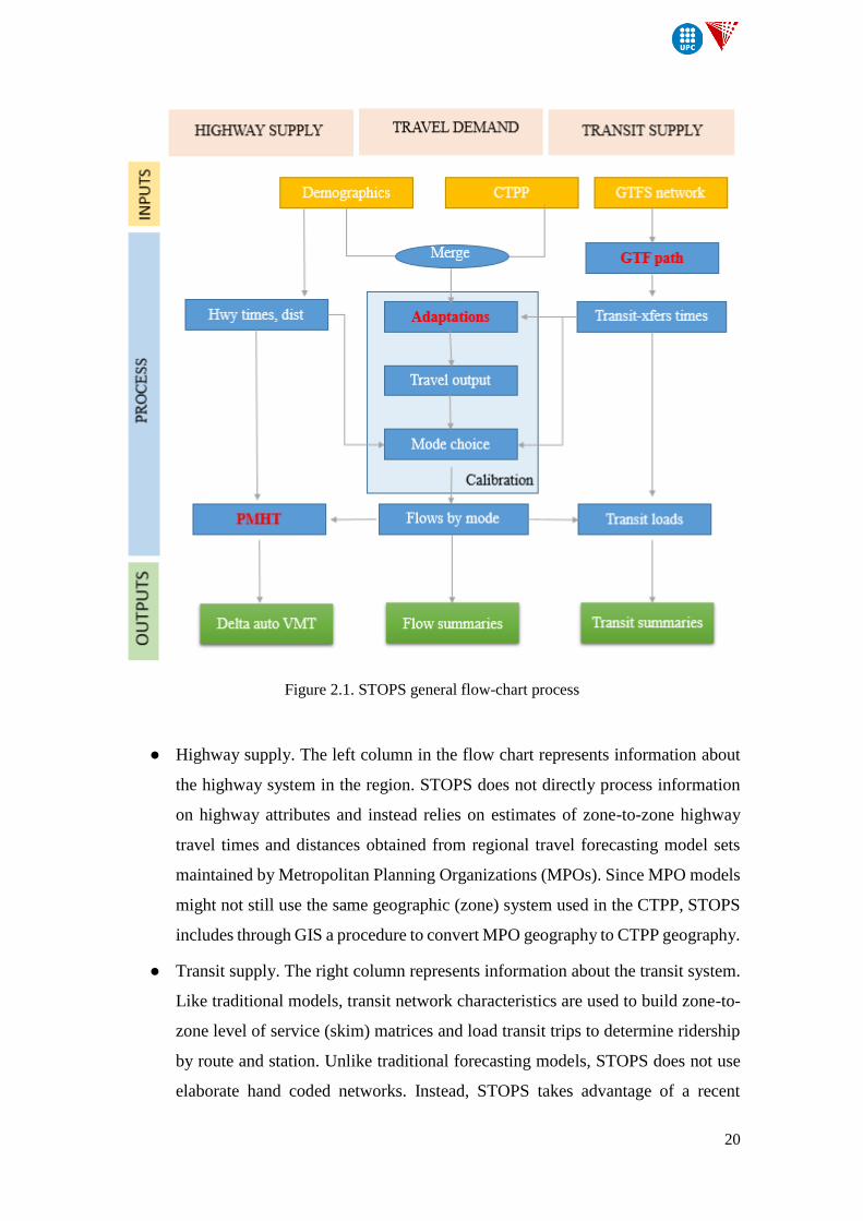
Figure 2.1. STOPS general flow-chart process

● Highway supply. The left column in the flow chart represents information about

the highway system in the region. STOPS does not directly process information

on highway attributes and instead relies on estimates of zone-to-zone highway

travel times and distances obtained from regional travel forecasting model sets

maintained by Metropolitan Planning Organizations (MPOs). Since MPO models

might not still use the same geographic (zone) system used in the CTPP, STOPS

includes through GIS a procedure to convert MPO geography to CTPP geography.

● Transit supply. The right column represents information about the transit system.

Like traditional models, transit network characteristics are used to build zone-to-

zone level of service (skim) matrices and load transit trips to determine ridership

by route and station. Unlike traditional forecasting models, STOPS does not use

elaborate hand coded networks. Instead, STOPS takes advantage of a recent

21

advance in on-line schedule data: the General Transit Feed Specification (GTFS).

This data format is a commonly-used format for organizing transit data so that on-

line mapping programs can help customers find the optimal paths (times, routes,

and stop locations) for their trips. STOPS includes a model known as GTFSPath

that generates the shortest path between every combination of regional origin and

destination. This path is used for estimating travel times (as an input to mode

choice) and for assigning transit trips (an output of mode choice) to routes and

stations.

● Travel Demand. The central column represents the demand side of STOPS.

STOPS uses Year 2000 CTPP Journey-to-Work data to estimate zone-to-zone

demand for travel (i.e., travel flows) as an input to the models that determine the

mode of travel. This data is adapted to represent current and future years by using

MPO demographic forecasts to account for zone-specific growth in population

and employment. A traditional nested logit mode choice model is used to

determine the proportion of trips utilizing transit stratified by access mode and

transit sub-mode. Results of mode choice are summarized in a series of district-

to-district flow tables.

From the previous flow chart, we find some steps that are exactly the same as the four-

step process modeling and some other which are special models developed by STOPS.

These are the program to prepare the skim matrices (GTFS path), the models for

adaptations of the input data for the conversion to updated trip flows, and the calculation

of the Person-miles hour traveled by auto to estimate the variation of highway flows.

Special consideration will be taken in these models in the following sections.

2.3.2 Inputs

Many data are required for model development, validation and application. Model

application data primarily include socioeconomic data and transportation networks. These

data form the foundation of the model for an area, and if they do not meet a basic level of

accuracy, the model may never obtain acceptable forecast travel results.

22

MPO data:

A metropolitan planning organization (MPO) is a federally mandated and federally

funded transportation policy-making organization in the United States that is made up of

representatives from local government and governmental transportation authorities. Their

function is to work in tandem with state and transit agencies, and perform a coordinating

role in the transportation planning process of a region.

STOPS uses data from the local Metropolitan Planning Organizations (MPO) contained

in ESRI shape files to describe the agency’s traffic analysis systems. The information

provided at the TAZ level comprises:

● Population and employment datasets

● Zone-to-zone automobile travel times and distances.

Population and employment data are available for year 2000, current and projected future-

year. The main use of this data is to update the socioeconomic information provided by

the Census of Transportation Planning Package 2000 to current and future conditions, so

that predictions about travel patterns can be extrapolated from the base year.

In fact, there exists many sources from which population and employment data can be

extracted but many of them fail to provide accurate numbers due to their collection

process. Especially employment data are difficult to track as they are more changeable

than households. Therefore, database for those variables in STOPS are obtained from

MPO’s as these organizations work locally on a region and offers a more complete and

detailed inventory than other national sources.

Zone to zone current year peak period automobile travel times and distances are obtained

from the regional travel demand forecasting model developed by MPO’s in their region.

These matrixes are constructed based on the minimum network distances between zones

and the speeds for peak and off-peak periods for each type of road (freeways, major

arterials and minor arterials). An iterative process is carried out in the region travel

demand model to reach equilibrium according to traveler’s choices and actual state of

congestion of the system. Apart from the data about the current year, it could be available

information about times and distances for an opening or forecast years (10 or 20 years

ahead).

23

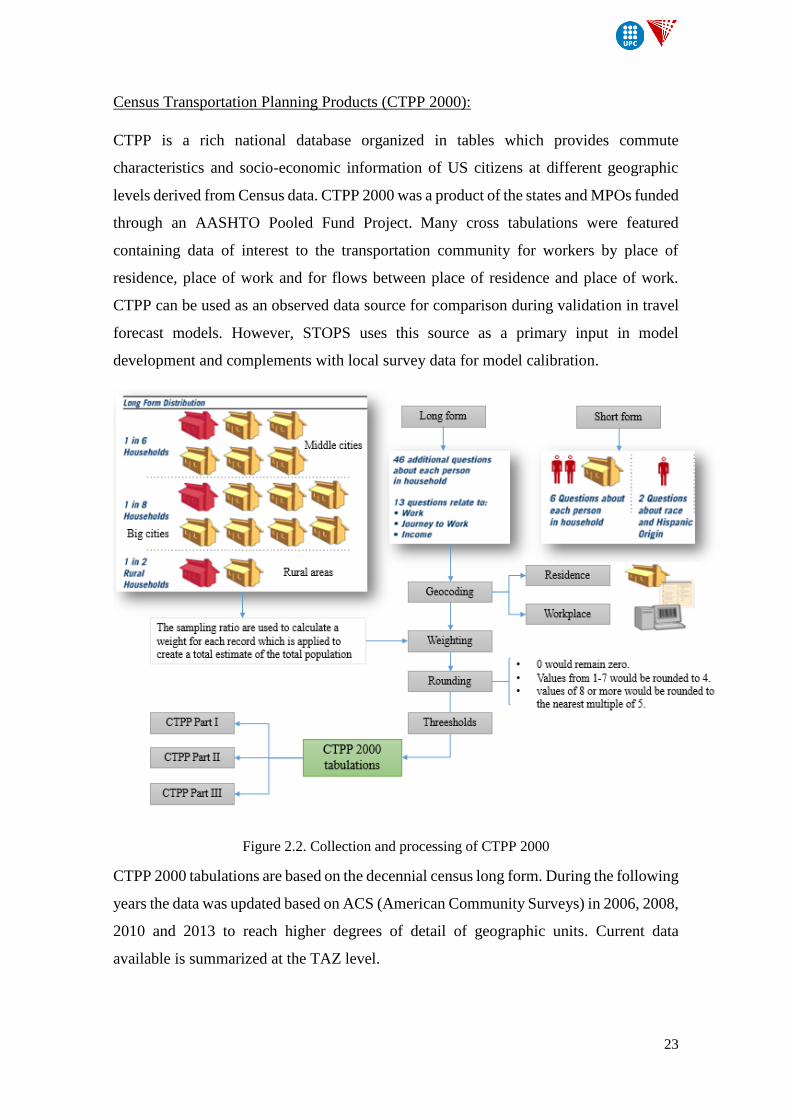
Census Transportation Planning Products (CTPP 2000):

CTPP is a rich national database organized in tables which provides commute

characteristics and socio-economic information of US citizens at different geographic

levels derived from Census data. CTPP 2000 was a product of the states and MPOs funded

through an AASHTO Pooled Fund Project. Many cross tabulations were featured

containing data of interest to the transportation community for workers by place of

residence, place of work and for flows between place of residence and place of work.

CTPP can be used as an observed data source for comparison during validation in travel

forecast models. However, STOPS uses this source as a primary input in model

development and complements with local survey data for model calibration.

Figure 2.2. Collection and processing of CTPP 2000

CTPP 2000 tabulations are based on the decennial census long form. During the following

years the data was updated based on ACS (American Community Surveys) in 2006, 2008,

2010 and 2013 to reach higher degrees of detail of geographic units. Current data

available is summarized at the TAZ level.

24

When the first data for CTPP was collected, all United States citizens were required to

complete the decennial census forms. Because it was mandatory to complete and because

of the intensive field work, the 2000 Census had a very high response rate. This means

that there were nearly 100 percent count of citizens by sex, age and race (Census Short

Form) and an average of 1 in 6 sample of wide variety of other person, household, worker,

and journey-to-work characteristics (Census Long Form). The ratio of samples of the

Long Form depended on the population density in the area, and could vary from one in

two to one to eight. The Long Form included the same questions as the Short form and

included additionally 46 more questions. Out of this 46 questions, 13 were related to

work, journey to work, vehicle availability and income.

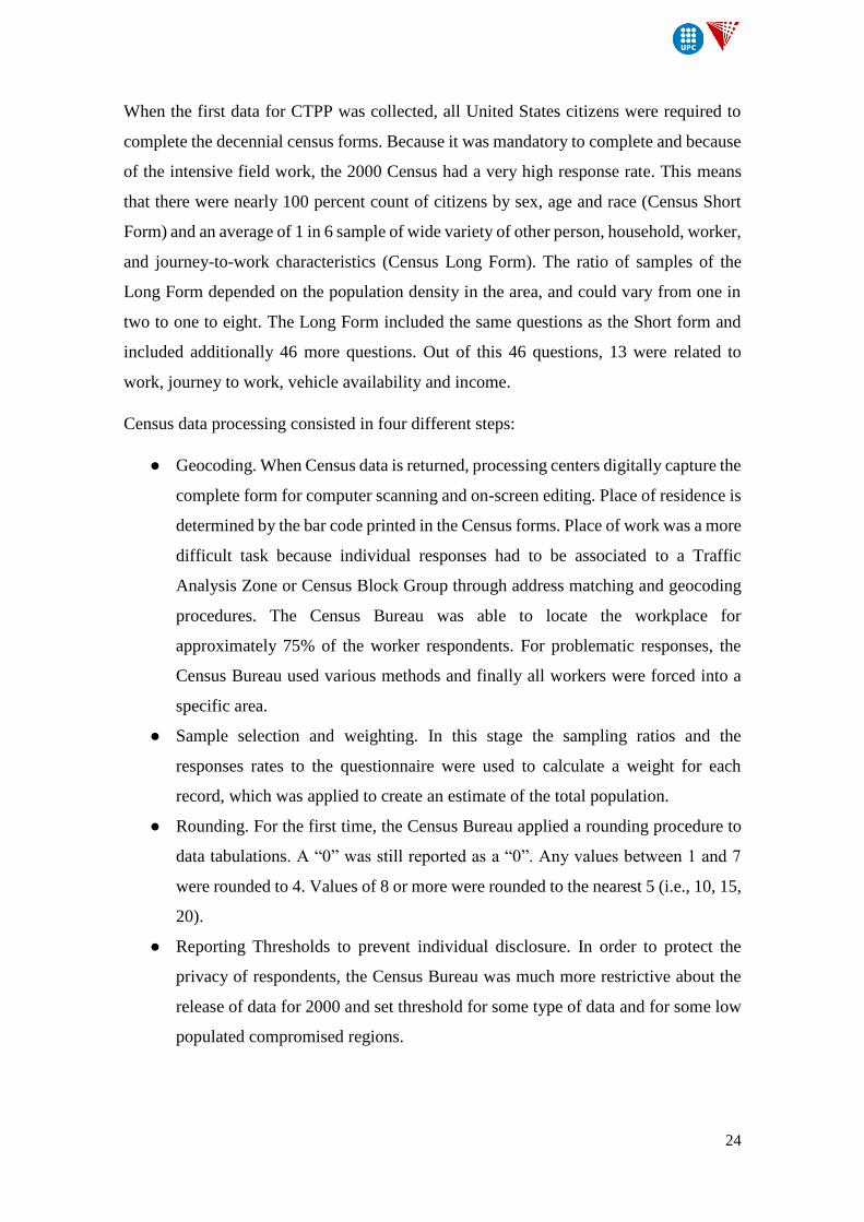
Census data processing consisted in four different steps:

● Geocoding. When Census data is returned, processing centers digitally capture the

complete form for computer scanning and on-screen editing. Place of residence is

determined by the bar code printed in the Census forms. Place of work was a more

difficult task because individual responses had to be associated to a Traffic

Analysis Zone or Census Block Group through address matching and geocoding

procedures. The Census Bureau was able to locate the workplace for

approximately 75% of the worker respondents. For problematic responses, the

Census Bureau used various methods and finally all workers were forced into a

specific area.

● Sample selection and weighting. In this stage the sampling ratios and the

responses rates to the questionnaire were used to calculate a weight for each

record, which was applied to create an estimate of the total population.

● Rounding. For the first time, the Census Bureau applied a rounding procedure to

data tabulations. A “0” was still reported as a “0”. Any values between 1 and 7

were rounded to 4. Values of 8 or more were rounded to the nearest 5 (i.e., 10, 15,

20).

● Reporting Thresholds to prevent individual disclosure. In order to protect the

privacy of respondents, the Census Bureau was much more restrictive about the

release of data for 2000 and set threshold for some type of data and for some low

populated compromised regions.

25

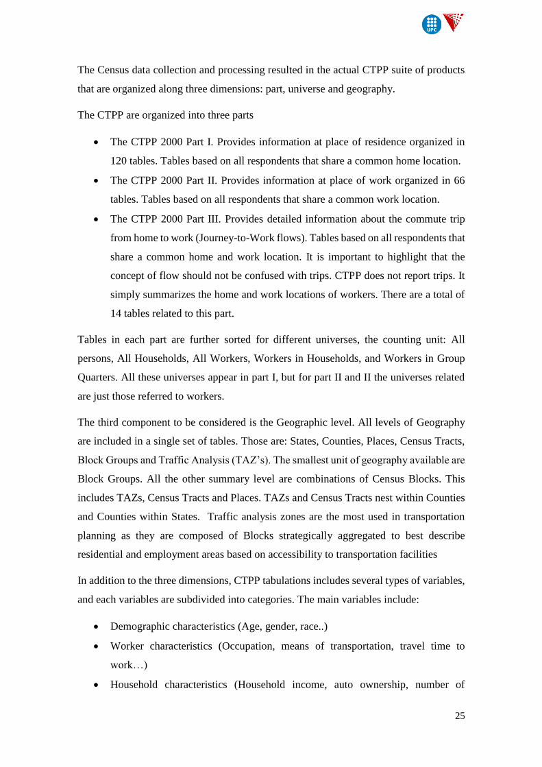
The Census data collection and processing resulted in the actual CTPP suite of products

that are organized along three dimensions: part, universe and geography.

The CTPP are organized into three parts

The CTPP 2000 Part I. Provides information at place of residence organized in

120 tables. Tables based on all respondents that share a common home location.

The CTPP 2000 Part II. Provides information at place of work organized in 66

tables. Tables based on all respondents that share a common work location.

The CTPP 2000 Part III. Provides detailed information about the commute trip

from home to work (Journey-to-Work flows). Tables based on all respondents that

share a common home and work location. It is important to highlight that the

concept of flow should not be confused with trips. CTPP does not report trips. It

simply summarizes the home and work locations of workers. There are a total of

14 tables related to this part.

Tables in each part are further sorted for different universes, the counting unit: All

persons, All Households, All Workers, Workers in Households, and Workers in Group

Quarters. All these universes appear in part I, but for part II and II the universes related

are just those referred to workers.

The third component to be considered is the Geographic level. All levels of Geography

are included in a single set of tables. Those are: States, Counties, Places, Census Tracts,

Block Groups and Traffic Analysis (TAZ’s). The smallest unit of geography available are

Block Groups. All the other summary level are combinations of Census Blocks. This

includes TAZs, Census Tracts and Places. TAZs and Census Tracts nest within Counties

and Counties within States. Traffic analysis zones are the most used in transportation

planning as they are composed of Blocks strategically aggregated to best describe

residential and employment areas based on accessibility to transportation facilities

In addition to the three dimensions, CTPP tabulations includes several types of variables,

and each variables are subdivided into categories. The main variables include:

Demographic characteristics (Age, gender, race..)

Worker characteristics (Occupation, means of transportation, travel time to

work…)

Household characteristics (Household income, auto ownership, number of

26

persons in the household…)

Housing unit characteristics (vacancy status, units in the structure…)

Categories from most of the variables are cross-tabulated with other categories to classify

data in a way that reflects key information to develop travel demand forecasting.

The content of Census Transportation Planning Products is very extent. STOPS is not

using all the tables corresponding to the three parts. From the 120 tables of Part I, STOPS

uses the first group of tables (1-29) of universe All Workers. From the 68 tables of Part

II, tables referred to Workers in Households from 30-48 are used as inputs. All the 14

tables in Part III are needed for the model application.

Part 1. At Residence (121 Tables)

Group 1: All Workers Tables 1-29

Group 2: Workers in Households Tables 30-48

Group 3: Persons Tables 49-61

Group 4: Households Tables 62-83

Group 5: Housing Units Tables 84-88

Group 6: Computed Tables Tables 89-121

Part 2: At Workplace (68 Tables)

Group 1: All workers Tables 1-29

Group 2: Workers in Households Tables 30-48

Group 3: Computed Tables Tables 49-68

Part 3: Worker Flows (14 tables)

Group 1: Small geography Tables 1-8

Group 2: Sm Geo Computed Tables 9-14

Table 2.1. CTPP 2000 table structure: parts and universe.

CTPP tables are in text format. To work correctly with STOPS, when uploading these

files as inputs, two more ESRI shape files are added, containing the description of the

boundaries of the census geography used in the remaining CTPP files corresponding the

states of the corridor being modeled.

27

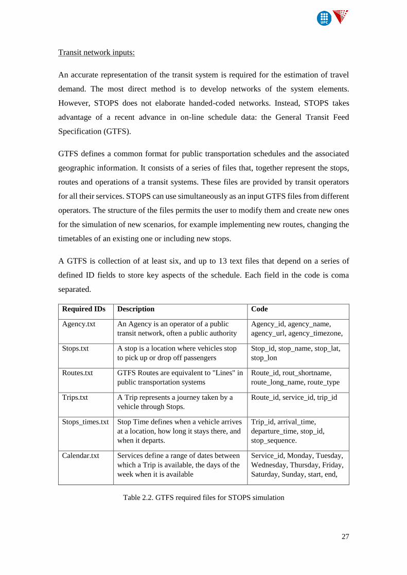
Transit network inputs:

An accurate representation of the transit system is required for the estimation of travel

demand. The most direct method is to develop networks of the system elements.

However, STOPS does not elaborate handed-coded networks. Instead, STOPS takes

advantage of a recent advance in on-line schedule data: the General Transit Feed

Specification (GTFS).

GTFS defines a common format for public transportation schedules and the associated

geographic information. It consists of a series of files that, together represent the stops,

routes and operations of a transit systems. These files are provided by transit operators

for all their services. STOPS can use simultaneously as an input GTFS files from different

operators. The structure of the files permits the user to modify them and create new ones

for the simulation of new scenarios, for example implementing new routes, changing the

timetables of an existing one or including new stops.

A GTFS is collection of at least six, and up to 13 text files that depend on a series of

defined ID fields to store key aspects of the schedule. Each field in the code is coma

separated.

Required IDs Description Code

Agency.txt An Agency is an operator of a public

transit network, often a public authority

Agency_id, agency_name,

agency_url, agency_timezone,

Stops.txt A stop is a location where vehicles stop

to pick up or drop off passengers

Stop_id, stop_name, stop_lat,

stop_lon

Routes.txt GTFS Routes are equivalent to "Lines" in

public transportation systems

Route_id, rout_shortname,

route_long_name, route_type

Trips.txt A Trip represents a journey taken by a

vehicle through Stops.

Route_id, service_id, trip_id

Stops_times.txt Stop Time defines when a vehicle arrives

at a location, how long it stays there, and

when it departs.

Trip_id, arrival_time,

departure_time, stop_id,

stop_sequence.

Calendar.txt Services define a range of dates between

which a Trip is available, the days of the

week when it is available

Service_id, Monday, Tuesday,

Wednesday, Thursday, Friday,

Saturday, Sunday, start, end,

Table 2.2. GTFS required files for STOPS simulation

28

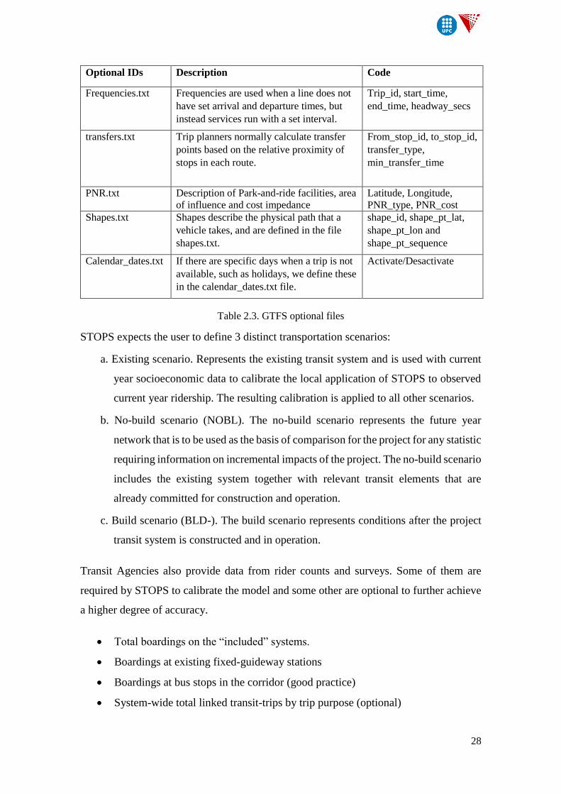
Optional IDs Description Code

Frequencies.txt Frequencies are used when a line does not

have set arrival and departure times, but

instead services run with a set interval.

Trip_id, start_time,

end_time, headway_secs

transfers.txt Trip planners normally calculate transfer

points based on the relative proximity of

stops in each route.

From_stop_id, to_stop_id,

transfer_type,

min_transfer_time

PNR.txt Description of Park-and-ride facilities, area

of influence and cost impedance

Latitude, Longitude,

PNR_type, PNR_cost

Shapes.txt Shapes describe the physical path that a

vehicle takes, and are defined in the file

shapes.txt.

shape_id, shape_pt_lat,

shape_pt_lon and

shape_pt_sequence

Calendar_dates.txt If there are specific days when a trip is not

available, such as holidays, we define these

in the calendar_dates.txt file.

Activate/Desactivate

Table 2.3. GTFS optional files

STOPS expects the user to define 3 distinct transportation scenarios:

a. Existing scenario. Represents the existing transit system and is used with current

year socioeconomic data to calibrate the local application of STOPS to observed

current year ridership. The resulting calibration is applied to all other scenarios.

b. No-build scenario (NOBL). The no-build scenario represents the future year

network that is to be used as the basis of comparison for the project for any statistic

requiring information on incremental impacts of the project. The no-build scenario

includes the existing system together with relevant transit elements that are

already committed for construction and operation.

c. Build scenario (BLD-). The build scenario represents conditions after the project

transit system is constructed and in operation.

Transit Agencies also provide data from rider counts and surveys. Some of them are

required by STOPS to calibrate the model and some other are optional to further achieve

a higher degree of accuracy.

Total boardings on the “included” systems.

Boardings at existing fixed-guideway stations

Boardings at bus stops in the corridor (good practice)

System-wide total linked transit-trips by trip purpose (optional)

29

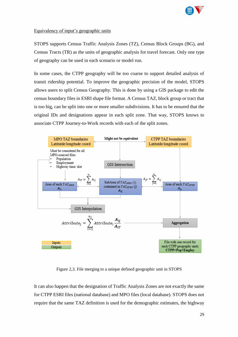
Equivalency of input’s geographic units

STOPS supports Census Traffic Analysis Zones (TZ), Census Block Groups (BG), and

Census Tracts (TR) as the units of geographic analysis for travel forecast. Only one type

of geography can be used in each scenario or model run.

In some cases, the CTPP geography will be too coarse to support detailed analysis of

transit ridership potential. To improve the geographic precision of the model, STOPS

allows users to split Census Geography. This is done by using a GIS package to edit the

census boundary files in ESRI shape file format. A Census TAZ, block group or tract that

is too big, can be split into one or more smaller subdivisions. It has to be ensured that the

original IDs and designations appear in each split zone. That way, STOPS knows to

associate CTPP Journey-to-Work records with each of the split zones.

Figure 2,3. File merging to a unique defined geographic unit in STOPS

It can also happen that the designation of Traffic Analysis Zones are not exactly the same

for CTPP ESRI files (national database) and MPO files (local database). STOPS does not

require that the same TAZ definition is used for the demographic estimates, the highway

30

travel impedances and the CTPP data. STOPS uses again internal GIS-like functions to

associate the data across the potentially different small-area definitions used in the various

data sources. The permanent TAZ definition will be the one defined by CTPP and the

final results is a file with one record containing CTPP data, population, employment and

other network characteristics.

2.3.3 STOPS models

In this part of the chapter it will be described the specific models of calculation of STOPS

based on the inputs previously described. The models will be grouped by the initial

categories presented in the flow chart in figure 3.1.: highway supply, transit supply and

travel demand. All the processes inside each category are also dependent of the other ones

as STOPS travel demand model does not follow a linear consecutive direction but consists

on the simultaneous calculations and adjustments at each step.

Highway supply.

Being STOPS a software for travel demand forecasting of transit projects, efforts are

focused on defining a precise transit service schedule to better determine the level of

services of the different systems. On the other hand, highway network has not a specific

development inside STOPS models. No physical elements representing roads and

connecting nodes are used to represent the highway supply. Instead, STOPS relays on the

data released by Metropolitan Planning Organizations about highway times and distances

between zones extracted from regional travel demand forecast.

These values are obtained for a base year and are also updated to the current year and

forecast year. The main problem about the inputs of time and distance is that the values

are static as they do not depend on the modifications of demand of the total system or

changes produced in the physical infrastructure supply during the years. This misleads

the fact that an increase of users in the highway system may lead to a decrease of speeds

and at the same time to an increase of the times from zone to zone.

Taking into account the previous point, STOPS defines a variable to evaluate the

utilization of the highway network. It is the estimation of automobile person miles of

travel that result from a scenario. It represents the total distance traveled by all the users

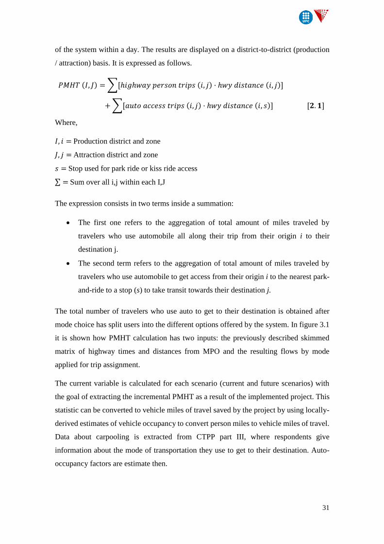
31

of the system within a day. The results are displayed on a district-to-district (production

/ attraction) basis. It is expressed as follows.

𝑃𝑀𝐻𝑇 (𝐼, 𝐽) = ∑[ℎ𝑖𝑔ℎ𝑤𝑎𝑦 𝑝𝑒𝑟𝑠𝑜𝑛 𝑡𝑟𝑖𝑝𝑠 (𝑖, 𝑗) · ℎ𝑤𝑦 𝑑𝑖𝑠𝑡𝑎𝑛𝑐𝑒 (𝑖, 𝑗)]

+ ∑[𝑎𝑢𝑡𝑜 𝑎𝑐𝑐𝑒𝑠𝑠 𝑡𝑟𝑖𝑝𝑠 (𝑖, 𝑗) · ℎ𝑤𝑦 𝑑𝑖𝑠𝑡𝑎𝑛𝑐𝑒 (𝑖, 𝑠)] [𝟐. 𝟏]

Where,

𝐼, 𝑖 = Production district and zone

𝐽, 𝑗 = Attraction district and zone

𝑠 = Stop used for park ride or kiss ride access

∑ = Sum over all i,j within each I,J

The expression consists in two terms inside a summation:

The first one refers to the aggregation of total amount of miles traveled by

travelers who use automobile all along their trip from their origin i to their

destination j.

The second term refers to the aggregation of total amount of miles traveled by

travelers who use automobile to get access from their origin i to the nearest park-

and-ride to a stop (s) to take transit towards their destination j.

The total number of travelers who use auto to get to their destination is obtained after

mode choice has split users into the different options offered by the system. In figure 3.1

it is shown how PMHT calculation has two inputs: the previously described skimmed

matrix of highway times and distances from MPO and the resulting flows by mode

applied for trip assignment.

The current variable is calculated for each scenario (current and future scenarios) with

the goal of extracting the incremental PMHT as a result of the implemented project. This

statistic can be converted to vehicle miles of travel saved by the project by using locally-

derived estimates of vehicle occupancy to convert person miles to vehicle miles of travel.

Data about carpooling is extracted from CTPP part III, where respondents give

information about the mode of transportation they use to get to their destination. Auto-

occupancy factors are estimate then.

32

Transit supply

Transit timetable data from local General Transit Feed Specification (GTFS) files are

used to develop zone-to-zone transit, access and waiting times. STOPS includes a

program known as GTFPath that generates the shortest path between every combination

of regional origin destination. This path is used for estimating travel times as an input for

mode choice and for assigning transit trips (an output of mode choice) to routes and

stations.

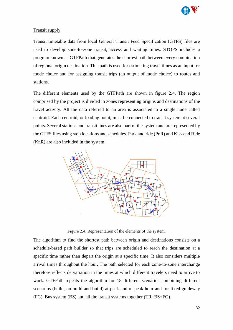
The different elements used by the GTFPath are shown in figure 2.4. The region

comprised by the project is divided in zones representing origins and destinations of the

travel activity. All the data referred to an area is associated to a single node called

centroid. Each centroid, or loading point, must be connected to transit system at several

points. Several stations and transit lines are also part of the system and are represented by

the GTFS files using stop locations and schedules. Park and ride (PnR) and Kiss and Ride

(KnR) are also included in the system.

Figure 2.4. Representation of the elements of the system.

The algorithm to find the shortest path between origin and destinations consists on a

schedule-based path builder so that trips are scheduled to reach the destination at a

specific time rather than depart the origin at a specific time. It also considers multiple

arrival times throughout the hour. The path selected for each zone-to-zone interchange

therefore reflects de variation in the times at which different travelers need to arrive to

work. GTFPath repeats the algorithm for 18 different scenarios combining different

scenarios (build, no-build and build) at peak and of-peak hour and for fixed guideway

(FG), Bus system (BS) and all the transit systems together (TR=BS+FG).

33

Scenario Time-of-day Mode

- Existing

- No-build

- Build

- Peak (8-9 am) 6

posible arrival times

- Off-peak (1-2 pm) 6

posible arrival times

- Fixed guideway (FG)

- Bus (BS)

- All Transit

(TR=BS+FG)

Table 2.4. Combination of Scenarios, time-of-day and modes for GTFS path

The algorithm used for calculating the shortest path between two zones is a scheduled-

based path builder with a fixed arrival time at the destination. The time-dependent

quickest path is developed from Dijkstra’s algorithm, and it uses travel time between

notes as the path cost (as based on the timetable) to make a selection of optimal nodes

and then apply a branch algorithm which finds the real shortest path between origins and

destinations from a reduced set of nodes. The algorithm is defined in 4 steps:

1) Time cost weighting definition. STOPS defines a generalized weighting function (in

weighted minutes) for selection of best path:

𝑊𝑖𝑗 = 𝛽 · 𝐴𝑇 + 1.0 · 𝑊𝑇 + 1.0 · 𝐼𝑉𝑇𝑇 + 5 [𝑚𝑖𝑛] [𝟐. 𝟐]

𝛽 = {1.1 𝑊𝑎𝑙𝑘𝑖𝑛𝑔

1.5 𝐾𝑁𝑅 𝑜𝑟 𝑃𝑁𝑅

Where,

Access time AT. Walking time is calculated as the airline distance +10% at

3 mph. For KnR and PnR it is also considered airline distance at 25 mph.

Waiting time WT. First waiting time is null as users know the schedule and

arrive on time at the stop. The transfer time is the actual time between vehicle

1 arrival and vehicle 2 departure.

In-vehicle travel time IVTT. It is calculated as the difference between the

departure_time at origin and arrival_time at the destination found in

stops_time.txt GTFS file.

Boarding time. 5 minutes to account for uncertainties and inconvenience.

2) Backward and forward Dijkstra’s algorithm. Dijkstra’s algorithm is actually not

giving the global shortest path between two pair of origin-destination but and upper

bound of the optimal value. This is because decisions are made from node to node

and not globally as a whole path. In this step, STOPS uses Dijkstra’s algorithm first

backwards from fixed time of arrival at the destination (𝑇𝑑𝐴𝑅). It searches the time-

34

dependent shortest path from destination node to other ones of the system using

schedule times and the weighting function backwards. The shortest path defined by

Dijkstra from destination to the other nodes gives the earliest departure from all this

nodes (upper bound): 𝑇𝑖𝐷𝐸𝑃. The boundary set by the earliest optimum departure

from the origin 𝑇𝑜𝐷𝐸𝑃 is used in the forward Dijkstra’s algorithm to calculate all the

time-dependent shortest path from origin node to all other nodes of the system using

again the schedule. The result will be the latest arrival times at all nodes (𝑇𝑖𝐴𝑅). Then,

the outputs of this process are the optimum earliest departures and the latest arrivals

times at all nodes.

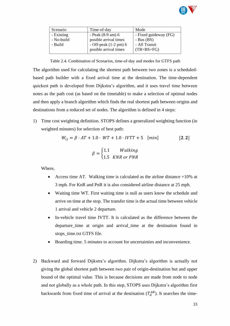
Figure 2.5. Step 2 of schedule-based path algorithm

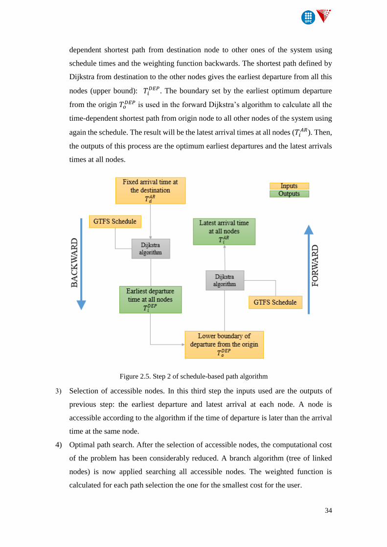
3) Selection of accessible nodes. In this third step the inputs used are the outputs of

previous step: the earliest departure and latest arrival at each node. A node is

accessible according to the algorithm if the time of departure is later than the arrival

time at the same node.

4) Optimal path search. After the selection of accessible nodes, the computational cost

of the problem has been considerably reduced. A branch algorithm (tree of linked

nodes) is now applied searching all accessible nodes. The weighted function is

calculated for each path selection the one for the smallest cost for the user.

35

Table 2.6. Step 3 and 4 of schedule-based path algorithm

The shortest path for all scenarios are skimmed into matrixes that will be the inputs for

mode choice selection and STOPS adaptations.

Travel demand.

In STOPS, there is a specific model developed to obtain person trip tables (results of steps

1 and 2 of traditional four-step models), factoring Year 2000 Census Transportation

Planning products (CTPP) Journey-to-Work (JTW) flows and updating the trips to

account for current and future year demographic growth. This corresponds to the

adaptation process referred in figure 2.7. Results give travel flows for current and future

years classified by purpose and are further split into modes by a nested logit model.

In this part of STOPS models is where parameters adjusted from National calibration are

applied to proceed with the calculations and also, local calibration is applied along

adaptations and mode choice to better fit the forecast trips with actual ridership

experience.

36

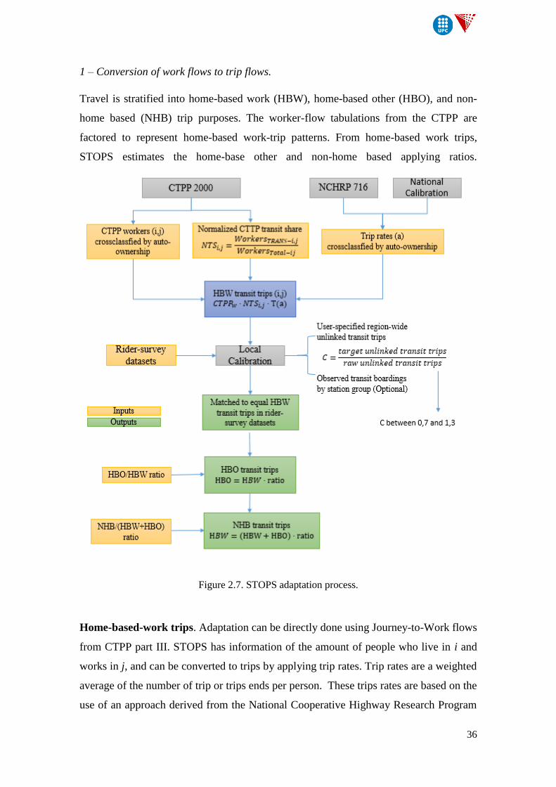
1 – Conversion of work flows to trip flows.

Travel is stratified into home-based work (HBW), home-based other (HBO), and non-

home based (NHB) trip purposes. The worker-flow tabulations from the CTPP are

factored to represent home-based work-trip patterns. From home-based work trips,

STOPS estimates the home-base other and non-home based applying ratios.

Figure 2.7. STOPS adaptation process.

Home-based-work trips. Adaptation can be directly done using Journey-to-Work flows

from CTPP part III. STOPS has information of the amount of people who live in i and

works in j, and can be converted to trips by applying trip rates. Trip rates are a weighted

average of the number of trip or trips ends per person. These trips rates are based on the

use of an approach derived from the National Cooperative Highway Research Program

37

Report 716 (Travel Demand Forecasting: Parameters and Techniques). The HBW trip

rates are cross-classified by auto ownership in the household: 0, 1 and 2 or more per

household.

0 car 1 car 2+ cars

HBW 1.32 1.44 1.56

Table 2.5. Cross-classified trip rates by auto ownership

The total linked trips from i to j are scaled with the normalized CTPP transit shares that

accounts for the people who are using transit. This share is calculated district to district

from CTPP part III where information of the mode of transportation to work is provided

by categories. The concept of linked trips applies for trips from origin to final destination

without accounting for intermediate interchanges or transfers.

The results of total linked transit trips are adjusted then to match transit survey provided

by Transit Agencies. This can be done by correction coefficients to the forecast trips

relating the estimated trips with the actual trips in a region-wide or by station groups. The

coefficient should be in all cases between 0,7 and 1,3. Otherwise it is considered that the

model is not representing well the scenario and further research has to be done.

𝐻𝐵𝑊 𝑡𝑟𝑎𝑛𝑠𝑖𝑡 𝑡𝑟𝑖𝑝𝑠 (𝑖, 𝑗) = 𝐶 · 𝐶𝑇𝑃𝑃𝑤(𝑎) · 𝑁𝑜𝑟𝑚𝑎𝑙𝑖𝑧𝑒𝑑 𝑇𝑆𝑖,𝑗 · 𝑇(𝑎) [𝟐. 𝟑]

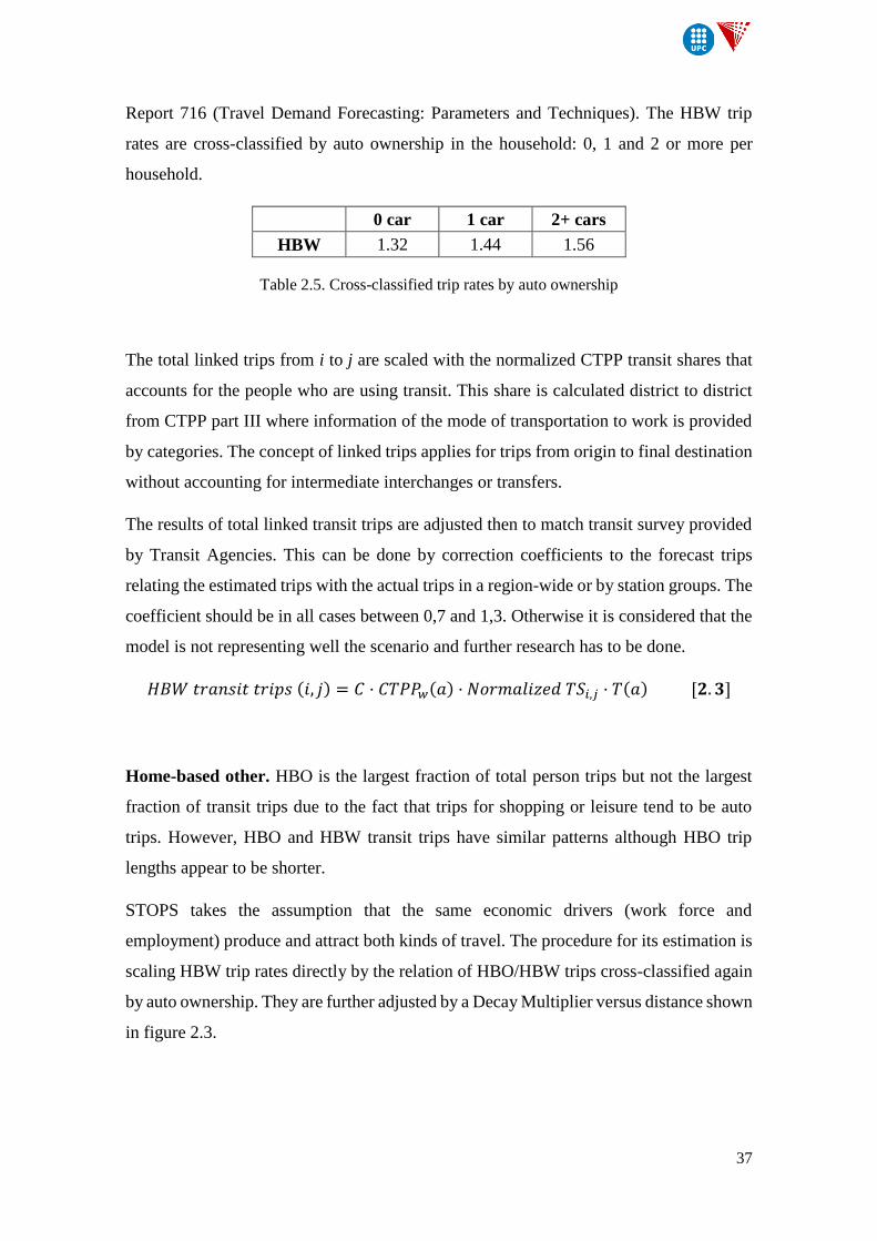
Home-based other. HBO is the largest fraction of total person trips but not the largest

fraction of transit trips due to the fact that trips for shopping or leisure tend to be auto

trips. However, HBO and HBW transit trips have similar patterns although HBO trip

lengths appear to be shorter.

STOPS takes the assumption that the same economic drivers (work force and

employment) produce and attract both kinds of travel. The procedure for its estimation is

scaling HBW trip rates directly by the relation of HBO/HBW trips cross-classified again

by auto ownership. They are further adjusted by a Decay Multiplier versus distance shown

in figure 2.3.

38

Figure 2.8. Model decay factor for HBO trips.

Non-home based. Workers holding jobs in a neighborhood are attracted to economic

activities located in places similar to the residents living in that neighborhood. Non-home

based also appear to have shortest length compared to HBW. The implementation within

STOPS is based on the ratio NHB/(HBW+HBO).

0 car 1 car 2+ cars

HBO 1.78 5.20 5.60

NHB 0.54 2.79 3.00

Table 2.6. Cross-classified trip rates by auto ownership for HBO and NHB.

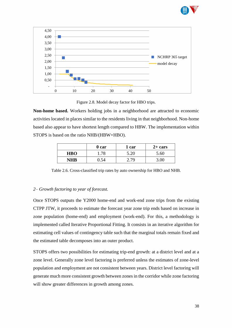
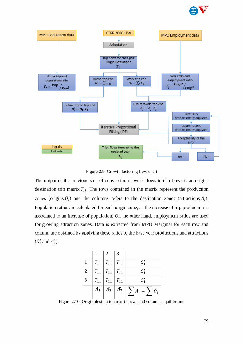
2– Growth factoring to year of forecast.

Once STOPS outputs the Y2000 home-end and work-end zone trips from the existing

CTPP JTW, it proceeds to estimate the forecast year zone trip ends based on increase in

zone population (home-end) and employment (work-end). For this, a methodology is

implemented called Iterative Proportional Fitting. It consists in an iterative algorithm for

estimating cell values of contingency table such that the marginal totals remain fixed and

the estimated table decomposes into an outer product.

STOPS offers two possibilities for estimating trip-end growth: at a district level and at a

zone level. Generally zone level factoring is preferred unless the estimates of zone-level

population and employment are not consistent between years. District level factoring will

generate much more consistent growth between zones in the corridor while zone factoring

will show greater differences in growth among zones.

-

0,50

1,00

1,50

2,00

2,50

3,00

3,50

4,00

4,50

0 10 20 30 40 50

NCHRP 365 target

model decay

39

Figure 2.9. Growth factoring flow chart

The output of the previous step of conversion of work flows to trip flows is an origin-

destination trip matrix 𝑇𝑖𝑗. The rows contained in the matrix represent the production

zones (origins 𝑂𝑖) and the columns refers to the destination zones (attractions 𝐴𝑗).

Population ratios are calculated for each origin zone, as the increase of trip production is

associated to an increase of population. On the other hand, employment ratios are used

for growing attraction zones. Data is extracted from MPO Marginal for each row and

column are obtained by applying these ratios to the base year productions and attractions

(𝑂𝑖′ and 𝐴2

′ ).

1 2 3

1 𝑇11 𝑇11 𝑇11 𝑂1′

2 𝑇11 𝑇11 𝑇11 𝑂1′

3 𝑇11 𝑇11 𝑇11 𝑂1′

𝐴1′ 𝐴2

′ 𝐴3′ ∑ 𝐴𝑗 = ∑ 𝑂𝑖

Figure 2.10. Origin-destination matrix rows and columns equilibrium.

40

The Iterative Proportional Fitting first proceed with row cells matching the sum of row

components with the marginal (future home-trip end 𝑂1′ ) multiplying by a proportional

factor. The same is done for columns (future work-trip end 𝐴1′ ). After several iterations,

if rows and columns give an acceptable error, the final origin-destination matrix is

obtained for the year of interest.

In both base year and future forecast year, the sum of trips productions and trip

productions (sum of row marginal and column marginal) must be equal as it expresses

the equilibrium of the system.

3 – Mode choice

The final goal of travel demand modeling is to assign demand to different transportation

services provided in the area according to the decisions made by the users on the

alternatives. In other words, decisions are based on discrete choices, which means that

each individual has to choose from a set of alternatives which are the modes of

transportation.

Mode choice is based on the principle of utility maximization. This theory stands for the

decision of a specific choice according to a utility expression for each alternative. This

utility expression can be translated as the composed value of the alternative for the user

depending on a series of variables and parameters associated to them. In STOPS the utility

expression is a linear combination of these variables and is deterministic. The highest

utility among all modes, will be the final choice of the user.

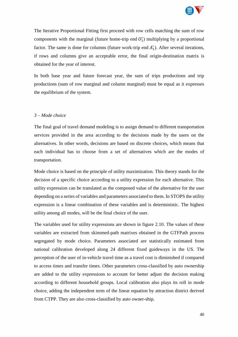
The variables used for utility expressions are shown in figure 2.10. The values of these

variables are extracted from skimmed-path matrixes obtained in the GTFPath process

segregated by mode choice. Parameters associated are statistically estimated from

national calibration developed along 24 different fixed guideways in the US. The

perception of the user of in-vehicle travel time as a travel cost is diminished if compared

to access times and transfer times. Other parameters cross-classified by auto ownership

are added to the utility expressions to account for better adjust the decision making

according to different household groups. Local calibration also plays its roll in mode

choice, adding the independent term of the linear equation by attraction district derived

from CTPP. They are also cross-classified by auto owner-ship.

41

Figure 2.11. Mode choice model for STOPS.

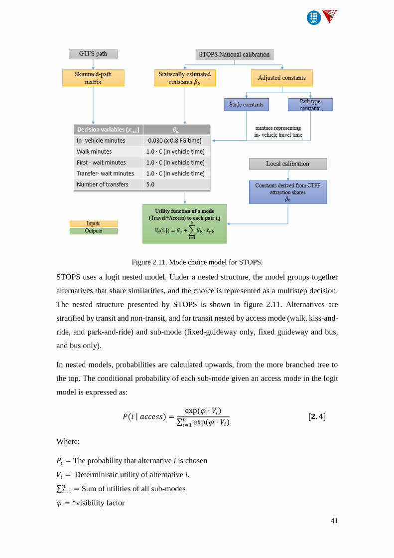
STOPS uses a logit nested model. Under a nested structure, the model groups together

alternatives that share similarities, and the choice is represented as a multistep decision.

The nested structure presented by STOPS is shown in figure 2.11. Alternatives are

stratified by transit and non-transit, and for transit nested by access mode (walk, kiss-and-

ride, and park-and-ride) and sub-mode (fixed-guideway only, fixed guideway and bus,

and bus only).

In nested models, probabilities are calculated upwards, from the more branched tree to

the top. The conditional probability of each sub-mode given an access mode in the logit

model is expressed as:

𝑃(𝑖 | 𝑎𝑐𝑐𝑒𝑠𝑠) =exp (𝜑 · 𝑉𝑖)

∑ exp (𝜑 · 𝑉𝑖)𝑛𝑖=1

[𝟐. 𝟒]

Where:

𝑃𝑖 = The probability that alternative i is chosen

𝑉𝑖 = Deterministic utility of alternative i.

∑ =𝑛𝑖=1 Sum of utilities of all sub-modes

𝜑 = *visibility factor

42

Figure 2.12. STOPS nested structure of alternatives.

The utility of an alternative in an upper level is a function of the utilities of its sub-

alternatives. The utility for a nest includes a variable that represents the expected

maximum utility of all of the alternatives that compose the nest. The variable is known

as the logsum. For the particular tree in STOPS, for transit branch we have that the utility

for different access types is:

𝐼𝑎𝑐𝑐𝑒𝑠𝑠 =1

𝜑· ln (∑ 𝑒𝑥𝑝 (𝜑 · 𝑉𝑖

𝑖

) [𝟐. 𝟓]

With this new variable, STOPS is able to calculate the probability of a specific access

type (KnR, PnR or Walk) given that people are using transit.

𝑃(𝐴𝑐𝑐𝑒𝑠𝑠 | 𝑇𝑟𝑎𝑛𝑠𝑖𝑡) =exp(𝜑 · 𝐼𝑎𝑐𝑐𝑒𝑠𝑠,𝑖)

∑ exp (𝜑 · 𝐼𝑎𝑐𝑐𝑒𝑠𝑠) [𝟐. 𝟔]

Again going up one level, to calculate the probability of people using transit it is used the

same expressions as before. For the non-transit branch the procedure is the same. Finally

it can be obtained the following:

𝐼𝑡𝑟𝑎𝑛𝑠𝑖𝑡 =1

𝜑· ln (∑ exp (𝜑 · 𝐼𝑎𝑐𝑐𝑒𝑠𝑠

𝑖

)) [𝟐. 𝟕]

𝑃(𝑡𝑟𝑎𝑛𝑠𝑖𝑡) =exp(𝜑 · 𝐼𝑇𝑅)

exp(𝜑 · 𝐼𝑇𝑅) + exp(𝜑 · 𝐼𝑁𝑜𝑛𝑇𝑅) [𝟐. 𝟖]

43

From previous expression, transit share for each district can be calculated and adjusted to

match CTPP provided information on modes of transportation. It consists in an iterative

procedure where the parameters to be adjusted are the independent terms of the utility

expression so that they end up reproducing current conditions for the base year.

The outputs of the previous global procedure are a series of tabulations origin to

destination that contain the percentage of shares for each mode classified by auto

ownership. These tables will be the main input for the fourth and last step of the travel

demand model: trip assignment.

2.3.4 Outputs

The last step of the four-step travel demand model corresponds to the trip assignment

both for transit and highway. After mode choice, demand is split into different alternatives

and these demands along the system are loaded into the transit supply. Information about

transit loading is shown as total ridership along a line for peak and off-peak hour and also

station by station loading. About highway assignment the output is the variable Person-

mile Highway Travel and it is not actually a flow of people in a specific link but a usage

of highway supply as a total from zone to zone. For both types of loads, the assignments

are done for current scenario, mainly for calibration aspects, and for future scenarios

which are of the interest of the forecast.

STOPS provides a collection of 1021 tables as an output of the calculation process that

provides information about the parameters and inputs used for the model development

and the results of transit assignment and highway volumes. Main data is collected and

tables help support the story of the project are:

District population and employment for current and future condition based on

MPO data

District-to-district person travel patterns. This output is available for each

scenario, trip purpose, auto ownership level for all modes of transportation.

Transit trip patterns. Available for each scenario, trip purpose, auto ownership

level, access mode, path type. These are referred to linked trips.

44

Transit volumes. The demand in these tables is not distributed from zone-to-zone

but for specific transit lines and stations:

- Station-station unlinked trips available for each scenario, trip purpose,

auto ownership level, access mode, path type.

- Route level ridership

Change in auto mode PMT. Person-miles Highway Travel is estimated for both

current and future conditions and the increment between both is calculated to

account for the impact of the implement transit project in the auto usage.

2.4 Comparison between software and the 4 UTPP

As it has been explain along this chapter, STOPS is a software that is used for project-

evaluation measures such as mobility, estimating trips on project and, indirectly,

environmental impact with the change in auto vehicle-miles traveled. STOPS provides a

simplified method for travel demand forecasting that reduces the considerably the effort

of transit planners with a comfortable level of accuracy of the results.

STOPS was released with two main objectives:

1) To be a first approach to a transit project evaluation as a feasibility study,

understanding better the contributions to mobility and identifying potential

uncertainties and their sources.

2) To be used as a comparison of other forecasts to have a further insight in the

reliability of the results.

In table 2.7. are collected the main differences between the general approach of four-step

travel demand model and STOPS model at each step according to its objectives.

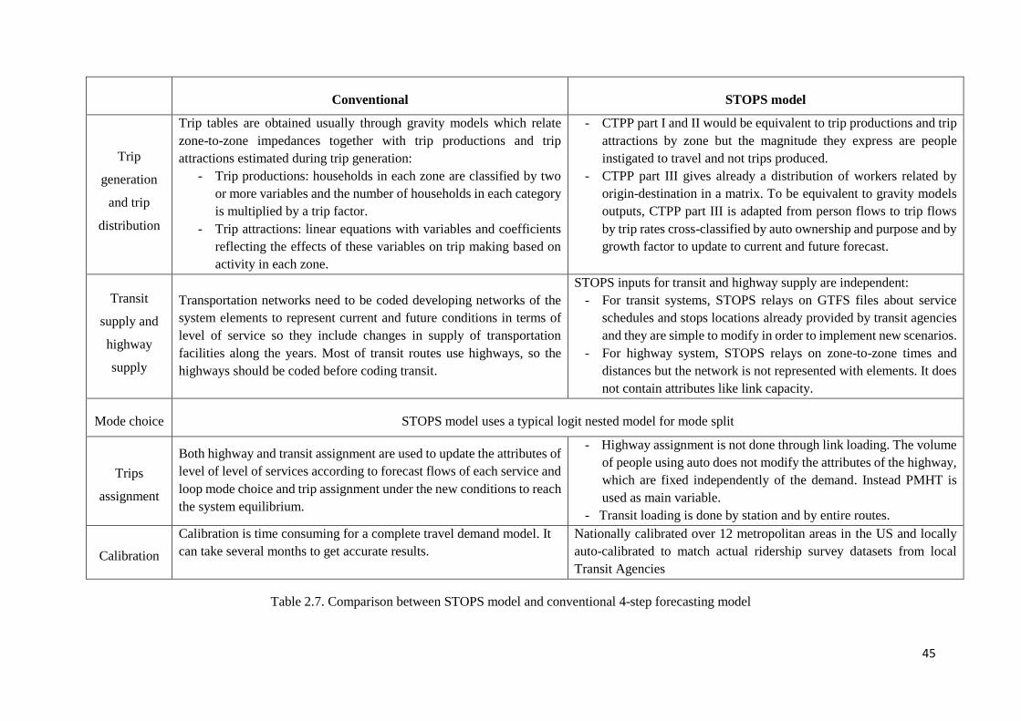
45

Conventional STOPS model

Trip

generation

and trip

distribution

Trip tables are obtained usually through gravity models which relate

zone-to-zone impedances together with trip productions and trip

attractions estimated during trip generation:

- Trip productions: households in each zone are classified by two

or more variables and the number of households in each category

is multiplied by a trip factor.

- Trip attractions: linear equations with variables and coefficients

reflecting the effects of these variables on trip making based on

activity in each zone.

- CTPP part I and II would be equivalent to trip productions and trip

attractions by zone but the magnitude they express are people

instigated to travel and not trips produced.

- CTPP part III gives already a distribution of workers related by

origin-destination in a matrix. To be equivalent to gravity models

outputs, CTPP part III is adapted from person flows to trip flows

by trip rates cross-classified by auto ownership and purpose and by

growth factor to update to current and future forecast.

Transit

supply and

highway

supply

Transportation networks need to be coded developing networks of the

system elements to represent current and future conditions in terms of

level of service so they include changes in supply of transportation

facilities along the years. Most of transit routes use highways, so the

highways should be coded before coding transit.

STOPS inputs for transit and highway supply are independent:

- For transit systems, STOPS relays on GTFS files about service

schedules and stops locations already provided by transit agencies

and they are simple to modify in order to implement new scenarios.

- For highway system, STOPS relays on zone-to-zone times and

distances but the network is not represented with elements. It does

not contain attributes like link capacity.

Mode choice STOPS model uses a typical logit nested model for mode split

Trips

assignment

Both highway and transit assignment are used to update the attributes of

level of level of services according to forecast flows of each service and

loop mode choice and trip assignment under the new conditions to reach

the system equilibrium.

- Highway assignment is not done through link loading. The volume

of people using auto does not modify the attributes of the highway,

which are fixed independently of the demand. Instead PMHT is

used as main variable.

- Transit loading is done by station and by entire routes.

Calibration

Calibration is time consuming for a complete travel demand model. It

can take several months to get accurate results.

Nationally calibrated over 12 metropolitan areas in the US and locally

auto-calibrated to match actual ridership survey datasets from local

Transit Agencies

Table 2.7. Comparison between STOPS model and conventional 4-step forecasting model

46

CH

AP

TER

3

DETERMINATION OF CTA PARK-AND-RIDE

PRICE ELASTICITIES

47

3. DETERMINATION OF CTA PARK-AND-RIDE

PRICE ELASTICTIES

3.1 Introduction

Park-and-ride facilities are important components of major urban systems across North

America and around the world. They act as a key bridge between road networks and

transit systems as well as playing a core role in facilitating cross-modal integration and

in providing access to transit for users who may not otherwise consider transit as a travel

alternative. Modal integration to facilitate multiple options for travel is often desirable

objective in urban transportation planning. This is the reason why Park-and-ride facilities

are considered as key transit-oriented facilities although an abuse in density throughout

the territory may cause negative effect, promoting private transportation as a mode of

access to transit trip or services around like churches, dining venues or other evening

entertainment.

The main reason of existence of these facilities is related to the high costs of parking at

user destinations, such as downtown. The decision of using a park-and-ride is more cost-

effective for most of the users who have a long commute and work in the city center. A

part from the economic cost for the user, park-and-ride have a real effect on highway

congestion, reducing traffic in main roads connecting to downtown at peak-commute.

Well-designed park-and-ride facilities can efficiently increase the capacity of the whole

urban transportation system and optimally utilize transit facilities (Garcia and Marín

2002). All these advantages make Park-and-Ride a high-potential facility that is becoming

more popular at the time of facing sustainable issues in big cities.

However, due to its increased popularity since its implementation, park-and-ride

management has been necessary to control its operation through strategies and charging

policies. Parking charges at park-and-ride lots are meant to cover some of the cost of

maintenance and operations and in a secondary stage, are set to manage the supply at

these facilities. Therefore, introducing parking charges has been a common practice for

many transit agencies However, the basic principle of park-and-ride for a correct

functionality, is that cost to park and take transit must be less than the cost to drive and

park downtown, and this has to be reflected in parking rates.

48

The objective of this case study is to investigate the effect of increasing parking charges

at park-and-ride stations on mode choice for current park-and-ride users and the impact

in the whole transit system in the city of Chicago. The case study is focused on 17 park-

and-ride associated to the Chicago Transit Authority (CTA) “L” Rail Lines that are spread

along the metropolitan area. The Metropolitan Area of Chicago has 9,4 millions of

inhabitants in a surface of 10.856 square miles and is one of the metropolitan areas in the

US with greater socioeconomic contrast from zone to zone. The goal of the research is

determining the direct and cross elasticity as a main index to reflect the effect of

increasing parking charges and discuss the results according to land use and

socioeconomic factors across the territory.

To address this objective, STOPS software will be used as a tool for transportation

demand forecasting in urban systems with a relatively simple and straightforward

implementation, introduced in Chapter 2. The collection of the inputs for the city of

Chicago and the implementation of a model for introducing CTA parking costs in the

simulation, will lead to determine the demand at each park-and-ride and at other

complementary modes, for different parking pricing scenarios. STOPS outputs will allow

to calculate the price elasticity after a sensitivity analysis.

This chapter is organized as follows: in the first part it is introduced the theory of price

elasticity and how it applies to transportation systems and the way they are calculated.

This is followed by a section which describes in detail the inputs needed for STOPS

simulation: in particular for the Chicago Metropolitan Area (socioeconomics, population,

employment, transit systems,..) extracted from the Regional Transit Authority (RTA) and

the inputs regarding parking charges according to a pricing model calibrated and validated

through real CTA data. The later sections present the results obtained for each of the 17

park-and-ride stations and districts, and they are compared with other two studies

published regarding the park-and-ride elasticity estimation. The first of them is a study

carried out in the Greater Vancouver Region, which determined the probability density

function of the elasticities obtained for the 14 park-and-ride associated to the main rail

network. The second is a reference paper in transportation system elasticity’s which

provides reference values of cross-elasticity’s for increasing parking charges regarding to

other modes of transportation. The chapter concludes with a spatial analysis based on

land use and socioeconomic parameters in order to find a relationship between these

variables and the results.

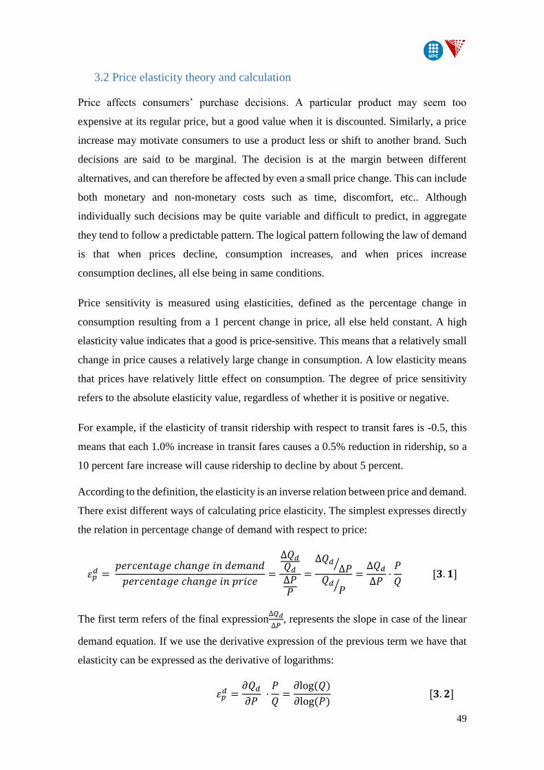
49

3.2 Price elasticity theory and calculation

Price affects consumers’ purchase decisions. A particular product may seem too

expensive at its regular price, but a good value when it is discounted. Similarly, a price

increase may motivate consumers to use a product less or shift to another brand. Such

decisions are said to be marginal. The decision is at the margin between different

alternatives, and can therefore be affected by even a small price change. This can include

both monetary and non-monetary costs such as time, discomfort, etc.. Although

individually such decisions may be quite variable and difficult to predict, in aggregate

they tend to follow a predictable pattern. The logical pattern following the law of demand

is that when prices decline, consumption increases, and when prices increase

consumption declines, all else being in same conditions.

Price sensitivity is measured using elasticities, defined as the percentage change in

consumption resulting from a 1 percent change in price, all else held constant. A high

elasticity value indicates that a good is price-sensitive. This means that a relatively small

change in price causes a relatively large change in consumption. A low elasticity means

that prices have relatively little effect on consumption. The degree of price sensitivity

refers to the absolute elasticity value, regardless of whether it is positive or negative.

For example, if the elasticity of transit ridership with respect to transit fares is -0.5, this

means that each 1.0% increase in transit fares causes a 0.5% reduction in ridership, so a

10 percent fare increase will cause ridership to decline by about 5 percent.

According to the definition, the elasticity is an inverse relation between price and demand.

There exist different ways of calculating price elasticity. The simplest expresses directly

the relation in percentage change of demand with respect to price:

𝜀𝑝𝑑 =

𝑝𝑒𝑟𝑐𝑒𝑛𝑡𝑎𝑔𝑒 𝑐ℎ𝑎𝑛𝑔𝑒 𝑖𝑛 𝑑𝑒𝑚𝑎𝑛𝑑

𝑝𝑒𝑟𝑐𝑒𝑛𝑡𝑎𝑔𝑒 𝑐ℎ𝑎𝑛𝑔𝑒 𝑖𝑛 𝑝𝑟𝑖𝑐𝑒=

∆𝑄𝑑

𝑄𝑑

∆𝑃𝑃

=

∆𝑄𝑑∆𝑃⁄

𝑄𝑑𝑃⁄

=∆𝑄𝑑

∆𝑃·

𝑃

𝑄 [𝟑. 𝟏]

The first term refers of the final expression∆𝑄𝑑

∆𝑃, represents the slope in case of the linear

demand equation. If we use the derivative expression of the previous term we have that

elasticity can be expressed as the derivative of logarithms:

𝜀𝑝𝑑 =

𝜕𝑄𝑑

𝜕𝑃 ·

𝑃

𝑄=

𝜕log (𝑄)

𝜕log (𝑃) [𝟑. 𝟐]

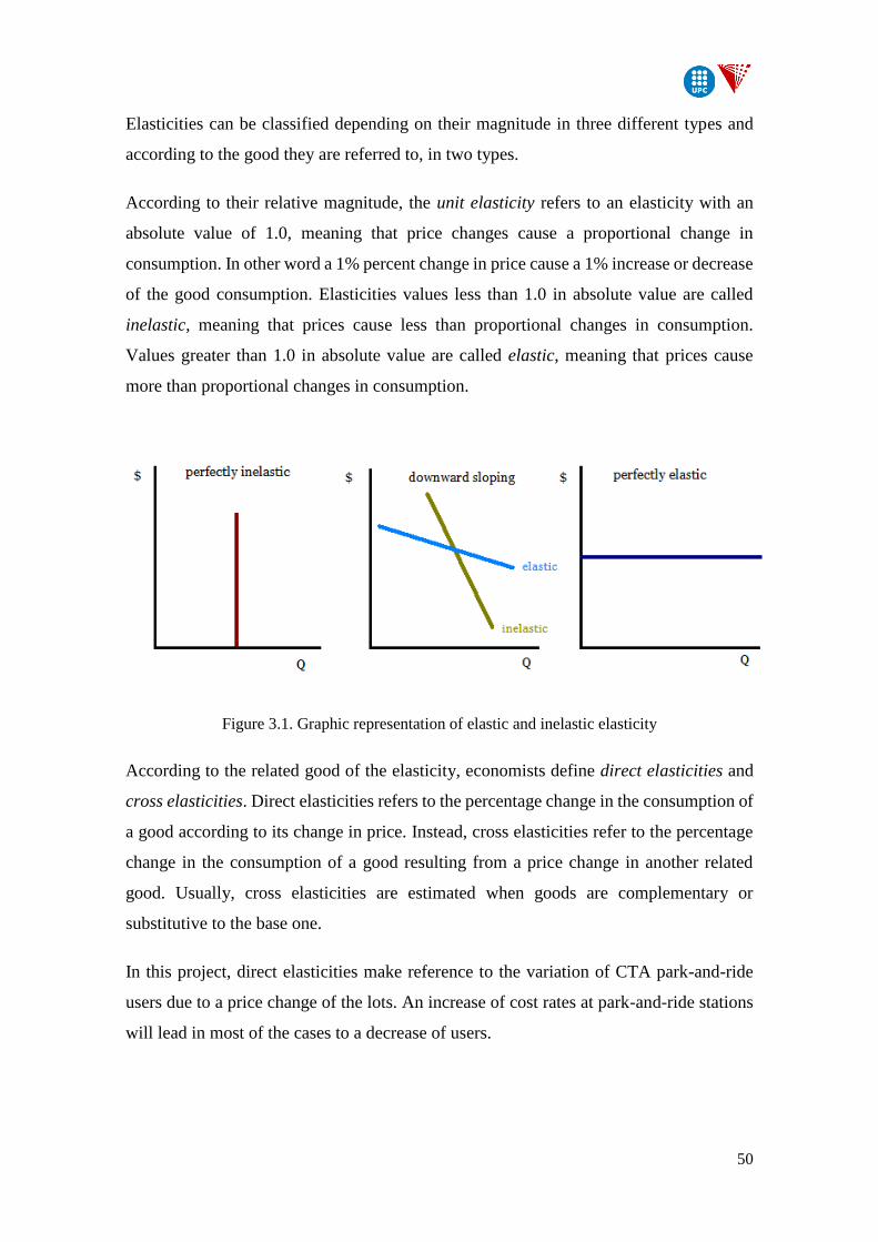
50

Elasticities can be classified depending on their magnitude in three different types and

according to the good they are referred to, in two types.

According to their relative magnitude, the unit elasticity refers to an elasticity with an

absolute value of 1.0, meaning that price changes cause a proportional change in

consumption. In other word a 1% percent change in price cause a 1% increase or decrease

of the good consumption. Elasticities values less than 1.0 in absolute value are called

inelastic, meaning that prices cause less than proportional changes in consumption.

Values greater than 1.0 in absolute value are called elastic, meaning that prices cause

more than proportional changes in consumption.

Figure 3.1. Graphic representation of elastic and inelastic elasticity

According to the related good of the elasticity, economists define direct elasticities and

cross elasticities. Direct elasticities refers to the percentage change in the consumption of

a good according to its change in price. Instead, cross elasticities refer to the percentage

change in the consumption of a good resulting from a price change in another related

good. Usually, cross elasticities are estimated when goods are complementary or

substitutive to the base one.

In this project, direct elasticities make reference to the variation of CTA park-and-ride

users due to a price change of the lots. An increase of cost rates at park-and-ride stations

will lead in most of the cases to a decrease of users.

51

Cross elasticities for increasing price of park-and-ride may reflect the affection in other

complementary modes to car as an access choice to transit. In fact, those users who shift

to another way of transportation due to the increase of cost have two differentiate options:

a) Change the access mode, to get to the same station (or nearer station) and use rail

as a final mode to get to their destination. This includes, basically, shifting car

mode by walking, ridesharing or bus which has connection with rail, used as an

access mode.

b) Change from mixed-mode trip to single-mode trip. This includes shifting to all

way car or all way transit (only bus or only train).

The most beneficial complementary modes are those related to transit, being both

beneficial as access mode or all way transit, and also walking or cycle modes. On the

other hand, the increase of car trips in the urban system will lead to an increasing

congestion of the network producing negative environmental effects related to emissions.

Price elasticities have many applications in transportation planning. In particular for this

project, the determination of direct elasticities will provide information about the price

sensitivity of each park-and-ride related to CTA rail network and the cross elasticities,

the impact in the transportation systems of Chicago. Results will help to decide how the

different networks performance can be improved by adjusting park-and-ride pricing

according to their response.

Factors affecting price elasticities:

Price elasticities may depend locally on different factors that can affect user decisions.

They can vary depending on how elasticities are defined, type of mode or service affected,

category of customer, quality of alternatives and other market factors. Some of the factors

are described below:

User type: Transit dependent riders are generally less price sensitive than choice

or discretionary riders (who have the option of using automobile for that trip).

Trip type. Non-commute trips tend to be more price sensitive than commute trips.

Elasticities for off-peak transit travel are typically 1.5 to 2 time higher than peak-

period elasticities, because peak-period travel basically consist on home-based

work trips.

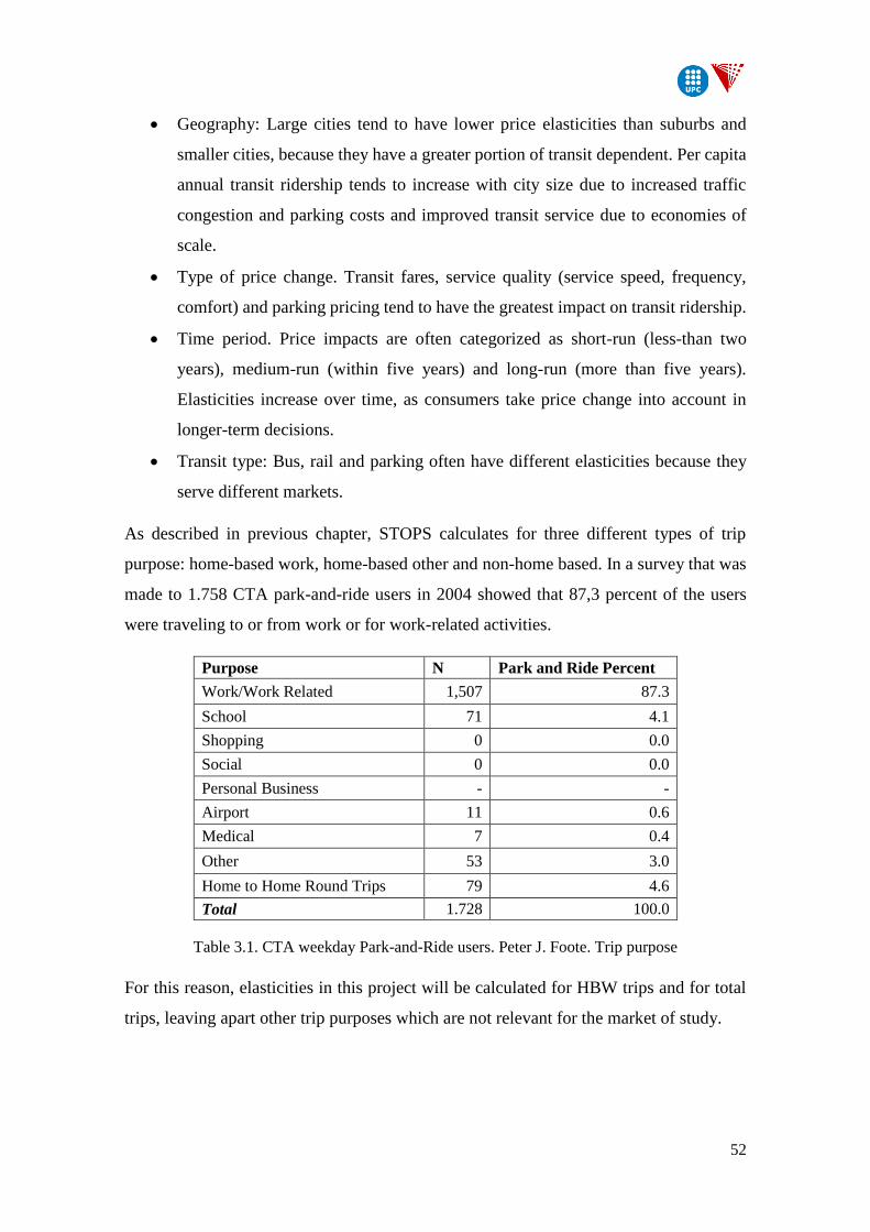
52

Geography: Large cities tend to have lower price elasticities than suburbs and

smaller cities, because they have a greater portion of transit dependent. Per capita

annual transit ridership tends to increase with city size due to increased traffic

congestion and parking costs and improved transit service due to economies of

scale.

Type of price change. Transit fares, service quality (service speed, frequency,

comfort) and parking pricing tend to have the greatest impact on transit ridership.

Time period. Price impacts are often categorized as short-run (less-than two

years), medium-run (within five years) and long-run (more than five years).

Elasticities increase over time, as consumers take price change into account in

longer-term decisions.

Transit type: Bus, rail and parking often have different elasticities because they

serve different markets.

As described in previous chapter, STOPS calculates for three different types of trip

purpose: home-based work, home-based other and non-home based. In a survey that was

made to 1.758 CTA park-and-ride users in 2004 showed that 87,3 percent of the users

were traveling to or from work or for work-related activities.

Purpose N Park and Ride Percent

Work/Work Related 1,507 87.3

School 71 4.1

Shopping 0 0.0

Social 0 0.0

Personal Business - -

Airport 11 0.6

Medical 7 0.4

Other 53 3.0

Home to Home Round Trips 79 4.6

Total 1.728 100.0

Table 3.1. CTA weekday Park-and-Ride users. Peter J. Foote. Trip purpose

For this reason, elasticities in this project will be calculated for HBW trips and for total

trips, leaving apart other trip purposes which are not relevant for the market of study.

53

3.3 Description of the inputs

This section is organized in two parts.

The first one pretends to describe the inputs needed for running STOPS applying for the

project that is presented for the city of Chicago. They were accurately prepared by the

Regional Transportation Authority (RTA) of Chicago with to objective of facilitating the

work for public and private entities who are willing to use STOPS as a tool to implement

a new project in the city.

The second part focuses in particular on the development and implementation of the

inputs released by RTA to reflect the case study of this project. The main explanation

makes reference to the modification of the GTFS files regarding the information about

the Park-and-Ride associated to the CTA rail lines. To do that, a model to transform

pricing cost to time cost for users, is calibrated and validated to meet actual CTA demand

at park-and-ride during weekdays for 2015.

3.3.1 Regional Transportation Authority’s regionally calibrated STOPS inputs

The RTA is the financial and oversight body for the three principal transit agencies in

northeastern Illinois, serving Cook, DuPage, Kane, Lake, McHenry and Will counties. In

November 2015, they released a package of inputs for STOPS which are downloadable

from their webpage.

These files represent a consistent set of inputs representing a “base case” scenario for the

entire RTA region within the STOPS environment. From this base scenario, transit

modelers are able to code new build and no-build scenarios with significant reduction in

setup and calibration time and obtain reliable estimates of demand in the main transit

systems across the Chicago region.

The set of inputs include socioeconomic and demographic data at different geographic

levels to the choice of the user, and the files regarding the network configuration and

operation of the services provided by the three principal transit agencies in the

Metropolitan Area of Chicago: CTA, Metra and PACE. It also includes a zone-to-zone

impedance matrix for auto travel and a district definition, grouping geographic elements

which have similar transportation patterns.

54

CTPP 2000:

CTPP tables from Part I, Part II and Part III are included in the set of RTA’s inputs. The

extension of these tables does not only cover Illinois area but also includes part of

Wisconsin and Indiana socioeconomic information. The reason for this is that one of the

transit systems covering the Chicago Metropolitan Area which is the Metra rail, grows

from Chicago downtown towards the suburbs, reaching at some branches these two States

along its path. This data coverage is necessary to well represent the context of the system

in terms of ridership.

For this project in particular, although the analysis is only focus on the park-and-ride

associated to the CTA “L” Rail Line, which has less extensions, the representation of the

other transportation systems are needed to obtain accurate and realistic results.

Demographic data:

MPO Population and Employment data for past, current and future years are provided by

the Chicago Metropolitan Area for Planning’s regional model. The file organizes that

Population and Employment Data in shapefile database fields for the following years:

2000 (used to relate to 2000 CTPP data), 2010, 2015, 2025, 2030, 2040.

The geographic level of these data can be found for Transport Analysis Zones (TAZ) and

TRACTS defined for the Chicago Area by CMAP.

For this project where the objective is to determine the park-and-ride price elasticities,

the year of reference to calculate them is 2015. This is the latest year with real information

regarding population and employment and a year from which socioeconomic data exists

and can be extracted with the purpose of analysis. Then, from RTA inputs, it will only be

needed data regarding 2000 and 2015 to update CTPP 2000 tables to that year.

Regarding the geographic level of the data, it has been decided to work at the TRACT

level, as the project that it is implemented in STOPS is at a metropolitan area level, which

means that the detail of a specific zone of the city is not needed because the area of the

influence of the project is much wider. It is also important to highlight that the

computational cost for STOPS using a geographic grid such TAZ’s is much higher, which

is not of our interest, taking into account the purpose of this project of doing a sensibility

analysis. This geographical level is defined in both demographic and CTPP data.

55

GTFS files:

The three transit agencies that operate in the Chicago Area are the Chicago Transit

Authority (CTA), Metra and PACE, and all three are represented in the GTFS format to

be used as an input for STOPS. GTFS files include transportation schedules and the

spatial information associated for all of the services offered by the agencies.

1. Chicago Transit Authority:

CTA operates the nation’s second largest public transportation system. It covers the City

of Chicago and 40 neighboring communities. CTA provides 1.64 million rides on an

average weekday, accounting for over 80% of all transit trips taken in the six-county

Chicago metropolitan region. In the present, CTA is providing services by two modes:

bus and rail.

Chicago Transit Authority represents the main bus operator, providing service with 140

routes. Buses make over 25.000 trips daily, and serve nearly 12.000 bus stops throughout

the region. CTA bus routes serve communities locally, move people across town, and a

number of express services are provided. Several routes also provide 24-hour service.

The rail service offered by CTA consists of train lines spanning the city and neighboring

communities and is known as “The ‘L’”. It has a radial coverture over the territory,

growing from the city center of Chicago (The Loop) and being extended up to 15 miles

from there. The service provided is described as “heavy rail rapid transit”, also referred

to as “subway” or “metro” in many parts of the world. The system has today eight rapid

transit routes identified with colors and consists of 145 stations over approximately 241.1

miles track. Part of the lines run above ground, in subway tunnels and tubes, as well as at

grade or in expressway medians.

GTFS inputs for CTA include all required text files described in chapter 3: agency.txt,

stops.txt, routes.txt, trips.txt, stops_times.txt, calendar.txt. A part from those, it is also

included the optional files about transfer and shapes and park-and-ride stations. All of

them are presented in three different folders representing the three different scenarios:

Existing, No-Build and Build scenarios, which in case of the base scenario provided by

RTA, the three of them are the same as any project is still implemented.

56

The last of the text files listed above is of special interest for this project. RTA include a

GTFS file describing some of the Park-and-Ride associated to the network: in total just 7

out of the 17 existing. In the second part of this section it will be described the existing

park-and-ride, which of them are implemented and what is the procedure followed to

implement the others not yet programmed.

The CTA network is shown in figure 3.2, with all the rail lines and bus stops across the

City of Chicago. It is also shown the location of the 17 park-and-ride locations.

2. Metra:

Metra is a commuter railroad in the Chicago metropolitan area which operates over 241

stations on 11 different rail lines. It is the fourth busiest commuter rail system in the

United States by ridership and the largest rail system outside the New York City

metropolitan area. There were 83.4 million passenger rides in 2014.

The structure of this network is very similar to the CTA “L” rail with a radial shape, but

a bigger scale, connection with many municipalities from 6 different counties. Metra has

also park-and-ride facilities along its stations. Most of the municipalities have one.

However, there’s no interception between park-and-ride facilities from Metra and those

of CTA.

The extension of the network is shown in figure 3.3, where it can be observed that the

average coverage radius from the Chicago Loop is approximately three times the

coverage of CTA rail. They type of users attracted by each operator are significantly

different.

3. PACE.

PACE is the suburban bus division of the Regional Transportation Authority in the

Chicago metropolitan area. It was created in 1983 and nowadays is safely and efficiently

moving people to work, school and other regional destinations, covering 284

municipalities in Cook, Will, Du Page, Kane, Lake and McHenry counties, approximately

3.446 square miles. Pace serves tens of thousands of daily riders.

This operator is the backbone of Chicago’s suburbs. Although PACE has a coverage also

in the Cook County where it coexists with CTA buses, these last ones are predominant

and attract the major ridership in the city of Chicago.

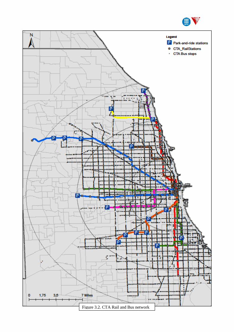
57

Figure 3.2. CTA Rail and Bus network

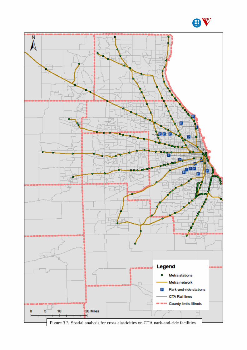
58

Figure 3.3. Spatial analysis for cross elasticities on CTA park-and-ride facilities

59

Zone-to-zone automobile travel times and distances.

The Metropolitan Planning Organization of Chicago, which is CMAP, is the responsible

for regional travel demand forecasts. Together with real data extracted from the road

network they are able to provide information about auto travel impedances from zone to

zone in the metropolitan area. This information is collected in a huge matrix that for the

area of this study is a 1961x1961 (1961 zones) for each of the variables: distance between

zones and speeds for peak and off-peak periods.

The structure of the road network connecting to the center of the city is shown in figure

3.4. Similar to Metra and CTA rail networks, it has a radial shape in the immediate

surroundings of downtown, becoming a grid structure outside the City of Chicago.

District definition:

STOPS allows the user to group geographic units to create districts with two objectives.

The first one is to calibrate regional ridership at this level. The second is to group results

in matrixes district-to-district as outputs of the simulation. RTA, when releasing the

package of inputs, included a district proposal open to be modified according to user

criteria and particularities of the project.

The original district definition for the region was made by a spatial grouping of zones

with similar transportation patterns in order to add consistency in the regional calibration

process. ArcGIS was used as tool to perform the spatial grouping. It consisted in 34 areas

grouped by mode share similarity from the 2000 CTPP

For this particular project, original districts are further broken down by reorganizing and

grouping them with other geographical units to our interest. The objective is to define

districts containing CTA park-and-ride facilities with the following criteria:

- Consecutive facilities belonging to the same rail line, except for the Purple and

Yellow lines that are considered together as a bifurcation of the red line.

- Facilities with similar spatial relations such as distance between them or proximity

to city center.

The result is shown in figure 3.5, where only districts containing park-and-ride facilities

are colored, except for the Loop districts which is in white color to limit the downtown

area. In total there are defined 9 districts containing the 17 parking facilities.

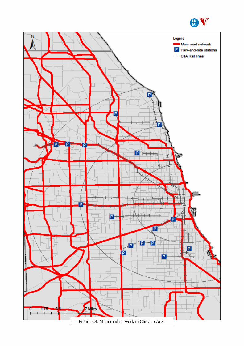
60

Figure 3.4. Main road network in Chicago Area

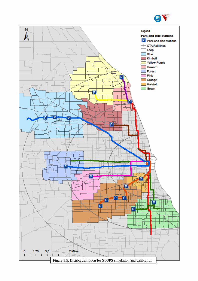
61

Figure 3.5. District definition for STOPS simulation and calibration

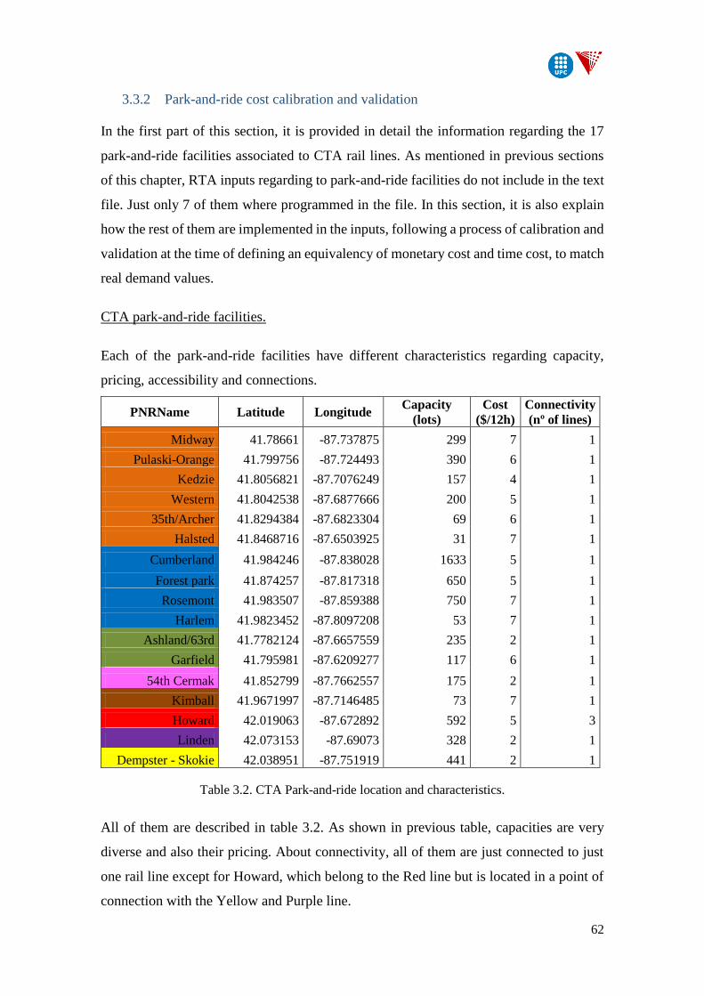
62

3.3.2 Park-and-ride cost calibration and validation

In the first part of this section, it is provided in detail the information regarding the 17

park-and-ride facilities associated to CTA rail lines. As mentioned in previous sections

of this chapter, RTA inputs regarding to park-and-ride facilities do not include in the text

file. Just only 7 of them where programmed in the file. In this section, it is also explain

how the rest of them are implemented in the inputs, following a process of calibration and

validation at the time of defining an equivalency of monetary cost and time cost, to match

real demand values.

CTA park-and-ride facilities.

Each of the park-and-ride facilities have different characteristics regarding capacity,

pricing, accessibility and connections.

PNRName Latitude Longitude Capacity

(lots)

Cost

($/12h)

Connectivity

(nº of lines)

Midway 41.78661 -87.737875 299 7 1

Pulaski-Orange 41.799756 -87.724493 390 6 1

Kedzie 41.8056821 -87.7076249 157 4 1

Western 41.8042538 -87.6877666 200 5 1

35th/Archer 41.8294384 -87.6823304 69 6 1

Halsted 41.8468716 -87.6503925 31 7 1

Cumberland 41.984246 -87.838028 1633 5 1

Forest park 41.874257 -87.817318 650 5 1

Rosemont 41.983507 -87.859388 750 7 1

Harlem 41.9823452 -87.8097208 53 7 1

Ashland/63rd 41.7782124 -87.6657559 235 2 1

Garfield 41.795981 -87.6209277 117 6 1

54th Cermak 41.852799 -87.7662557 175 2 1

Kimball 41.9671997 -87.7146485 73 7 1

Howard 42.019063 -87.672892 592 5 3

Linden 42.073153 -87.69073 328 2 1

Dempster - Skokie 42.038951 -87.751919 441 2 1

Table 3.2. CTA Park-and-ride location and characteristics.

All of them are described in table 3.2. As shown in previous table, capacities are very

diverse and also their pricing. About connectivity, all of them are just connected to just

one rail line except for Howard, which belong to the Red line but is located in a point of

connection with the Yellow and Purple line.

63

Regarding to the cost, CTA offers different type of parking rates depending on the amount

of time of utilization. All of them have pricing rates for 12-hour utilization of the lot. In

addition, some of them have also other type of rates for higher amount of hours (14h, 16h,

18h, 24h) and usually they also offer monthly rates for those who are habitual. Rates also

differ from weekdays and weekends in some cases. For the purpose of this study, it has

been decided to use the 12-hour utilization rate for each of the park-and-rides as it is the

common type of rate among them. All the rates are for 2015, the year of study.

Parking pricing conversion model.

GTFS text file containing park-and-ride network configuration, has a row in its code for

each of the facilities. In each row, separated by comas, are defined the attributes which

describe the park-and-ride inputs. Those are the name of the facility, the latitude and

longitude, the type of park-and-ride and the cost. Only 7 out of a total of 17 are defined

by RTA. These are: Dempster-Skokie, Midway, Pulaski, Howard, Linden,

Cumberland and Forest park.

STOPS defines 4 different types of park-and-ride facilities depending on their radius of

influence. The 7 park-and-ride already coded, were defined as type 4, which makes

references to a radius of influence of 3 miles. RTA limited the area of impact of CTA

park-and-ride to a 3 mile radius because of the context of the rail line, understood as a

relative urban network, attracting users from the surrounding neighborhoods but not

actually people from further suburbs.

The main issue of the implementation is related to the cost that STOPS uses to penalize

the utilization of the lots reflecting the rates of each of them. As it is explained in chapter

2, users decisions are modeled by a logit nested model which is based in an utility function

that accounts cost in time units. To calculate the cost in time units representing the

monetary cost and other variables that affect the decision of the users, it has been used a

model which relays on the time penalty applied to the already implemented facilities and

a relation between these and the main affecting variables has been established through a

multi linear regression model.

The calibration of this model implemented by RTA was based on the variables that

affected the users at the time to decide which of the options is best cost-effective for them.

According to STOPS user guide for Chicago Area, this calibration took into account the

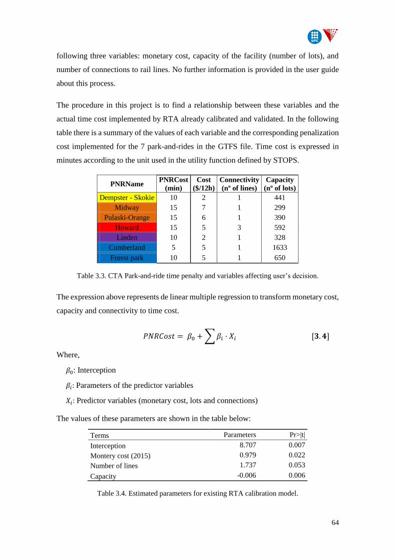
64

following three variables: monetary cost, capacity of the facility (number of lots), and

number of connections to rail lines. No further information is provided in the user guide

about this process.

The procedure in this project is to find a relationship between these variables and the

actual time cost implemented by RTA already calibrated and validated. In the following

table there is a summary of the values of each variable and the corresponding penalization

cost implemented for the 7 park-and-rides in the GTFS file. Time cost is expressed in

minutes according to the unit used in the utility function defined by STOPS.

PNRName PNRCost

(min)

Cost

($/12h)

Connectivity

(nº of lines)

Capacity

(nº of lots)

Dempster - Skokie 10 2 1 441

Midway 15 7 1 299

Pulaski-Orange 15 6 1 390

Howard 15 5 3 592

Linden 10 2 1 328

Cumberland 5 5 1 1633

Forest park 10 5 1 650

Table 3.3. CTA Park-and-ride time penalty and variables affecting user’s decision.

The expression above represents de linear multiple regression to transform monetary cost,

capacity and connectivity to time cost.

𝑃𝑁𝑅𝐶𝑜𝑠𝑡 = 𝛽0 + ∑ 𝛽𝑖 · 𝑋𝑖 [𝟑. 𝟒]

Where,

𝛽0: Interception

𝛽𝑖: Parameters of the predictor variables

𝑋𝑖: Predictor variables (monetary cost, lots and connections)

The values of these parameters are shown in the table below:

Terms Parameters Pr>|t|

Interception 8.707 0.007

Montery cost (2015) 0.979 0.022

Number of lines 1.737 0.053

Capacity -0.006 0.006

Table 3.4. Estimated parameters for existing RTA calibration model.

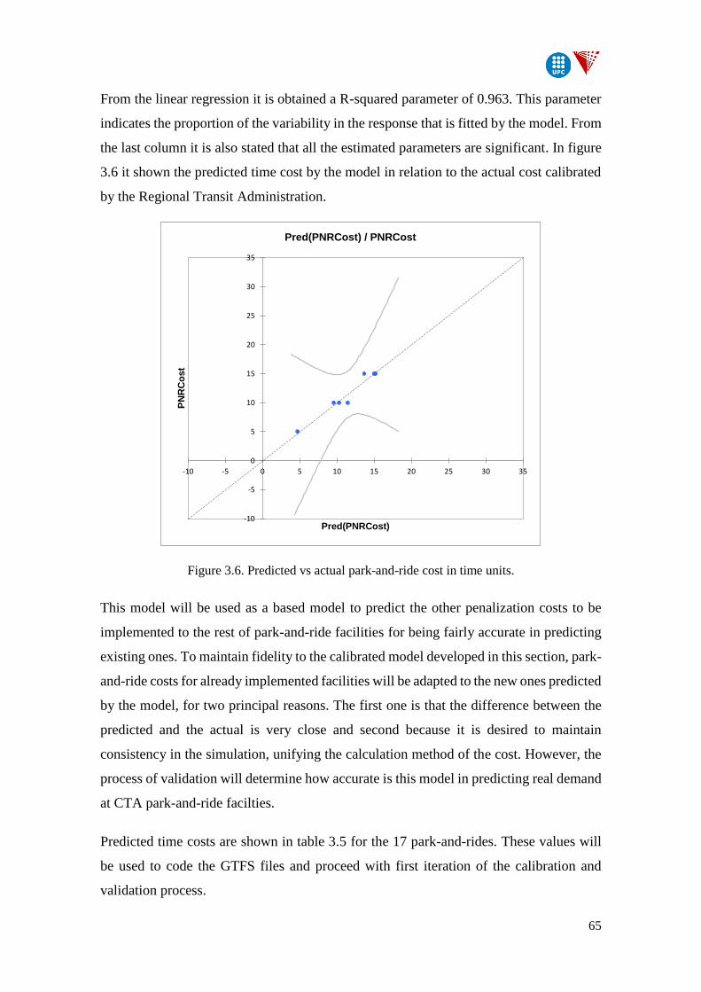
65

From the linear regression it is obtained a R-squared parameter of 0.963. This parameter

indicates the proportion of the variability in the response that is fitted by the model. From

the last column it is also stated that all the estimated parameters are significant. In figure

3.6 it shown the predicted time cost by the model in relation to the actual cost calibrated

by the Regional Transit Administration.

Figure 3.6. Predicted vs actual park-and-ride cost in time units.

This model will be used as a based model to predict the other penalization costs to be

implemented to the rest of park-and-ride facilities for being fairly accurate in predicting

existing ones. To maintain fidelity to the calibrated model developed in this section, park-

and-ride costs for already implemented facilities will be adapted to the new ones predicted

by the model, for two principal reasons. The first one is that the difference between the

predicted and the actual is very close and second because it is desired to maintain

consistency in the simulation, unifying the calculation method of the cost. However, the

process of validation will determine how accurate is this model in predicting real demand

at CTA park-and-ride facilties.

Predicted time costs are shown in table 3.5 for the 17 park-and-rides. These values will

be used to code the GTFS files and proceed with first iteration of the calibration and

validation process.

-10

-5

0

5

10

15

20

25

30

35

-10 -5 0 5 10 15 20 25 30 35

PN

RC

os

t

Pred(PNRCost)

Pred(PNRCost) / PNRCost

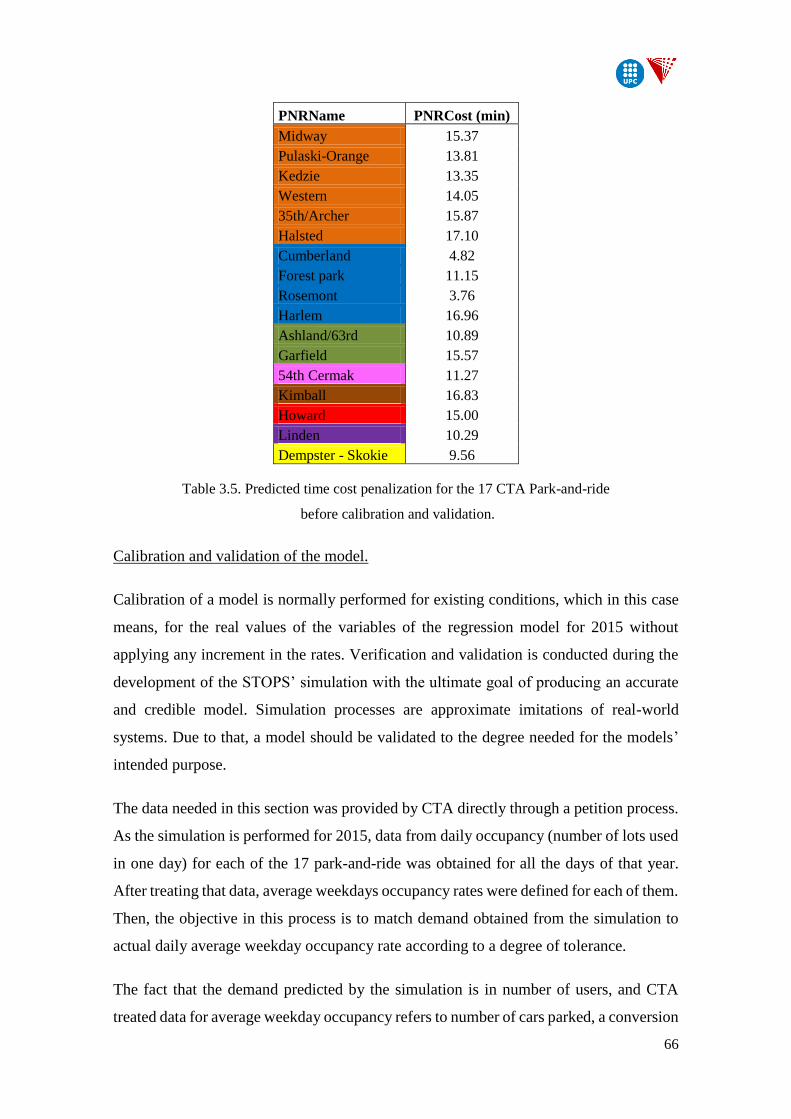
66

PNRName PNRCost (min)

Midway 15.37

Pulaski-Orange 13.81

Kedzie 13.35

Western 14.05

35th/Archer 15.87

Halsted 17.10

Cumberland 4.82

Forest park 11.15

Rosemont 3.76

Harlem 16.96

Ashland/63rd 10.89

Garfield 15.57

54th Cermak 11.27

Kimball 16.83

Howard 15.00

Linden 10.29

Dempster - Skokie 9.56

Table 3.5. Predicted time cost penalization for the 17 CTA Park-and-ride

before calibration and validation.

Calibration and validation of the model.

Calibration of a model is normally performed for existing conditions, which in this case

means, for the real values of the variables of the regression model for 2015 without

applying any increment in the rates. Verification and validation is conducted during the

development of the STOPS’ simulation with the ultimate goal of producing an accurate

and credible model. Simulation processes are approximate imitations of real-world

systems. Due to that, a model should be validated to the degree needed for the models’

intended purpose.

The data needed in this section was provided by CTA directly through a petition process.

As the simulation is performed for 2015, data from daily occupancy (number of lots used

in one day) for each of the 17 park-and-ride was obtained for all the days of that year.

After treating that data, average weekdays occupancy rates were defined for each of them.

Then, the objective in this process is to match demand obtained from the simulation to

actual daily average weekday occupancy rate according to a degree of tolerance.

The fact that the demand predicted by the simulation is in number of users, and CTA

treated data for average weekday occupancy refers to number of cars parked, a conversion

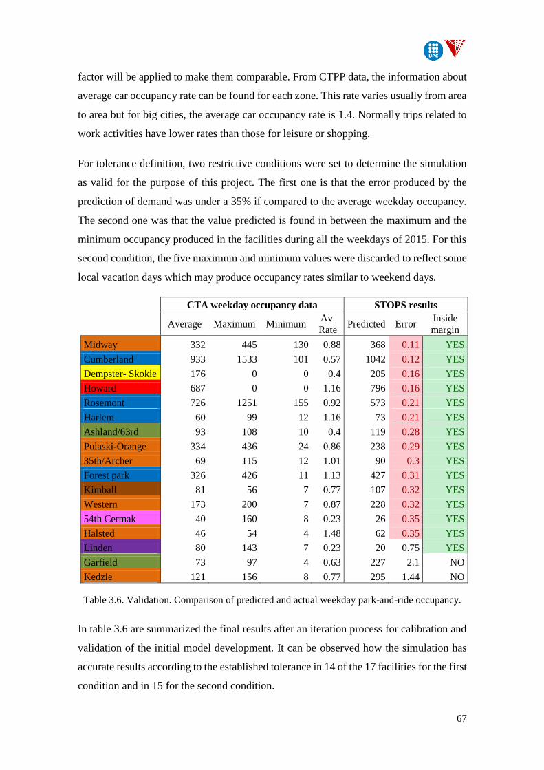
67

factor will be applied to make them comparable. From CTPP data, the information about

average car occupancy rate can be found for each zone. This rate varies usually from area

to area but for big cities, the average car occupancy rate is 1.4. Normally trips related to

work activities have lower rates than those for leisure or shopping.

For tolerance definition, two restrictive conditions were set to determine the simulation

as valid for the purpose of this project. The first one is that the error produced by the

prediction of demand was under a 35% if compared to the average weekday occupancy.

The second one was that the value predicted is found in between the maximum and the

minimum occupancy produced in the facilities during all the weekdays of 2015. For this

second condition, the five maximum and minimum values were discarded to reflect some

local vacation days which may produce occupancy rates similar to weekend days.

CTA weekday occupancy data STOPS results

Average Maximum Minimum

Av.

Rate Predicted Error

Inside

margin

Midway 332 445 130 0.88 368 0.11 YES

Cumberland 933 1533 101 0.57 1042 0.12 YES

Dempster- Skokie 176 0 0 0.4 205 0.16 YES

Howard 687 0 0 1.16 796 0.16 YES

Rosemont 726 1251 155 0.92 573 0.21 YES

Harlem 60 99 12 1.16 73 0.21 YES

Ashland/63rd 93 108 10 0.4 119 0.28 YES

Pulaski-Orange 334 436 24 0.86 238 0.29 YES

35th/Archer 69 115 12 1.01 90 0.3 YES

Forest park 326 426 11 1.13 427 0.31 YES

Kimball 81 56 7 0.77 107 0.32 YES

Western 173 200 7 0.87 228 0.32 YES

54th Cermak 40 160 8 0.23 26 0.35 YES

Halsted 46 54 4 1.48 62 0.35 YES

Linden 80 143 7 0.23 20 0.75 YES

Garfield 73 97 4 0.63 227 2.1 NO

Kedzie 121 156 8 0.77 295 1.44 NO

Table 3.6. Validation. Comparison of predicted and actual weekday park-and-ride occupancy.

In table 3.6 are summarized the final results after an iteration process for calibration and

validation of the initial model development. It can be observed how the simulation has

accurate results according to the established tolerance in 14 of the 17 facilities for the first

condition and in 15 for the second condition.

68

In fact, the iteration process was quite straightforward since the initial model was already

calibrated by RTA. There are two of the facilities which do not fulfill neither of the two

conditions. These are Garfield and Kedzie park-and-rides. It has been considered that

modifying the model only for these two facilities will alter the good matching for the

other stations. For this reason, the model is maintained for this two, expecting that price

sensitivity will not be affected when increasing rates in posterior sections.

3.4 Results for Park-and-Ride elasticities

Once the model is calibrated and validated for 2015, it can be used to perform a sensibility

analysis of park-and-ride monetary cost variation to observe how price sensitive are each

of them in relation to demand.

Three different simulations are run to obtain results of direct and cross elasticities. The

first one is the simulation without any increase in price (Scenario 0%), which is the base

scenario. The other two represents an increment of a 5% and a 10% of the real price

(Scenario 5% and Scenario 10%).

The concept of elasticity was defined as the percentage change in consumption resulting

from a 1 percent change in price, all else held constant. An average value from both last

scenarios will be calculated to represent the mid-point of the demand curve.

It is very important to take into account the limitations of STOPS at the time of treating

results. STOPS presents the outputs in a series of tables which show demand grouped by

different criteria: districts-to-districts, by station or by routes. Many of the tables are also

cross-classified by trip purpose and mode of access.

Demand at each park-and-ride facility can be extracted from results for each station

group. Then, for each of them it can be calculated the direct elasticity when comparing

results from the base scenario with scenario 5% and scenario 10%.

For cross elasticities, the analysis of the impact is not as straightforward as for direct

elasticities. The objective is to determine the effect of the increase of price in other modes.

However, the impact might not be localized in one station or route. This is the reason why

cross-elasticities are calculated by districts, obtaining a representative value for the

impact of one or several park-and-ride facilities with similar transportation patterns. The

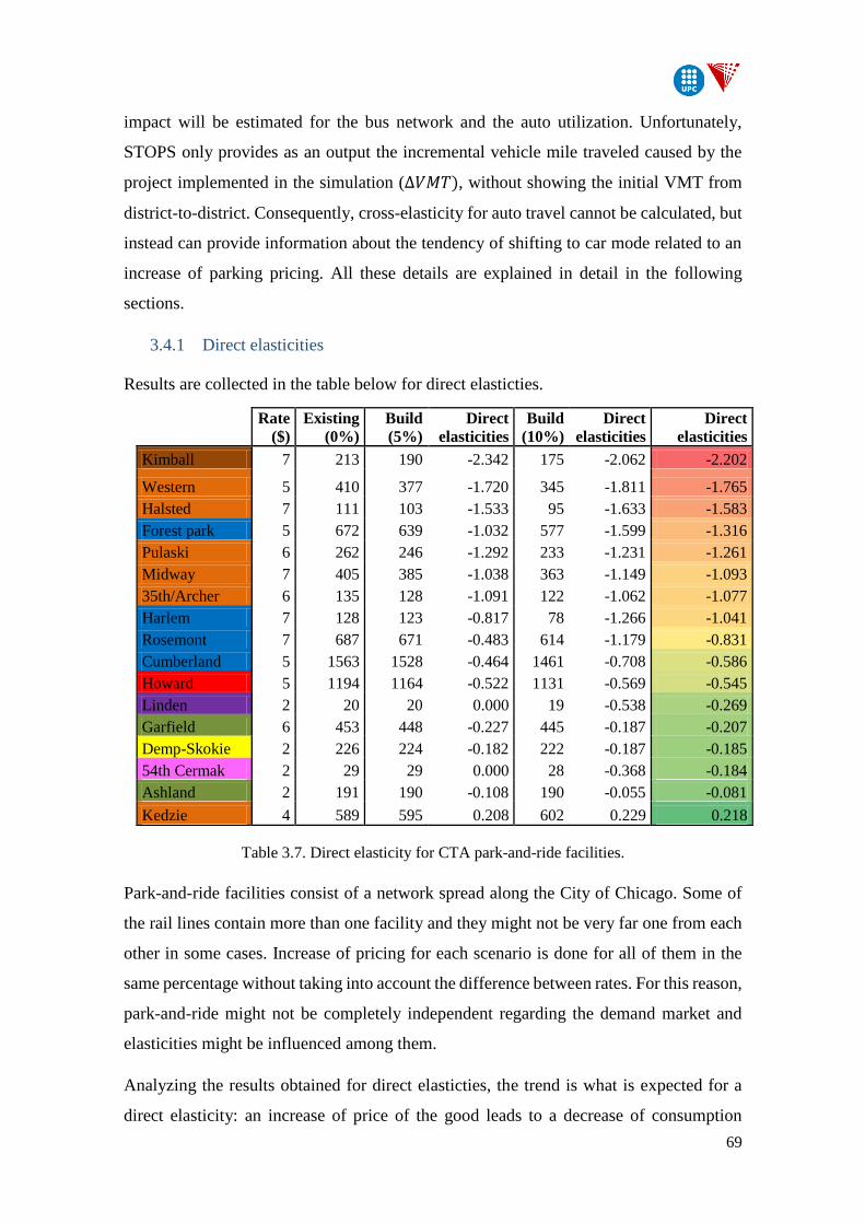
69

impact will be estimated for the bus network and the auto utilization. Unfortunately,

STOPS only provides as an output the incremental vehicle mile traveled caused by the

project implemented in the simulation (∆𝑉𝑀𝑇), without showing the initial VMT from

district-to-district. Consequently, cross-elasticity for auto travel cannot be calculated, but

instead can provide information about the tendency of shifting to car mode related to an

increase of parking pricing. All these details are explained in detail in the following

sections.

3.4.1 Direct elasticities

Results are collected in the table below for direct elasticties.

Rate

($)

Existing

(0%)

Build

(5%)

Direct

elasticities

Build

(10%)

Direct

elasticities

Direct

elasticities

Kimball 7 213 190 -2.342 175 -2.062 -2.202

Western 5 410 377 -1.720 345 -1.811 -1.765

Halsted 7 111 103 -1.533 95 -1.633 -1.583

Forest park 5 672 639 -1.032 577 -1.599 -1.316

Pulaski 6 262 246 -1.292 233 -1.231 -1.261

Midway 7 405 385 -1.038 363 -1.149 -1.093

35th/Archer 6 135 128 -1.091 122 -1.062 -1.077

Harlem 7 128 123 -0.817 78 -1.266 -1.041

Rosemont 7 687 671 -0.483 614 -1.179 -0.831

Cumberland 5 1563 1528 -0.464 1461 -0.708 -0.586

Howard 5 1194 1164 -0.522 1131 -0.569 -0.545

Linden 2 20 20 0.000 19 -0.538 -0.269

Garfield 6 453 448 -0.227 445 -0.187 -0.207

Demp-Skokie 2 226 224 -0.182 222 -0.187 -0.185

54th Cermak 2 29 29 0.000 28 -0.368 -0.184

Ashland 2 191 190 -0.108 190 -0.055 -0.081

Kedzie 4 589 595 0.208 602 0.229 0.218

Table 3.7. Direct elasticity for CTA park-and-ride facilities.

Park-and-ride facilities consist of a network spread along the City of Chicago. Some of

the rail lines contain more than one facility and they might not be very far one from each

other in some cases. Increase of pricing for each scenario is done for all of them in the

same percentage without taking into account the difference between rates. For this reason,

park-and-ride might not be completely independent regarding the demand market and

elasticities might be influenced among them.

Analyzing the results obtained for direct elasticties, the trend is what is expected for a

direct elasticity: an increase of price of the good leads to a decrease of consumption

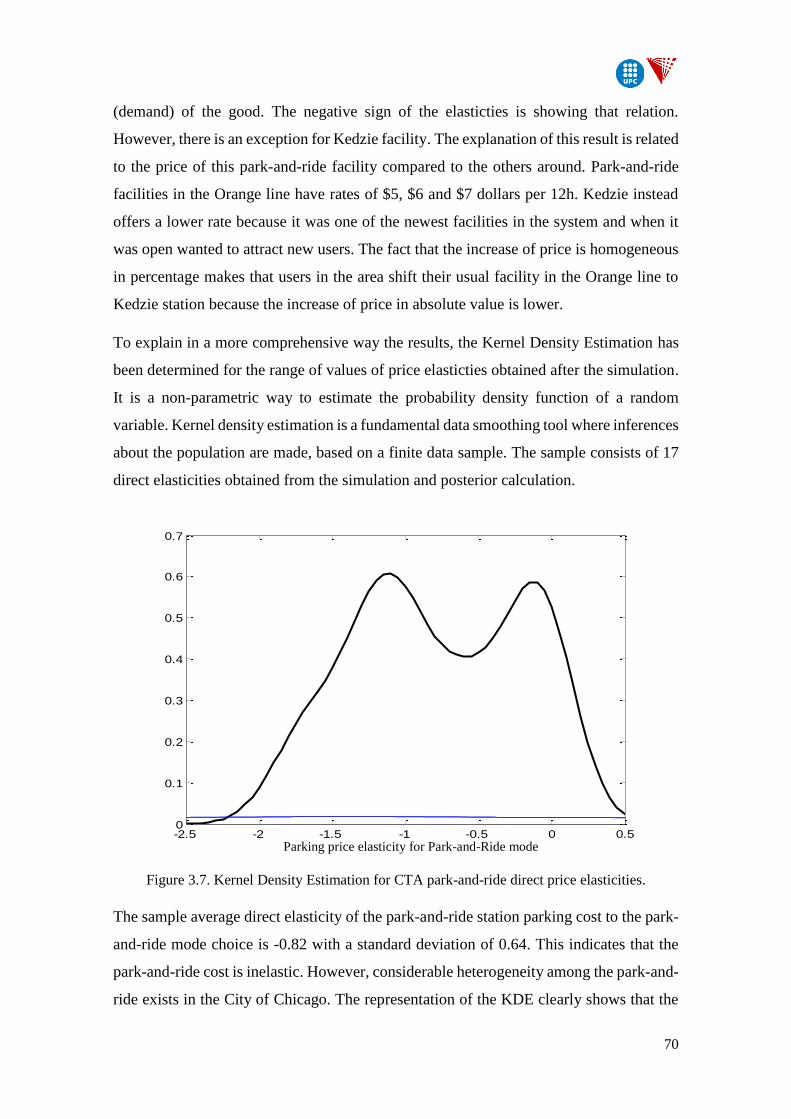
70

(demand) of the good. The negative sign of the elasticties is showing that relation.

However, there is an exception for Kedzie facility. The explanation of this result is related

to the price of this park-and-ride facility compared to the others around. Park-and-ride

facilities in the Orange line have rates of $5, $6 and $7 dollars per 12h. Kedzie instead

offers a lower rate because it was one of the newest facilities in the system and when it

was open wanted to attract new users. The fact that the increase of price is homogeneous

in percentage makes that users in the area shift their usual facility in the Orange line to

Kedzie station because the increase of price in absolute value is lower.

To explain in a more comprehensive way the results, the Kernel Density Estimation has

been determined for the range of values of price elasticties obtained after the simulation.

It is a non-parametric way to estimate the probability density function of a random

variable. Kernel density estimation is a fundamental data smoothing tool where inferences

about the population are made, based on a finite data sample. The sample consists of 17

direct elasticities obtained from the simulation and posterior calculation.

Figure 3.7. Kernel Density Estimation for CTA park-and-ride direct price elasticities.

The sample average direct elasticity of the park-and-ride station parking cost to the park-

and-ride mode choice is -0.82 with a standard deviation of 0.64. This indicates that the

park-and-ride cost is inelastic. However, considerable heterogeneity among the park-and-

ride exists in the City of Chicago. The representation of the KDE clearly shows that the

-2.5 -2 -1.5 -1 -0.5 0 0.50

0.1

0.2

0.3

0.4

0.5

0.6

0.7

Parking price elasticity for Park-and-Ride mode

71

direct elasticity has a bi-modal distribution with one modal value clearly elastic and the

other clearly inelastic. It indicates that two different kind of users in different parts of the

city respond to different way to price change. In the next section of this chapter it is

performed a spatial analysis to identify which are the land and socioeconomic variables

which conform the environment of park-and-ride areas and to relate them with the

elasticities obtained.

To add reliability to this study, direct elasticities obtained from the simulation using

STOPS are contrasted with other related studies on the same field. In 2014, K. N. Habib,

M. S. Mahmoud and J. Coleman from the University of Toronto published an article

making reference to price elasticities in park-and-ride facilities in the Greater Vancouver

Region. They performed a Stated Preference (SP) survey-based study on commuters’

willingness to pay for parking at 14 park-and-ride transit stations. The resulting data was

used to model mode choice for commuter trips and determine parking price elasticities.

The Kernel Density Estimation was plotted for the direct elasticities obtained from their

model evaluated at the 14 park-and-ride station and the results are showed in the figure

below.

Figure 3.8. KDE for Greater Vancouver Region (GVR) park-and-ride direct price elasticities. K.

N. Habib, M. S. Mahmoud and J. Coleman (2014)

72

The sample average direct elasticity for the Greater Vancouver Region for park-and-ride

facilities was -0.94 with a standard deviation of 0.34. It is very interesting to observe that

the range of values for direct elasticities are very similar, showing a bi-modal distribution

in both cases: one elastic and the other inelastic. The average direct elasticity is

considerably close. In contrast, standard deviation for Chicago Area is double the one for

the Vancouver Region study. The explanation for this phenomenon is related to the

context of the city. Chicago is one of the city within US with higher socioeconomic

contrasts from district to district, and instead, Vancouver shows a relatively homogeneous

population characteristics across the region.

3.4.2 Cross-elasticities

Park-and-ride price change, as indicated by the results of previous part cause a decrease

in the demand of park-and-ride facilities. However, this does not mean that users stop

doing their trips. Those users who were accessing transit with car, now might shift to

other modes to access or even to do their whole trip only with one transit mode or with

car.

Cross-elasticities are a good index to determine if the increase of price will have a good

or a bad repercussion on the urban transportation system. As park-and-ride are defined as

transit-oriented facilities, the idea is that they promote the utilization of public

transportation systems. A positive impact of increased charges would be moving users

from private to public modes of mobility. If, on the other hand, users tend to shift to car

as unique mode towards their destination, highways will be congested and will it will lead

to increase the cost for the society.

In this part, it is estimated the impact on the bus network as complementary mode to rail

system. It is also analyzed the incremental vehicle-miles travelled by users due to the

increase of parking rates. At the beginning of this section it is commented that cross-

elasticities are defined by districts and not by park-and-ride stations.

Bus + rail combination:

In the following table, results are presented for cross-elasticities for users traveling with

a combination of bus and rail to their destination. The sample of people used to calculate

the impact of the increased parking rates are the total users who combine these two modes.

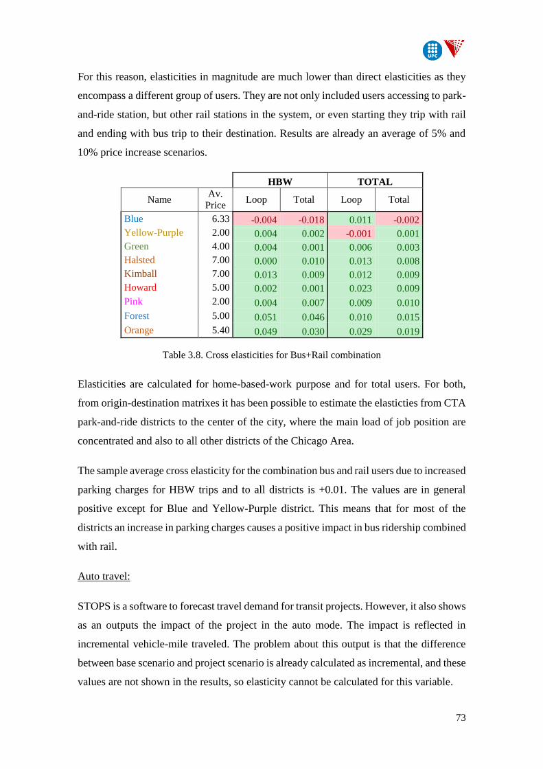
73

For this reason, elasticities in magnitude are much lower than direct elasticities as they

encompass a different group of users. They are not only included users accessing to park-

and-ride station, but other rail stations in the system, or even starting they trip with rail

and ending with bus trip to their destination. Results are already an average of 5% and

10% price increase scenarios.

HBW TOTAL

Name Av.

Price Loop Total Loop Total

Blue 6.33 -0.004 -0.018 0.011 -0.002

Yellow-Purple 2.00 0.004 0.002 -0.001 0.001

Green 4.00 0.004 0.001 0.006 0.003

Halsted 7.00 0.000 0.010 0.013 0.008

Kimball 7.00 0.013 0.009 0.012 0.009

Howard 5.00 0.002 0.001 0.023 0.009

Pink 2.00 0.004 0.007 0.009 0.010

Forest 5.00 0.051 0.046 0.010 0.015

Orange 5.40 0.049 0.030 0.029 0.019

Table 3.8. Cross elasticities for Bus+Rail combination

Elasticities are calculated for home-based-work purpose and for total users. For both,

from origin-destination matrixes it has been possible to estimate the elasticties from CTA

park-and-ride districts to the center of the city, where the main load of job position are

concentrated and also to all other districts of the Chicago Area.

The sample average cross elasticity for the combination bus and rail users due to increased

parking charges for HBW trips and to all districts is +0.01. The values are in general

positive except for Blue and Yellow-Purple district. This means that for most of the

districts an increase in parking charges causes a positive impact in bus ridership combined

with rail.

Auto travel:

STOPS is a software to forecast travel demand for transit projects. However, it also shows

as an outputs the impact of the project in the auto mode. The impact is reflected in

incremental vehicle-mile traveled. The problem about this output is that the difference

between base scenario and project scenario is already calculated as incremental, and these

values are not shown in the results, so elasticity cannot be calculated for this variable.

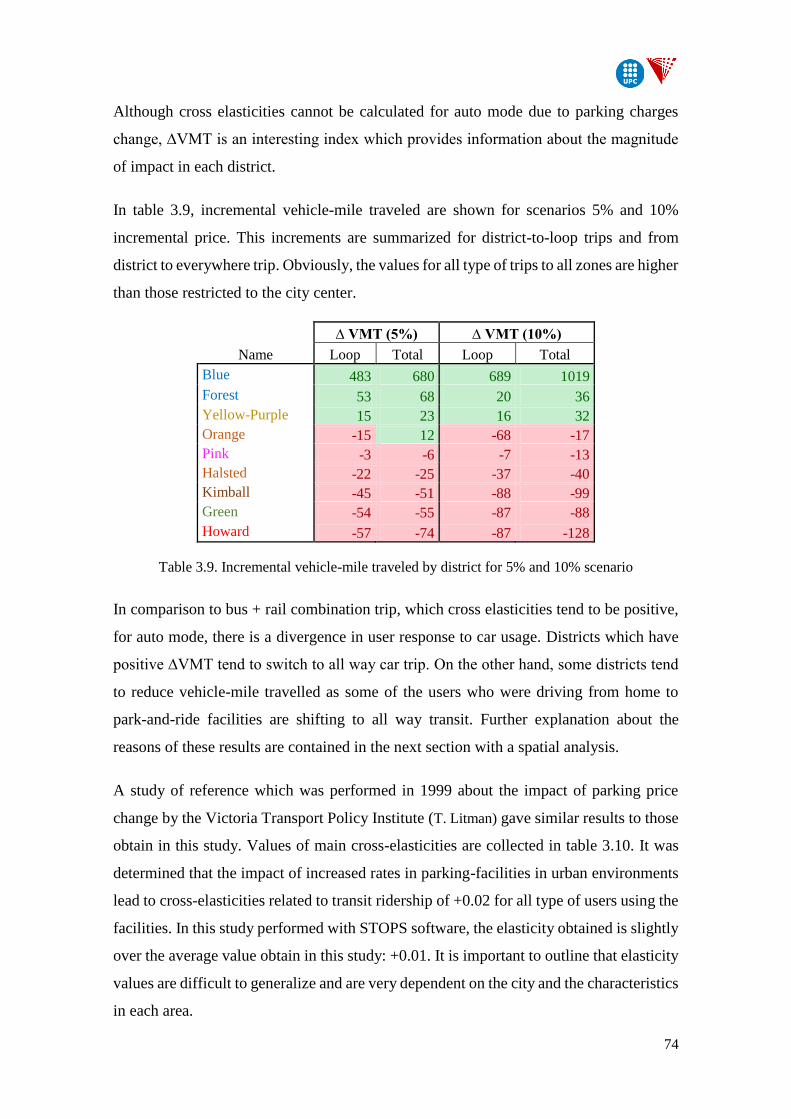
74

Although cross elasticities cannot be calculated for auto mode due to parking charges

change, ∆VMT is an interesting index which provides information about the magnitude

of impact in each district.

In table 3.9, incremental vehicle-mile traveled are shown for scenarios 5% and 10%

incremental price. This increments are summarized for district-to-loop trips and from

district to everywhere trip. Obviously, the values for all type of trips to all zones are higher

than those restricted to the city center.

∆ VMT (5%) ∆ VMT (10%)

Name Loop Total Loop Total

Blue 483 680 689 1019

Forest 53 68 20 36

Yellow-Purple 15 23 16 32

Orange -15 12 -68 -17

Pink -3 -6 -7 -13

Halsted -22 -25 -37 -40

Kimball -45 -51 -88 -99

Green -54 -55 -87 -88

Howard -57 -74 -87 -128

Table 3.9. Incremental vehicle-mile traveled by district for 5% and 10% scenario

In comparison to bus + rail combination trip, which cross elasticities tend to be positive,

for auto mode, there is a divergence in user response to car usage. Districts which have

positive ∆VMT tend to switch to all way car trip. On the other hand, some districts tend

to reduce vehicle-mile travelled as some of the users who were driving from home to

park-and-ride facilities are shifting to all way transit. Further explanation about the

reasons of these results are contained in the next section with a spatial analysis.

A study of reference which was performed in 1999 about the impact of parking price

change by the Victoria Transport Policy Institute (T. Litman) gave similar results to those

obtain in this study. Values of main cross-elasticities are collected in table 3.10. It was

determined that the impact of increased rates in parking-facilities in urban environments

lead to cross-elasticities related to transit ridership of +0.02 for all type of users using the

facilities. In this study performed with STOPS software, the elasticity obtained is slightly

over the average value obtain in this study: +0.01. It is important to outline that elasticity

values are difficult to generalize and are very dependent on the city and the characteristics

in each area.

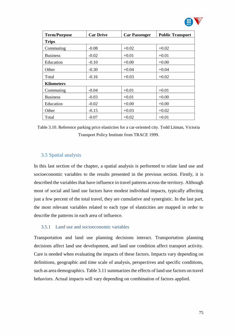
75

Term/Purpose Car Drive Car Passenger Public Transport

Trips

Commuting -0.08 +0.02 +0.02

Business -0.02 +0.01 +0.01

Education -0.10 +0.00 +0.00

Other -0.30 +0.04 +0.04

Total -0.16 +0.03 +0.02

Kilometers

Commuting -0.04 +0.01 +0.01

Business -0.03 +0.01 +0.00

Education -0.02 +0.00 +0.00

Other -0.15 +0.03 +0.02

Total -0.07 +0.02 +0.01

Table 3.10. Reference parking price elasticties for a car-oriented city. Todd Litman, Victoria

Transport Policy Institute from TRACE 1999.

3.5 Spatial analysis

In this last section of the chapter, a spatial analysis is performed to relate land use and

socioeconomic variables to the results presented in the previous section. Firstly, it is

described the variables that have influence in travel patterns across the territory. Although

most of social and land use factors have modest individual impacts, typically affecting

just a few percent of the total travel, they are cumulative and synergistic. In the last part,

the most relevant variables related to each type of elasticities are mapped in order to

describe the patterns in each area of influence.

3.5.1 Land use and socioeconomic variables

Transportation and land use planning decisions interact. Transportation planning

decisions affect land use development, and land use condition affect transport activity.

Care is needed when evaluating the impacts of these factors. Impacts vary depending on

definitions, geographic and time scale of analysis, perspectives and specific conditions,

such as area demographics. Table 3.11 summarizes the effects of land use factors on travel

behaviors. Actual impacts will vary depending on combination of factors applied.

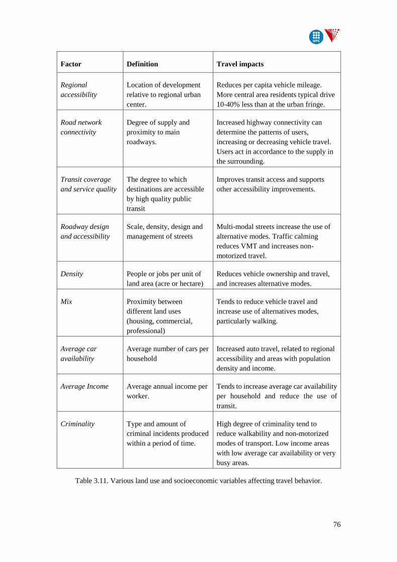
76

Factor Definition Travel impacts

Regional

accessibility

Location of development

relative to regional urban

center.

Reduces per capita vehicle mileage.

More central area residents typical drive

10-40% less than at the urban fringe.

Road network

connectivity

Degree of supply and

proximity to main

roadways.

Increased highway connectivity can

determine the patterns of users,

increasing or decreasing vehicle travel.

Users act in accordance to the supply in

the surrounding.

Transit coverage

and service quality

The degree to which

destinations are accessible

by high quality public

transit

Improves transit access and supports

other accessibility improvements.

Roadway design

and accessibility

Scale, density, design and

management of streets

Multi-modal streets increase the use of

alternative modes. Traffic calming

reduces VMT and increases non-

motorized travel.

Density People or jobs per unit of

land area (acre or hectare)

Reduces vehicle ownership and travel,

and increases alternative modes.

Mix Proximity between

different land uses

(housing, commercial,

professional)

Tends to reduce vehicle travel and

increase use of alternatives modes,

particularly walking.

Average car

availability

Average number of cars per

household

Increased auto travel, related to regional

accessibility and areas with population

density and income.

Average Income Average annual income per

worker.

Tends to increase average car availability

per household and reduce the use of

transit.

Criminality Type and amount of

criminal incidents produced

within a period of time.

High degree of criminality tend to

reduce walkability and non-motorized

modes of transport. Low income areas

with low average car availability or very

busy areas.

Table 3.11. Various land use and socioeconomic variables affecting travel behavior.

77

3.5.2 Spatial analysis

The spatial structure of cities, in developing countries particularly, is highly contrasted.

In some areas services and facilities are adequately provided while there are inadequate

or no services provided in others. Similarly there is a variation in socio-economic

characteristic of the dwellers from place to place. These variations bring the challenge of

getting equal and efficient urban services for all the citizens. Quality of life is closely

related to people accessibility to alternative employment, educational and medical

facilities, essential public services, and nature or extensive recreational open space.

Due to all these complex parameters that conform the territory, pricing policies in

transportation systems can affect in a different way from place to place. The objective of

this last part of the chapter is define the relations between parking price sensitivity and

the characteristic of the area of influence.

All the previous land and socioeconomic variables are calculated for each TRACT zone,

extracting data from different sources, such as community surveys, open data from the

online Chicago Data Portal, where information is provided in tables and shapefiles. Data

have been grouped according to TRACT belonging to same districts to obtain averaged

indexes which reflects their principal characteristics. ESRI 2011. ArcGIS Desktop

(Release 10), has been used as a tool to combine all these files and perform a visual and

descriptive analysis.

Direct elasticity:

Park and ride facilities allow commuters to avoid a stressful drive along congested roads

and a search for scarce, expensive city-center parking. Users having the decision of using

park-and-ride facilities want to find an equilibrium between travel time and parking cost.

The closer to the center the more expensive the parking rate, but the shortest the transit

trip till their destination. It consists on a trade of between cost impedances in time or

distance to the main activity center (regional accessibility) and the monetary cost

associated to the facility.

If time costs are maintained as a constant for transit riders independently of the degree of

ridership, an increase of price of parking charges will produce a decrease in number of

users, especially in those facilities where rates are already high compared to the others

nearby.

78

In figure 3.9 the price sensitivity is illustrated through direct elasticities at all the CTA

park-and-ride stations by colored dots at their locations. They are also included main road

and bus network plotted in the area of influence of the 17 park-and-ride facilities in a 3

mile radius which is the catchment area defined by STOPS. As mentioned before, user

decisions are based on the distance and the time to the main activity centers. For this

reason, TRACTS are colored according to job density and labeled areas have been defined

from the area where we find higher work trip attraction and mix in relation to

office/residence ratio, which in this case is the downtown area: The Loop.

Two main clusters are created by the intersection of the areas of influence of the 17 CTA

park-and-ride:

- For the northern cluster, the closest facility to downtown is located inside the

second ring, where job attraction is shown to be important. It is Kimball Park-and-

Ride for the Brown line. The parking rate is the highest of all the facilities located

in the cluster: 7$ per 12 hours. This facility is presenting an inelastic response to

increased charges, which means that the amount of users drops at a high rate in

relation to the increment of demand. The explanation of this, attending to regional

accessibility, is that users who still want to use car as an access mode, coming

from the Metropolitan Area of Chicago, have other park-and-ride options in the

third ring, which may increase in-vehicle travel time for transit but reduce

considerably the monetary cost of using the lots. As observed in the figure,

facilities in the third ring of the cluster have all a lower and elastic response to

price change. Values are comprised between -0.9 and -0.6 for Blue line facilities,

and from -0.6 to -0.1 in the bifurcation system Red-Yellow-Purple facilities.

- For the southern cluster, results are more disperse. However, there is still the trend

of having inelastic responses in the facilities closer to downtown. Both Halsted

and 35th/Archer facilities located inside the first ring, present direct elasticities

over 1.00 in absolute value. They are also two of the facilities with higher pricing

rates in the southern cluster: 7 and 6 dollars per 12 hours respectively. Inside the

second ring we find divergence in the user’s response. As a general trend, orange

line presents a inelastic response and the other lines, in particular Green and Pink

line present elastic elasticities, which locate the facilities at the end of the line.

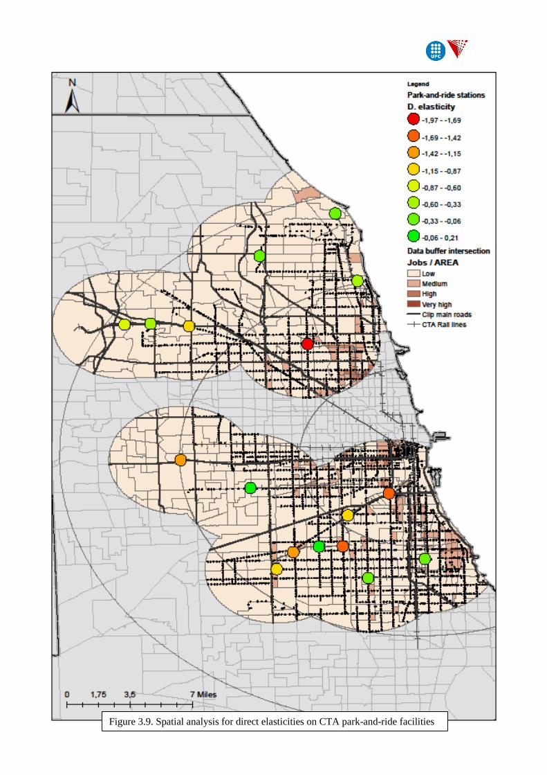
79

Figure 3.9. Spatial analysis for direct elasticities on CTA park-and-ride facilities

80

Cross elasticities and ∆VMT:

Figures 3.10 and 3.11 show the impact of the implemented project in users shifting mode

of transportation when doing their trips. Both are really related as normally modes are

complementary and all modes supply support the total demand of the system.

Figure 3.10 shows the cross elasticities of parking price increase for users shifting to bus

to get access to rail towards their destination. Data about criminality in public

transportation environment is included in the mapping as a representative variable that

affects to users choices when getting access to a rail station.

Figure 3.11 illustrates with colored dots the impact of increased pricing in park-and-ride

facilities on the incremental vehicle-mile traveled in the districts that allocate these

stations. Tracts are also colored according to average vehicle availability per household.

This variable is in fact an index of wealth, directly related to the average income in the

region.

For both of the figures, main roads and bus stations are plotted to show the coverage of

these modes throughout the area of influence.

Big negative impact on the transportation network due to increase in parking charges is

spotted in those lots associated to the Blue, Purple and Yellow line. They are all located

in the third ring of the northern cluster. Figure 3.11 shows how users in that region tend

to switch to auto travel instead of relying on public transportation to reach their

destinations. Cross elasticities for transit access to rail station are negative for the facilities

in the Blue line. Park-and-ride facilities are a connection between the road and the transit

system. Although normally users who park in the facility shift to rail, some of them might

shift to bus to get to their destinations. For Linden and Dempster-Skokie facilities, they

present cross elasticities very close to zero. On the other hand, ∆VMT is positive in these

districts, meaning that users have a clear preference for the private mode. This can be

explain according to the following points:

- Transit service and coverage, especially for the bus network is poor in this sector

compared to other areas in the city. People have less accessibility to transit as a

mode of access to the principal CTA rail stations.

81

- Population density is lower in that area, which means that the neighborhoods are

more residential and the street grid is less dense. Normally grid density provides

agglomeration efficiencies and increase of public transit service efficiency.

- Average vehicle availability is 1.5 for users in the area of influence of Blue line

facilities and 1.65 for the northern part of the cluster. This is strictly related to

income. Higher incomes are living in the north part of the city and close to the

Lake Michigan.

- Park-and-ride facilities in this sector are the furthest of the system. The greater the

distance to major activity centers, the higher the tendency of using car.

- Main road network connectivity to park-and-ride facilities is high. Particularly for

the Blue line, where the CTA stations are located in between the lanes of the

highway and parking facilities are on one of the sides. High connectivity is

positive to facilitate access to the facility, but on the other hand, consists on an

immediate alternative for users if there is an increase of price of the facilities.

For the other park-and-ride facilities located within the second and the first ring, the

tendency of the users is inverted. Incremental vehicle mile travel is negative, and cross-

elasticities for bus plus rail ridership is positive, which means that users tend to shift to

public transportation systems, if there is an increase in park-and-ride rates.

- Opposite to the previous described region, these two rings present higher

population density as they are closer to main services and job attraction areas.

- Any type of density causes an agglomeration of activity and therefore the

existence of transportation system supply, more oriented to transit, as public

transportation system has economies of scale.

- Grid density is higher, improving pedestrian and bicycle travel, and therefore

public transit access and encourages more local activities.

- Criminality is taking an important role in users decisions. Southside of Chicago

(Green line) and west part have high indexes of criminality in public

transportation system like in public stations and inside the vehicle. Although these

areas are the poorest of the region and car availability rate is the lowest too,

commuters who work in downtown still prefer take the car from home to the rail

station and avoid exposure to crime.

82

Figure 3.10. Spatial analysis for cross elasticities on CTA park-and-ride facilities

83

Figure 3.11. Spatial analysis for ∆VMT in the area of influence of CTA park-and-ride facilities

84

C

HA

PTE

R 4

SUMMARY AND

CONCLUSION

85

4. SUMMARY AND CONCLUSION.

4.1 Summary

Park-and-ride facilities are meant to encourage drivers to park their cars some distance

away from the city center and complete their journey by public transport. However, user

decision of accessing transit by car depends on their perceived cost in relation to other

possible options presented in the urban environment. User costs include monetary costs,

travel time, discomfort and risk. Pricing impacts are used in this thesis to measure

elasticities: the percentage change in demand that results from each 1% change in price.

The determination and evaluation of price elasticities for park-and-ride facilities

associated to the CTA “L” rail line has been the main objective of this study. As explained

in chapter 2, this is a very new study for the city of Chicago, as park-and-ride elasticities

have never been determined before by any other study and they provide a useful

information to the operator to manage and apply specific strategies for the exploitation of

the facilities after accurate analysis.

STOPS has been the principal tool to perform the prediction of demand at the facilities

and within the system in relation to a price change in real parking cost rates for 17 CTA

stations. STOPS is a software that was released in 2013 by the Federal Transit

Administration to motivate public and private institutions to implement transit project

seeking for a social benefit in urban systems across the US. The models implemented in

this software to develop travel demand forecasting have been described in chapter 3, to

have criteria at the time of analyzing the outputs, outlining its capabilities and limitations.

In chapter 4, the procedure to perform the price sensitivity study at the 17 park-and-ride

facilities for the City of Chicago has been detailed.

In a first phase, inputs for STOPS, released by the Regional Transit Authority of Chicago,

after a calibration and validation process, have been described and particularized for this

study. These include socioeconomic data, transportation network definition and

demographics.

Secondly, a model to implement a penalization cost accounting for park-and-ride rates

and characteristics, has been presented. This model has been calibrated and validated after

86

treatment of real data provided by the Chicago Transit Authority about the occupancy

rates of each facility during 2015.

Once, the model is calibrated and validated, a sensibility analysis has been performed

through several pricing scenarios simulated with STOPS to forecast the demands in the

system in relation to price variation.

Direct and cross elasticities have been estimated taking into account STOPS output

limitations and have been compared to reference studies about park-and-ride price

elasticities published in the last years.

Finally, a spatial analysis has been performed using GIS tools in relation to main land use

and socioeconomic variables. The objective of this analysis has been to find relations

between the urban and social configuration of the city of Chicago and the price sensitivity

of users to parking rates in each area. A further insight in preferred mode alternatives for

users due to parking price increase has been done.

4.2 Findings

STOPS software:

STOPS has been proved to be a useful tool to predict travel demand volumes, which is

well calibrated and validated to represent existing and future scenarios in different urban

environments. However, it still presents some limitations regarding criteria for model

development and presentation of outputs:

STOPS estimates transit demand that is not constrained by transit systems and

capacity.

STOPS considers routine weekday trips by residents but is not taking into

account special travel markets such air passengers, students or visitors.

Fortunately, this has little influence in the type of user of park-and-ride

facilities.

STOPS uses the zone-to-zone roadway travel times and distances from the

regional travel model developed by CMAP which are not modified according

to the variation of vehicle-mile traveled as a consequence to project

implementation.

87

STOPS outputs are limited to several series of tables which show predicted

demand classified by district-to-district, routes or stations. Those are cross-

classified by trip purpose and mode of access to transit system. Limited access

modes makes complex to perform impact analysis on other ways to reach

destination as combination of modes in urban trips.

Price elasticities:

Regarding direct elasticities obtained for the CTA park-and-ride system, they show to

have a bimodal distribution with a set of elastic and a set of inelastic elasticity groups

with an average value of the sample of -0.82. Results are comprised in a range of values

very similar to those obtained for a study performed in 2013 for the Vancouver Greater

Area, using a different methodology for user mode choice.

Further spatial analysis leads to the general conclusion that user’s choice of accessing to

a specific park-and-ride and shiftting to transit is a tradeoff between the location of the

facility relative to the main activity center of the city and the parking rate. Users try to

minimize the monetary cost and in-vehicle travel time in the system. But both of them

have inverse relation, the nearer the facility to downtown, the lower the transit travel time

and the higher the rates. For this reason, an increase of price in parking rates cause

inelastic response in those facilities which are nearer to downtown where the demands

drop at a higher rate due to the fact that other facilities with lower prices are located in

stops more external areas of the city.

Regarding impacts on the transportation network (bus and road system), cross elasticities

and incremental vehicle mile traveled have shown to have a strong relationship in the

response of users as bus, car and rail are complementary modes. Cross elasticities showed

to be positive in average with an impact of +0.01, which means that increased price

charges lead in general to a higher transit ridership. However there are areas of the city

where the trend is the inverse. Users preferred shifting to all-way car trips to get to their

destination instead of using public transit systems.

Spatial analysis indicated how these results were strictly associated mainly to three

factors:

- Socioeconomic conditions. Neighborhoods with higher incomes and higher

average vehicle availability index showed to be pro-auto.

88

- Population, services and urbanization density are strictly related, and they lead to

higher degree of accessibility, promoting transit utilization, and are related to

those areas with positive cross-elasticities and a reduction in auto travel.

- Bus and road connectivity. The type of transportation system coverage determines

different choices that users have in their surroundings and consequently the travel

patter in the area. Park-and-ride facilities nearer to highways present higher

shifting rates to auto due to increased price. On the opposite, areas with higher

bus coverage, which at the same time are those with higher density and lower

accessibility to road network, present a higher shifting rate to bus as an access

mode.

4.3 Future lines of research

This thesis has reviewed the most relevant studies about park-and-ride price elasticties

that have been published during the last years and have provided with new information

about the characteristics of travel decision and behavior of users within the Chicago Area.

Managing commuter parking facilities is a complex endeavor. Considering the cost-

effectiveness of pricing, the goal of parking management intended to create livable

communities. Park-and-ride price elasticities are useful parameters to address pricing

policies which maximize the benefits of the operators and the society. For this reason, the

results obtained in this thesis are key parameters to define spatial strategies to achieve

these goals.

Future research has to focus on the utilization of these parameters to improve the system

performance, which means finding an equilibrate parking pricing supply that attracts

greater demand where increased charges may have negative externalities and, at the same

time, try to promote transit systems in areas where users tend to shift easily to these kind

of modes by increasing rates.

89

90

REFERENCES

A. M. Lago, P. Mayworm and J. M. McEnroe, 1981 Transit Service Elasticities. Journal

of Transport Economics and Policy, Vol. X, No X.

Ben-Akiva, M. E. and S. R. Lerman, 1985. Discrete Choice Analysis: Theory and

Application to Travel Demand, MIT, Massachusetts, US

Cambridge Systematics, Inc.; Vanasse Hangen Brustlin, Inc.; Gallop Corporation;

Chandra R. Bhat; Shapiro Transportation Consulting, LLC and

Martin/Alexiou/Bryson, PLLC, 2012. Travel Demand Forecasting: Parameters and

Techniques. Transportation Research Board. NCHRP Report 716.

Cambridge Systematic, Inc, 2015. Review of Transit Modeling with Respect to Federal

Transit Administration Guidance. Extracted 15-02-17 from https://www.mwcog.org/

ESRI 2011. ArcGIS Desktop: Release 10. Redlands, CA: Environmental Systems

Research Institute.

Fan. K., J. E. Miller and D. Badoe, 1993. Modeling Rail Access Mode and Station Choice.

Transportation Research Record 1213: 49-59

Federal Transit Administration 2013. Simplified Trips-on-Project Software (STOPS).

Version 1.5. Washington, DC. Planning and Environment Department.

Foote, P. J., 2000. Chicago Transit Authority Weekday Park-and-Ride Users: Choice

Market with Ridership Growth Potential. Transportation Research Record: Journal of

the Transportation Research Board 1735(-1): 158-168.

García, R. and A. Marín, 2002. Parking Capacity and Pricing in Park'n Ride Trips: A

Continuous Equilibrium Network Design Problem. Annuals of Operations Research

116(1): 153-178.

Gillespie W, 2015. STOPS for Chicago. Guide to Regionally Calibrated Model Inputs.

Version 1.50rta 1.0. Regional Transportation Authority of Chicago

Jay E. and Xuemei L., 2014. Using the Federal Transit Administration (FTA) Simplified

Trips-on-Project Software (STOPS) for Transit Demand Estimation. 2014 ITE Mid-

Colonial District and Mid-Atlantic Section Annual Meeting. Extracted the 27-02-17

from: http://www.masite.org/.

J.Xie, S. C. Wrong, and S.M. Lo, 2017. Three Extensions of Tong and Richardson’s

Algorithm for Finding the Optimal Path in Schedule-Based Railway Networks.

Journal of Advanced Transportation. Volume 2017. Article ID 0216864

Litman, T. and R. Steele, 2017. Land Use Impact on Transport. How Land Use Factors

Affect Travel Behaviour. Victoria Transport Policy Institute

Litman T, 2004. Transit Price Elasticities and Cross-Elasticities. Victoria Transport

Policy Institute. Journal of Public Transportation, Vol. 7, No 2.

Martin W. A. and Mcgucking N. A, 1998. Travel Estimation Techniques for Urban

Planning. Transportation Research Board. NCHRP Report 365.

91

Olsson, A.L.L., 2003. Factors that influence choice of travel mode in major urban areas:

the attractiveness of park-and-ride. TRITA-INFRA 03-048, ISSN 1651-0216, ISBN

91-7323-048-0. Department of Infrastructure, Kungl Tekniska Hogskolan, Royal

Institute of Technology of Sweden.

RSG Wilson, 2015. User Guide. STOPS: Simplified Trips-on-Project Software. Extracted the

13-02-2017 from https://www.transit.dot.gov/funding/grant-programs/capital-investments/stops

Ruiter E. and McGuckin N., 2007. A Guidebook for Using American Community Survey

Data for Transportation Planning. Transportation Research Board. NCHRP Report

588.

Savage, I and A. Schupp, 1997. Evaluating Transit Subsidies in Chicago. Journal of

Public Transportation. Volume 1997. Article ID 016524

Shirhakmar M. and E. Deakin, 2005. Study of Park-and-Ride Facilities and Their Use in

the San Francisco Bay Area of California. Transportation Research Record: Journal

of the Transportation Research Board 1927(-1): 46-54.

Syed, S., A. Golub and E. Deakin, 2009. Response of Regional Rail Park-and-Ride Users

to Parking Price Changes. Transportation Research Record: Journal of the

Transportation Research Board 2110(-1): 155-162.

Wells, S. S., 2004. Analysis of the Differential Impacts of Transport Modes on Travel

Behaviour in the Greater Toronto Area. Transportation Research. Part A, Policy and

practice 31:84-94

92