Embed Size (px)
Citation preview
T REPORTECHNICALNO. 298
August 2015
MICHAEL ADJEI KLU
DETERMINATION OF A GEOID MODEL FOR GHANA USING THE
STOKES-HELMERT METHOD
DETERMINATION OF A GEOID MODEL
FOR GHANA USING THE STOKES-
HELMERT METHOD
Michael Adjei Klu
Department of Geodesy and Geomatics Engineering
University of New Brunswick
P.O. Box 4400
Fredericton, N.B.
Canada
E3B 5A3
August, 2015
© Michael Adjei Klu, 2015
PREFACE
This technical report is a reproduction of a thesis submitted in partial fulfillment of
the requirements for the degree of Master of Science in Engineering in the Department of
Geodesy and Geomatics Engineering, August 2015. The research was supervised by Dr.
Peter Dare, and funding was provided by the Ministry of Lands & Natural Resources,
Ghana.
As with any copyrighted material, permission to reprint or quote extensively from this
report must be received from the author. The citation to this work should appear as
follows:
Klu, Michael Adjei (2015). Determination of a Geoid Model for Ghana Using the
Stokes-Helmert Method. M.Sc.E. thesis, Department of Geodesy and Geomatics
Engineering Technical Report No. 298, University of New Brunswick,
Fredericton, New Brunswick, Canada, 91 pp.
ii
ABSTRACT
One of the greatest achievements of humankind with regard to positioning is Global
Navigation Satellite System (GNSS). Use of GNSS for surveying has made it possible to
obtain accuracies of the order of 1 ppm or less in relative positioning mode depending on
the software used for processing the data. However, the elevation obtained from GNSS
measurement is relative to an ellipsoid, for example WGS84, and this renders the heights
from GNSS very little practical value to those requiring orthometric heights. Conversion
of geodetic height from GNSS measurements to orthometric height, which is more useful,
will require a geoid model. As a result, the aim of geodesist in the developed countries is
to compute a geoid model to centimeter accuracy. For developing countries, which
include Ghana, their situation will not even allow a geoid model to decimeter accuracy.
In spite of the sparse terrestrial gravity data of variable density distribution and quality,
this thesis set out to model the geoid as accurately as achievable. Computing an accurate
geoid model is very important to Ghana given the wide spread of Global Positioning
System (GPS) in the fields of surveying and mapping, navigation and Geographic
Information System (GIS). The gravimetric geoid model for Ghana developed in this
thesis was computed using the Stoke-Helmert approach which was developed at the
University of New Brunswick (UNB) [Ellmann and Vaníček, 2007]. This method utilizes
a two space approach in solving the associated boundary value problems, including the
real and Helmert’s spaces. The UNB approach combines observed terrestrial gravity data
with long-wavelength gravity information from an Earth Gravity Model (EGM). All the
terrestrial gravity data used in this computation was obtained from the Geological Survey
Department of Ghana, due to difficulties in obtaining data from BGI and GETECH. Since
iii
some parts of Ghana lack terrestrial gravity data coverage, EGM was used to pad those
areas lacking in terrestrial gravity data. For the computation of topographic effects on the
geoid, the Shuttle Radio Topography Mission (SRTM), a Digital Elevation Model (DTM)
generated by NASA and the National Geospatial Intelligence Agency (NGA), was used.
Since the terrain in Ghana is relatively flat, the topographic effect, often a major problem
in geoid computation, is unlikely to be significant. This first gravimetric geoid model for
Ghana was computed on a 1' 1' grid over the computation area bounded by latitudes 4ºN
and 12ºN, and longitudes 4ºW and 2ºE. GPS/ trigonometric levelling heights were used
to validate the results of the computation.
Keywords: Gravimetric geoid, Stokes’s formula, Earth Gravity Model, Topographic
effect, Digital Terrain Model, Boundary value problem, GPS/trigonometric levelling.

iv
DEDICATION
To my late mother, father, brother, sister and all who have supported and sustained me
during my research and writing at the University of New Brunswick.

v
ACKNOWLEDGEMENTS
The feat achieved by this research could not have been possible without the help and
support of the following:
I am highly indebted to Prof Vaníček for his unflinching support throughout my studies at
the University of New Brunswick. His invaluable guidance, advice, patience, critique,
and quest to go the extra mile to maintained research standards are greatly appreciated. I
feel privileged and honored to work under his guidance.
My special thanks go to Dr. Santos for his invaluable intellectual guidance, professional
discussion and advice during my studies at University of New Brunswick.
My profound gratitude goes to Dr. Dare my supervisor for his constructive feedback on
this research and write-up, unflinching support, professional discussions, flexibility and
availability throughout the study period.
Am grateful to Dr. Kingdon for his wonderful assistance and availability for discussions
on many research issues, which cannot be listed here.
Many thanks go to Mr. Michael Sheng for his wonderful assistance with regard to giving
me a firm grounding on the use of the SHGeo software.
I am very thankful to Mr. Faroughi who provided me with all the Matlab programs for
the data processing
I am grateful to Titus Tienaa for his advice and encouragement throughout my studies.
His support and kindness are examples of a dear friend.
I acknowledge the various organizations and their heads who have funded my studies,
especially Dr. Karikari of the Land Administration Project, Dr. Odame of the Lands
Commission, Dr. Ben Quaye of Lands Commission, Mr. Abeka of Land Administration
Project and Mr. Odametey of Survey and Mapping Division of the Lands Commission.

vi
I am very thankful to Mr. Ben Okang and Mr. Opoku of the Geodetic Section of the
Survey and Mapping Division of the Lands Commission for the moral support.
Last but not the least, am grateful to all my family, friends back in Ghana and Canada
who supported me and made my stay in Canada a memorable one.
Above all I will like to thank Jehovah the God I serve and worship for bringing me this
far and helping me throughout my studies. May your name Jehovah be praised forever.
All I can say is thank you very much.
vii
Table of Contents
ABSTRACT ................................................................................................................... ii
DEDICATION .............................................................................................................. iv
ACKNOWLEDGEMENTS .............................................................................................v
Table of Contents ......................................................................................................... vii
List of Tables...................................................................................................................x
List of Figures ............................................................................................................... xi
List of Symbols, Nomenclature or Abbreviations .......................................................... xii
Chapter 1. Introduction ................................................................................................1 1.1 Description of chapters ..................................................................................................... 1
1.2 Background ....................................................................................................................... 3
1.3 The geoid .......................................................................................................................... 6
1.4 Uses of a geoid model ....................................................................................................... 8
1.5 Research objective and contribution ................................................................................. 9
Chapter 2. Literature review ...................................................................................... 11 2.1 Introduction .................................................................................................................... 11
2.2 The goal for centimeter geoid.......................................................................................... 12
2.3 Techniques for geoid computation .................................................................................. 15
2.4 Remove-compute-restore using Stokes-Helmert method of geoid computation .............. 16
2.5 Least Squares Modification Method (LSMS) also called KTH method ............................... 18
Chapter 3. Theoretical background of Stokes-Helmert’s approach to geoid
determination................................................................................................................. 21 3.1 Introduction .................................................................................................................... 21
3.2 Formulation of geodetic boundary-value problem in real space ....................................... 23
3.3 Gravity anomaly .............................................................................................................. 26
3.4 Transformation of gravity anomalies from the real space to Helmert space ..................... 30
3.5 Effect of topographical masses on gravitational attraction............................................... 33
3.6 Direct Topographic Effect (DTE) ....................................................................................... 35
3.7 Direct Atmospheric Effect (DAE) ...................................................................................... 37
3.8 Secondary Indirect topographical Effect (SITE) ................................................................. 38
3.9 Downward continuation of gravity anomalies .................................................................. 38

viii
3.10 Reference Field.............................................................................................................. 39
3.11 Solution of Stokes’s boundary value problem ................................................................ 40
3.12 Transformation from Helmert’s space to real space ....................................................... 42
3.13 Primary Indirect Topographic Effect (PITE) ..................................................................... 43
3.14 Primary Indirect Atmospheric Effect (PIAE) .................................................................... 44
Chapter 4. Data acquisition ........................................................................................ 45 4.1 Introduction .................................................................................................................... 45
4.2 Terrestrial gravity data in Ghana...................................................................................... 48
4.3 Computing the gravity anomalies and residual gravity anomalies .................................... 52
4.4 Statistical test for outliers ................................................................................................ 53
4.5 Transformation from real space to Helmert’s space ......................................................... 54
4.6 Gridding of the residual gravity anomalies ....................................................................... 55
4.7 Digital Elevation Model (DEM) ......................................................................................... 56
4.8 Computation of Direct Topographic Effect (DTE).............................................................. 58
4.9 Direct Atmospheric Effect (DAE) ...................................................................................... 59
4.10 Secondary Indirect Topographic Effect (SITE) ................................................................. 60
4.11 Helmert anomalies on the topography .......................................................................... 60
4.12 Downward continuation ................................................................................................ 61
4.13 Reference Field.............................................................................................................. 64
4.14 Ellipsoidal corrections .................................................................................................... 65
4.15 Computation of the residual co-geoidal heights ............................................................. 67
4.16 Reference Spheroid ....................................................................................................... 69
4.17 Transformation from Helmert’s space to real space ....................................................... 71
4.18 Primary Indirect Topographic Effect (PITE) ..................................................................... 71
4.19 Primary Indirect Atmospheric Effect (PIAE) .................................................................... 72
4.20 Geoid-Ellipsoid separation ............................................................................................. 74
4.21 GNSS/trigonometric-levelling data................................................................................. 76
Chapter 5. Conclusions and recommendation ............................................................ 82 5.1 Conclusion....................................................................................................................... 82
5.2 Limitations of this research ............................................................................................. 84
5.3 Recommendation ............................................................................................................ 85

ix
Chapter 6. References ................................................................................................ 88
Curriculum Vitae

x
List of Tables
Table 1 Agreement of geoid model heights and GNSS/Trigonometric-levelling .......................... 79
Table 2 Agreement of geoid model heights using ±10 mGal criterion and GNSS/Trigonometric-
levelling .................................................................................................................................... 80
xi
List of Figures
Figure 1-1 The surface of the Earth, geoid and ellipsoid Source: [Burkhard, 1985 ........................ 8
Figure 4-1 Gravity observations in Ghana 1957-58 Source: [Davis, 1958 .................................... 47
Figure 4-2 Distribution of observed terrestrial gravity coverage Source of map: Google ............ 51
Figure 4-3 Histogram of residual gravity anomaly data .............................................................. 54
Figure 4-4 Free-air anomalies mGal ........................................................................................... 56
Figure 4-5 Direct Topographic Effect (DTE) in mGal ................................................................... 58
Figure 4-6 Direct Atmospheric Effect (DTE) in mGal ................................................................... 59
Figure 4-7 Secondary Indirect Topographic Effect (SITE) in mGal ............................................... 60
Figure 4-8 Helmert anomalies in mGal ...................................................................................... 61
Figure 4-9 Differences between Helmert anomalies on topography and downward continuation
in mGal ..................................................................................................................................... 63
Figure 4-10 Reference field in mGal .......................................................................................... 65
Figure 4-11 Ellipsoidal correction for gravity in mGal ................................................................. 66
Figure 4-12 Ellipsoidal correction for sphere in mGal................................................................. 67
Figure 4-13 Helmert co-geoidal heights in meters ..................................................................... 69
Figure 4-14 Reference spheroid in meters ................................................................................. 70
Figure 4-15 Primary Indirect Topographic Effect (PITE) in meters .............................................. 72
Figure 4-16 Secondary Indirect Atmospheric Effect (SIAE) in meters .......................................... 73
Figure 4-17 Geoid-ellipsoid separation in meters ...................................................................... 74
Figure 4-18 Contour plot of the geoid-ellipsoid separation in meters ........................................ 75
Figure 4-19 Location of trigonometric levelling stations Source of map: Google ........................ 81
Figure 4-20 Enlargement of the location of the trigonometric stations Source of map: Google .. 81
xii
List of Symbols, Nomenclature or Abbreviations
AC Additive Corrections
BVP Boundary Value Problem
BGI Bureau Gravimetrique International
DAE Direct Atmospheric Effect
DDM Digital Density Model
DTE Direct Topographic Effect
EGM Earth Gravity Models
FBM Fundamental Bench Mark
GIS Geographic Information System
GNSS Global Navigation Satellite System
GPS Global Positioning System
GSM Geological Survey Museum
LSMS Least Squares Modification of Stokes
NASA National Aeronautics and Space Administration
NGA National Geospatial Intelligence Agency
ORSTOM Office de la Recherche Scientific et Technique Outre-Mer
PIAE Primary Indirect Atmospheric Effect
PITE Primary Indirect Topographic Effect
SRTM Shuttle Radar Topographic Mission
1
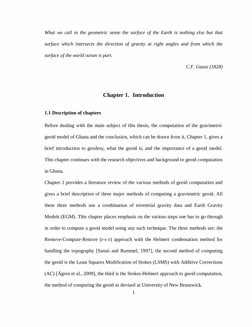
What we call in the geometric sense the surface of the Earth is nothing else but that
surface which intersects the direction of gravity at right angles and from which the
surface of the world ocean is part.
C.F. Gauss (1828)
Chapter 1. Introduction
1.1 Description of chapters
Before dealing with the main subject of this thesis, the computation of the gravimetric
geoid model of Ghana and the conclusion, which can be drawn from it, Chapter 1, gives a
brief introduction to geodesy, what the geoid is, and the importance of a geoid model.
This chapter continues with the research objectives and background to geoid computation
in Ghana.
Chapter 2 provides a literature review of the various methods of geoid computation and
gives a brief description of three major methods of computing a gravimetric geoid. All
these three methods use a combination of terrestrial gravity data and Earth Gravity
Models (EGM). This chapter places emphasis on the various steps one has to go through
in order to compute a geoid model using any such technique. The three methods are: the
Remove-Compute-Restore (r-c-r) approach with the Helmert condensation method for
handling the topography [Sansò and Rummel, 1997], the second method of computing
the geoid is the Least Squares Modification of Stokes (LSMS) with Additive Corrections
(AC) [Ågren et al., 2009], the third is the Stokes-Helmert approach to geoid computation,
the method of computing the geoid as devised at University of New Brunswick.
2
This is followed by Chapter 3, which is dedicated to the UNB Stokes-Helmert’s method
selected for the computation of the gravimetric geoid model of Ghana. This Chapter
starts with a two-space set-up, used for formulating the boundary value problem and
defining gravity quantities, which would be appropriate for downward continuation from
the Earth’s surface to the geoid level. This is followed by the description of the reference
gravity field and the spheroid, and the reformulation of the Stokes’ boundary value
problem for the higher-degree reference spheroid. This includes the various steps
necessary in the UNB’s application of the Stokes-Helmert method in solving the geodetic
boundary value problem of geodesy.
Chapter 4 is dedicated to the description of gravity data used in the computation of the
geoid. This Chapter starts with the background of gravity data acquisition in Ghana. This
includes a brief history of instrument used in the data acquisition, precautionary measures
taken during the data acquisition process, reduction of the raw gravity data, computation
using least squares adjustment and the standard deviation of the junction points. It is
explained that in order to refer the computed gravity values to the Potsdam system, a link
was established between the gravity survey network in Ghana with that of the United
Kingdom. Computations such as Free-air gravity anomalies required for the computation
of the geoid then follows. This computation process also includes the description of
software used in gridding the gravity data, the Earth Gravity Models (EGMs), and SRTM
gridded data at different densities, needed in the computation by the SHGeo software.
Chapter 5 follows with a discussion and assessment of the results of the computed geoid
model. This assessment also includes a recommendation about the need to improve this
computed geoid model, in the near future, by including the airborne gravity data in any
3
new computation of a geoid model for Ghana. It also contains the essential problems
encountered when assessing the accuracy of this geoid model, as there is a lack of
GPS/levelling data that would covers the entire country. This Chapter concludes with
recommendation for further work, which have to done to improve the geoid model.
1.2 Background
Geodesy as defined by Friedrich Robert Helmert (1880) is the science that deals with the
measurement and representation of the earth’s surface. Torge, [2001] extends this
definition to include the determination of the gravity field of the earth in a three
dimensional time varying space. This extension of the definition of geodesy by Torge
follows up on a definition of geodesy introduced by Vaníček and Krakiwsky [1986].
However, geodesy has been around for centuries. Humankind has been concerned about
the earth on which they live and carry out virtually all their activities. During very early
times, most of these human activities were limited to his or her immediate vicinity. The
development of means of transportation enabled human to travel to distant lands, and as a
results, humans became interested in the size and shape whole world [Burkhard, 1985].
According to Homer (B.C. c.900-800) the Earth was a convex dish surrounded by an
infinite ocean which he called Oceanus [Bullen, 1975]. Thales (c.625-c.547 B.C) of
Miletus provides the first document about Homer’s ideas regarding the shape of the earth.
To Thales the earth is a disc-like body floating on an infinite ocean [Vaníček and
Krakiwsky, 1986]. To Anaximander (B.C. 610-547), a contemporary of Thales, the earth
was cylindrical with the axis oriented in an east-west direction [Vaníček and Krakiwsky,
4
1986]. Anaximander was the first to advocate the notion of a celestial sphere, - an idea
that permeated astronomical thinking in his era [Bullen, 1975]. Anaximenes, a pupil of
Anaximander, believed strongly that the earth was rectangular and the earth is floating on
an infinite, circumferential ocean held in space by compressed air [Vaníček and
Krakiwsky, 1986]. Pythagoras (a mathematician) believed that the earth shape is
spherical. According to Burkhard, [1985], Pythagoras reasoned that the gods would
create the most prefect figure, and this perfect figure to him was a sphere. Aristotle
supported this idea of a spherical earth by Pythagoras about a hundred years later. After
accepting the theory of a spherical earth, came the efforts to determine the length of its
circumference. Eratosthenes left an account of a method of estimating the circumference
of the earth. Plato, Archimedes and Posidonius also contributed in determining the
circumference of the earth. It is now accepted that the earth is flattened at the poles and
bulges around the equator. The geometrical figure used in geodesy to nearly approximate
the shape of the earth is an ellipsoid of revolution [Vaníček and Krakiwsky, 1986].
Because of the above definition, geodesy is considered to have two parts: The first part,
which concerns measurement and representation aspect, is often referred to as
geometrical geodesy. Geometrical geodesy deals with the determination of the size and
shape of the earth, intercontinental ties among land masses of the earth, and the
determination of positions, lengths of lines, and azimuths [Ewing and Mitchell, 1970].
The second part called physical geodesy, is the study of the shape of the earth and its
gravity field. In studying the gravity field of the earth, use is made of gravity anomalies
and other data. Physical geodesy is primarily concerned with the use of gravity
measurements and dynamic satellite geodesy to determine the shape of the geoid and
5
deflection of the vertical [Cross, 1985]. The aims of physical geodesy according to
[Bomford,1975] include:
1. Studies of the variations in the intensity and direction of gravity at the earth’s
surface and the determination of the irregularities in the form of the geoid and the
external equipotential surfaces.
2. The variations in the intensity and direction of gravity with time, which
contributes directly to control of geodetic framework through Stokes’s and related
integral.
3. Some consideration of the variation of the density in the crust, which cause the
irregularities found. This study is augmented by other geophysical data.
4. Measurements of horizontal and vertical movements at the Earth’s surface
including tides.
5. The use of artificial satellites to study the variation in the intensity and direction
of gravity at the Earth’s surface and the irregularities in the geoid.
In studying the gravity field of the earth, use is made of gravity potential rather than
gravity, which is a vector quantity. The use of potential of gravity is to enable easier
handling of the potential mathematically, because the difference between the actual
and normal potential, called the disturbing potential is quite small [Vaníček and
Krakiwsky, 1986]. Thus, the gravity potential of the earth can be separated into two
parts: one due to normal potential and the other arising from the mass distribution
within the Earth [Bomford, 1975]. Potentials of topographic masses form the
theoretical basis for reducing gravity measured on the surface of the earth to the
geoid. The gradient of the potentials gives gravity and this gravity is needed for the
6
computation of the geoid. Additionally, the gradient of the gravity gives the
differential equation whose solution is required in free space in order to compute the
geoid.
1.3 The geoid
Even though the study of gravity is useful in determining the shape of the earth but not
the size, the determinations of shape and the size of the earth are not independent objects
of study. Geodesists are interested in gravity because the outcome of geodetic
measurements – sets of coordinates, the length, and azimuth of a line, are carried out on
the Earth’s physical surface in the domain of action of terrestrial gravity. While it is
necessary to make observations and measurement on or near the physical surface of the
earth, it is impossible to perform detail mathematical computation on the Earth’s physical
surface. This is because the surface of the earth is extremely uneven and not definable
mathematically [Cross, 1985]. A possible surface for computation is mean sea level or
the geoid. The geoid is defined as the equipotential surface of the Earth’s attraction and
rotation, which on the average coincides with Mean Sea Level of the Earth in the absence
of external influences such as wind and ocean current [Vaníček and Krakiwsky, 1986].
According to Gauss, the geoid is the mathematical figure of the earth [Burkhard, 1985].
Geodesy places a significant emphasis on the geoid, because of its role as the reference
surface for height systems. Orthometric height is defined a distance between the geoid
and the point of interest measured along the plumb line [Vaníček and Krakiwsky, 1986].
7
Most countries in the world use orthometric height for their national height system. The
geoid is physically meaningful because it is tied to the Earth’s gravity field through the
plumblines, and also represents the level at which seawaters would stabilize if they were
homogenously at rest [Kingdon, 2012]. A level surface is everywhere horizontal i.e.
perpendicular to the direction of the plumb line. Level surfaces are surfaces of constant
potential and the geoid is one of them [Moritz, 1990].
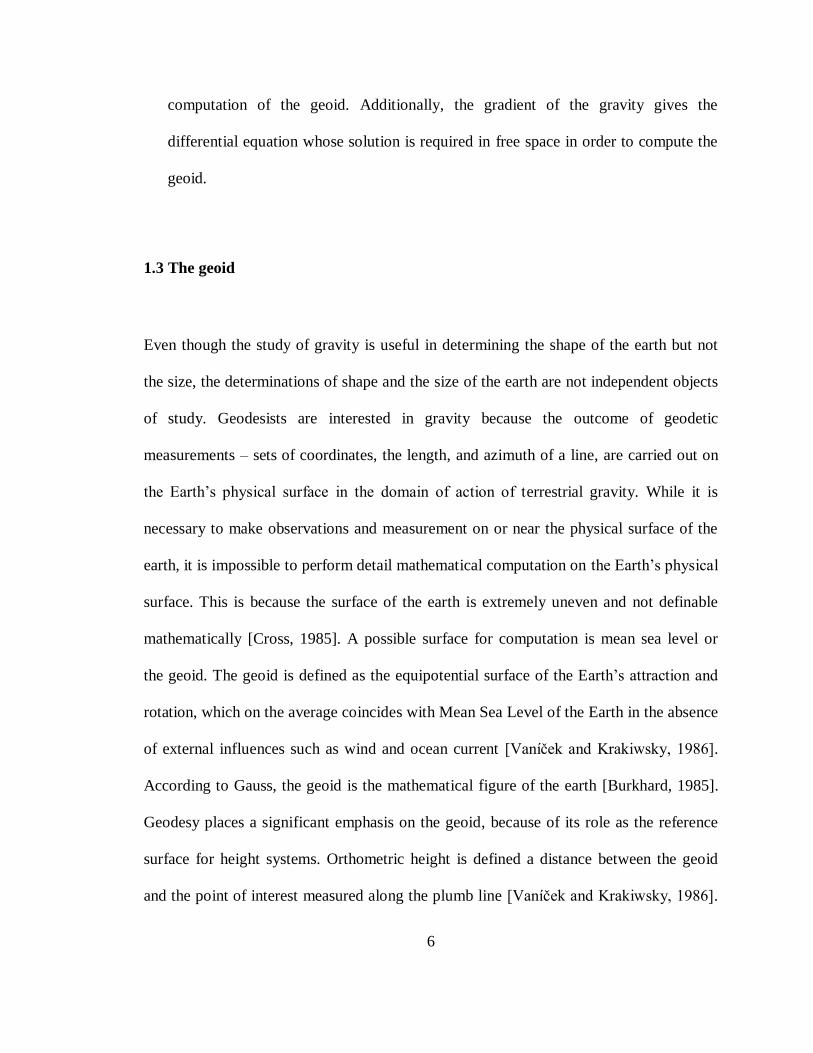
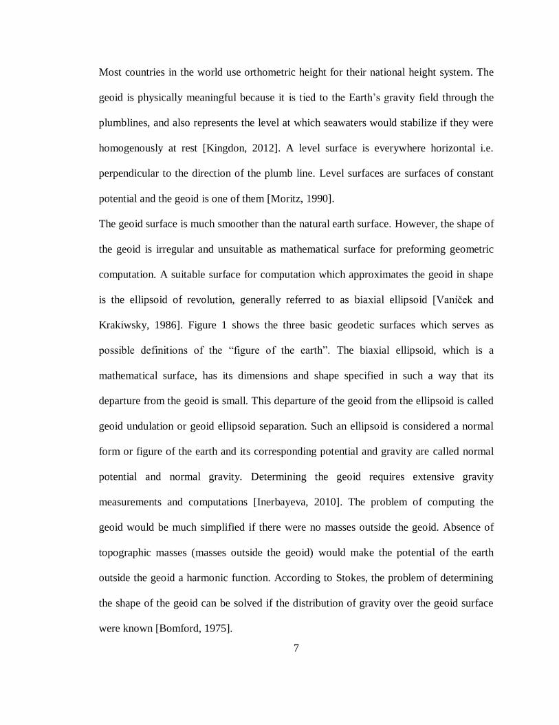
The geoid surface is much smoother than the natural earth surface. However, the shape of
the geoid is irregular and unsuitable as mathematical surface for preforming geometric
computation. A suitable surface for computation which approximates the geoid in shape
is the ellipsoid of revolution, generally referred to as biaxial ellipsoid [Vaníček and
Krakiwsky, 1986]. Figure 1 shows the three basic geodetic surfaces which serves as
possible definitions of the ―figure of the earth‖. The biaxial ellipsoid, which is a
mathematical surface, has its dimensions and shape specified in such a way that its
departure from the geoid is small. This departure of the geoid from the ellipsoid is called
geoid undulation or geoid ellipsoid separation. Such an ellipsoid is considered a normal
form or figure of the earth and its corresponding potential and gravity are called normal
potential and normal gravity. Determining the geoid requires extensive gravity
measurements and computations [Inerbayeva, 2010]. The problem of computing the
geoid would be much simplified if there were no masses outside the geoid. Absence of
topographic masses (masses outside the geoid) would make the potential of the earth
outside the geoid a harmonic function. According to Stokes, the problem of determining
the shape of the geoid can be solved if the distribution of gravity over the geoid surface
were known [Bomford, 1975].
8
Figure 1-1 The surface of the Earth, geoid and ellipsoid Source: [Burkhard, 1985
1.4 Uses of a geoid model
An essential problem of physical geodesy is the determination of the gravity field of the
earth from various types of measurements by solving a boundary value problem. The aim
in solving this boundary value problem is to get a geoid model accurate to one centimeter
level. The wide use of GPS for geodetic heighting is considered to be the main reason for
a centimeter geoid model. Conversion of geodetic heights, (the height system in which
GPS determined heights are given), to orthometric heights requires an accurate geoid
model. The importance of determining a geoid model can be explained as follows:
9
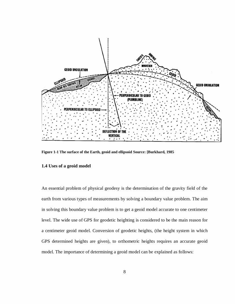
1. The use of GPS has replaced the time consuming traditional methods of surveying
which has transformed the fields of survey and mapping, navigation and
Geographic Information Systems (GIS). Having a geoid model enables effective
use of GPS determined heights in some applications where is possible to use
GNSS for surveying, such as when is possible to receive the signals from the
satellites, and avoids the use of traditional methods of levelling in some cases,
which are expensive as compared to the use of GPS [Abdalla and Fairhead, 2011].
2. Gravity field information is necessary for predicting the positions of satellites in
their orbit. Since the geoid reflects the various variations in the gravity field of the
Earth, a good understanding of the geoid enables a better prediction of the
satellites in the orbits [Inerbayeva, 2010].
3. Knowledge of the geoid is essential for modelling hydrographic surveys and
marine navigation.
4. The geoid serves as the reference surface of orthometric heights.
5. Variations in the gravity field are due to changes in density of matter within the
Earth. This serves as valuable information for locating natural resources such as
ore deposits as well as oil and gas [Inerbayeva, 2010].
1.5 Research objective and contribution
In Ghana almost all survey works, especially horizontal control positioning, are carried
out using GPS. Yet the main method of determining heights for benchmarks for all
10
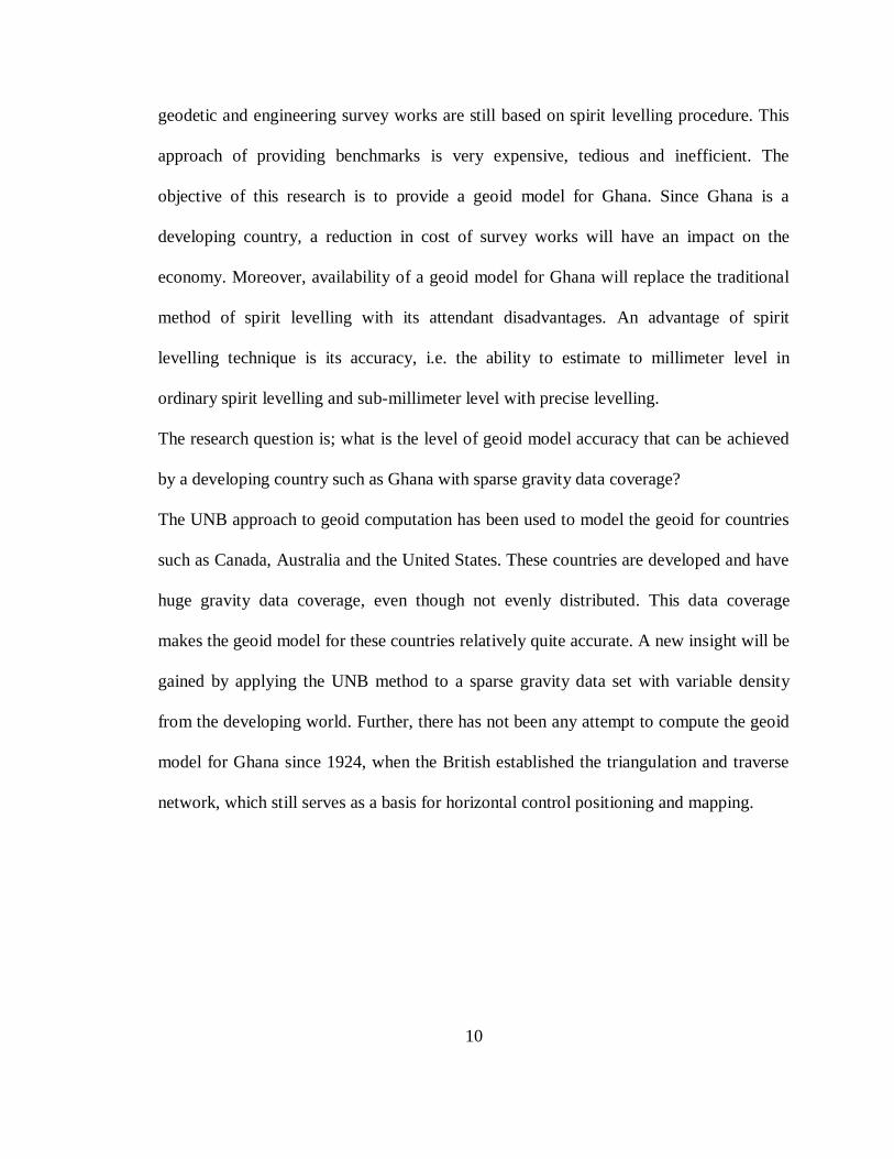
geodetic and engineering survey works are still based on spirit levelling procedure. This
approach of providing benchmarks is very expensive, tedious and inefficient. The
objective of this research is to provide a geoid model for Ghana. Since Ghana is a
developing country, a reduction in cost of survey works will have an impact on the
economy. Moreover, availability of a geoid model for Ghana will replace the traditional
method of spirit levelling with its attendant disadvantages. An advantage of spirit
levelling technique is its accuracy, i.e. the ability to estimate to millimeter level in
ordinary spirit levelling and sub-millimeter level with precise levelling.
The research question is; what is the level of geoid model accuracy that can be achieved
by a developing country such as Ghana with sparse gravity data coverage?
The UNB approach to geoid computation has been used to model the geoid for countries
such as Canada, Australia and the United States. These countries are developed and have
huge gravity data coverage, even though not evenly distributed. This data coverage
makes the geoid model for these countries relatively quite accurate. A new insight will be
gained by applying the UNB method to a sparse gravity data set with variable density
from the developing world. Further, there has not been any attempt to compute the geoid
model for Ghana since 1924, when the British established the triangulation and traverse
network, which still serves as a basis for horizontal control positioning and mapping.
11
According to our opinion we have to determine numerically in the future the derivations
of the plumbline as long as they have visible origin, namely by a topographic surface of
the continental relief, by a geological determination of the mass density of its constituents
and by a systematic survey of the oceans according to well-established method….We
shall call the previously defined mathematical surface of the earth, of which the ocean
surface is a part, geoidal surface of the Earth or the geoid.
J.B. Listing (1873)
Chapter 2. Literature review
2.1 Introduction
Ideas about the geoid as the mathematical surface of the earth as distinguished from the
ellipsoid had been developed and expounded by renowned mathematicians of the
eighteenth century such as Gauss (born 1777) and Bessel(born 1784) [Moritz, 1990]. The
question then is how is the separation between the geoid and the referenced ellipsoid
determined? One approach towards a solution is astro-geodetic method. However, such a
solution would only be possible on the continents.
A theory by G. G. Stokes [1849] made it possible to compute the geoid-ellipsoid
separation throughout the world. His determination of the geoid is based on gravity
observations [Vaníček and Christou, 1993].Since that time, the mathematical methods,
observation techniques and modelling methods have made a great progress. The
12
availability of satellites trajectory data since the 1960s has led to an increased knowledge
of the long wavelength shape of the geoid and also made the computation of the geoid
possible since Stokes approach to geoid determination will require gravity data
throughout the Earth [Amalvict and Boavida, 1993].
This chapter starts with a discussion on the need for a centimeter geoid and the
difficulties in achieving such accuracy in computing the geoid computation [Sansò and
Rummel, 1997]. Molodensky maintained that an accurate geoid computation has to take
into account topographical density variations which would always be unknown. To what
level of accuracy then could the geoid be modeled? Research at UNB has shown that
Helmert’s second condensation method, when used in combination with the theory by
Stokes, works reasonably well for reducing the effect of limited knowledge of the
topographic density on the accuracy of geoid determination [Vaníček et al., 2013]. This
chapter concludes with a review of other techniques of geoid computations such as
remove-compute-restore approach and the Least Squares Modification methods together
with a brief comment on the limitations of the remove-compute –restore technique as
well as questions regarding the validity of the theory behind the Least Squares
Modification technique.
2.2 The goal for centimeter geoid
Currently, one of the biggest tasks facing the geodetic community is the determination of
a centimeter geoid model. A deficiency in the accuracy of geoid models limits the use of
Global Navigation Satellite System (GNSS) technology, i.e., the technique to do leveling
13
using GNSS technology and the gravimetric geoid model [Sjöberg, 2013]. Advances in
GNSS technology made it possible to determine geodetic height with an accuracy of a
few centimeters depending on the observation and processing techniques. Improvement
in technology may lead to increased accuracy in GNSS positioning in the future. This
improvement in accuracy will also require more accurate geoid models. The solution to
this height problem will enable the geodetic community to benefit fully from GNSS
technology.
However, this quest for the centimeter geoid determination is not easy, particularly in
mountainous regions. Knowledge of the mass density distribution within the Earth’s
topography is required in order to compute such an accurate geoid. Unfortunately, the
density distribution within the Earth is not known to sufficient accuracy [Kingdon, 2012].
As the detail density distribution of the topography is unknown, Molodensky developed
his famous technique by introducing the quasi-geoid.
However, according to Vaníček et al.[2012] determining the quasi-geoid using the
Molodensky method has a fatal problem with the geometry of the Earth’s surface.
Integrating gravity over the surface of the Earth, which is much rougher then the geoid is
not possible in certain areas, and in other areas will result in unpredictable errors. They
argue that vertical rock surfaces represent locations of discontinuity, and there are other
areas where the surface of the Earth cannot be described as a mathematical function of
horizontal positions. In these locations, the Molodensky technique fails. Hence, in their
opinion, the geoid which is a fairly smooth and convex surface, without any kinks, edges
or other irregularities, is a better surface for integration [Vaníček et al., 2012]. There have
been several attempts to address this density distribution within the topography issue.
14
Martinec [1993] made his first attempt to model the topo-density effects of lateral
(horizontal) anomalies. Martinec’s approach modeled the topography as discrete mass
columns. Huang et al.[2001], carried out a practical application of Martinec’s ideas in
western Canada. Other advanced technique of topographical density modelling includes
rectangular parallelepiped prism by Nagy et al.[2000], prisms with inclined surfaces (e.g
[Smith, 2000]) and bilinear surfaces (e.g [Tsoulis et al., 2003]). All these techniques
enable computation of any three-dimensional density distribution of topographic masses
to the desired accuracy using close formula [Nagy et al., 2000]. Additionally, densities
could be assigned to each prism independent of any neighboring densities. Since no
close-form solution for prism whose tops are in shape of a curve has been found, all the
above mentioned techniques use plane surfaces in modelling the density effects, which is
an approximation for the true topography [Smith, 2000]. Research at UNB towards the
use of laterally-varying Digital Density Model (DDM) of the topography for geoid
modelling, created by digitizing geological maps and assigning appropriate rock densities
were carried out by Fraser et al.[1998], Tenzer et al.[2005], Santos et al.[2006]. Their
methods are comparable to that due to Martinec [1993]. They reported that the effect of
lateral density variation on the geoid computation is at most a few decimeters with a
standard deviation of less than 2 centimeters [Kingdon, 2012]. Additionally, Martinec et
al.[1995] investigated the influence of the radial changes of densities of topographic
masses between the geoid and the Earth’s surface (vertical density variation). They
reported a variation of less than 5 cm even under very extreme conditions, and under
realistic conditions, are not likely to exceed 2-3 cm [Kingdon, 2012]. Again, research by
Vaníček et al.[2013] using a synthetic gravity field shows that the geoid could be
15
modeled to a standard deviation of about 25 mm and a maximum range of about 200 mm.
It is important to mention that these researchers did not use any corrective measures, such
as surface fitting or biases and tilts, so the resulting errors reflect only the errors in
modelling the geoid.
Thus, the quest for centimeter geoid is possible if topo-density information is
incorporated in the geoid computation. As shown by the researchers at UNB, the
topographic density issue can be resolve to a few centimeters if the density within the
crust is reasonably well known [Kingdon, 2012].
2.3 Techniques for geoid computation
Methods of computing the geoid depends on the data used for the computation process.
This includes terrestrial gravity data, airborne and marine gravity data, deflections of the
vertical, GNSS/levelling data and satellite data. The data sources can be combined in one
form or another to determine the geoid. Marchenko et al.[2002] combined airborne
gravity data with gravity data obtained by different techniques to compute the geoid.
Sjöberg and Eshagh, [2009], also investigated computation of a geoid model from
airborne gravity data. Their technique combined airborne gravity data with satellite
positioning data points. Hirt et al.[2009] validated a geoid model for mountainous region
of the German Alps using astrogeodetic method of geoid computation. They determined
vertical deflection at 100 stations (with a spacing of about 230m) arranged in a profile of
23 km length. Repeated observation at 38 stations in different nights revealed an
observational accuracy of about 08.0 . Comparison of the computed astrogeodetic profile
16
with GPS/levelling data yielded differences of 10 mm. Abd-Elmotaal and Kühtreiber
[2014] used Airy isostatic hypothesis to topographically-isostatically reduce the
deflection of the vertical observations. The reduced deflections were used to interpolate
deflection of the vertical to form a dense grid. The gridded reduced deflections were used
to compute astrogeodetic geoid. They report a good fit with GPS/levelling data.
Terrestrial gravity data set have been used to compute the geoid for several countries
around the world. Remove-compute-restore and least squares modification methods are
two main approaches used when computing the geoid using terrestrial gravity data and a
review of these methods are shown in section 2.4.
2.4 Remove-compute-restore using Stokes-Helmert method of geoid computation
The National Survey and Cadastre of Denmark (KMS) and the Geophysics Department
of the Neils Bohr Institute of University of Copenhagen developed the pure remove-
compute restore (r-c-r) method of geoid computation [Forsberg, 1985]. There are several
approaches to geoid model computation using the r-c-r technique. Each of these
techniques handles the topography in a different way prior to gravity anomaly data being
used as input into the Stokes formula. The basic steps of geoid computation using
remove-compute-restore and Helmert condensation technique for handling the
topography are as follows:
1. Remove the effect of topography from the gravity data on the surface of the earth
Calculate free-air gravity anomalies from the gravity observation data.
17
Convert the free-air gravity anomalies to Bouguer gravity anomalies using
planar approximation. Planar Bouguer anomaly is smoother than free-air
anomaly and thus easier to grid.
Grid the planar Bouguer gravity anomaly
Convert the gridded planar Bouguer anomaly back to free-air gravity
anomaly
Apply Helmert second condensation method to remove the effect of the
topography above geoid to satisfy the boundary conditions of Stokes
integration
2. Compute the downward continuation of the gridded gravity anomalies
3. Remove the long-wavelength part of the gravity signal from the terrain reduced
gravity data
The long-wavelength part of gravity signal predicted from the geopotential model
up to a chosen spherical harmonic degree and order is removed from the terrain
reduced gravity anomalies. The result is referred to as residual gravity anomaly.
4. Compute the residual co-geoid by applying Stokes integral. The residual co-geoid
undulations are calculated from the residual gravity anomalies using a modified
Stokes function.
18
5. Restore the long-wavelength part of the gravity signal subtracted earlier using the
same EGM to the same degree and order by computing the reference spheroid.
6. Compute the primary indirect topographic effect on the geoid.
7. Obtain the gravimetric geoid by adding the residual co-geoid, the reference
spheroid and the primary indirect topographic effect on the geoid.
The scheme of remove-compute-restore using Helmert condensation described above
suffers from truncation errors because the process neglects the far-zone contribution in
the computation of the residual co-geoid. A more rigorous approach, which accounts for
the far-zone contribution, is the Stokes-Helmert method of geoid computation developed
at UNB.
2.5 Least Squares Modification Method (LSMS) also called KTH method
The Royal Institute of Technology (also known as KTH), in Sweden, developed the KTH
method of geoid computation. This KTH method is also called Least Squares
Modification with additive corrections. This technique of geoid computation is based on
gravity anomaly data. However, the technique does not require gravity reduction but
rather includes additive corrections for the topographic effect, downward continuation,
atmospheric and ellipsoidal corrections for the shape of the earth [Yildiz et al., 2012]. A
review of the computation steps for geoid modelling using the KTH method according to
Ågren et al. [2009] is as follows
19
1. Compute gravity anomalies from the gravity observation data
2. Use a gridding algorithm to grid the gravity anomalies data
3. Compute an approximate geoid-ellipsoid separation using the terrestrial gravity
anomalies and the Earth Gravity Model gravity anomalies up to degree and order
M. In computing the approximate geoid separation, a modified Stokes kernel is
used.
4. Compute the combined correction due to the topographic effect using DEMs.
5. Compute the downward continuation effect
6. Compute the atmospheric effect
7. Compute the ellipsoidal correction to the modified Stokes formula
8. Compute the geoid by adding all the corrections to the approximate geoid
computed in step 3
As indicated earlier, the above-mentioned steps of computing the geoid, the Least
Squares Method applies corrections to the approximate geoid computed from surface
gravity anomalies directly, without applying any of the traditional gravity reductions
prior to Stokes integration, such as downward continuation of the reduced gravity
anomalies. Furthermore, the method does not apply indirect effects of the topography and
20
the atmosphere [Inerbayeva, 2010]. According to Sjöberg, [2003], the aim of this Least
Squares Modification approach to geoid computation is to modify (find a new approach)
to the traditional procedure used in geoid computation in view of a centimeter geoid
model. A big question is whether this procedure has a sound theoretical foundation. As
pointed out in the reference made in section 4.12, downward continuation of gravity
anomalies is only possible if there are no masses within the range of the continuation
process.
Over the past two decades, researchers at University of New Brunswick have used the
Stokes-Helmert approach to geoid computation. Their approach uses a two-space set-up;
real space, used for defining gravimetric quantities, appropriate for downward
continuation from the Earth’s surface to the geoid level, i.e., solid gravity anomalies, and
Helmert’s space (see below) for formulating and solving the Stokes boundary value
problem [Ellmann and Vaníček, 2007]. In addition, the topographic effects are
formulated in their spherical form. Their solution to the Stokes boundary value problem
employs a modified (but differently from Sjoberg’s modification) Stokes’s formula in
conjunction with the low-degree contribution from an Earth Gravity Model (EGM). They
reported that their approach through testing and the technique in the mountainous
regions of Canada and on the Australian synthetic gravity field, is suitable for
determining geoid model with a standard deviation of centimeter accuracy geoid
depending on the availability of terrestrial gravity data coverage and quality of the
gravity data [Vaníček et al., 2013]. The next chapter gives a detailed theoretical basis for
the UNB Stokes-Helmert approach to geoid computation.
For a long time mathematicians felt that ill-posed problems cannot describe real
phenomena and objects.
A.N. Tikhonov and V.Ya. Arsenin, 1977
Chapter 3. Theoretical background of Stokes-Helmert’s approach to
geoid determination
3.1 Introduction
The theoretical foundation which forms the basis for the computation of the geoid was
derived by Stokes in 1849 [Vaníček and Christou, 1993]. According to this theory, the
geoid can be obtained from gravity observation on the geoid and there should be no mass
outside the geoid [Tenzer et al., 2003]. This condition is difficult to attain since gravity
measurements are carried out on the surface of the Earth. To satisfy this boundary
condition specified by the theorem, gravity anomalies need to be downward continued
from the surface of the Earth to the geoid. Harmonic quantities are needed for the
downward continuation and thus a number of different corrections related to the existence
of topography and the atmosphere needed to be accounted for carefully [Ellmann and
Vaníček, 2007].
This reduction process requires knowledge of topographical mass density, which can be
assumed from geological maps, and they assure quite a high accuracy of the geoid
computation [Huang et al., 2001]. Helmert [1884] in his first attempt to satisfy this
condition suggested that the Earth’s topographical masses and atmosphere can be
replaced by a condensation layer of an infinitesimal thickness located inside the geoid.
This condense mass layer has areal density which equals the product of the mean density
of the topographical column and the height (orthometric) of topographical column above
the point [Vaníček and Martinec, 1994]. In his second condensation model, Helmert
placed the condensation layer on the geoid [Heck, 1993]. Martinec and Vaníček, [1994a]
used Newtonian attraction to formulate the effect of topography on the gravitational
potential for laterally varying topographical density distribution for the spherical
approximation of the geoid.
Vaníček et al.[1987] used an idea introduced by Molodensky, which seeks to modify the
Stokes function, by introducing higher degree gravity field as a reference field. The
theory of the reference gravity field, the reference spheroid and the reformulation of the
Stokes’s boundary value problem for the higher-degree reference spheroid have been
described by Vaníček and Sjöberg, [1991], and Vaníček and Featherstone, [1998]. The
boundary-values, Helmert’s gravity anomalies on the geoid, are computed by the use of
the Poisson integral equation for the downward continuation.
The principle of the Stokes-Helmert’s scheme for geoid computation according to Tenzer
et al., [2003] can be summarized as follows:
1. Formulation of the boundary-value problem in real space.
2. Transformation of the boundary-value problem from the real into a harmonic
space, i.e., transformation of gravity anomalies from the real to Helmert space
(according to the second Helmert’s condensation technique where the
topographical and atmospheric masses are condensed directly onto the geoid),
which consist of adding the Direct Topographic Effect, Direct Atmospheric Effect
and other smaller effects to the free-air anomalies on the Earth surface. Helmert’s
anomalies are not very different in character from the real free-air anomalies.
3. Solution of Dirichlet’s boundary-value problem, i.e., the downward continuation
of Helmert’s gravity anomalies from the surface of the Earth to the geoid, by
applying the Poisson integral equation. This is the most difficult of the whole
process.
4. Reformulation of the geodetic boundary-value problem by decomposition of
Helmert’s gravity field into low frequency and high frequency parts. It should be
noted that the residual anomalies are somewhat smaller than the original
anomalies.
5. Solution of the Stokes boundary-value problem for the residual (high-frequency)
Helmert gravity field (by using the modified spheroidal Stokes kernel) and
whereby the residual Helmert geoid, called Helmert residual co-geoid is thus
referred to the reference spheroid (obtained from satellite geopotential model) of a
degree L. The complete Helmert co-geoid is obtained by adding together the
Helmert reference spheroid and the Helmert residual co-geoid.
6. Transformation of the complete Helmert co-geoid from Helmert space into the
real space. This is done by adding the Primary Indirect Topographic Effect (PITE)
to complete Helmert’s co-geoid.
3.2 Formulation of geodetic boundary-value problem in real space
This problem is formulated as determining the geoid by transforming the Stokes
boundary value problem into Helmert space where the Stokes boundary value problem
represents the standard free boundary value problem of geodesy. The formulation closely
follows that of Vaníček and Martinec, [1994].There are an infinite number of
equipotential surfaces of the of the earth’s gravity field on which of course the potential
is constant. Among them, there is only one surface which approximates the mean sea
level most closely and it is given a special significance. This surface is denoted by
.constWW o (3.1)
and is called the geoid.
Similarly, there are an infinite number of equipotential surfaces of the normal gravity
field. Among these, there is only one such surface which coincides with the reference
ellipsoid and is denoted by
gWU (3.2)
This normal gravity field is selected such that it satisfies the Poisson equation outside the
generating ellipsoid:
22 2 U (3.3)
where is the gradient operator. The normal gravity denoted by is the gradient of U.
The difference between the Earth’s gravity potential, ),,( rW and normal gravity
potentials, ),,( rU is called the disturbing potential denoted by ),,( rT and reckoned
anywhere is written as
),(),(),( rUrWrT (3.4)
where r is the geocentric distance (radius), is the geocentric angle denoting the pair
),( — the spherical co-latitude and longitude. In this sequel, the arguments ( ,r ) is
the position in three dimensions. In solving the geoid and related corrections, the
mathematical operations often needs to be taken over a total solid angle
]2,0,2,2[0 .
The disturbing potential satisfies the Laplace equation outside the earth and its
atmosphere. In the absence of topographic masses and the earth’s atmosphere, the
disturbing potential will be harmonic above the geoid so that
0),(2 rT (3.5)
where denotes the gradient operator.
If the values of the disturbing potentials are known of the geoid, the geoid ellipsoid
separation can be computed using Bruns’s formula
)(
),()(
0
grTN (3.6)
where )(0 is the normal gravity on the reference ellipsoid. Since the disturbing
potential cannot be measured directly, then a boundary value problem of the third kind
has to be formulated and solved. In geoid determination some type of gravity anomalies,
referred to the geoid level serve as the boundary values of this problem [Martinec et al.,
1993]. To find the relation between the disturbing potential and the gravity anomalies, the
radial derivative of the disturbing potential is introduced:
r
rU
r
rW
r
rT
),(),(),( (3.7)
Equation 3.7 evaluated at the surface of the Earth can be approximated according to
[Vaníček and Novák, 1999] by
),(),(),(),(),(),(
tgttgtt
rr
rrgrrrgr
rT
t
(3.8)
where the difference between the actual gravity, ),,( trg and normal gravity, ),,( tr is
the gravity disturbance, ),,( trg and ),( tg r is the ellipsoidal correction (due to the
replacing of the derivative with respect to ellipsoidal normal n by a more convenient
derivative with respect to r) to the gravity disturbance. The geocentric radius is obtained
by adding the orthometric height, ),(oH to the )(gr ,i.e., )()()( o
gt Hrr . The
approximation is due to )(oH being measured along the plumb-line between the geoid
and the surface of the Earth, which is somewhat curved.
3.3 Gravity anomaly
In the pre-GNSS era, geodetic height was not available and gravity anomalies rather than
gravity disturbances had to be used. The world data bases are full of gravity anomalies
and there are few gravity disturbances. The reason is that normal gravity cannot be
evaluated on the surface of the earth, as this requires the knowledge of the geodetic
height h of the point. Hence, the gravity anomalies have to be transformed into gravity
disturbance [Vaníček and Novák, 1999].
In general, gravity is measured on the surface of the earth. Before these measurements
can be used for geodetic or geophysical purposes, they must be converted into gravity
anomalies. Geophysics use gravity anomalies to deduce variations in the mass within the
earth. This helps in interpretation of the underlining subsurface structure. For geodesist,
gravity anomalies are used to define the figure of the Earth, the geoid [Hackney and
Featherstone, 2003]. Furthermore, Gravity anomalies are differentiated according to the
way in which the observed or normalous gravity was deduced. Surface gravity anomaly
does not require the knowledge of the vertical gradient of the actual gravity within the
earth.
The exact value of the normal gravity on the telluroid needed for surface gravity anomaly
is obtained from normal height NH . Normal height is computed by upward continuation
of normal gravity from the geocentric reference ellipsoid [Vaníček and Krakiwsky,
1986]. Gravity anomalies are calculated from gravity measurements on the surface of the
earth as
),(),(),( tTtttt rrgrg (3.9)
where ),( ttrg is the observed gravity on the surface of the earth and ),( tTr is the
normal gravity evaluated on the telluroid. Normal gravity is a theoretical value
representing the acceleration of gravity that is generated by the reference ellipsoid
according to Somigliana-Pizzetti theory. Normal gravity on the ellipsoid is evaluated by
the use of Somigliana formula due to Somigliana. The formula from Vaníček and
Krakiwsky [1986] reads
2222
22
sincos
sincos
ba
ba ba
(3.10)
where a, b are the major and minor semis-axes of the ellipsoid, and ba , are normal
gravity at the equator and the pole of the ellipsoid respectively.
Since the Somigliana’s formula determines the normal gravity on the reference ellipsoid,
a height correction is needed to account for a change in theoretical gravity due to the
location of the telluroid above or below the ellipsoid. Historically, this height correction
has been incorrectly associated with the orthometric height H, not the geodetic height h
[Li and Götze, 2001]. As a second approximation using a Taylor series expansion for the
theoretical gravity above the ellipsoid with a positive direction downward along the
geodetic normal to the reference ellipsoid according to [Heiskanen and Moritz, 1967] is
given by
2
2
2 3)sin21(
21 h
ahfmf
ah (3.11)
The difference h is the correction for height above the reference ellipsoid.
According to [Moritz, 1980] this height correction is given by
2
2
2 3sin3
2
51
2h
ahfmf
a
eh
Substituting the values for the GRS80 ellipsoid into Eq. (3.12) gives
(3.12)
282 102125.7)sin0004398.03087691.0( hhh
(3.14)
The transformation of gravity disturbance to gravity anomaly is achieved by adding a
term to the gravity disturbance that accounts for the change in normal gravity due to the
difference between the geodetic height h and the orthometric height oH [Vaníček and
Novák, 1999]. The gravity anomaly is thus related to the gravity disturbance, ),( trg
by the following formula:
)]()([),(),(),( 0 N
ttt Hrrrgrg (3.15)
where NH is normal height and )(0 r is the geocentric radius (a function of latitude) of
the reference ellipsoid.
Using Molodensky’s approach, the difference of the normal gravity ),( tr on the
Earth’s surface: ),()()()()( hrHrr o
o
gt and normal gravity ))(( NH
on the telluroid in Eq. (3.15) can be evaluated as:
)(),(
)())(())(())(()(
OHRr
t
N
tn
rrgradHr (3.16)
where n is the derivative of normal gravity taken with respect to the normal n to the
reference ellipsoid and )( is the Molodenskij height anomaly. Using Bruns’s spherical
formula, the expression on the right-hand side of Eq. (3.16) according to [Vaníček and
Novák, 1999] can be rewritten as
))((
))((),()(
),(
)()(
N
t
HRrHRr H
rT
n
r
n
r
OO
(3.17)
Substituting Eq. (3.17) into Eq. (3.16) leads to
))((
))((),(),(),(
)(
N
t
HRr
ttH
rT
n
rrgrg
O
(3.18)
Applying spherical approximation
),(),()(
2),(
),(
))((
1
)(
tnt
tHRr
NrrT
rrT
n
r
H O
(3.19)
where ),,( tn r the ellipsoidal correction for the spherical approximation allows to
replace the ―ellipsoidal‖ term by a more simple term: ),())(2( rTr . Substituting Eq.
(3.8) and Eq. (3.19) into Eq. (3.18), the fundamental formula of physical geodesy takes
the following form [Ellmann and Vaníček, 2007]
),(),()(
2),(
),(),(
)(
tnt
t
tg
rr
tt rrT
rr
r
rTrg
t
(3.20)
The above equation formulated in real space can be applied in Helmert space for the
purpose of the computation of Helmet’s (and any other) gravity anomaly: ),( t
h rg
3.4 Transformation of gravity anomalies from the real space to Helmert space
On the continents the geoid is mostly located inside the topographical masses. To
compute the geoid by Stokes’ formula requires reduction of the disturbing potential, or
the gravity anomalies to the geoid. This reduction process is called downward
continuation [Sun and Vaníček, 1996]. An important requirement for the existence of the
downward continuation is that the function has be harmonic. The presence of topographic
masses and the atmosphere violate this harmonicity condition. To establish the
harmonicity of the disturbing potential everywhere above the geoid implies that the
atmosphere and the topographic masses have to be eliminated [Ellmann and Vaníček,
2007].
One way of eliminating topography and atmosphere is by estimating the effect of the
topographic masses and the atmospheric effect by means of the Helmert’s second
condensation technique, which condenses the topographical masses onto the geoid. This
technique causes relatively small indirect topographic effect–see later. For this reason,
UNB favors this approach in computation of the geoid [Ellmann and Vaníček, 2007].
The gravity field of the Helmert Earth is different from the real Earth and is given by
),(),(),(),( rVrVrWrW ath (3.21)
where the superscript h denotes the quantities referring to Helmert’s Earth or given in
Helmert’s space, ),( rV t is the residual topographical potential, i.e., the difference
between the potential of the topographical masses and the potential of the condensation
layer as shown below:
),(),(),( rVrVrV ctt (3.22)
Similarly, the residual atmospheric potential ),( rV a is the difference between the
potential of the atmospheric masses and the potential of the atmospheric condensation
layer on the geoid as shown below
),(),(),( rVrVrV caaa (3.23)
Using the analogy with the real Earth, Helmert disturbing potential is defined as
),(),(),(),(),(),( rVrVrTrUrWrT athh
(3.24)
Helmert disturbing potential is harmonic outside the geoid, i.e.,
02 hT (3.25)
Helmert gravity ),( t
h rg is the negative radial derivative of the Helmert gravity
potential, which is parallel to the definition of gravity in the real space [Ellmann and
Vaníček, 2007]. Helmert gravity on the surface of the earth is obtained from observed
gravity on the surface of the earth by adding to the observed gravity ),( trg the direct
topographical effect ),( t
t rA and direct atmospheric effect :),( t
a rA
),(),(),(),(
),(
t
a
t
t
tt
h
t
h rArArgr
rWrg (3.26)
Application of the relation rWg utilized in Eq. (3.26) is only an approximation
since the radial derivative is taken over the complete potential rather than over the
disturbing quantity. This is the reason for using the symbol in Eq. (3.26). The
importance of this relation is that it makes the link between actual gravity (and
corresponding gravity anomaly) and Helmert’s gravity anomaly more transparent.
Further, the derivative in Eq. (3.26) should be taken along the plumbline instead of r. As
a result, there is the need to introduce an ellipsoidal correction due to this approximation
[Ellmann and Vaníček, 2007].
Helmert’s gravity disturbance ),( t
h rg is defined as the negative gradient of the
Helmert disturbing potential and can be described as a sum of the negative radial
derivative of the Helmert disturbing gravity potential ),( t
H rT and the ellipsoidal
correction ),( tg r to the gravity disturbance:
),(),(),(),(),(),(),(
),(
t
a
t
t
tgtttgt
h
t
h rArArrrgrr
rTrg
(3.28)
The relation between the gravity disturbance ),( t
h rg and the gravity anomaly
),( t
h rg in Helmert’s space can be obtained from the fundamental gravimetric
equation of physical geodesy Eq. (3.20) as [Tenzer et al., 2003]
]))(()([
)(),(),(
),(),(
0)()(
hN
t
h
rr
tg
rr
t
h
t
h
Hr
rT
r
rr
r
rTrg
tt
(3.29)
),(),()(
2),(
),(
)(
tnt
h
t
tg
rr
t
h
rrTr
rr
rT
t
(3.30)
Helmert gravity anomalies can be expressed via free-air anomalies ),( rg as [Vaníček
and Novák, 1999]
),(),()(
2),(),(),(
t
a
t
t
t
t
t
tt
h rArVr
rArgrg
),(),(),()(
2
tntgt
a
t
rrrVr
(3.31)
The second and third terms on the right-hand side of Eq. (3.31) are direct and secondary
indirect topographic effects on the gravitational attraction. The fourth and five terms of
Eq. (3.31) are the direct and secondary indirect atmospheric effects on the gravitational
attraction. The non-topographical corrections to the Helmert gravity anomaly are then as
follows: direct atmospheric effect, secondary indirect atmospheric effect, ellipsoidal
correction for the gravity disturbance, and ellipsoidal correction for the spherical
approximation.
Importantly, the product of corresponding Helmert anomaly and geocentric radius,
,rg h is a harmonic function above the geoid and, therefore, such a field can be
continued downwards to the geoid level [Vaníček and Novák, 1999]. Normal heights are
used for estimating the normal gravity in Eq. (3.31) and Eq. (3.15). If orthometric heights
are used rather than normal heights, then a geoid-quasigeoid correction has to be applied
to Eq. (3.31) [Ellmann and Vaníček, 2007].
3.5 Effect of topographical masses on gravitational attraction
Evaluation of Helmert’s gravity anomaly on the surface of the earth according to Eq.
(3.31) will require a computation of the direct effect of attraction of the topography. The
topographical effect on gravitational attraction reckoned on the surface of the earth is
represented by direct and secondary indirect topographical effect, DTE and SITE
respectively [Tenzer et al., 2003]. The effects of topographical masses are formulated in
spherical form, instead of planar approximation. Based on a conclusion by Vaníček et al.,
[2001] the spherical model should be used whenever higher accuracy is required. The
spherical model is closer to reality as the planar model does not allow the formulation of
any physically meaningful condensation models [Ellmann and Vaníček, 2007].
The gravitational attraction of the real topography is evaluated using the Newton integral
over the volume of topography. Additionally, the Newton integral can be split into the
Bouguer shell attraction and spherical roughness term for the computation. This splitting
has been introduced to eliminate the singularity of Newton’s integral which occurs at the
at the computation points. According to Martinec, [1993] the potential of topographic
masses, the condensation of which obeys the law of conservation of masses, can be
estimated as
),( t
t rV
200
02 )(
3
1)(1)(
)(4
R
H
R
HH
r
RG
t
o
O
HR
HRrto drdrrrlG
)(
)(
210
0]),,(),([
O
HR
Rrt drdrrrlG
)(21
0
]),,(),([)( (3.32)
where G is the gravitational constant, ]),,(),([ rrl t and ),( are the spatial
distance and geocentric angle between the computational and integration points, d is
the area of the integration element. The first term on the right-hand side of Eq. (3.32) is
the gravitational potential of the spherical Bouguer shell (of mean density o and the
thickness equal to the orthometric height )(0 H of the computation point). The second
term stands for the gravitational potential of the spherical topographical roughness term
and the third term represents the effect of the anomalous topographical density )(
distribution on the gravitational potential.
Similarly Martinec [1993] states that the potential of the condensation masses can be
written as
),( t
ct rV
200
02 )(
3
1)(1)(
)(4
R
H
R
HH
r
RG
t
o
O
dRrlrr
G ttt
o ]),,(,[3
)()( 133
O
dRrlRr
G tt ]),,(,[
3
)()( 1
33
(3.33)
where the first term on the right-hand side of Eq. (3.33) is the gravitational potential of
the condensed spherical material of single layer (spherical Bouguer shell), the second
term stands for the gravitational potential of the spherical roughness term of the
condensed topographical masses, and the third term represents the effect of the
anomalous condensed topographical density distribution on the gravitational potential.
The secondary indirect topographic effect on gravitational attraction (third term on the
right-hand side of Eq. (3.31)), which refers to the earth’s surface is computed by
subtracting Eq. (3.33) from Eq. (3.32), i.e.
)],(),([)(
2),(
)(
2
t
ct
t
t
t
t
t
t
rVrVr
rVr
(3.34)
3.6 Direct Topographic Effect (DTE)
The direct topographic effect is obtained by taking the difference of the radial derivatives
of Eq. (3.32) and Eq. (3.33). The attraction of the topographical masses according to
[Martinec, 1993] reads
)(
),(
trr
t
t
r
rV
200
0
2
2 )(
3
1)(1)(
)(4
R
H
R
HH
r
RG
t
o
O
t
HR
HRrrr
to drdr
r
rrlG
)(
)(
2
)(
10
0
]),,(),([
O
t
HR
Rrrr
t drdrr
rrlG
)(2
)(
10 ]),,(),([)(
(3.35)
where the first term on the right-hand side is the negative gravitational attraction of the
spherical Bouguer shell. The second term is the gravitational attraction of the spherical
roughness term, i.e., the spherical terrain correction and the third term represents the
effects of the anomalous topographical density )( on the gravitational attraction.
The attraction of the condensed masses can be expressed as
trr
t
ct
r
rV ),(
200
0
2
2 )(
3
1)(1)(
)(4
R
H
R
HH
r
RG
t
o
O
t
dr
RrlrrG
rr
ttto
)(
133 ]),,(,[
3
)()(
O
t
dr
RrlRrG
rr
tt
)(
133 ]),,(,[
3
)()(
(3.36)
where the first term on the right-hand side is the gravitational attraction of the condensed
spherical Bouguer shell, the second term is the gravitational attraction of the spherical
roughness term of the condensed topographical masses, and the third term represents the
effect of the anomalous condensed topographical density distribution on the gravitational
attraction.
It should be noted that the first terms of Eq. (3.35) and Eq. (3.36) are equal. Therefore,
the Bouguer shell contributions cancel each other out when Eq. (3.35) is subtracted from
Eq. (3.36). The final expression for the direct topographic effect in Helmert’s space then
becomes
r
rVrVrA t
ct
t
t
t
t )},(),({),(
)(
)(
2
)(
1 ),,(,[HR
HRrr
o drdrr
rrlG
t
O
t
dr
RrlrrG
rr
ttto
)(
133 ]),,(,[
3
)()(
O
t
HR
Rrr
t drdrr
rrlG
)(2
)(
1 ]),,(),([)(
O
t
dr
RrlRrG
rr
tt
)(
133 ]),,(,[
3
)()(
(3.37)
The first term on the right-hand side of Eq. (3.37) is the spherical terrain correction, the
second term is the spherical condensed terrain correction, and the third and fourth terms
represent together the contribution of the lateral varying density to the direct topographic
effect.
3.7 Direct Atmospheric Effect (DAE)
The requirement there should no masses outside the geoid surface indicates that the
atmosphere must also be condensed onto the geoid surface. This condensing of the
atmosphere on the surface of the geoid is carried out as Direct Atmospheric Effect (DAE)
on the free-air gravity anomalies, and is computed as
),(),(),( pp
a
gg
a
cgg
a rArArA (3.38)
where ),( gg
a
c rA is the gravitational attraction of the condense atmosphere and
),( pp
a rA is the gravitational attraction of the real atmosphere. A digital elevation
model provides topographical heights information for the computation points in
computing the DAE.
3.8 Secondary Indirect topographical Effect (SITE)
The effect of condensation of topography on normal gravity is called secondary indirect
topographical effect (SITE) and that of the atmosphere is called secondary indirect
atmospheric effect (SIAE). SIAE is so small that it is rarely calculated whiles SITE is
calculated according to [Vaníček and Novák, 1999] by
),(),()(
2),( pp
t
pp
t
c
pg
pp
t rVrVr
r
(3.39)
3.9 Downward continuation of gravity anomalies
Gravity anomalies on the geoid are needed as input for the computation of the geoid.
After transformation of the gravity anomalies at the topographic surface, from real space
to Helmert space, they must be continued down to the geoid in Helmert’s space. The
upward continuation is described by Poisson integral [Heiskanen and Moritz, 1967]. This
is a formula for upward continuation of harmonic functions from a sphere of radius R.
The Poisson integral for gravity anomalies is given by [Kellogg, 1929]:
drgRrKr
Rrg g
h
t
t
t
h ),(]),,(),([)(4
),(
(3.40)
where ]),(),([ RrK t is the spherical Poisson integral kernel.
When a downward continuation is sought, Eq. (3.40) is inverted, yielding an integral of
Fredholm of the first kind. It can be re-written as an integral equation whose solution is
sought through discretization that leads to a system of linear equations. In the matrix-
vector form, it can be presented as follows:
),(]),(),([),( g
h
tt
h rRrr gKg (3.41)
where ),( t
h rg is the vector of the gravity anomalies referred to the surface of the
earth, ),( g
h rg the vector of the gravity anomalies referred to the geoid surface, and
]),(),([ Rrt K is the matrix of the values of the Poisson integral kernel multiplied
by the remaining elements on the right-hand side of Eq. (3.40).
Equation (3.40) yields the gravity anomalies on the surface of the earth given the gravity
anomalies on the geoid. Thus downward continuation an inverse of Eq. (3.40), i.e.,
provides values of the gravity anomalies on the geoid given the gravity anomalies on the
topography. As a result, of the inverse operation, the Poisson downward continuation is
known to be numerically unstable. Due to the instability, existing errors in ),( t
h rg
may appear magnified in the solution. However, when mean Helmert’s gravity anomaly
values are used instead of point values, this problem is somewhat alleviated [Ellmann and
Vaníček, 2007].
3.10 Reference Field
The Earth Gravity Model (EGM) is a global representation of the Earth gravitational field
(potential, geoid heights, gravity anomalies, gravity disturbances and deflection of the
vertical) in terms of spherical harmonic expansion [Hackney and Featherstone, 2003].
These models are classified into two types: satellite-only EGMs –derived from tracking
artificial Earth satellites for example CHAMP and GRACE, and combined EGMs. These
latter models are derived from combination of terrestrial gravity, satellite altimetry,
gravity data in marine areas and satellite-only model [Rodríguez-Caderot et al., 2006].
The EGMs provide long wavelength information of the earth’s gravity field and
contribute to the UNB Stokes-Helmert geoid determination as a Reference field of a
selected degree and order, nowadays typically 90 by 90 taken only from pure satellite
solution. The use of a combined EGM would result in the terrestrial information being
used twice in the final result. The Reference Field in the form of low frequency (90 by 90
or so) Helmert’s anomalies is subtracted from the Helmert anomalies on the geoid before
the Stokes integral is applied [Vaníček et al., 1995].
The Stokes integration of these residual gravity anomalies results in the residual co-
geoid. The residual co-geoid can be viewed as a co-geoid referred to a Reference
Spheroid of degree and order 90 by 90 so that the final co-geoid would consist of the sum
of these two. Thus in computing the co-geoid this way, global or large-scale features of
the geoid are expressed by spherical harmonic expansion of the gravitational potential
while higher terms are contributed by terrestrial gravity data [Vaníček et al., 1995]
The EGM potential coefficients are converted to disturbing potential coefficients and
then to EGM gravity anomaly in Helmert space. The reference field plays the role of
reducing the magnitude of the computed quantities and also serves as a linearization tool
[Vaníček et al., 1995].
3.11 Solution of Stokes’s boundary value problem
After transforming the (Helmert) gravity anomalies from the surface of the earth to the
geoid, the gravity anomalies are converted into the (Helmert) disturbing potential T.
Helmert disturbing potential is the difference between the Helmert gravity potential on
the co-geoid and the normal potential on the Reference Ellipsoid. Gravity anomalies are
transformed into the disturbing potentials through the fundamental equation of
gravimetry as shown by Eq. (3.20). This disturbing potential is transformed into geoidal
height via Bruns’s formula shown in Eq. (3.6).This approximation by Bruns’s formula
indicates that N can be computed if an expression for T can be found. An accurate
spherical solution is found by using Green functions for a sphere, which is substituted
into Stokes’s integral. [Heiskanen and Moritz, 1967] give transforming gravity anomalies
on the geoid into disturbing potential using Stokes’s integral as
dSgR
T )(4
(3.42)
where )(S is the restricted Green function, known as Stokes’s function given by
2sin
2sinlncos3cos51
2sin6
1sin
1 )S( 2
(3.43)
The use of the Stokes integral (with Stokes function) on a sphere results in some errors.
These errors are greatly diminished in the UNB Stokes-Helmert’s technique by use of a
higher degree reference Field as described above. Thus, the Stokes integration of residual
Helmert’s anomalies rather than the complete anomalies complemented by the addition
of the Reference Spheroid results in a much more accurate co-geoid.
There yet is another reason for having introduced the Reference Field/Reference
Spheroid of degree and order M in the UNB Stokes-Helmert’s technique. The use of the
original Stokes’s formula requires gravity anomalies to be known all over the surface of
the earth. In practice, the gravity anomalies are available only in and around the area of
interest. When Vaníček and Kleusberg [(1987)] introduced the Stokes-Helmert technique
they realized that the Stokes function, MS for computing the residual co-geoid by means
of residual gravity anomalies resembles more closely the Dirac distribution as its dies out
with growing angle much more quickly than the original Stokes’s function S does. The
low-frequency part of the co- geoid is described by the EGM, as a spheroid of degree M.
The residual co-geoid is computed as
h
FZo
M
g
h
res
o
h
res NdSrgR
N
)),(,(),()(4
(3.44)
where the appropriate Stokes’s function )),(,( o
MS can be computed according
to Vaníček and Kleusberg ([1987]), ),( g
h
res rg is the Helmert residual gravity anomaly
on the geoid and h
FZN is the far zone contribution i.e. the contribution of the anomalies
from the rest of the world. Equation (3.44) uses the high-degree residual Helmert gravity
anomalies obtained by subtracting the long-wavelength RF contribution from the
complete gravity on the geoid. The far zone contribution or truncation error h
FZN is
evaluated in a spectral form using an EGM to a higher degree and order than M.
3.12 Transformation from Helmert’s space to real space
Evaluation of the Stokes’ boundary value problem in Helmert space results in an
equipotential surface called Helmert co-geoid. To find the geoid in real space will require
an evaluation of the primary indirect topographic effect (PITE) and primary indirect
atmospheric effect (PIAE). The transformation is achieve by adding PITE and PIAE to
the Helmet co-geoid as:
)()(
),(g
a
O
t
NRV
geoidCoHelmertN
(3.45)
where N is the geoid separation, )(
),(
O
t RV is PITE and )( g
aN is PIAE.
The applications of these two effects are shown in sections 3.13 and 3.14.
3.13 Primary Indirect Topographic Effect (PITE)
Even though the direct and secondary indirect topographic effects are evaluated at the
surface of the earth, there is an important topographic effect that needs to be accounted
for at the geoid level. As a result of the condensation of the topographic and atmospheric
masses, the Helmert potential becomes slightly different from the actual potential.
Consequently, the Helmert co-geoid does not coincide exactly with the geoid in real
space. The effect causing this is known as Primary Indirect Topographical Effect (PITE).
One of the important advantages of using Helmert second condensation is that PITE is
nowhere larger than 2 m worldwide. Similarly, the Primary Indirect Atmospheric Effect
is less than 1 cm, globally. PITE is accounted for separately as a correction to the
Helmert co-geoid. More explicitly, PITE is the transformation term added to the co-geoid
in Helmert space to obtain the geoid in the real space. PITE is computed from the
gravitational potentials of the topographical and condensed masses, both of which refer to
the geoid level. The final expression for the PITE according to [Martinec, 1993] is as
follows:
o
OO
o
O
t G
R
HHG
RV
)(3
)(
2
1
)(
)]([4
)(
),( 020
O
HR
HRrt drdrrrl
)(
)(
210
0]),,(),([
O
dRRlrrG tt
o
O
]),,(,[3
)()(
)(
133
O
HR
RrO
drdrrRlG )(
210
]),,(,[)()(
O
dRRlRrG t
o
O
]),,(,[3
)()(
)(
133
(3.46)
3.14 Primary Indirect Atmospheric Effect (PIAE)
Similar to PITE, the primary indirect atmospheric (PIAE) effect is calculated according
to [Novák, 2000] as
)(
))(,())(,()(
0 g
pgp
a
ggg
a
c
g
arVrV
N
(3.47)
where ))(,( pgg
a
c rV is the gravitational potential induced by the condensed
atmospheric masses at the geoid, and ))(,( pgp
a rV is the gravitational potential
induced by the real atmospheric masses at the geoid. This value must be subtracted from
the computed co-geoid.
This concludes the theory behind the Stokes-Helmert method of geoid computation
developed at the University of New Brunswick.
Gravity is a mystery of the body invented to conceal the defects of the mind
LaRochefoucauld
Chapter 4. Data acquisition
4.1 Introduction
All terrestrial gravity measurements consist of point measurements of the Earth’s gravity
on the Earth’s physical surface. Acquiring terrestrial gravity data is an expensive
undertaking which takes time, effort and requires access to the place of observation. As
results, most of the gravity observations in Ghana were carried out along the major and
minor roads in the country (see Figure 4.1). The main agency responsible for acquiring
and maintaining gravity data in Ghana is the Geological Survey Department. Most of the
terrestrial gravity data gathered by the Geological Survey Department are concentrated at
the south-western, the middle and the north-eastern parts of Ghana. These areas coincide
with the main mining areas of Ghana.
The Geological Survey Department also has airborne gravity data set in their repository.
However, for this geoid computation, only terrestrial gravity data were used. This is
because the airborne gravity data requires special treatment before the data can be used
and time constraints did not allow me to do it properly. Efforts were made to ask the
Bureau of Gravimetrique International (BGI) and the University of Leads to provide
additional gravity data in their possession for the use in this geoid computation. However,
all effort to secure the data failed.
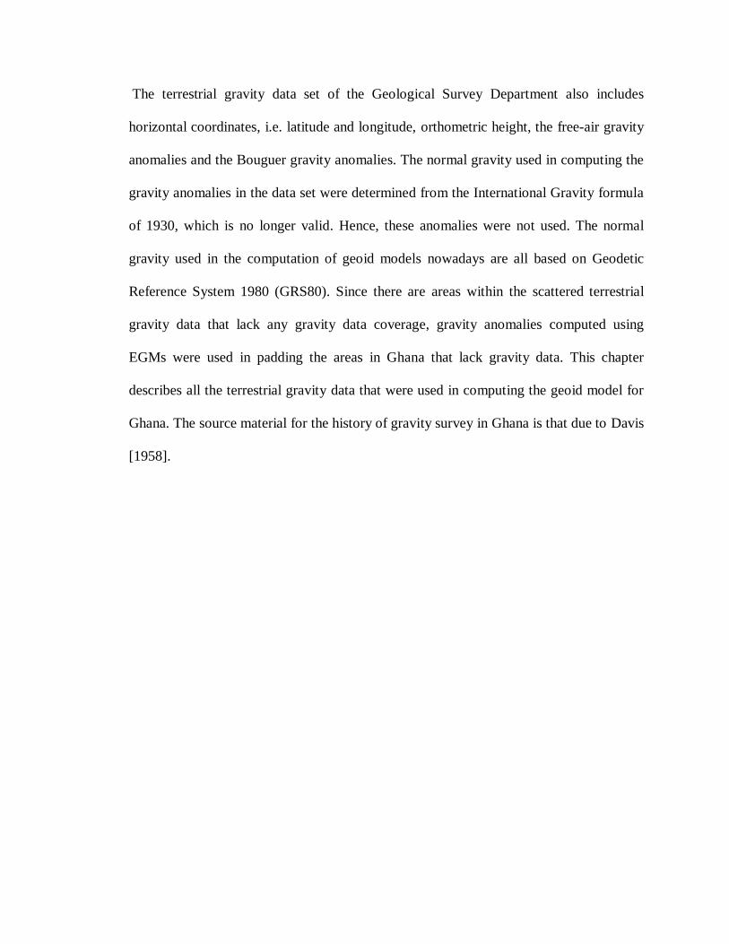
The terrestrial gravity data set of the Geological Survey Department also includes
horizontal coordinates, i.e. latitude and longitude, orthometric height, the free-air gravity
anomalies and the Bouguer gravity anomalies. The normal gravity used in computing the
gravity anomalies in the data set were determined from the International Gravity formula
of 1930, which is no longer valid. Hence, these anomalies were not used. The normal
gravity used in the computation of geoid models nowadays are all based on Geodetic
Reference System 1980 (GRS80). Since there are areas within the scattered terrestrial
gravity data that lack any gravity data coverage, gravity anomalies computed using
EGMs were used in padding the areas in Ghana that lack gravity data. This chapter
describes all the terrestrial gravity data that were used in computing the geoid model for
Ghana. The source material for the history of gravity survey in Ghana is that due to Davis
[1958].
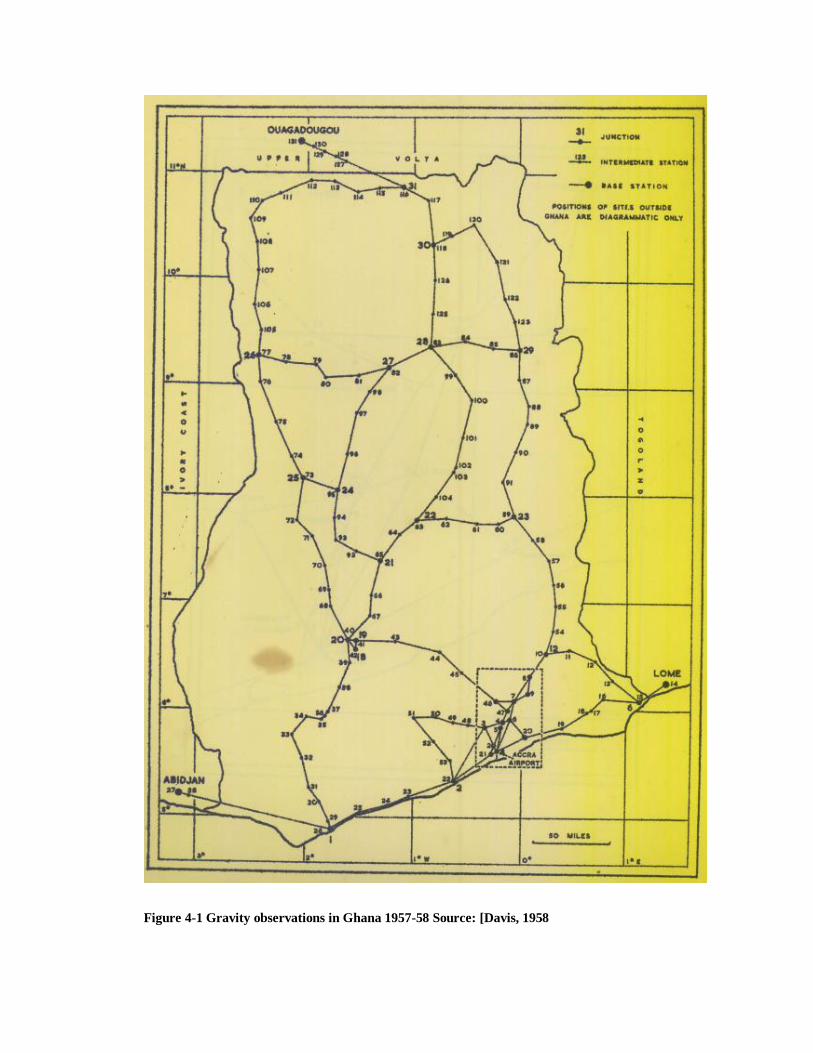
Figure 4-1 Gravity observations in Ghana 1957-58 Source: [Davis, 1958
4.2 Terrestrial gravity data in Ghana
The British Government in collaboration with Ghana Government carried out the first
gravity survey in Ghana between 1957 and 1958. This gravity survey work was part of
Ghana’s contribution to the international Geophysical Year program in 1957-58. This
program aimed to establish a worldwide network of known gravity values. Gravity
observations were made at 128 sites. The network of gravity observations was linked to
the Office de la Recherche Scientific et Technique Outre-Mer (ORSTOM) network of the
neighboring countries. Three sites in the (ORSTOM) network outside Ghana were used:
Abidjan (Ivory Coast), Lome (Togo) and Ouagadougou (Burkina Faso). The ORSTOM
network includes several pendulum stations such as Paris (France) and establishing a link
with these base stations will ensure that the Ghana network would be compatible with
local data. The value of gravity for each site was determined with an uncertainty of less
than 0.2 mGal. The Ghana network was also linked with the well-established gravity
network of the United Kingdom.
The standard deviations of the connection were all below 0.27 mGal and 70% of them
were below 0.05 mGal. The network is made up of 20 internal loops involving only the
connections and three other loops at the edge of the network involving the base stations
as well. The smallest miss closure is 0.01 mGal and the largest 0.34 mGal. Half of the
miss closure is less than 0.10 mgal. Ideally, the loops should be triangles or quadrilaterals
but owing to the lack of navigable roads, half the loops are many-sided polygons, some
with over 20 sides. The network was adjusted using least squares adjustment .method.
Since it was necessary to link the Ghanaian gravity network to the gravity network of the
neighboring countries, the calibration factor of the gravimeter used for the gravity survey
work was treated as unknown in the adjustment. A weight was assigned to each leg as a
measure of its reliability. The normal practice is to regard each leg as having equal
weight and thus, after the usual principle of combining standard deviations, each leg is
assigned a weight inversely proportional to the square root of the number of connections
constituting it, in manner similar to topographical survey. However due to the wide
spread of the individual standard deviation from nearly 0.00 to 0.27 mGal, it was felt the
leg containing many connections would be abnormally heavily weighted. The
compromise adopted was all connections having standard deviation from nearly 0.00
mGal or 0.01mGal are treated as if they had a standard deviation of 0.02 mGal. A
Pegasus computer made by Ferranti Ltd was used for the computation. The tripod height
allowance, i.e., the height of the gravimeter above ground was accounted for.
The ORSTOM network is based on the Potsdam system. However, a decision was made
to establish an independent link to the new network in Ghana. The sites occupied during
the linking from London Heathrow Airport were Rome Airport in Italy, Tripoli Airport in
Libya, Kano Airport in Nigeria and finally Accra Airport. The Geological Survey and
Museum (GSM), London supplied gravity values for the London Airport. Wollard
supplied the gravity values for Rome, Tripoli and Kano airports. The connections
between the stations are as follows:
1. London–Rome–London
2. Rome–Tripoli–Rome
3. Tripoli–Kano–Tripoli
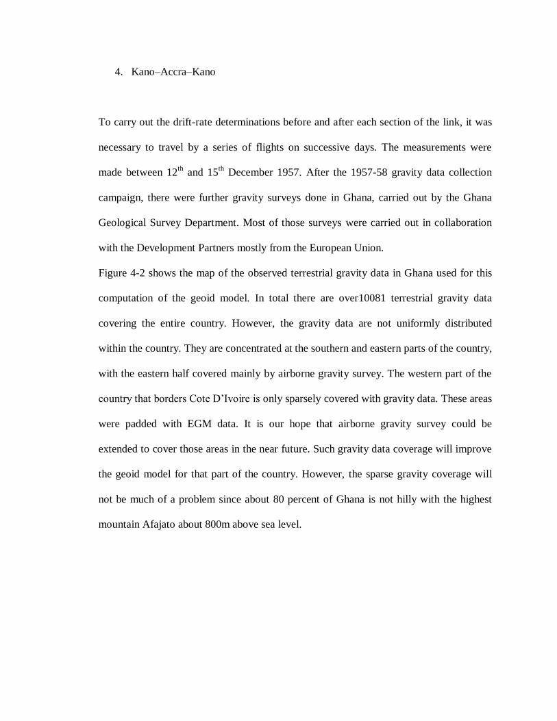
4. Kano–Accra–Kano
To carry out the drift-rate determinations before and after each section of the link, it was
necessary to travel by a series of flights on successive days. The measurements were
made between 12th
and 15th
December 1957. After the 1957-58 gravity data collection
campaign, there were further gravity surveys done in Ghana, carried out by the Ghana
Geological Survey Department. Most of those surveys were carried out in collaboration
with the Development Partners mostly from the European Union.
Figure 4-2 shows the map of the observed terrestrial gravity data in Ghana used for this
computation of the geoid model. In total there are over10081 terrestrial gravity data
covering the entire country. However, the gravity data are not uniformly distributed
within the country. They are concentrated at the southern and eastern parts of the country,
with the eastern half covered mainly by airborne gravity survey. The western part of the
country that borders Cote D’Ivoire is only sparsely covered with gravity data. These areas
were padded with EGM data. It is our hope that airborne gravity survey could be
extended to cover those areas in the near future. Such gravity data coverage will improve
the geoid model for that part of the country. However, the sparse gravity coverage will
not be much of a problem since about 80 percent of Ghana is not hilly with the highest
mountain Afajato about 800m above sea level.
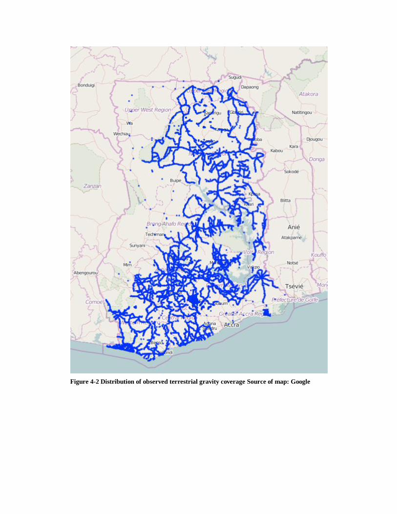
Figure 4-2 Distribution of observed terrestrial gravity coverage Source of map: Google
4.3 Computing the gravity anomalies and residual gravity anomalies
Equation 3.9 was used to compute gravity anomalies on the telluroid for all the 10081
gravity points in Ghana. Because of the sparse gravity data coverage of Ghana, a decision
was made to pad the areas in Ghana that lacked gravity data with data generated from
EGM08. The padding was carried out as follows:
1. A file containing list of latitude, longitude and orthometric height of the scattered
gravity data points from Ghana terrestrial gravity survey data were used as input
data to compute the gravity anomalies from the EGM. GrafLab a MATLAB
program was used to compute of the gravity anomalies [Bucha and Janák, 2013].
2. This was followed by a computation of residual gravity anomalies, which are the
difference between the terrestrial gravity anomalies and gravity anomalies from
the EGM08 i.e.
08EGMobservRES ggg
(4.1)
where RESg is the residual gravity anomaly, observg is the terrestrial surface
gravity anomaly, and 08EGMg is the gravity anomaly computed from the EGM08.
3. A plot of the residual anomalies (shown in Fig. 4.3) indicates that the residual anomalies
are normally distributed but not randomly distributed around the mean of zero and there
are outliers. Hence statistical test were computed and outliers were eliminated
4. The residual gravity anomalies were gridded. The SURFER Software with inverse
distance squared interpolation method was used for was used for gridding. The
residual anomalies were gridded at 5'5' intervals.
5. Three columns of the output file of the DTE computation, i.e. the latitude,
longitude, and heights (the DTE grid) were used as input data into the GrafLab
program to compute free-air gravity anomalies from EGM08. This DTE grid is
bounded by latitude 2ºS and 18ºN, and longitudes 10ºW and 8ºE
6. The free-air anomalies computed from the EGM08 were added to the residual
anomalies to obtain free-air gravity anomalies.
4.4 Statistical test for outliers
The accuracy of a computed geoid model depends on the quality of gravity data used in
the computation process. To ensure that the terrestrial gravity data used for computing the
geoid model is free of gross and systematic errors as much as possible, statistical test was
carried out on the residual gravity anomalies computed in Section 4.3. The aim of this
statistical test is for the detection of outliers. The assumption made was the residual
gravity values should be zero mean. The computation resulted in a mean of 1.947 mGal
and standard deviation of 5.706 mGal. A plot of the histogram of the residual is shown in
Fig 4.3. A 99.99% confidence interval for a two tail test was selected, and a normal test
of a single observation carried out. This resulted in a critical region of -12.774mGal< <
+16.668mGal. Thus, residual gravity anomalies below -12.774mGal and those above
+16.668mGal were rejected as outliers. Of the 10081 points terrestrial gravity data points,
117 terrestrial gravity points were rejected as outliers probably due to blunders.
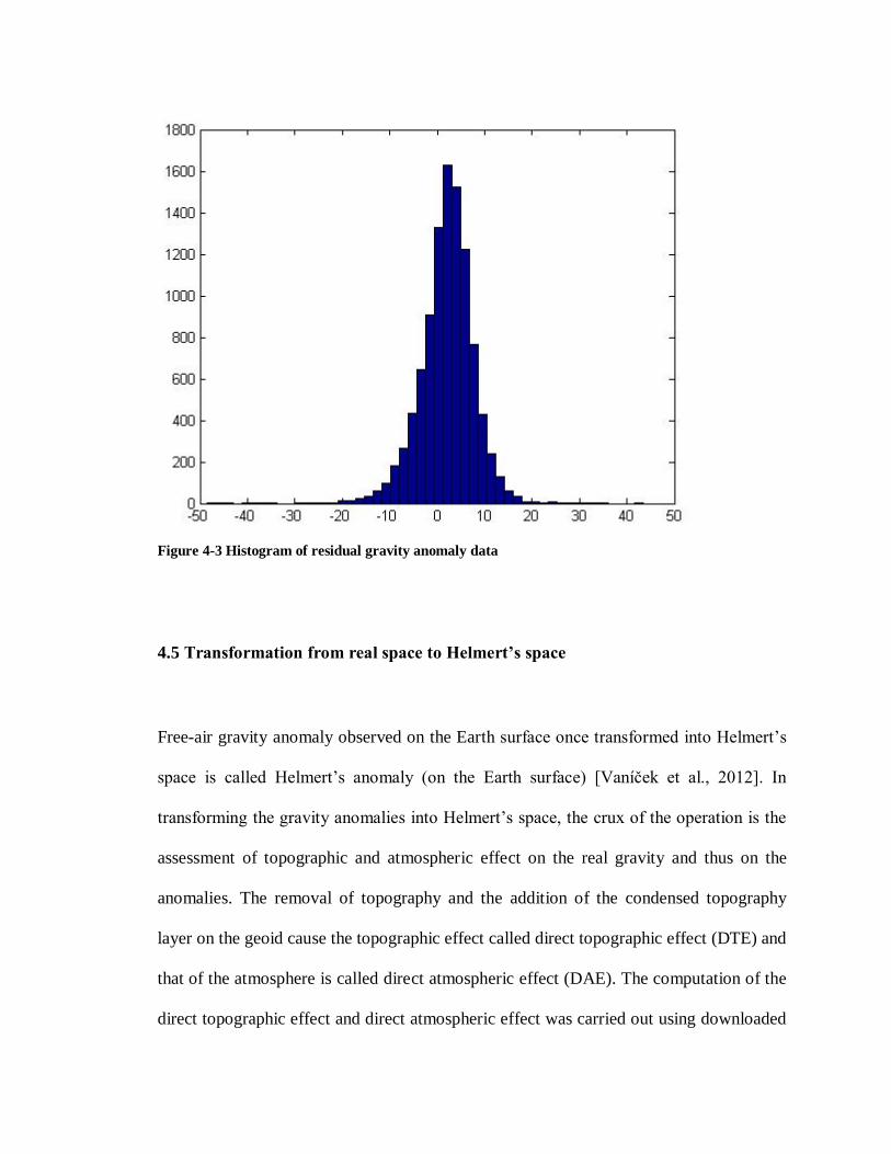
Figure 4-3 Histogram of residual gravity anomaly data
4.5 Transformation from real space to Helmert’s space
Free-air gravity anomaly observed on the Earth surface once transformed into Helmert’s
space is called Helmert’s anomaly (on the Earth surface) [Vaníček et al., 2012]. In
transforming the gravity anomalies into Helmert’s space, the crux of the operation is the
assessment of topographic and atmospheric effect on the real gravity and thus on the
anomalies. The removal of topography and the addition of the condensed topography
layer on the geoid cause the topographic effect called direct topographic effect (DTE) and
that of the atmosphere is called direct atmospheric effect (DAE). The computation of the
direct topographic effect and direct atmospheric effect was carried out using downloaded
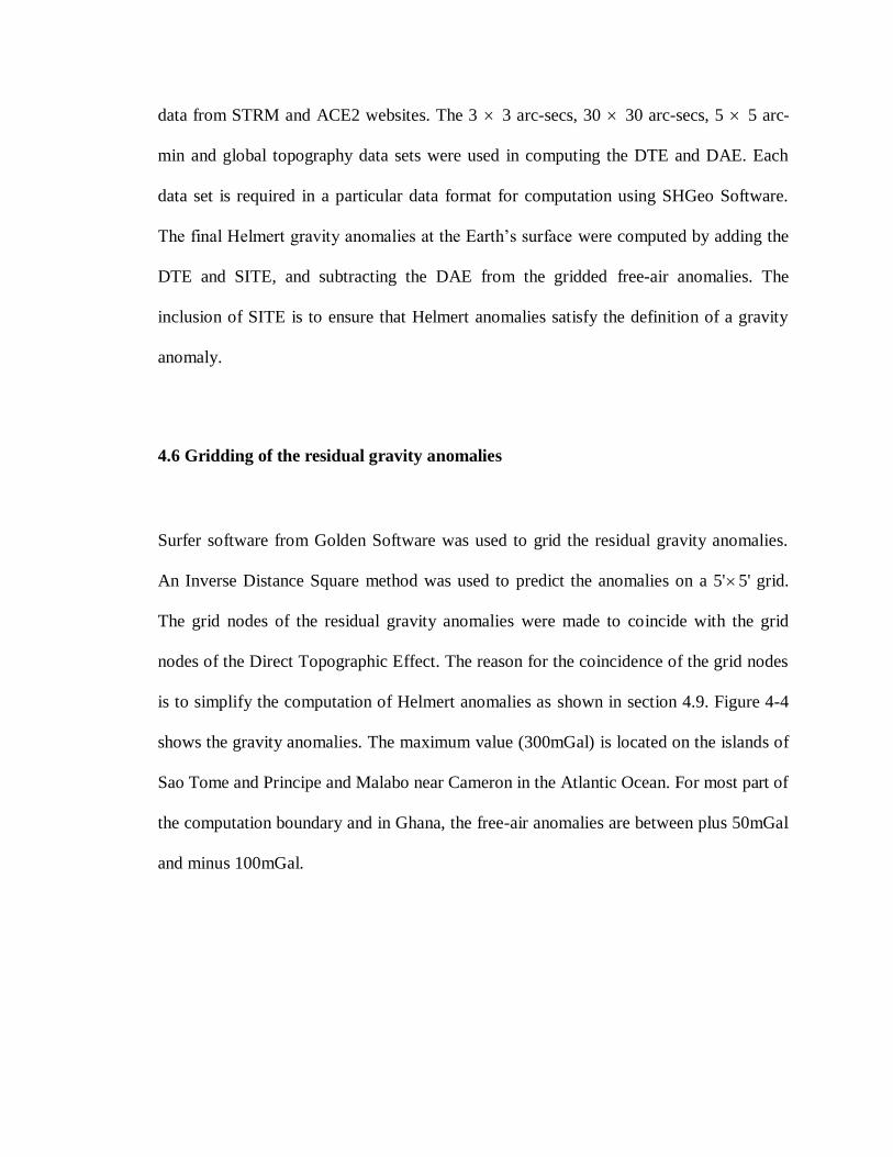
data from STRM and ACE2 websites. The 3 3 arc-secs, 30 30 arc-secs, 5 5 arc-
min and global topography data sets were used in computing the DTE and DAE. Each
data set is required in a particular data format for computation using SHGeo Software.
The final Helmert gravity anomalies at the Earth’s surface were computed by adding the
DTE and SITE, and subtracting the DAE from the gridded free-air anomalies. The
inclusion of SITE is to ensure that Helmert anomalies satisfy the definition of a gravity
anomaly.
4.6 Gridding of the residual gravity anomalies
Surfer software from Golden Software was used to grid the residual gravity anomalies.
An Inverse Distance Square method was used to predict the anomalies on a 5'5' grid.
The grid nodes of the residual gravity anomalies were made to coincide with the grid
nodes of the Direct Topographic Effect. The reason for the coincidence of the grid nodes
is to simplify the computation of Helmert anomalies as shown in section 4.9. Figure 4-4
shows the gravity anomalies. The maximum value (300mGal) is located on the islands of
Sao Tome and Principe and Malabo near Cameron in the Atlantic Ocean. For most part of
the computation boundary and in Ghana, the free-air anomalies are between plus 50mGal
and minus 100mGal.
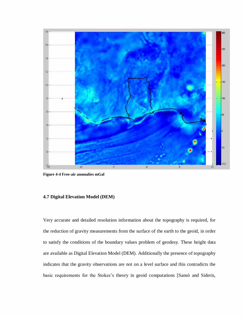
Figure 4-4 Free-air anomalies mGal
4.7 Digital Elevation Model (DEM)
Very accurate and detailed resolution information about the topography is required, for
the reduction of gravity measurements from the surface of the earth to the geoid, in order
to satisfy the conditions of the boundary values problem of geodesy. These height data
are available as Digital Elevation Model (DEM). Additionally the presence of topography
indicates that the gravity observations are not on a level surface and this contradicts the
basic requirements for the Stokes’s theory in geoid computations [Sansò and Sideris,
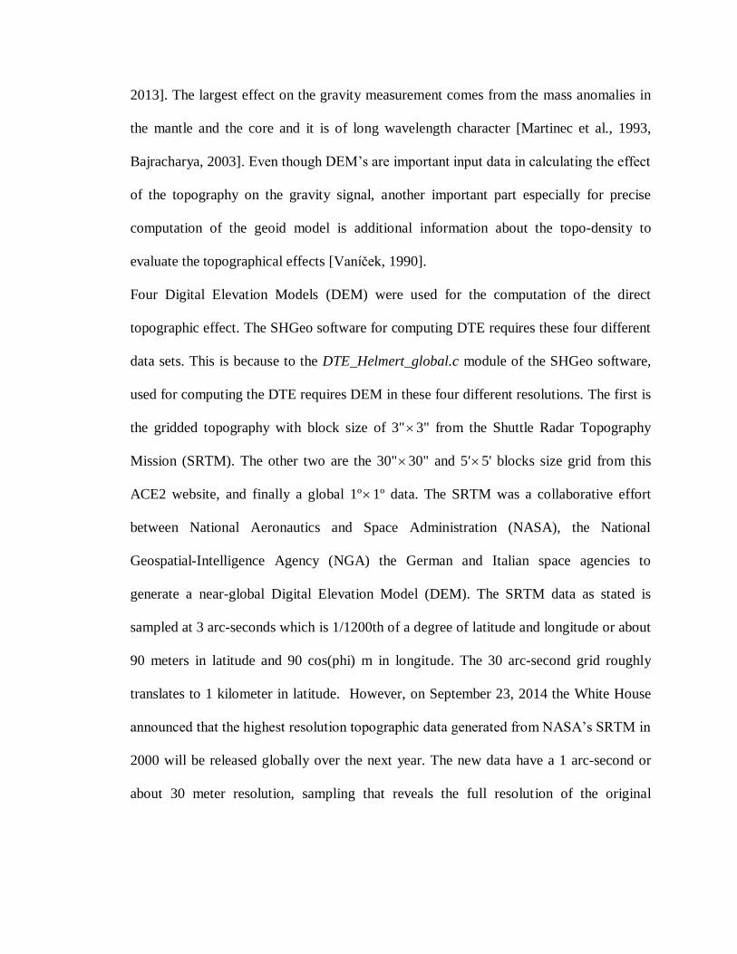
2013]. The largest effect on the gravity measurement comes from the mass anomalies in
the mantle and the core and it is of long wavelength character [Martinec et al., 1993,
Bajracharya, 2003]. Even though DEM’s are important input data in calculating the effect
of the topography on the gravity signal, another important part especially for precise
computation of the geoid model is additional information about the topo-density to
evaluate the topographical effects [Vaníček, 1990].
Four Digital Elevation Models (DEM) were used for the computation of the direct
topographic effect. The SHGeo software for computing DTE requires these four different
data sets. This is because to the DTE_Helmert_global.c module of the SHGeo software,
used for computing the DTE requires DEM in these four different resolutions. The first is
the gridded topography with block size of 3"3" from the Shuttle Radar Topography
Mission (SRTM). The other two are the 30"30" and 5'5' blocks size grid from this
ACE2 website, and finally a global 1º1º data. The SRTM was a collaborative effort
between National Aeronautics and Space Administration (NASA), the National
Geospatial-Intelligence Agency (NGA) the German and Italian space agencies to
generate a near-global Digital Elevation Model (DEM). The SRTM data as stated is
sampled at 3 arc-seconds which is 1/1200th of a degree of latitude and longitude or about
90 meters in latitude and 90 cos(phi) m in longitude. The 30 arc-second grid roughly
translates to 1 kilometer in latitude. However, on September 23, 2014 the White House
announced that the highest resolution topographic data generated from NASA’s SRTM in
2000 will be released globally over the next year. The new data have a 1 arc-second or
about 30 meter resolution, sampling that reveals the full resolution of the original
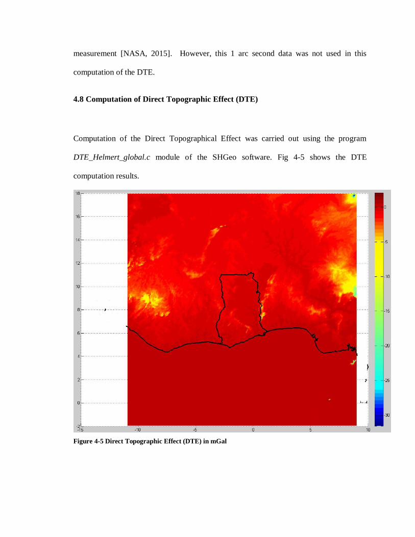
measurement [NASA, 2015]. However, this 1 arc second data was not used in this
computation of the DTE.
4.8 Computation of Direct Topographic Effect (DTE)
Computation of the Direct Topographical Effect was carried out using the program
DTE_Helmert_global.c module of the SHGeo software. Fig 4-5 shows the DTE
computation results.
Figure 4-5 Direct Topographic Effect (DTE) in mGal
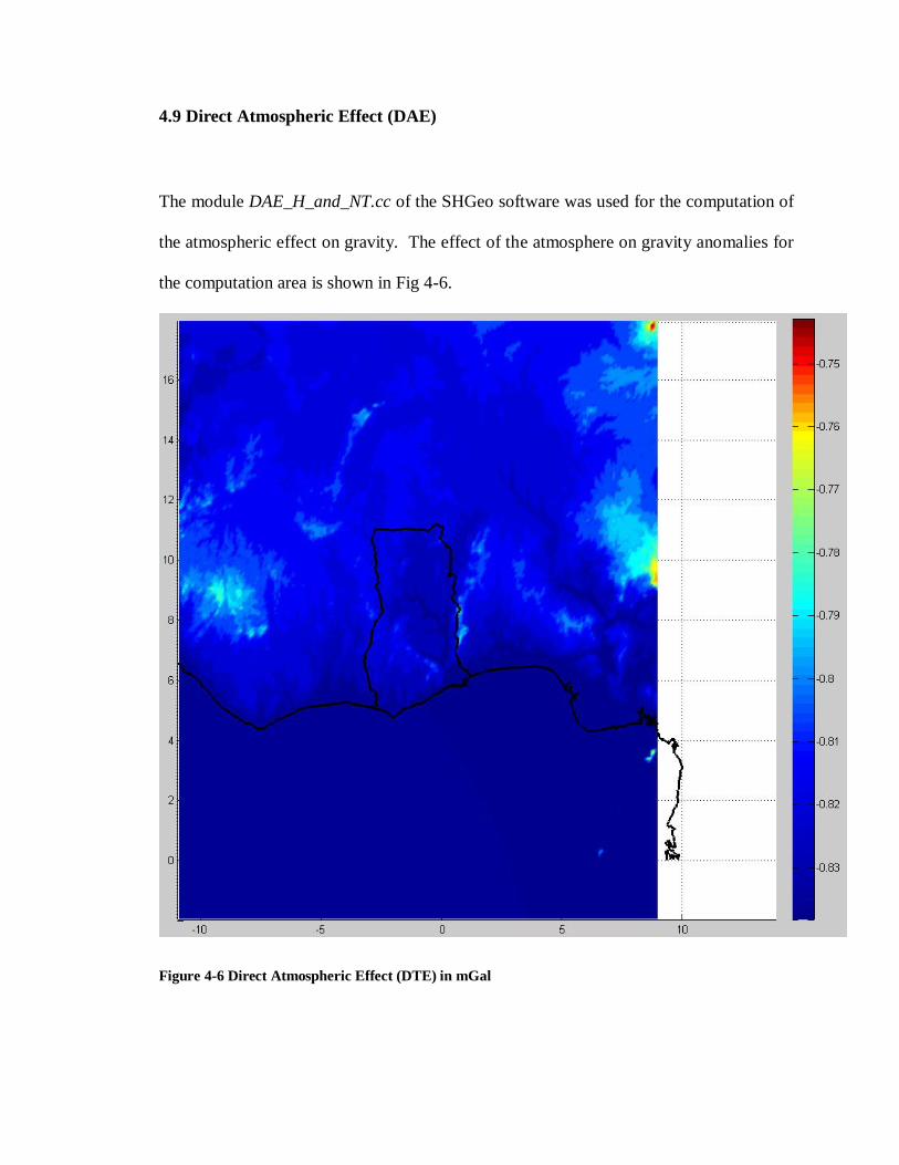
4.9 Direct Atmospheric Effect (DAE)
The module DAE_H_and_NT.cc of the SHGeo software was used for the computation of
the atmospheric effect on gravity. The effect of the atmosphere on gravity anomalies for
the computation area is shown in Fig 4-6.
Figure 4-6 Direct Atmospheric Effect (DTE) in mGal
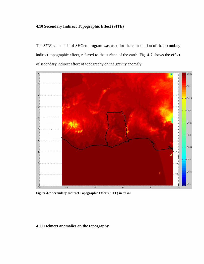
4.10 Secondary Indirect Topographic Effect (SITE)
The SITE.cc module of SHGeo program was used for the computation of the secondary
indirect topographic effect, referred to the surface of the earth. Fig. 4-7 shows the effect
of secondary indirect effect of topography on the gravity anomaly.
Figure 4-7 Secondary Indirect Topographic Effect (SITE) in mGal
4.11 Helmert anomalies on the topography
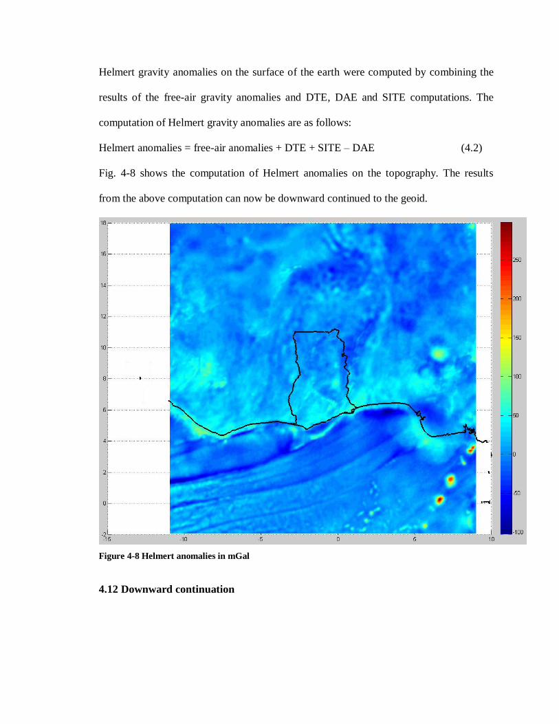
Helmert gravity anomalies on the surface of the earth were computed by combining the
results of the free-air gravity anomalies and DTE, DAE and SITE computations. The
computation of Helmert gravity anomalies are as follows:
Helmert anomalies = free-air anomalies + DTE + SITE – DAE (4.2)
Fig. 4-8 shows the computation of Helmert anomalies on the topography. The results
from the above computation can now be downward continued to the geoid.
Figure 4-8 Helmert anomalies in mGal
4.12 Downward continuation
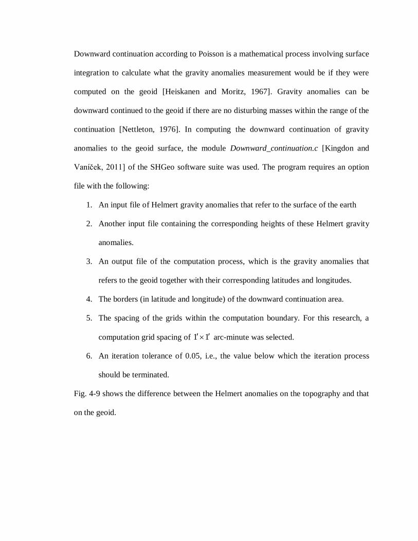
Downward continuation according to Poisson is a mathematical process involving surface
integration to calculate what the gravity anomalies measurement would be if they were
computed on the geoid [Heiskanen and Moritz, 1967]. Gravity anomalies can be
downward continued to the geoid if there are no disturbing masses within the range of the
continuation [Nettleton, 1976]. In computing the downward continuation of gravity
anomalies to the geoid surface, the module Downward_continuation.c [Kingdon and
Vaníček, 2011] of the SHGeo software suite was used. The program requires an option
file with the following:
1. An input file of Helmert gravity anomalies that refer to the surface of the earth
2. Another input file containing the corresponding heights of these Helmert gravity
anomalies.
3. An output file of the computation process, which is the gravity anomalies that
refers to the geoid together with their corresponding latitudes and longitudes.
4. The borders (in latitude and longitude) of the downward continuation area.
5. The spacing of the grids within the computation boundary. For this research, a
computation grid spacing of 11 arc-minute was selected.
6. An iteration tolerance of 0.05, i.e., the value below which the iteration process
should be terminated.
Fig. 4-9 shows the difference between the Helmert anomalies on the topography and that
on the geoid.
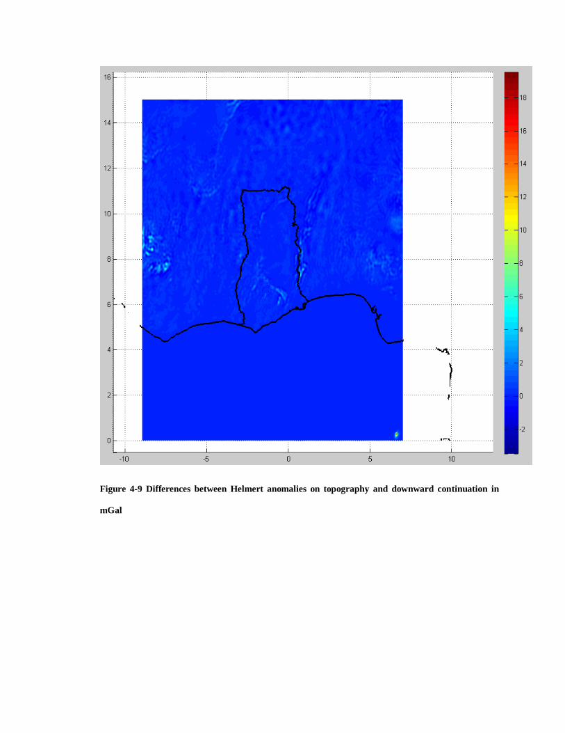
Figure 4-9 Differences between Helmert anomalies on topography and downward continuation in
mGal
4.13 Reference Field
The long-wavelength part of the gravity signal predicted from the EGM08 up to degree
90 is removed from the Helmert gravity anomalies on the geoid. This removes the
unreliable low-frequency part of the terrestrial gravity data and indicates the limits of the
integration i.e. the o20 of integration cap around the computation points. The degree
and order 90 of EGM08 was tested and found to give relatively reliable results.
Computation of the reference field was carried out using the program
Reference_field_2001_HighDegree.f in the SHGeo package. The reference field is shown
Fig 4-10.
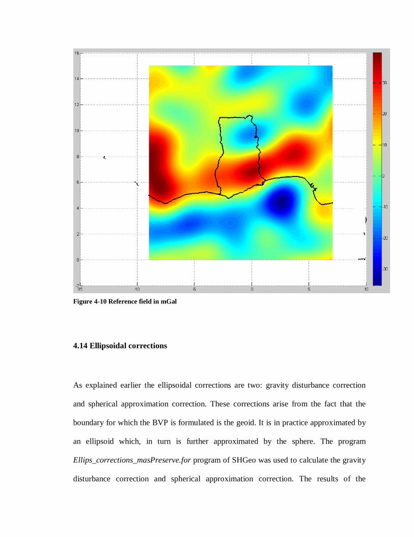
Figure 4-10 Reference field in mGal
4.14 Ellipsoidal corrections
As explained earlier the ellipsoidal corrections are two: gravity disturbance correction
and spherical approximation correction. These corrections arise from the fact that the
boundary for which the BVP is formulated is the geoid. It is in practice approximated by
an ellipsoid which, in turn is further approximated by the sphere. The program
Ellips_corrections_masPreserve.for program of SHGeo was used to calculate the gravity
disturbance correction and spherical approximation correction. The results of the
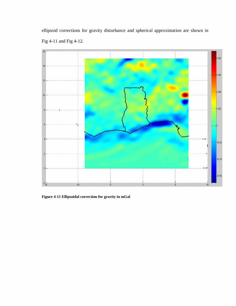
ellipsoid corrections for gravity disturbance and spherical approximation are shown in
Fig 4-11 and Fig 4-12.
Figure 4-11 Ellipsoidal correction for gravity in mGal
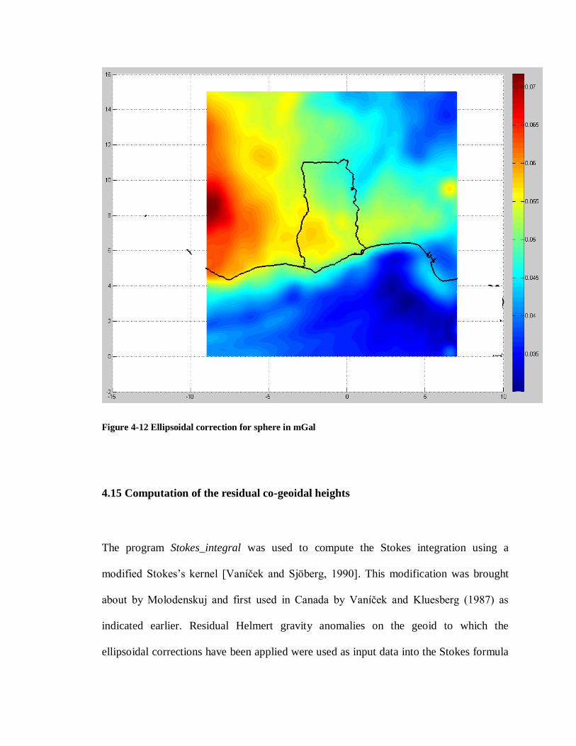
Figure 4-12 Ellipsoidal correction for sphere in mGal
4.15 Computation of the residual co-geoidal heights
The program Stokes_integral was used to compute the Stokes integration using a
modified Stokes’s kernel [Vaníček and Sjöberg, 1990]. This modification was brought
about by Molodenskuj and first used in Canada by Vaníček and Kluesberg (1987) as
indicated earlier. Residual Helmert gravity anomalies on the geoid to which the
ellipsoidal corrections have been applied were used as input data into the Stokes formula
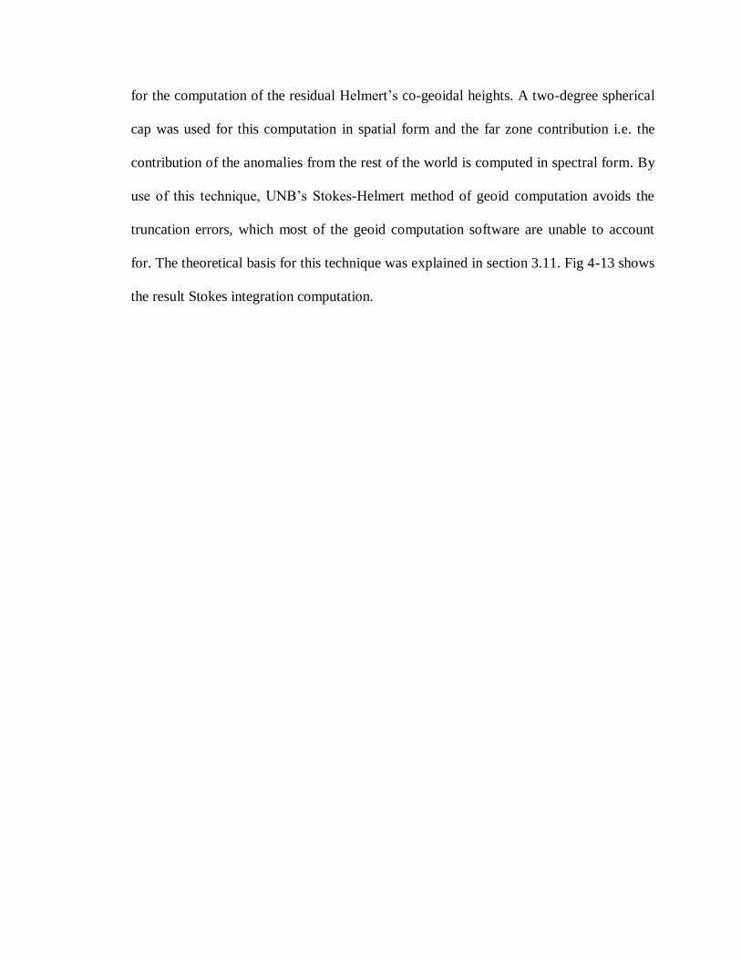
for the computation of the residual Helmert’s co-geoidal heights. A two-degree spherical
cap was used for this computation in spatial form and the far zone contribution i.e. the
contribution of the anomalies from the rest of the world is computed in spectral form. By
use of this technique, UNB’s Stokes-Helmert method of geoid computation avoids the
truncation errors, which most of the geoid computation software are unable to account
for. The theoretical basis for this technique was explained in section 3.11. Fig 4-13 shows
the result Stokes integration computation.
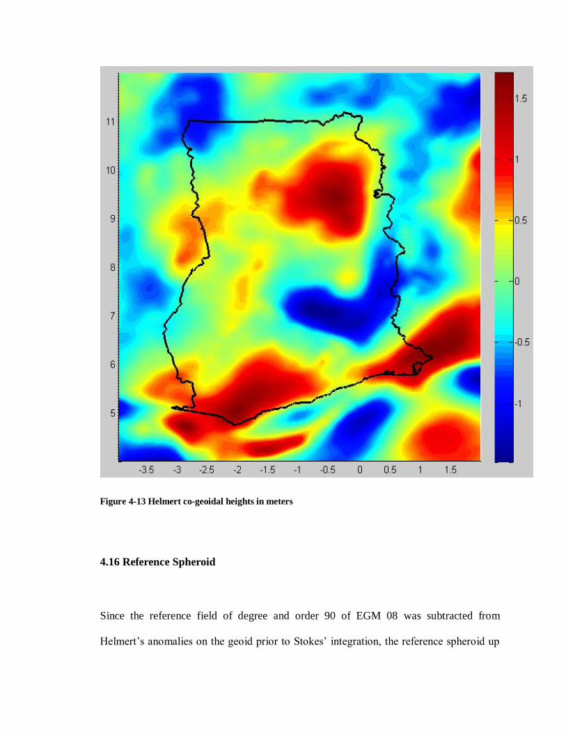
Figure 4-13 Helmert co-geoidal heights in meters
4.16 Reference Spheroid
Since the reference field of degree and order 90 of EGM 08 was subtracted from
Helmert’s anomalies on the geoid prior to Stokes’ integration, the reference spheroid up
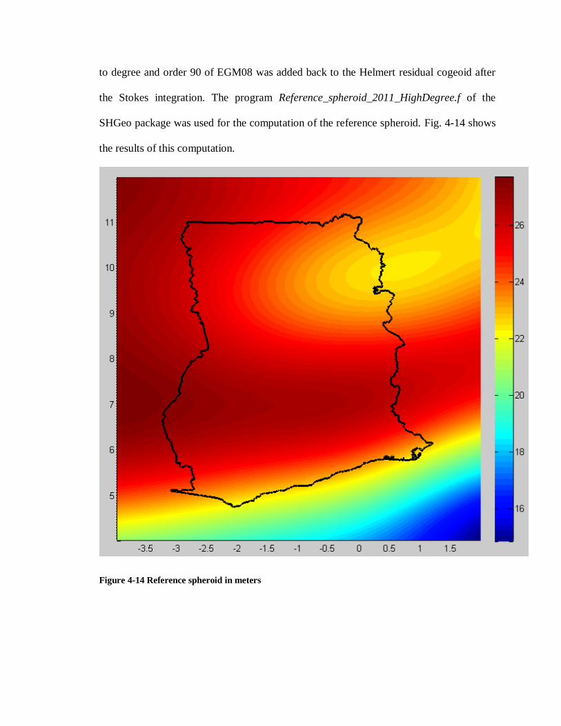
to degree and order 90 of EGM08 was added back to the Helmert residual cogeoid after
the Stokes integration. The program Reference_spheroid_2011_HighDegree.f of the
SHGeo package was used for the computation of the reference spheroid. Fig. 4-14 shows
the results of this computation.
Figure 4-14 Reference spheroid in meters
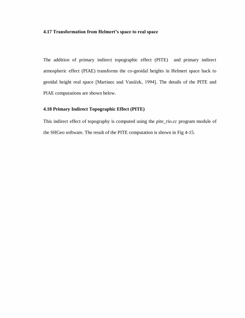
4.17 Transformation from Helmert’s space to real space
The addition of primary indirect topographic effect (PITE) and primary indirect
atmospheric effect (PIAE) transforms the co-geoidal heights in Helmert space back to
geoidal height real space [Martinec and Vaníček, 1994]. The details of the PITE and
PIAE computations are shown below.
4.18 Primary Indirect Topographic Effect (PITE)
This indirect effect of topography is computed using the pite_rio.cc program module of
the SHGeo software. The result of the PITE computation is shown in Fig 4-15.
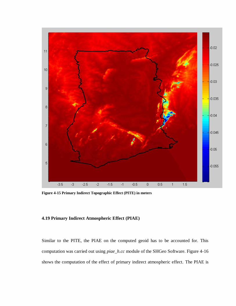
Figure 4-15 Primary Indirect Topographic Effect (PITE) in meters
4.19 Primary Indirect Atmospheric Effect (PIAE)
Similar to the PITE, the PIAE on the computed geoid has to be accounted for. This
computation was carried out using piae_h.cc module of the SHGeo Software. Figure 4-16
shows the computation of the effect of primary indirect atmospheric effect. The PIAE is
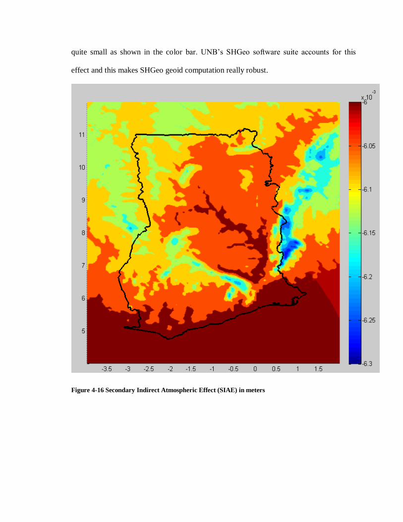
quite small as shown in the color bar. UNB’s SHGeo software suite accounts for this
effect and this makes SHGeo geoid computation really robust.
Figure 4-16 Secondary Indirect Atmospheric Effect (SIAE) in meters
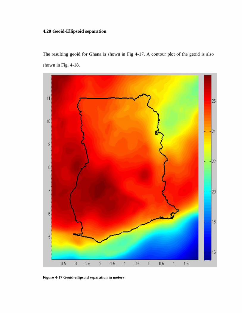
4.20 Geoid-Ellipsoid separation
The resulting geoid for Ghana is shown in Fig 4-17. A contour plot of the geoid is also
shown in Fig. 4-18.
Figure 4-17 Geoid-ellipsoid separation in meters
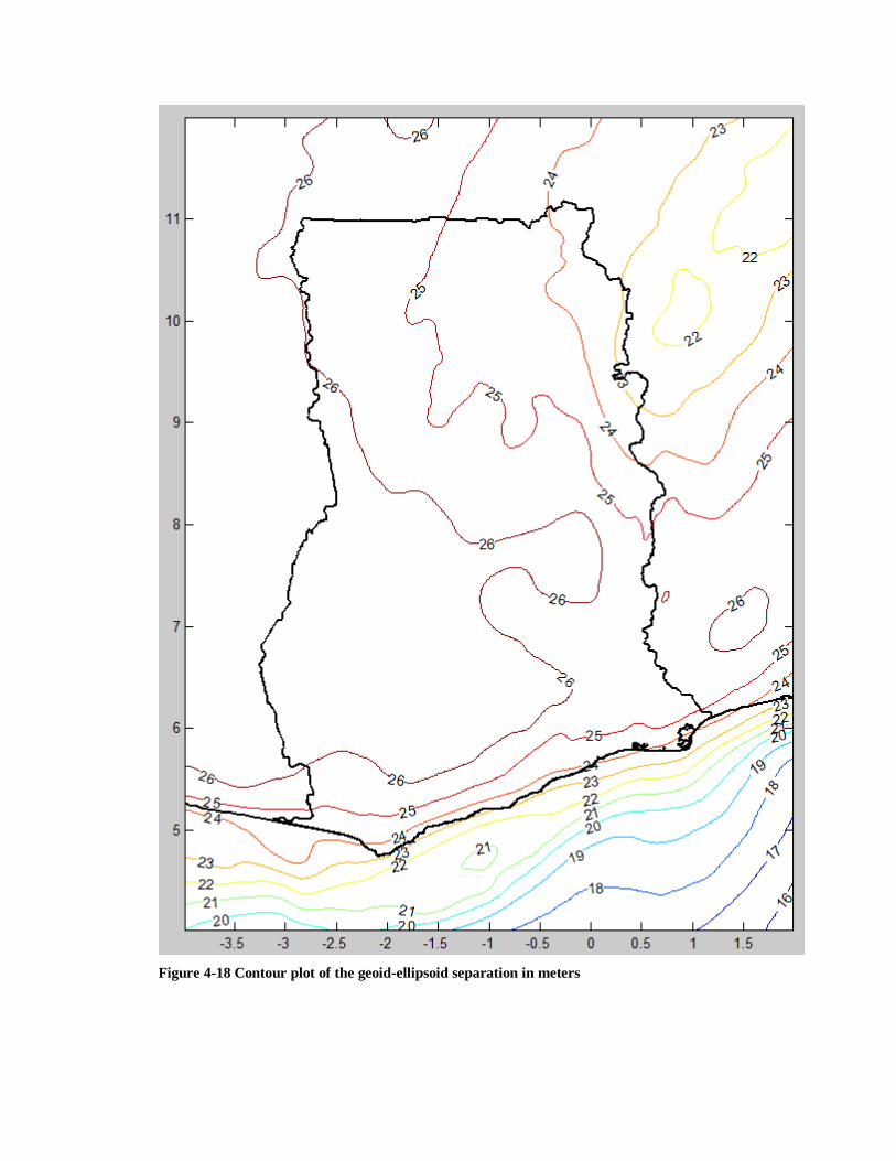
Figure 4-18 Contour plot of the geoid-ellipsoid separation in meters
4.21 GNSS/trigonometric-levelling data
Measurements from GNSS receivers provide geodetic heights, which are heights referred
from the surface of referenced ellipsoid to the points of interest and measured along the
normal of the ellipsoid. Orthometric height is referenced from the geoid to the point of
interest and is measured along the plumbline. Orthometric heights are obtained mainly by
spirit levelling and to a less degree of accuracy by trigonometric levelling. Equation 4.3
below shows the relationship between the geoidal height, geodetic height and orthometric
as:
HhN (4.3)
where N is the geoidal height, h is the geodetic height and H is the orthometric height.
GNSS/trigonometric-leveling is a technique based on the use of the above equation, i.e.,
N = h–H. If the geodetic height h is obtained from GNSS measurements, and the
orthometric height H is available from levelling, their differences can be compared
against the computed N.
GNSS/trigonometric-levelling technique can be used to assess the accuracy of the
computed gravimetric geoid model and vise-versa. Unfortunately, orthometric heights
obtained from spirit levelling, together with its GNSS data, are not readily available in
Ghana as at the time of testing this geoid model. However, less accurate trigonometric
heights can be extracted from the old triangulation network established by the British
from 1924 to 1926 [Clendinning, 1926]. These trigonometric heights were provided by
the examination section of the Survey and Mapping Division of the Lands Commission.
These orthometric heights were computed from trigonometric levelling data during the
triangulation of the then Gold Coast and are thought to have generally a standard
deviation of about 25cm [Clark and Clendinning, 1923].
The total number of such points that can be used for the assessment of the Ghanaian
gravimetric geoid model is 13. The 13 points covers mainly the southern portions of the
country usually referred to as the ―golden triangle‖. There may be inconsistencies in the
computation of the trigonometrical heights since the computations were not adjusted
homogeneously. GNSS determined geodetic heights were observed on these
trigonometric points during the first phase of the Land Administration project in 2007.
Each point was observed for a minimum of 12 hours.
As shown in the table below, the differences between GNSS/trigonometric-levelling
determined geoidal heights and those determined in our computation ranges from -0.958
m to 0.973 m. These relatively large differences are due to the errors in the elevation
values from the trigonometric levelling network, since the network has not been adjusted
homogenously and additionally only has thirteen points. These points are located on high
mountains, see Figs. 4.19 and 4.20. As a result, these trigonometrically determine
heights are not good enough to use in evaluating geoid model accuracy. Height
determined from precise levelling will be a better measure of assessing the accuracy of
the geoid model. Again trigonometrically determined heights suffer from refraction
correction errors, which are very significant (see later). From table 1 and table 2, it can
be seen that the points with higher elevations have relatively higher differences. It is
worth mentioning that the computation of the geoid model (if carried out using a criterion
that made residual anomalies less than -10 mgal and that greater than +10 mgal as
outliers) produces only slightly better relatively to GNSS/trigonometric-levelling
differences. This indicates that the large differences in the assessment of the accuracy of
the computed geoid model are due to the errors in the trigonometric levelling and not in
the gravity data. Table 2 shows the results of this computation. Figure 4-19 shows the
locations of the trigonometric points used for assessing the geoid model. An enlarged
form of these locations is in figure 4-20. One may also check the accuracy of the
computed geoid model by using GOCE TIM5 EGM up to degree and order (d/o) 200
combined by EGM2008 from d/o 201 to d/o 2190.
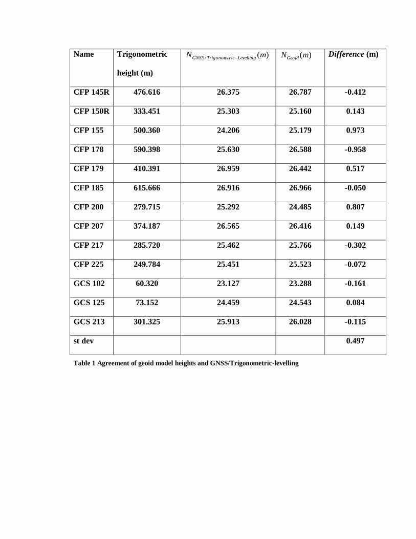
Name Trigonometric
height (m)
)(/ mN LevellingricTrigonometGNSS )(mNGeoid Difference (m)
CFP 145R 476.616 26.375 26.787 -0.412
CFP 150R 333.451 25.303 25.160 0.143
CFP 155 500.360 24.206 25.179 0.973
CFP 178 590.398 25.630 26.588 -0.958
CFP 179 410.391 26.959 26.442 0.517
CFP 185 615.666 26.916 26.966 -0.050
CFP 200 279.715 25.292 24.485 0.807
CFP 207 374.187 26.565 26.416 0.149
CFP 217 285.720 25.462 25.766 -0.302
CFP 225 249.784 25.451 25.523 -0.072
GCS 102 60.320 23.127 23.288 -0.161
GCS 125 73.152 24.459 24.543 0.084
GCS 213 301.325 25.913 26.028 -0.115
st dev 0.497
Table 1 Agreement of geoid model heights and GNSS/Trigonometric-levelling
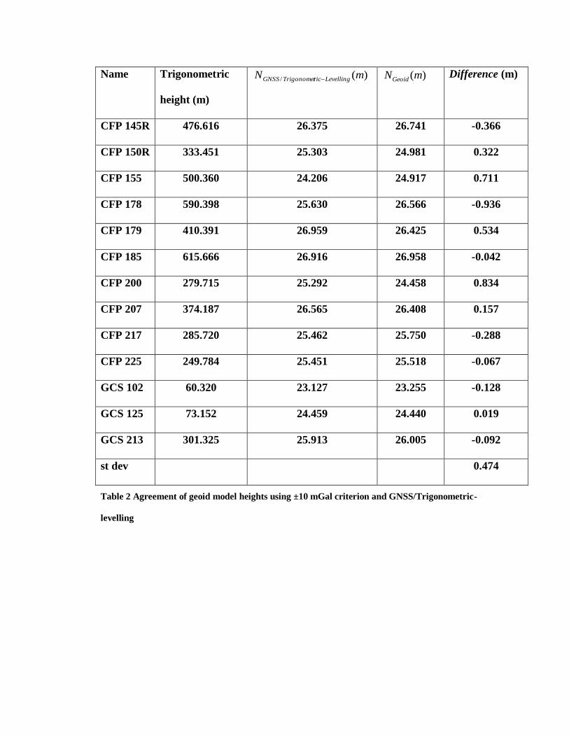
Name Trigonometric
height (m)
)(/ mN LevellingricTrigonometGNSS )(mNGeoid Difference (m)
CFP 145R 476.616 26.375 26.741 -0.366
CFP 150R 333.451 25.303 24.981 0.322
CFP 155 500.360 24.206 24.917 0.711
CFP 178 590.398 25.630 26.566 -0.936
CFP 179 410.391 26.959 26.425 0.534
CFP 185 615.666 26.916 26.958 -0.042
CFP 200 279.715 25.292 24.458 0.834
CFP 207 374.187 26.565 26.408 0.157
CFP 217 285.720 25.462 25.750 -0.288
CFP 225 249.784 25.451 25.518 -0.067
GCS 102 60.320 23.127 23.255 -0.128
GCS 125 73.152 24.459 24.440 0.019
GCS 213 301.325 25.913 26.005 -0.092
st dev 0.474
Table 2 Agreement of geoid model heights using ±10 mGal criterion and GNSS/Trigonometric-
levelling
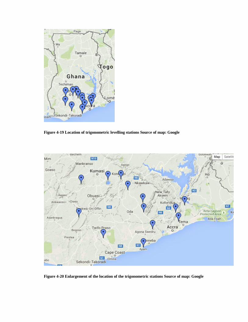
Figure 4-19 Location of trigonometric levelling stations Source of map: Google
Figure 4-20 Enlargement of the location of the trigonometric stations Source of map: Google
I think I did pretty well, considering I started out with nothing but a bunch of blank
paper.
Steve Martin
Chapter 5. Conclusions and recommendation
5.1 Conclusion
This thesis aims to compute gravimetric geoid of Ghana using terrestrial gravity data
covering the entire country. Such an undertaking is very difficult since Ghana is a
developing country with sparse gravity data coverage and a lack of information regarding
the quality of the gravity data. Additionally, this is the first time a geoid model has been
computed in Ghana. It is worth mentioning that even though it has been the aim of
geodesists in Africa to compute a geoid model for the entire continent, this has remained
on the drawing board for quite some time now [Combrinck et al., 2003].
The Stokes-Helmert approach in geoid computation has been used to compute the geoid
model of Ghana. This method was selected because it does not suffer from truncation
errors when computing the Stokes integration- a problem which most of the geoid
computation software are unable to handle effectively. This geoid model of Ghana is
available on a regular 11 grid over an area bounded by latitudes 4ºN and 12ºN and
longitudes 4ºW and 2ºE.
An important contribution of this research is the conversion of all the terrestrial gravity
data held by the Geological Survey Department to Geodetic Reference System 1980
(GRS80) and the elimination of duplicate gravity data from the database. The original
gravity anomalies were computed using the 1930 International gravity formula, which is
no longer valid. An attempt was made to contact BGI and GETECH for any additional
gravity data to improve the accuracy of the geoid model. These attempts met failures.
This research used the publicly available 3" STRM DEM since there is lack of high
resolution photogrammetric based DEM covering the entire country. In addition, EGM08
was selected and used among the wide range of EGMs because it were tested and prove
satisfactory accurate. EGM08 and STRM-DEM have been used to fill the gaps in sparse
gravity data coverage and the absence of a national DEM.
Statistical techniques were used for detection of outliers in the gravity data set prior to
gridding. This check on the gravity data led to the exclusion of 117 gravity
measurements. GPS/trigonometric levelling data was used to access the accuracy of the
computed geoid model. The standard deviation of the differences between the computed
geoid model and 13 GPS/trigonometric levelling data is estimated to 0.497m. Due to the
presence of systematic errors in the observation and adjustment of the GPS/trigonometric
levelling and gravity data, this assessment will not yield a true reflection of the accuracy
of the geoid model. Furthermore, a better way to assess the accuracy of the computed
geoid model is to use GPS/levelling data. The precise level data in Ghana have not been
computed and adjusted homogenously. Furthermore, if any precise level data is available,
there is the need to carry out GNSS observations on these bench marks before they can be
used to assess this computed geoid model. Absence of such data made it impossible to
really assess the accuracy of the first computed Ghanaian gravimetric geoid model.
5.2 Limitations of this research
1. As is characteristic of almost all geoid computation software that uses gridded data,
they are unable to compute the standard deviation of the positions outside the grid
points. This results in difficulties when comparing heights estimated from geoid
models with heights from bench marks since the bench marks are not located at the
gridded points used in the geoid computation.
2. There were issues with the quality of the gravity data used in the modelling of the
geoid. As can be found in most countries in the world, the main application of gravity
data is for mineral prospecting and not for geodetic purposes. Accordingly, Meta data
about the gravity data, such as the gravimeter used in acquiring, the accuracy of the
gravity measurement, positional accuracy and field procedures adopted during data
acquisition are usually missing. The quality of such Meta data will definitely affect
geoid model computed.
3. Use of a single density model value of 2.67g/cm3 will introduce biases in the
computed model. An accurate geoid model should account for the density variation
within the topography. Currently Ghana does not have a topographic laterally varying
density model. However, these biases will not be significant since the terrain in
Ghana is relatively low lying.
4. The lack of a national DEM also had an impact on the accuracy of topographic
reduction. Additionally, the sparse gravity data coverage especially at the western
part of Ghana will most likely affect the accuracy of the geoid model in that part of
Ghana since those areas were padded with EGM08 gravity data.
5. The absence of leveled height data reduced significantly the ability to test the
accuracy of the computed geoid model.
6. The lack of uniformly distributed gravity data which covers the entire country also
impose a limit on the accuracy which could be achieve in computing the geoid model.
5.3 Recommendation
In computing the gravimetric geoid model of Ghana, a major constraint is the lack of
gravity data from western part of Ghana, the neighboring countries and in the sea. As
pointed out in the theory of geoid computations, there is the need for gravity anomaly
data to at least a 3º distance from the country borders. Since there are no gravity data for
the areas surrounding Ghana’s borders, those empty blocks were padded with data
generated from EGM08. This 3º requirement in geoid computation implies all the
neighboring countries will also require data from Ghana in order to compute their geoids.
It is recommended that geodesists in the sub-region should combine their efforts by
making available terrestrial gravity data sets from their respective countries to compute a
geoid models for the entire West Africa sub-region.
With gravity data distribution of one gravity data per 23 sq. km, it is evident that
centimeter geoid accuracy is currently not reachable. There are large areas especially in
the northwestern part of the Ghana that do not have gravity data coverage. Lack of funds
and logistics are some of the drawbacks for the lack of gravity measurements in those
areas. It is recommended that the government should carry out airborne gravity survey in
those areas in order to increase the quality and quantity of gravity data.
Since the central to the eastern portion of the country right into the Republic of Togo
have been covered with airborne gravity data, it is recommended that future computation
of the geoid should include these gravity data. Combining terrestrial and airborne gravity
data will require specialized software since downward continuation of airborne gravity
requires different processing. This inclusion should lead to an improve accuracy of the
modelled geoid.
To evaluate the gravimetric geoid model will require a dense network of high quality
GPS/levelling points well distributed throughout the country. As an interim measure,
assessment of this computed geoid model should continue throughout the country using
levelling/benchmark information available. This will increase user confidence in this
computed geoid model. This will ultimately lead to the identification of regions within
the geoid model where there is the need for further improvement.
To assess the accuracy of a geoid model and EGM requires well distributed
GPS/Levelling data. Such data must cover the entire area of the geoid model. Impartial
results in this assessment will require a network of Fundamental Bench Marks (FBM),
which have been correctly reduced. These FBMs together with the other bench marks
should be adjusted homogenously and their quality (standard deviations) stated. The
situation in Ghana is quite different. The FBMs are mostly located in the Regional
Capitals. Furthermore, the entire spirit levelling network has not been adjusted
homogenously. It is also worth mentioning that quite a few of the bench marks are
located at trigonometric points. These trigonometric points are the vertices of
triangulation network carried out by the British in the early 1920s. As a result, their
standard deviations are unknown making it difficult to assess the quality of the geoid
model. It is therefore important that the Geodetic Survey Section of the Survey and
Mapping Division of the Lands Commission should be adequately resourced to carry out
all these tasks. This will enable the Geodetic Survey section to adjust the levelling
network data homogenously. Additionally there is the need for densification of levelling
network throughout the country.
Very accurate geodetic height should be observed on all the FBMs and all the bench
marks using a GNSS. The standard deviations of such observations should be computed
and recorded. Even though the FBMs are in place, one cannot confidently say that for the
bench marks. Most of the bench marks are located along the road corridors and are liable
to destruction during road construction. If one undertakes a GNSS campaign on all the
existing bench marks, the above mentioned limitation of absence of a homogenous
adjustment of the network will still persist, making the assessment of the geoid model
accuracy difficult.
Use of photogrammetric generated DEM will provide better accuracy than original
STRM DEM used in computing geoid model of Ghana. The original STRM DEM had
voids and spikes and these will ultimately affect the accuracy of the computed geoid.
Thus, a very accurate DEM will improve the computed geoid. It is in this light that the
new initiative by the United States Government to release a new accurate DEM covering
Africa is very laudable. Ghana has aerial photographs covering the entire country. Some
of these photographs were taken in the early 1970s. Additionally there are recent aerial
photographs covering a few areas of the country. A digital elevation model made from
these photos will increase the accuracy of geoid model. The current situation necessitates
the use of global DTM.
Chapter 6. References
Abd-Elmotaal, H. A. and Kühtreiber, N. (2014). Astrogeodetic geoid for Austria using least-squares prediction technique for densifying the deflections. Studia Geophysica et Geodaetica, 58(4), 650-665.
Abdalla, A. and Fairhead, D. (2011). A new gravimetric geoid model for Sudan using the KTH method. Journal of African Earth Sciences, 60(4), 213-221.
Ågren, J., Sjöberg, L. E. and Kiamehr, R. (2009). The new gravimetric quasigeoid model KTH08 over Sweden. Journal of Applied Geodesy, 3(3), 143-153.
Amalvict, M. and Boavida, J. (1993). The geoid: From geodesy to geophysics and from geophysics to geodesy. Surveys in geophysics, 14(4-5), 477-494.
Bajracharya, S. (2003). Terrain effects on geoid determination. UCGE Reports, 20181. Bomford, G. (1975). Geodesy. Geodesy., by Bomford, G.. 3rd edition. Oxford (UK): Clarendon
Press, 10+ 731 p., 1. Bucha, B. and Janák, J. (2013). A MATLAB-based graphical user interface program for computing
functionals of the geopotential up to ultra-high degrees and orders. Computers & Geosciences, 56, 186-196.
Bullen, K. E. (1975). The Earth's density. London, Chapman and Hall; New York, Wiley [1975], 1. Burkhard, R. K., (1985). Geodesy for the Layman. US Department of Commerce, National
Oceanic and Atmospheric Administration. Clark, D. and Clendinning, J., (1923). Plane and geodetic surveying for engineers. Constable. Clendinning, J., (1926). Report on the Three Chains of Triangulation surveyed in the Southern
Part of the Colony during the years 1924,1925 and 1926t. London, England: Gold Coast Survey Department.
Combrinck, L., Merry, C. and Wonnacott, R. (2003). South African research in geodesy: 1999-2003: IUGG Report. South African journal of science, 99(7 & 8), p. 398-400.
Cross, P. A., Hollwey,J.R., and Small,L.G,, (1985). Geodetic Appreciation. North East London Polytechnic: North East London Polytechnic.
Davis, P., (1958). A Gravity Survey of Ghana. State Publishing Corporation,(Printing Division), Accra, Ghana: Geological Survey Department.
Ellmann, A. and Vaníček, P. (2007). UNB application of Stokes–Helmert's approach to geoid computation. Journal of Geodynamics, 43(2), 200-213.
Ewing, C. E. and Mitchell, M. M. (1970). Introduction to geodesy. New York, American Elsevier Pub. Co., 1970., 1.
Forsberg, R. (1985). Gravity field terrain effect computations by FFT. Bulletin géodésique, 59(4), 342-360.
Fraser, D., Pagiatakis, S. and Goodacre, A., In-situ rock density and terrain corrections to gravity observations. ed. Proceedings of the 12th annual symposium on Geographic Information System, 1998, 6-9.
Hackney, R. and Featherstone, W. (2003). Geodetic versus geophysical perspectives of the ‘gravity anomaly’. Geophysical Journal International, 154(1), 35-43.
Heck, B., (1993). A revision of Helmert’s second method of condensation in geoid and quasigeoid determination. Geodesy and Physics of the Earth. Springer, 246-251.
Heiskanen, W. A. and Moritz, H. (1967). Physical geodesy. Bulletin Géodésique (1946-1975), 86(1), 491-492.
Hirt, C., et al. (2009). Astrogeodetic validation of gravimetric quasigeoid models in the German Alps-first results.
Huang, J., et al. (2001). Effect of topographical density on geoid in the Canadian Rocky Mountains. Journal of Geodesy, 74(11-12), 805-815.
Inerbayeva, D. (2010). Determination of a gravimetric geoid model of Kazakhstan using the KTH-Method.
Kellogg, O. D., (1929). Foundations of potential theory. New York. Kingdon, R. and Vaníček, P. (2011). Poisson downward continuation solution by the Jacobi
method. Journal of Geodetic Science, 1(1), 74-81. Kingdon, R. K., (2012). Advances in gravity based height system. (Doctor of philosophy).
University of New Brunswick. Li, X. and Götze, H.-J. (2001). Ellipsoid, geoid, gravity, geodesy, and geophysics. Geophysics,
66(6), 1660-1668. Marchenko, A., et al., (2002). Efficient regional geoid computations from airborne and surface
gravimetry data: a case study. Vistas for Geodesy in the New Millennium. Springer, 223-228.
Martinec, Z., (1993). Effects of lateral density variations of topographical masses in view of improving geoid model accuracy over Canada. Final Report of the contract DSS No 232442-2-4356/01-SS. Geodetic Survey of Canada,Otawa.
Martinec, Z., et al. (1993). On Helmert's 2nd condensation method. Manuscripta geodaetica, 18, 417-417.
Martinec, Z. and Vaníček, P. (1994). The indirect effect of topography in the Stokes-Helmert technique for a spherical approximation of the geoid. Manuscripta geodaetica, 19(4), 213-219.
Martinec, Z., et al. (1995). The effect of lake water on geoidal height. Manuscripta geodaetica, 20(3), 193-203.
Moritz, H. (1980). Advanced physical geodesy. Advances in Planetary Geology, 1. Moritz, H. (1990). The figure of the Earth: theoretical geodesy and the Earth's interior. Karlsruhe:
Wichmann, c1990., 1. Nagy, D., Papp, G. and Benedek, J. (2000). The gravitational potential and its derivatives for the
prism. Journal of Geodesy, 74(7-8), 552-560. NASA, (2015). U.S. Releases Enhanced Shuttle Land Elevation Data [online]. Jet Propulsion
Laboratory. Available from: http://www2.jpl.NASA.gov/srtm/ [Accessed April 14 2015]. Nettleton, L. (1976). Gravity and magnetics in oil exploration. Mac Graw-Hill, New York. Novák, P., (2000). Evaluation of Gravity Data for the Stokes-Helmert Solution to the Geodetic
Boundary-Value Problem. Ph.D. dissertation. University of New Brunswick, Fredericton, New Brunswick, Canada.
Rodríguez-Caderot, G., et al. (2006). Comparing recent geopotential models in Andalusia (Southern Spain). Studia Geophysica et Geodaetica, 50(4), 619-631.
Sansò, F. and Rummel, R. (1997). Geodetic boundary value problems in view of the one centimeter geoid. Lecture Notes in Earth Sciences, Berlin Springer Verlag, 65.
Sansò, F. and Sideris, M. G., (2013). Geoid Determination: Theory and Methods. Springer Science & Business Media.
Santos, M., et al. (2006). The relation between rigorous and Helmert’s definitions of orthometric heights. Journal of Geodesy, 80(12), 691-704.
Sjöberg, L. (2013). The geoid or quasigeoid–which reference surface should be preferred for a national height system? Journal of Geodetic Science, 3(2), 103-109.
Sjöberg, L. E. (2003). A computational scheme to model the geoid by the modified Stokes formula without gravity reductions. Journal of Geodesy, 77(7-8), 423-432.
Sjöberg, L. E. and Eshagh, M. (2009). A geoid solution for airborne gravity data. Studia Geophysica et Geodaetica, 53(3), 359-374.
Smith, D. (2000). The gravitational attraction of any polygonally shaped vertical prism with inclined top and bottom faces. Journal of Geodesy, 74(5), 414-420.
Sun, W. and Vaníček, P., On the discrete problem of downward continuation of Helmert’s gravity. ed. Techniques for local geoid determination. Proc. session G7 of the annual meeting of the European Geophysical Society, Finnish Geodetic Institute, Helsinki, rep, 1996, 29-34.
Tenzer, R., et al. (2003). A review of the UNB approach for precise geoid determination based on the Stokes–Helmert method. Honouring the academic life of Petr Vaníček. Rep, 218, 132-178.
Tenzer, R., et al. (2005). The rigorous determination of orthometric heights. Journal of Geodesy, 79(1-3), 82-92.
Torge, W., (2001). Geodesy. Walter de Gruyter. Tsoulis, D., Wziontek, H. and Petrovid, S. (2003). A bilinear approximation of the surface relief in
terrain correction computations. Journal of Geodesy, 77(5-6), 338-344. Vaníček, P., Novák, P. and Martinec, Z. (2001). Geoid, topography, and the Bouguer plate or
shell. Journal of Geodesy, 75(4), 210-215. Vaníček, M. P. and Christou, N. T., (1993). Geoid and its geophysical interpretations. CRC Press. Vaníček, P. and Featherstone, W. (1998). Performance of three types of Stokes's kernel in the
combined solution for the geoid. Journal of Geodesy, 72(12), 684-697. Vaníček, P., et al. (2013). Testing Stokes-Helmert geoid model computation on a synthetic
gravity field: experiences and shortcomings. Studia Geophysica et Geodaetica, 57(3), 369-400.
Vaníček, P., Kingdon, R. and Santos, M. (2012). Geoid versus quasigeoid: a case of physics versus geometry. Contributions to Geophysics and Geodesy, 42(1), 101-118.
Vaníček, P., et al., (1987). The Canadian geoid. Department of Surveying Engineering, University of New Brunswick.
Vaníček, P. and Krakiwsky, E., (1986). Geodesy: The Concepts. Amsterdam, The Netherlands: North-Holland Press, Elsevier Science Publishers.
Vaníček, P., et al. (1995). Higher-degree reference field in the generalized Stokes-Helmert scheme for geoid computation. Journal of Geodesy, 70(3), 176-182.
Vaníček, P. and Sjöberg, L. E., (1990). Kernel Modification in Generalized Stokes’s Technique for Geoid Determination. Sea Surface Topography and the Geoid. Springer, 31-38.
Vaníček, P. and Sjöberg, L. E. (1991). Reformulation of Stokes's theory for higher than second‐degree reference field and modification of integration kernels. Journal of Geophysical Research: Solid Earth (1978–2012), 96(B4), 6529-6539.
Vaníček, P. J., J. And Veronneau,M., (1990). Impact of Digital Elevation Models on Geoid Modelling [online]. Available from: http://www2.unb.ca/gge/Personnel/Vaníček/ImpactOfDEM.pdf [Accessed January 15 2015].
Vaníček, P. and Novák, P., Comparison between planar and spherical models of topography. ed. Canadian Geophysical Union Annual Meeting, 1999, 9-13.
Vaníček, P. and Martinec, Z. (1994). The Stokes-Helmert scheme for the evaluation of a precise geoid.
Yildiz, H., et al. (2012). Comparison of remove-compute-restore and least squares modification of Stokes' formula techniques to quasi-geoid determination over the Auvergne test area. Journal of Geodetic Science, 2(1), 53-64.
Curriculum Vitae
Candidate’s full name: Michael Adjei Klu
Universities attended: Kwame Nkrumah University of Science and Technology,
Bachelor of Science, Geodetic Engineering, June 2006
Publications: NIL
Conference Presentations: Klu,M., Vaníček,P.,Kingdon,R., Sheng., Foroughi,I.,
Dare,P., Santos,M.,(2015). ―Determination of geoid model
for Ghana using the Stokes-Helmert method‖. Joint
AGU/CGU Scientific Meeting, Montreal, Canada, May 3-7