Determination and Analysis ofWireless Multi-Hop Relay SystemPerformance in the Presence of

Fading-Tutorial-

Dragana Krstić

Faculty of Electronic Engineering,

University of Niš, Serbia

InfoWare 2020 CongressOctober 18, 2020 to October 22, 2020 - Porto, Portugal

Ten years ago, it was expected that in 2020,mobile and wireless traffic volume will increasethousand-fold over 2010 figures

Now, we see exponential increase in mobiledata traffic and it is considered as a criticaltrigger towards the new era, or 5G, of mobilewireless networks

5G will require very high carrier frequencyspectra with massive bandwidths, extremebase station densities, and unprecedentednumbers of antennas for supporting theenormous increase in the volume of traffic

This increase in the number of wirelessly-connecteddevices in the tens of billions points will have a profoundimpact on society

Massive machine communication, a basis for theInternet of Things (IoT), will make our everyday lifemore efficient, comfortable and safer, through a widerange of applications including traffic safety and medicalservices

The variety of applications and data traffic types will besignificantly larger than today, and will result in morediverse requirements on services, devices and networks

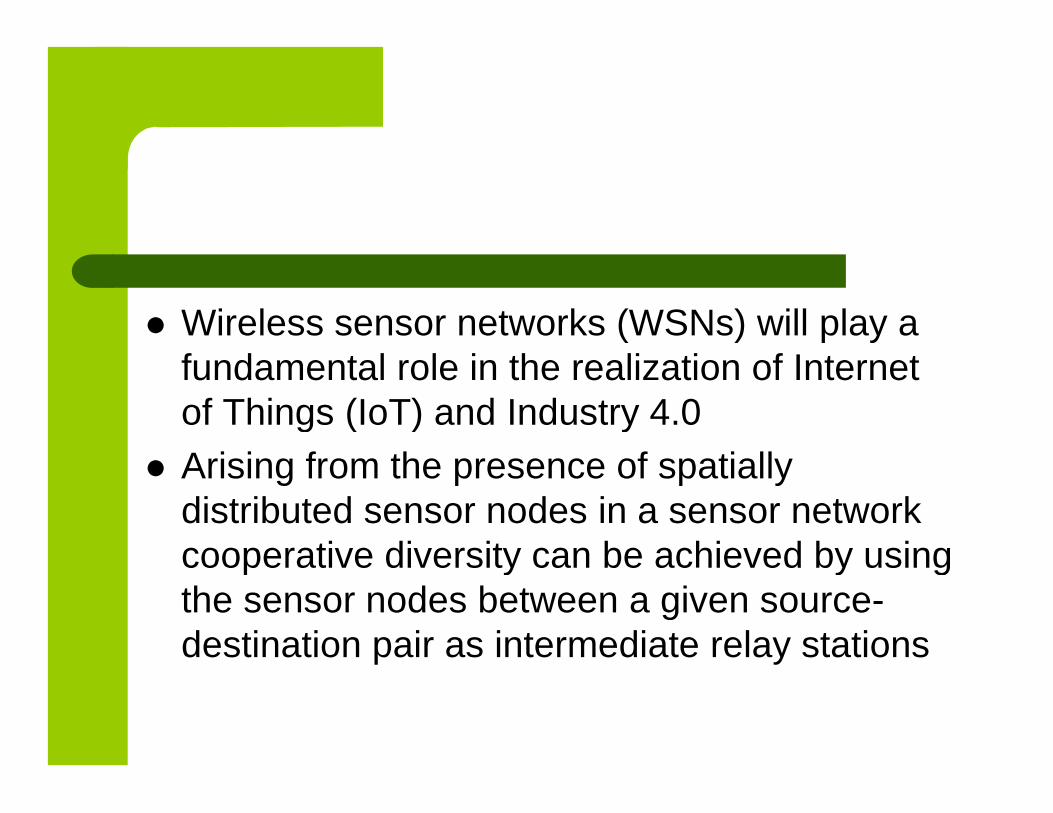
Wireless sensor networks (WSNs) will play afundamental role in the realization of Internetof Things (IoT) and Industry 4.0

Arising from the presence of spatiallydistributed sensor nodes in a sensor networkcooperative diversity can be achieved by usingthe sensor nodes between a given source-destination pair as intermediate relay stations

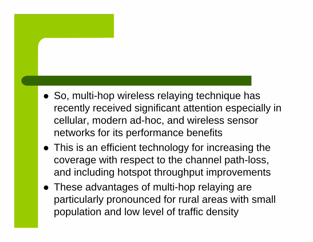
So, multi-hop wireless relaying technique hasrecently received significant attention especially incellular, modern ad-hoc, and wireless sensornetworks for its performance benefits

This is an efficient technology for increasing thecoverage with respect to the channel path-loss,and including hotspot throughput improvements

These advantages of multi-hop relaying areparticularly pronounced for rural areas with smallpopulation and low level of traffic density

The transmission characteristics of multi-hoprelaying systems have been widelyinvestigated

Significant attention is dedicated tocascaded fading channels which appear inwireless multi-hop transmission

Some references:

Rau´l Cha´vez-Santiago, Michał Szydełko, Adrian Kliks, Fotis Foukalas,Yoram Haddad, Keith E. Nolan, Mark Y. Kelly, Moshe T. Masonta,Ilangko Balasingham, “5G: The Convergence of WirelessCommunications”, Wireless Pers. Commun. 2015, 83:1617–1642, DOI10.1007/s11277-015-2467-2

Afif Osseiran, Volker Braun, Taoka Hidekazu, Patrick Marsch, Hans D.Schotten, Hugo Tullberg, Mikko Uusitalo, Malte Schellmann

“The Foundation of the Mobile and Wireless Communications Systemfor 2020 and Beyond: Challenges, Enablers and Technology Solutions”,IEEE 77th Vehicular Technology Conference (VTC Spring), 2-5 June2013, Dresden, Germany, DOI: 10.1109/VTCSpring.2013.6692781

The received signals are created as the productsof a large number of rays reflected via Nstatistically independent scatters

Therefore, the statistical analysis of products oftwo or more random variables (RVs) isintensified because of their applicability inperformance analysis of wireless relaycommunication systems with more hops(sections)

The wireless relay system output signal is aproduct of signal envelopes from eachsystem sections

Because of that, the cascade fading modelsare developed by the product of independentbut not necessarily identically distributedrandom variables

Many researchers are currently working inthis area and new cascade fading modelshave been suggested recently in theliterature

Due to this fact, the performance of productsof a higher number of random variables hasbecome an important topic over the pastdecade

The products of RVs are applied not only inwireless channel modeling, multi-hop relaysystems, multiple input multiple output(MIMO) keyhole systems, cascadedchannels with fading, but also in other naturalsciences, such as biology and physics(especially quantum physics), and also insocial sciences, econometrics, ...

In order to fill the gap areas in the literaturetied to cascaded models, an analysis hasbeen done here

This effort will surely help the researchersworking in this area, to be able to identify themost appropriate fading channel model for anefficient wireless relay communication systemdesign

In this tutorial, mostly a wireless multi-hop relaycommunication system operating in a multipathfading environment will be analyzed

The processes of derivation the system performanceof the first-order (probability density function (PDF),cumulative distribution function (CDF), outageprobability (OP), moments, amount of fading (AoF))and the second-order (level crossing rate (LCR) andaverage fade duration (AFD)) will be presented for

different fading distributions

The impact of the specific parameters willbe analyzed

Based on this analysis, it is possible toestimate the behavior of real systems inthe presence of fading

About fading

In wireless communications, fading isdeviation of the attenuation affecting a signalover propagation media

The fading may vary with time, geographicalposition or frequency, and it is modeled as arandom process

In wireless systems, fading may either bedue to multipath propagation, calledmultipath fading, or due to shadowing fromobstacles affecting the wave propagation

Multipath fading

Short-term fading (multipath fading) ispropagation phenomena caused byatmospheric, ionospheric reflection andrefraction, and reflection from water bodiesand terrestrial objects

Multipath fading degrades the systemperformance and limits the system capacity

Received signal experiences fading resultingin signal envelope variation

Shadowing

Shadowing is the result of the topographicalelements and other structures in thetransmission path such as trees, tallbuildings...

A log-normal or gamma distribution modelthe average power to account for shadowing

There are more distributions that can be used todescribe signal envelope variation in fadingchannels, which are dependent on propagationenvironment and communication scenario

They depend on existence of line of sightcomponent, nonlinearity of propagationenvironment, the number of clusters inpropagation channel, inequality of quadraturecomponents power and signal envelope powervariation

Various statistical models explain the natureof fading and several distributions describethe envelope of the received signal:Rayleigh, Rician, Nakagami-m, Hoyt orNakagami-q, Weibull, -µ, -κ-µ, κ-µ, -μ, …which was originally derived for reliabilitystudy purposes

A multipath fading channel is a communicationchannel containing multipath fading

The communication wireless relay mobile radiosystems will be consider in this lecture

A radio transmission system in whichintermediate radio stations or radio repeatersreceive and retransmit radio signals is knownas relay system

Wireless relay system can have several(two or more) sections

The desired signal in sections is subjectedto some kind of multipath fading

Outage probability

We need to determined the first and thesecond order system performance

The outage probability is important the firstorder performance measure of wirelesscommunication system which is defined asprobability that receiver output signalenvelope falls below of the specifiedthreshold and can be calculated fromcumulative distribution function

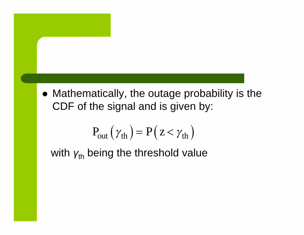
Mathematically, the outage probability is theCDF of the signal and is given by:

with γth being the threshold value

out th thP P z

There are two ways to define the outageprobability in wireless relay systems

For the first case, the outage probability isdefined as probability that the signal envelopein any sections falls below the specifiedthreshold

The outage probability for this case can becalculated as Cumulative Distribution Function(CDF) of minimum of signal envelopes fromsections

For the second case, the outage probability isdefined as probability that output signalenvelope falls down the determined threshold

The outage probability for this case is equal tothe CDF of product of signal envelopes atsections

Level crossing rate

Also, useful closed form expression foraverage level crossing rate (LCR) arecalculated for some cases

The level crossing rate is the second ordersystem performance

Average fade duration

The resulting integrals are solved forexample by using the Laplace approximatingformula or some other method

Later, the expression for LCR can be usedfor calculating the average fade duration(AFD) of proposed relay system

Wireless Relay System with Two Sectionsin κ-µ Short-Term Fading Channel

Dragana Krstić, Mihajlo Stefanovic, Radmila Gerov

Faculty of Electronic Engineering,University of Niš, Serbia

Zoran Popovic

Technical College of vocational studies

Zvečan, Serbia

The κ-µ distribution describes signalenvelopes in channels with dominantcomponents

The κ-µ distribution is characterized by twoparameters

The parameter κ is Rician factor, which is defined as the ratio of dominant componentpower and scattering components power

The parameter µ is related to the number ofclusters in propagation channel

The κ-µ small scale fading is more severe forless values of parameter µ

Also, the κ-µ multipath fading is more severefor lesser value of dominant componentpower and higher values of scatteredcomponents power

The κ-µ distribution is general distribution

The κ-µ distribution reduces

-to Nakagami-m distribution for κ=0,

-to Rician distribution for µ=1, and

-to Rayleigh distribution for κ=0 and µ=1

When Rician factor goes to infinity,κ-µ multipath fading channelbecomes no fading channel

Also, when parameter µ goes toinfinity, there is no fading in thechannel

PROBABILITY DENSITY FUNCTION AND CUMULATIVE

DISTRIBUTION FUNCTION OF MINIMUM OF TWO Κ-µRANDOM VARIABLES

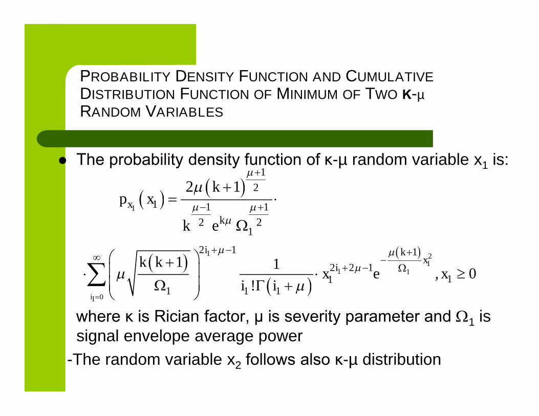
The probability density function of κ-µ random variable x1 is:

where κ is Rician factor, µ is severity parameter and 1 issignal envelope average power

-The random variable x2 follows also κ-µ distribution

1

1

2

1 1 1

2 21

2 1x

k

kp x

k e

1 21

1 1

01

2 1 1

2 2 111

1 1 1

1 1, 0

!i

i kx

ik kx e x

i i

Cumulative distribution function of x1 is:

where (n, x) is incomplete Gamma function of argument xand order n

Cumulative distribution function of x2 has the same shape

1

1

01

1 2 12

1 1 11 1 1

2 21

2 1 1 1

!i

i

x

k

k k kF x

i ik e

1

211 1 1

1

11, , 0

2 1

ik

i x xk

When the signal level at any section falls below thedefined threshold, the outage probability can becalculated from cumulative distribution function ofthe minimum of the signal envelopes at sections ofwireless communication system

Let analyze the minimum x of two random variablesx1 and x2, which is define as:

1 2min ,x x x

Probability density function of minimum x of tworandom variables is:

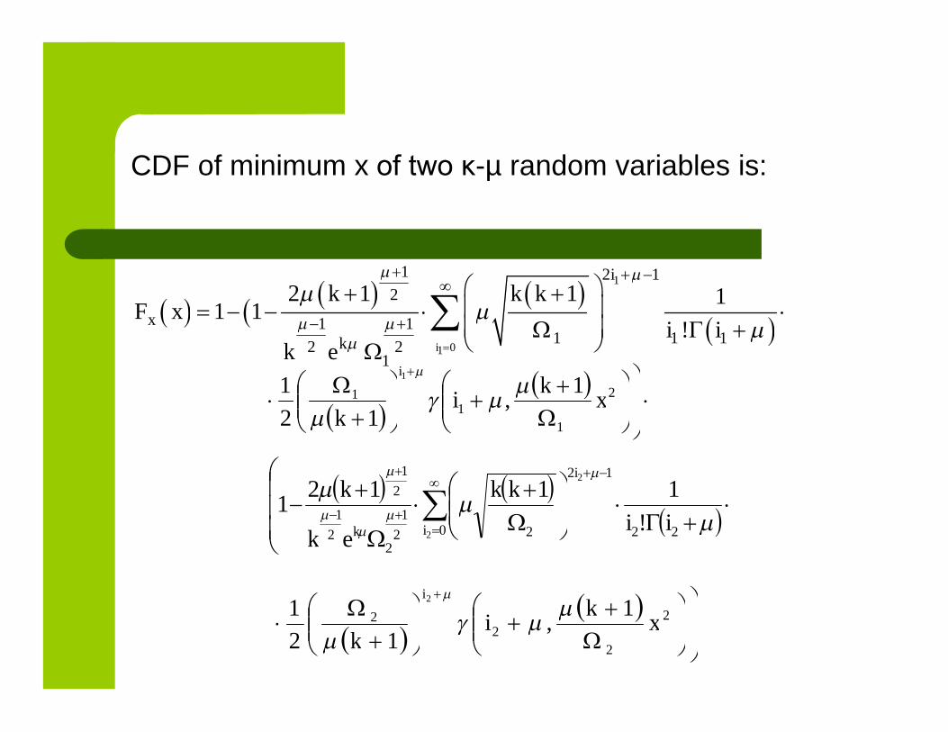
Cumulative distribution function of minimum x of tworandom variables is:

xFxpxFxpxp xxxxx 1221

( ) ( )( ) ( )( )1 21 1 1x x xF x F x F x= - - -

1

01

1 2 12

1 11 1 1

2 21

2 1 1 11 1

!i

i

k

x

k k k

i ik e

F x

2

1

11 1

,12

11

xk

ik

i

220

12

22

1

22

1

2

1

!

11121

2

2

ii

kk

ek

k

i

i

k

2

2

22 1

,12

12

xk

ik

i

CDF of minimum x of two κ-µ random variables is:

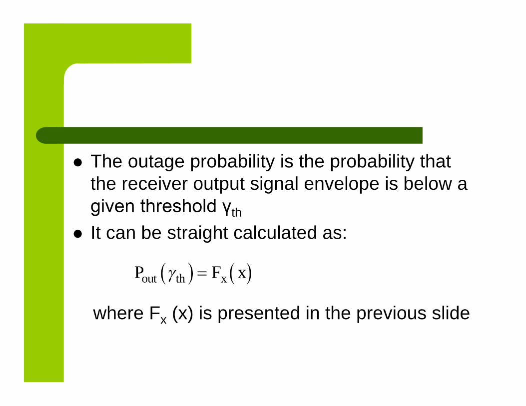
The outage probability is the probability thatthe receiver output signal envelope is below agiven threshold γth

It can be straight calculated as:

where Fx (x) is presented in the previous slide

out th xP F x

Here, CDFof minimum of two κ-µ randomvariables is the outage probability of wirelessrelay communication system with twosections over κ-µ multipath fading channel

Probability Density Function and CumulativeDistribution Function of Product of Two κ-µ RandomVariables

By the second definition, the outageprobability of wireless relay system can becalculated as probability that signal envelopeat the output of wireless relay communicationsystem falls below the predeterminedthreshold

For this case, the outage probability can becalculated as cumulative distribution functionof product of two κ-µ distributed signals.

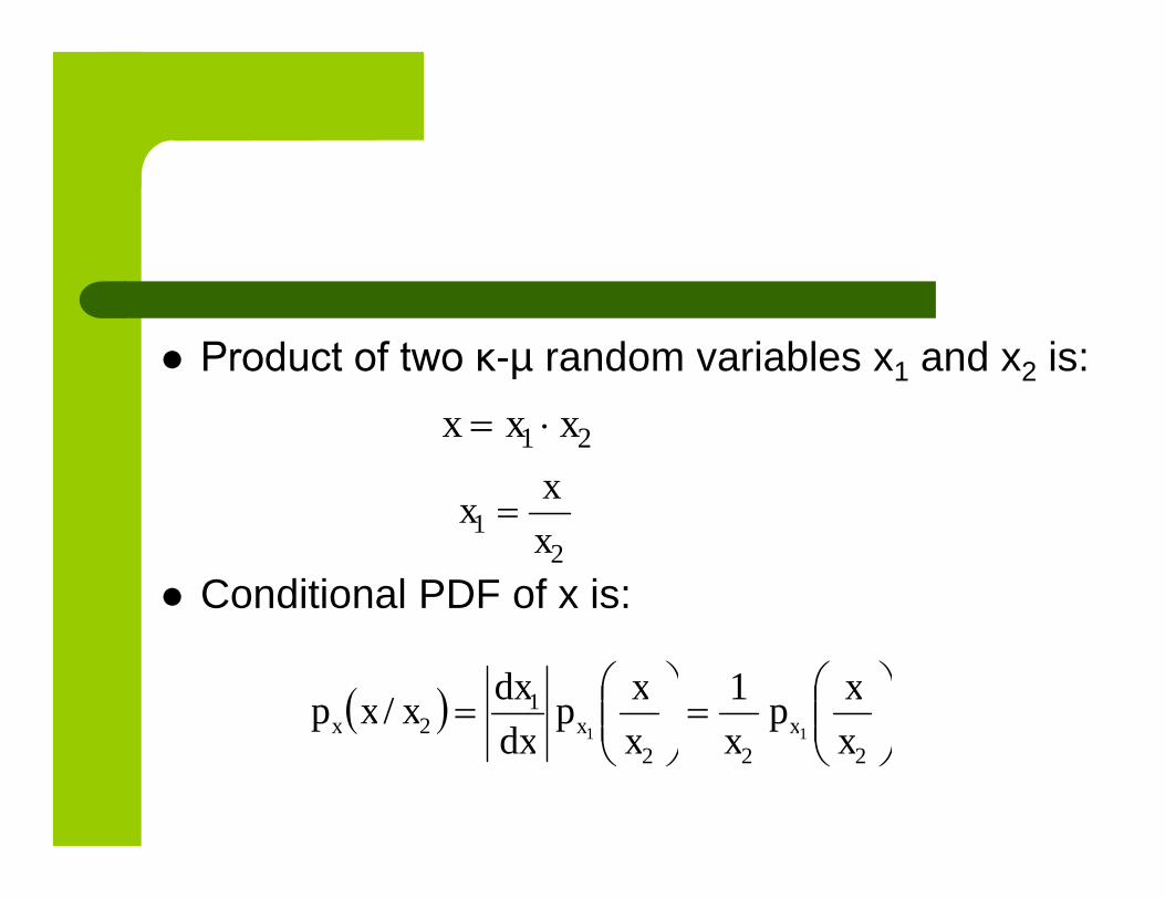
Product of two κ-µ random variables x1 and x2 is:

Conditional PDF of x is:

1 2x x x

12

xx

x

222

12 11

1/

x

xp

xx

xp

dx

dxxxp xxx

After integration, the expression for px(x) becomes:

1 22 2

2 20

1x x x

xp x dx p p x

x x

ii

kk

ek

k

i

i

k !

1112

10

12

12

1

12

1

2

1

2

1

220

12

22

1

22

1

2

1

!

1112

2

2

ii

kk

ek

k

i

i

k

2 1

1

2 1

22 222 2 1 2

2 21 1 2

12

i i

ii i

k xxx K

Cumulative distribution function of x is:

1

2

1 2 12

111100 22

1

2 1 1 1

!

ix

x x

ik

k k kF x dt p t

i ik e

220

12

22

1

22

1

2

1

!

1112

2

2

ii

kk

ek

k

i

i

k

122

2 1 2

12

2 2 1 12 12 2 2

2 1 20

11,

2 1

k ix

i i k xdx x e i

k x x

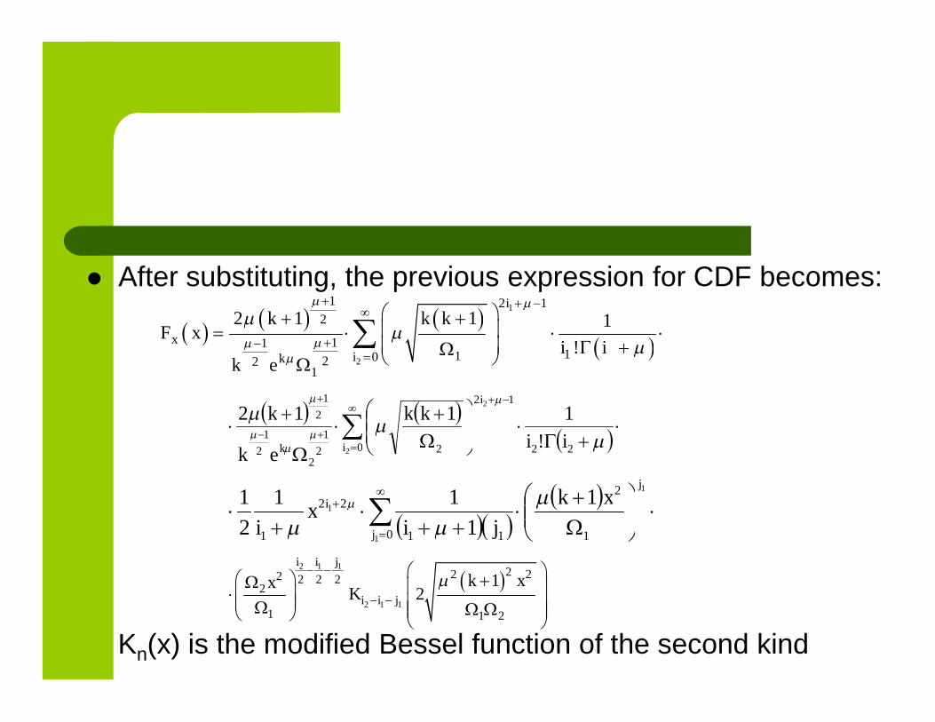
After substituting, the previous expression for CDF becomes:

Kn(x) is the modified Bessel function of the second kind

1

2

1 2 12

1111022

1

2 1 1 1

!

i

x

ik

k k kF x

i ik e

220

12

22

1

22

1

2

1

!

1112

2

2

ii

kk

ek

k

i

i

k

0 1

2

11

22

1 1

1

11

1

11

2

1

j

j

i xk

jix

i

2 1 1

2 1 1

22 22 2 2 22

1 1 2

12

i i j

i i j

k xxK

The cumulative distribution function ofminimum of two κ-µ random variables

NUMERICAL RESULTS

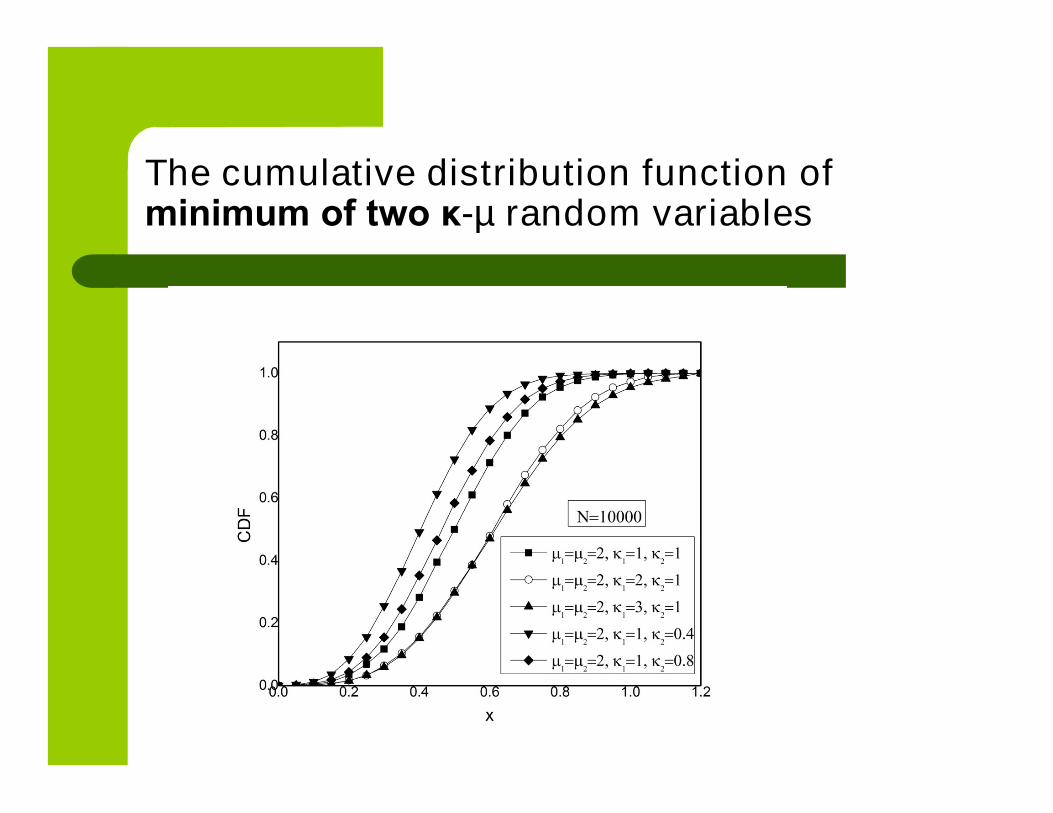
The cumulative distribution function of minimum oftwo κ-µ random variables versus signal envelope ispresented in previous Figure

The CDF is plotted for μ1=μ2=2 and variableparameters κ1 and κ2

It is visible that CDF increases with increasing of thesignal envelope

The cumulative distribution function decreases forlarger values of Rician factor κ1

Also, one can see from this figure that CDF is biggerfor higher values of Rician factor κ2

The cumulative distribution function of theproduct of two κ-µ random variables

The cumulative distribution function of product of two κ-µ random variables depending on the signal envelope ispresented in new Figure

The parameters μ1 and μ2 are equal to each other andhave a value of 2

It is possible to see from this Figure that CDF becomesbigger with increasing of the signal envelope

It shows that CDF is less for higher values of Ricianfactors κ1 and κ2

The system performance is better for smaller valuesof the outage probability, i.e., cumulative distributionfunction

This can be achieved by increasing the Riceanfactors κ1 and κ2

Since Rician factor is the ratio of dominantcomponent power and scattering componentspower, it is evident that bigger dominant componentpowers and smaller scattering components givebetter system performance

Conclusion 1

In this article, the communication relay radiosystem with two sections exposed to κ-µmultipath fading is analyzed

The outage probability is calculated in theclosed forms for the minimum and product oftwo random variables

The obtained formulas for the outage probability forrelay (κ-µ)*(κ-µ) channels could be used forcalculation the outage probability of other relaychannels

For κ1=0 and κ2=0, (κ-µ)*(κ-µ) relay channel reducesto Nakagami- Nakagami relay channel;

for µ1=1 and µ2=1, (κ-µ)*(κ-µ) channel becomesRician*Rician channel

Because of that, this article has general importance

Results of this analysis can be used bydesigners of relay systems in the case ofpresence of fading with κ-µ distribution

The designers of these systems can chooseoptimal parameters for given value of theoutage probability

Because of the generality of the results, thepresence of other types of fading can also becovered with this investigation

Wireless Relay System with TwoSections in the Presence of κ-µ and η-µ

Multipath Fading

Dragana Krstić, Vladeta Milenkovic,

Mihajlo Stefanović, Muneer Masadeh BaniYassein, Shadi Aljawarneh, Zoran Popovic

Probability Density Functions of κ-µRandom Variable and η-µ Random Variable

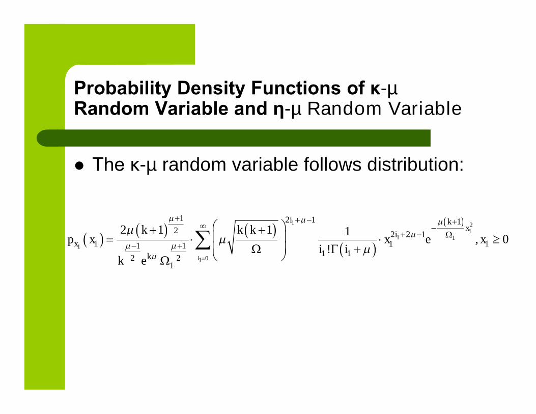
The κ-µ random variable follows distribution:

1 21

1 1

1

01

1 2 1 12 2 2 1

1 111 11 1

2 21

2 1 1 1, 0

!i

i kx

ix

k

k k kp x x e x

i ik e

The η-µ random variable follows distribution:

( )( )

2

22

221/222

2 1/2 21/22

1/22

4 2µhµµ µ x

x µµµ

µ h x µhp x e I x

µ H

p W+ -

-+-

æ ö÷ç ÷= =ç ÷ç ÷çè ø×

WG W

( ) ( )

22

2

2

22

22 1/21/24 4 1

221/21/20 2 22 2

4

!,

10

µhi µµ µ xi µ

µµi

µ h µhx e x

i i µµ H

p+ -+ -¥

+ - W+-

=

æ ö÷ç ÷= × × ³ç ÷ç ÷çW G +è øG Wå

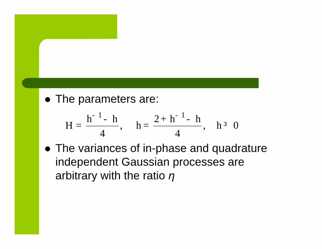
The parameters are:

The variances of in-phase and quadratureindependent Gaussian processes arearbitrary with the ratio η

1 12, , 0

4 4H h

h h h hh

- -- + -= = ³

Cumulative Distribution Functions of κ-µRandom Variable and η-µ Random Variable

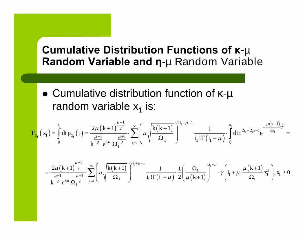
Cumulative distribution function of κ-µrandom variable x1 is:

1 21

1 1

1

0

1

1

1

1

1 2 1 12 2 2 1

1 11 1 1 02 2

10

2 1 1 1

!i

i kxt

x

k

x

ix

k k kt dt t e

i iF x dt p

k e

1 1

01

1 2 12

211 1 11 1

1 1 1 12 2

1

2 1 1 11 1, , 0

! 2 1i

i i

k

k k k ki x x

i i kk e

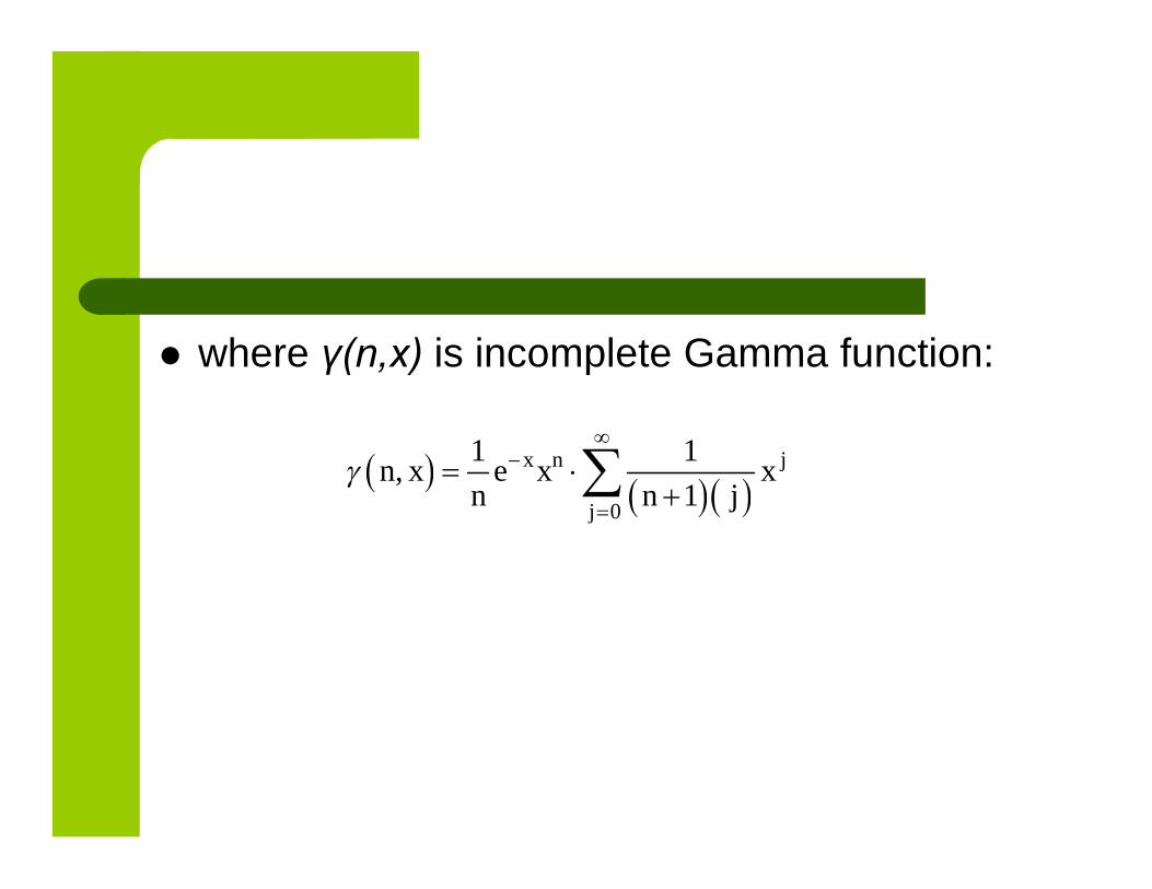
where γ(n,x) is incomplete Gamma function:

0

1 1,

1x n j

j

n x e x xn n j

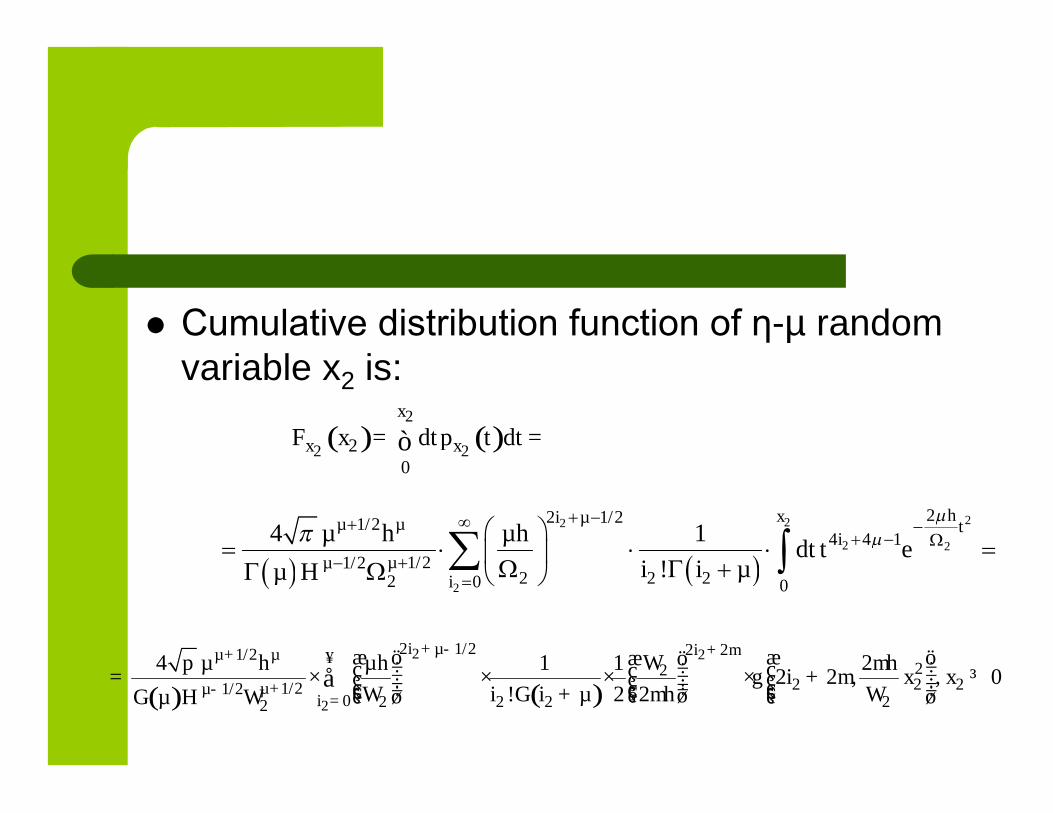
Cumulative distribution function of η-µ randomvariable x2 is:

( ) ( )2

22 20

x

x xF x dtp dtt= =ò

2 22

2 2

2

2 1/21/2

1/21/222

2

4

0

4 1

2 2 0

4 1

!

i µµ x

i

htµ

i

µµ

µ h µh

i i µdt t

µ He

( ) ( )

2

2

22 222

2 1/21/2

1/21/20 22

2 2 22 2 2

1 22 2 , , 0

2 2

4 1

!

i µµ µ

µi

i

µ

µ h µh

i i µ

hi x x

µ H h

mm

g mm

p+ -+ ¥

+-

+

=

æ ö÷ç ÷= × × ×ç ÷ç ÷çW G

æ öæ öW ÷÷ çç ÷÷ × + ³çç ÷÷ çç ÷ç ÷ç Wè è ø+è øG W øå

Minimum of κ-µ Random Variable and η-µRandom Variable

Minimum of random variables x1 and x2 is:

Cumulative distribution function of x is:

1 2min ,x x x

( ) ( )( ) ( )( )1 21 1 1x x xF x F x F x= - - -

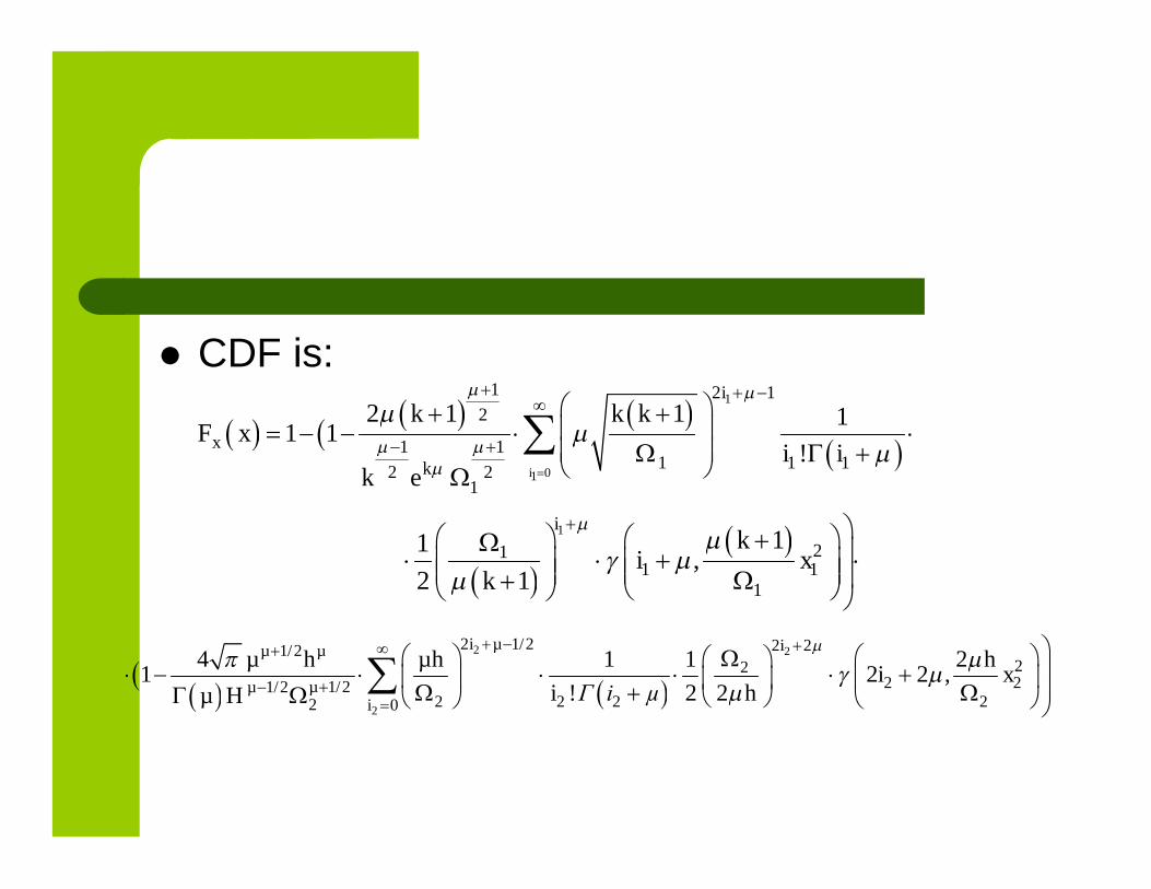
CDF is:

1

01

1 2 12

1 11 1 1

2 21

2 1 1 11 1

!i

i

k

x

k k k

i ik e

F x

22

2

2 1/21/2

1/21/2

2 222

22

22 20

22

4 11

!

1 22 2 ,

2 2

i µµ µ

µµi

iµ h µh

i Г i µµ H

hi x

h

1

211 1

1

11,

2 1

ik

i xk

Since the outage probability is actually theprobability that signal envelope becomessmaller than the determined threshold, theoutage probability of relay system can becalculated from cumulative distributionfunction of minimum of κ-µ random variableand η-µ random variable:

where x0 is the determined threshold

( )0 0xP F x=

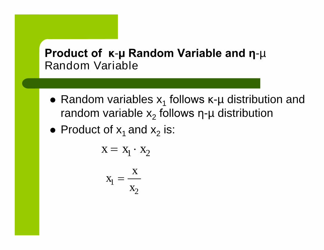
Product of κ-µ Random Variable and η-µRandom Variable

Random variables x1 follows κ-µ distribution andrandom variable x2 follows η-µ distribution

Product of x1 and x2 is:

1 2x x x

12

xx

x

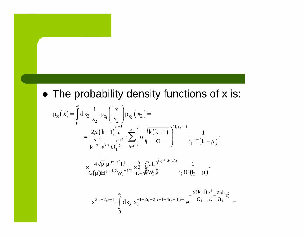
The probability density functions of x is:

1 22 2

2 20

1x x x

xp x dx p p x

x x

1

01

1 2 12

1 11 1

2 21

2 1 1 1

!i

i

k

k k k

i ik e

( ) ( )

2

2

2 1/21/2

1/21/220 2 22

4 1

!

i µµ µ

µµi

µ h µh

i i µµ H

p+ -+ ¥

+-=

æ ö÷ç ÷× × ×ç ÷ç ÷çW G +è øG Wå

22

21

2

211 2 2

2

1 2 2 1 4

1

4 12

22

2 1

0

µhx

i i

k x

i xµxx d ex

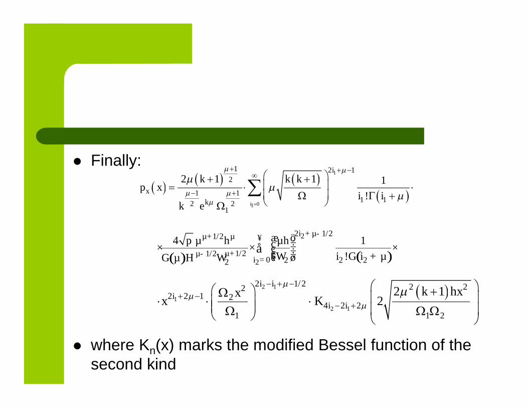
Finally:

where Kn(x) marks the modified Bessel function of thesecond kind

1

01

1 2 12

1 11 1

2 21

2 1 1 1

!i

i

x

k

k k kp x

i ik e

( ) ( )

2

2

2 1/21/2

1/21/220 2 22

4 1

!

i µµ µ

µµi

µ h µh

i i µµ H

p+ -+ ¥

+-=

æ ö÷ç ÷× × ×ç ÷ç ÷çW G +è øG Wå

2 1

1

2 1

2 1/2 2 222 2 1 2

4 2 21 1 2

2 12

i i

ii i

k hxxx K

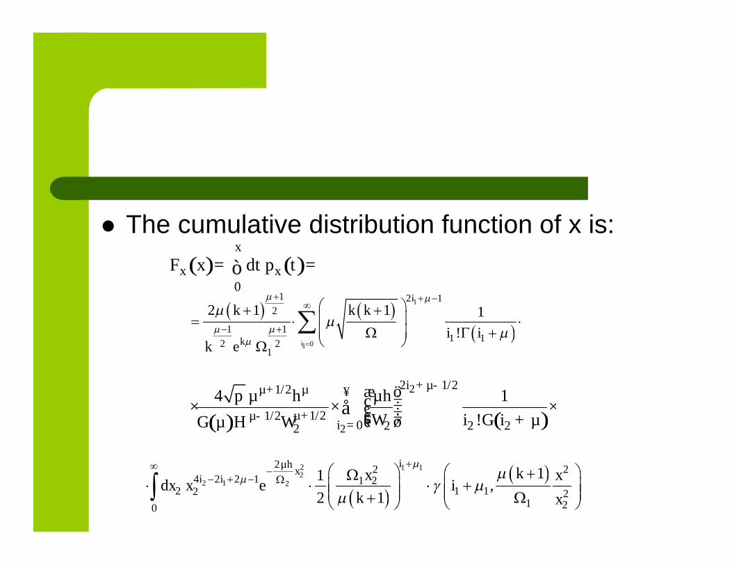
The cumulative distribution function of x is:

( ) ( )0

x

x xF x dt p t= =ò

1 1

2

22

21

22

12

4 2 2 1 21 1 2

1 20

2 2

11,

2 1

h

i

µ

ix

i

dxkx x

ik

xx

e

1

01

1 2 12

1 11 1

2 21

2 1 1 1

!i

i

k

k k k

i ik e

( ) ( )

2

2

2 1/21/2

1/21/220 2 22

4 1

!

i µµ µ

µµi

µ h µh

i i µµ H

p+ -+ ¥

+-=

æ ö÷ç ÷× × ×ç ÷ç ÷çW G +è øG Wå

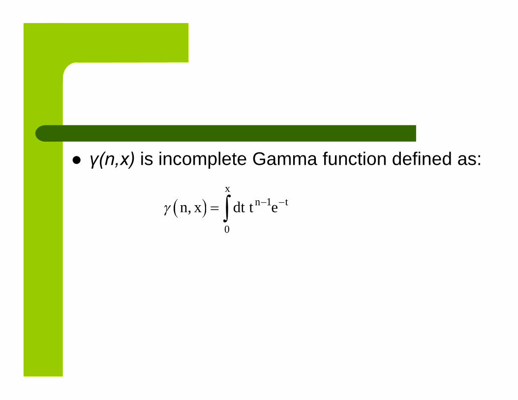
γ(n,x) is incomplete Gamma function defined as:

1

0

,

x

n tn x dt t e

Probability density function of minimum ofκ-µ random variable and η-µ random variablefor κ=1, µ=2 and η=1/4

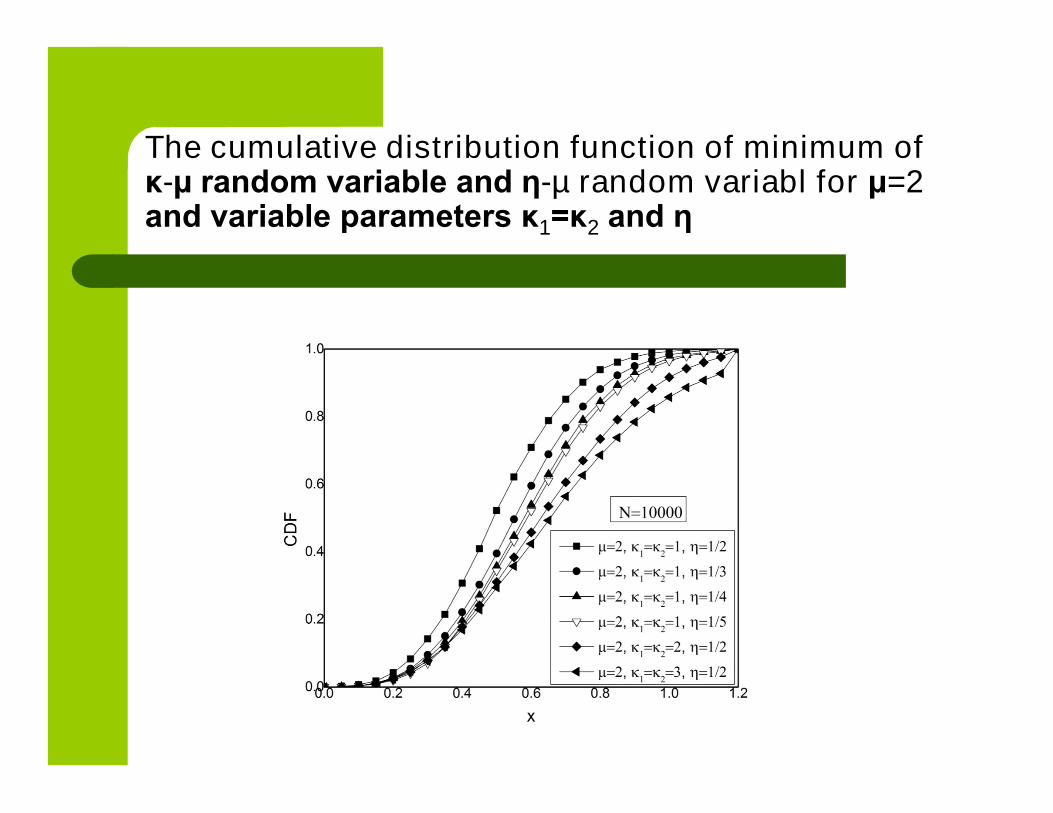
The cumulative distribution function of minimum ofκ-µ random variable and η-µ random variabl for μ=2and variable parameters κ1=κ2 and η

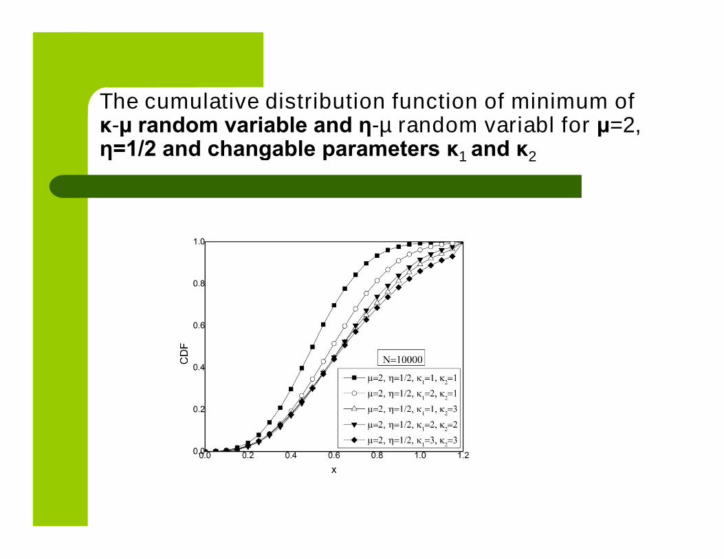
The cumulative distribution function of minimum ofκ-µ random variable and η-µ random variabl for μ=2,η=1/2 and changable parameters κ1 and κ2

The cumulative distribution function issmaller for lesser values of Rician factor κ

Also, one can see that CDF is bigger forbigger values of fading parameter η

It can be observed from Fig. 3 that CDFdecreases for larger values of Rician factorsκ1 and κ2

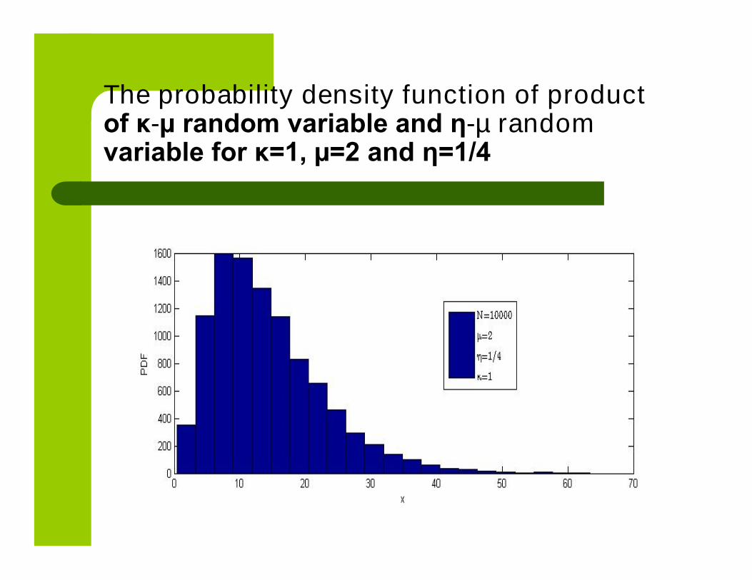
The probability density function of productof κ-µ random variable and η-µ randomvariable for κ=1, µ=2 and η=1/4

The cumulative distribution function of product of κ-µ random variable and η-µ random variable for μ=2and variable parameters η and κ1=κ2

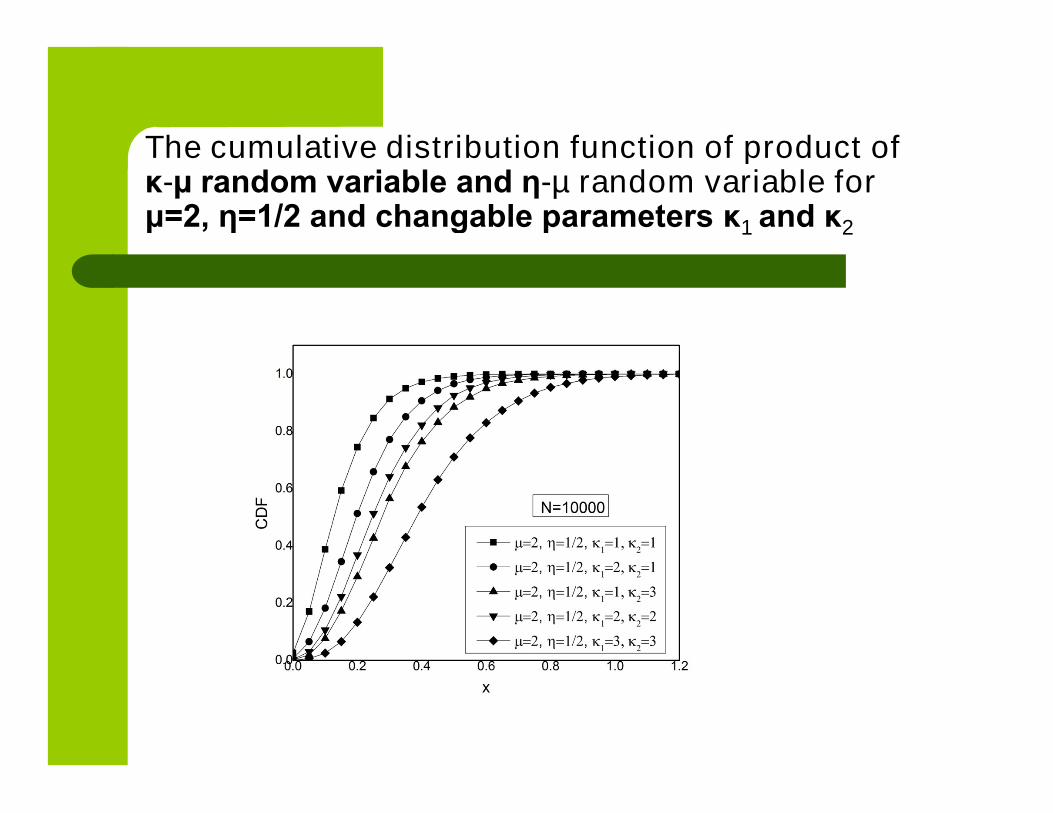
The cumulative distribution function of product ofκ-µ random variable and η-µ random variable forμ=2, η=1/2 and changable parameters κ1 and κ2

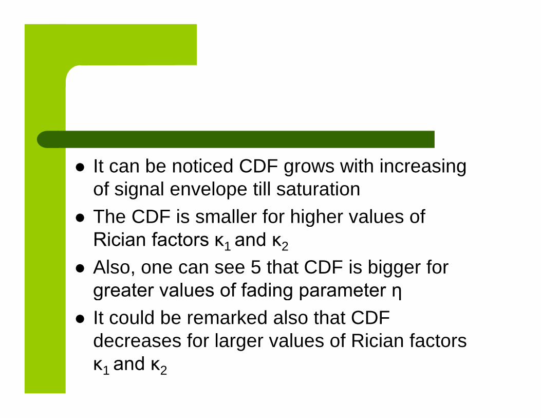
It can be noticed CDF grows with increasingof signal envelope till saturation

The CDF is smaller for higher values ofRician factors κ1 and κ2

Also, one can see 5 that CDF is bigger forgreater values of fading parameter η

It could be remarked also that CDFdecreases for larger values of Rician factorsκ1 and κ2

Conclusion 2

In this part, communication mobile relay radiosystem with two sections is analyzed when thefirst section is exposed to κ-µ multipath fadingand the second section is upset by η-µmultipath fading

In the channel of the first section the dominantcomponent is present

In the second section, the powers of in-phaseand quadrature components are different

The κ-µ random variable and η-µ randomvariable are general random variables, sothat obtained expressions for the outageprobability for relay channel (κ-µ), (η-µ) canbe used for evaluation the outage probabilityfor other relay channels

For κ=0 and η=1, (κ-µ), (η-µ) relay channelreduces to Nakagami, Nakagami relaychannel;

for µ1=1 and η=1, (κ-µ), (η-µ) distributionbecomes Rician, Nakagami-m relay channel;

for κ=0 and µ2=1, Nakagami-m, Nakagami-qdistribution may be obtained from (κ-µ), (η-µ)distribution

B. Talha, M. Patzold:

On the statistical properties of double Ricechannels,

Proceedings of 10th International Symposiumon Wireless Personal MultimediaCommunications, WPMC 2007, Jaipur, India,517-522

Some Performance of Three-hopWireless Relay Channels in the

Presence of Rician Fading

Dragana Krstic, Petar Nikolic, Sinisa Minic, ZoranPopovic

Outline

THE FIRST ORDER PERFORMANCE OF PRODUCT

OF THREE RICIAN RANDOM VARIABLES

– PDF of Product of Three Rician RVs

– CDF of Product of Three Rician RVs

– Outage probability of Product of ThreeRician RVs

THE SECOND ORDER PERFORMANCE OF THE

PRODUCT OF THREE RICIAN RANDOM

VARIABLES

– LCR of Product of Three Rician RVs

– AFD of Product of Three Rician RVs

A three-hop communication system, that weanalyze, is illustrated in the next figure

It consists of the source node, denoted by(S), sending the information signal to thedestination (D) with the help of twoconsecutive relays, namely R1 and R2

The AF relay nodes are assumed to beuntrusted and hence, they can overhear thetransmitted information signal while relaying

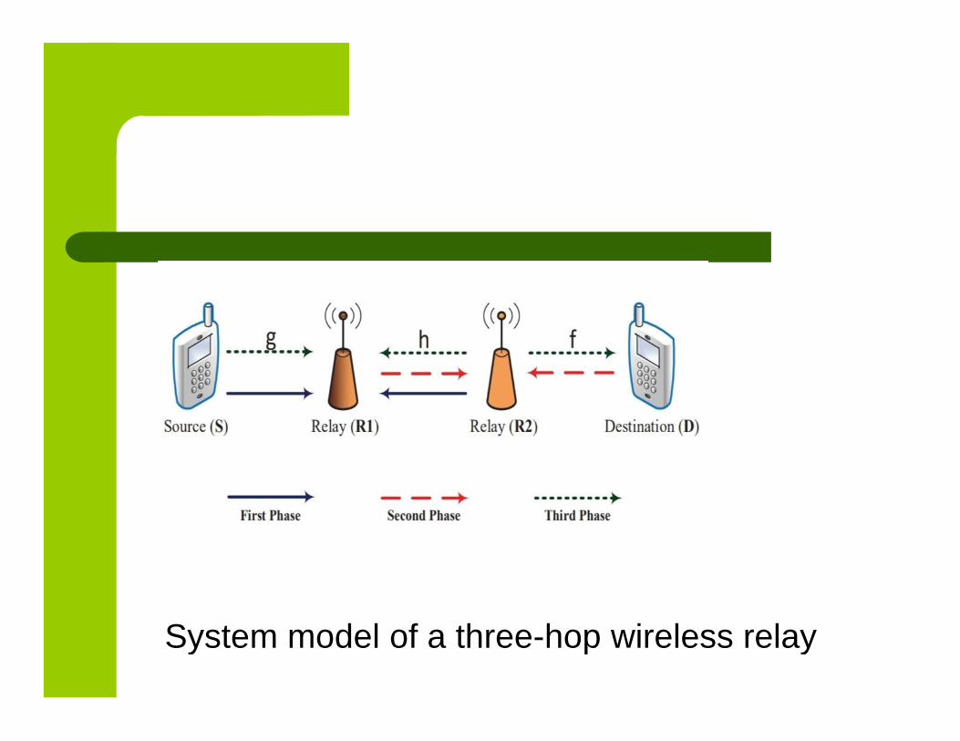
System model of a three-hop wireless relay

All nodes are equipped with a single antennaoperating in half-duplex mode

The consecutive relays are necessary helpers todeliver the information signal to the destination

This assumption is valid when the network nodesexperience a heavy shadowing, or when thedistance between terminals is large, or when thenodes suffer from limited power resources

For three-hop relay system we will obtain thesecond order characteristics

The knowledge of second-order statistics ofmultipath fading channels (level crossing rate(LCR) and average fade duration (AFD)) canhelp us better understand and mitigate theeffects of fading

For example, the AFD determines theaverage length of error bursts in fadingchannels

So, in fading channels with relatively largeAFD, long data blocks will be significantlyaffected by the channel fades than shortblocks

THE FIRST ORDER PERFORMANCE OF

PRODUCT OF THREE RICIAN RANDOM

VARIABLES

A) PDF of Product of Three Rician RVs

Rician fading is a stochastic model for radiopropagation where the signal arrives at thereceiver by several different paths when one ofthe paths, typically a line of sight signal or somestrong reflection signals, is much stronger thanthe others

In Rician fading, the amplitude gain ischaracterized by a Rician distribution

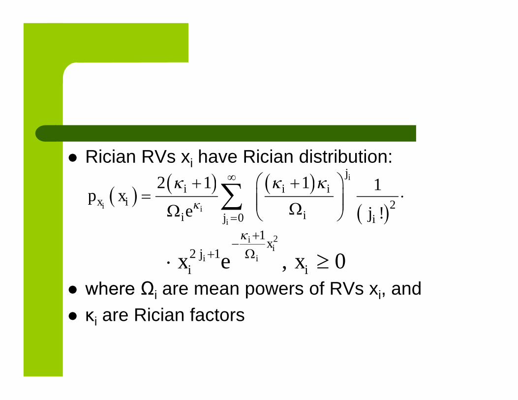
Rician RVs xi have Rician distribution:

where Ωi are mean powers of RVs xi, and

κi are Rician factors

2i 0

2 1 1 1

e !

i

i i

i

j

i i ix i

ij i

p xj

0,2

i

1

12

i

xj

i xexi

i

i

Rician factor is defined as a ratio of signalpower of dominant component and power ofscattered components

It can have values from [0, ]

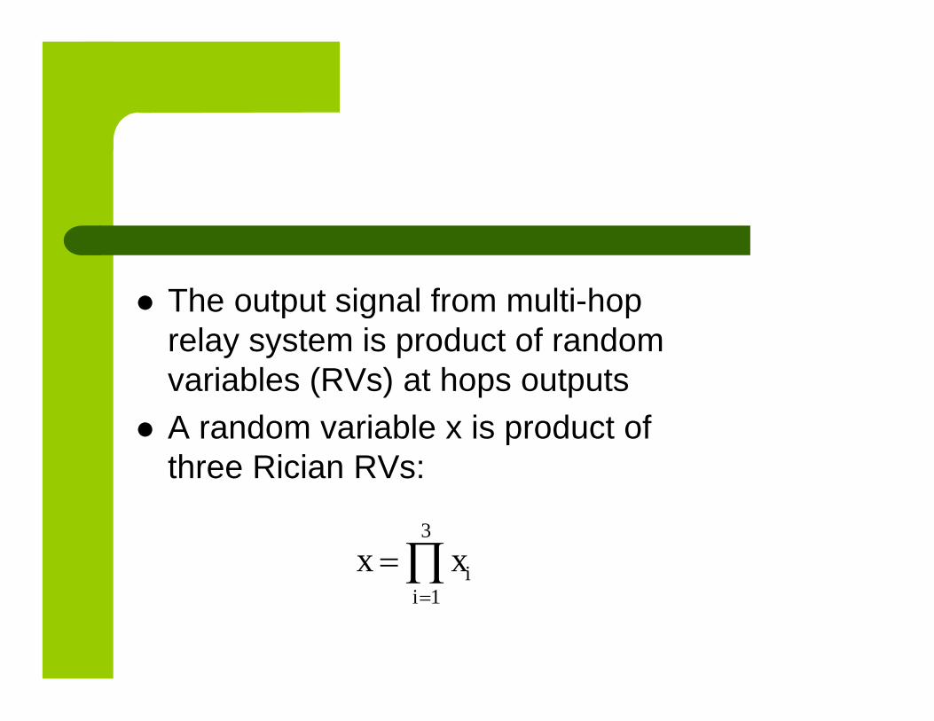
The output signal from multi-hoprelay system is product of randomvariables (RVs) at hops outputs

A random variable x is product ofthree Rician RVs:

3

1i

i

x x

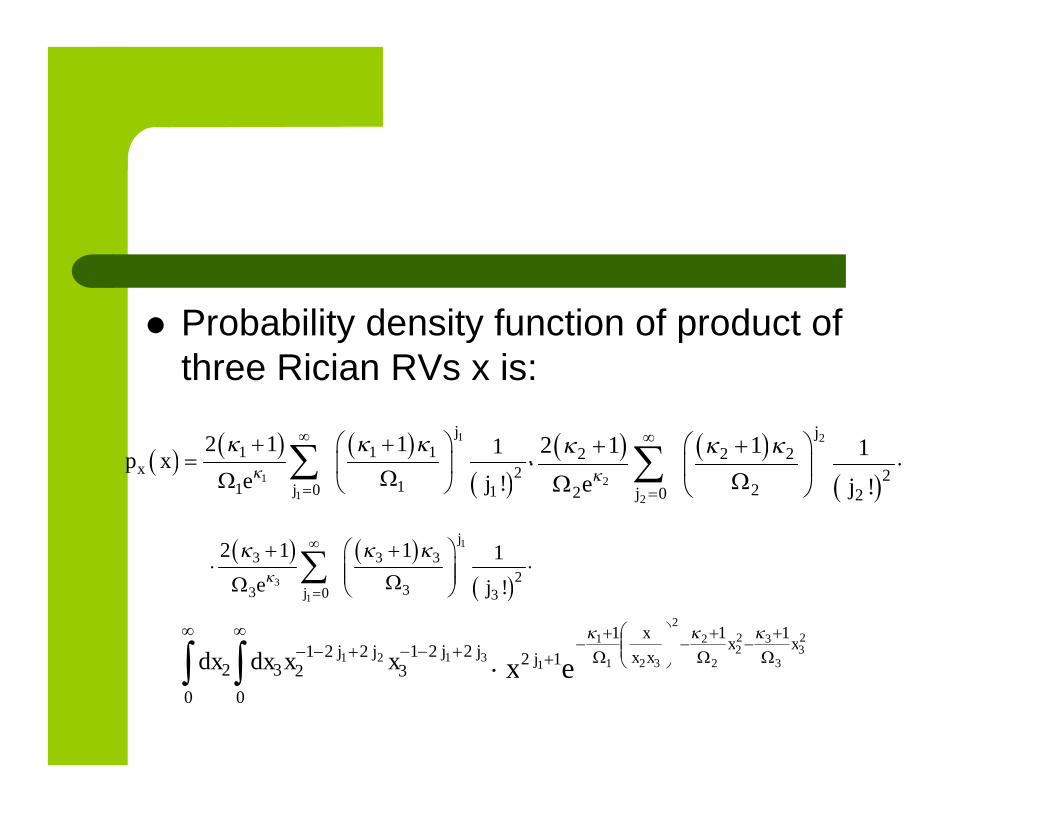
Probability density function of product ofthree Rician RVs x is:

1

1

1

1 1 1

211 0 1

2 1 1 1

e !

j

x

j

p xj

2

2

2

2 2 2

222 0 2

2 1 1 1

e !

j

j j

1

3

1

3 3 3

233 0 3

2 1 1 1

e !

j

j j

1 31 2 1 2 21 2 22 3 2 3

0 0

j jj jdx dx x x

23

3

322

2

2

2

321

1

1

111

12xx

xx

x

j ex

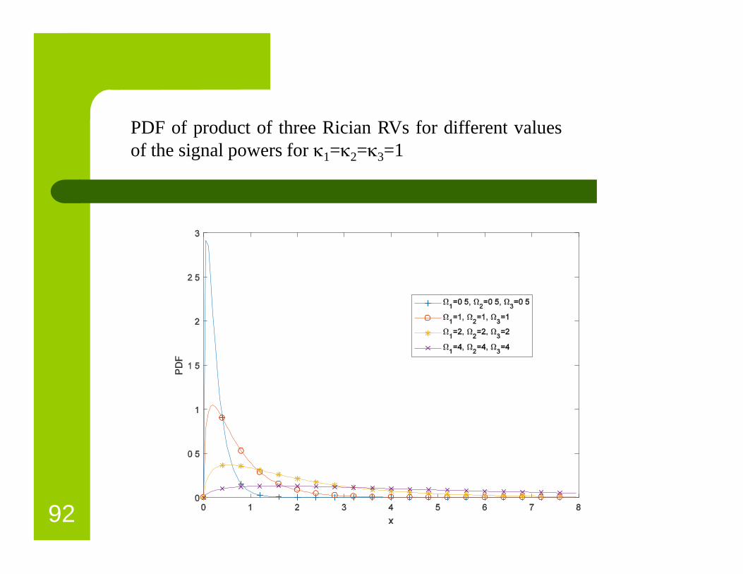
92

PDF of product of three Rician RVs for different valuesof the signal powers for 1=2=3=1

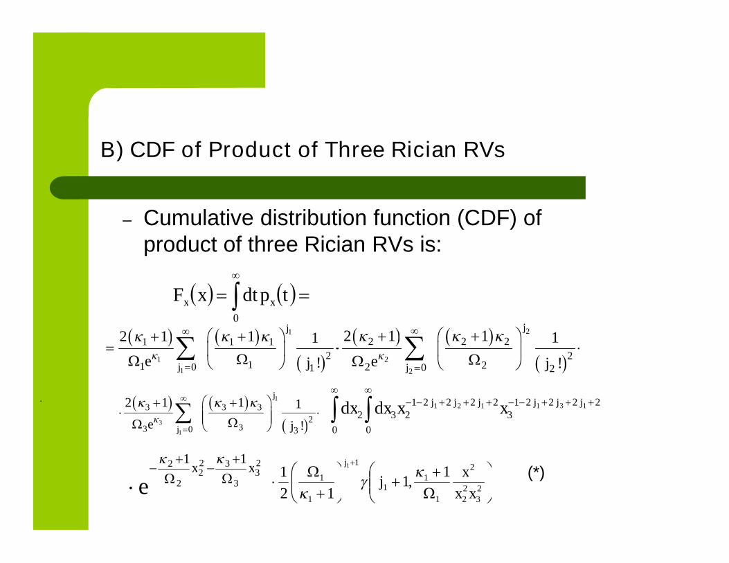
B) CDF of Product of Three Rician RVs

– Cumulative distribution function (CDF) ofproduct of three Rician RVs is:

tpdtxF xx

0

1

1

1

1 1 1

211 0 1

2 1 1 1

e !

j

j j

2

2

2

2 2 2

222 0 2

2 1 1 1

e !

j

j j

1

3

1

3 3 3

233 0 3

2 1 1 1

e !

j

j j

22221

322221

2

0

3

0

2131121

jjjjjj xxdxdx

23

3

322

2

2 11xx

e

23

22

2

1

11

1

1

1 1,1

12

11

xx

xj

j

.

(*)

Rayleigh fading is a model for stochastic fadingwhen there is no line of sight signal

Because of that it is considered as a specialcase of the more generalized concept of Ricianfading

Rayleigh fading is obtained for Rician factor κ=0

A case with κ →∞ present the scenario without fading

Since this reason, derived expressions for CDFof product of three Rician RVs can be used forevaluation a CDF of product of three RayleighRVs, also for CDF of product of two RayleighRVs and Rician RV, and CDF of product of twoRician RVs and Rayleigh RV

Obtained results can be used in performanceanalysis of wireless relay communication radiosystem with three sections in the presence ofmultipath fading

This means that derived CDFs are used for cases:

1) when Rician fading is present in all threesections ( , i=1,2,3), then

2) when Rayleigh fading is present in all threesections (κ1=κ2=κ3=0), the next

3) when Rayleigh fading is present in two sectionsand Rician in one (κ1=κ2=0, ) and

4) when Rayleigh fading is present in one andRician fading in two sections (κ1=0, , )

0i

3 0

3 0 2 0

The outage probability is an importantperformance measure of communication linksoperating over fading channels

Outage probability is defined as the probabilitythat information rate is less than the requiredthreshold information rate th

C) Outage probability of Product of Three Rician RVs

Pout is the probability that an outage will occurwithin a specified time period:

px(x) is the PDF of the signal and

th is the system protection ratio depending onthe type of modulation employed and thereceiver characteristics

Pout can be expressed as:

0

th

out xP p t dt

out x thP F

Plots of the outage probability, for differentvalues of parameters, are shown in Figs. 2 and 3

The choice of parameters is intended to illustratethe broad range of shapes that the curves of theresulting distribution can exhibit

It is evident that performance is improved withan increase in Rician factors I

Also, higher values of fading powers Ωi tend toreduce the outage probability and improvesystem performance, as it is expected

Fig. 2 Outage probability of product of three Rician RVs versus signalenvelope x for different values of Rician factor 1 and signal power Ω=1

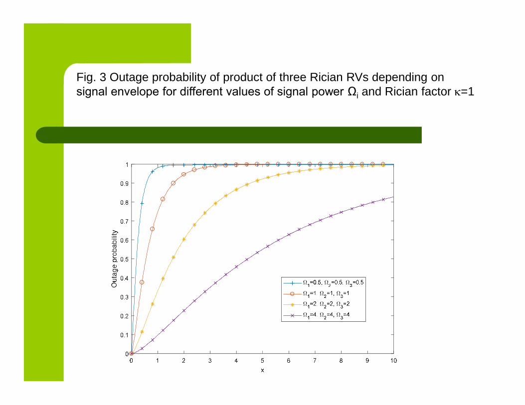
Fig. 3 Outage probability of product of three Rician RVs depending onsignal envelope for different values of signal power Ωi and Rician factor =1

Moments of Signals over Wireless RelayFading Environment with Line-of-Sight

Dragana Krstic, Petar Nikolic, Zoran Popovic, SinisaMinic, Mihajlo Stefanovic

INTRODUCTION

Moments present quantitative measure of the function’s shape

They are used in both, mechanics and statistics

When we deal with probability distribution, then:- zero-th moment is total probability,- the first one is mean of the signal (or expected value)- the second is the variance (or the average power of signal)- the third is skewness, and- the fourth moment is kurtosis

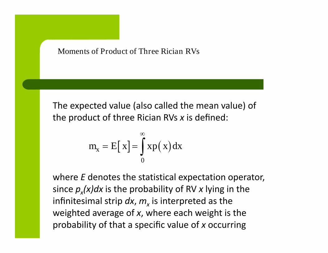
The expected value (also called the mean value) ofthe product of three Rician RVs x is defined:

where E denotes the statistical expectation operator,since px(x)dx is the probability of RV x lying in theinfinitesimal strip dx, mx is interpreted as theweighted average of x, where each weight is theprobability of that a specific value of x occurring

Moments of Product of Three Rician RVs

0

xm E x xp x dx

The expected value of a RV is an average of the valuesthat the RV takes in a large number of experiments andis called the first moment of a RV:

1

1

1

1 1 11 2

11 0 1

2 1 1 1

e !

j

j

m xj

2

2

2

2 2 2

222 0 2

2 1 1 1

e !

j

j j

1

3

1

3 3 3

233 0 3

2 1 1 1

e !

j

j j

23

3

3

31

22

2

2

21

1

2213

1

2212

0

3

0

2

xjj

xjj exexdxdx

2/323

221

2/3

1

1 1

1

2/312

1 jj

xxj

1

1

1

1 1 1

211 0 1

2 1 1 1

e !

j

j j

2

2

2

2 2 2

222 0 2

2 1 1 1

e !

j

j j

1

3

1

3 3 3

233 0 3

2 1 1 1

e !

j

j j

1 23/2 3/2

1 21 2

1 2

1 13 / 2 3 / 2

2 1 2 1

j j

j j

2/312

13

2/3

3

3

3

j

j

The first moment for the product of three RicianRVs is shown graphically in the next two figures

One can see that the first moment for productof three Rician RVs depending on Rician factor for a few values of signal power Ω=Ω1=Ω2=Ω3 isbigger for higher values of Ωi

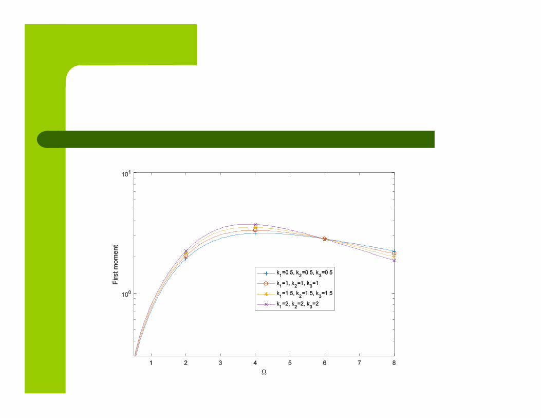
It is possible to notice from figure below anincreasing of the first moment with increasing ofΩ till maximal values

Then, m1 start to decline

For small Ω, m1 is higher for higher values ofRician factor

The second moment is known as the mean-squaredvalue of the RV, or variance or the signal's average power

The positive square root of the second moment(variance) is the standard deviation

In wireless communication we are speaking aboutsignal’s average power

The second moment m2 of the product of threeRician RVs is:

xpxxdxm 2

0

22

1

1

1

1 1 1

211 0 1

2 1 1 1

e !

j

j j

2

2

2

2 2 2

222 0 2

2 1 1 1

e !

j

j j

1

3

1

3 3 3

233 0 3

2 1 1 1

e !

j

j j

1 22 2

1 21 2

1 2

1 12 2

2 1 2 1

j j

j j

212

13

2

3

3

3

j

j

.

The influence of parameters of fadingdistribution to the second moment of product ofthree Rician RVs can be noticed from next figuresOne can see from these figures that the secondmoment, variance, enlarges with increasing ofpower ΩFor bigger Ω and Rician factor , m2 decreases

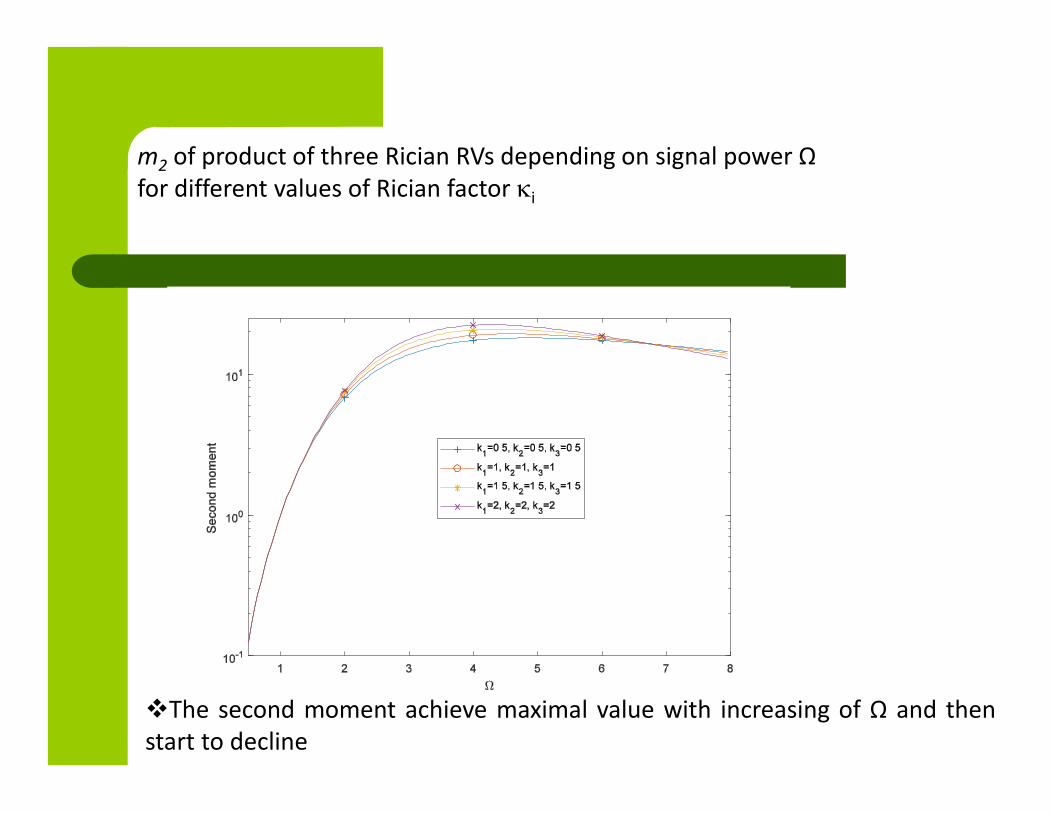
m2 of product of three Rician RVs depending on signal power Ω for different values of Rician factor i

The second moment achieve maximal value with increasing of Ω and thenstart to decline

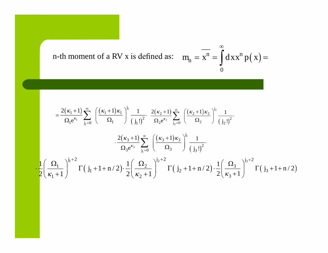
n-th moment of a RV x is defined as: 0

n nnm x dxx p x

1

1

1

1 1 1

211 0 1

2 1 1 1

e !

j

j j

2

2

2

2 2 2

222 0 2

2 1 1 1

e !

j

j j

1

3

1

3 3 3

233 0 3

2 1 1 1

e !

j

j j

1 22 2

1 21 2

1 2

1 11 / 2 1 / 2

2 1 2 1

j j

j n j n

3 2

33

3

11 / 2

2 1

j

j n

AoF of Product of Three Rician RVs

The amount of fading (AoF) is a measure of severity of fading for observedchannel

For defined distribution of power of a received signal, AoF is a ratio of thevariance of the received energy to the square of the mean of the receivedenergy

2

2 2/AoF Var x E x

- E· is statistical average value- Var· denoting the variance

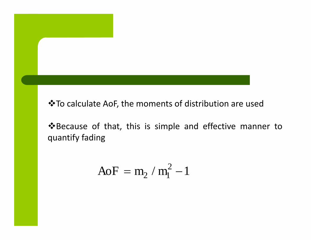
To calculate AoF, the moments of distribution are used

Because of that, this is simple and effective manner toquantify fading

22 1/ 1AoF m m

The range of values of AoF is given in interval [0, 2]

AoF=0 corresponds a situation of “no fading”

AoF=1 corresponds to a single Rayleigh fadingchannel

AoF= 2 refers to one-sided Gaussian distribution; thisis the severest fading

AoF of product of three Rician RVs versus Rician factor for different Ωi

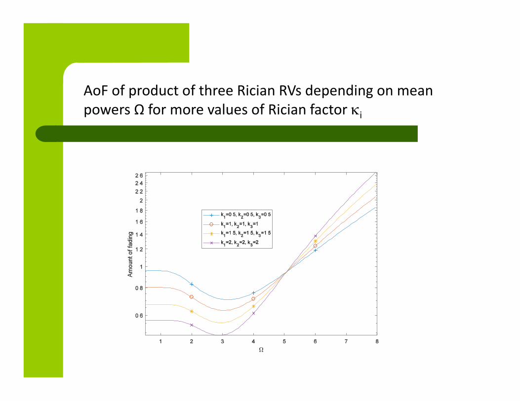
AoF of product of three Rician RVs depending on meanpowers Ω for more values of Rician factor i

It is visible that AoF increases with increasingof Ω for bigger values of Ω

For higher values of i and small Ω, AoF hassmaller values, but the situation is reversed forbigger Ω where AoF has higher values forhigher Rician factor

THE SECOND ORDER PERFORMANCE OF THE PRODUCT OF

THREE RICIAN RANDOM VARIABLES

Level crossing rate (LCR) and averagefade duration (AFD) of the signalenvelope are two important second-orderstatistics of wireless channel

They give useful information about thedynamic temporal behavior of multipathwireless fading channels

Level crossing rate is one of the mostimportant second-order performancemeasures of wireless communication system,which has already found application inmodelling and design of communicationsystem but also in the design of errorcorrecting codes, optimization of interleavesize and throughput analysis

A) LCR of Product of Three Rician RVs

The envelope LCR is defined as theexpected rate (in crossings per second) atwhich a fading signal envelope crosses thegiven level in the downward direction

The LCR of RV tells how often the envelopecrosses a certain threshold x

We should determine the jointprobability density function (JPDF)between x and , first, thenapply the Rice’s formula to finallycalculate the LCR

LCR is defined as:

x xxp xx

0

xxx d xx p xN x

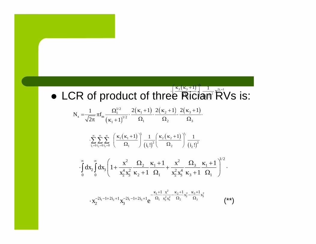
LCR of product of three Rician RVs is:

1/231 21

1/21 2 31

2 12 1 2 11

2 1x mN f

1 2

1 2 3

1 1 2 2

2 20 0 0 1 21 2

1 11 1

! !

i i

i i i i i

3

13 3 2 1

2

33

1 1

!

i

ixi

1/22 232 1 1

2 3 4 2 2 42 1 3 10 0 2 3 2 3

1 11

1 1

x xdx dx

x x x x

22 231 22 32 2

1 3 2 31 2 1 2 3

11 1

2 1 2 12 1 2 12 3

xx x

i i x xi ix x e

(**)

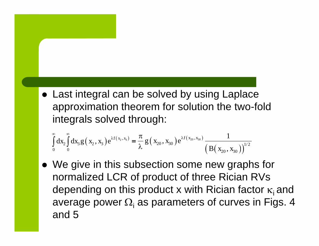
Last integral can be solved by using Laplaceapproximation theorem for solution the two-foldintegrals solved through:

We give in this subsection some new graphs fornormalized LCR of product of three Rician RVsdepending on this product x with Rician factor i andaverage power i as parameters of curves in Figs. 4and 5

2 3,

2 3 2 3

0 0

,f x x

dx dx g x x e

20 30,

120 30

20

/

3

2

0

,,

1xf xg x e

Bx

x x

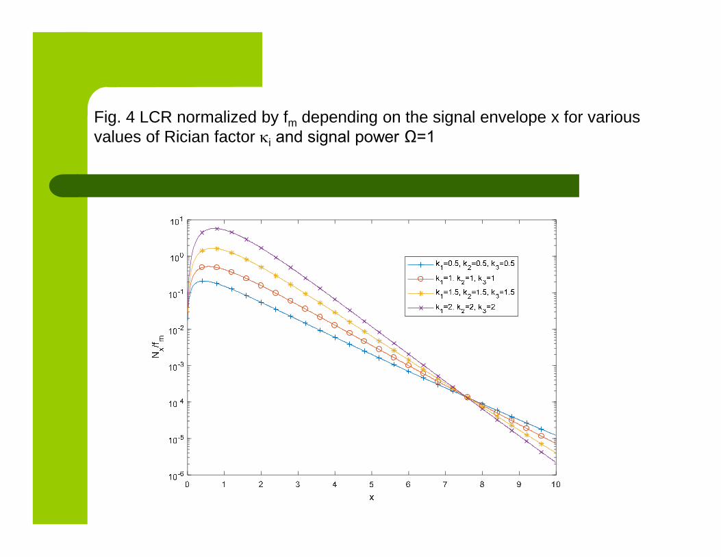
Fig. 4 LCR normalized by fm depending on the signal envelope x for variousvalues of Rician factor i and signal power Ω=1

Fig. 5 LCR normalized by fm versus signal envelope x forvarious values of signal powers Ωi

LCR grows as Rician signal power increases

The impact of signal envelope power on the LCRis higher for bigger values of Rician factor I

LCR increases with increasing of Ωi for all valuesof signal envelope

The impact of signal envelope on the LCR is largerfor higher values of the signal envelope when Ωi

changes

It is important bring to mind that system has betterperformance for lower values of the LCR

Average fade duration measures how long asignal’s envelope or power stays below a giventarget threshold derived from the LCR

According to that, AFD is:

The numerator is the cumulative distributionfunction of x from Eq. (*), and Nx (x) is LCRobtained by solving (**)

xN

dxxp

xN

XxPxT

x

X

x

x

x

0

B) AFD of Product of Three Rician RVs

The normalized AFD (Txfm) of product of threeRician RVs is plotted in Figs. 6 and 7 versussignal envelope x

One can see that for higher values of i andlower x, AFD has smaller values

Also, it is visible from Fig. 7 that AFD increasesfor all signal envelopes and lower Ωi

The impact of Ωi is bigger at higher envelopes

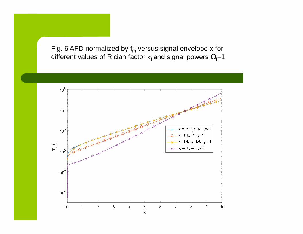
Fig. 6 AFD normalized by fm versus signal envelope x fordifferent values of Rician factor i and signal powers Ωi=1

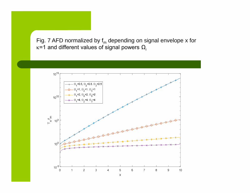
Fig. 7 AFD normalized by fm depending on signal envelope x for=1 and different values of signal powers Ωi

Conclusion 3

In this part, formulas for the PDF, CDF, Pout,LCR and AFD of the three-hop wireless relaysystem in the presence of Rician fading arederived

This system output signal is product of threeRician RVs

I. Ghareeb, D. Tashman,

“Statistical Analysis of Cascaded Rician FadingChannels”,

International Journal of Electronics Letters,ISSN: 2168-1724 (Print) 2168-1732 (Online),2018, doi:10.1080/21681724.2018.1545925

Exact-form expressions for the PDF and theCDF for product of n-Rician independent andnot necessarily identically distributed RVs areobtained in that paper

Moreover, expressions for the PDF and CDF ofthe instantaneous signal-to-noise ratio (SNR) inslow frequency nonselective independent andnot necessarily identically distributed cascadedRician fading channels are introduced andanalyzed

Exact-form expressions for the outageprobability and average channel capacity arealso derived

The average bit error probability (BEP)expression for phase-shift keying (PSK) signalsoperating in additive white Gaussian noise(AWGN) channel as well as in independent butnot necessarily identically distributed cascadedRician fading channels are derived

Outage Probability of Wireless RelayCommunication System with

Three Sections in the Presence ofNakagami-m Short Term Fading

Danijela Aleksić, Dragana Krstić,

Zoran Popović, Ivana Dinić, Mihajlo Stefanović

The wireless relay communication system with threesections operating over Nakagami-m multipathfading channel is the topic of this part

The outage probability of proposed relay system iscalculated again for two cases

In the first case, the outage probability is evaluatedwhen it is defined as probability that signal envelopefalls below the specified threshold at any sectionusing cumulative distribution function of minimum ofthree Nakagami-m random variables

In the second case, the outage probability iscalculated when it is defined as probability thatoutput signal envelope is lower thanpredetermined threshold by using the cumulativedistribution function of product of three Nakagami-m random variables

Numerical expressions for the outage probability ofrelay system are presented graphically and theinfluence of Nakagami-m parameter from eachsection on the outage probability is estimated

Nakagami-m distribution has some advantagesversus the other models, such as that this is ageneralized distribution which can modeldifferent fading environments

It has greater flexibility and accuracy inmatching some experimental data than theRayleigh, lognormal or Rice distributions

Rayleigh and one-sided Gaussian distributionare special cases of Nakagami-m model

So the Nakagami-m channel model is ofmore general applicability in practical fadingchannels

Nakagami-m statistical model describessignal envelope in non line of sight (LOS),linear multipath fading channel where signalpropagates with one, two or more clusters

Nakagami-m distribution has severityparameter m and signal envelope averagepower Ω

The parameter m is is greater than 0.5

When parameter m is equal to one, Nakagami-mdistribution reduces to Rayleigh distribution;

when parameter m tends to 0.5, Nakagami-mstatistical model turn into one sided Gaussianstatistical model and

when parameter m goes to infinity, Nakagami-mmultipath fading channel becomes no fadingchannel

Here, considered wireless relay system hasthree sections and Nakagami-m fading ispresent in channel’s sections

This channel can be denoted as Nakagami-Nakagami- Nakagami channel

It has three parameters which are denotedwith m1, m2 and m3

Also, Nakagami- Nakagami- Nakagami relaychannel is general channel and severalchannels can be derived from this channel

For m1=1, Nakagami- Nakagami- Nakagamichannel becomes Rayleigh- Nakagami-Nakagami channel;

for m1=1 and m2=1, Nakagami- Nakagami-Nakagami channel becomes Rayleigh -Rayleigh - Nakagami channel, and

for m1=1, m2=1 and m3=1, Nakagami-Nakagami- Nakagami channel becomesRayleigh- Rayleigh – Rayleigh channel

For m1=0.5, Nakagami- Nakagami-Nakagami channel becomes One sidedGaussian- Nakagami- Nakagami channel;

for m1=0.5 and m2=0.5, Nakagami-Nakagami- Nakagami channel becomes Onesided Gaussian- One sided Gaussian-Nakagami channel, and

for m1=1/2, m2=1/2 and m3=1/2, Nakagami-Nakagami- Nakagami channel becomes Onesided Gaussian- One sided Gaussian- Onesided Gaussian relay channel

Also, for m1 goes to infinity, Nakagami- Nakagami-Nakagami relay channel becomes no fading-Nakagami- Nakagami channel

for m1 goes to infinity and m2 goes to infinity,Nakagami- Nakagami- Nakagami relay channelbecomes no fading- no fading - Nakagami relaychannel, and

for m1 goes to infinity, m2 goes to infinity and m3 goesto infinity, Nakagami- Nakagami- Nakagami relaychannel becomes no fading- no fading - no fadingchannel

Statistics of Minimum of ThreeNakagami Random Variables

Random variables x1, x2 and x3 follow Nakagami-mdistribution:

2111

1 1

1

2 111 11

1 1

2, 0

mmx

mx

mp x x e x

m

2222

2 2

2

2 122 22

2 2

2, 0

mmx

mx

mp x x e x

m

2313

3 3

3

2 133 33

3 3

2, 0

mmx

mx

mp x x e x

m

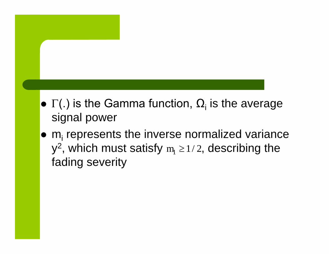
(.) is the Gamma function, Ωi is the averagesignal power

mi represents the inverse normalized variancey2, which must satisfy , describing thefading severity

1 1/ 2m

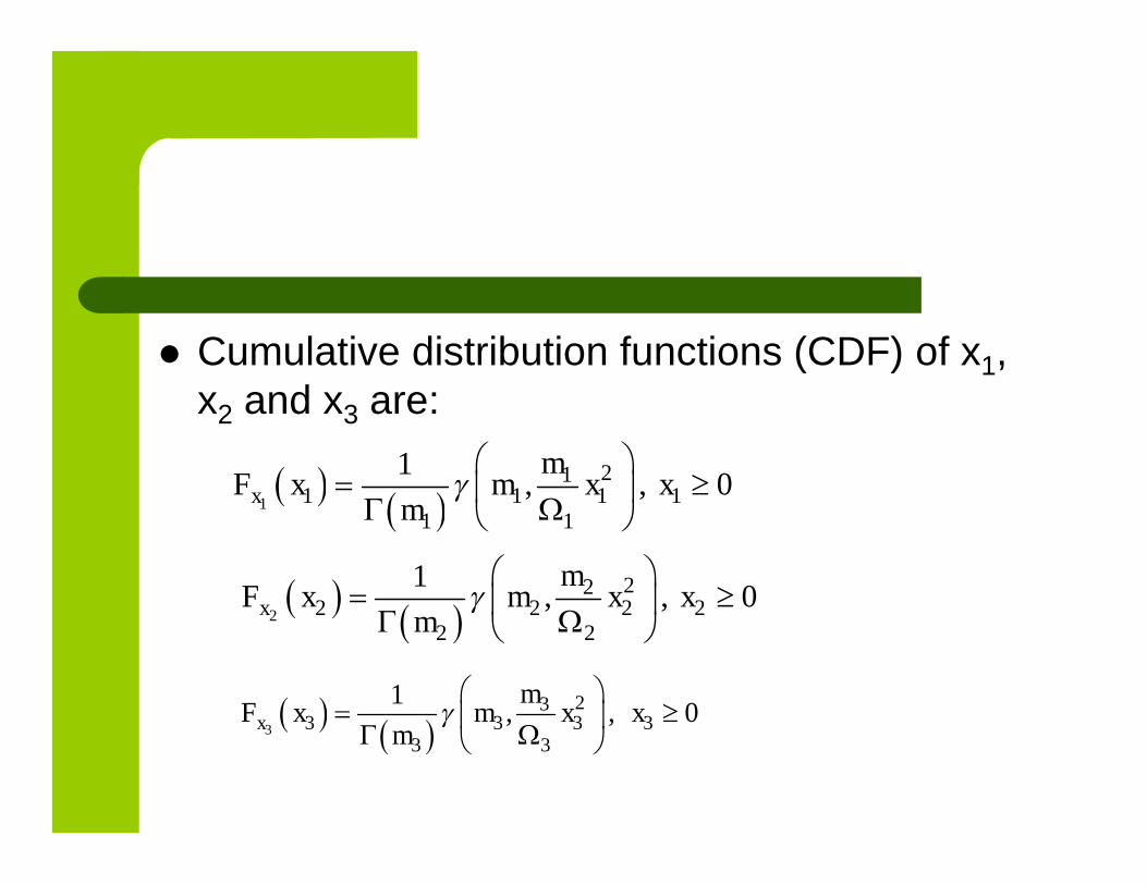
Cumulative distribution functions (CDF) of x1,x2 and x3 are:

1

211 1 1 1

1 1

1, , 0x

mF x m x x

m

2

222 2 2 2

2 2

1, , 0x

mF x m x x

m

3

233 3 3 3

3 3

1, , 0x

mF x m x x

m

Minimum of x1, x2 and x3 is:

1 2 3min( , , )x x x x

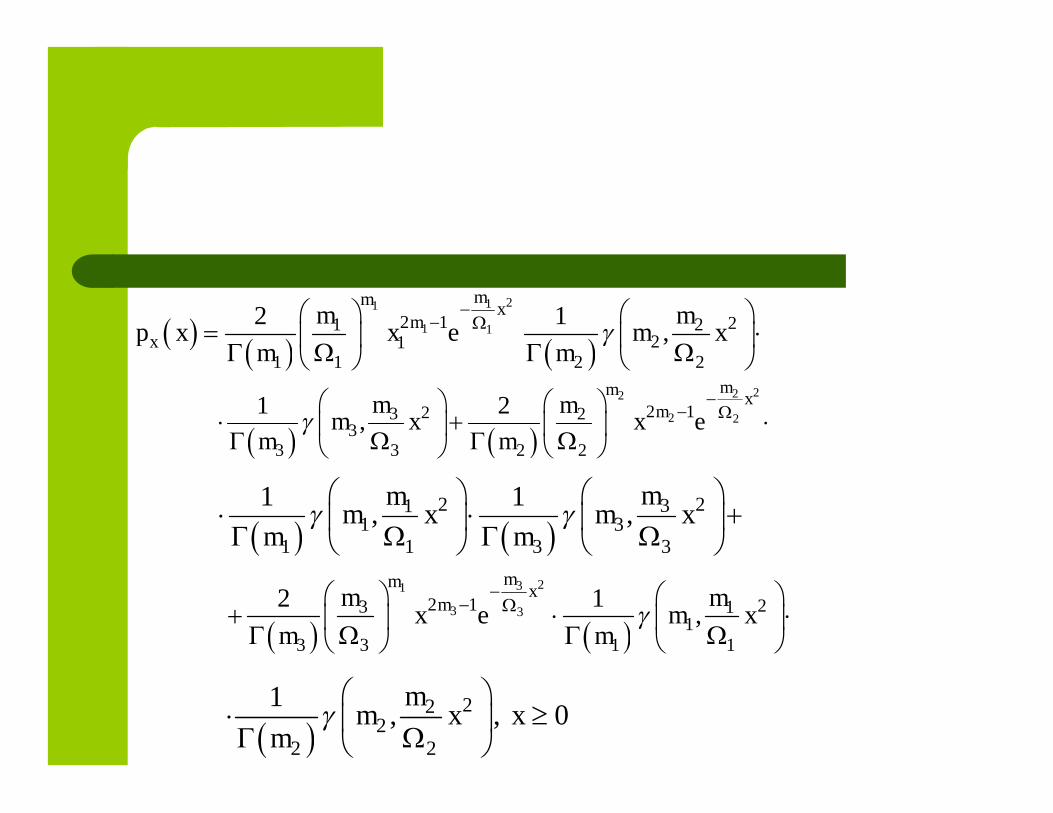
Probability density function (PDF) of x is:

1 2 3x x x xp x p x F x F x

2 1 3 3 1 2x x x x x xp x F x F x p x F x F x

211

1 12 1 21 221

1 1 2 2

2 1,

mmx

mx

m mp x x e m x

m m

222

2 22 123 23

3 3 2 2

1 2,

mmx

mm mm x x e

m m

2 231

1 31 1 3 3

1 1, ,

mmm x m x

m m

231

3 32 1 23 11

3 3 1 1

2 1,

mmx

mm mx e m x

m m

22

22 2

1, , 0

mm x x

m

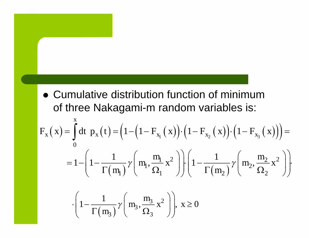
Cumulative distribution function of minimumof three Nakagami-m random variables is:

1 2 3

0

1 1 1 1

x

x x x x xF x dt p t F x F x F x

2 21 2

1 21 1 2 2

1 11 1 , 1 ,

m mm x m x

m m

23

33 3

11 , , 0

mm x x

m

In the previous expressions, parameter m1 isseverity parameter of Nakagami-m fading inthe first section, m2 is severity parameter ofNakagami-m fading in the second sectionand m3 is the severity parameter ofNakagami-m fading in the third section

The Ω1 is signal envelope average power inthe first section, Ω2 is signal envelopeaverage power in the second section and Ω3

is signal envelope average power in the thirdsection

PDF of minimum of three Nakagami-mrandom variables for m1 = m2 =m3 =2

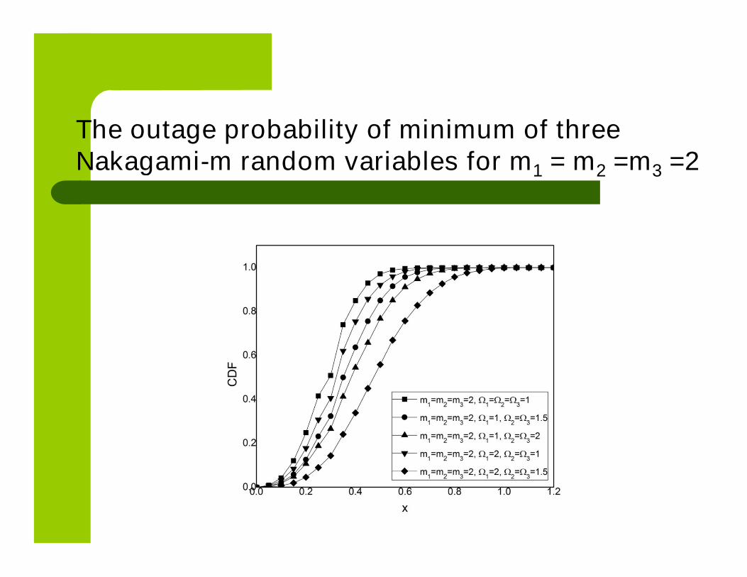
The outage probability of minimum of threeNakagami-m random variables for m1 = m2 =m3 =2

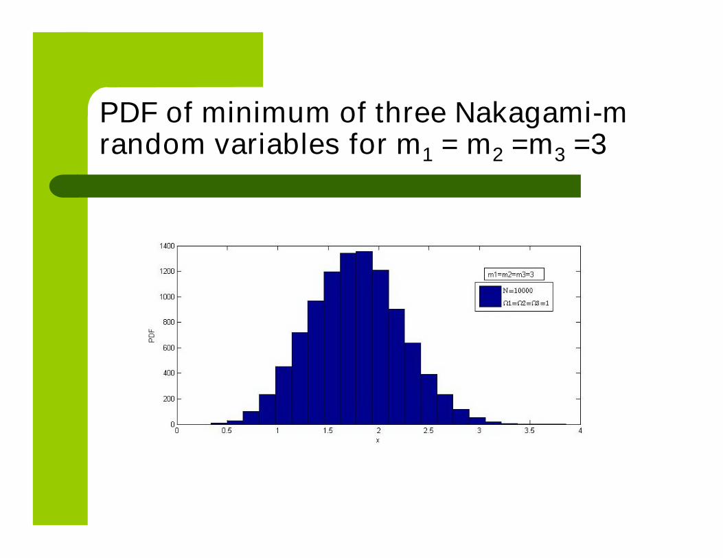
PDF of minimum of three Nakagami-mrandom variables for m1 = m2 =m3 =3

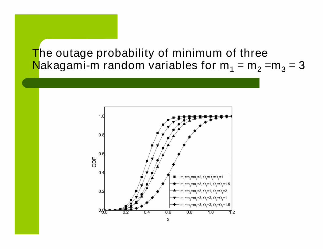
The outage probability of minimum of threeNakagami-m random variables for m1 = m2 =m3 = 3

Probability density functions of x areshown in Figs. 1. and 3 versus of minimumof three Nakagami-m random variables

Severity parameters of Nakagami-m fadingare m1 = m2 =m3 =2 in Fig. 1 andm1=m2=m3 = 3 in Fig. 2

Signal envelope average powers areΩ1=Ω2 = Ω3 =1 in both figures

In Figs. 2 and 4, the outage probabilityin terms of minimum of threeNakagami-m random variables areshown for several values of severityNakagami parameters and severalvalues of signal envelopes averagepowers in sections

The outage probability decreases whenNakagami severity parameter m1 in thefirst section increases, Nakagami severityparameter m2 in the second sectionincreases, and Nakagami severityparameter m3 in the third sectionincreases

Statistics of Product of ThreeNakagami Random Variables

Product of three Nakagami-m random variablesis:

Conditional probability density function of x is:

1 2 3 12 3

,x

x x x x xx x

1

12 3

2 3

/x x

dx xp x x x p

dx x x

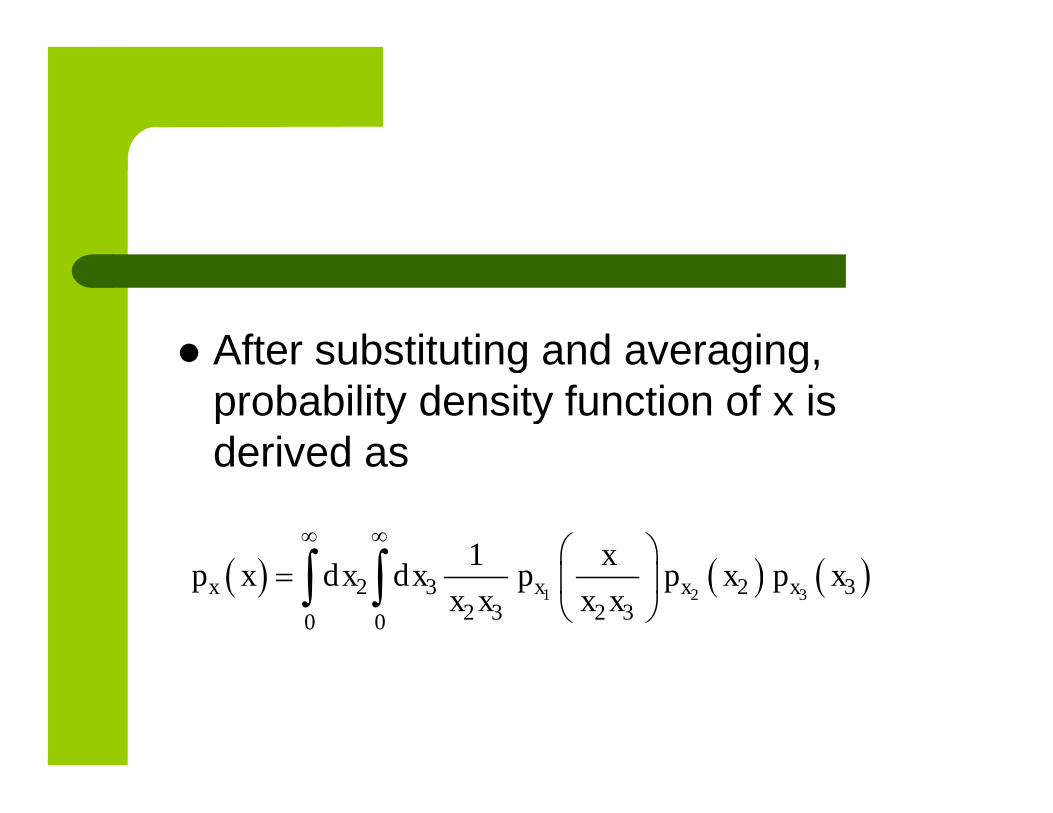
After substituting and averaging,probability density function of x isderived as

1 2 32 3 2 3

2 3 2 30 0

1x x x x

xp x dx dx p p x p x

x x x x

After solving we obtain:

Kn(x) is the modified Bessel function of thesecond kind

31 2

31 2

1 2 3 1 2 3

8mm m

x

mm mp x

m m m

223 12

1 3 1 2 3 2

3 1

22 1 2 2 2 2 11 3 1 3

2 2 22 21 3 1 3 20

2

mm mx

m m m m mm m

m m x mx dx x e K

m x

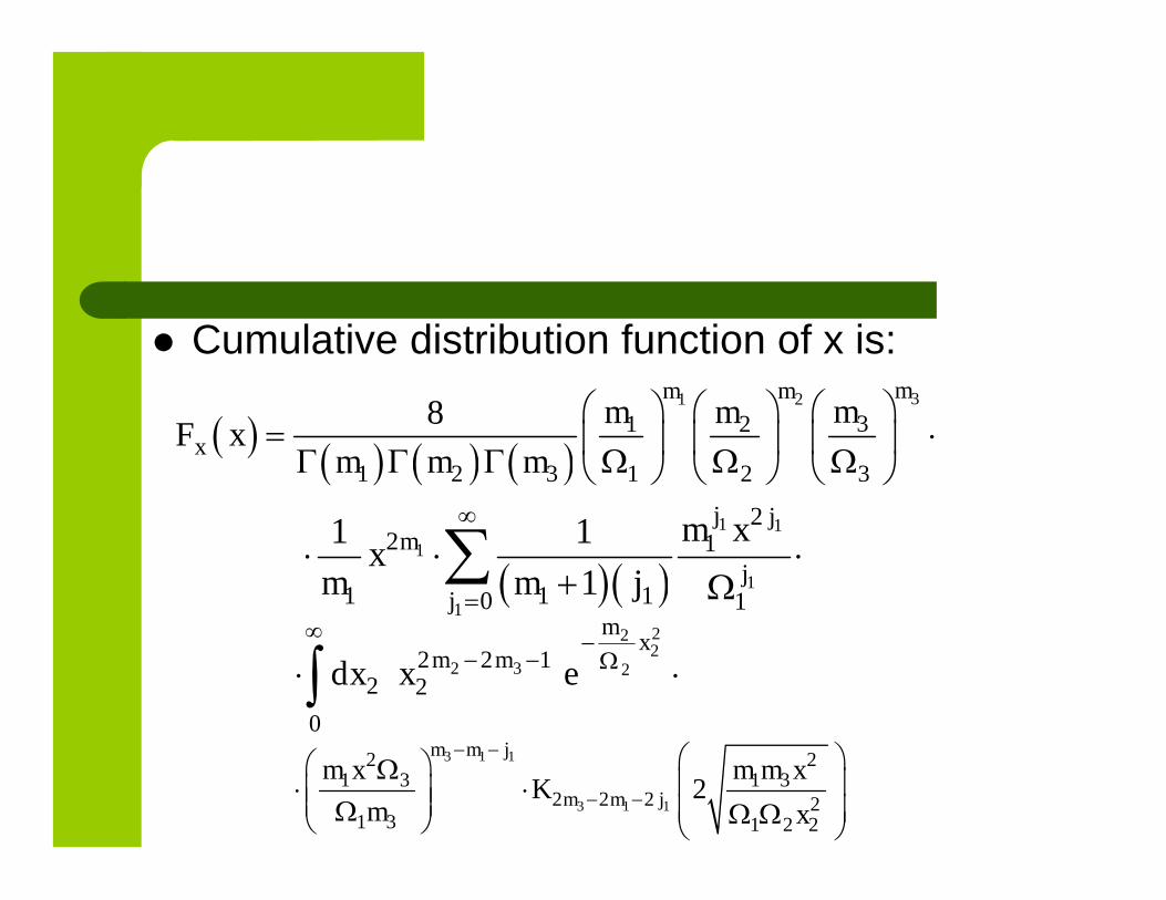
Cumulative distribution function of x is:

31 2

31 2

1 2 3 1 2 3

8mm m

x

mm mF x

m m m

1 1

1

1

1

22 1

1 1 10 1

1 1

1

j jm

jj

m xx

m m j

222

2 3 22 2 12 2

0

mx

m mdx x e

3 1 1

3 1 1

2 21 3 1 3

2 2 2 21 3 1 2 2

2

m m j

m m j

m x m m xK

m x

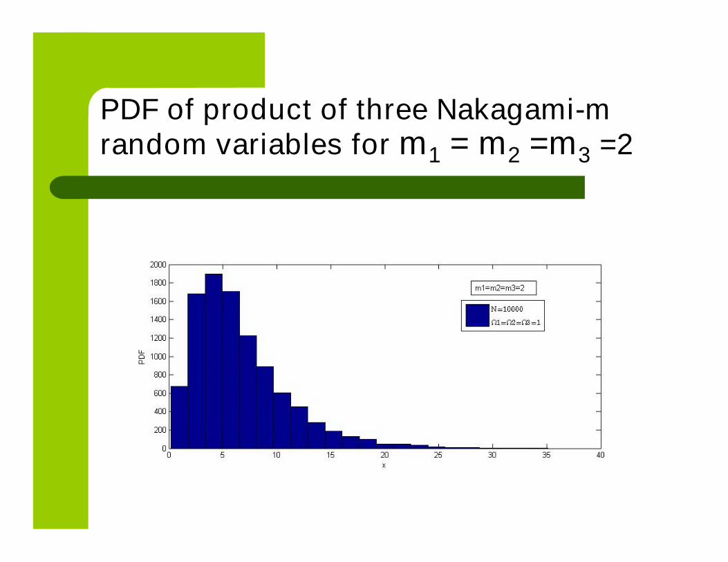
PDF of product of three Nakagami-mrandom variables for m1 = m2 =m3 =2

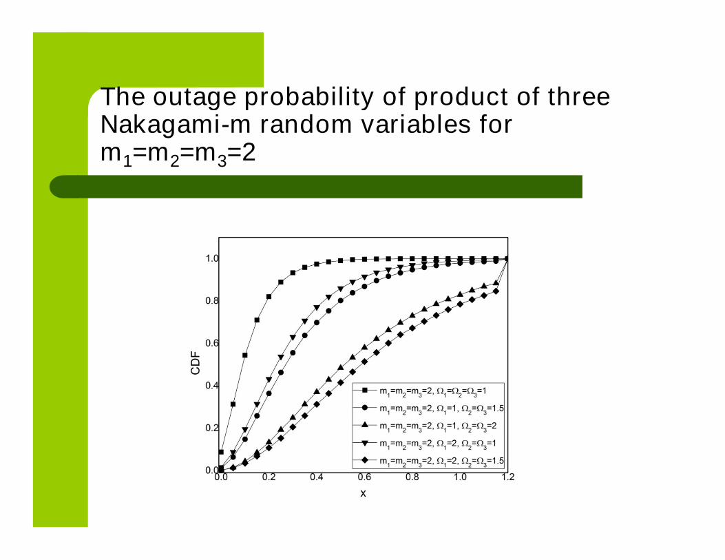
The outage probability of product of threeNakagami-m random variables form1=m2=m3=2

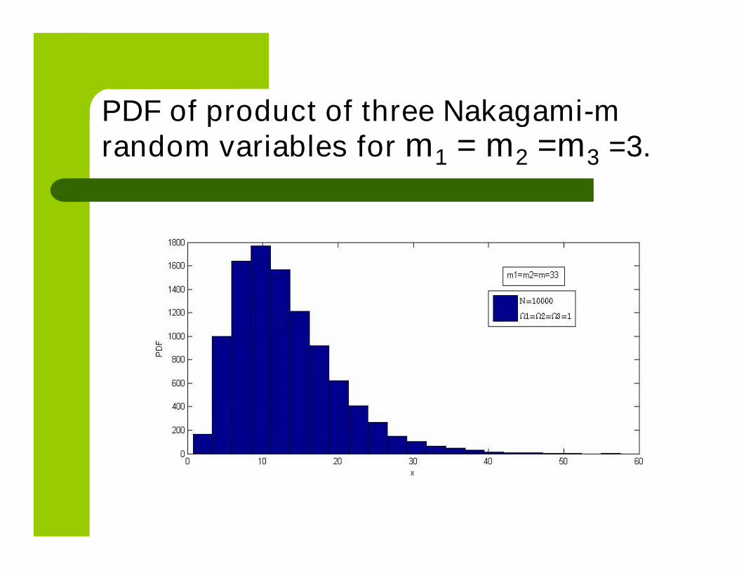
PDF of product of three Nakagami-mrandom variables for m1 = m2 =m3 =3.

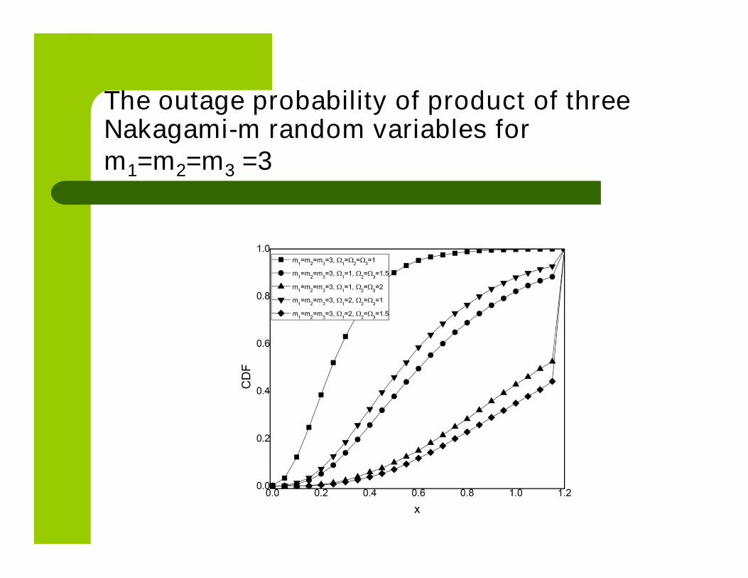
The outage probability of product of threeNakagami-m random variables form1=m2=m3 =3

Probability density functions of x areshown in Figs. 5. and 7 versus of productof three Nakagami-m random variables

Severity parameters of Nakagami-m fadingare m1 = m2 =m3 =2 in Fig. 5 andm1=m2=m3 = 3 in Fig. 7

Signal envelope average powers areΩ1=Ω2 = Ω3 =1 in both figures

In Figs. 6 and 8, the outage probabilitydepending of product of threeNakagami-m random variables isshown for several values of Nakagamiseverity parameters and several valuesof signal envelopes average powers insections

The outage probability decreases whenseverity Nakagami parameter m1 in thefirst section increases, severityNakagami parameter m2 in the secondsection increases, and severityNakagami parameter m3 in the thirdsection increases

Conclusion 4

In this part of Lecture, wireless mobile relayradio communication system with threesections operating over Nakagami-m smallscale fading channel is considered

Nakagami- Nakagami- Nakagami relaychannel is defined

For proposed relay system, the outageprobability is determined

In this work, probability density functions andcumulative distribution functions of minimumof three Nakagami random variables andproduct of three Nakagami random variablesare evaluated

Cumulative distribution function of minimumof three Nakagami random variables isderived in the closed form

Cumulative distribution function of product ofthree Nakagami random variables isobtained as expression with one integral

For both cases, the outage probabilitydecreases when severity parameters ofNakagami fading increase at anysections

These results are useful for designingof wireless mobile relay radiocommunication system with moresections in the presence of gading

Outline

THE FIRST ORDER PERFORMANCE OF PRODUCT

OF THREE RICIAN RANDOM VARIABLES

– PDF of Product of Three Rician RVs

– CDF of Product of Three Rician RVs

– Outage probability of Product of ThreeRician RVs

THE SECOND ORDER PERFORMANCE OF THE

PRODUCT OF THREE RICIAN RANDOM

VARIABLES

– LCR of Product of Three Rician RVs

– AFD of Product of Three Rician RVs

G. K. Karagiannidis, N. C. Sagias, P. T.Mathiopoulos,

“The N * Nakagami Fading Channel Model”

2nd International Symposium on WirelessCommunication Systems, 2005.doi:10.1109/iswcs.2005.1547683

A generic distribution, referred asN*Nakagami, obtained as the product of Nstatistically independent, but not necessarilyidentically distributed, Nakagami-m randomvariables is introduced

The proposed distribution is a convenienttool for analyzing the performance of digitalcommunication systems over generalizedfading channels

The moments-generating function (MGF),PDF, CDF, and moments of the N*Nakagamidistribution are derived in closed-form

Then, closed form expressions for the outageprobability, amount of fading, and averagesymbol error probability for several binaryand multilevel modulation signals of digitalcommunication systems operating over theN*Nakagami fading channel model arepresented

Level Crossing Rate of Wireless RelaySystem with Three Sections Output SignalEnvelope in the Presence of Multipath k-µ

Fading

Dragana Krstic,

Danijela Aleksic, Goran Petkovic,

Ivica Marjanovic Mihajlo Stefanovic

In this part of work, the wireless relay systemwith three sections in the presence ofmultipath k-µ fading is presented

The useful closed form expression for theaverage Level Crossing Rate (LCR) iscalculated

The resulting integrals are solved by usingthe Laplace approximating formula for tworandom variables

Product of three k-µ random variables x1, x2

and x3 is:

x1, x2 and x3 are independent

Then it is valid:

321 xxxz

321

xx

zx

The first derivative of product of three k-µrandom variables x1, x2 and x3 is:

The first derivative of k-µ random process isGaussian distributed

The linear combination of Gaussian randomprocesses is Gaussian random process.

321231132 xxxxxxxxxz

Therefore, the first derivative of product ofthree k-µ random variables has conditionalGaussian distribution

The main of is zero

The variance of is:

z

z

222

21

223

21

223

22

2321 xxxz xxxxxx

Here:

fm is maximal Dopler frequency

Ωi, i=1, 2, 3, are power of k-µ randomvariables and

µ is severity of k-µ fading

2 2 2

1i

ix mf

k

The joint probability density function of z, ,x2 and x3 is:

and:

z

323232 3232/ xxzpxxzzzpxxzzp xzxzxxzz

323232 //32

xxzpxpxpxxzzzp zxxz

32

132 1

/xx

zp

dz

dxxxzp xz

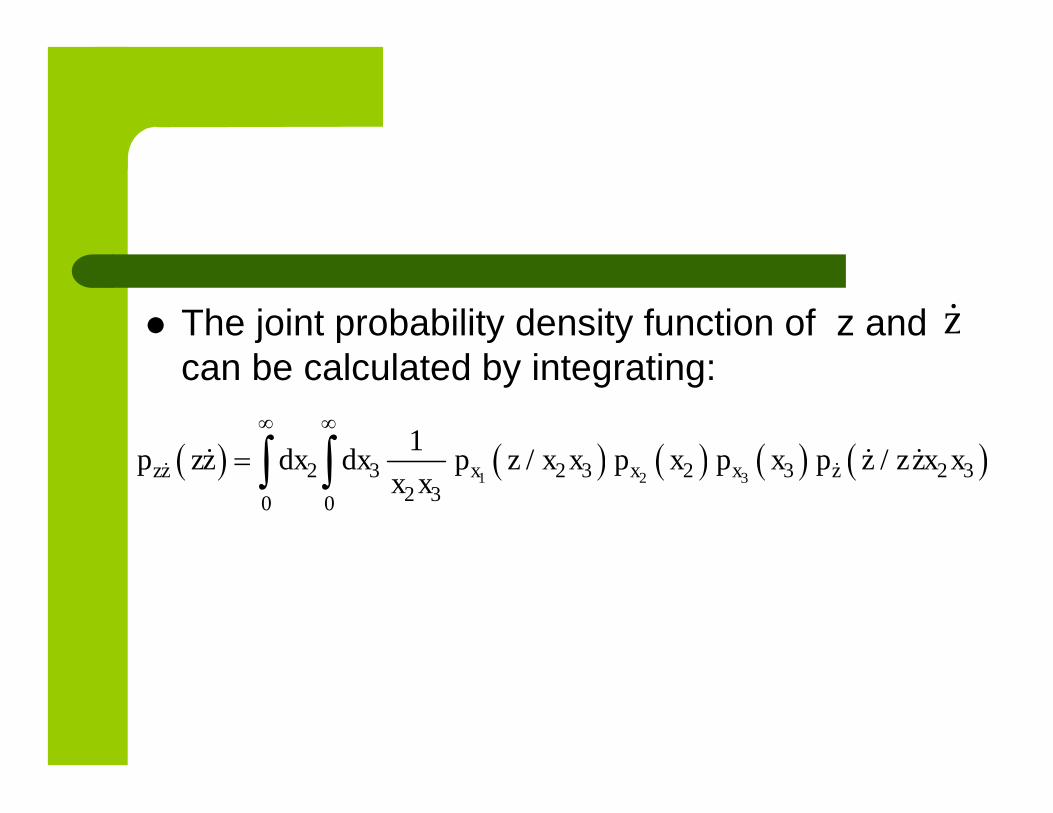
The joint probability density function of z andcan be calculated by integrating:

z

1 2 32 3 2 3 2 3 2 3

2 30 0

1/ /zz x x x zp zz dx dx p z x x p x p x p z z zx x

x x

The level crossing rate of product of three k-µ randomprocesses can be calculated as average value of the firstderivative of product of three k-µ random processes:

1 2 32 3 2 3 2 3

2 30 0 0

1/z zz x x xN dz zp zz dx dx p z x x p x p x

x x

1 2 32 3 2 3 2 3 2 3

2 30 0 0

1/ /

2

zz x x xdz z p z z x x dx dx p z x x p x p x

x x

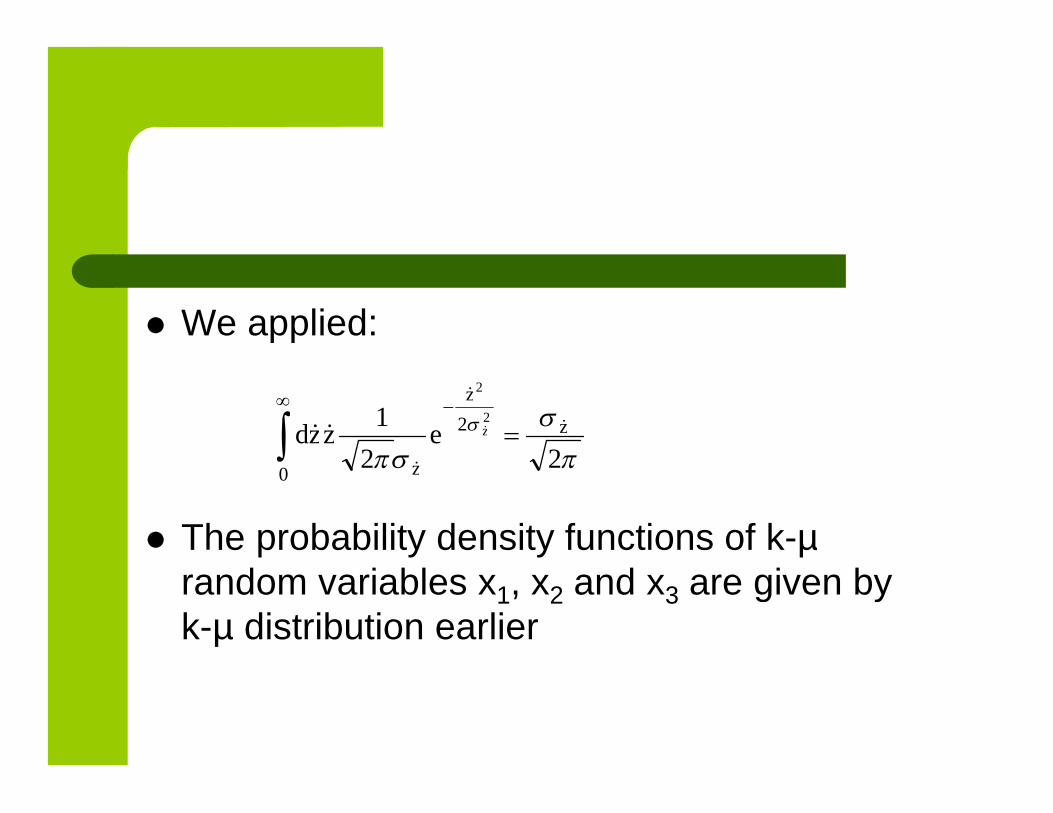
We applied:

The probability density functions of k-µrandom variables x1, x2 and x3 are given byk-µ distribution earlier

22

1 2

2

2

0

z

z

z

zezzd

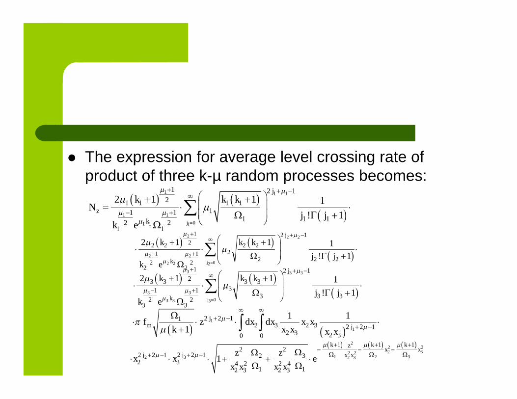
The expression for average level crossing rate ofproduct of three k-µ random processes becomes:

1 1 1

1 1

01 1 1

1 2 121 1 1 1

11 11 1 1

2 21 1

2 1 1 1

! 1j

j

z

k

k k kN

j jk e

2 2 2

2 2

02 2 2

1 2 122 2 2 2

21 12 2 2

2 22 2

2 1 1 1

! 1j

j

k

k k k

j jk e

3 3 3

3 3

03 3 3

1 2 123 3 3 3

31 13 3 3

2 23 3

2 1 1 1

! 1j

j

k

k k k

j jk e

1

1

2 2 112 3 2 3 2 2 1

2 3 2 30 0

1 1

1j

m jf z dx dx x x

k x x x x

2

2 22 32 2

1 2 332 2 3

1 1 12 2

2 2 12 2 1 322 3 4 2 2 4

1 12 3 2 3

1

k k kzx x

jj x xz zx x e

x x x x

The integral J is:

1

343

22

2

1

223

42

22222

0

3

0

2 113

3

12

2 xx

z

xx

zxxdxdxJ jjjj

2

33

22

223

22

2

1

111x

kx

k

xx

zk

e

1

343

22

2

1

223

42

2

0

3

0

2 1xx

z

xx

zdxdx

31321223

3

22

223

22

2

1

ln22ln22111

xjjxjjxk

xk

xx

zk

e

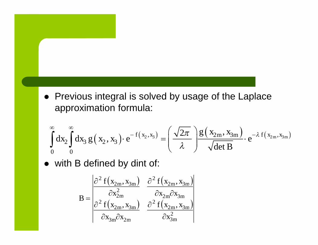
Previous integral is solved by usage of the Laplaceapproximation formula:

with B defined by dint of:

2 3 2 3, ,2 32 3 2 3

0 0

,2,

detm mf x x f x xm mg x x

dx dx g x x e eB

23

322

23

322

32

322

22

322

,,

,,

m

mm

mm

mm

mm

mm

m

mm

x

xxf

xx

xxf

xx

xxf

x

xxf

B

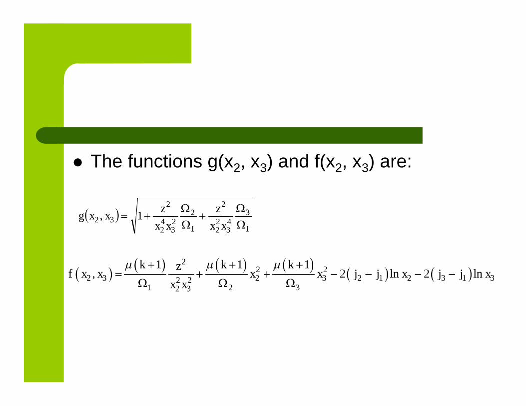
The functions g(x2, x3) and f(x2, x3) are:

1

343

22

2

1

223

42

2

32 1,

xx

z

xx

zxxg

2

2 22 3 2 3 2 1 2 3 1 32 2

1 2 32 3

1 1 1, 2 ln 2 ln

k k kzf x x x x j j x j j x

x x

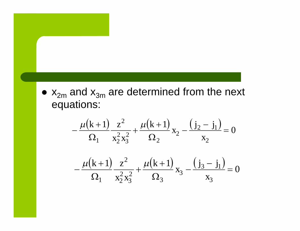
x2m and x3m are determined from the nextequations:

0

11

2

122

223

22

2

1

x

jjx

k

xx

zk

0

11

3

133

323

22

2

1

x

jjx

k

xx

zk

In Fig. 1, the normalized average levelcrossing rate of product of three k-µ randomprocesses is presented

The family of curves is shown for severalvalues of Rician factor, k-µ fading parameterµ and average signal envelope powers atsections, Ω

Rician factor k and fading parameter µ areequal to 1 in all cases

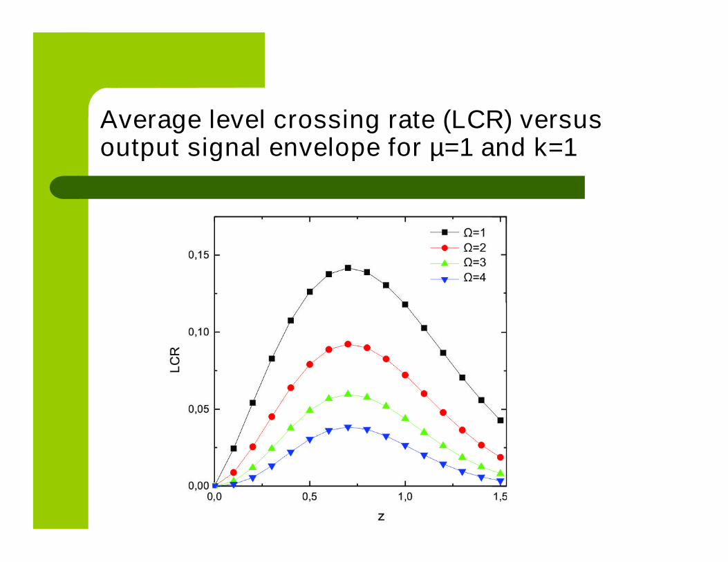
Average level crossing rate (LCR) versusoutput signal envelope for µ=1 and k=1

Signal envelope powers are variable

It is visible from this graph that average levelcrossing rate increases when average signalenvelope power decreases

The influence of average signal envelopepower on average level crossing rate ishigher for lower values of average signalenvelope power

Average level crossing rate (LCR) versusoutput signal envelope for Ω=1 and µ=1

In this Figure, the normalized average level crossingrate of product of three k-µ random processes isshown for several values of Rician factor k, whileparameter µ and average signal envelope power Ω have constant values: µ=1 and Ω=1 for all curves

It can be seen from this figure that average LCRincreases with decreasing of Rician factor

The influence of Rician factor on average LCR ishigher for lower values of Rician factor k

Conclusion 5

By this result, average level crossing rate ofproduct of three Nakagami-m randomprocesses or average level crossing rate ofproduct of three Rician random processescan be evaluated

Average level crossing rate can be used forevaluation the average fade duration (AFD)of relay system with three sections in thepresence of k-µ multipath fading

The system performance is better for lowervalues of average level crossing rate

The average level crossing rate decreaseswhen Rician factor increases, dominantcomponent power increases and scatteringcomponents power decreases

For higher values of parameter µ averagelevel crossing rate has lower values andoutage probability decreases

When average power at sections increases,average level crossing rate decreases

The numerical expressions show theinfluence of Rician factor, k-µ multipathfading parameter µ and average powers onaverage LCRof product of three k-µ randomprocesses

The expression for the LCR can be used forcalculating the average fade duration of theproposed relay system

Outage Probability of Two RelaySystems with Two Sections on

Selection Combining in thePresence of κ-μ Short Term Fading

Dragana KrstićDanijela AleksićSiniša MinićMihajlo StefanovićVladeta MilenkovićDjoko Bandjur

Two wireless relay communication systemswith two sections on selection combining(SC) are considered in this part of Lecture

Received signal in sections experiences κ-μsmall scale fading

Signal envelope at output of relay systemscan be evaluated as product of signalenvelopes in sections

The probability density function (PDF) andcumulative distribution function (CDF) at outputof relay system are calculated

SC receiver selects relay system with highersignal envelope at its inputs

Thus, PDF and CDF of SC receiver signalenvelope are calculated by solving integrals inthe closed forms by using sums and Besselfunction of the second kind

Then, they are graphically presented

The influence of Rician factors of κ-μ shortterm fading in sections and κ-μ short termfading severity parameters on the outageprobability of considered relay system isanalyzed and discussed

These results serve to designers of wirelesssystems to choose optimal system parametersin appropriate fading environment

Introduction

Here, two relay systems on selectioncombining (SC) receiver are considered

Such relay system has two sections

Received signal in each section is subjectedto κ-μ short term fading

Signal envelope at output of proposedwireless relay system can be evaluated asmaximum of two signal envelopes at outputsof relay systems

In this part, two wireless relay communication systemswith two sections and with SC receiver in the presenceof κ-μ short term fading in sections are studied

Signal envelopes at output of relay systems can bewritten as product of two κ-μ random variables

Therefore, probability density function and cumulativedistribution function of product of two κ-μ randomvariables with different parameters are evaluated

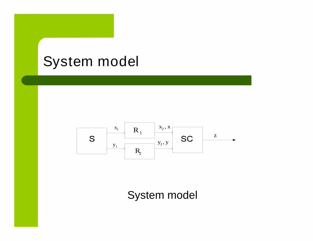
System model

System model

1x

1y

z1R

2R

2 ,x x

2 ,y y

System model

In this paper, the wireless relaycommunication mobile radio system with SCreceiver is considered

Model of proposed system is shown inprevious Figure

The signal envelopes x1 and x2 follow κ-μdistribution:

2

1

12

1

1

2

1

11

1

11

1

11

12i

ii

i

ii

i

ik

i

iiiix

ek

xkxp

1 1 2

1

1

1

1 11 1 1

1

12

i ii

i

i

kx

i ii i

i

k ke I x

By solving we have:

1

1 1

1 1

1

21 1

1 1

2 21 1

2 1i

i i i

i i

i ix i

ki i

kp x

k e

1 1

1

2 1

1 11

1 1 1 10

1 1

!

ik

i ii

i ik

k k

k k

2,1,0,22

1

11

11

1

122

ixex i

xk

ki

i

ii

i

Random variables y1 and y2, also, follow κ-μdistribution:

2

1

22

1

2

2

1

22

2

22

2

2

12i

ii

i

i

i

ik

i

iiiy

ek

kyp

ik

k

i

iii

kk

kki

2220

12

2

222

!

11

2

22

2,1,0,22

2

22

22

1

122

iyey i

xk

ki

i

ii

i

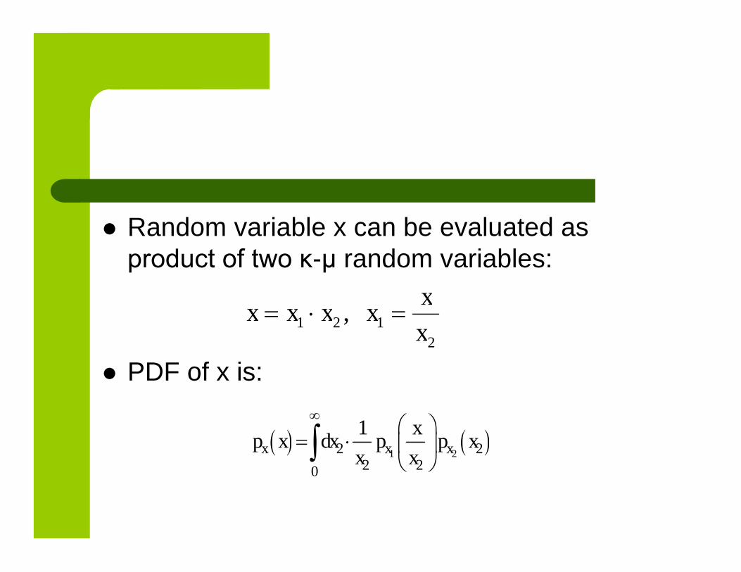
Random variable x can be evaluated asproduct of two κ-μ random variables:

PDF of x is:

2

121 ,x

xxxxx

1 22 2

2 20

1x x x

xp x dx p p x

x x

After solving we have:

Here, Kn(x) is the modified Bessel function of thesecond kind with argument x and order n

11

11 11

11 11

1

211 11

1 1

2 211 11

2 1x

k

kp x

k e

121 11

11 1

12 12

1 12 12

12 1211 11 12 122 2 1

11 1 11 1 11110 2 2

12 12

1 2 11

!

k

k

k k

k k kx

k kk e

12 2 11 1

12 2 11 1

2 22 2 2 211 11 11 11 12 1212

11 12 12 11 12

1 1 112

2 1

k k

k k

k x k x kK

k

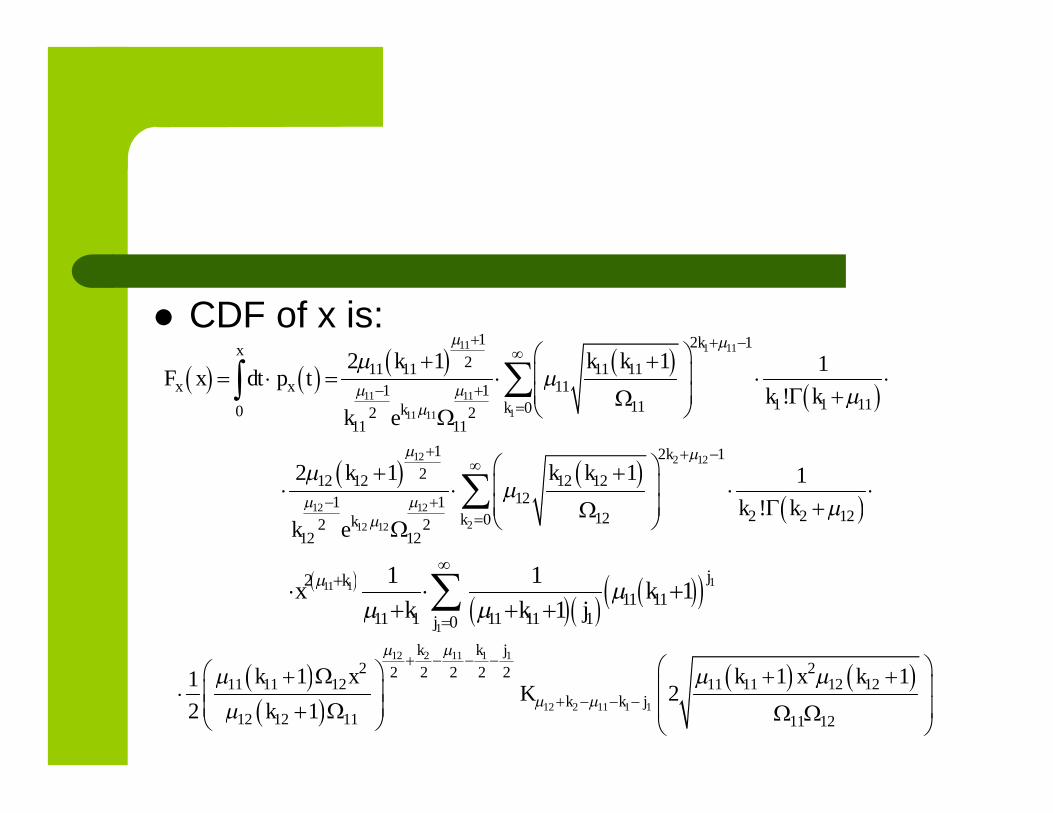
CDF of x is:

11 1 11

11 11

111 11

1 2 1211 11 11 11

111 11 1 111100 2 2

11 11

2 1 1 1

!

kx

x x

kk

k k kF x dt p t

k kk e

12 2 12

12 12

212 12

1 2 1212 12 12 12

121 12 2 121202 2

12 12

2 1 1 1

!

k

kk

k k k

k kk e

111 1

1

211 11

11 1 11 11 10

1 11

1

jk

j

x kk k j

12 2 11 1 1

12 2 11 1 1

2 22 2 2 2 211 11 12 11 11 12 12

12 12 11 11 12

1 1 112

2 1

k k j

k k j

k x k x kK

k

Similarly, the PDF of y is:

21 3 21

21 21

321 21

1 2 1221 21 21 21

211 13 3 212102 2

21 21

2 1 1 1

!

k

y

kk

k k kp y

k kk e

22 4 22

3 21

22 22

422 22

1 2 1222 22 22 22 2 2 1

221 14 4 222202 2

22 22

2 1 1 1

!

k

k

kk

k k ky

k kk e

322 4 21

22 4 21 3

2 22 2 2 221 21 22 21 21 22 22

21 22 22 21 22

1 1 112

2 1

kk

k k

k y k y kK

k

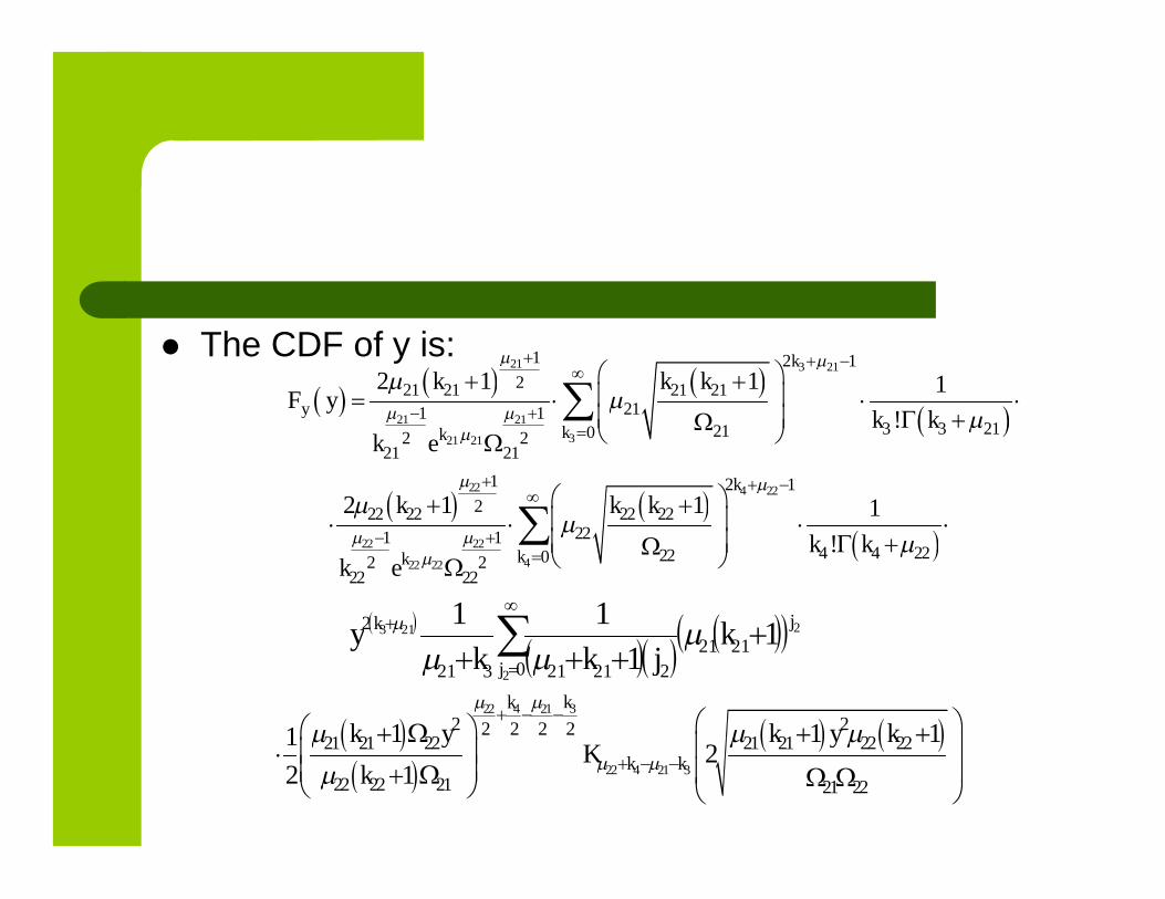
The CDF of y is:

21 3 21

21 21

321 21

1 2 1221 21 21 21

211 13 3 212102 2

21 21

2 1 1 1

!

k

y

kk

k k kF y

k kk e

22 4 22

22 22

422 22

1 2 1222 22 22 22

221 14 4 222202 2

22 22

2 1 1 1

!

k

kk

k k k

k kk e

2

2

213 11

112121

0 22121321

2 j

j

k kjkk

y

322 4 21

22 4 21 3

2 22 2 2 221 21 22 21 21 22 22

22 22 21 21 22

1 1 112

2 1

kk

k k

k y k y kK

k

The outage probability is probability thatcommunication relay system output signalenvelope drops below the defined threshold

The outage probability for this case is equalto the CDF of product of signal envelopes atsections

The CDF of SC ReceiverOutput Signal

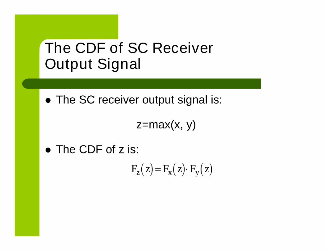
The SC receiver output signal is:

z=max(x, y)

The CDF of z is:

z x yF z F z F z

After solving it is valid:

11 1 11

11 11

111 11

1 2 1211 11 11 11

111 11 1 111102 2

11 11

2 1 1 1

!

k

z

kk

k k kF z

k kk e

12 2 12

12 12

212 12

1 2 1212 12 12 12

121 12 2 121202 2

12 12

2 1 1 1

!

k

kk

k k k

k kk e

111 1

1

211 11

11 1 11 11 10

1 11

1

jk

j

z kk k j

12 2 11 1

12 2 11 1

2 22 2 2 211 11 12 11 11 12 12

12 12 11 11 12

1 1 112

2 1

k k

k k

k z k z kK

k

21 3 21

21 21

321 21

1 2 1221 21 21 21

211 13 3 212102 2

21 21

2 1 1 1

!

k

kk

k k k

k kk e

22 4 22

22 22

422 22

1 2 1222 22 22 22

221 14 4 222202 2

22 22

2 1 1 1

!

k

kk

k k k

k kk e

2

2

213 11

112121

0 22121321

2 j

j

k kjkk

z

322 4 21

22 4 21 3

2 22 2 2 221 21 22 21 21 22 22

22 22 21 21 22

1 1 112

2 1

kk

k k

k z k z kK

k

Numerical results

The probability density function of SC receiveroutput signal envelope is plotted in next Figuresfor some values of fading severity parameter μand Rician factors

In the first Figure, fading severity parameter μ=2and Rician factors are kij=1; i, j = 1, 2

In the second one, fading severity parameter μ=3and Rician factors are kij=2; i, j = 1, 2

Fig. 2. PDF of x for μ=2 and kij=1

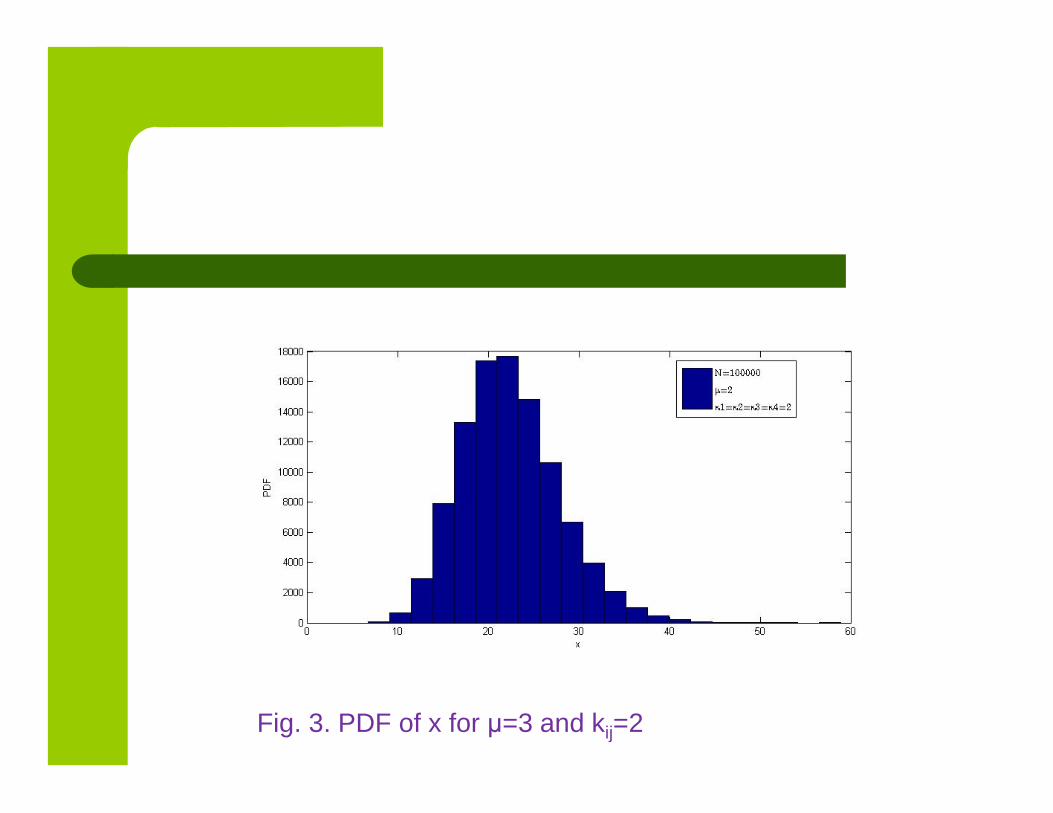
Fig. 3. PDF of x for μ=3 and kij=2

The cumulative distribution functions of SCreceiver output signal envelope are plotted inthe next few Figures for different quantities offading severity parameter μ and Ricianfactors

In first some figures, parameter μ=2, and inlast two, fading severity parameter μ=3

The CDF is plotted for variable parameters κ

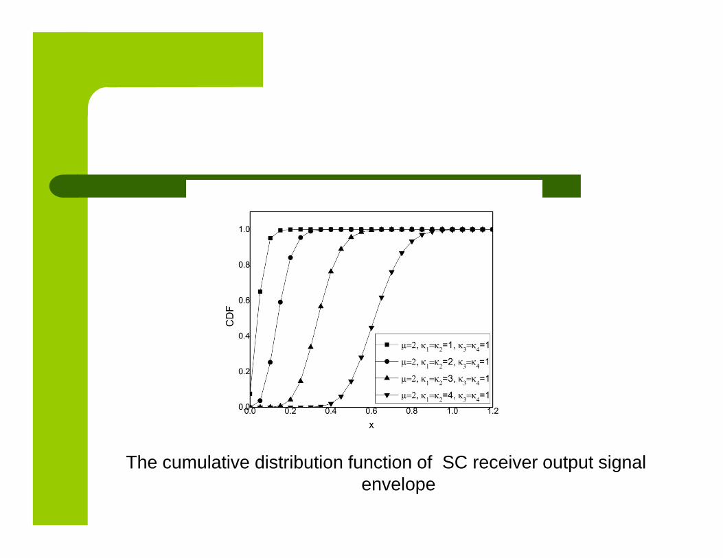
The cumulative distribution function of SC receiver output signalenvelope

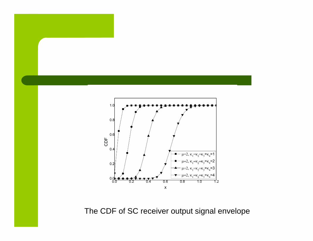
The CDF of SC receiver output signal envelope

The cumulative distribution function of SC receiver output signalenvelope

It is visible that CDF increases with increasingof the signal envelope

The cumulative distribution function decreasesfor larger values of Rician factor κij

Also, one can see from these figures that CDFis smaller for bigger values of fading severityparameter μ

System performances are better for lowervalues of the outage probability

Conclusion 6

In this article, wireless system with two relaycommunication systems, both with two sections,whose outputs are inputs in SC receiver, in thepresence of κ-μ short term fading in sections, isstudied

Signal envelopes at output of relay systems areproducts of two κ-μ random variables

The probability density function and cumulativedistribution function of products of two κ-μ random

variables with different parameters are evaluated

The signal envelope at output of proposedsystem is presented as maximum of signalenvelopes at outputs of relay systems

Then, probability density function, cumulativedistribution function and outage probability ofconsidered system are determined and theinfluence of Rician factors at sections onoutage probability is analyzed and discussed

More references:

A. Panajotović, N. Sekulović, A. Cvetković, D. Milović,“System performance analysis of cooperative multihoprelaying network applying approximation to dual-hoprelaying network”, International Journal ofCommunication Systems, 2020, e4476.

doi:10.1002/dac.4476

.

Any questions or comments

please email me:

dragana.krstic@elfak.ni.ac.rs

dragana.krstic_elfak_ni@yahoo.com