Determinants of Agricultural Productivity in Kenya

Determinants of Agricultural Productivity in Kenya.

By

Beth Wanjiru Muraya

X50 / 74809 / 2014

A Research Project Submitted In partial Fulfilment for the award of the Degree of Master

of Arts in Economics, of the The University of Nairobi.

April, 2017

I | P a g e

DECLARATION

This project is my original work and has not been presented for a degree in any other University

…………………………………….. ……………………………………...

Signature Date

Beth Wanjiru Muraya

This project was submitted for examination with my approval as University Supervisor

…………………………………….. ……………………………………...

Signature Date

Dr. George Ruigu

II | P a g e

DEDICATION

To God Almighty, from whom all good things come.

III | P a g e

ACKNOWLEDGEMENT

Special thanks to everybody who has played a role in the coming to fruition of this project.

I am thankful to my supervisor, Dr. George Ruigu. I thank you for your endless guidance,

unyielding support and relentless efforts to always hold me to a higher standard of output and for

tapping into my intellectual curiosity.

I am thankful to my family members- My Father Muraya, mother Wanjiku, my brothers Michuki

& Kariuki and my sister Njoki- for their unfathomable support the entire period of my graduate

studies.

I also acknowledge my friends and classmates, Nashon, Ndungu and Michael, for journeying with

me and always provoking my intellectual curiosity.

Above all, to Almighty God, I bow in adulation.

To you all, I salute in appreciation.

IV | P a g e

ABBREVIATIONS

ASALs Arid and semiarid lands

TFP Total factor productivity

PFP Partial factor productivity

Trans log Transcendental logarithm

OLS ordinary least square technique

KALRO Kenya Agricultural and Livestock Research Organization

SRA Strategy for Revitalizing Agriculture

ASDC Agricultural Sector Development Strategy

V | P a g e

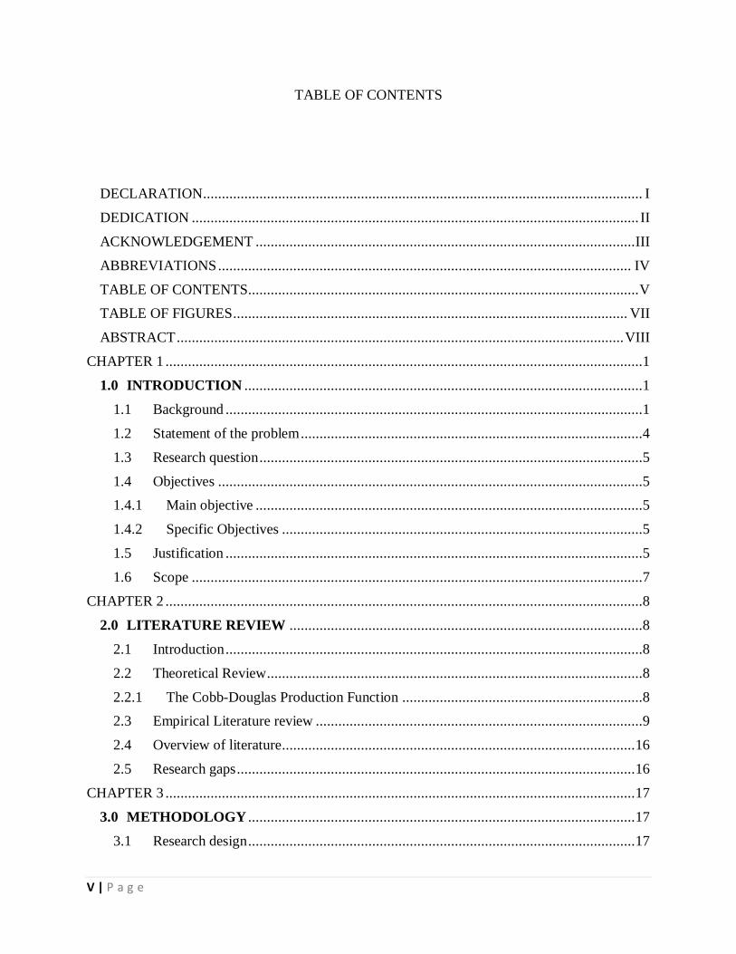
TABLE OF CONTENTS

DECLARATION ..................................................................................................................... I

DEDICATION ....................................................................................................................... II

ACKNOWLEDGEMENT ..................................................................................................... III

ABBREVIATIONS .............................................................................................................. IV

TABLE OF CONTENTS ........................................................................................................ V

TABLE OF FIGURES ......................................................................................................... VII

ABSTRACT ....................................................................................................................... VIII

CHAPTER 1 ...............................................................................................................................1

1.0 INTRODUCTION ..........................................................................................................1

1.1 Background ...............................................................................................................1

1.2 Statement of the problem ...........................................................................................4

1.3 Research question ......................................................................................................5

1.4 Objectives .................................................................................................................5

1.4.1 Main objective .......................................................................................................5

1.4.2 Specific Objectives ................................................................................................5

1.5 Justification ...............................................................................................................5

1.6 Scope ........................................................................................................................7

CHAPTER 2 ...............................................................................................................................8

2.0 LITERATURE REVIEW ..............................................................................................8

2.1 Introduction ...............................................................................................................8

2.2 Theoretical Review ....................................................................................................8

2.2.1 The Cobb-Douglas Production Function ................................................................8

2.3 Empirical Literature review .......................................................................................9

2.4 Overview of literature .............................................................................................. 16

2.5 Research gaps .......................................................................................................... 16

CHAPTER 3 ............................................................................................................................. 17

3.0 METHODOLOGY ....................................................................................................... 17

3.1 Research design ....................................................................................................... 17

VI | P a g e

3.2 Conceptual framework............................................................................................. 17

3.3 Data sources ............................................................................................................ 20

3.4 Data processing and Analysis .................................................................................. 20

CHAPTER 4 ............................................................................................................................. 21

4.0 DATA ANALYSIS, FINDINGS, AND DISCUSSION ................................................ 21

4.1 Method of Analysis ................................................................................................. 21

4.2 Empirical Findings .................................................................................................. 22

4.3 Discussion of results ................................................................................................ 27

CHAPTER 5 ............................................................................................................................. 30

5.0 SUMMARY, CONCLUSION AND RECOMMENDATIONS ................................... 30

5.1 Summary ................................................................................................................. 30

5.2 Conclusion .............................................................................................................. 31

5.3 Policy Recommendations ........................................................................................ 32

REFERENCES ......................................................................................................................... 33

VII | P a g e

TABLE OF FIGURES

Table 4. 1 Dickey-Fuller test for unit root .................................................................................. 23

Table 4. 2 Cointegration Rank for determinants of agricultural productivity, (1980-2013) ....... 23

Table 4. 3 Error Correction Model Equations (ECM) ................................................................ 26

Table 4. 4 OLS estimates 1980-2013 ......................................................................................... 27

VIII | P a g e

ABSTRACT

This study sought to identify the determinants of agricultural productivity in Kenya. The study

used partial factor productivity given by physical output over factor inputs. It explored inflation,

real exchange rate, labour force, government expenditure and climate/rainfall as the factors

determining agricultural productivity. The study utilized secondary data for the period of 1980 to

2013. The study employed Cobb-Douglas production function and ordinary least square (OLS)

estimation technique as the method of analysis. The independent variables were labour force,

inflation, real exchange rate, government expenditure and climate/rainfall while the dependent

variable was agricultural productivity.

From the regression results, an increase of one percent in government expenditure, annual rainfall,

labour force caused an increase in agricultural productivity by 0.0639032%, 0.0917103%,

0.1984402% respectively. An increase of one percent in inflation rate, exchange rate in caused a

decrease in agricultural productivity by 0.0193286% and 0.405422% respectively. Overall the

model is statistically significant at 5% level of significance.

The study also employed Johansen-Granger Cointegration procedures and Error Correction Model

(ECM) to forecast long-run relationships and to check for short-run relationship respectively

among the study variables. The long run relation highlights the negative impact of exchange rate

(E) and inflation (I) on agricultural productivity (Y), while Labour force, rainfall, and government

expenditure impact agricultural productivity positively.

From the results of Error Correction Model, labour, rainfall and government expenditure have a

high explanatory power, as indicated by R2 of 0.9105, 0.7181 and 0.6613 respectively. Exchange

rate and inflation rate have a relatively low explanatory power given by R2 of 0.3231 and 0.3204

respectively. This implies that in the short run Labour, rainfall, and government expenditure are

the main determinants of agricultural productivity in Kenya.

1 | P a g e

CHAPTER 1

1.0 INTRODUCTION

1.1 Background

Agriculture is the backbone of Kenya’s Economy. The contribution of the sector to the country’s

Gross Domestic Product (GDP) has been declining over the years from 40 percent in 1963, 33

percent in the 1980s to 27 percent in 2014, (KNBS, 2015). The sector, however, remains the

dominant sector in the overall economy. The sector accounts for about 60 percent of the foreign

exchange in Kenya, about 16 percent of the formal sector employment (KNBS, 2015) and also

provides self-employment. There is, therefore a high correlation between the growth of the national

economy and development in the agricultural sector.

About 15 percent of the Kenyan total land area is fertile and has sufficient rainfall to support

farming but only about a third of the land is grouped as first-class land for agriculture purpose.

Subsistence production accounts for almost half of the total agricultural production which is both

marketed and non-marketed.

According to the economic pillar of Vision 2030, Kenya seeks to achieve a sustainable growth of

10 percent annually. This will be crucial in generating more resources so as to achieve the

sustainable development. Vision 2030 identified agriculture as a critical sector to achieve the 10

percent growth rate (Government of Kenya, 2007).

In 2004 the government of Kenya launched the Strategy for Revitalizing Agriculture (SRA). This

provided a guide to both private and public sectors on how to overcome the challenges in the

agricultural sector. This strategy was largely successful as the agricultural sector achieved a growth

of 6.1% in 2007 (Government of Kenya, 2010). The Agricultural Sector Development Strategy

2 | P a g e

(ASDS) succeeded SRA. It aims at achieving annual growth rate of 10% in the agricultural sector

thus complementing Vision 2030. Under ASDS agricultural sector should employ contemporary

methods and technologies so as to modernize agriculture and enhance productivity. The

government should also ensure that institutions providing services to farmers are more effective

and efficient.

According to Vision 2030, Productivity is still a cardinal challenge in the agricultural sector. The

level has either remained nearly constant over the last five years or is on decline. The production

level of most crops over the last five years has almost stagnated or has been declining. Fish and

livestock products output levels are below potential. Population growth has been steadily

increasing while the area covered by the forest has been sharply reducing. Over the years tree

productivity has been dwindling (Government of Kenya, 2007).

Land use is another challenge in the agricultural sector. The land available for crop production is

overexploited especially the small-scale farmers in Kenya. Arid and semi-arid lands (ASALs) and

land in high and medium potential areas remain underexploited for agricultural production in

Kenya.

Kenyan Agricultural sector has continued to rely heavily on rain-fed agriculture. However, this

has been an area of concern, due to the effects of global warming; climate is not very predictable

coupled with natural disasters like drought, floods, and mudslides. There is a close relationship

between rainfall and agricultural output as it affects productivity in many counties in Kenya. Only

about a third of Kenyan land is agricultural land (World Bank Group, 2015). Agricultural land, in

this case, is described as the share of land that is arable and under permanent crop and pasture.

Thus there is a huge variability in production by region in Kenya based on whether the region

receives adequate rainfall or not. However, if irrigation is adopted across the country this could

3 | P a g e

greatly reduce the regional variability of productivity. This is, however, subject to irrigation

potential of different regions as well as budget constraints due to the high costs involved in

establishing irrigation schemes. The climatic condition affects policies as well as the use of inputs

which has a direct impact on productivity.

Planned irrigation in the agricultural sector in Kenya began in 1946. This was at the time when

African Land Development (ALDEV) was trying to contain people from encroaching on the white

settlements. The National irrigation board (NIB) was consequently established in 1966. The NIB

is currently managing Bunyala, Hola, Mwea, Ahero, Bura, Perkerra and West Kano irrigation

schemes. The government has also recently embarked on Galana-Kulalu Food Security Project in

Kilifi and Tana counties. All these projects aim at enhancing food security.

Value addition is critical to making agricultural products more competitive in the global market as

well as earn farmers the maximum returns. Farmers in Kenya export semi-processed agricultural

products which are often low in value. These semi-processed exports form a significant percentage

(about 91%) of the entire agricultural related exports. Relatively high production costs and

inability to add value to the agricultural output makes Kenyan agricultural exports less competitive

globally.

Government expenditure can directly or indirectly affect agricultural incomes. Government

expenditure that is complementary to private investments will to some extent affect the

productivity in the agricultural sector. This may include spending on health, education, and

transport & communication infrastructure. Expenditure which has a significant influence on

agricultural performance and productivity include; credit provision to farmers, expenditure on

animal health, veterinary and extension services, research, and access roads in rural areas.

4 | P a g e

Government policies in agricultural sector also affect the productivity in the sector. Kenya has

continued to formulate policies which are in line with increasing the productivity in the agricultural

sector and making it more competitive globally especially for the export crops. In the 1980s the

government moved from controlling the sector to liberalizing the sector.

The poor are concentrated in rural areas especially in sub-Saharan Africa. It is of importance to

facilitate the growth and productivity of agriculture so as to reduce poverty and facilitate the

achievement of the Vision 2030. Most economies in sub-Saharan Africa are agricultural based, it

is therefore very important to ensure agricultural development in order to reduce poverty.

However, productivity has substantially lagged behind that of transforming economies (North

Africa, Middle East, East & South Asia), and urbanized economies (Europe, Latin America,

Central Asia). The transforming economies do not depend largely on agriculture, however,

agriculture is still important in enhancing rural development which consequently reduce poverty

as well as reduce the rural-urban divide. In the urbanized economies, agriculture only contributes

modestly to economic growth, and poverty is no longer localized in the rural areas (World Bank,

2011).

Agriculture in Kenya is the source of income, employment, food security and supports about 60%

of the population. It is also a significant source of foreign exchange through exports.

The agricultural sector in this study refers to crop production and livestock farming.

The key questions in this study are; what are the determinants of agricultural productivity in

Kenya? What needs to be done to improve agricultural productivity in Kenya?

1.2 Statement of the problem

It is critical to continually study the factors that determine agricultural productivity so as to make

necessary policy recommendations, to ensure there is continued improvement in enhancing

5 | P a g e

agricultural Productivity. This will increase income, employment opportunities, and ensure food

security in Kenya as well as increase exports which earn the country the much needed foreign

exchange. Agricultural production as a percentage of total GDP has been declining over the years.

This can partly be attributed to structural transformation among other factors.

There is need to underscore the importance of continually increasing productivity in the

agricultural sector given the rapidly increasing population in Kenya which stood at 45.55 million

in 2014 (World Bank Group, 2015). The agricultural sector is currently the single most significant

sector in the economy with a huge multiplier effect on the entire economy.

1.3 Research question

i. What are the determinants of agricultural productivity in Kenya?

1.4 Objectives

1.4.1 Main objective

To establish the determinants of agricultural productivity in Kenya and give some policy

recommendations.

1.4.2 Specific Objectives

i. To establish the determinants of agricultural productivity in Kenya.

ii. To make necessary policy recommendations.

1.5 Justification

Agricultural productivity in Kenya has either remained stagnant over the years or is on decline.

This can be partly attributed to continued reliance on rain-fed agriculture which has been adversely

affected by global warming. In general agricultural sector is performing below potential. There is

need, therefore, to continually analyze the determinants of agricultural productivity so that they

6 | P a g e

can be well addressed by appropriate policies and programmes which are up to date. The

agricultural sector is a key sector in Kenyan economy.

Source: Author, compilation from World Bank database 2016.

The Strategy to Revitalize Agriculture (SRA) succeeded by Agricultural Sector Development

Strategy (ASDS), Kenya Vision 2030, Comprehensive African Agricultural Development

Program (CAADP) and Alliance for Green Revolution in Africa (AGRA) have all emphasized the

need to continually increase agricultural productivity in efforts to fight poverty. Vision 2030 is a

road map to make Kenya a middle-income country which provides its citizens with high quality

of life by 2030. It identifies agricultural productivity as a key challenge to the achievement of the

economic pillar as envisioned.

0

100

200

300

400

500

600

700

800

900

1000

19

80

19

81

19

82

19

83

19

84

19

85

1986

19

87

19

88

19

89

19

90

19

91

19

92

19

93

19

94

19

95

1996

19

97

19

98

1999

20

00

20

01

20

02

20

03

20

04

20

05

20

06

20

07

20

08

2009

20

10

20

11

20

12

20

13

Agr

icu

ltu

re v

alu

e A

dd

ed p

er w

ork

er

YEAR

Agricultural Productivity

7 | P a g e

This study will also generate literature for future scholars.

1.6 Scope

This project studied determinants of agricultural productivity in Kenya. The study utilized data

from 1980 to 2013.

8 | P a g e

CHAPTER 2

2.0 LITERATURE REVIEW

2.1 Introduction

Literature review comprises of an in-depth analysis of literature that informs agricultural

productivity. It provides a review of the individual factors affecting agricultural productivity.

2.2 Theoretical Review

Total factor productivity (TFP) divides the value of output and the value of inputs used. Partial

factor productivity (PFP) is often used as TFP are tough to formulate as it is difficult to value all

inputs when markets are not operating optimally. PFP is given by physical output (Q) over physical

factor input (X) that is (Y=Q/X).

2.2.1 The Cobb-Douglas Production Function

To establish the individual or joint contribution of inputs to output it is necessary to establish a

production function. The general neoclassical production function: Y = F (X1, X2, X3,….Xn) or

Y = AKαLβ where Y is the output level, Xs are the inputs; A, α & β are positive constants; K & L

are capital and labour input respectively. A is the total factor productivity, α & β are capital and

labour elasticities respectively. The factors are constant and determined by the available

technology (Koutsoyiannis, 2006).

The Cobb-Douglas production function is of degree one if α + β = 1. A production function of

degree one has constant returns to scale. If α + β < 1 then the production function exhibits

decreasing returns to scale. If α + β >1 the production function exhibits increasing returns to scale.

The value of α and β determine what degree of returns to scale a Cobb-Douglas production function

9 | P a g e

can exhibit. Since the values of α and β are not limited, Cobb-Douglas production function can

exhibit any degree of returns to scale (Koutsoyiannis, 2006).

To eliminate the bias in Cobb-Douglas production function, the equation can be transformed by

taking the logarithms of both sides. Comparing the transcendental logarithmic function (trans-log)

and Cobb-Douglas production function, the former is relatively more flexible, thus it is more

appropriate especially when estimating a production relationship which is not well understood.

This transformed function can be estimated through ordinary least square technique (OLS). Thus

the Cobb-Douglas production function can be written as ln Y = ln A + α lnK + β lnL. Ordinary

least square (OLS) can be used to estimate the model as it is now linear in parameters. With all the

variables in logs, this is now a log-linear model.

Generally, Cobb-Douglas production function can be generalized to many inputs to take the

following function; Q = Πni = 1 X

βii . This function can exhibit any degree to scale depending on the

value of summation of βi. In this study, the Xs are labour force, climate (rainfall), real exchange

rate, government expenditure and inflation.

The logical basis for choosing Cobb-Douglas production function is based on the fact that it is

relatively simple and convenient to specify and interpret. Moreover, application of Cobb-Douglas

production function has been found applicable in similar settings to this one. For instance, (Enu &

Attah-Obeng, 2013) and (Ekborn, 1998).

2.3 Empirical Literature review

2.3.1 Labour input

Enu & Attah-Obeng (2013), set out to establish the macro determinants of agricultural production

in Ghana for the period 1980 to 2011. The study used a Cobb-Douglas production function and

10 | P a g e

ordinary least squares estimation technique to analyze the data. Agricultural output was the

dependent variable. Labour force, real GDP per capita, inflation, and real exchange rate were the

independent variables. The study found that apart from inflation all the other factors that is Labour

force, inflation, real exchange rate, real GDP per capital, were significant in determining

agricultural productivity.

Anyanwu (2013), carried out a study on agricultural productivity determinants in Nigeria. He

formulated an econometric model to analyze his data as follows:

Q = F( X1, X2, X3……X12, e)

Where Q is the aggregate agricultural productivity and X1, X2, X3 TO X12 are farm size, labour

input, expenditure on planting material, non-farm income, capital input, expenditure of fertilizer,

number of crops in the mixture, distance to the market, level of education of the farmer, age of the

farmer, size of households, experience of the farmer and e is the error term. That study found farm

size, labour input, expenditure on planting material, non-farm income, capital input, the number

of crops in the mixture, distance to the market, the level of education of the farmer, experience of

the farmer were statistically significant determinants of aggregate agricultural output. Labour

despite having a negative coefficient was statistically significant.

Ahmad (2012), sought to find out what determines the growth of agricultural productivity in

Pakistan. The study employed autoregressive distributed lag model. The period considered in the

study was from 1965 to 2009. From the study, it was concluded that in the short run and the long

run fertilizer input, human capital, and agricultural credit were significant. The area under crop

was found to be insignificant in the short run as well as the long run.

11 | P a g e

Abugamea (2008), in estimating the long-run relationship between agricultural production to

variables like cultivated land, labour force and capital (purchased input cost) the study employed

Johansen-Granger cointegration procedures. The study found a significant negative relationship

between capital and agricultural production. Over a long period, the cost of inputs impacted

agricultural production negatively. Additionally, the study found a positive correlation between

labour force and agricultural production. Error Correction Model(ECM) was used to check for

short-run dynamics, which indicated clearly that capital and labour were the main determinants of

agricultural productivity in Palestine.

Odhiambo et al (2004), studied sources and determinants of agricultural growth and productivity

in Kenya between 1965 and 2001. The study used growth accounting procedure to determine the

respective factors followed by econometric technique to analyze the factors. The study concluded

that 90% of agricultural sector growth is accredited to factor inputs; land, capital, and labour.

Labour by itself contributed 48% of agricultural growth. The study further established that factors

which affect agricultural productivity include; climate, trade policy in Kenya and government

expenditure on agriculture.

Ekborn (1998), employed Cobb-Douglas production function with agricultural productivity as the

dependent variable. The independent variables used were labour input, materials, physical resource

endowment, human capital and physical capital investment. The results from ordinary least square

regression indicated that soil conservation quality, the cost of agricultural inputs and labour

availability were positively correlated to agricultural productivity and statistically significant.

Farm size and distance from key resources and major infrastructures such as water and roads were

negatively correlated to agricultural productivity and were statistically significant. Soil capital

12 | P a g e

investments, capital assets, access to credit, off-farm nonagricultural income also contributed

positively to productivity.

2.3.2 Real exchange rate

Brownson et al (2012), set out to establish evidence-based relationship between value of

agricultural GDP as a ratio of total GDP and macroeconomic variables; inflation rate, nominal

exchange rate, external reserves, interest rates, savings, real GDP per capita, index of energy

consumption, index of agricultural production, index in manufacturing production, non-oil exports

and average industry capacity utilization rate, in Nigeria. Real exchange rate affects both prices

for inputs which are imported and output prices for outputs which are exported.

In the short run and long run, the empirical results revealed that; there was a positive relationship

between nominal exchange rate, capacity utilization rate of the industry and agricultural

productivity. There was a significant negative relationship between agricultural productivity and

inflation rate, external debt, real total exports, and external reserves.

The study recommended that relevant economic policies should be formulated and implemented

so as to increase investment in the agriculture so as to increase the percentage of agricultural output

in the total exports of the country. The country’s economy should be diversified to ensure that the

country is not solely dependent on the oil sector. There should be efforts to drastically reduce

external debt. Also, an incentive program should be put in place to promote industrialization so as

to enhance production and ensure capacity is fully used and consequently encourage backward

integration. Policies to ensure inflation rates are stabilized should be implemented. All these are

critical to promoting agricultural productivity.

2.3.3 Inflation

13 | P a g e

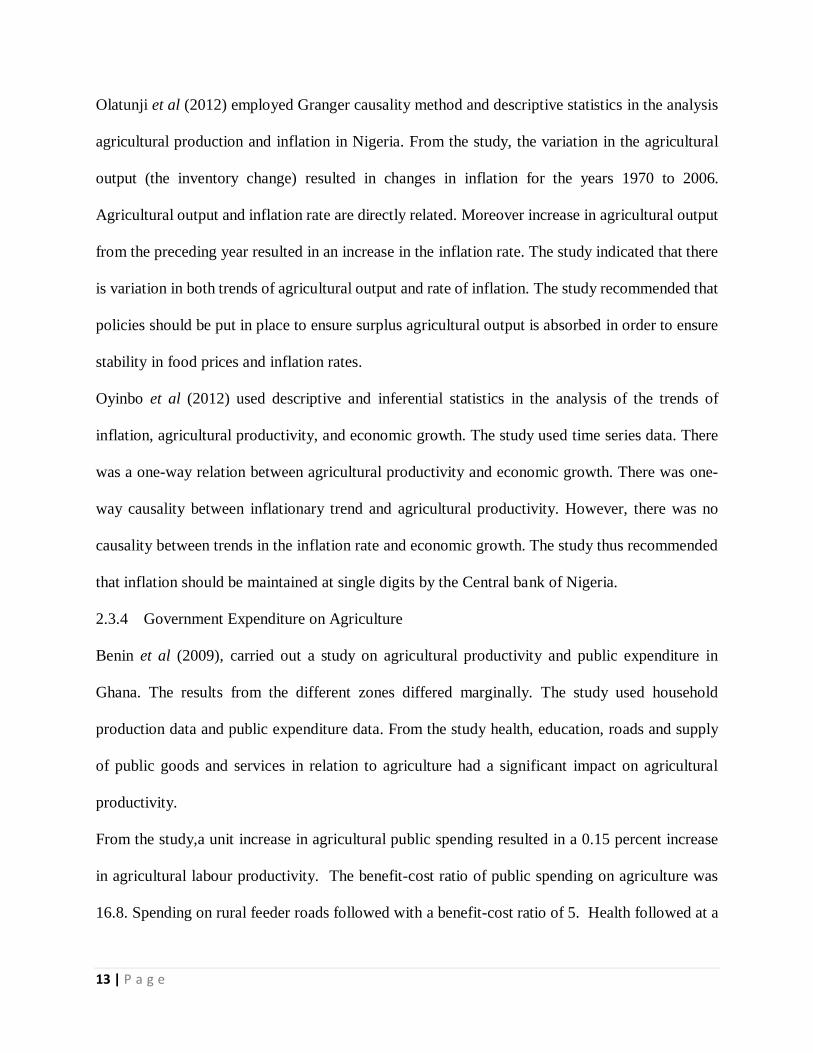
Olatunji et al (2012) employed Granger causality method and descriptive statistics in the analysis

agricultural production and inflation in Nigeria. From the study, the variation in the agricultural

output (the inventory change) resulted in changes in inflation for the years 1970 to 2006.

Agricultural output and inflation rate are directly related. Moreover increase in agricultural output

from the preceding year resulted in an increase in the inflation rate. The study indicated that there

is variation in both trends of agricultural output and rate of inflation. The study recommended that

policies should be put in place to ensure surplus agricultural output is absorbed in order to ensure

stability in food prices and inflation rates.

Oyinbo et al (2012) used descriptive and inferential statistics in the analysis of the trends of

inflation, agricultural productivity, and economic growth. The study used time series data. There

was a one-way relation between agricultural productivity and economic growth. There was one-

way causality between inflationary trend and agricultural productivity. However, there was no

causality between trends in the inflation rate and economic growth. The study thus recommended

that inflation should be maintained at single digits by the Central bank of Nigeria.

2.3.4 Government Expenditure on Agriculture

Benin et al (2009), carried out a study on agricultural productivity and public expenditure in

Ghana. The results from the different zones differed marginally. The study used household

production data and public expenditure data. From the study health, education, roads and supply

of public goods and services in relation to agriculture had a significant impact on agricultural

productivity.

From the study,a unit increase in agricultural public spending resulted in a 0.15 percent increase

in agricultural labour productivity. The benefit-cost ratio of public spending on agriculture was

16.8. Spending on rural feeder roads followed with a benefit-cost ratio of 5. Health followed at a

14 | P a g e

distant third. However, formal education had a negative effect on agricultural productivity. This

could be connected to more skilled labour which is associated with more educated people, being

allocated away from farms.

Selvaraj (1993), analyzed how variation in government expenditure affected growth in agriculture

sector in India. Agricultural development had relied significantly on financing by the government

for a long time. Over the years, the share of agriculture spending out of the public finance has been

declining. This can be attributed to the economic reforms, milestones achieved in agriculture, as

well as industrialization. This trend, however, affects the performance of agricultural sector

negatively. The study used time-series data. The results of the study clearly demonstrated the

importance of government expenditure on agriculture. Reduction in the portion allocated to

agriculture has adverse effects on performance of the agricultural sector. There was an inverse

relationship between fluctuation in government expenditure in agriculture and agricultural sector

growth.

Mutuku (1993), studied the impact of government expenditure and the structural adjustment

programmes on the agricultural sector. He noted that agricultural output can be increased through

land use intensification which includes the use of hybrid crops, farm machinery, use of fertilizers

to improve soil productivity as well as improved animal husbandry practices. He also noted that

small-scale farmers account for a significant percentage of the total agricultural output. The

infrastructure needed to raise agricultural productivity is a public good provided by the government

via government expenditure. Adequate government expenditure to the agricultural sector would

fast track agricultural development. The study found that instability in government expenditure

adversely affects agricultural sector performance. Government expenditure is important in

improving agricultural sector performance.

15 | P a g e

2.3.5 Climate/rainfall

Ayinde et al (2011), carried out a study in Nigeria on how changes in climate affected agricultural

productivity. The study used descriptive and co-integration model approach to analyze time series

data. The study concluded that during the period from 1981 to 1995, there was a steady and high

rate of agricultural productivity. However, during the period from 1996 to 2000, the rate was very

low. It was observed that the amount of rainfall and temperature had fluctuated in the later period.

Agricultural productivity and annual rainfall results from Augmented Dickey-Fuller unit root test

were not stationary but became stationary after the first differencing. Temperature (annual),

however, was stationary at its level. Temperature change was negatively related to agricultural

productivity. However, rainfall change was positively related to agricultural productivity. The

study also revealed that previous year’s rainfall had a negative effect on the productivity of the

current year. The study thus recommended that to increase and sustain agricultural productivity

there was a need to encourage innovations and technologies that are environmentally sensitive so

as to mitigate fluctuations in the climatic conditions.

Kumar & Sharma (2013), used an econometric model and the regression analysis which revealed

that extreme climate variation adversely affects the quantity and value of production for majority

of the crops. This indicates that food security is greatly threatened for most of the small scale

farming households. This is because agricultural productivity and food security are interrelated.

The study also generated food security index which revealed that it was also adversely affected by

the climatic fluctuations.

Edame et al (2011), noted adverse climate change is a major threat to food security in the 21st

century. Agriculture is very sensitive to climate change. Since the world population is growing

16 | P a g e

agricultural production should also increase to ensure food security. To successfully boost food

security, agricultural productivity needs to be boosted.

2.4 Overview of literature

From the above literature, some studies have employed Cobb-Douglas production function with

agricultural output as the dependent variables while the independent variables varied in different

studies. This study employed the Cobb-Douglas production function with the independent

variables being: labour force, climate/rainfall, real exchange rate, government expenditure and

inflation.

Research in the agricultural sector has and continues to be carried out. This can be attributed to the

significant role agricultural sector plays in the economy, especially in the developing economies.

Since agricultural sector continues to be a very significant sector of the Kenyan economy, there is

need for vigorous and extensive research so as to provide updated data to enable the relevant

authorities to formulate policies and programmes which are up to date and relevant to the current

trends.

This study will, therefore, serve the purpose of expanding the body of literature available to enable

policy makers to formulate relevant policies.

2.5 Research gaps

Further research needs to be done on individual determinants of agricultural productivity so as to

have an in-depth understanding of the contribution of individual factors without aggregating

them in a study.

17 | P a g e

CHAPTER 3

3.0 METHODOLOGY

3.1 Research design

This study applied quantitative research design where empirical data was analyzed.

Cobb-Douglas production function was estimated by ordinary least squares (OLS) to evaluate the

determinants of agricultural productivity in Kenya. Generally, productivity encompasses varied

likely combinations of measures of inputs and output. The widely used productivity measure,

combines value added which is used as a metric for output, with a proxy for labour input, which

is applied to the entire economy. This gives value added per worker, which is a partial measure of

productivity because it only considers on input ie labour input. This however is preferred as it

allows comparisons across different countries and sectors.

3.2 Conceptual framework

Independent Variables Dependent variable

Labour force

Climate/ Rainfall

Real exchange rate

Government Expenditure

Inflation

Agricultural

Productivity

18 | P a g e

Agricultural productivity(Y) was regressed against; labour force (L), rainfall(R), real exchange

rate(E), government expenditure on agriculture(G) and inflation(I).

LnYt = β0+ β 1(lnLt) + β 2(lnRt) + β 4(lnEt) + β 3(lnGt) + β 5(lnIt ) + µt

Where

Yt is agricultural productivity measured as agriculture value added per worker

Lt is labour force measured in terms of population growth rate at time t

Rt in the rainfall measured in terms of annual rainfall in Kenya at time t

Et is the real exchange rate measured as real effective exchange rate at time t

Gt is the government expenditure on agriculture at time t

It is the inflation rate measured using annual consumer price index at time t

µt is the random error term.

Definition of variables

Labour Force (L)

The labour force is proxied by total population growth rate. The relationship between labour force

and agricultural productivity is expected to be negative. This is due to the pressure on the

agricultural land with an increase in population.

19 | P a g e

Inflation (I)

Inflation is the sustained general increase in price levels of goods and services. Inflation is

measured in terms of consumer price index over time. When we consider the prices of outputs, the

relationship between price level and agricultural productivity is expected to be positive. When

inputs are considered the relationship between price levels and agricultural productivity is

expected to be negative.

Rainfall (RF)

Rainfall is a variable indexed by total annual rainfall in different counties in Kenya. It is used to

represent climate as a determinant of agricultural productivity. From theory, a positive relationship

is expected between rainfall and agricultural productivity.

Real exchange rate (E)

The real exchange rate is the purchasing power of a currency relative to another currency. In this

project, it is used as a policy variable to bring in the effect of a country’s macroeconomic and trade

policies. The real exchange rate is a macro price and affects both the prices of imported inputs and

tradeable outputs. The relationship between exchange rate and agricultural productivity is rather

uncertain.

Government expenditure in agriculture (G)

This is used to represent government direct involvement in agriculture. From theory, we expect a

positive relationship between government expenditure on agriculture and agricultural productivity.

This is attributed to increased investment by the government in the agricultural sector from input

20 | P a g e

subsidies, extension services, provision of infrastructure and research which all contribute

positively to enhancing agricultural productivity.

Agricultural productivity (Y)

Agricultural productivity proxied by agriculture value added per worker is a measure of

agricultural productivity. Value added in the agricultural sector is considered as measures the

output of the agricultural sector less the value of intermediate inputs. Agriculture comprises value

added from forestry, hunting, and fishing as well as cultivation of crops and livestock production.

This is the dependent variable in the model.

3.3 Data sources

The study utilized annual time series data for the period from 1980 to 2013. The data in this study

was obtained from various sources: The Kenya National Bureau of Statistics (KNBS); statistical

abstracts and economic surveys, and from the World Bank development indicators.

3.4 Data processing and Analysis

The study used the ordinary least squares method of estimation to estimate the parameters of the

model. To test the statistical significant of the parameters t-test was used, by comparing the t-test

critical estimates and t-test estimated values.



among the study variables.

Dickey–Fuller test for unit root was used to test for stationarity. Non-stationarity is solved through

first differencing.

21 | P a g e

CHAPTER 4

4.0 DATA ANALYSIS, FINDINGS, AND DISCUSSION

4.1 Method of Analysis

This study employed the ordinary least square estimation method to estimate the parameters of the

model. To test the statistical significance of the parameters the study employed t-test. T-critical

value (from t distribution table) and t-statistic were compared at 5% level of significance. When

the magnitude of t-statistics is great the more reliable the value of the coefficients are to predict

the dependent variable. When the magnitude of the t-statistics are close to zero the less reliable the

value of the coefficients are to predict the dependent variable.

R-squared which is the coefficient of multiple determination and F statistics were employed to

determine the overall significance of the regression equation. R-squared is a statistical measure of

how close the data are to the fitted regression line. It explains the extent to which the independent

variables affect the total variation in the dependent variable. The higher the R-squared, the better

the model fits the data.

To show the overall significance of the model specified, we used the F – test. The F statistic is

defined as (explained variation k /unexplained variation k – 1). If the F-statistic is greater than the

F critical value, then we conclude that the overall model is statistically significant or otherwise

(Shim et al., 1995). To establish whether the model is acceptable or otherwise we compared the

value of the Durbin-Watson (DW) Statistic from the multiple regression results with the value of

the R-squared. If the value of the DW statistics is greater than the value of the R-squared, then our

model is not spurious and can be accepted or otherwise (Gujarati et al, 2009).

We tested for autocorrelation which is detected by using the Durbin-Watson statistic. If the value

of the DW statistics lies between 1.5 to 2.5, this indicates that there is no problem of autocorrelation

22 | P a g e

(Shim et al, 1995). Heteroscedasticity in our specified model which is detected by using the Park

test. According to the Park test, if a statistically significant relationship exists between the log of

the error term and the explanatory variable, then, the null hypothesis (H0: no heteroscedasticity)

can be rejected.

Source of Data

Data was collected from the World Development Indicators 2014 and statistical abstracts and

economic surveys from KNBS.

Econometric Package

The econometric software used in this study was Stata.

4.2 Empirical Findings

Presentation of the results

Test for the Presence of Autocorrelation Using DW Test

Hypotheses: Null hypothesis H0: no autocorrelation. Alternative hypothesis H1: autocorrelation

DW test statistic: DW = 1.8309091

Decision rule

According to (Shim & Siegel, 1995), if the DW test statistics fall between 1.5 and 2.5 there is no

autocorrelation. If it falls below 1.5 there is positive autocorrelation. If it falls above 2.5 there is

negative autocorrelation.

DW Statistic Conclusion

Since the DW test statistic figure of 1.8309091 falls between 1.5 and 2.5 then there is no

autocorrelation.

23 | P a g e

Test for stationarity

Table 4. 1 Dickey-Fuller test for unit root

Test Statistic 1% Critical

Value

5% Critical

Value

10% Critical

Value

Z(t) – E -2.828 -2.453 -1.696 -1.309

Z(t) – I -4.225 -2.453 -1.696 -1.309

Z(t) – R -5.772 -2.453 -1.696 -1.309

Z(t) – Y -1.804 -2.453 -1.696 -1.309

Z(t) – L -1.707 -2.453 -1.696 -1.309

Z(t) – G 0.128 -2.453 -1.696 -1.309

Z(t) - G - Lag (1) -5.073 -3.702 -2.980 -2.622

From the results above we can conclude that exchange rate (E), inflation rate (I), rainfall (R) are

stationary at all levels of significance. Whereas labour force given by population growth rate (L)

is stationary at 5% and 10% level of significance. Government expenditure (G) was only stationary

at all levels of significance after lagging once. Thus we can conclude that the model is a stable

predictor of the independent variable at 5% level of significance.

Test for the Presence of Heteroscedasticity

According to (Koutsoyiannis, 2006), effects of heteroscedasticity is greatly lessened by

transforming the data into logs. All the variables in the model were consequently transformed into

logs.

Test for cointegration

Table 4. 2 Cointegration Rank for determinants of agricultural productivity, (1980-2013)

24 | P a g e

Sample: 1980 – 2013

Test assumption: linear deterministic trend in data

Series Y, E, I, L, R, GE Lags 2

Eigenvalue Likelihood

Ratio (Trace statistics)

5%

Critical Value

0.93144 134.0323 68.52

0.82152 80.6100 47.21

0.73523 39.4140 29.68

0.57533 12.8645 15.41

0.27513 2.8898 3.76

Normalized Cointegrating Coefficients: 1 cointegrating Equation

Y E I L R GE Constant

1 -

.0866485

-

.1143693

.0560059 .3787262 .0985152 -4.221326

The eigenvalues are presented in the first column, while the likelihood ratio gives the trace statistic

are presented in the second column:

The analysis is restricted to one cointegrating equation,

From Table (4.2) it can be seen that likelihood ratio test implies the choice of r=1 that is we have

one cointegrating relation. We can interpret this cointegration vector based on economic theory as

the agriculture productivity determinants.

Under the assumption of r=1 cointegrating relationship, we have one normalized Y cointegrating

equation.

25 | P a g e

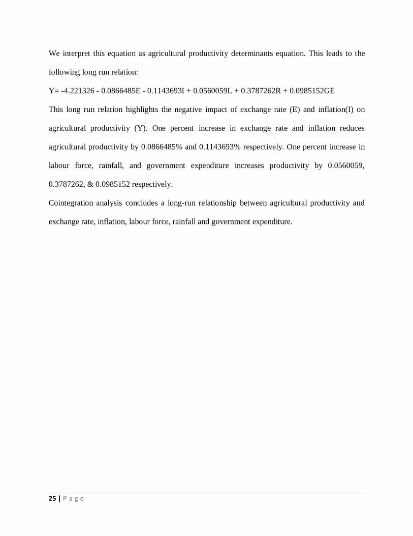
We interpret this equation as agricultural productivity determinants equation. This leads to the

following long run relation:

Y= -4.221326 - 0.0866485E - 0.1143693I + 0.0560059L + 0.3787262R + 0.0985152GE

This long run relation highlights the negative impact of exchange rate (E) and inflation(I) on

agricultural productivity (Y). One percent increase in exchange rate and inflation reduces

agricultural productivity by 0.0866485% and 0.1143693% respectively. One percent increase in

labour force, rainfall, and government expenditure increases productivity by 0.0560059,

0.3787262, & 0.0985152 respectively.

Cointegration analysis concludes a long-run relationship between agricultural productivity and

exchange rate, inflation, labour force, rainfall and government expenditure.

26 | P a g e

Table 4. 3 Error Correction Model Equations (ECM)

For the Variables, Y, E, I, L, R & GE Estimated by OLS based on Cointegrating

Regressors Y E I L R GE

ce1

L1 -.125832

(.1339856)

-.1887736

(.3945599)

8.313998

(2.016857)

.018942

(.0237973)

1.477493

(.478928)

1.446446

(.9542383)

Dlog_Y -.1328605

(.2385087)

-.447267

(.7023588)

-6.175272

(3.590221)

.0233853

(.0423617)

-.2633606

(.8525431)

-.4661141

(1.698646)

Dlog_E -.0939236

(.0843108)

-.0214892

(.2482779)

1.354942

(1.269113)

-.0150012

(.0149745)

.5009989

(.3013668)

.2410367

(.6004571)

Dlog_I -.01209

(.0115335)

-.0072875

(.0339637)

.0243545

(.1736107)

.0024236

(.0020485)

.1383145

(.041226)

.1928541

(.0821407)

Dlog_L .4395862

(.5042627)

-.5597813

(1.48495)

-15.77305

(7.590561)

.8384065

(.0895625)

-3.595226

(1.802474)

-4.612638

(3.591333)

Dlog_R -.00474

(.0561423)

-.082685

(.1653275)

1.010865

(.8450984)

.0007271

(.0099715)

-.13592

(.2006792)

.1259666

(.3998426)

Dlog_GE .0106732

(.0312009)

-.0652335

(.0918802)

-.8052844

(.4696605)

-.0035869

(.0055416)

.0588106

(.1115268)

-.4606834

(.2222111)

C .0024814

(.0104631)

.0537807

(.0308117)

.0044054

(.15749890

.0000209

(.0018584)

-.0176118

(.0374001)

-.0000966

(.0745177)

R2 0.1480 0.3231 0.3204 0.9105 0.7181 0.6613

Equation 1

Y= -4.221326 -0.0866485E - 0.1143693I + 0.0560059L + 0.3787262R + 0.0985152GE

27 | P a g e

From Table 4.3 the values of Standard errors are in brackets.

From the results of Error Correction model, labour, rainfall and government expenditure have a



respectively. This imply’s that in the short run Labour, rainfall, and government expenditure are


Table 4. 4 OLS estimates 1980-2013

Variable Coefficient Standard error t-statistics t-critical

log_E -.0405422 .0430437 -3.94

log_I -.0193286 .0139671 -2.38

log_L .1984402 .2132522 1.93 2.052

log_R .0917103 .0683248 2.34

fdlog_GE .0639032 .0402303 2.59

Const 6.021043 .5973901 10.08

Unadjusted R2 = 0.7658; Adjusted R2 = 0.7039; F-statistic F( 5, 27) =10.76 ] (p-value < 0.00001);

Dwcfdurbin-Watson statistic = 1.8309091

Using the 33 observations

Dependent variable: log_Y (Agricultural Productivity)

4.3 Discussion of results

The value of DW statistics (1.8309091) is greater than that of R-squared (0.7658) thus the

regression result is not spurious. This model for agricultural productivity in Kenya can, therefore,

be accepted and meaningful conclusions drawn based on the results. Statistically, the model is a

28 | P a g e

good fit as the values of unadjusted R-squared is 0.7658. This implies that 76.58% of total variation

in agricultural productivity in Kenya can be explained by the inflation rate, government

expenditure on agriculture, exchange rate, labour force and climate (rainfall). Overall the model is

statistically significant as the value of F-statistics (10.76) is greater than the f-critical value

(2.07298) at one percent level of significance.

From the above tests, it could be seen that regression results are not affected by the problems of

autocorrelation, non-stationarity, and heteroscedasticity.

From the regression results, a one percent increase in exchange rate will cause a 0.405422%

decrease in agricultural productivity. From literature the relationship between exchange rate and

agricultural productivity is uncertain. Exchange rate affects both the prices of imported inputs and

tradeable outputs. In this case, we can conclude the impact of exchange rate on imported inputs

outweighed the effect on agricultural outputs. An increase in exchange rate affect inputs which are

imported negatively which consequently adversely affects productivity. Thus an increase in

exchange rate resulted in a decrease in productivity. The findings contradict those of (Brownson

et al, 2012).

A one percent increase in annual rainfall resulted in an increase of 0.0917103% in agricultural

productivity. This is due to the fact that agriculture in Kenya is still largely dependent on rain-fed

agriculture, despite the government effort in investing in irrigation schemes as only a small percent

of land is under irrigation. This is within expectation as an increase in rainfall was hypothesized

to cause an increase in agricultural productivity. It is consistent with the findings of (Ayinde et al,

2011).

A one percent increase in government expenditure on agriculture resulted in an increase in

agricultural productivity by 0.0639032%. From theory Government investment in the agricultural

29 | P a g e

sector is critical in boosting agricultural productivity. Thus the results of the regression results

conform to expectations. This finding is consistent with (Benin et al, 2009) and (Selvaraj, 1993).

A one percent increase in annual inflation rate results in a decrease in agricultural productivity by

0.0193286%. We hypothesized that there will be a positive relationship between inflation and

agricultural productivity in Kenya. However, a negative relationship was realized. This can be

explained by the fact that inflation affects the price levels of both output and inputs. Thus if the

price level of inputs is too high this will impact agricultural productivity negatively. This finding

is consistent with (Brownson et al, 2012).

A one percent increase in labour force causes an increase in agricultural productivity by

0.1984402%. This can be attributed to the fact that agricultural sector in a significant source of

employment in Kenya thus increase in labour force will result in an increase in agricultural

productivity. This finding is consistent with (Abugamea, 2008), (Odhiambo et el, 2004) and

(Ekborn, 1998).

30 | P a g e

CHAPTER 5

5.0 SUMMARY, CONCLUSION AND RECOMMENDATIONS

5.1 Summary

This study set out to examine the factors that influence agricultural productivity in Kenya. This

study applied quantitative research design to analyze empirical data. The main objective of the

study was to establish the factors which influence agricultural productivity in Kenya. The Cobb-

Douglas production function and Ordinary Least Square estimation technique were employed as

the method of estimation. The dependent variable in the model is Agricultural productivity while

the independent variables were inflation rate, exchange rate, government expenditure, climate

(rainfall), and labour force. Apart from labour force, all other independent variables in the model;

inflation rate, exchange rate, government expenditure, climate (rainfall) are statistically

significant. The study utilized annual time series data from 1980 to 2013.



among the study variables. The long run relation highlights the negative impact of the exchange

rate (E) and inflation (I) on agricultural productivity (Y), while Labour force, rainfall, and

government expenditure impact agricultural productivity positively. In the short run Labour,

rainfall, and government expenditure are the main determinants of agricultural productivity in

Kenya.

31 | P a g e

5.2 Conclusion

From the regression results, one percent increase in agricultural expenditure caused an increase of

0.0639032%. One percent increase in annual rainfall caused an increase of 0.0917103% in

agricultural productivity. One percent increase in labour force caused an increase of 0.1984402%

in agricultural productivity. One percent increase in inflation rate caused a 0.0193286% decrease

in agricultural productivity. Finally, one percent increase in exchange rate caused 0.405422%

decrease in agricultural productivity.

From the results of Error Correction Model, labour, rainfall and government expenditure have a



respectively. This implies that in the short run Labour, rainfall, and government expenditure are


This long-run relation highlights the negative impact of exchange rate (E) and inflation (I) and

agricultural productivity (Y). One percent increase in exchange rate and inflation reduces

agricultural productivity by 0.0866485% and 0.1143693% respectively. One percent increase in

Labour force, rainfall, and government expenditure increases productivity by 0.0560059,

0.3787262, & 0.0985152 respectively. Cointegration analysis concludes a long-run relationship

between agricultural productivity and exchange rate, inflation, labour force, rainfall and

government expenditure.

Productivity is a critical attribute in the agricultural sector. Improvement in productivity will foster

food security, increase foreign exchange inflow as well as contribute to poverty reduction

especially in the rural areas.

32 | P a g e

5.3 Policy Recommendations

From the findings of the study, the following policy recommendations are suggested:

1. The government should continually ensure inflation rates are maintained at single digits both in

the short-run and long-run.

2. Efforts should continually be made to expand and modernize existing irrigation schemes and

establish new ones to ensure the country is not too reliant on rain-fed agriculture.

3. The government should continue to invest in agriculture through budgetary allocation to the

sector as agriculture is still a very significant sector in Kenya’s Economy.

5.4 Areas of further study

This study combined the effect of five factors and their effect on agricultural productivity in

Kenya. Further research needs to be done on individual determinants of agricultural productivity

so as to have an in-depth understanding of the contribution of individual factors without

aggregating them in a study.

33 | P a g e

REFERENCES

Abugamea, H. (2008). A Dynamic Analysis for Agricultural production Determinants in

Palestine : 1980 - 2003. Conference on Applied Economics - ICOAE 2008.

Ahmad, K. (2012). Determinants of Agriculture Productivity Growth in Pakistan. International

Research Journal of Finance and Economics, 1450-2887(95), 164-172.

Anyanwu, S. (2013). Determinants of Aggregate Agricultural productivity among high external

inputs technology farms in a harsh macroeconomic environment of IMO state, Nigeria.

African Journal of Food, Agriculture, Nutrition and Development, 13(5), 8238-8248.

Ayinde, O., Muchie, M., & Olatunji, G. (2011). Effect of Climate Change on Agricultural

Productivity in Nigeria. Journal ofHuman Ecology, 35(3), 189-194.

Benin, S., Mogues, T., Cudjoe, G., & Randriamamonjy, J. (2009). Public Expenditure and

Agricultural Productivity Growth in Ghana. Beijing: International Food Policy Research

Institute.

Brownson, S., Vincent, I.-M., Emmanuel, G., & Etim, D. (2012). Agricultural Productivity and

Macro-Economic Variable Fluctuation. International Journal of Economics and

Finance;, 4(8), 114-125.

Brownson, S., Vincent, I.-m., Emmanuel, G., & Etim, D. (2012). Agricultural Productivity and

Macro-Economic Variable Fluctuation in Nigeria. International Journal of Economics

and Finance; 4(8), 114-125.

Edame, G., Ekpenyong, A., Fonta, W., & EJC, D. (2011). Climate Change, Food Security and

Agricultural Productivity in Africa: Issues and Policy Directions. International Journal of

Humanities and Social Science, 1(21), 205-223.

Ekborn, A. (1998). Some Determinants of Agricultural Productivity - an Application of Kenyan

Highlands. Washington D.C. 20433 U.S.A: World Bank, African Region, Environmental

group (J3-141), 1818H St.

Enu, P., & Attah-Obeng, P. (2013). Which Macro Factors Influence Agricultural Production in

Ghana. Academic Research International, 4(5), 333-346.

Government of Kenya. (2007). Kenya Vision 2030. Nairobi, Kenya: Government press.

Government of Kenya. (2010). Agricultural Sector Development Strategy. Nairobi: Government

of Kenya.

Gujarati, D. N., & Porter, D. C. (2009). Basic Econometrics). Basic Econometrics . Singapore:

McGraw– Hill.

KNBS. (2015). Economic Survey. Nairobi: Kenya National Bureau of Statistics.

Koutsoyiannis, A. (2006). Theory of Econometrics: An introductory Exposition of Econometric

Methods (2nd ed.). India,: Barners & Noble Books.

34 | P a g e

Kumar , A., & Sharma, P. (2013). Impact of Climate Variation on Agricultural. Economics E-

Journals, 2013-43.

Mutuku, K. (1993). Government.expenditure, structural adjustment and the performance of

agricultural sector in Kenya. Nairobi.

Odhiambo, W., Nyangito, H. O., & Nzuma, J. (2004). Sources and Determinants of Agricultural

growth and productivity in Kenya. Nairobi, Kenya: Kenya Institute for Public Policy

Research and Analysis(KIPPRA), Discussion paper No. 34.

Olatunji, G., Omotesho, O., Ayinde, O., & Adewumi, M. (2012). Empirical Analysis of

Agricultural Production and Inflation Rate in Nigeria. African Journals Online, 12(1), 21-

30.

Oyinbo, O., Owolabi, J., Hassan, O., & Rekwot, G. (2012). Inflationary trend, Agricultural

productivity and economic growth in nigeria: The links. Sokoto Journal of the Social

Sciences, 2(1), 1-11.

Selvaraj, K. (1993). Impact of Government Expenditure on Agriculture and Performance of

Agricultural Sector in India. Bangladesh Journal of Agricultural Economics, 16(2), 37-

49.

Shim, J. K., & Siegel, J. G. (1995). Dictionary of Economics. USA: John Wiley and Sons, Inc.

World Bank. (2011). The Need to Boost Agricultural Productivity. In W. Bank, Growth and

Productivity in Agriculture and Agribusiness (978-0-8213-8606-4), 1-10.

World Bank Group. (2015). World Bank Group. Retrieved September 10/09/2015, 2015, from

www.worldbank.org

Documents

Determinants of Agricultural Productivity in Kenya