Determinants, Areas and Volumes

Theodore Voronov

December 4, 2005

The aim of these notes is to relate the algebraic notion of determinantwith the geometric notions of area and volume (and their multidimensionalgeneralizations) in order to make it possible to use these concepts in furthergeometry and calculus/analysis courses.

Contents

1 Determinants 21.1 Matrices and vectors . . . . . . . . . . . . . . . . . . . . . . . 21.2 Determinant as a multilinear alternating function . . . . . . . 41.3 Properties of determinants . . . . . . . . . . . . . . . . . . . . 71.4 Calculations . . . . . . . . . . . . . . . . . . . . . . . . . . . . 101.5 Problems . . . . . . . . . . . . . . . . . . . . . . . . . . . . . . 14

2 Areas and Volumes 172.1 Why the area of a parallelogram is represented by a determinant 172.2 Volumes and determinants . . . . . . . . . . . . . . . . . . . . 212.3 Areas and volumes in Euclidean space . . . . . . . . . . . . . 222.4 Examples and applications . . . . . . . . . . . . . . . . . . . . 25

2.4.1 The distance between a point and a plane . . . . . . . 262.4.2 Area of a piece of the plane or a surface . . . . . . . . 27

2.5 Problems . . . . . . . . . . . . . . . . . . . . . . . . . . . . . . 29

1

§1 Determinants

You might have met determinants of small order (two by two and three bythree) in high school algebra and you will definitely study determinants indetail in the linear algebra course. Here we shall remind the definition andbasic facts about determinants in the form most convenient for seeing theirgeometric meaning.

1.1 Matrices and vectors

We shall consider a set denoted Rn. By definition, its elements are arrays ofreal numbers of length n:

Rn = {x = (x1, . . . , xn) | xi ∈ R for all i = 1, . . . , n} .

We shall call elements of Rn, vectors. The set Rn is called the n-dimensionalarithmetic space. For a given vector x the numbers xi are called its coor-dinates or components. Vectors can be added and multiplied by numberscomponentwise:

Example 1.1. (−2, 5, 1, 0) + (0, 1, 7,−1) = (−2, 6, 8,−1),3(−2, 5, 1, 0) = (−6, 15, 3, 0)

Clearly, we can add vectors only of the same size, i.e., for a fixed n. Lateron you will study the general notion of a ‘vector space’ of dimension n andwill learn that Rn is the first example of such a space.

Vectors in Rn can be written as rows: x = (x1, . . . , xn), or as columns:

x =

x1

. . .xn

.

If we need to make a distinction, then we refer to these two ways of represent-ing vectors as to row-vectors or column-vectors. One can consider rectangulararrays of more general kind, with n rows and m columns:

A =

a11 a12 . . . a1m

a21 a22 . . . a2m

. . . . . . . . . . . .an1 an2 . . . anm

2

Such arrays are called matrices or n × m matrices when it is necessary toindicate the dimensions. The numbers ij in the notation aij serve as labelsspecifying the element in the ith row and jth column. They are pronounced,for example “two, three” for a23, not “twenty three”. The elements of amatrix are also called matrix entries. Row-vectors and column-vectors areparticular cases of matrices (with only one row or only one columns, respec-tively). An important role is played by matrices with n = m, called squarematrices.

Example 1.2. A =

(2 0−1 8

)is a 2 × 2 matrix (a square matrix). Here

a11 = 2, a12 = 0, a21 = −1, a22 = 8.

Example 1.3. There are two special matrices. The zero matrix

0 =

0 . . . 0. . . . . . . . .0 . . . 0

(all entries are zeros) is defined for any n and m. In particular, there isthe zero vector in Rn, all coordinates of which are zero. When n = m, i.e.,among square matrices, there is another important matrix called the identitymatrix :

E =

1 0 . . . 00 1 . . . 0

. . . . . . . . . . . .0 0 . . . 1

.

Its entries on the diagonal are 1 and all others are 0. An alternative notationis I. If we need to stress the dimension, the we can write En or In.

In the same way as for vectors, matrices of a fixed size can be multipliedby numbers and added or subtracted. This is done entry by entry:(

1 3 0−2 0 5

)+

(0 2 11 4 −2

)=

(1 5 1−1 4 3

)

7

(2 2−3 0

)=

(14 14−21 0

)

A non-trivial operation in the matrix algebra is the matrix multipli-cation. It is introduced as follows. First we define the product of a row-

vector a = (a1, . . . , an) with a column-vector b =

b1

. . .bn

as the number

3

ab = a1b1 + · · · + anbn. This extends to more general matrices. If we aregiven a matric A with n rows and p columns, and a matrix B with p rowsand m columns, then each row of A can be multiplied with each column ofB according to the above rule, giving, by the definition, a matrix element ofthe matrix product of A and B:

A =

a11 a12 . . . a1p

. . . . . . . . . . . .an1 an2 . . . anp

, B =

b11 . . . b1m

b21 . . . b2m

. . . . . . . . .bp1 . . . bpm

,

AB =

a11b11 + a12b21 + · · ·+ a1pbp1 . . . a11b1m + a12b2m + · · ·+ a1pbpm

. . . . . . . . .an1b11 + an2b21 + · · ·+ anpbp1 . . . an1b1m + an2b2m + · · ·+ anpbpm

.

In other words, we take the products of the first row of A with all the columnsof B and thus obtain the first row of AB; then take the products of the secondrow of A with the columns of B to obtain the second row of AB, and so on.The product of an n×p matrix with a p×m matrix will be an n×m matrix.This contains the product of a row-vector and a column-vector, giving anumber (a ‘1× 1 matrix’), as a particular case.

The matrix multiplication is associative, i.e., satisfies A(BC) = (AB)C,and distributive w.r.t. the addition of matrices. However, in general it is nottrue that AB equals BA even if the dimensions are matching. One can checkthat A0 = 0A = 0 and AE = EA = A for all matrices A.

1.2 Determinant as a multilinear alternating function

The determinant det A is a particular polynomial function of the matrixentries of a square matrix A. It has the appearance of the sum of productsof elements each belonging to a different row of the matrix A (and also to adifferent column) taken with certain signs.

Example 1.4. For a 1 × 1 matrix, which is just a number, A = a, thedeterminant coincides with this number: det A = a.

Example 1.5. For a 2× 2 matrix A =

(a bc d

)we have

det A = ad− bc

(you can memorize this formula).

4

Example 1.6. For a 3× 3 matrix A =

a11 a12 a13

a21 a22 a23

a31 a32 a33

we have

det A = a11a22a33− a11a23a32− a12a21a33− a13a22a31 + a13a21a32 + a12a23a31 .

(you do not have to memorize this formula).

Determinants appear in innumerable applications and are, without exag-geration, the most important algebraic notion.

The easiest way to actually define the determinant, so that it will be clearhow to calculate it for a particular matrix and to see which properties doesit have in general, is to do so by using the axiomatic method.

Consider a square n× n matrix A as consisting of n column-vectors (wetreat each column of A as a vector). So we can write A = (a1, . . . , an) whereai stands for the ith column of A.

Theorem 1.1. There is exists a unique polynomial function D(A) of thematrix entries of A such that when considered as a function D(a1, . . . , an) ofthe columns a1, . . . , an it has the following properties:

(1) if any column is multiplied by a number, it can be taken out:

D(a1, . . . , cak, . . . , an) = cD(a1, . . . , ak, . . . , an)

(for all k = 1, 2, . . . , n);(2) if any column is substituted by the sum of two arbitrary column-

vectors, the function will become the sum:

D(a1, . . . , a′ + a′′︸ ︷︷ ︸

kth place

, . . . , an) = D(a1, . . . , a′, . . . , an) + D(a1, . . . , a

′′, . . . , an)

(for all k = 1, 2, . . . , n);(3) it any two columns are swapped, then the function changes sign:

D(a1, a2, a3, . . . , an) = −D(a2, a1, a3, . . . , an)

(and the same for any pair of columns ai and aj, where i, j = 1, . . . , n);(4) for the identity matrix, D(E) = 1.

5

Proof. We shall give a proof for the case n = 2, and it will be clear how thesame logic works for an arbitrary n. Assume that the properties (1) to (4)hold for a function D(A). As we shall see, this will allow to obtain a uniqueformula for D(A). (This establishes the uniqueness part of the theorem.)Taking it as the definition of D(A), we shall notice that the properties willbe indeed satisfied. (This establishes the existence part.) So consider a 2× 2matrix A. Assuming the existence of D(A) with the above properties weobtain:

D(A) = D(a1, a2) = D

(a11 a12

a21 a22

)= D

(a11e1 + a21e2, a12e1 + a22e2

)=

a11a12 D(e1, e1) + a11a22 D

(e1, e2

)+ a21a12 D

(e2, e1

)+ a21a22 D

(e2, e2

).

Here e1 =

(10

), e2 =

(01

). We used the properties (1) and (2) to “open the

brackets”. Now we shall use the property (3). (Note that it implies vanishingof D(A) if two columns of the matrix coincide.) We have, continuing thecalculation,

D(A) = a11a22 D(e1, e2

)+ a21a12 D

(e2, e1

)=

a11a22 D(e1, e2

)− a21a12 D(e1, e2

)=

(a11a22 − a21a12

)D

(e1, e2

),

where we used D(e1, e1) = D(e2, e2) = 0 and D(e1, e2) = −D(e2, e1). Fi-nally, noticing that D(e1, e2) = D(E) = 1, we arrive at the formula

D(A) = a11a22 − a21a12.

It can be immediately seen that the function defined by this explicit formulawill enjoy all the properties (1) to (4). The theorem is proved for n = 2.Similar argument works for all n.

Functions satisfying (3) are called alternating or skew-symmetric. Prop-erties (1) and (2) are referred to as linearity. ‘Multilinearity’ means linearityw.r.t. each of the arguments.

Definition 1.1. The function D(A) defined by the properties (1)–(4) ofTheorem 1.1 is called the determinant of a matrix A and denoted eitherdet A or |A| or ∣∣∣∣∣∣

a11 . . . a1n

. . . . . . . . .an1 . . . ann

∣∣∣∣∣∣

6

(we use round brackets for a matrix and vertical straight lines, for its deter-minant).

We shall shortly see how such a definition by a set of properties or ax-ioms leads to practical ways of calculating determinants. Let us make someremarks.

Remark 1.1. From the proof of Theorem 1.1 follows that an arbitrary func-tion of D(A) possessing the properties (1)–(3) but not necessarily (4), isunique up to a factor:

D(A) = det A ·D(E) .

Remark 1.2. We have already noticed that if two columns of a matrix Acoincide, then det A = 0. If for a matrix A, a column is replaced by the sumwith a multiple of another column, then the determinant will not change.(That is, if a column ai is replaced by ai + c aj, for an arbitrary j, thenthe determinant of the new matrix will be the same det A. Indeed, the newdeterminant will be the sum of det A and the one with two repeating columnsaj, at the ith and jth places, which is zero.)

Remark 1.3. The property (1) in Theorem 1.1, in fact, implies the property (2),as long as we consider polynomial functions. Indeed, a polynomial function of avector with the property f(ca) = c f(a) can only be of degree one, i.e., a linearfunction.

1.3 Properties of determinants

In this subsection we shall give the main properties of determinants. They allfollow from the fundamental properties of skew-symmetricity, multilinearityand det E = 1 that we have used for the definition of determinant. Proofscan be found at the end of the subsection.

The most important property of determinants is contained in the followingstatement.

Theorem 1.2. Determinant is a multiplicative function of a matrix: forarbitrary n× n matrices A and B,

det(AB) = det A · det B .

7

Remark 1.4. The determinant of the product is the product of determinants.You should be warned that it is not true that the determinant of the sum is thesum of determinants! In fact, there is a formula for det(A + B), but it is quitecomplicated.

We have considered determinant as a function of the matrix columns.What about the properties of det A as a function of rows?

Theorem 1.3. The determinant det A of a square matrix A is a multilinearalternating function of the rows of A. (That is, det A possesses the sameproperties (1)–(3) w.r.t. the rows as it has w.r.t. the columns. It is uniquelydefined by these conditions and the condition det E = 1.)

For an n×m matrix A with the entries aij, the transpose of A, notation:AT , is defined as the m× n matrix of the form

AT =

a11 a21 . . . an1

a12 a22 . . . an2

. . . . . . . . . . . .a1m a2m . . . anm

.

In other words, the columns of AT are the rows of A written as column-vectors, and vice versa. The (ij)-th matrix element of AT is aji, the (ji)-thelement of A.

Example 1.7. (2 3−1 0

)T

=

(2 −12 0

)

Theorem 1.4. For any square matrix A,

det AT = det A .

Determinants have several other important properties, which we shall notdiscuss here. For example, it is possible to give a closed “general formula” forthe determinant of an n×n matrix, generalizing the formulas for determinantsof orders 2 and 3 given above in Examples 1.5 and 1.6. However, it is moreimportant to develop practical methods of calculating determinants, whichis done in the next subsection.

Proofs of Theorems 1.2, 1.3 and 1.4 follow. Notice that they are all basedon the axioms (multilinearity and skew-symmetricity with respect to columns) bywhich we defined the determinant.

8

Proof of Theorem 1.2. Consider det(AB) as a function of the columns of B. De-note them b1, . . . ,bn. Notice that the columns of the matrix AB are the column-vectors Ab1, . . . , Abn (check the definition of the matrix product). It follows thatif a column of B is multiplied by a number c, the corresponding column of ABwill be multiplied by c. Similarly, if two columns of B are interchanged, then thecorresponding columns of AB will be interchanged. Therefore, by the propertiesof the determinant applied to det(AB), it follows that det(AB) as a function ofb1, . . . ,bn possesses the properties (1)–(3) of Theorem 1.1.

Proof of Theorem 1.3. Notice that for a matrix A, the multiplication from the leftby a matrix B acts as a transformation of rows of A. In particular, for

B =

c 0 . . . 00 1 . . . 0

. . . . . . . . . . . .0 0 . . . 1

the map A 7→ BA is the multiplication of the first row of A by the number c.Similarly, by putting c on the kth place on the diagonal (and keeping other diagonalelements equal to 1 and all off-diagonal, to 0) we obtain the matrix such thatA 7→ BA is the multiplication of the kth row by c. Notice that the determinant ofsuch matrix B equals c, for any k = 1, . . . , n (as it obtained from E by multiplyingthe kth column by c). Hence, by Theorem 1.2, if a row of A is multiplied by c,the determinant of the resulting matrix will be det(BA) = detB det A = c detA.This implies linearity (see Remark 1.3). In the same way we can perform theinterchange of two rows of A by multiplying A from the left by a certain matrixB. For example, A 7→ BA with

B =

0 1 0 . . . 01 0 0 . . . 00 0 1 . . . 0

. . . . . . . . . . . . . . .0 0 0 . . . 1

acts as the interchange of the first and the second rows of A. Here B is obtainedfrom the identity matrix E by swapping the first and the second column. Hencedet B = −1. For given i and j, one can similarly construct B such that A 7→ BAis the interchange of the ith row and the jth row. By Theorem 1.2 we havedet(BA) = detB detA = −det A for the result of the interchange. That meansthat detA is also an alternating function of rows, and the theorem is proved.

Proof of Theorem 1.4. Consider f(A) = detAT as a function of the columns ofA. Since the columns of A are exactly the rows of AT , and by Theorem 1.3,

9

det AT is a multilinear alternating function of the rows of AT , it follows thatf(A) = detAT is a multilinear alternating function of the columns of A. Noticealso that f(E) = detET = 1, since ET = E. Hence f(A) satisfies all the properties(1)–(4) of Theorem 1.1 and must coincide with detA.

1.4 Calculations

Example 1.8. If a matrix A has a zero row or a zero column, then det A = 0.Indeed, it follows from linearity. A linear function is zero for a zero argument:if f(c a) = c f(a), then f(0) = f(c0) = c f(0) for any c, so f(0) = 0.

Example 1.9. For a diagonal 2 × 2 matrix we have

∣∣∣∣a 00 d

∣∣∣∣ = ad − 0 = ad.

In general, for a diagonal n×n matrix, its determinant is the product of thediagonal entries: ∣∣∣∣∣∣

λ1 . . . 00 . . . 00 . . . λn

∣∣∣∣∣∣= λ1λ2 . . . λn

Indeed, λi can be taken out successively from each row (using linearity) untilwe obtain the identity matrix.

Example 1.10. If a matrix has all zeros below the diagonal, its determinantis again the product of the diagonal entries.

Consider, for example, the case n = 3. Suppose

A =

a11 a12 a13

0 a22 a23

0 0 a33

.

We have

det A = a33

∣∣∣∣∣∣

a11 a12 a13

0 a22 a23

0 0 1

∣∣∣∣∣∣= a33

∣∣∣∣∣∣

a11 a12 00 a22 00 0 1

∣∣∣∣∣∣= a33a22

∣∣∣∣∣∣

a11 a12 00 1 00 0 1

∣∣∣∣∣∣=

a33a22

∣∣∣∣∣∣

a11 0 00 1 00 0 1

∣∣∣∣∣∣= a33a22a11

∣∣∣∣∣∣

1 0 00 1 00 0 1

∣∣∣∣∣∣= a33a22a11 ,

and the claim holds. Here we repeatedly used Remark 1.2 — more precisely, itsanalog for rows: adding to any row a multiple of another row will not change thedeterminant. In the same way we can treat the case of general n.

10

The same method of ‘row operations’ (i.e., simplifying the matrix bymultiplying/dividing a row by a number and adding a multiple of one row toanother) can be effectively applied for calculating an arbitrary determinant.

Example 1.11. Calculate

∣∣∣∣∣∣

1 −2 02 0 43 −5 5

∣∣∣∣∣∣. We have

∣∣∣∣∣∣

1 −2 02 0 43 −5 5

∣∣∣∣∣∣=

∣∣∣∣∣∣

1 −2 00 4 40 1 5

∣∣∣∣∣∣= 4

∣∣∣∣∣∣

1 −2 00 1 10 1 5

∣∣∣∣∣∣= 4

∣∣∣∣∣∣

1 −2 00 1 10 0 4

∣∣∣∣∣∣= 4 · 4 = 16 .

There is another general method of calculating determinants of arbitraryorder n, known as ‘row expansion’ (or, a variant called ‘column expansion’).

Let us first consider one example.

Example 1.12. Suppose that a matrix A in a certain row has all entries equal tozero except for one equal to 1. (A variant: the same for a column.) What can besaid about its determinant? Consider a particular case of this situation. Let thefirst row of A has 1 as the first element and 0 at all other places:

A =

1 0 . . . 0a21 a22 . . . a2n

. . . . . . . . . . . .an1 an2 . . . ann

.

Then we can repeatedly apply row operations, subtracting the first row multipliedby a21, a22, etc., respectively, from the second, the third, etc., and the last row.We arrive at

detA =

∣∣∣∣∣∣∣∣

1 0 . . . 0a21 a22 . . . a2n

. . . . . . . . . . . .an1 an2 . . . ann

∣∣∣∣∣∣∣∣=

∣∣∣∣∣∣∣∣

1 0 . . . 00 a22 . . . a2n

. . . . . . . . . . . .0 an2 . . . ann

∣∣∣∣∣∣∣∣.

What is the value of the resulting determinant? Notice that is a function f(r1, . . . , rn−1)of the n − 1 row-vectors r1 = (a22, . . . , a2n), . . . , rn−1 = (an2, . . . , ann) belongingto Rn−1. Clearly, from the properties of detA follows that this function is linearin each row-vector and alternating. Hence it is the (n− 1)× (n− 1) determinant∣∣∣∣∣∣

a22 . . . a2n

. . . . . . . . .an2 . . . ann

∣∣∣∣∣∣up to a factor equal to the value of f(r1, . . . , rn−1) at the identity

11

matrix. We have

f(E) =

∣∣∣∣∣∣∣∣

1 0 . . . 00 1 . . . 0

. . . . . . . . . . . .0 0 . . . 1

∣∣∣∣∣∣∣∣= det E = 1

(here at the LHS the identity matrix E is (n− 1)× (n− 1), while at the RHS theidentity matrix is n× n). Hence, finally,

detA =

∣∣∣∣∣∣∣∣

1 0 . . . 0a21 a22 . . . a2n

. . . . . . . . . . . .an1 an2 . . . ann

∣∣∣∣∣∣∣∣=

∣∣∣∣∣∣

a22 . . . a2n

. . . . . . . . .an2 . . . ann

∣∣∣∣∣∣.

What will change if 1 appears as the second element in the first row rather thanthe first? Similarly to the above we will have∣∣∣∣∣∣∣∣∣∣

0 1 0 . . . 0a21 a22 a23 . . . a2n

a31 a32 a33 . . . a3n

. . . . . . . . . . . . . . .an1 an2 an3 . . . ann

∣∣∣∣∣∣∣∣∣∣

=

∣∣∣∣∣∣∣∣∣∣

0 1 0 . . . 0a21 0 a23 . . . a2n

a31 0 a33 . . . a3n

. . . . . . . . . . . . . . .an1 0 an3 . . . ann

∣∣∣∣∣∣∣∣∣∣

= C·

∣∣∣∣∣∣∣∣

a21 a23 . . . a2n

a31 a33 . . . a3n

. . . . . . . . . . . .an1 an3 . . . ann

∣∣∣∣∣∣∣∣,

where C is the value of the original n × n determinant when the row-vectorsr1 = (a21, a23, . . . , a2n), . . . , rn−1 = (an1, an3, . . . , ann) make the identity matrix(n− 1)× (n− 1). We have

C =

∣∣∣∣∣∣∣∣∣∣

0 1 0 . . . 01 0 0 . . . 00 0 1 . . . 0

. . . . . . . . . . . . . . .0 0 0 . . . 1

∣∣∣∣∣∣∣∣∣∣

= −1

because this is just the determinant of the n×n identity matrix with the first andsecond rows swapped (equivalently, the first and second column swapped). Hence

∣∣∣∣∣∣∣∣∣∣

0 1 0 . . . 0a21 a22 a23 . . . a2n

a31 a32 a33 . . . a3n

. . . . . . . . . . . . . . .an1 an2 an3 . . . ann

∣∣∣∣∣∣∣∣∣∣

= −

∣∣∣∣∣∣∣∣

a21 a23 . . . a2n

a31 a33 . . . a3n

. . . . . . . . . . . .an1 an3 . . . ann

∣∣∣∣∣∣∣∣.

12

One can in the same way see that for 1 at the kth position in the first row, theanswer will include the factor (−1)k−1:∣∣∣∣∣∣∣∣∣∣

0 . . . 0 1 0 . . . 0a21 . . . a2,k−1 a2k a2,k+1 . . . a2n

a31 . . . a3,k−1 a3k a3,k+1 . . . a3n

. . . . . . . . . . . . . . . . . . . . .an1 . . . an,k−1 ank an,k+1 . . . ann

∣∣∣∣∣∣∣∣∣∣

= (−1)k−1

∣∣∣∣∣∣∣∣

a21 . . . a2,k−1 a2,k+1 . . . a2n

a31 . . . a3,k−1 a3,k+1 . . . a3n

. . . . . . . . . . . . . . . . . .an1 . . . an,k−1 an,k+1 . . . ann

∣∣∣∣∣∣∣∣.

The main idea in this example is that, for matrices of a special appearance,the determinant of order n reduces to a determinant of order n − 1. This can beused for a general practical algorithm of calculating determinants.

Theorem 1.5 (“Expansion in the first row”). An arbitrary determinantof order n can be calculated via determinants of orders n− 1 as follows:

det A = a11M11 − a12M12 + · · ·+ (−1)n−1a1nM1n

where a11, . . . , a1n are the entries of the first row and M11, . . . , M1n are thedeterminants of the (n−1)×(n−1) matrices obtained from A by crossing outthe first row and the first, the second, . . . , and the last columns, respectively.

Proof. Consider the first row of A. It is the sum a11e1 + · · · + a1nen where ek,k = 1, . . . , n, is the row-vector with the single nonzero entry equal to 1 at the kthplace. By the linearity of detA, we have detA = a11 det A1+· · ·+ann det An whereAk is the n×n matrix obtained from A by replacing its first row by ek. These areexactly the determinants calculated in Example 1.12, so detAk = (−1)k−1M1k, forall k = 1, . . . , n, which proves the theorem.

The determinants M11, . . . , M1n (and similar ones) are called the minorsof the matrix A. In general, a minor of A is the determinant of the squarematrix obtained from A by crossing out some rows and columns (the samenumber of rows and columns). There are generalizations of the above ex-pansion including other minors. In particular, there is an expansion in thesecond row (instead of the first row), and in any given row, and in the firstcolumn, as well as in any given column. The formulas are similar to theabove, but the signs will depend both on a row and a column.

Example 1.13. Calculate the determinant of the 3×3 matrix

2 1 10 −3 51 0 3

13

using the expansion in the first row. Solution: we have

∣∣∣∣∣∣

2 1 10 −3 51 0 3

∣∣∣∣∣∣= 2

∣∣∣∣−3 50 3

∣∣∣∣−∣∣∣∣0 51 3

∣∣∣∣+∣∣∣∣0 −31 0

∣∣∣∣ = 2(−3·3)−(−5)+3 = −18+5+3 = −10 .

Example 1.14. Calculate the determinant of the 4×4 matrix

1 1 0 4−2 0 3 60 1 5 −13 −3 6 1

using the expansion in the first row. Solution: calculate first the minors M11, . . . ,M14. We have

M11 =

∣∣∣∣∣∣

0 3 61 5 −1−3 6 1

∣∣∣∣∣∣= −3

∣∣∣∣1 −1−3 1

∣∣∣∣ + 6∣∣∣∣

1 5−3 6

∣∣∣∣ = −3 · 4 + 6 · 21 = 114

M12 =

∣∣∣∣∣∣

−2 3 60 5 −13 6 1

∣∣∣∣∣∣= −2

∣∣∣∣5 −16 1

∣∣∣∣−3∣∣∣∣0 −13 1

∣∣∣∣+6∣∣∣∣0 53 6

∣∣∣∣ = −2·11−3·3+6(−15) = −121

M13 =

∣∣∣∣∣∣

−2 0 60 1 −13 −3 1

∣∣∣∣∣∣= −2

∣∣∣∣1 −1−3 1

∣∣∣∣ + 6∣∣∣∣0 13 −3

∣∣∣∣ = −2(−2) + 6(−3) = −14

M14 =

∣∣∣∣∣∣

−2 0 30 1 53 −3 6

∣∣∣∣∣∣= −2

∣∣∣∣1 5−3 6

∣∣∣∣ + 3∣∣∣∣0 13 −3

∣∣∣∣ = −2 · 21 + 3(−3) = −51

Now we have

detA = 1 ·M11 − 1 ·M12 + 0 ·M13 − 4 ·M14 = 114− (−121)− 4(−51) = 439 .

(We might have noticed earlier that it was not necessary to calculate M13 !)

1.5 Problems

Problem 1.1. Carry out the following matrix operations:

(a) AB and BA if A =

(2 01 1

)and B =

(3 10 1

);

(b) AB −BA where A =

2 1 01 1 2−1 2 1

and B =

3 1 −23 −2 4−3 5 −1

.

14

(Ans.: (a)

(6 23 2

)and

(7 11 1

); (b) 0.)

Problem 1.2. Evaluate the determinants:

(a)

∣∣∣∣5 27 3

∣∣∣∣, (b)

∣∣∣∣3 28 5

∣∣∣∣ , (c)

∣∣∣∣∣∣

2 1 35 3 21 4 3

∣∣∣∣∣∣, (d)

∣∣∣∣∣∣

4 −3 53 −2 81 −7 −5

∣∣∣∣∣∣, (e)

∣∣∣∣∣∣∣∣

5 1 2 73 0 0 21 3 4 52 0 0 3

∣∣∣∣∣∣∣∣.

For the third and fourth order determinants you should use row operationsor the expansion in the first row.

(Ans.: (a) 1; (b) −1; (c) 40; (d) 100; (e) 10.)

Problem 1.3. Suppose A =

(a11 a12

a21 a22

)and B =

(b11 b12

b21 b22

). Verify di-

rectly that det AB = det A · det B.

Problem 1.4. Consider a system of linear equations:

a11x1 + a12x2 = b1 ,

a21x1 + a22x2 = b2 .

Solve it and show that the solution is given by the formulae

x1 =1

∆

∣∣∣∣b1 a12

b2 a22

∣∣∣∣ , x2 =1

∆

∣∣∣∣a11 b1

a21 b2

∣∣∣∣

where ∆ =

∣∣∣∣a11 a12

a21 a22

∣∣∣∣. (For example, you can express x1 from the first

equation, substitute it into the second equation, solve the resulting equationfor x2 and substitute the answer into the expression for x1; you may assumethat you can divide by any expression whenever you need it.)

Problem 1.5. For vectors in Rn there is the notion of a ‘scalar product’. Forrow-vectors a = (a1, . . . , an) and b = (b1, . . . , bn) their scalar product (a,b)is the number abT = a1b1 + · · · + anbn. (For column-vectors the formulawill be (a,b) = aTb.) Vectors are said to be orthogonal or perpendicular iftheir scalar product vanishes. Now, in R3 there is another notion of a ‘vectorproduct’: for a = (a1, a2, a3) and b = (b1, b2, b3) their vector product a×b isa vector defined as the symbolic determinant

a× b =

∣∣∣∣∣∣

e1 e2 e3

a1 a2 a3

b1 b2 b3

∣∣∣∣∣∣

15

where the first row consists of the vectors e1 = (1, 0, 0), e2 = (0, 1, 0),e3 = (0, 0, 1) and the determinant (whose value is a vector in R3) is un-derstood via its expansion in the first row.(a) Evaluate e1 × e2, e2 × e3, e3 × e1.(b) Show that for any vectors a and b, the vector product a × b is per-pendicular to each of a and b. (Hint: check that for an arbitrary vectorc ∈ R3,

(c, a× b) = (b, c× a) = (a,b× c) =

∣∣∣∣∣∣

a1 a2 a3

b1 b2 b3

c1 c2 c3

∣∣∣∣∣∣and use the properties of determinants.)(b) Calculate n = a × b for a = (0, 1,−2) and b = (3,−4, 7) and directlyverify that (n, a) = (n,b) = 0.(c) Think how the notion of the vector product can be extended to Rn forarbitrary n. (Hint: it cannot be a product of two vectors except for n = 3.)

Problem 1.6. Consider an arbitrary 2× 2 matrix A =

(a bc d

).

(a) Check that f(λ) = det(A− λE), where λ is a parameter, equals

λ2 − (a + d)λ + ad− bc.

(a) Show that, for an arbitrary matrix A, it satisfies the matrix identity

A2 − (a + d)A + (ad− bc)E = 0 .

(A similar statement holds for n × n matrices, for all n; it is called theHamilton–Cayley theorem. It expresses a fundamental fact that a squarematrix of dimension n always satisfies a polynomial equation of degree nwith “universal” coefficients, i.e., which are expressions in the matrix entriesof the same form for all matrices.)

16

§2 Areas and Volumes

The area of a two-dimensional object such as a region of the plane and thevolume of a three-dimensional object such as a solid body in space, as wellthe length of an interval of the real line, are all particular cases of a verygeneral notion of measure. General measure theory is a part of analysis.Here we shall focus on the geometrical side of the idea of measure and itsrelation with the algebraic notion of determinant.

2.1 Why the area of a parallelogram is represented bya determinant

Although from practice we know very well what is the area of simple geo-metrical figures such as, for example, a rectangle or a disk, it is not easy togive a rigorous general definition of area. However, some properties of areashould be clear; consider subsets of the plane R2:

(1) Area is always non-negative: area S ≥ 0 for all subsets S ⊂ R2 suchthat it makes sense to speak about their area;

(2) Area is additive: area(S1 ∪ S2) = area S1 + area S2, if the intersectionS1 ∩ S2 is empty.

We have not specified an exact class of subsets of R2 for which area makessense. We want, at least, that all polygons such as triangles, rectangles, etc.,belong to this class. For them we agree that their boundaries, consisting of severalstraight line segments, must have area zero. Thus it makes no difference whetherwe consider, say, a closed rectangle (including the boundary points) or an openone (without the boundary); for both the area will be the same. Also, it followsthat if two polygons intersect by a segment or a finite number of segments only,then the area of their union will be the sum of areas. We follow the natural ideathat area is a “two-dimensional measure”, so every one-dimensional object, suchas a segment should have this (two-dimensional) measure zero.

Restriction by polygons in the plane, of course, is too strong; it excludes famil-iar examples such as disks and more general domains with “curvilinear” bound-aries. It also excludes surfaces such as, e.g., regions of a sphere in R3. For them,too, we want to have the notion of area. This will become possible after we masterthe basic case of polygons in R2.

Properties (1) and (2) above are very general. They are applicable toarbitrary abstract sets and as such they are turned into axioms in abstractmeasure theory (where the condition of additivity is typically extended to

17

certain infinite unions). We want to add to them some properties peculiarfor the plane R2.

A translation of the space Rn is the map Ta : Rn → Rn that takes everypoint x ∈ Rn to x + a, where a ∈ Rn is a fixed vector. For a subset S ⊂ Rn,a translation Ta “shifts” all points of S along a, i.e., each point x ∈ S ismapped to x + a, and S moves “rigidly” to its new location in Rn.

Example 2.1. A disk of radius R and center O = (0, 0) in R2 under thetranslation Ta where a = (a1, a2) is mapped to the disk of the same radiusR with center (a1, a2). The area of a disk, clearly, should not depend on aposition of the center.

The following natural properties hold for areas in R2:

(3) Area is invariant under translations: area Ta(S) = area S, for allvectors a ∈ R2.

(4) For a one-dimensional object, such as a segment, the area shouldvanish.

We do not define precisely what is a ‘one-dimensional object’. However,examples such as segments and their unions will be sufficient for our purposes.

The plan now is as follows. Using conditions (1)–(4) we shall establisha deep link between the notion of area and the theory of determinants. Tothis end, we consider the area of a simple polygon, a parallelogram. Laterour considerations will be generalized to Rn.

Let a = (a1, a2), b = (b1, b2) be vectors in R2. The parallelogram on a,bwith basepoint O ∈ R2 is the set of points of the form

x = O + ta + sb where 0 ≤ t, s ≤ 1 .

One can easily see that it is the plane region bounded by the two pairs ofparallel straight line segments: OA, BC and OB, AC where C = O + a+b.

-O Aa

½½

½½>B C

b

½½

½½

What is the area of it? From property (3) it follows that the area doesnot depend on the location of our parallelogram in R2: by a translation thebasepoint O can be made an arbitrary point of the plane without changing thearea. Let us assume that O = 0 is the point (0, 0). Denote the parallelogramby Π(a,b). Then area Π(a,b) is a function of vectors a,b.

18

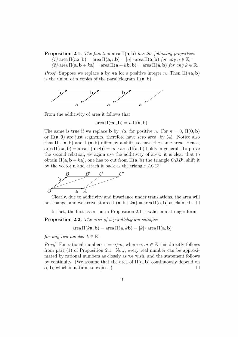
Proposition 2.1. The function area Π(a,b) has the following properties:(1) area Π(na,b) = area Π(a, nb) = |n| · area Π(a,b) for any n ∈ Z;(2) area Π(a,b + ka) = area Π(a + kb,b) = area Π(a,b) for any k ∈ R.

Proof. Suppose we replace a by na for a positive integer n. Then Π(na,b)is the union of n copies of the parallelogram Π(a,b):

-a

½½

½½>b

½½

½½

-a

½½

½½>b

½½

½½

-a

½½

½½>b

½½

½½

From the additivity of area it follows that

area Π(na,b) = n Π(a,b).

The same is true if we replace b by nb, for positive n. For n = 0, Π(0,b)or Π(a,0) are just segments, therefore have zero area, by (4). Notice alsothat Π(−a,b) and Π(a,b) differ by a shift, so have the same area. Hence,area Π(na,b) = area Π(a, nb) = |n| · area Π(a,b) holds in general. To provethe second relation, we again use the additivity of area: it is clear that toobtain Π(a,b + ka), one has to cut from Π(a,b) the triangle OBB′, shift itby the vector a and attach it back as the triangle ACC ′:

-O Aa

³³³³³³³³³1

³³³³³³³³³1

½½

½½>B C

b

½½

½½

C ′B′

Clearly, due to additivity and invariance under translations, the area willnot change, and we arrive at area Π(a,b+ka) = area Π(a,b) as claimed.

In fact, the first assertion in Proposition 2.1 is valid in a stronger form.

Proposition 2.2. The area of a parallelogram satisfies

area Π(ka,b) = area Π(a, kb) = |k| · area Π(a,b)

for any real number k ∈ R.

Proof. For rational numbers r = n/m, where n,m ∈ Z this directly followsfrom part (1) of Proposition 2.1. Now, every real number can be approxi-mated by rational numbers as closely as we wish, and the statement followsby continuity. (We assume that the area of Π(a,b) continuously depend ona, b, which is natural to expect.)

19

Theorem 2.1. Suppose a = (a1, a2), b = (b1, b2). Then

area Π(a,b) = C · |∆| , (1)

with some constant C, where

∆ = det(a,b) = det

(a1 a2

b1 b2

). (2)

Proof. Indeed, by Propositions 2.1 and 2.2, area Π(a,b) satisfies almost thesame properties as the determinant det(a,b). They can be used to calculatearea Π(a,b); it is similar to using row operations for calculating determinants.We have

area Π(a,b) = area Π

(a1 a2

b1 b2

)= area Π

(a1 a2

0 b2 − b1a1

a2

)=

area Π

(a1 0b1 b2 − b1

a1a2

)= |a1| |b2 − b1

a1

a2| area Π

(1 00 1

)=

|a1b2 − b1a2| · area Π(e1, e2) ,

where e1 = (1, 0) and e2 = (0, 1), as desired.

We see that the constant C in the theorem is the just area of the par-allelogram built on the ‘basis vectors’ e1, e2. Knowing this number allowsto calculate the area of any parallelogram by using formulas (1), (2). Thisnumber can be set arbitrarily, which is equivalent to a choice of the unit ofarea.

The meaning of Theorem 2.1 is very deep: it tells that the natural proper-ties of areas, such as additivity and invariance under translations, imply thatthe area of a parallelogram Π(a,b) has characteristic properties the same asthose of (the absolute value of) the determinant det(a,b). Therefore theyshould essentially coincide.

In the following examples let us assume that a unit of area is chosen sothat area Π(e1, e2) = 1.

Example 2.2. Find the area of the parallelogram built on vectors a =(−2, 5) and b = (1, 1). Solution: we have

∆ =

∣∣∣∣−2 51 1

∣∣∣∣ = −7 .

Hence area Π(a,b) = | − 7| = 7.

20

Example 2.3. Find the area of the triangle ABC if A = (3, 2), B = (4, 2),C = (1, 0). Solution: it is half of the area of the parallelogram built on−→CA = A− C = (2, 2),

−−→CB = B − C = (3, 2). Hence

area(ABC) =1

2

∣∣∣∣3 22 2

∣∣∣∣ = 1 .

How we can make sense of the determinant det(a,b) as such, not itsabsolute value? It corresponds to the notion of signed, or oriented area.Denote it Area Π(a,b) with capital “a”. By definition, signed area satisfies

Area Π(ka,b) = Area Π(a, kb) = k Area Π(a,b)

Area Π(a,b + ka) = Area Π(a + kb,b) = Area Π(a,b)

for all k ∈ R. We have

Area(a,b) =

∣∣∣∣a1 a2

b1 b2

∣∣∣∣ (3)

if we assume that the signed area of Π(e1, e2) equals 1.

2.2 Volumes and determinants

All the above results can be generalized to higher dimensions. Considervectors a1, . . . , an in Rn. The parallelipiped on a1, . . . , an with basepointO ∈ Rn is the set of points

x = O + t1a1 + . . . + tnan where 0 ≤ t1 ≤ 1 for all i = 1, . . . , n .

Denote it Π(a1, . . . , an). In the sequel nothing depends on the basepoint,so we shall suppress any mentioning of it. Instead of deducing a formulafor the volume of a parallelipiped similar to (1) from general properties ofvolumes such as additivity, as we did above for area, it is convenient to setby definition

Vol Π(a1, . . . , an) =

∣∣∣∣∣∣

a11 . . . a1n

. . . . . . . . .an1 . . . ann

∣∣∣∣∣∣(4)

if a1 = (a11, . . . , a1n), . . . , an = (an1, . . . , ann). This is the oriented or signedvolume. The ‘usual’ volume vol is the absolute value of Vol. Note that thisdefinition implies that the “unit of volume” is such that the oriented volumeof Π(e1, . . . , en) is set to 1.

21

Example 2.4. Find the oriented volume of the parallelipiped built on a1 =(2, 1, 0), a2 = (0, 3, 11) and a3 = (1, 2, 7) in R3. Solution:

Vol Π(a1, a2, a3) =

∣∣∣∣∣∣

2 1 00 3 111 2 7

∣∣∣∣∣∣= 2 · 1− 1 · 11 = −9 .

(The volume ‘without sign’ equals 9.)

2.3 Areas and volumes in Euclidean space

In the above analysis of areas and volumes, there was an arbitrary choiceof “unit of volume”, i.e., a choice of the constant before the determinant informulas such as (1), (3), (4). However, there is a natural choice linkingmeasurement of volumes and areas with measurement of lengths and angles.It is given by the rule: the volume of a unit cube equals 1. A unit cube in Rn

is a parallelipiped has unit edges that are perpendicular to each other. In R2

it is a unit square.Recall that on Rn one can define the scalar product of vectors by the

formula(a,b) = a1b1 + . . . + anbn

(see Problem 1.5). It follows that the ‘standard basis vectors’ e1, . . . , en

satisfy (ei, ej) = 0 if i 6= j and (ei, ei) = 1. The length of a vector is definedas

|a| =√

(a, a)

and the angle between two vectors is defined by the equality

(a,b) = |a| |b| cos α

from where we can find cos α if (a,b), (a, a), (b,b) are known. Hence therelations for ei mean that they all have unit length and are mutually per-pendicular. Therefore Π(e1, . . . , en) is a unit cube. We set

Vol Π(e1, . . . , en) = 1 .

Then for any n vectors ai = (ai1, . . . , ain), where i = 1, . . . , n, we obtain

Vol Π(a1, . . . , an) =

∣∣∣∣∣∣

a11 . . . a1n

. . . . . . . . .an1 . . . ann

∣∣∣∣∣∣. (5)

22

Remark 2.1. The space Rn together with the scalar product is called then-dimensional Euclidean space. The adjective ‘Euclidean’ points to the factthat the scalar product allows to define lengths and angles, i.e., the mainnotions of the classical Euclidean geometry.

Remark 2.2. The scalar product is alternatively denoted a ·b and hence isoften referred to as the ‘dot product’.

It seems that the unit cube Π(e1, . . . , en) plays a distinguished role. Laterwe shall show that any unit cube in Rn has unit volume. Consider an example(for n = 2 we continue to use Area instead of Vol).

Example 2.5. Let g1 = (cos α, sin α), g2 = (− sin α, cos α) in R2. We canimmediately see that |g1| = |g2| = 1 and g1 · g2 = 0, so Π(g1,g2) is a unitsquare. We have

Area Π(g1,g2) =

∣∣∣∣cos α sin α− sin α cos α

∣∣∣∣ = cos2 α + sin2 α = 1.

There is a way of expressing the volume of a parallelipiped entirely interms of ‘intrinsic’ geometric information: lengths of vectors and angles be-tween them, rather than their coordinates as in the previous formulas. Con-sider the matrix

G(a1, . . . , ak) =

(a1, a1) . . . (a1, ak). . . . . . . . .

(ak, a1) . . . (ak, ak)

. (6)

Here k ≤ n may be less than n.

Definition 2.1. The matrix G(a1, . . . , an) is called the Gram matrix of thesystem of vectors a1, . . . , an and its determinant, the Gram determinant.

Theorem 2.2. The Gram determinant of a1, . . . , an is the square of thevolume of the parallelipiped Π(a1, . . . , an).

Proof. Indeed, consider the n× n matrix A with rows ai. Consider

AAT =

a11 . . . a1n

. . . . . . . . .an1 . . . ann

a11 . . . an1

. . . . . . . . .a1n . . . ann

=

a1

. . .an

(

aT1 . . . aT

n

)=

a1aT1 . . . a1a

Tn

. . . . . . . . .ana

T1 . . . ana

Tn

= G(a1, . . . , an) .

23

Hence

det G(a1, . . . , an) = det(AAT ) = det A det AT =

(det A)2 =(vol Π(a1, . . . , an)

)2

.

Corollary 2.1. If gi, i = 1, . . . , n, are arbitrary mutually orthogonal unitvectors (i.e., Π(g1, . . . ,gn) is a unit cube), then vol Π(g1, . . . ,gn) = 1.

Proof. Indeed,(vol Π(g1, . . . ,gn)

)2

= det G(g1, . . . ,gn)) = det E = 1.

One of the advantages of expressing volumes via the Gram determinants isthat it allows to consider easily parallelipipeds in Rn of dimensions less thann. More precisely, if we are given k vectors a1, . . . , ak, then we can considera k-dimensional parallelipiped Π(a1, . . . , ak) contained in the k-dimensionalplane spanned by a1, . . . , ak. The formula

(vol Π(a1, . . . , ak)

)2

= det G(a1, . . . , ak)

is applicable, with the scalar products calculated in the ambient space Rn.

Example 2.6. Find the area of the parallelogram built on a = (1,−1, 2)and b = (2, 0, 3). Solution: the Gram determinant is

∣∣∣∣6 88 13

∣∣∣∣ = 14 .

Hence the area is√

14.

Remark 2.3. Differently from the case of an n-dimensional parallelipiped inRn, where one can consider ‘signed’ volume given by formula (4), the volumeof a k-dimensional parallelipiped, for k < n, given by the Gram determinantis not signed. (For k = n, if we use the Gram determinant, to obtain a signedvolume, we have to pick a sign independently.)

For n = 2, it is obvious that the area of a parallelogram Π(a,b) is theproduct of the ‘base’ |a| and ‘height’ h, which is the length of a vectorh = b + ka such that it is perpendicular to a (the parameter k is defined

24

by the condition (a,h) = 0). It is a very basic fact following from thesame sort of ideas that lead us to discovering the relation between areas anddeterminants. For n = 3, the similar fact about the volume of a 3-dimensionalparallelipiped is also very familiar. This relation between the n-dimensionalvolume in the Euclidean space Rn and the (n−1)-dimensional volume in theEuclidean space Rn−1 holds for any n. The easiest way to prove it is by usingthe Gram determinants.

Temporarily introduce notation voln and voln−1 for distinguishing be-tween volumes in Rn and Rn−1. Let us consider the (n− 1)-dimensional par-allelipiped Π(a1, . . . , an−1) as a base of a parallelipiped Π(a1, . . . , an). Thenthe height of Π(a1, . . . , an) is the length of a (unique) vector h defined bythe condition h = an + c where c is a linear combination of a1, . . . , an−1 andh is perpendicular to the plane of a1, . . . , an−1 (i.e., to each of the vectorsa1, . . . , an−1).

Theorem 2.3. The following formula holds:

voln Π(a1, . . . , an) = voln−1 Π(a1, . . . , an−1) · h ,

where h = |h| is the height of Π(a1, . . . , an).

Proof. Using the properties of volumes we immediately conclude that

voln Π(a1, . . . , an) = voln Π(a1, . . . , an−1,h).

Now we can apply the Gram determinant:

det G(a1, . . . , an−1,h) =

∣∣∣∣∣∣∣∣

(a1, a1) . . . (a1, an−1) (a1,h). . . . . . . . . . . .

(an−1, a1) . . . (an−1, an−1) (an−1,h)(h, a1) . . . (h, an−1) (h,h)

∣∣∣∣∣∣∣∣=

∣∣∣∣∣∣∣∣

(a1, a1) . . . (a1, an−1) 0. . . . . . . . . . . .

(an−1, a1) . . . (an−1, an−1) 00 . . . 0 (h,h)

∣∣∣∣∣∣∣∣= det G(a1, . . . , an−1) · |h|2 .

and it remains to extract the square root.

2.4 Examples and applications

Consider two applications of the methods introduced above.

25

2.4.1 The distance between a point and a plane

Consider a plane L in R3 and a point x not belonging to L. What is thedistance between x and L? It is natural to define it as the minimum of thedistances between x and points of the plane L. A practical calculation ofit can be nicely related with areas and volumes. Indeed, let y ∈ L is anarbitrary point of the plane; the distance between x and y is |x − y|. Wecan write x − y = a‖ + a⊥ where the vector a‖ is parallel to L and a⊥ isperpendicular to it. Hence |x− y|2 = |a‖|2 + |a⊥|2 ≥ |a⊥|2. The part a‖ canvary by adding vectors parallel to L, while a⊥ is unique as long as x is given.It is clear now that the shortest length so obtained is for x − y = a⊥, i.e.,when y is the end of the perpendicular dropped on L from the point x. (Drawa picture.) Let O be some fixed point of the plane L and let vectors a1, . . . , ak

‘span’ L so that an arbitrary point of L has the appearance O + c1a1 + . . . +ckak. Then we can consider a k-dimensional parallelipiped Π(a1, . . . , ak) anda (k+1)-dimensional parallelipiped Π(a1, . . . , ak,x−O), both with basepointO. Clearly, the desired distance is the height of Π(a1, . . . , ak,x−O).

Corollary 2.2. The distance between a point x and a plane L through apoint O in the direction of vectors a1, . . . , ak is given by the formula

vol Π(a1, . . . , ak,x−O)

vol Π(a1, . . . , ak)=

√det G(a1, . . . , ak,x−O)√

det G(a1, . . . , ak)

Example 2.7. Given a plane through the points A = (1, 0, 0), B = (0, 1, 0),C = (0, 0, 1). Find the distance between it and the point D = (3, 2,−1).

Solution: denote the desired distance by h. Consider the vectors a =−→CA =

(1, 0,−1), b =−−→CB = (0, 1,−1) and d =

−−→CD = (3, 2,−2). We have

h =vol Π(a,b,d)

area Π(a,b).

The numerator is easier to find by using formula (4). We have∣∣∣∣∣∣

1 0 −10 1 −13 2 −2

∣∣∣∣∣∣=

∣∣∣∣1 −12 −2

∣∣∣∣−∣∣∣∣0 13 2

∣∣∣∣ = 3

hence vol Π(a,b,d) = 3. For the denominator we calculate the Gram deter-minant:

det G(a,b) =

∣∣∣∣(a, a) (a,b)(b, a) (b,b)

∣∣∣∣ =

∣∣∣∣2 11 2

∣∣∣∣ = 1 ;

26

hence area Π(a,b) =√

det G(a,b) = 1. Finally, h = 3.

2.4.2 Area of a piece of the plane or a surface

Knowing how to find the area of a parallelogram allows to find the areas ofmore general objects. The same is true for volumes in higher dimensions.

Consider first the problem of calculating the area of a domain in R2 usingso-called “curvilinear coordinates”. By a system of curvilinear coordinatesin a part of the plane R2 is understood a way of specifying points x = (x, y)by suitable parameters u, v instead of their ‘standard’ coordinates x, y.

Example 2.8. Polar coordinates r, θ where x = r cos θ, y = r sin θ.

Let us choose such a system u, v. Curves v = const and u = const arecalled coordinate lines. For example, for standard coordinates x, y they arehorizontal and vertical lines, respectively. For polar coordinates r, θ they arerays emanating from the origin O = (0, 0) and circles with center O.

Consider a region of the plane bounded by the coordinate lines v = v0,v = v0 + ∆v, u = u0 and u = u0 + ∆u. For small increments ∆u, ∆v itis a ‘curvilinear quadrangle’ with the vertices A where u = u0, v = v0, Bwhere u = u0 + ∆u, v = v0, C where u = u0 + ∆u, v = v0 + ∆v, and Dwhere u = u0, v = v0 + ∆v. Denote its area by ∆S. For small ∆u, ∆v, thiscurvilinear quadrangle ABCD is very close to the parallelogram built on thevectors

a = eu ∆u, b = ev ∆v

where eu = ∂x∂u

(u0, v0), ev = ∂x∂v

(u0, v0), with basepoint A. (Draw a picture!)Hence the area ∆S can be approximated by

area Π(eu ∆u, ev ∆v) = area Π(eu, ev)∆u∆v =√

det G(eu, ev) ∆u∆v

Denote for brevity det G(eu, ev) by g. It is a function of a point in the plane.

Example 2.9. (Continuation of Example 2.8.) We have, for polar coordi-nates,

er =∂x

∂r= (cos θ, sin θ), eθ =

∂x

∂θ= (−r sin θ, r cos θ) .

Hence

G(er, eθ) =

(er · er er · eθ

eθ · er eθ · eθ

)=

(1 00 r2

)

and g = det G(er, eθ) = r2.

27

How can we use this? Suppose we want to calculate the area of a certaindomain D ⊂ R2. Choose some system of curvilinear coordinates in which Dcan be conveniently described. Consider a partition of D by the coordinatelines v = vk, u = ul, k, l = 1, . . . , N , where ul+1 − ul = ∆u, vk+1 − vk =∆v. Then the area of D is approximated by the sum of the areas of thecurvilinear quadrangles ∆S as above, where u varies between ul and ul+1,and v, between vk and vk+1. We can also approximate each of ∆S by thearea of the parallelogram Π(eu∆u, ev∆v). The basepoints are on the grid,and the vectors eu, ev are calculated at the corresponding points of the grid.Hence

area D = lim∑

k,l

∆S = lim∑

k,l

area Π(eu∆u, ev∆v) = lim∑

k,l

√g∆u∆v

where g = det G(eu, ev). It is just the integral sum for a double integral, andwe arrive at the following statement.

Proposition 2.3. For the area of a domain D ⊂ R2 we have

area D =

∫∫

D

dS where dS =√

gdudv .

The expression dS under the integral sign is called the element of area.

Example 2.10. The element of area in the standard coordinates x, y andpolar coordinates r, θ will be

dS = dxdy = rdrdθ

using the result of Example 2.9.

Example 2.11. Find the area of a disk DR of radius R using the aboveformulas. Solution: let the center of the disk be at the origin; in polarcoordinates we have 0 ≤ r ≤ R, 0 ≤ θ ≤ 2π, and

area DR =

∫∫

DR

dS =

∫∫

DR

rdrdθ =

∫ 2π

0

dθ

∫ R

0

rdr = 2π1

2R2 = πR2.

Example 2.12. Similarly, for a sector of the same disk, of angle ∆θ, we have(denoting the sector by S)

area S =

∫∫

S

dS =

∫∫

S

rdrdθ =

∫ ∆θ

0

dθ

∫ R

0

rdr =1

2R2 ∆θ.

28

Exactly in the same way this works for pieces of surfaces in R3. If asurface M is parametrized by parameters u, v, then we again have vectors

eu =∂x

∂u, ev =

∂x

∂v,

which are now in the tangent planes at points of M (so they vary from pointto point). We have parallelograms Π(eu∆u, ev∆v) in the tangent planes,approximating infinitesimal pieces of the surface M . Hence for the elementof area we have the same formula

dS =√

g dudv where g = det G(eu, ev) ,

and the area of (a piece of) M is given by a double integral:

area M =

∫∫

M

dS =

∫∫

M

√g dudv .

Example 2.13. Points x = (x, y, z) of the sphere of radius R with center atthe origin can be parametrized by angles θ, ϕ, where 0 ≤ θ ≤ π, 0 ≤ ϕ ≤ 2π,as follows: x = R sin θ cos ϕ, y = R sin θ sin ϕ, z = R cos θ. Hence we obtain

eθ =∂x

∂θ= (R cos θ cos ϕ,R cos θ sin ϕ,−R sin θ)

eϕ =∂x

∂ϕ= (−R sin θ sin ϕ,R sin θ cos ϕ, 0) .

An immediate calculation gives the following Gram matrix:

G(eθ, eϕ) =

(eθ · eθ eθ · eϕ

eϕ · eθ eϕ · eϕ

)=

(R2 00 R2 sin2 θ

).

Hence g = R4 sin2 θ, and for the element of area for the sphere we get

dS = R2 sin θ dθdϕ.

2.5 Problems

Problem 2.1. Find the areas and volumes (signed where indicated):(a) Area Π(a,b) if a = (− cos α,− sin α), b = (− sin α, cos α) in R2; make asketch;(b) Vol Π(a,b, c) if a = (3, 2,−1), b = (2, 2, 5), c = (0, 0, 1) in R3;(c) area(a,b) if a = (1,−1, 2, 3), b = (0, 3, 1, 2) in R4.(Ans.: (a) −1; (b) 2; (c) 15.)

29

Problem 2.2. Verify by a direct calculation that the Gram determinantdet G(a,b, c) vanishes if one of the vectors a,b, c is a linear combinationof the others. (Geometrically that means that they are in the same plane.)What can be said about the volume of the parallelipiped Π(a,b, c)?

Problem 2.3. Show that the oriented area of a triangle ABC in R2 is givenby the formula

area(ABC) =1

2

∣∣∣∣∣∣

A1 A2 1B1 B2 1C1 C2 1

∣∣∣∣∣∣if A = (A1, A2), B = (B1, B2), C = (C1, C2).

Problem 2.4. (See Problem 1.5.)(a) Show that the so-called triple or mixed product (a,b, c) in R3 defined asa · (b× c) = (a× b) · c is the oriented volume of Π(a,b, c).(b) Apply the result of part (a) to prove that the length of the vector producta× b in R3 is the area of the parallelogram Π(a,b).Hint: for part (b), consider the parallelipiped Π(a,b,n) where n is a unitvector perpendicular to a and b, and apply Theorem 2.3.

Problem 2.5. Show that |a×b| = |a| |b| ·sin α where α is the angle betweena and b.Hint: use the result of the previous problem, part (b), and express the areaby the Gram determinant.

Problem 2.6. Show that the distance of a point C = (C1, C2) from thestraight line passing through points A = (A1, A2) and B = (B1, B2) in theplane is given by the absolute value of the expression

1

|B − A|

∣∣∣∣∣∣

A1 A2 1B1 B2 1C1 C2 1

∣∣∣∣∣∣.

Problem 2.7. Find the area of the sphere S2R : x2 + y2 + z2 = R2 as the

integral∫∫

S2R

dS using the result of Example 2.13. (Answer: 4πR2.)

30