International Review of Economics and Finance 45 (2016) 16–32

Contents lists available at ScienceDirect

International Review of Economics and Finance

j ourna l homepage: www.e lsev ie r .com/ locate / i re f

Determinacy and learnability of equilibrium in a small-openeconomy with sticky wages and prices

Eurilton Araújo ⁎Central Bank of Brazil, Brasília, Brazil FUCAPE Business School, Vitória, Brazil

a r t i c l e i n f o

⁎ Central Bank of Brazil, Research Department, Setor BE-mail address: eurilton@gmail.com.

http://dx.doi.org/10.1016/j.iref.2016.04.0141059-0560/© 2016 Elsevier Inc. All rights reserved.

a b s t r a c t

Article history:Received 27 July 2015Received in revised form 27 April 2016Accepted 27 April 2016Available online 5 May 2016

In a small-open economy model with nominal wage and price rigidities, it has been arguedthat, in terms of welfare losses, the monetary policy rule that responds to consumer priceindex (CPI) inflation performs better than rules that react to competing inflation measures.From the viewpoint of determinacy and learnability of rational expectations equilibrium(REE), this paper suggests that the rule that responds to CPI inflation does not increase theCentral Bank's ability to promote the convergence of an economy to a determinate and learn-able REE nor improves the speed of this convergence when compared with rules that react tocontending inflation measures.

© 2016 Elsevier Inc. All rights reserved.

JEL Classification:E13E31E52F41

Keywords:DeterminacyInflationLearnabilityMonetary policy rules

1. Introduction

Despite the behavior of many inflation-targeting central banks, most research on small-open economies with sticky prices,such as Gal and Monacelli (2005), suggests that the monetary authority should respond to domestic inflation rather than toconsumer price index (CPI) inflation. In a small open economy with sticky wages and prices, Rhee and Turdaliev (2013) andCampolmi (2014) compared monetary policy rules that reacted to different inflation measures according to their welfare losses.In this context, they found that CPI inflation performed better than some contending measures, including domestic inflation.

Sticky nominal wages alter the dynamics of the Gal and Monacelli (2005) model. In the presence of nominal wage rigidity,fluctuations in CPI inflation induce movements in real wages, which affect wage markups. Hence, changes in wage markupslead to fluctuations in wage inflation and in firms' marginal costs. Therefore, in contrast to Gal and Monacelli (2005), there is adirect effect of CPI inflation on domestic price inflation.

In addition, since CPI inflation depends on movements in the real exchange rate or in the terms of trade, foreign shocks, bychanging these variables, immediately influence domestic inflation dynamics. This mechanism is the direct exchange rate channelto domestic price inflation. This channel emerges through staggered wage contracting in small open economies and it is absent instandard new Keynesian open-economy models without sticky nominal wages.

ancário Sul (SBS), Quadra 3, Bloco B, Edifcio-Sede, Brasilia DF 70074-900, Brazil.

17E. Araújo / International Review of Economics and Finance 45 (2016) 16–32

As pointed out by Campolmi (2014), in response to domestic and foreign shocks, movements in CPI inflationtranslate into more volatile wage and domestic inflation rates. In this context, the central bank improves welfare byreacting to CPI inflation since this reaction reduces the volatility of wage inflation and the volatility of domesticinflation. By decreasing these volatilities, the central bank promotes reductions in wage and price dispersions, whichenhance welfare.

In addition to its repercussion on welfare, the change in model dynamics engendered by the introduction of sticky nominalwages has potential implications for determinacy and E-stability of REE in small open economies. The investigation of theseimplications is therefore the goal of this paper.

Since researchers have also assessed the desirability of an interest rate rule by examining the determinacy and learnabilityproperties that this rule induces in equilibrium, the main contribution of this paper is to revisit, from the perspective ofdeterminacy and learnability of rational expectations equilibrium (REE), the following question: which inflation index shouldmonetary policy rules react to?

In contrast to Rhee and Turdaliev (2013) and Campolmi (2014), I emphasize determinacy and learnability properties asperformance criteria to address the question of which inflation measure should a central bank respond to. Indeed, I presentnumerical results on determinacy and E-stability of equilibria for a small open economy model with sticky nominal wages andprices in which interest rate rules respond to alternative inflation measures.

This paper also addresses the effects of introducing nominal wage rigidity and trade openness on determinacy and learnabilityconditions associated with competing interest rate rules. Moreover, following Ferrero (2007) and Christev and Slobodyan (2014),I investigate how the specification of interest rate rules matters for the speed of convergence of an economy to a determinateand E-stable REE through an adaptive learning process. In fact, the speed of learning is an additional yardstick through whichI evaluate monetary policy rules.

The main finding of this paper suggests that, when compared with rules that react to competing inflation measures,the rule that responds to CPI inflation does not provide any noticeable improvement in the central bank's ability topromote convergence of an economy to a determinate and learnable REE. Moreover, for this rule, the learning algorithmconverges slowly or with the same speed implied by alternative rules. Hence, in contrast to the evaluation based onwelfare losses, the rule that responds to CPI inflation does not exhibit superior performance from the viewpoint ofdeterminacy and E-stability.

This study is closely related to Llosa and Tuesta (2008) and Best (2015). Llosa and Tuesta (2008) studied the small openeconomy model developed by Gal and Monacelli (2005) and showed that the degree of openness interacted with particularinterest rate rules, which may respond to exchange rates, to change the relevance of the Taylor principle as a condition ensuringdeterminacy and E-stability of REE. In a previous paper, Linnemann and Schabert (2006) found similar results by studying a morerestricted class of interest rate rules. Best (2015)1 studied a closed economy model with nominal wage and price rigidities asdescribed in Erceg, Henderson, and Levine (2000).

The paper proceeds as follows. Section 2 sets out the model. Section 3 presents the numerical findings on determinacy andE-stability of REE. Section 4 discusses the speed of convergence of determinate and E-stable equilibria. Finally, the lastsection concludes.

2. The model

In this section, I present the log-linear approximation of the model investigated in Rhee and Turdaliev (2013) and Campolmi(2014)2. This model is the small-open economy studied in Gal and Monacelli (2005) with the labor market characteristics foundin Erceg et al. (2000), i.e., there is monopolistic competition in the labor market and households set nominal wages following thescheme proposed by Calvo (1983)3. I also discuss alternative interest rate rules representing how the central bank conductsmonetary policy and I then report how I calibrate the parameters.

2.1. The private sector equilibrium conditions

After the log-linearization around the steady state of the equilibrium conditions exposed in Appendix A, the followingequations represent the small open economy:

1 Flas2 Llos

rigidity3 Reg

type of

~yt ¼ Et ~ytþ1� �

−1σα

rt−Et πH;tþ1

� �h iþ 1σα

rrnt ð1Þ

πH;t ¼ βEt πH;tþ1

� �þ κph~yt þ λph ~wt ð2Þ

chel, Franke, and Proaño (2008) studied a similar model in continuous time.a and Tuesta (2008) and Best (2015) are special cases of this model. In fact, the model in Llosa and Tuesta (2008) corresponds to setting the degree of wageto zero whereas the specification in Best (2015) is equivalent to the situation of zero degree of openness.arding the introduction of nominalwage rigidity, Adolfson, Lassén, Lindé, andVillani (2008); Jääskelä andNimark (2011), andDong (2013) pointed out that thisnominal rigidity improved the ability of open-economy medium-scale models to fit the data.

4 Theural lev

5 TheExpress

6 The7 Rhe

18 E. Araújo / International Review of Economics and Finance 45 (2016) 16–32

πW;t ¼ βEt πW;tþ1

� �þ κw~yt − λw ~wt ð3Þ

~wt ¼ ~wt−1 þ πW;t − πCPI;t −Δwnt ð4Þ

πCPI;t ¼ πH;t þ α st − st−1ð Þ ð5Þ

~yt ¼1σα

st þ y�t − ynt ð6Þ

The endogenous variables ~yt, πH ,t, πW ,t, ~wt, rt, πCPI ,t, and st stand for the domestic output gap, domestic inflation, nominal wageinflation, the real wage gap, the domestic interest rate, CPI inflation, and the terms of trade. The exogenous variables rrtn, Δwt

n, ytn,and y t

⁎ denote the natural level of the real interest rate, the variation in the natural real wage, the natural level of output andforeign output.4 I assume that mutually independent first-order autoregressive processes characterize the dynamics of rrtn, Δwt

n,and yt

n, while keeping yt⁎ constant at its steady state level.

The Euler equation is expression (1), which summarizes households' intertemporal consumption decisions. Eq. (2) defines thenew Keynesian Phillips curve and sums up the price-setting behavior of monopolistic firms. Eq. (3) characterizes the evolution ofthe wage inflation and Eq. (4) describes real wage dynamics. These expressions are implications of households' optimal wagesetting. Finally, Eq. (5) defines CPI inflation and Eq. (6) results from the assumption of complete markets and market clearingconditions in the domestic economy.5 The expectation operator Et represents rational expectations as well as alternativeexpectation formation mechanisms.

The inspection of Eqs. (2)–(5) reveals how the direct exchange rate channel operates. In Eq. (4), movements in CPI inflationaffect the real wage gap, which directly influences domestic price inflation and wage inflation through Eqs. (2) and (3). Eq. (5)shows that endogenous movements in the terms of trade can trigger variations in CPI inflation with an immediate effect ondomestic price inflation.6

The parameter β stands for the discount factor, σ measures the degree of relative risk aversion, φ is the inverse of the laborsupply elasticity, γ is the elasticity of substitution between imported goods, η is the elasticity of substitution between domesticand foreign goods, and α measures the degree of trade openness. The degrees of price and wage stickiness are θph and θw. Finally,the parameter εw stands for the elasticity of substitution between distinct types of labor in the monopolistic competitivelabor market.

The symbols λph, λw, Ω, σα, κph, and κw denote convolutions of the deep parameters. The expressions defining them are:

λph ¼1− θph� �

1− βθph� �θph

;λw ¼ 1− θwð Þ 1− βθwð Þθw 1þ εwφð Þ ;Ω ¼ γσ þ 1−αð Þ ησ − 1ð Þ;

σα ¼ σ1−αð Þ þ αΩ

; κph ¼ ασαλph and κw ¼ σ −ασαΩþ φð Þλw:

2.2. Monetary policy

I assume that the central bank follows an interest rate rule. As in Llosa and Tuesta (2008), I consider two alternativespecifications for interest rate rules: contemporaneous data and forecast-based data.

The expression for the contemporaneous specification is

rt ¼ ϕrrt−1 þ ϕpπm;t þ ϕy~yt ð7Þ

The forecast-based data interest rate rule is

rt ¼ ϕrrt−1 þ ϕpEtπm;tþ1 þ ϕyEt~ytþ1 ð8Þ

The variable πm , t stands for some particular inflation measure m. I consider the following inflation measures: domesticinflation (πH ,t ), CPI inflation (πCPI ,t), and nominal wage inflation (πW ,t).7 The parameters describing the rules are ϕr, capturinginterest rate inertia, and the coefficients ϕp and ϕy reflecting the response of the interest rate to the variables πm ,t and ~yt or,in forecast-based rules, to their expected future values. For each rule above, I consider two cases: the benchmark situation(ϕr=0) and the interest rate smoothing specification (ϕr=0.65).

natural level of an economic variable is its equilibrium value in the absence of nominal rigidities. The gap is the difference between a given variable and its nat-el.correspondence between expressions (1)–(6) and the equations in Rhee and Turdaliev (2013) goes as follows. Expression (6) is equation (16) on page 312.ions (2) and (3) are equations (22) and (23) on page 313. Finally, expressions (1), (4) and (5) are on page 314.expression qt=(1−α)st relates the real exchange rate (qt) to the terms of trade (st). Hence, these variables move in tandem.e and Turdaliev (2013) and Campolmi (2014) looked at these three inflation indices.

19E. Araújo / International Review of Economics and Finance 45 (2016) 16–32

Eqs. (1)–(6) and a given interest rate rule comprise the dynamic system of equations that summarizes the artificial economyin Rhee and Turdaliev (2013). To study determinacy and learnability of REE, I parsimoniously represent this system by substitut-ing out some endogenous variables. Appendix B discusses the system reduction and shows the matrices characterizing the parsi-monious representation.

2.3. Calibration

In the baseline calibration of the model, I choose the parameters as follows.

• Preferences. Following Rhee and Turdaliev (2013) and Campolmi (2014), I set the elasticity of labor supply to 13 by specifying φ=3,

and the discount factor is β=0.99. The coefficient of risk aversion is σ=5,which is the value employed by Llosa and Tuesta (2008).• Goods and labor markets. Again, I stick to the values found in Rhee and Turdaliev (2013) and Campolmi (2014). Therefore, εw=6and θph=θw=0.75.

• Open-economy parameters. Following Gal and Monacelli (2005); Llosa and Tuesta (2008) and Campolmi (2014), I set α=0.4.Agreeing with Llosa and Tuesta (2008), I set γ=1 and η=1.5.

3. Determinacy and E-stability

Equilibrium determinacy and learnability, also known as expectational stability (E-stability), have become important criteriafor the design and evaluation of monetary policy rules in new Keynesian models. By definition, a determinate REE is unique,free from self-fulfilling fluctuations, and non-explosive. In addition, a REE is E-stable if agents who do not initially possess rationalexpectations coordinate upon it after using least-squares adaptive learning methods to acquire knowledge about the law ofmotion governing macroeconomic dynamics.

Evans and Honkapohja (2001) and Bullard and Mitra (2002, 2007) provided the foundations to analyze determinacy andE-stability of equilibria under the assumption of rational expectations. Since the publication of these papers, a burgeoningliterature examining conditions that ensure determinacy and E-stability of REE in extensions of the new Keynesian model hasemerged.8 Next, I summarize the conditions for determinacy and learnability in Evans and Honkapohja (2001).

3.1. Methodology

I consider the following system of linear stochastic difference equations:

8 Justrole of lnacy an

xt ¼ BEtxtþ1 þ Dxt−1 þ Kvtvt ¼ Rvt−1 þ ζ t

where xt is a m×1 vector of endogenous variables and vt is a k×1 vector of exogenous disturbances.For determinacy analysis, I write the system above in the following compact form:

Etztþ1 ¼ J1zt þ J2vt

where J1 and J2 are functions of the matrices defining the original system and zt=[xtxt−1]′.According to Farmer (1999), the REE is determinate if the number of stable eigenvalues of J1 is equal to the number of

predetermined variables in zt.The method for E-stability analysis follows the standard approach of Evans and Honkapohja (2001), which I summarize below.Under adaptive learning, economic agents use recursive least-squares updating to form expectations. They have a forecasting

model known as the perceived law of motion (PLM), which is based on the MSV (minimum state variable) solution of the linearsystem of rational expectations.

The MSV solution has the form: xt=a+bxt−1+cvt, where a is m×1, b is m×m, and c is m×k.The assumptions about agents' information set at time t are important in deriving E-stability conditions. In this paper, the

information set is the same used in Llosa and Tuesta (2008) and Best (2015) and corresponds to the vector (1,x′t−1,vt ′)′.Under this time t information set, the expectations are Etxt+1=(I+b)a+b2xt−1+(bc+cR)vt, where I denotes the identitymatrix.

The insertion of the expectations Etxt+1 above in the original system gives the actual law of motion (ALM):

xt ¼ B I þ bð Þaþ Bb2 þ D� �

xt−1 þ Bbcþ BcRþ Kð Þvt

to cite a few papers: Duffy and Xiao (2011) investigated the effects of capital accumulation, Kurozumi and Van Zandweghe (2012) and Best (2015) studied theabor market frictions. Finally, Linnemann and Schabert (2006), Llosa and Tuesta (2008), and Bullard and Schaling (2009) exemplified the research on determi-d learnability of equilibria in open-economy models.

20 E. Araújo / International Review of Economics and Finance 45 (2016) 16–32

The perceived law of motion (PLM) used in the least-squares learning algorithm is the MSV solution and the map from PLMto ALM is

9 The10 This(2012).11 The

T a; b; cð Þ ¼ B I þ bð Þa;Bb2 þ D;Bbcþ BcRþ K� �

The vector ða; b; cÞ is the fixed point of the map from PLM to ALM, known as the T-map, and corresponds to a REE of theoriginal system.

Evans and Honkapohja (2001) stated the conditions for E-stability, governing the convergence of the least-squares learningalgorithm to a REE. To check these conditions, I have to compute the following derivativematrices9:DTaða; bÞ ¼ BðI þ bÞ,DTbðbÞ ¼b⊗Bþ I⊗Bb, and DTcðb; cÞ ¼ R0⊗bþ I⊗Bb, where the operator ⊗ denotes the Kronecker product. Finally, the REE solution of theoriginal system is E-stable or learnable under the following conditions: all real parts of the eigenvalues of the derivative matricesabove are lower than 1.

3.2. Results

The derivation of analytical results is not always possible, except in some special cases, such as the small open economy modelinvestigated in Llosa and Tuesta (2008). Indeed, the addition of sticky nominal wages increases the dimension of the system andposes great challenges for dimension reduction, which would facilitate analytical results. For this reason, I adopt a simulationapproach and provide numerical findings.10

Figs. 1–6 show the regions of determinacy and E-stability associated with alternative specifications for monetary policy rulesdescribed by Eqs. (7) and (8).11 Under the baseline calibration, I investigate a benchmark rule in which I fix ϕr=0 and a rule withinterest rate smoothing (IRS) in which I set ϕr=0.65, following the specification in Best (2015).

Moreover, I also study how the combination of staggered wage contracts and the degree of trade openness affects determinacyand learnability areas. In fact, these features are responsible for the emergence of the direct exchange rate channel discussed inthe introduction.

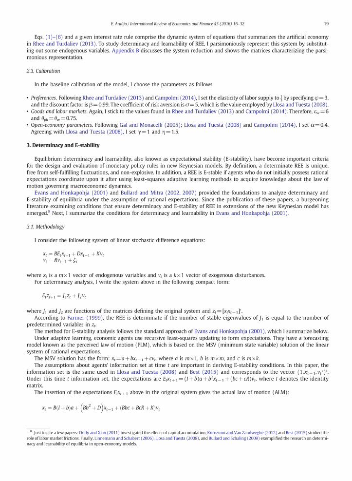
3.2.1. Contemporaneous data rulesFig. 1 illustrates the regions of determinacy and E-stability for the contemporaneous specification of the interest rate rule under

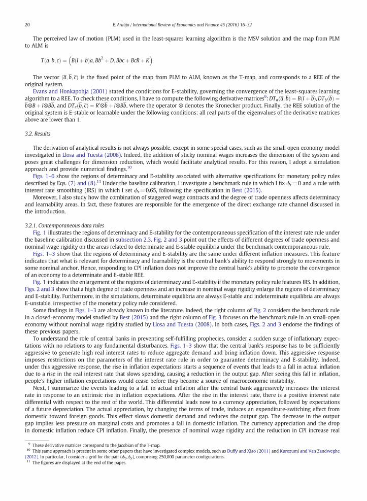
the baseline calibration discussed in subsection 2.3. Fig. 2 and 3 point out the effects of different degrees of trade openness andnominal wage rigidity on the areas related to determinate and E-stable equilibria under the benchmark contemporaneous rule.

Figs. 1–3 show that the regions of determinacy and E-stability are the same under different inflation measures. This featureindicates that what is relevant for determinacy and learnability is the central bank's ability to respond strongly to movements insome nominal anchor. Hence, responding to CPI inflation does not improve the central bank's ability to promote the convergenceof an economy to a determinate and E-stable REE.

Fig. 1 indicates the enlargement of the regions of determinacy and E-stability if the monetary policy rule features IRS. In addition,Figs. 2 and 3 show that a high degree of trade openness and an increase in nominal wage rigidity enlarge the regions of determinacyand E-stability. Furthermore, in the simulations, determinate equilibria are always E-stable and indeterminate equilibria are alwaysE-unstable, irrespective of the monetary policy rule considered.

Some findings in Figs. 1–3 are already known in the literature. Indeed, the right column of Fig. 2 considers the benchmark rulein a closed-economy model studied by Best (2015) and the right column of Fig. 3 focuses on the benchmark rule in an small-openeconomy without nominal wage rigidity studied by Llosa and Tuesta (2008). In both cases, Figs. 2 and 3 endorse the findings ofthese previous papers.

To understand the role of central banks in preventing self-fulfilling prophecies, consider a sudden surge of inflationary expec-tations with no relations to any fundamental disturbances. Figs. 1–3 show that the central bank's response has to be sufficientlyaggressive to generate high real interest rates to reduce aggregate demand and bring inflation down. This aggressive responseimposes restrictions on the parameters of the interest rate rule in order to guarantee determinacy and E-stability. Indeed,under this aggressive response, the rise in inflation expectations starts a sequence of events that leads to a fall in actual inflationdue to a rise in the real interest rate that slows spending, causing a reduction in the output gap. After seeing this fall in inflation,people's higher inflation expectations would cease before they become a source of macroeconomic instability.

Next, I summarize the events leading to a fall in actual inflation after the central bank aggressively increases the interestrate in response to an extrinsic rise in inflation expectations. After the rise in the interest rate, there is a positive interest ratedifferential with respect to the rest of the world. This differential leads now to a currency appreciation, followed by expectationsof a future depreciation. The actual appreciation, by changing the terms of trade, induces an expenditure-switching effect fromdomestic toward foreign goods. This effect slows domestic demand and reduces the output gap. The decrease in the outputgap implies less pressure on marginal costs and promotes a fall in domestic inflation. The currency appreciation and the dropin domestic inflation reduce CPI inflation. Finally, the presence of nominal wage rigidity and the reduction in CPI increase real

se derivative matrices correspond to the Jacobian of the T-map.same approach is present in some other papers that have investigated complex models, such as Duffy and Xiao (2011) and Kurozumi and Van ZandwegheIn particular, I consider a grid for the pair (ϕp,ϕy), comprising 250,000 parameter configurations.figures are displayed at the end of the paper.

Fig. 1. Contemporaneous data rule: baseline calibration.

21E. Araújo / International Review of Economics and Finance 45 (2016) 16–32

wages. Higher real wages imply higher wage markups, which are distant from the desired constant level. To adjust wage markups,workers choose to demand lower nominal wages, reducing current wage inflation.

If the central bank is sufficiently aggressive, all measures of inflation fall after an increment in the interest rate. In fact,the central bank's strong response to a specific inflation index tends to stabilize the remaining inflation measures. Thisco-movement explains the fact that regions of determinacy and E-stability related to different inflation measures are the sameand indicates that what is relevant for determinacy and learnability is the central bank's ability to respond strongly to movementsin some nominal anchor.

As the right column of Fig. 1 illustrates, if the monetary policy rule features IRS, the central bank's response can be lessaggressive than a short-lived response in a monetary policy rule without persistence. A monetary policy rule with IRS signalsmore future hikes in the interest rate to fight a surge in inflation expectations. In fact, IRS can achieve the same variation inthe output gap needed to stabilize inflation without a substantial contemporaneous rise in the interest rate by managingexpectations about the future path of this variable. This effect enlarges the region of determinacy and E-stability for rules withpersistent interest rate movements.

Fig. 2 shows that openness enlarges the area of determinacy and learnability since, after a hike in the interest rate, theexpenditure-switching effect from domestic to foreign goods is more pronounced if the degree of openness is higher. In thesecases, the central bank does not need to be so aggressive because the stronger expenditure-switching effect catalyzes the fallin the output gap.

Fig. 3 documents the contribution of nominal wage rigidities to the enlargement of the region of determinacy and learnability.Indeed, under rigid prices, more rigid nominal wages lead to inflexible real wages. Since real wages cannot adjust easily, the

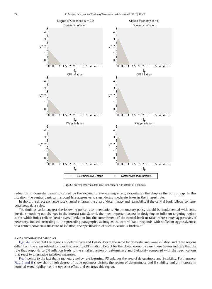
Fig. 2. Contemporaneous data rule: benchmark rule-effects of openness.

22 E. Araújo / International Review of Economics and Finance 45 (2016) 16–32

reduction in domestic demand, caused by the expenditure-switching effect, exacerbates the drop in the output gap. In thissituation, the central bank can respond less aggressively, engendering moderate hikes in the interest rate.

In short, the direct exchange rate channel enlarges the area of determinacy and learnability if the central bank follows contem-poraneous data rules.

The findings so far suggest the following policy recommendations. First, monetary policy should be implemented with someinertia, smoothing out changes in the interest rate. Second, the most important aspect in designing an inflation targeting regimeis not which index reflects better overall inflation but the commitment of the central bank to raise interest rates aggressively ifnecessary. Indeed, according to the preceding paragraphs, as long as the central bank responds with sufficient aggressivenessto a contemporaneous measure of inflation, the specification of such measure is irrelevant.

3.2.2. Forecast-based data rulesFigs. 4–6 show that the regions of determinacy and E-stability are the same for domestic and wage inflation and these regions

differ from the areas related to rules that react to CPI inflation. Except for the closed economy case, these figures indicate that therule that responds to CPI inflation leads to the smallest region of determinacy and E-stability compared with the specificationsthat react to alternative inflation measures.

Fig. 4 points to the fact that a monetary policy rule featuring IRS enlarges the area of determinacy and E-stability. Furthermore,Figs. 5 and 6 show that a high degree of trade openness shrinks the region of determinacy and E-stability and an increase innominal wage rigidity has the opposite effect and enlarges this region.

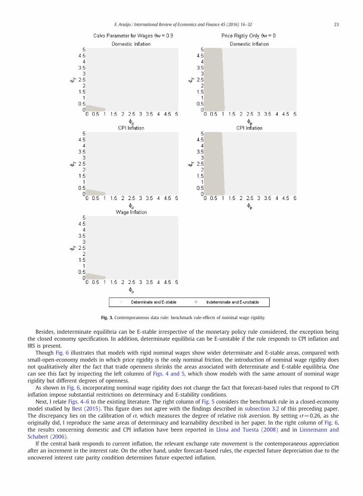
Fig. 3. Contemporaneous data rule: benchmark rule-effects of nominal wage rigidity.

23E. Araújo / International Review of Economics and Finance 45 (2016) 16–32

Besides, indeterminate equilibria can be E-stable irrespective of the monetary policy rule considered, the exception beingthe closed economy specification. In addition, determinate equilibria can be E-unstable if the rule responds to CPI inflation andIRS is present.

Though Fig. 6 illustrates that models with rigid nominal wages show wider determinate and E-stable areas, compared withsmall-open-economy models in which price rigidity is the only nominal friction, the introduction of nominal wage rigidity doesnot qualitatively alter the fact that trade openness shrinks the areas associated with determinate and E-stable equilibria. Onecan see this fact by inspecting the left columns of Figs. 4 and 5, which show models with the same amount of nominal wagerigidity but different degrees of openness.

As shown in Fig. 6, incorporating nominal wage rigidity does not change the fact that forecast-based rules that respond to CPIinflation impose substantial restrictions on determinacy and E-stability conditions.

Next, I relate Figs. 4–6 to the existing literature. The right column of Fig. 5 considers the benchmark rule in a closed-economymodel studied by Best (2015). This figure does not agree with the findings described in subsection 3.2 of this preceding paper.The discrepancy lies on the calibration of σ, which measures the degree of relative risk aversion. By setting σ=0.26, as sheoriginally did, I reproduce the same areas of determinacy and learnability described in her paper. In the right column of Fig. 6,the results concerning domestic and CPI inflation have been reported in Llosa and Tuesta (2008) and in Linnemann andSchabert (2006).

If the central bank responds to current inflation, the relevant exchange rate movement is the contemporaneous appreciationafter an increment in the interest rate. On the other hand, under forecast-based rules, the expected future depreciation due to theuncovered interest rate parity condition determines future expected inflation.

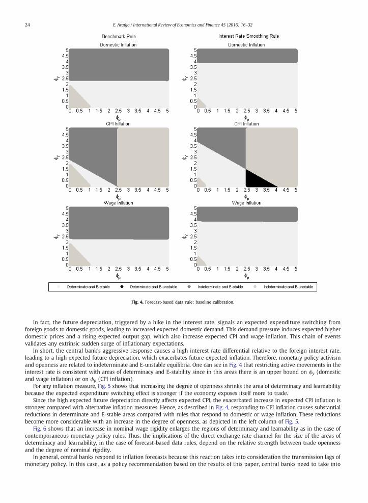
Fig. 4. Forecast-based data rule: baseline calibration.

24 E. Araújo / International Review of Economics and Finance 45 (2016) 16–32

In fact, the future depreciation, triggered by a hike in the interest rate, signals an expected expenditure switching fromforeign goods to domestic goods, leading to increased expected domestic demand. This demand pressure induces expected higherdomestic prices and a rising expected output gap, which also increase expected CPI and wage inflation. This chain of eventsvalidates any extrinsic sudden surge of inflationary expectations.

In short, the central bank's aggressive response causes a high interest rate differential relative to the foreign interest rate,leading to a high expected future depreciation, which exacerbates future expected inflation. Therefore, monetary policy activismand openness are related to indeterminate and E-unstable equilibria. One can see in Fig. 4 that restricting active movements in theinterest rate is consistent with areas of determinacy and E-stability since in this areas there is an upper bound on ϕy (domesticand wage inflation) or on ϕp (CPI inflation).

For any inflation measure, Fig. 5 shows that increasing the degree of openness shrinks the area of determinacy and learnabilitybecause the expected expenditure switching effect is stronger if the economy exposes itself more to trade.

Since the high expected future depreciation directly affects expected CPI, the exacerbated increase in expected CPI inflation isstronger compared with alternative inflation measures. Hence, as described in Fig. 4, responding to CPI inflation causes substantialreductions in determinate and E-stable areas compared with rules that respond to domestic or wage inflation. These reductionsbecome more considerable with an increase in the degree of openness, as depicted in the left column of Fig. 5.

Fig. 6 shows that an increase in nominal wage rigidity enlarges the regions of determinacy and learnability as in the case ofcontemporaneous monetary policy rules. Thus, the implications of the direct exchange rate channel for the size of the areas ofdeterminacy and learnability, in the case of forecast-based data rules, depend on the relative strength between trade opennessand the degree of nominal rigidity.

In general, central banks respond to inflation forecasts because this reaction takes into consideration the transmission lags ofmonetary policy. In this case, as a policy recommendation based on the results of this paper, central banks need to take into

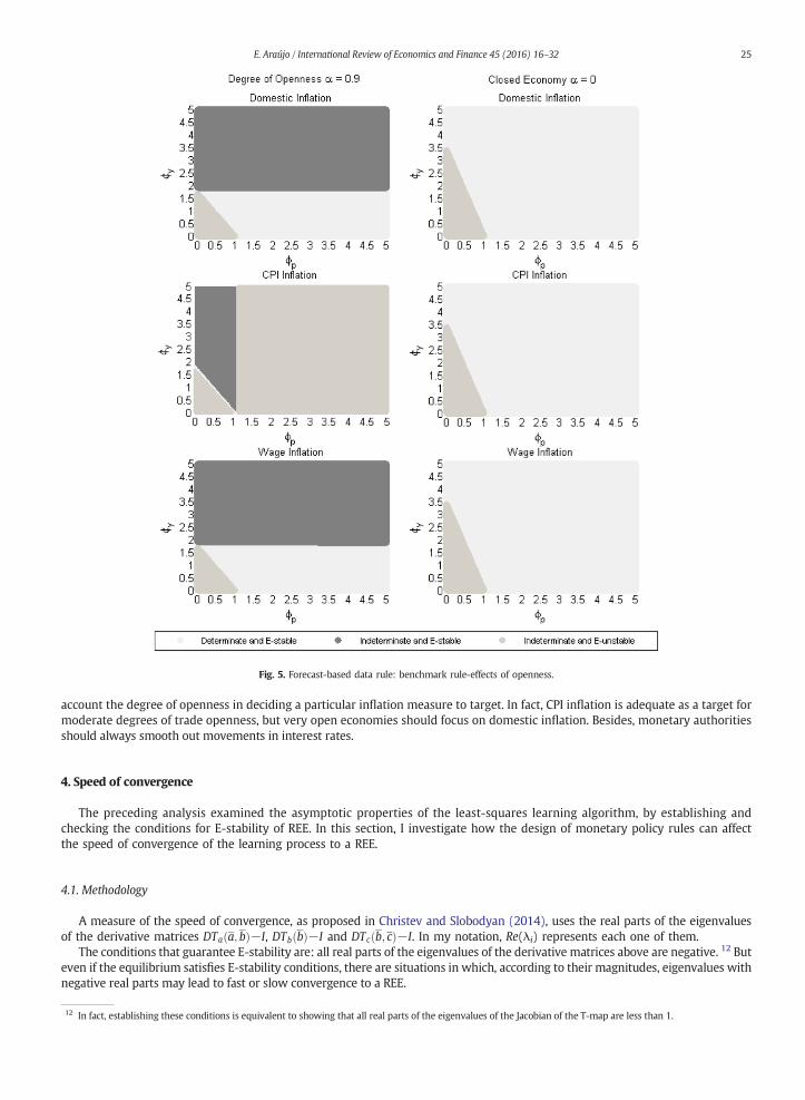
Fig. 5. Forecast-based data rule: benchmark rule-effects of openness.

25E. Araújo / International Review of Economics and Finance 45 (2016) 16–32

account the degree of openness in deciding a particular inflation measure to target. In fact, CPI inflation is adequate as a target formoderate degrees of trade openness, but very open economies should focus on domestic inflation. Besides, monetary authoritiesshould always smooth out movements in interest rates.

4. Speed of convergence

The preceding analysis examined the asymptotic properties of the least-squares learning algorithm, by establishing andchecking the conditions for E-stability of REE. In this section, I investigate how the design of monetary policy rules can affectthe speed of convergence of the learning process to a REE.

4.1. Methodology

A measure of the speed of convergence, as proposed in Christev and Slobodyan (2014), uses the real parts of the eigenvaluesof the derivative matrices DTaða; bÞ−I, DTbðbÞ−I and DTcðb; cÞ−I. In my notation, Re(λi) represents each one of them.

The conditions that guarantee E-stability are: all real parts of the eigenvalues of the derivative matrices above are negative. 12 Buteven if the equilibrium satisfies E-stability conditions, there are situations in which, according to their magnitudes, eigenvalues withnegative real parts may lead to fast or slow convergence to a REE.

12 In fact, establishing these conditions is equivalent to showing that all real parts of the eigenvalues of the Jacobian of the T-map are less than 1.

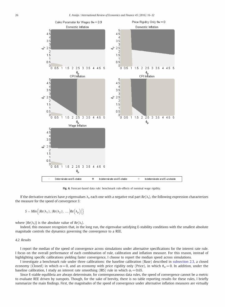
Fig. 6. Forecast-based data rule: benchmark rule-effects of nominal wage rigidity.

26 E. Araújo / International Review of Economics and Finance 45 (2016) 16–32

If the derivative matrices have p eigenvalues λi, each one with a negative real part Re(λi), the following expression characterizesthe measure for the speed of convergence S:

S ¼ Min Re λ1ð Þj j; Re λ2ð Þj j; :::; Re λp

� ���� ���n o

where |Re(λi)| is the absolute value of Re(λi).Indeed, this measure recognizes that, in the long run, the eigenvalue satisfying E-stability conditions with the smallest absolute

magnitude controls the dynamics governing the convergence to a REE.

4.2. Results

I report the median of the speed of convergence across simulations under alternative specifications for the interest rate rule.I focus on the overall performance of each combination of rule, calibration and inflation measure. For this reason, instead ofhighlighting specific calibrations yielding faster convergence, I choose to report the median speed across simulations.

I investigate a benchmark rule under three calibrations: the baseline calibration (Base) described in subsection 2.3, a closedeconomy (Closed) in which α=0, and an economy with price rigidity only (Price), in which θw=0. In addition, under thebaseline calibration, I study an interest rate smoothing (IRS) rule in which ϕr=0.65.

Since E-stable equilibria are always determinate, for contemporaneous data rules, the speed of convergence cannot be a metricto evaluate REE driven by sunspots. Though, for the sake of brevity, there is no table reporting results for these rules, I brieflysummarize the main findings. First, the magnitudes of the speed of convergence under alternative inflation measures are virtually

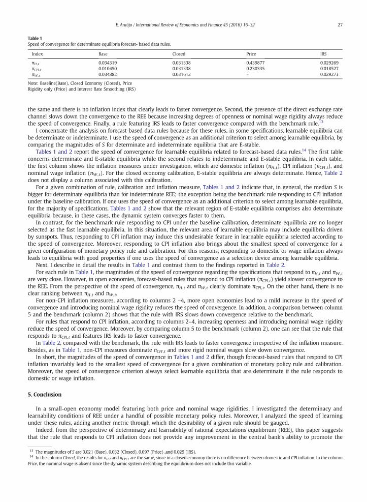
Table 1Speed of convergence for determinate equilibria forecast- based data rules.

Index Base Closed Price IRS

πH ,t 0.034319 0.031338 0.439877 0.029269πCPI ,t 0.010450 0.031338 0.230335 0.018527πW ,t 0.034882 0.031612 – 0.029273

Note: Baseline(Base), Closed Economy (Closed), PriceRigidity only (Price) and Interest Rate Smoothing (IRS)

27E. Araújo / International Review of Economics and Finance 45 (2016) 16–32

the same and there is no inflation index that clearly leads to faster convergence. Second, the presence of the direct exchange ratechannel slows down the convergence to the REE because increasing degrees of openness or nominal wage rigidity always reducethe speed of convergence. Finally, a rule featuring IRS leads to faster convergence compared with the benchmark rule.13

I concentrate the analysis on forecast-based data rules because for these rules, in some specifications, learnable equilibria canbe determinate or indeterminate. I use the speed of convergence as an additional criterion to select among learnable equilibria, bycomparing the magnitudes of S for determinate and indeterminate equilibria that are E-stable.

Tables 1 and 2 report the speed of convergence for learnable equilibria related to forecast-based data rules.14 The first tableconcerns determinate and E-stable equilibria while the second relates to indeterminate and E-stable equilibria. In each table,the first column shows the inflation measures under investigation, which are domestic inflation (πH ,t), CPI inflation (πCPI ,t), andnominal wage inflation (πW ,t). For the closed economy calibration, E-stable equilibria are always determinate. Hence, Table 2does not display a column associated with this calibration.

For a given combination of rule, calibration and inflation measure, Tables 1 and 2 indicate that, in general, the median S isbigger for determinate equilibria than for indeterminate REE; the exception being the benchmark rule responding to CPI inflationunder the baseline calibration. If one uses the speed of convergence as an additional criterion to select among learnable equilibria,for the majority of specifications, Tables 1 and 2 show that the relevant region of E-stable equilibria comprises also determinateequilibria because, in these cases, the dynamic system converges faster to them.

In contrast, for the benchmark rule responding to CPI under the baseline calibration, determinate equilibria are no longerselected as the fast learnable equilibria. In this situation, the relevant area of learnable equilibria may include equilibria drivenby sunspots. Thus, responding to CPI inflation may induce this undesirable feature in learnable equilibria selected according tothe speed of convergence. Moreover, responding to CPI inflation also brings about the smallest speed of convergence for agiven configuration of monetary policy rule and calibration. For this reasons, responding to domestic or wage inflation alwaysleads to equilibria with good properties if one uses the speed of convergence as a selection device among learnable equilibria.

Next, I describe in detail the results in Table 1 and contrast them to the findings reported in Table 2.For each rule in Table 1, the magnitudes of the speed of convergence regarding the specifications that respond to πH ,t and πW ,t

are very close. However, in open economies, forecast-based rules that respond to CPI inflation (πCPI ,t) yield slower convergence tothe REE. From the perspective of the speed of convergence, πH ,t and πW ,t clearly dominate πCPI ,t. On the other hand, there is noclear ranking between πH ,t and πW ,t.

For non-CPI inflation measures, according to columns 2 –4, more open economies lead to a mild increase in the speed ofconvergence and introducing nominal wage rigidity reduces the speed of convergence. In addition, a comparison between column5 and the benchmark (column 2) shows that the rule with IRS slows down convergence relative to the benchmark.

For rules that respond to CPI inflation, according to columns 2–4, increasing openness and introducing nominal wage rigidityreduce the speed of convergence. Moreover, by comparing column 5 to the benchmark (column 2), one can see that the rule thatresponds to πCPI ,t and features IRS leads to faster convergence.

In Table 2, compared with the benchmark, the rule with IRS leads to faster convergence irrespective of the inflation measure.Besides, as in Table 1, non-CPI measures dominate πCPI ,t and more rigid nominal wages slow down convergence.

In short, the magnitudes of the speed of convergence in Tables 1 and 2 differ, though forecast-based rules that respond to CPIinflation invariably lead to the smallest speed of convergence for a given combination of monetary policy rule and calibration.Moreover, the speed of convergence criterion always select learnable equilibria that are determinate if the rule responds todomestic or wage inflation.

5. Conclusion

In a small-open economy model featuring both price and nominal wage rigidities, I investigated the determinacy andlearnability conditions of REE under a handful of possible monetary policy rules. Moreover, I analyzed the speed of learningunder these rules, adding another metric through which the desirability of a given rule should be gauged.

Indeed, from the perspective of determinacy and learnability of rational expectations equilibrium (REE), this paper suggeststhat the rule that responds to CPI inflation does not provide any improvement in the central bank's ability to promote the

13 The magnitudes of S are 0.021 (Base), 0.032 (Closed), 0.097 (Price) ,and 0.025 (IRS).14 In the column Closed, the results for πH,t and πCPI,t are the same, since in a closed economy there is no difference between domestic and CPI inflation. In the columnPrice, the nominal wage is absent since the dynamic system describing the equilibrium does not include this variable.

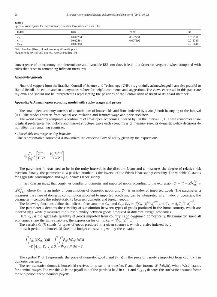
Table 2Speed of convergence for indeterminate equilibria forecast-based data rules.

Index Base Price IRS

πH ,t 0.017234 0.192231 0.018516πCPI ,t 0.012561 0.097692 0.015730πW ,t 0.017318 – 0.018640

Note: Baseline (Base), closed economy (Closed), price.Rigidity only (Price) and Interest Rate Smoothing (IRS).

28 E. Araújo / International Review of Economics and Finance 45 (2016) 16–32

convergence of an economy to a determinate and learnable REE, nor does it lead to a faster convergence when compared withrules that react to contending inflation measures.

Acknowledgments

Financial support from the Brazilian Council of Science and Technology (CNPq) is gratefully acknowledged. I am also grateful toHamid Beladi, the editor, and an anonymous referee for helpful comments and suggestions. The views expressed in this paper aremy own and should not be interpreted as representing the positions of the Central Bank of Brazil or its board members.

Appendix A. A small open economy model with sticky wages and prices

The small open economy consists of a continuum of households and firms indexed by h and j, both belonging to the interval[0,1]. The model abstracts from capital accumulation and features wage and price stickiness.

The world economy comprises a continuum of small open economies indexed by i in the interval [0,1]. These economies shareidentical preferences, technology and market structure. Since each economy is of measure zero, its domestic policy decisions donot affect the remaining countries.

• Households and wage-setting behaviorThe representative household h maximizes the expected flow of utility given by the expression:

E0X∞t¼0

βt C1−σt

1−σ−

Nt hð Þ1þφ

1þ φ

" #

The parameter β, restricted to be in the unity interval, is the discount factor and σ measures the degree of relative riskaversion. Finally, the parameter φ, a positive number, is the inverse of the Frisch labor supply elasticity. The variable Ct standsfor aggregate consumption and Nt(h) denotes labor supply.

In fact, Ct is an index that combines bundles of domestic and imported goods according to the expression Ct ¼ ½ð1−αÞ1ηCη−1η

H;t þ

α1ηC

η−1ηF;t �, where CH , t is an index of consumption of domestic goods and CF , t is an index of imported goods. The parameter α

measures the share of domestic consumption allocated to imported goods and can be interpreted as an index of openness; theparameter η controls the substitutability between domestic and foreign goods.

The following functions define the indices of consumption CH ,t and CF ,t: CH;t ¼ ð∫10CH;tð jÞε−1ε djÞ

εε−1 and C F;t ¼ ð∫10Ci;t

γ−1γ diÞ

γ−1γ.

The parameter ε denotes the elasticity of substitution between types of goods produced in the home country, which areindexed by j, while γ measures the substitutability between goods produced in different foreign economies.

Here, Ci , t is the aggregate quantity of goods imported from country i and consumed domestically. By symmetry, since alleconomies share the same structure, the expression for Ci ,t is: Ci;t ¼ ð∫10Ci;tð jÞ

ε−1ε djÞ

εε−1

.The variable Ci ,t(j) stands for types of goods produced in a given country i, which are also indexed by j.In each period the household faces the budget constraint given by the equation:

Z 1

0PH;t jð ÞCH;t jð Þdjþ

Z 1

0

Z 1

0Pi;t jð ÞCi;t jð Þdjdi

þEt ψt;tþ1Dtþ1

h i≤ Dt þWt hð ÞNt hð Þ þ Tt

The symbol PH , t(j) represents the price of domestic good j and Pi , t(j) is the price of variety j imported from country i indomestic currency.

The representative domestic household receives lump-sum net transfers Tt and labor income Wt(h)Nt(h), where Wt(h) standsfor nominal wages. The variable Dt is the payoff in t of the portfolio held in t−1 and Ψt ,t+1 denotes the stochastic discount factorfor one-period ahead nominal payoffs.

29E. Araújo / International Review of Economics and Finance 45 (2016) 16–32

From the optimal allocation of any given consumption expenditure within each category of goods, I get the followingprice indices:

Pt ¼ 1− αð ÞP1−ηH;t þ αP1−η

F;t

h i 11−η

PH;t ¼Z 1

0PH;t jð Þ1−εdj

� � 11−ε

P F;t ¼Z 1

0P1−γi;t di

� �1

1− γ

Pi;t ¼Z 1

0Pi;t jð Þ1−εdj

� � 11−ε

Based on the price indices, I can rewrite the budget constraint as follows.

PtCt þ Et Ψt;tþ1Dtþ1

h i≤ Dt þWt hð ÞNt hð Þ þ Tt

As in Gal and Monacelli (2005), the assumption of complete markets implies the following risk-sharing condition: Ct ¼ Q1σi;tCi;t,

where Qi ,t stands for the bilateral real exchange rate between countries i and H.The household h chooses consumption Ct, labor Nt(h) and bonds Dt in order to maximize the expected flow of utility subject to

the budget constraint. According to Erceg et al. (2000), there is also a wage-setting decision stage in which each individual h maychoose Wt(h) optimally.

Next, I discuss the wage decision. The representative household h supplies differentiated labor inputs Nt(j,h) for the

production of each variety j. Indeed, total labor supplied and the aggregate wage index are given by NtðhÞ ¼ ∫10Ntð j; hÞdj and Wt ¼

ð∫10WtðhÞ1−εw

dhÞ1

1−εw.

Following Erceg et al. (2000), in each period, only a fraction (1−θw) of households can resetwages optimally in order tomaximizethe expected flow of utility. The log-linear rule that approximates the optimal wage-setting strategy is the following:

wt ¼1−βθw1þ φεw

X∞k¼0

βθwð Þk

Et μw þmrstþk þ φεwwtþk þ ptþk

The symbol wt denotes the log of the newly set nominal wageWt, the log of the steady-state wage mark-up is μw ¼ logð εwεw−1Þ,

mrst stands for the marginal rate of substitution between consumption and labor in log, wt is the log of nominal wages and ptrepresents the log of the consumer price index.

Under the assumed wage-setting scheme, the aggregate wage index evolves according to the equation:

Wt ¼ ½θwW1−εwt−1 þ ð1− θwÞðWtÞ1−εw �

11−εw

:

The log-linearization around the steady state yields the following formula for the wage inflation: πW ,t=(1−θw)( wt−wt−1Þ.After some algebra, the combination of the expressions describing the optimal wage-setting strategy and the evolution of the

aggregate wage index results in Eq. (3) of the main text.

• Firms and price-setting behaviorThe production function Yt(j)=AtNt(j) describes the technology for firm j. The variables Yt(j) and Nt(j) represent output and anindex of labor input used by firm j. The technology shock is At, with at= log(At) following a first order autoregressive process.

The expression Ntð jÞ ¼ ð∫10Ntð j;hÞεw−1εw dhÞ

εwεw−1

defines the index of labor input Nt(j) and the aggregate output is given by Yt ¼

ð∫10Ytð jÞε−1ε djÞ

εε−1

, where εw is the elasticity of substitution between labor varieties and ε is the elasticity of substitution acrossdifferent good varieties.Firms operate in a monopolistic competitive market and set prices in staggered fashion using the scheme proposed by Calvo(1983), in which only a fraction (1−θph) of firms can adjust prices. In this context, in each period, these firms reset their pricesto maximize expected profits. The following log-linear rule approximates the optimal price-setting strategy:

pH;t ¼ μph þ 1−βθph� �X∞

k¼0

βθph� �

Et mctþk þ pH;tþk

h i

The variable pH;t represents the newly set domestic prices PH;t in log, μph ¼ logð εε−1Þ is the log of the steady-state markup, mct

stands for the log of real marginal costs, and pH ,t denotes the log of the domestic price index PH ,t.Real marginal costs in log scale are given bymct=−v+wt−pH ,t−at, where wt is the log of nominal wages and v= log(1−τ),

with τ representing an employment subsidy. This subsidy neutralizes the distortion due to firms' market power, leaving the economywith nominal stickiness as the only effective distortion. Hence, the flexible price equilibrium is efficient. This equilibrium defines thenatural level of macroeconomic variables.

30 E. Araújo / International Review of Economics and Finance 45 (2016) 16–32

Under the assumed price-setting behavior, the equation below describes the dynamics of the domestic price index:

PH;t ¼ θphP1−εH;t−1 þ 1− θph

� �PH;t

� �1−ε� � 1

1−ε:

The log-linearization around the steady state yields the formula involving domestic inflation: πH ,t=(1−θph)( pH;t−pH;t−1Þ.After some algebra, the expressions describing the optimal price-setting strategy and the dynamics of the domestic price index

lead to the new Keynesian Phillips curve as stated by Eq. (2) of the main text.

• Market clearing conditions and monetary policyThe domestic good market clearing condition yields the following expression:

YH;t jð Þ ¼ CH;t jð Þ þ ∫10 CiH;t jð Þdi

After some algebra involving the definitions of the demand functions for CH ,t(j) and CH ,ti (j), I have

YH;t jð Þ ¼ PH;t jð ÞPH;t

!−ε

1−αð Þ PH;t

Pt

� �−ηCt þ α∫10

PH;t

ΞitPiF;t

!−γ PiF;t

Pit

!−η

Citdi

" #

The variable CH ,ti (j) denotes the demand from country i of good j produced in the home economy, Ξit is the nominal exchange

rate, and PF ,ti is the price index for goods imported by country i expressed in its own currency. Lastly, Pti is the consumer price

index for households living in country i.Using the definition of aggregate output Yt ¼ ð∫10 Ytð jÞ

ε−1ε djÞ

εε−1, I get the following expression:

Yt ¼PH;t

Pt

� �−ηCt 1− αð Þ þ α½ �∫10 SitSi;t

� �γ−ηQη−1

σi;t di

The effective terms of trade for country i is Sit ¼ΞitP

iF;t

PH;tand Si;t ¼ Pi;t

PH;tdenotes the bilateral terms of trade between country i and

the domestic economy H . Finally, Qi;t ¼ EitPit

Ptrepresents the bilateral real exchange rate between countries i and H.

The labor market clearing condition is: Nt= ∫01 Nt(j)dj= ∫01 Nt(h)dh.To close the model, I assume that the central bank follows the interest rate rules described in subsection 2.2 of the main text.

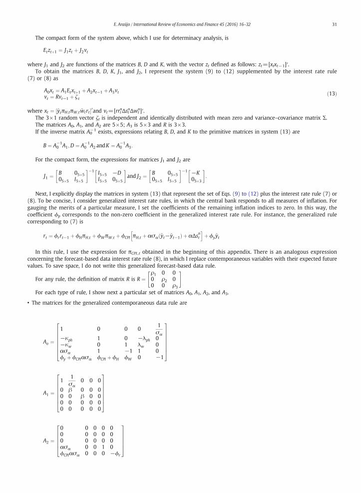
Appendix B. The matrix representation of the parsimonious system

Concerning the private sector equilibrium conditions, I reduce the original system in subsection 2.1 to a smaller one with fiveendogenous variables: ~yt , πH ,t, πW ,t, ~wt , and rt. To accomplish this reduction, I use Eq. (6) to solve for st and Eq. (5) to get thefollowing expression for CPI inflation: πCPI;t ¼ πH;t þ ασαð~yt−~yt−1Þ þ αΔsnt , where Δstn=σα(Δytn−Δyt⁎). After substituting outπCPI ,t in Eq. (4), this expression becomes Eq. (12). The parsimonious system comprises the following equations:

~yt ¼ Et ~yt þ 1ð Þ− 1σα

rt − Et πH;tþ1

� �h iþ 1σα

rrnt ð9Þ

πH;t ¼ βEt πH;tþ1

� �þ κph~yt þ λph ~wt ð10Þ

πW;t ¼ βEt πW;tþ1

� �þ κw~yt − λw ~wt ð11Þ

~wt ¼ ~wt−1 þ πW;t − πH;t − ασα ~yt − ~yt−1ð Þ−αΔsny −Δwny ð12Þ

The last equation that closes the system is one of the interest rate rules discussed in subsection 2.2.Subsection 3.1 considers the following system of linear stochastic difference equations:

xt ¼ BEtxtþ1 þ Dxt−1 þ Kvt

vt ¼ Rvt−1 þ ζ t

where xt is a m×1 vector of endogenous variables and vt is a k×1 vector of exogenous disturbances.

31E. Araújo / International Review of Economics and Finance 45 (2016) 16–32

The compact form of the system above, which I use for determinacy analysis, is

Etztþ1 ¼ J1zt þ J2vt

where J1 and J2 are functions of the matrices B, D and K, with the vector zt defined as follows: zt=[xtxt−1]′.To obtain the matrices B, D, K, J1, and J2, I represent the system (9) to (12) supplemented by the interest rate rule

(7) or (8) as

A0xt ¼ A1Etxtþ1 þ A2xt−1 þ A3vtvt ¼ Rvt−1 þ ζ t

ð13Þ

where xt ¼ ½~ytπH;tπW;t ~wtrt �0and vt=[rrtnΔstnΔwtn]′.

The 3×1 random vector ζt is independent and identically distributed with mean zero and variance–covariance matrix Σ.The matrices A0, A1, and A2 are 5×5; A3 is 5×3 and R is 3×3.If the inverse matrix A0

−1 exists, expressions relating B, D, and K to the primitive matrices in system (13) are

B ¼ A−10 A1;D ¼ A−1

0 A2 andK ¼ A−10 A3:

For the compact form, the expressions for matrices J1 and J2 are

J1 ¼ B 05�505�5 I5�5

� �−1 I5�5 −DI5�5 05�5

� �and J2 ¼ B 05�5

05�5 I5�5

� �−1 −K05�3

� �:

Next, I explicitly display the matrices in system (13) that represent the set of Eqs. (9) to (12) plus the interest rate rule (7) or(8). To be concise, I consider generalized interest rate rules, in which the central bank responds to all measures of inflation. Forgauging the merits of a particular measure, I set the coefficients of the remaining inflation indices to zero. In this way, thecoefficient ϕp corresponds to the non-zero coefficient in the generalized interest rate rule. For instance, the generalized rulecorresponding to (7) is

rt ¼ ϕrrt−1 þ ϕHπH;t þ ϕWπW;t þ ϕCPI πH;t þ ασα ~yt−~yt−1ð Þ þ αΔsnth i

þ ϕy~yt

In this rule, I use the expression for πCPI , t obtained in the beginning of this appendix. There is an analogous expressionconcerning the forecast-based data interest rate rule (8), in which I replace contemporaneous variables with their expected futurevalues. To save space, I do not write this generalized forecast-based data rule.

For any rule, the definition of matrix R is R ¼"ρ1 0 00 ρ2 00 0 ρ3

#

For each type of rule, I show next a particular set of matrices A0, A1, A2, and A3.

• The matrices for the generalized contemporaneous data rule are

Ao ¼

1 0 0 01σα

−κph 1 0 −λph 0−κw 0 1 λw 0ασα 1 −1 1 0ϕy þ ϕCPIασα ϕCPI þ ϕH ϕW 0 −1

26666664

37777775

A1 ¼

11σα

0 0 0

0 β 0 0 00 0 β 0 00 0 0 0 00 0 0 0 0

26666664

37777775

A2 ¼

0 0 0 0 00 0 0 0 00 0 0 0 0ασα 0 0 1 0ϕCPIασα 0 0 0 −ϕr

266664

377775

32 E. Araújo / International Review of Economics and Finance 45 (2016) 16–32

1σα

0 0266

377

A3 ¼ 0 0 00 0 00 −α −10 −ϕCPIα 0

6666477775

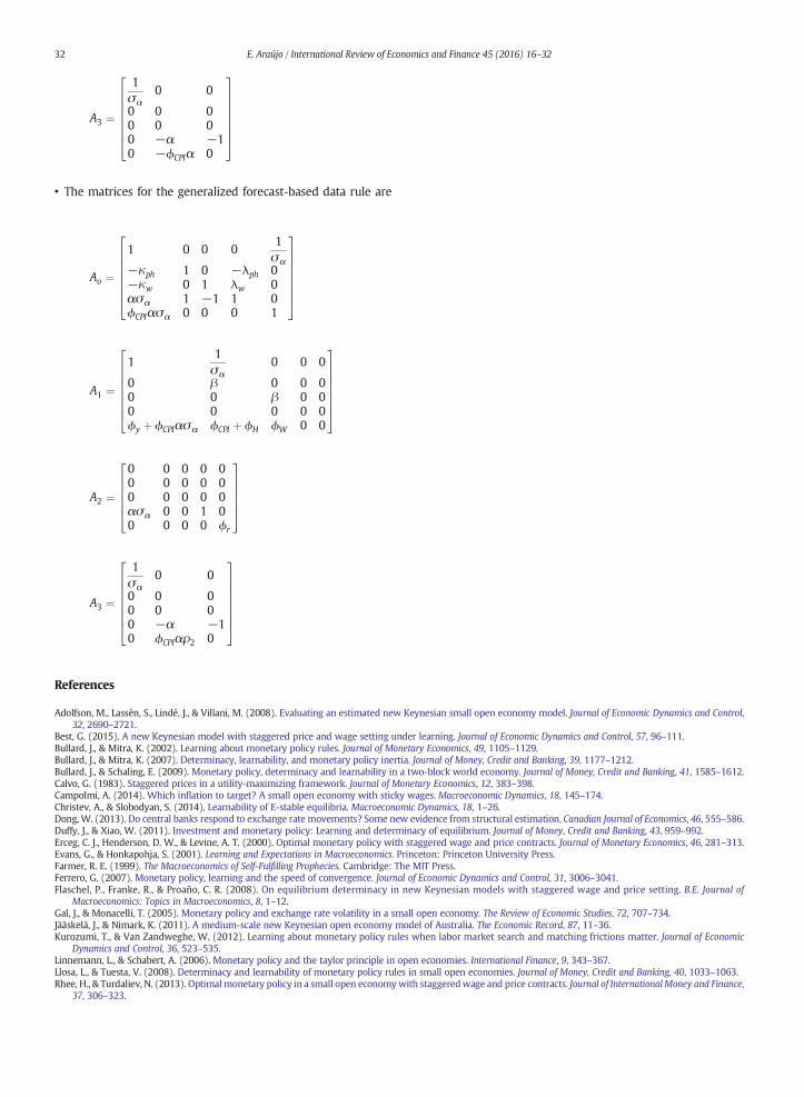
• The matrices for the generalized forecast-based data rule are

Ao ¼

1 0 0 01σα

−κph 1 0 −λph 0−κw 0 1 λw 0ασα 1 −1 1 0ϕCPIασα 0 0 0 1

26666664

37777775

A1 ¼

11σα

0 0 0

0 β 0 0 00 0 β 0 00 0 0 0 0ϕy þ ϕCPIασα ϕCPI þ ϕH ϕW 0 0

26666664

37777775

A2 ¼

0 0 0 0 00 0 0 0 00 0 0 0 0ασα 0 0 1 00 0 0 0 ϕr

266664

377775

A3 ¼

1σα

0 0

0 0 00 0 00 −α −10 ϕCPIαρ2 0

26666664

37777775

References

Adolfson, M., Lassén, S., Lindé, J., & Villani, M. (2008). Evaluating an estimated new Keynesian small open economy model. Journal of Economic Dynamics and Control,32, 2690–2721.

Best, G. (2015). A new Keynesian model with staggered price and wage setting under learning. Journal of Economic Dynamics and Control, 57, 96–111.Bullard, J., & Mitra, K. (2002). Learning about monetary policy rules. Journal of Monetary Economics, 49, 1105–1129.Bullard, J., & Mitra, K. (2007). Determinacy, learnability, and monetary policy inertia. Journal of Money, Credit and Banking, 39, 1177–1212.Bullard, J., & Schaling, E. (2009). Monetary policy, determinacy and learnability in a two-block world economy. Journal of Money, Credit and Banking, 41, 1585–1612.Calvo, G. (1983). Staggered prices in a utility-maximizing framework. Journal of Monetary Economics, 12, 383–398.Campolmi, A. (2014). Which inflation to target? A small open economy with sticky wages. Macroeconomic Dynamics, 18, 145–174.Christev, A., & Slobodyan, S. (2014). Learnability of E-stable equilibria. Macroeconomic Dynamics, 18, 1–26.Dong, W. (2013). Do central banks respond to exchange rate movements? Some new evidence from structural estimation. Canadian Journal of Economics, 46, 555–586.Duffy, J., & Xiao, W. (2011). Investment and monetary policy: Learning and determinacy of equilibrium. Journal of Money, Credit and Banking, 43, 959–992.Erceg, C. J., Henderson, D. W., & Levine, A. T. (2000). Optimal monetary policy with staggered wage and price contracts. Journal of Monetary Economics, 46, 281–313.Evans, G., & Honkapohja, S. (2001). Learning and Expectations in Macroeconomics. Princeton: Princeton University Press.Farmer, R. E. (1999). The Macroeconomics of Self-Fulfilling Prophecies. Cambridge: The MIT Press.Ferrero, G. (2007). Monetary policy, learning and the speed of convergence. Journal of Economic Dynamics and Control, 31, 3006–3041.Flaschel, P., Franke, R., & Proaño, C. R. (2008). On equilibrium determinacy in new Keynesian models with staggered wage and price setting. B.E. Journal of

Macroeconomics: Topics in Macroeconomics, 8, 1–12.Gal, J., & Monacelli, T. (2005). Monetary policy and exchange rate volatility in a small open economy. The Review of Economic Studies, 72, 707–734.Jääskelä, J., & Nimark, K. (2011). A medium-scale new Keynesian open economy model of Australia. The Economic Record, 87, 11–36.Kurozumi, T., & Van Zandweghe, W. (2012). Learning about monetary policy rules when labor market search and matching frictions matter. Journal of Economic

Dynamics and Control, 36, 523–535.Linnemann, L., & Schabert, A. (2006). Monetary policy and the taylor principle in open economies. International Finance, 9, 343–367.Llosa, L., & Tuesta, V. (2008). Determinacy and learnability of monetary policy rules in small open economies. Journal of Money, Credit and Banking, 40, 1033–1063.Rhee, H., & Turdaliev, N. (2013). Optimalmonetary policy in a small open economywith staggeredwage and price contracts. Journal of International Money and Finance,

37, 306–323.