Detection Techniques for Data-Level Spoofing inGPS-Based Phasor Measurement Units

Fu Zhu

A Thesis

in

The Department

of

Engineering and Computer Science

Presented in Partial Fulfillment of the Requirements

for the Degree of

Master of Applied Science (Electrical and Computer Engineering) at

Concordia University

Montreal, Quebec, Canada

November 2016

c© Fu Zhu, 2016

. Amr YoussefDrSupervisor

ScienceComputerandEngineeringofacultyFDeanAsif,Amir

2016

ScienceComputerandEngineeringofDepartmentChairAsif,Amir.Dr

byedvAppro

HamoudaalaaWDrSupervisor

OneExaminerofName.DrExaminer

ExaminerExternalofName.DrExaminerExternal

ChairtheofName.DrChair

Committee:ExaminingFinalthebySigned

qualityandoriginalitytospect

re-withstandardsdacceptethemeetsandersityvUnithisofgulationsrethewithcomplies

Engineering)Computerand(ElectricalScienceppliedAofMaster

ofgreedetheforrequirementstheoffulfillmentpartialinsubmittedand

UnitsementMeasursor

Pha-GPS-BasedinSpoofingelvData-LeorfechniquesTDetectionEntitled:

ZhuFuBy:

preparedthesisthethatcertifytoisThis

StudiesGraduateofSchool

YTISREVINUAIDROCNOC

Abstract

Detection Techniques for Data-Level Spoofing in GPS-Based PhasorMeasurement Units

Fu Zhu

The increasing complexity of todays power system aggravated the stability and real-

time issues. Wide-area monitoring system (WAMS) provides a dynamic coverage which

allows real-time monitoring of critical knows of power systems. Phasor measurement

units (PMUs) are being used in WAMS to provide a wide area system view and increase

the system stability. A PMU is a sensor that measures the three-phase analog voltage,

current and frequency and uploads the phasor information to the Phasor Data Concentrator

(PDC) at a rate of 30 to 60 observations per second. Typically, PMUs utilize a Global

Positioning System (GPS) reference source to provide the required synchronization across

wide geographical areas. On the other hand, civil GPS receivers are vulnerable to a number

of different attacks such as jamming and spoofing, which can lead to inaccurate PMU

measurements and consequently compromise the state estimation in the electric power grid.

In this thesis, we propose three countermeasures against GPS spoofing attacks on

PMUs from three layers in the WAMS. In particular, we utilize the fact that in GPS-based

PMUs, unlike most of the GPS applications, the position of the PMU receivers are already

fixed and known. Our first technique employs an algorithm that accurately predicts the

number of theoretically visible GPS satellites from a given position on earth. If the GPS

receiver detects satellites which should not be visible at that time, this signifies a spoofing

attempt. The second technique is an anomaly-based detection method which assumes that

iii

the statistics of malicious errors in GPS time solutions are unlikely to be consistent with

the expected statistics of the typical receiver clock. We also propose a model which can be

used to analyze the phasor data uploaded from two PMUs to the Phasor Data Concentrator.

The relative phase angle difference (RPAD) is used in our algorithm to detect the spoofing

attack. The algorithm uses Fast Fourier Transform to analyze the RPAD between two

PMUs. We study the behavior of the low frequency component in the FFT result of the

RPAD between that two PMUs to detect the spoofing attacks. The effectiveness of the

proposed techniques is confirmed by simulations.

iv

Acknowledgments

First of all, I would like to thank my supervisors Dr. Amr Youssef and Dr. Walaa

Hamouda for their patient guidance and continuous support throughout my Master’s study

career.

Furthermore, I would like to express special thanks to my parents, Mr.Xinping Zhu

and Mrs. Liping Liu for their continuous love and support. I would also like to thank my

immediate family members, including my uncle Dr. Xianping Liu, my aunt Mrs. Meiling

Yao, my grandma Mrs. Duoyun Zeng for always being there for me.

Last, but not least, I would like to thank my colleagues at Concordia University,

specifically, Anahid Attarkashan, Abdelmohsen Ali, Mahmoud Elsaadany, Oana Neagu,

Katerina Dimogiorgi, Shiwen Zhu, Ce Shi, Haowei song, Wentao Xu, Rusong Miao,

Hongyu Zhang, and Jiyuan Guo for making my time at the university and in Montreal

pleasurable and memorable.

v

Contents

List of Figures viii

List of Tables x

1 Introduction 1

1.1 Overview . . . . . . . . . . . . . . . . . . . . . . . . . . . . . . . . . . . 1

1.2 Motivation . . . . . . . . . . . . . . . . . . . . . . . . . . . . . . . . . . . 2

1.3 Objective . . . . . . . . . . . . . . . . . . . . . . . . . . . . . . . . . . . 4

1.4 Contribution . . . . . . . . . . . . . . . . . . . . . . . . . . . . . . . . . . 4

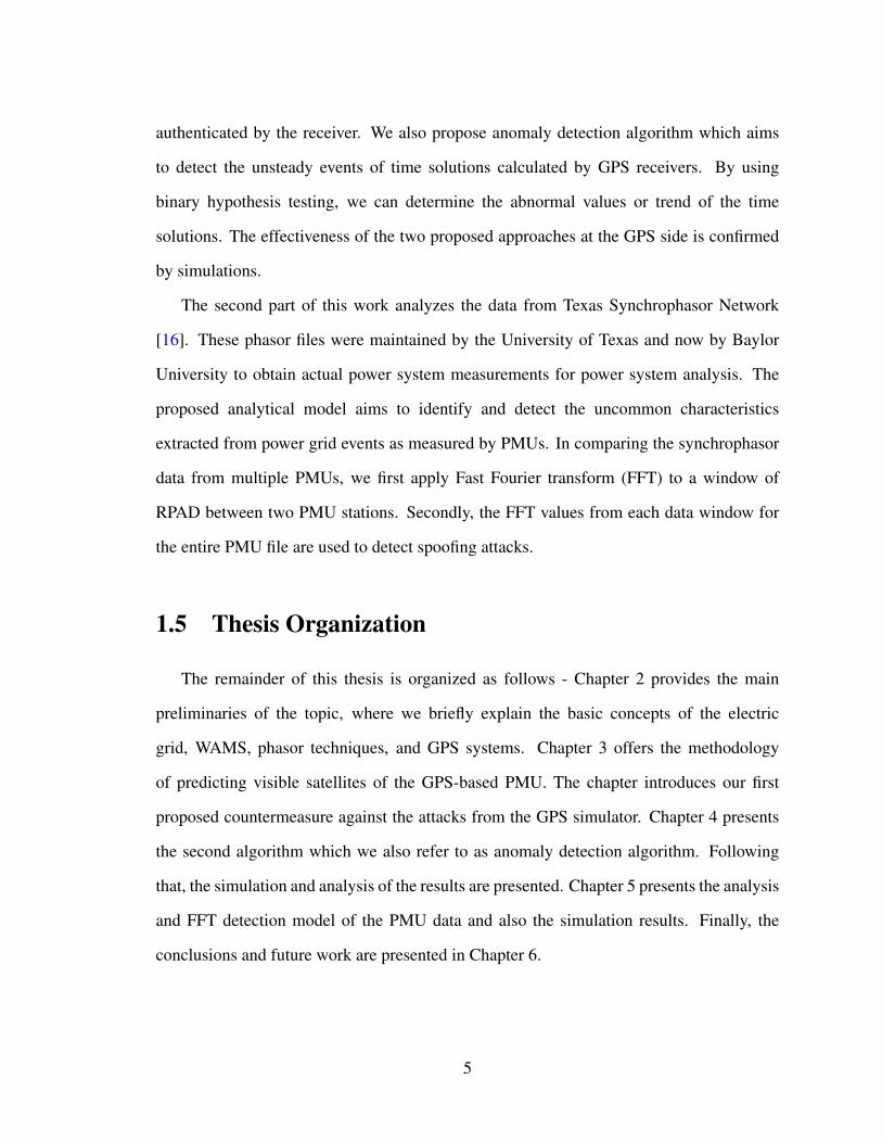
1.5 Thesis Organization . . . . . . . . . . . . . . . . . . . . . . . . . . . . . . 5

2 Preliminaries 6

2.1 Smart Grid . . . . . . . . . . . . . . . . . . . . . . . . . . . . . . . . . . 6

2.1.1 Development of power grid . . . . . . . . . . . . . . . . . . . . . 6

2.1.2 Smart grid technologies . . . . . . . . . . . . . . . . . . . . . . . 9

2.2 Wide-Area Measurement System . . . . . . . . . . . . . . . . . . . . . . . 17

2.2.1 WAMS definition and structure . . . . . . . . . . . . . . . . . . . 17

2.2.2 Phasor techniques . . . . . . . . . . . . . . . . . . . . . . . . . . . 18

2.3 GPS Systems . . . . . . . . . . . . . . . . . . . . . . . . . . . . . . . . . 20

2.3.1 GPS signal components . . . . . . . . . . . . . . . . . . . . . . . 21

2.3.2 GPS receiver position basics . . . . . . . . . . . . . . . . . . . . . 23

vi

i xof AcronymsList

2.3.3 Attacks on GPS . . . . . . . . . . . . . . . . . . . . . . . . . . . . 24

3 Predicting Visible Satellites 26

3.1 Motivation . . . . . . . . . . . . . . . . . . . . . . . . . . . . . . . . . . . 26

3.2 Methodology . . . . . . . . . . . . . . . . . . . . . . . . . . . . . . . . . 28

3.3 Simulation Results . . . . . . . . . . . . . . . . . . . . . . . . . . . . . . 34

3.4 Counclusion . . . . . . . . . . . . . . . . . . . . . . . . . . . . . . . . . . 36

4 Anomaly Detection of Data-Level GPS Spoofing 38

4.1 GPS-PPS Stochastic Error Analysis . . . . . . . . . . . . . . . . . . . . . 38

4.2 Models of Attacks . . . . . . . . . . . . . . . . . . . . . . . . . . . . . . . 40

4.3 Proposed Anomaly Detection Scheme . . . . . . . . . . . . . . . . . . . . 42

4.4 Simulation Results . . . . . . . . . . . . . . . . . . . . . . . . . . . . . . 47

4.5 Conclusions . . . . . . . . . . . . . . . . . . . . . . . . . . . . . . . . . . 49

5 FFT-Dased Detection 50

5.1 Background of Synchrophasor Networks . . . . . . . . . . . . . . . . . . . 50

5.1.1 Phasor measurement unit . . . . . . . . . . . . . . . . . . . . . . . 50

5.1.2 Synchrophasor and PMU data . . . . . . . . . . . . . . . . . . . . 51

5.2 Proposed FFT-based Detection Algorithm . . . . . . . . . . . . . . . . . . 53

5.2.1 Relative phase angle difference . . . . . . . . . . . . . . . . . . . 53

5.2.2 FFT-based detection algorithm . . . . . . . . . . . . . . . . . . . . 55

5.2.3 Simulation Results . . . . . . . . . . . . . . . . . . . . . . . . . . 57

5.3 Conclusion . . . . . . . . . . . . . . . . . . . . . . . . . . . . . . . . . . 60

6 Conclusions and Future Work 62

Bibliography 64

vii

List of Figures

Figure 2.1 Traditional power grid [17] . . . . . . . . . . . . . . . . . . . . . . 7

Figure 2.2 Structure of smart grid [17] . . . . . . . . . . . . . . . . . . . . . . 8

Figure 2.3 Technology of smart grid [24] . . . . . . . . . . . . . . . . . . . . . 10

Figure 2.4 Layers and components of WAMC system [26] . . . . . . . . . . . 10

Figure 2.5 Smart grid communication infrastructures [27] . . . . . . . . . . . . 11

Figure 2.6 Structure and main components of a DMS [29] . . . . . . . . . . . . 14

Figure 2.7 General WAMS structure [30] . . . . . . . . . . . . . . . . . . . . . 18

Figure 2.8 Sinusoidal waveform and phasor representation [31] . . . . . . . . . 19

Figure 2.9 Three core segments of a Global Positioning System [32]. . . . . . . 20

Figure 2.10 Modulation of GPS signal [33] . . . . . . . . . . . . . . . . . . . . 22

Figure 3.1 Block diagram of GPS receiver [37] . . . . . . . . . . . . . . . . . 27

Figure 3.2 Description of SV position from orbital parameters [39] . . . . . . . 29

Figure 3.3 Visible satellites from a fixed elevation angle . . . . . . . . . . . . . 34

Figure 3.4 Prediction of visible satellitesl . . . . . . . . . . . . . . . . . . . . 35

Figure 3.5 Prediction of visible satellites . . . . . . . . . . . . . . . . . . . . . 35

Figure 4.1 Example of Scaling attack, ramp attack, and random attack . . . . . 41

Figure 4.2 Hypothesis testing of anomaly detection 1 . . . . . . . . . . . . . . 43

Figure 4.3 Pre-attacked Ratio value . . . . . . . . . . . . . . . . . . . . . . . . 44

Figure 4.4 Spoofed Ratio value . . . . . . . . . . . . . . . . . . . . . . . . . . 45

Figure 4.5 Hypothesis testing of the anomaly detection part2 . . . . . . . . . . 45

viii

Figure 4.6 Flow chart of anomaly detection algorithm . . . . . . . . . . . . . . 46

Figure 4.7 ROC curve of detect the scaling attack . . . . . . . . . . . . . . . . 48

Figure 4.8 Detection time of anomaly detection . . . . . . . . . . . . . . . . . 48

Figure 5.1 Block diagram of a PMU [13] . . . . . . . . . . . . . . . . . . . . . 51

Figure 5.2 Map of Texas Synchrophasor Network [12] . . . . . . . . . . . . . 52

Figure 5.3 Example of PMU data format [12] . . . . . . . . . . . . . . . . . . 53

Figure 5.4 Raw PMU phase data . . . . . . . . . . . . . . . . . . . . . . . . . 54

Figure 5.5 Raw PMU phase angle and unwrapped curve . . . . . . . . . . . . . 54

Figure 5.6 RPAD between two PMU stations . . . . . . . . . . . . . . . . . . 55

Figure 5.7 sliding window . . . . . . . . . . . . . . . . . . . . . . . . . . . . 56

Figure 5.8 FFT of RPAD between two stations . . . . . . . . . . . . . . . . . . 56

Figure 5.9 FFT results after spoofing attack . . . . . . . . . . . . . . . . . . . 57

Figure 5.10 pdf of first non-zero low frequency component of the RPAD signal . 58

Figure 5.11 Flow chart of the detection procedure . . . . . . . . . . . . . . . . . 59

Figure 5.12 Trend of low frequency changes during attack . . . . . . . . . . . . 60

Figure 5.13 False alarm rate of detection algorithm . . . . . . . . . . . . . . . . 60

ix

List of Tables

Table 1.1 Traditional countermeasures and limitations . . . . . . . . . . . . . . 3

Table 2.1 Smart grid technologies [24] . . . . . . . . . . . . . . . . . . . . . . 16

Table 2.2 Attack on GPS receiver . . . . . . . . . . . . . . . . . . . . . . . . . 25

x

List of Acronyms

AMI Advanced Metering Infrastructure

ATC Available Transmission Capability

BANs Business Area Networks

BAU Business As Usual

BPA BonnevillePower Administration

C/A Coarse/Acquisition

DGs Distributed Generations

DLR Dynamic Line Rating

DMS

DOE Department of Energy

ECEF Earth Centered Earth Fixed

EMS

EPRI Electric Power Research Institute

FA CTS Flexible Alternating Current Transmission System

FFT Fast Fourier Transform

GLON ASS Russian Global Navigation Satellite System

GNSS GlobalNavigation Satellite System

GPS Global Positioning System

HANs Home Area Networks

HTS High-Temperature Superconductors

HVDC High Voltage DC

IF Intermediate Frequency

IGS International GNSS Service

IP Internet Protocol

xi

Distribution System Mangement

Energy System Management

MCS Master Control Station

MGCC Micro-Grid Central Control

NANs Neighborhood Area Networks

PCC Point of Common Coupling

PDC Phasor Data Concentrator

PMUs PhasorMeasurement Units

PPS Pulse-Per-Second

PPS Precision Positioning Code

RF Radio Frequency

RPAD Relative Phase Angle Difference

SCAD A SupervisoryControl and Data Acquisition

SG Smart Grid

SPS Standard Positioning Code

SV Satellite Vehicle

TVE Total Vector Error

W AMC Monitoringand Control

W AMS Wide-Area Measurement Systems

xii

Chapter 1

Introduction

In this chapter, we provide a brief summary of our research work. We start by presenting

some background of the topic and the motivation behind the proposed work. Next, we

review the purpose and major findings of our research. The organization of the thesis is

described at the end of this chapter.

1.1 Overview

Electricity is the groundwork for the whole world’s economic development. Since the

creation of the world’s first power system at Godalming in England [1], the electricity

industry has shown a great advancement. The electric system consists of three parts:

power generation, power transmission from the generator centers to the substations, and

the distribution system.

The traditional power grid is based on a structure of one-way flow of electricity, a

centralized, bulk generation, and unidirectional transmission and distribution systems. The

dispatching of the traditional power system could not meet the need of higher renewable

energy penetration. Recently, new technologies are offering new grid capabilities, and they

are less expensive and more suitable for clean energy sources. They also provide better

1

response times for the consumers when power outage occurs.

A Smart Grid (SG), regarded as the next generation power grid, uses two-way flow

of electricity and information to create a widely distributed automated energy delivery

network [2]. The SG system uses sensors, monitoring, communications, automation,

and computers to improve the flexibility, security, reliability, efficiency, and safety of the

electricity system.

An important part of the SG is the Wide-Area Measurement System (WAMS). The

overall objective of WAMS is to provide dynamic power system measurements in one of

two basic forms: the raw point on wave data or raw data that has been converted into

phasors [3]. The utilization of Phasor Measurement Unit (PMU) technology is helpful

in capturing the wide area condition of the power system, in mitigating blackouts and

monitoring the real-time behavior of the power system [4].

1.2 Motivation

Phasor data computation rates range from 10 to 60 phasors per second (systems include

Phasor Measurement Units ) and point on wave data with rates upwards to 30k (systems

include Portable Power System Monitors) [3].

To achieve the wide-area monitoring and control, synchronizing sensor data across

PMUs with respect to the same time reference is crucial for maintaining an accurate

measurement of phase. Currently, the synchronization of phasor data is achieved by having

the PMUs synchronized to Global Positioning System (GPS) time. However, unencrypted

civil GPS signals are publicly available with weak received power which renders the GPS

receivers vulnerable to jamming and spoofing attacks. Security threats could arise if the

attacker manages to spoof the GPS signals. In this case, the GPS receiver will provide an

inaccurate time stamp for the PMU which will further affect the phasor measurements and

state estimation of the power system.

2

Previous works on the impact of incorrect time stamps of the PMUs show that the

attacks could cause erroneous estimates of the actual power load and trigger false warnings

of power instability [5]. In [6], the authors point out the impact of spoofing attacks on GPS-

based PMUs in the smart grid. Therefore, it is crucial to detect the GPS spoofing attacks

and enhance the security of the phasor data uploaded to the Phasor Data Concentration.

Most countermeasures against the spoofing attacks and the abnormal events of phasor

data are depend on the following aspects: 1) signal strength [7]; 2) incorporation of external

hardware such as an inertial measurement unit [8]; 3) use of multiple antennas [9]; 4)

moving the receiver antennas [10]; 5) cryptographic techniques [11]; 6) And stability of

the frequency, voltage and phase information in the phasor data [12]. Table 1.1 provides a

summary of these traditional countermeasures and their limitations.

Table 1.1: Traditional countermeasures and limitations

Countermeasures LimitationMonitoring the GPS signal strength:check if the received signal strength ishigher than expected.

Sophisticated GPS spoofers can providesignal strengths of comparable levels ofauthenticated ones [7].

Incorporation of external hardware: u-tilize information from the sensors ex-ternal to the GPS subsystem, such asaccelerometers, gyroscopes, odometers,and cellular networks [13].

Most of the external equipment focus onthe reliable position not reliable time.

Angle-of-arrival discrimination: com-pare the expected AOAs with the oneestimated from GPS measurements

Bad performance in the cases of repeatedmultipath [14].

Cryptographic techniques: spoofing canbe detected as a drop in the correlationpower over an encrypted interval

Require major changes in the alreadydeployed infrastructure. Also, ineffectivefor the kind of attacks which manifest nodetectable drop in the standard correla-tion power under a replay attack [15].

3

1.3 Objective

In this thesis, our objective is to gain in-depth knowledge of the synchronization

technique of the PMUs and enhance the accuracy and security of phasor data from GPS-

based PMUs. We propose detection techniques that can be used to enhance the security of

the GPS-based receiver of PMUs. The proposed techniques include prediction of the visible

satellites, anomaly-based detection, and FFT-based detection. The first technique employs

an algorithm that accurately predicts the number of visible GPS satellites from a given

position on earth; if the PMU GPS receiver detects more satellites than what is predicted

by this algorithm, this signifies a spoofing attempt. The second technique is an anomaly-

based detection method which assumes that the non-malicious errors in GPS measurements

follow a normal distribution. We also propose a model which analyzes the phasor data from

two PMUs. We use relative phase angle difference (RPAD) in our algorithm to detect the

spoofing attacks.

1.4 Contribution

According to our work, we have made some contributions to the topic. The counter-

measures we propose against GPS spoofing attacks include the prediction of the visible

satellites for a given location and time period, anomaly detection of time stamps provided

by GPS receiver and phasor data analysis. These are introduced below and explained in

detail in chapters 3,4 and 5.

We can categorize all the countermeasures into two parts. At the GPS receiver side,

the prediction of visible satellites based on the fact that the high altitude of GPS satellites

ensures that the satellite orbits are stable, precise and predictable. Therefore, given the

fixed location of GPS-based PMU, we can process the navigation data sent from the

GPS satellites to calculate the visible satellites and further prevent the spoofed signals

4

authenticated by the receiver. We also propose anomaly detection algorithm which aims

to detect the unsteady events of time solutions calculated by GPS receivers. By using

binary hypothesis testing, we can determine the abnormal values or trend of the time

solutions. The effectiveness of the two proposed approaches at the GPS side is confirmed

by simulations.

The second part of this work analyzes the data from Texas Synchrophasor Network

[16]. These phasor files were maintained by the University of Texas and now by Baylor

University to obtain actual power system measurements for power system analysis. The

proposed analytical model aims to identify and detect the uncommon characteristics

extracted from power grid events as measured by PMUs. In comparing the synchrophasor

data from multiple PMUs, we first apply Fast Fourier transform (FFT) to a window of

RPAD between two PMU stations. Secondly, the FFT values from each data window for

the entire PMU file are used to detect spoofing attacks.

1.5 Thesis Organization

The remainder of this thesis is organized as follows - Chapter 2 provides the main

preliminaries of the topic, where we briefly explain the basic concepts of the electric

grid, WAMS, phasor techniques, and GPS systems. Chapter 3 offers the methodology

of predicting visible satellites of the GPS-based PMU. The chapter introduces our first

proposed countermeasure against the attacks from the GPS simulator. Chapter 4 presents

the second algorithm which we also refer to as anomaly detection algorithm. Following

that, the simulation and analysis of the results are presented. Chapter 5 presents the analysis

and FFT detection model of the PMU data and also the simulation results. Finally, the

conclusions and future work are presented in Chapter 6.

5

Chapter 2

Preliminaries

In this chapter, we present some preliminaries relevant to our work. This includes a set

of basic knowledge about the smart grid, WAMS, Phasor and GPS system.

2.1 Smart Grid

2.1.1 Development of power grid

The traditional power grid is known as a vertically integrated utility. The basic structure

is shown in Figure 2.1. The system has four main components: large power generation

stations, long-distance bulk transportation lines, distribution substations where high voltage

is stepped down, and the power delivery to the end consumers (homes and businesses). The

power flows are generally one way only from the centralized generators to the consumers.

The first hydraulic power system was built in 1881 at Godalming in England. In 1882,

the Edison Electric Light Company built the first steam powered electric power station

in New York City [1]. The development of transformer technology and transmission

standard made the electric power industry flourish in the nineteenth century. However,

early generating stations could hardly support a system to transmit the power through a

6

Figure 2.1: Traditional power grid [17]

long distance. In that case, classic power stations primarily only served the local demand,

which also named primitive micro-grids. From the early 1900s to the 1970s, there was

significant development of the power system, the growth of electric power was nearly 8

times faster than the other energy sources. The invention of new technology such as the

transformer, three-phase system, and smaller generators enhanced the safety for power

distribution, the efficiency, and economy of the power system.

Through the development of equipment and facilities of power systems, the grid

seemed much “smarter” than before, traditional power systems face challenges integrating

distributed energy resources including solar, wind and combined heat and power [18].

Intermittent destabilization of the grid, increasing variety of end users and the need for

a flexible pricing scale led to the need of restructuring the power system.

As defined in [19], the smart grid is a system about reworking the existing electricity

infrastructure by encompassing technology, policy, and business models. According to

[20], the smart grid is not only the concept of developing the smart meters or home

automation, but it also refers to a way of operating the power system using communications,

power electronics, and storage. Figure 2.2 shows the concept of smart grid interconnection.

The smart grid also has been described as the “Energy Internet”, which turns the basic

structure of traditional electric system into a two-way network built on a standard Internet

Protocol (IP) network. It employs and integrates the distributed resources and generation to

the single high-producing model, thereby reducing the risk of attacks and natural disasters.

7

Figure 2.2: Structure of smart grid [17]

Even if those problems occur, the smart grid, being a self-healing network, will restore

itself quickly by isolating the particular line and rerouting the power supply [21].

The smart grid should aim to enhance the safety and efficiency, improve the reliability

and power quality, make better use of the available resources and clean energy, and reduce

the influence of the environment. In its contemporary form, the smart grid encompasses the

facilities, control system and protocols from the electric generators to the customers and

their usage pattern [22]. The smart grid also should deliver real-time energy information as

to empower the smarter energy choices and provides affordable solutions [22]. The benefit

of the smart grid, according to [23], can be concluded in the following six value areas:

• Reliability: It can reduce the cost of interruptions and power quality disturbances as

well as reducing the probability and consequences of widespread blackouts.

• Economics: By reducing the electricity prices, decreasing the amount paid by

consumers as compared to the Business As Usual (BAU) grid and also creating new

jobs.

• Efficiency: With the integration of several recognized renewable and alternative

energy resources, the smart grid can make the cost of produce, deliver, and consume

electricity more affordable.

8

• Environmental: The issues like climate change that are currently faced by the whole

world encourage the usage of renewable energy as the power resources. This

effort can reduce the emissions compared to BAU by enabling a larger penetration

of renewables and improving the efficiency of generation, delivery, and power

consumption.

• Security: Security is gained by reducing the probability and consequences of

manmade attacks and natural disasters.

• Safety: The safety of modern power grid is achieved by reducing the hazards inherent

in an energized electric system as well as the time of exposure to those hazards.

2.1.2 Smart grid technologies

Smart grid technologies are combinations of existing and emerging technologies. As

shown in Figure 2.3, from power generation, through transmission and distribution, to the

end users, all the technologies consist of a fully optimized electricity system.

Wide-area monitoring and control

Wide-Area Monitoring and Control (WAMC) is a new feature of the smart grid that

focuses on providing time synchronized, via PMU, near real-time measurements of the

power grid [25]. The system operators utilize the data from real-time monitoring and

display of power system components over large geographic areas to understand and

optimize the system behavior and performance. Measurement, communication, data

processing and control actions are the main components of WAMC system. Figure 2.4

illustrates the structure of the WAMC systems.

Layer 1 consists of phasor measurement units which are connected to substation busbars

or power lines. Data management layer (layer 2) is between the interface of the power

9

Figure 2.3: Technology of smart grid [24]

Figure 2.4: Layers and components of WAMC system [26]

system at layer 1 and the applications systems on layer 3. Measurements from PMUs are

transmitted and sorted by the Phasor Data Concentrator (PDC) and they produce a single

time synchronized data set that is forwarded to the applications system [26]. The data

10

processing is implemented by the application systems, the real-time PMU based application

functions process the synchrophasor provided by the previous layer. A communication

network is essential for WAMC to support the two-way digital communication between

these three layers.

Information and communications technology integration

Secure and reliable information communication is the key to ensuring the data

transferred in the smart grid. The factor that must be considered in order to select

the communication which is cost efficient, and should provide good transmittable range,

better security features, bandwidth, power quality and the least possible number of

repetitions [22]. Underlying communications infrastructure, whether using private utility

communication networks (radio networks, meter mesh networks) or public carriers and

networks (The Internet, cellular, cable or telephone), support data transmission for deferred

and real-time operation, and during outages [24].

Figure 2.5: Smart grid communication infrastructures [27]

11

Figure 2.5 illustrates a general architecture for smart grid communication infrastruc-

tures, which includes Home Area Networks (HANs), Business Area Networks (BANs),

Neighborhood Area Networks (NANs), data centers, and substation automation integration

systems [27]. The communication system connects all the major components of the power

system, from the power generation to transmission system substation, primary distribution

substations to the operation center and finally the consumers. This structure provides

the technical support for monitoring techniques to provide real-time energy expending

corresponding to the demand of utilities and further for the operation center to adjust the

pricing according to the energy consumption.

Renewable and distributed generation integration

Distributed Generations (DGs) using renewable energy sources for power generation

are the natural extension of the power system. For the purpose of relieving the long distance

transmission pressure, developing clean energy and enlarging the power system capacity,

many developed countries encourage and push to develop the technology of distributed

renewable energy generation. Solar, wind, and biomass renewable energy resources are

linked together to support a system with the advantages of an easy start-stop, good peak

shaving, beneficial load balance and less investment. In addition, they yield a faster

result and satisfy power supply demands in special occasions with less transmission loss,

improving disaster relief [28]. To achieve those goals, each distributed generation unit

goes through the inverter, filtering and transmission lines into the Micro-Grid Central

Control(MGCC) which manages and allocates the total energy to supply for the local

loads directly or into the Point of Common Coupling(PCC) to connect the power grid

[28]. Distribution Management System (DMS) connect the DGs to enhance the safety

and balance of the smart grid.

12

Transmission enhancement applications

The increasing size, flows and the complexity of network lead to more demand of strong

AC links, a reliable synchronous operation of the transmission system in the smart grid.

There are several methods and applications to increase Available Transmission Capability

(ATC) for transmission systems to use.

• Flexible Alternating Current Transmission System (FACTS) devices to improve the

ability of control of transmission networks and maximize power transfer capability.

By allowing more accurate control of the flow of power, voltage and system stability,

the FACTS devices improve system operation and efficiency.

• High Voltage DC (HVDC) technologies are used to connect offshore wind and solar

farms to large power areas, with decreased system losses and enhanced system

controllability, allowing efficient use of energy sources remote from load centers

[24].

• Dynamic Line Rating (DLR) technologies enable transmission in smart grids to

identify capacity and apply line ratings in real time. The technologies are composed

of sensors, communication devices located on or near a transmission line and

software with Energy Management System (EMS). Sensors gather data of the power

system and then transfer the data to DLR software to determine the maximum

dynamic rating. These ratings are incorporated into a Supervisory Control and Data

Acquisition (SCADA) system or EMS.

• High-Temperature Superconductors (HTS) are materials that behave as superconduc-

tors at unusually high temperatures. The devices and materials in power transmission

and distribution grids provide benefits to the environment and the electric power

devices. It can greatly enhance capacity, reliability and operational flexibility of

power systems and reduce the operating cost.

13

Distribution grid management

A Distribution Management System in today’s electricity distribution system can

monitor, control and optimize its performance and manage its complexity. As shown

in Figure 2.6, the distribution grid management system includes applications for system

monitoring, operation and outage management.

Figure 2.6: Structure and main components of a DMS [29]

Moreover, the DMS also leads to a better management of the assets of the utility. By

using the automated mapping system, the facilities management system, and the geograph-

ical information system, DMS provides the features of inventory control, construction,

plant records, drawings, and mapping. Another goal of these applications is to determine

14

the short-term solutions to reinforce the system at minimum cost.

Advanced metering infrastructure

Advanced Metering Infrastructure (AMI) is an integrated system of smart meters that

communicate through local data relays, communications networks, and data management

systems. AMI provides [24] :

• Remote consumer price signals, which can provide time-of-use pricing information.

• Ability to collect, store and report customer energy consumption data for any

required time intervals or near real time.

• Improved energy diagnostics from more detailed load profiles.

• Ability to identify location and extent of outages remotely via a metering function

that sends a signal when the meter goes out and when power is restored.

• Remote connection and disconnection.

• Losses and theft detection.

• Ability for a retail energy service provider to manage its revenues through more

effective cash collection and debt management.

Electric vehicle charging infrastructure

Electric vehicle charging infrastructure provides the function of billing, scheduling,

smart charging to meet the increasing demand of grid capacity and the electrical circuits.

To reach the benefits of intelligent charging, the system needs to make decisions quickly,

communicate with relevant external entities, optimize the charge scheduling. Fast charging

stations and battery swap stations are also needed to provide ancillary charging services.

15

Customer-side systems

The customer-side systems are used to help improve the reliability and reduce the cost

of electricity for customers. It includes a home energy management system, which lets the

customers manage energy usage of appliances, equipment, lighting, etc. Customer side-

systems may also include an on-site energy generation system, scheduling electric vehicle

charging to decrease the cost of charging during the off-peak hours as well as smart energy

storage devices and load shedding. Table 2.1 gives us the details about hardware systems

and software associated with each technology area.

Table 2.1: Smart grid technologies [24]

Technology area Hardware Systems and softwareWide-area monitoring andcontrol

Phasor measurement units(PMU) and other sensorequipment

Supervisory control anddata acquisition (SCADA),wide-area monitoring sys-tems (WAMS), wide-areaadaptive protection, controland automation (WAAP-CA), wide-area situationalawareness (WASA)

Information and communi-cation technology integra-tion

Communicationequipment (Power linecarrier, WIMAX, LTE, RFmesh network, cellular),routers, relays, switches,gateway, computers(servers)

Enterprise resource plan-ning software (ERP), cus-tomer information system(CIS)

Renewable and distributedgeneration integration

Power conditioning equip-ment for bulk power andgrid support, communica-tion and control hardwarefor generation and enablingstorage technology

Energy managementsystem (EMS), distributionmanagement system(DMS), SCADA,geographic Informationsystem (GIS)

Transmission enhancement Superconductors, FACTS,HVDC

Network stability analysis,automatic recovery system-s

16

Distribution grid manage-ment

Automated re-closers,switches and capacitors,remote controlleddistributed generationand storage, transformersensors, wire and cablesensors

Geographic informationsystem (GIS), distributionmanagement system(DMS), outagemanagement system(OMS), workforcemanagement system(WMS)

Advanced metering infras-tructure

Smart meter, in-home dis-plays, servers, relays

Meter data managementsystem (MDMS)

Electric vehicle charginginfrastructure

Charging infrastructure,batteries, inverters

Energy billing, smart grid-to-vehicle charging (G2V)and discharging vehicle-to-grid (V2G) methodologies

Customer-side systems Smart appliances, routers,in-home display, buildingautomation systems, ther-mal accumulators, smartthermostat

Energy dashboards, energymanagement systems, en-ergy applications for smartphones and tablets

2.2 Wide-Area Measurement System

2.2.1 WAMS definition and structure

Wide Area Measurement Systems were defined by Bonneville Power Administration

(BPA) in the late 1980s. In 1995, the US Department of Energy (DOE) and the

Electric Power Research Institute (EPRI) started the Wide Area Measurement System

(WAMS) Project. In this thesis, we define a Wide-Area Measurement System as a system

which consists of advanced measurement technology, information tools, and operational

infrastructure. The use of WAMS allows you to achieve the real-time monitoring of smart

grid. WAMS technologies are comprised of two major functions: data acquisition and

processing. Data acquisition technology is accomplished by a new generation of hardware

called phasor measurement units. Utilizing this technique allows monitoring transmission

system situations over large areas for the purpose of detecting the abnormal events in the

power grid. Then, the power line information is extracted and analyzed by several analysis

17

tools and algorithms.

Figure 2.7: General WAMS structure [30]

Figure 2.7 shows us the general structure of WAMS. The system is mainly composed of

four parts: measurement part, communication part, control part and synchronization part.

Phasor Measurement Units (PMUs) perform the phasor measurements of power

lines at given locations and upload the measurements to data concentrators every 100

milliseconds. Those measurements (magnitudes and phase angles) are time-stamped by the

equipped GPS receiver, synchronized with a global time system with an accuracy of one

microsecond. The data measured by the PMU is transmitted to PDC via the local Ethernet

or industrial Bus [30]. With these real-time power system measurements, we can monitor

the steady and dynamic state of the power network and identify the system behavior such

as power system frequency and voltage phase angle responses to GPS spoofing attacks.

2.2.2 Phasor techniques

PMUs, which constitute the essential part of the WAMS, provide the sources of high

accuracy synchronized phasor measurements of the power line. As shown in Figure 2.8,

the phasor is used to represent a sinusoidal waveform at frequency f0 with magnitude

and phase. The phase angle is the angular difference between the sinusoidal peak and a

18

specified reference time t = 0, which corresponds to the timestamp. The phasor magnitude

can be computed by the amplitude of the sinusoidal signal.

Figure 2.8: Sinusoidal waveform and phasor representation [31]

The phasor of the sinusoidal waveform in time domain is defined by Equation (1):

x(t) =Xmcos(ωt+φ), (1)

And the phasor representation is given by:

X= (Xm/√

2)ejφ = (Xm/√

2)(cosφ+ j sinφ) = Xr + jXi, (2)

where Xm denotes the amplitude of the sinusoidal signal, φ represents the phase angle,

and Xr and Xj denote the real and imaginary part of a complex value in rectangular

components.

19

2.3 GPS Systems

The Global Positioning System (GPS) is a space-based navigation satellite system that

provides location and time information in all weather conditions, anywhere on or near the

earth where there is an unobstructed line of sight to four or more GPS satellites.

Figure 2.9: Three core segments of a Global Positioning System [32].

The GPS system is comprised of 32 satellites, several ground stations, and millions of

users. These satellites provide accurate position and time at anywhere on earth, Figure 2.9

shows the three core segments of a Global Positioning System, which includes:

• The Space Segment which is composed of 32 operational GPS satellites, that move

around the earth with a circulation time of 11 hours and 58 minutes and at an

altitude of 20,200 kilometers. The satellites are arranged in six orbital planes, where

each plane is tilted at 55 degrees relative to the equator with at least four satellites

visible at any time from any place on or near the earth’s surface. The GPS satellites

continuously broadcast low-power radio signals to provide information about their

locations in space, system time and the status of satellites. Each satellite contains

several atomic clocks to keep highly accurate time.

• The Control Segment which includes monitoring stations, that track the navigation

20

signals from the satellites and continuously transfer the data to a Master Control

Station (MCS). The control station processes the data for the orbit position and

correction of clocks. Then, the updated data is sent to ground antenna stations and

uploaded to each satellite.

• The User Segment which includes both military and civilian users and their GPS

equipment. GPS receivers will continuously receive and decode the radio ranging

signals transmitted by GPS satellites. The navigation data contained in the GPS

signals provide the source for computing the timing and position information.

2.3.1 GPS signal components

The transmission of GPS signals must fulfill the need to successfully transmit and

receive, cost effective and stable signal throughout the ionosphere in all kinds of weather.

Research points out that the only frequency range suitable for transmission and reception

purposes is 1-2 GHz. The GPS satellites transmit two microwave carrier signals used to

measure the distance to the satellite, and navigation messages with frequencies within these

bands, referred as L1 and L2. The L1 frequency (1575.42 MHz) carries the navigation

message and the SPS (Standard Positioning Code) code signals. The L2 frequency

(1227.60 MHz) is used to measure the ionospheric delay by PPS (Precision Positioning

Code) equipped receivers.

Modulation techniques applied to the transmission of GPS signal is phase modulation

where the binary codes shift the L1 and/or L2 carrier phases and will not interact with each

other or interfere with the other signals during the transmission.

Figure 2.10 shows us the structure of the GPS signal. There are three types of binary

codes which are used to modulate the carrier signals [33]:

• Coarse/acquisition code: The C/A PRN codes are Gold codes with a period of 1,023

chips transmitted at 1.023 Mbit/s, implying a period of 1 ms. As described before,

21

Figure 2.10: Modulation of GPS signal [33]

the combination bit stream of navigation message and C/A code are modulated to the

carrier frequency. Each satellite has its own C/A code such that it can be uniquely

identified at the receiver side. In other words, the unique PRN code will not correlate

well with any other satellite’s PRN code.

• Precision code: The P-code of each satellite is 6.1871 × 1012 bits long and it is

transmitted at 10.23 Mbit/s (6,187,100,000,000 bits to 720.213 gigabytes) and it

repeats once a week. The P-code is designed for use only by the military, and other

authorized users. The long length and complexity of P-code ensure that a receiver

could not directly acquire and synchronize with this signal alone and further increase

its correlation gain.

• Navigation message: Details about each satellite’s information is contained in the

navigation data which consists of 1500 bit long frames with an interval of 30 seconds

for transmission. The message in the navigation data can be classified into 3 areas:

22

The GPS date and time, plus the satellite’s status and an indication of its health.

The ephemeris: orbital information which allows the receiver to calculate the

position of the satellite. Each satellite transmits its own ephemeris.

The almanac data: contains information and status concerning all the satel-

lites; each satellite transmits almanac data for several (possibly all) satellites,

depending on which PRN numbers are in use.

The ephemeris information is highly detailed and considered valid for no more than

four hours, whereas almanac information is more general and is considered valid for

up to 180 days.

2.3.2 GPS receiver position basics

To calculate the position and time of an user equipment, a GPS receiver uses a technique

called satellite ranging which involves measuring the distance between the GPS receiver

and the GPS satellites it is tracking. A pseudo-range can be calculated utilizing the

knowledge of the the position of each satellite, GPS signal structure and the transmission

velocity of the signals.

Measuring Distance to Satellites

The first step in measuring the distance between the GPS receiver and a satellite

requires measuring the time it takes for the signal to travel from the satellite to the receiver.

Once the receiver knows how much time has elapsed, it multiplies the travel time of the

signal with the speed of light (because the satellite signals travel at the speed of light,

approximately 186,000 miles per second) to compute the distance. Distance measurements

to four satellites are required to compute a 3-dimensional (latitude, longitude and altitude)

position.

23

In order to measure the travel time of the satellite signal, the receiver has to know

when the signal left the satellite and when the signal reached the receiver. By reading the

GPS receiver’s internal clock at the moment of the signal arrival, the GPS receiver can get

the arrival time of the signal. The satellites are equipped with extremely accurate atomic

clocks, so the timing of transmissions is always known.

Triangulating from satellites

The position of a GPS receiver can be determined from multiple pseudo-range

measurements at a single measurement epoch. The user equipment’s position and time can

be computed through the triangulation method, with the pseudorange measurements and

Satellite Vehicle (SV) position estimates based on the precise orbital elements sent by each

SV. This orbital data allows the receiver to compute the SV positions in three dimensions

at the instant that they sent their respective signals. Four satellites can be used to determine

three dimension position and time. The position dimensions are computed by the receiver

in Earth-Centered, Earth-Fixed X, Y, Z (ECEF XYZ) coordinates.

2.3.3 Attacks on GPS

Unfortunately, civil GPS signals transmitted by GPS satellites are low power and

unencrypted. For that, the receivers are vulnerable to jamming and spoofing attacks.

Spoofing is a deliberate transmission of fake GPS signals with the intention of fooling

a GPS receiver into providing false position, velocity and time information [34]. Even a

low-power interference can easily jam or spoof GPS receivers within a radius of several

kilometers [35].

According to [13], attacks on the GPS receivers can be classified as follows:

• Jamming: a jammer emits high-power interfering signals in the GPS frequency band

in order to deny nearby GPS receivers from acquiring and tracking GPS signals.

24

• Data-level spoofing: a data-level spoofer synthesizes and transmits counterfeit GPS

signals in order to manipulate a victim receivers time solution without affecting its

position solution. The spoofer achieves this goal by modifying several parameters in

the navigation data.

• Signal-level spoofing: a signal-level spoofer synthesizes and transmits counterfeit

GPS signals that carry the same navigation data as concurrently broadcasted by the

GPS satellites. By carefully tuning the delay of each code, the spoofer is able to

manipulate the victim receivers’ time solution without affecting its position solution.

• Bent-pipe spoofing (also referred to as meaconing): a bent-pipe spoofer conducts a

replay attack, namely, it records authentic GPS signals and rebroadcasts them with a

time delay as spoofing signals. The time calculated by a victim receiver is delayed

by a time period, while the position solution is always equal to the position of the

attackers antenna used to record the GPS signals.

Table 2.2: Attack on GPS receiver

JammingData-levelspoofing

Signal-levelspoofing Meaconing

Accidentalerror

Signal power√ √ √ √

Signal consistancy√

Ephemerides√

Pseudorange√

Satellite position√

Receiver position√ √ √

Time offset√ √ √ √

• Accidental receiver malfunctions: accidental GPS receiver malfunctions yield

incorrect pseudorange measurements or incorrect navigation messages, resulting in

incorrect position solution or time solution, or both.

Table 2.2 shows the part of GPS signals’ that would be modified by different type of

GPS attacks.√

indicate the modified part of the GPS signal.

25

√√

√√√

√

Chapter 3

Predicting Visible Satellites

In this chapter, we present our first contribution. By analyzing the structure of the GPS

receiver, we propose a method to predict the number of visible satellites at a given location

and during a pre-specified time period [36].

3.1 Motivation

Figure 3.1 depicts the basic procedures of how the position and time are calculated by

the GPS receiver. In order to obtain the position and time solutions, a GPS receiver must

receive at least four satellites’ signals. A GPS receiver will continuously receive the radio

ranging signals transmitted by GPS satellites, which are composed of two types of codes:

the unencryted civil use C/A code, and the encrypted position information. When GPS

signals are received by a receiver, they will pass through the preamplifier/down-converter

modular to convert the raw Radio Frequency (RF) into Intermediate Frequency (IF). Then,

the code and carrier tracking part tracks each visible satellite by generating the local C/A

code and correlating the generated C/A codes with the received signals. The receiver can

determine the specific visible satellite if the correlation result shows a strong peak, which

means the received signals have the same C/A codes with the generated ones. After that,

26

the receiver will calculate the pseudo-range and extract the navigation data.

Figure 3.1: Block diagram of GPS receiver [37]

The unencrypted civilian GPS signals are easy to be attacked by a spoofer which

transmits falsified GPS signals with public GPS parameters, e.g., by using a GPS signal

generator with modified C/A codes. Subsequently, the GPS receiver will receive the actual

signals transmitted by the GPS satellites and the ones sent by the attacker. At the code

and carrier tracking part, the incoming signals are correlated with the local generated C/A

codes in order to identify the satellites associated with the incoming signals. As a result,

the spoofing signals will be regarded as real ones if they can complete the C/A code offset

search by the spoofed receiver. Based on that situation, we propose a method to predict

the visible satellites of a given location and time period. For our proposed countermeasure,

the receiver’s local clock will generate C/A codes according to prediction to prevent the

spoofed signals going into the position and time calculation. Another approach is to use

the mere fact that a match happens with the C/A code of a satellite that is not supposed to

be visible at this time and location to trigger an alarm for a possible spoofing attempt.

27

3.2 Methodology

In what follows, we review the process used to determine whether a given satellite

can be visible at a given location and time [38]. GPS satellites are placed in six orbital

planes, where each orbital plane contains four or more satellites with 55 inclination to the

equatorial plane. The satellites move around the earth with a circulation time of 11 hours

and 58 minutes and an altitude of 20200 km. The high altitude insures that the satellite

orbits are stable, precise and predictable.

GPS satellites continuously broadcast the messages for the GPS receiver to calculate

the satellites position. The messages are composed of two types of navigation data:

almanac and ephemeris. Almanac data include orbit information, satellite clock correction,

and atmospheric delay parameters. The second type of navigation data, ephemeris data,

represent a set of parameters that can be used to accurately calculate the location of a GPS

satellite at a particular point in time.

The preliminaries of calculating the position of GPS satellites are listed below:

• Coordinate system: The position of a satellite vehicle is expressed in the Earth

Centered Earth Fixed (ECEF) coordinate system, which represents positions as an X,

Y, and Z coordinate. The ECEF is defined by a standard called the World Geodetic

System 1984 (WGS-84). The point (0, 0, 0) is defined as the center of earth’s mass.

As shown in Figure 3.2, the Xk, Yk, Zk axes (at time k) rotate with the earth.

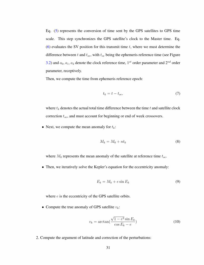
• Time system: In the GPS system, an important parameter is the GPS time, that

contains the calculations and measurements made by the control segment. The

SV clock and the user (GPS receiver) clock are running at slightly different rates

compared to the GPS time. The goal of synchronization using GPS system is to

make the corrected user clocks and the SV clocks reach this time as close as possible

[39].

28

Figure 3.2: Description of SV position from orbital parameters [39]

• Satellites movement: The satellites move around the earth because of a balance of

different forces. Under the assumption that the earth is a homogeneous sphere, the

centripetal force by the earth keeps the satellites in orbit. Perturbation force makes

the satellites slightly deviate from the orbit.

• Parameters: The non-disturbed motion of the satellite is based on Newton’s laws of

motion and gravitation and Kepler’s laws for orbits. The following six parameters

which are called orbital elements are required to uniquely identify a specific orbit:

A: Semi-major axis of the satellite orbit.

e: Eccentricity of the satellite orbit.

A and e: determine the shape and size of the Kepler ellipse.

Ω0: Longitude of ascending node of orbit plane at weekly epoch.

i0: Inclination angle at reference time.

29

Ω0 and i0: identify the satellite orbit plane and the relative orientation to the earth.

ω: Argument of perigee which represents the angle within the satellite orbit plane.

vk: True anomaly, which is the angle between the direction of periapsis and the

current position of the body, as seen from the main focus of the ellipse (the point

around which the object orbits).

The following parameters, which will be explained later, are also contained in the

navigation data for the correction of disturbed motion and clock: ∆n, a0, a1, a2, toc,

M0, cus, cuc, crs, crc, cis, cic, IDOT , Ω ,Ωe.

To calculate the satellite position, we proceed as follows [38]: 1. Evaluate the true

anomaly of the satellite, vk:

• Compute the mean angle velocity of the satellite:

n = n0 + ∆n (3)

where no is given by:

n0 =

√µ(√A)3 , (4)

µ represents the value of the earth universal gravitational parameter in WGS-84 for

the GPS user (µ = 3.986005×1014meters3/sec2), and ∆n is the mean angle velocity

difference between the value calculated from the navigation data and that calculated

from the Newton’s law and Kepler’s law.

• Correct the satellite clock at the observation time t′:

t = t′ −∆t (5)

∆t = a0 + a1(t− toe) + a2(t− toe)2 (6)

30

Eq. (5) represents the conversion of time sent by the GPS satellites to GPS time

scale. This step synchronizes the GPS satellite’s clock to the Master time. Eq.

(6) evaluates the SV position for this transmit time t, where we must determine the

difference between t and toe, with toe being the ephemeris reference time (see Figure

3.2) and a0, a1, a2 denote the clock reference time, 1st order parameter and 2nd order

parameter, receptively.

Then, we compute the time from ephemeris reference epoch:

tk = t− toe, (7)

where tk denotes the actual total time difference between the time t and satellite clock

correction toe, and must account for beginning or end of week crossovers.

• Next, we compute the mean anomaly for tk:

Mk = M0 + ntk (8)

where M0 represents the mean anomaly of the satellite at reference time toe.

• Then, we iteratively solve the Kepler’s equation for the eccentricity anomaly:

Ek = Mk + e sinEk (9)

where e is the eccentricity of the GPS satellite orbits.

• Compute the true anomaly of GPS satellite vk:

vk = arctan(

√1− e2 sinEkcosEk − e

) (10)

2. Compute the argument of latitude and correction of the perturbations:

31

• The argument of latitude, which is an angular parameter that defines the position of

a satellite moving along the orbit is given by:

Φk = vk + ω (11)

where ω denotes the argument of perigee given by the navigation data.

• Calculate the second harmonic perturbations, namely the argument of latitude

correction δuk, radius correction δdk and inclination correction δik.

δuk = cus sin 2Φk + cuc cos 2Φk

δrk = crs sin 2Φk + crc cos 2Φk

δik = cis sin 2Φk + cic cos 2Φk

(12)

where cus, cuc denote the amplitude of the sine/cosine harmonic correction term to

the argument of latitude.

crs, crc denote amplitude of the sine/cosine harmonic correction term to the orbit

radius.

cis, cic denote amplitude of the sine/cosine harmonic correction term to the angle of

inclination.

3. Compute the argument of latitude uk, radial distance rk, and the inclination ik:

uk = Φk + δuk

rk = A(1− e cosEk) + δrk

ik = i0 + δik + (IDOT )tk

(13)

where IDOT denotes the rate of inclination angle.

4. Calculate the position of satellite in ECEF:

32

• The satellite positions in orbital plane is given by:

xk′ = rk cosuk

yk′ = rk sinuk

(14)

• Compute the longitude of the ascending node Ωk with respect to Greenwich, which

is the angle from a reference direction, called the origin of longitude, to the direction

of the ascending node, measured in a reference plane. This calculation uses the right

ascension at the beginning of the current week Ω0, the correction from the apparent

sidereal time (a time scale that is based on the earth’s rate of rotation measured

relative to the fixed stars rather than the Sun), variation in Greenwich between the

beginning of the week and reference time tk = t − toe, and the change in longitude

of the ascending node from the reference time toe:

Ωk = Ω0 + (Ω− Ωe)tk − Ωetoe (15)

where Ω denotes the rate of right ascension and Ωe is WGS-84 value of the earth’s

rotation rate (Ωe = 7.2921151467× 10−5rad/s).

• Compute the earth-fixed coordinates:

xk = xk′ cos Ωk − yk ′ cos ik sin Ωk

yk = xk′ sin Ωk − yk ′ cos ik cos Ωk

zk = yk′ sin ik

(16)

5. Identify the visible satellites:

• Check which satellites are visible to the test point: As shown in Figure 3.3, r is the

radius of earth and R is the radius of satellites orbit. Given the position of the fixed

33

Figure 3.3: Visible satellites from a fixed elevation angle

GPS-receiver location xrec, yrec and the cut-off angle α, the elevation angle of the

satellites β can be calculated as:

β = arctgcos(xk − xrec) cos yrec − 0.15127√

1− [cos(xk − xrec) cos yrec]2

(17)

If the elevation angle of the GPS satellite β is not larger than the elevation angle of

the reference point βrec, the considered satellite is visible.

3.3 Simulation Results

In order to verifiy the feasibility of our approuch, we use the matlab tool – GPS satellite

visibility to predict the visible satellites from the EV building at the Concordia University.

To run the navigation tool, we need to provide the observed GPS receiver’s position

and time period, which include latitude, longitude, height and cut-off angle and date.

Then, an almanac file describing the orbits of the GPS satellites is also needed, where [40]

provides the almanac files updated daily for users to download. The program produces

comprehensive charts and reports of GPS satellite visibility for a 24-hour period (e.g.,

see Figure 3.4). Figure 3.5 shows the visible satellites that are visible from EV building,

Concordia University, Montreal, Quebec, Canada, GSW campus, with a cut-off angle of 15

34

degrees on July 12th, 2016.

We input the following information to the GPS satellite visibility:

Station: Montreal Latitude: 45.8294 Longitude: -73.9622 Height: 124 Cut-off

angle: 15 Timezone: -5 Date: 2016/07/12 Duration: 0:00 — 24:00

Figure 3.4: Prediction of the appearance of visible satellites

Station: Montreal Latitude: 45.8294 Longitude: -73.9622 Height: 124

Cut-off angle: 15 Timezone: -5 Date: 2016/07/12 Duration: 0:00 — 24:00

Figure 3.5: Prediction of the number of visible satellites

Figure 3.4 provides us the details of the visibility of each satellite in 24 hours at

35

Concordia University. X axis represents time (hour), Y axis is the serial number of the

satellites (from 1 to 32), red area denotes the appearance of the corresponding satellites.

As depicted in Figure 3.5, during the entire time period of the position we choose, at least

five satellites could be seen at the same time. In fact, 4 satellites are enough for a GPS

receiver to compute the position and time information, and more satellites are visible at the

same time, the more accurate the solutions.

Moreover, if higher accuracy is desirable, another type of errors should also take

into account. Errors affect the satellites’s orbit or ephemeris are called ephemeris errors,

which are caused by gravitational pulls from the moon and sun and by the pressure of

solar radiation on the satellites. These types of errors are usually very slight. One can

use the data available from the International GNSS (Global navigation satellite system)

Service (IGS) which collects, archives, and distributes GPS and GLONASS (Russian

Global Navigation Satellite System) observation data sets from varieties of analysis centers

for better prediction accuracy.

3.4 Counclusion

The GPS spoofer sends simulated GPS signals to attack a GPS receiver which will

lead a false time solution for PMUs. Throughout this chapter, we have explained an

algorithm which utilizes the navigation data from the GPS signals and basic rules of

satellites movement in the space to predict the visible satellites of a fixed location and a

given time period. Within this context, we proposed a methodology for the GPS receiver to

detect the received simulated signal which has different C/A code and a different one of the

visible satellites. Our simulation results confirm the feasibility of the proposed approach.

However, it should be noted that, the visible satellites prediction countermeasure is

ineffective for the type of spoofing attacks that only modify the parameters in the navigation

data, but contain the same C/A code with the visible satellites. In order to further enhance

36

the robustness of GPS-based PMUs, in the next chapter we propose another detection

algorithm that resists this type of attacks.

37

Chapter 4

Anomaly Detection of Data-Level GPS

Spoofing

Because of the system noise, the differences between two consecutive time solutions

are unlikely constant. In this chapter, we assume that the random error between the time

solutions of GPS receiver follows a Gaussian distribution. According to Total Vector Error

(TVE) given by the IEEE C37.118 standard, we set up a model of the difference values

between two consecutive time solutions. Also, we model the GPS data-level spoofing and

analyze the changes in the time differences after the appearance of the attacks. Finally, the

effectiveness of the proposed technique is confirmed by simulations.

4.1 GPS-PPS Stochastic Error Analysis

In phasor measurement unit, we require one Pulse-Per-Second(PPS) synchronization

signal provided by GPS receivers. However, the clock in each GPS receiver may drift apart

or gradually desynchronize from the master time with different drift rates. Therefore, one

needs to use the GPS system with highly accurate atomic clocks (inside the GPS satellites)

to synchronize the GPS receiver’s clock. We divide the deviations of a GPS receiver clock

38

into two categories: the systematic effects such as the time drift, as well as the random

errors such as white noise. Based on the fact that we have already known the position of

the GPS receiver, in our approach, we describe the time solution by a simple model:

c × ∆ttrans,k = dtrue,k + c × tb,k (18)

tmeas,k = trcv,k − tb,k (19)

where trcv,k denotes the time provided by the internal clock of the GPS receiver at time k,

∆ttrans,k denotes the signal propagation time from the GPS satellites to the GPS receiver at

time k (calculated during the code tracking part), dtrue,k represents the true range between

visible GPS satellite and GPS receiver, tb,k is the time bias between GPS satellites clock

system and the GPS receiver internal clock, and tmeas,k is the synchronized time solution

of the GPS receiver. Hence, the error in time is given by:

ek = tmeas,k − t true,k (20)

The IEEE C37.118 standard [41] requires the accuracy of the time solution should be within

the range of ek ≤ 40 ns for 95% of the values. And according to this standard, a time error

of 1 µs corresponds to a phase error of 0.022 degrees for a 60 Hz system and 0.018 degrees

for a 50 Hz system. Also, phase error of 0.57 degrees (0.01 radian) will by itself cause 1%

TVE. In what follows, we assumes that the random error ε between the time solutions of

GPS receiver and the UTC follows a Gaussian distribution ek ∼ N(0, σ2).

In order to check whether the error of time solutions are within a reasonable range,

given the real UTC time and the system noise are unknown, we will induce the pseudo-error

ek. Different from the real error between the time solutions and UTC time, we randomly

choose a start point of the time solutions from GPS receiver, then calculate the pseudo-error

39

as follows:

ek = tmeas,k − tmeas,1 − (k − 1) k = 1, 2, 3... (21)

According to our simulation results, the distribution of ek also follows a normal distribution.

Then, the sample mean of the pseudo-error is given by

µ = tek =

n∑k=1

(ek)

n(22)

4.2 Models of Attacks

GPS spoofers can manipulate the results of the receiver position, ephemerides, satellite

positions, and pseudo-ranges by broadcasting falsified GPS signals and forcing the GPS-

based PMU receiver to track the falsified signals. This spoofer-induced timing offset

creates a corresponding change in the phase measured by the PMUs.

As mentioned in chapter 2, there are several types of spoofing attacks which include signal-

level spoofing, data-level spoofing, and bent-pipe spoofing.

In this chapter, our proposed countermeasure is mainly against those attacks which

change the navigation data. According to Equation (18), the data-level spoofing changes

the information about satellite’s position and further leads to incorrect clock bias tb,k. It can

also spoof arbitrary number of satellite signals and introduce a receiver clock offset error

without significantly changing the computed receiver position from its pre-attack value.

According to the structure of the navigation data sent by the GPS satellites [42], the

GPS receivers will continuously receive the signals and refresh one sub-frame of navigation

information for 30 seconds. As a result, different types of errors may occur. Following are

three possible types of spoofing attacks that we consider:

a) Scaling Attack:

For this type of attack, the error caused by the spoofer will sharply increase (or decrease)

40

Figure 4.1: Example of Scaling attack, ramp attack, and random attack

and will continue with the same error value,

wk = p, k ≥ n (23)

where wk denotes the error value at the ith epoch and p is the spoofing error value.

b) Ramp Attack:

Here, the attacker will gradually increase (or decrease) the error value, rendering the time

solution to exceed the threshold. This type of attack is described as follows,

wk = pk +m×∆p, k ≥ n, m = 1, 2, 3... (24)

where ∆p is the error changing rate. Here the error value is continuous for a time length of

integer multiple of 30 seconds.

c) Random Attack:

The error will change discontinuously and gradually until it passes the threshold.

41

4.3 Proposed Anomaly Detection Scheme

As mentioned in Section 4.1, we assume that the GPS receiver’s time solution follows a

normal distribution for a random sample from the entire population. Also, there is enough

evidence that the pre-attack values of the pseudo-error follow a normal distribution. In

this work, the abnormal value of the time solution caused by a spoofing attack would be

determined by a binary hypothesis testing.

The process is that, when we observe a sample of time solutions, we use hypothesis

testing to determine whether there is enough evidence to infer that a certain condition is true

for the entire population. However, to examine the whole population is often impractical.

Therefore, we examine a random sample from the population. If the results calculated

from the sample data are not consistent with the statistical hypothesis, the hypothesis is

rejected. There are two types of statistical hypotheses: The null hypothesis, denoted by

H0, represents the hypothesis that the time solution at the moment is consistent with the

learnt statistics of the receiver’s clock. The alternative hypothesis, denoted by H1 or Ha, is

the hypothesis that the pseudo-error has exceeded the threshold which means the system is

influenced by the attacker [43].

For the first part of our proposed anomaly detection, we will use the sample mean to

estimate the population mean of the pseudo-error, and then compare it to the upcoming

values of the pseudo-error. Let n denote the number of samples. According to (22), after n

samples, we use upcoming values ek (k > n) to compare with the sample mean µ.

H0: ek = µ

H1: ek 6= µ

Let α1 denotes the false alarm rate according to the system design requirements, and λ1

denotes the corresponding threshold calculated from the distribution of pseudo-error. As

shown in Figure 4.2, if ek is out of the acceptance region, we conclude that the time solution

at time k is calculated from the spoofed signal.

42

Figure 4.2: Hypothesis testing of anomaly detection 1

The second part of the detection allows us to test if the GPS receiver is under the ramp

attack following the procedure below.

• As mentioned in the first part, we calculate the sample mean of the pseudo-error.

• Count the number of upcoming pseudo errors that are larger than the sample mean in

the considered sliding window analysis:

NL j = # j −NT < k ≤ j|ek > µ (25)

where NL j represents the number of samples larger than the threshold in the shifting

window.

• Calculate the ratio of larger samples:

rj = NL j/NT (26)

where NT is the number of samples in the sliding window.

43

• Let α2 denote the false alarm rate for the slope detection system and let λ2 denote

the corresponding threshold. The value of the ratio at time j equal rj .

H0:rj = 0.5

H1:rj 6= 0.5

For the unspoofed receiver, Figure 4.3 shows the ratio from which we can conclude

that if there is no spoofer attacks, the ratio result of the second part should be around

the 0.5.

Figure 4.3: Pre-attacked Ratio value

As shown in Figure 4.4, when an attack occurs, the ratio of the samples larger/less

than the sample mean within a shifting window will no longer keep a balance.

If the ratio we tested falls in the acceptance region (H0), then the system has not been

spoofed or the influence of the spoofing attack is not large enough to cause an unacceptable

44

Figure 4.4: Spoofed Ratio value

Figure 4.5: Hypothesis testing of the anomaly detection part2

error to the PMU. Note that H1 represents a warning area in this scenario, if rj is in the

rejection region, the time solution at time j is labelled as being spoofed (Figure 4.5).

45

Figure 4.6: Flow chart of anomaly detection algorithm

46

The flow chart of the detection algorithm is shown in Figure 4.6. When the algorithm

declares that the GPS receiver has been spoofed, there are different methods to locate

the spoofer [44]. Also, there are methods to improve the stability of the PMU clock, for

example, according to [45], after disconnecting the link, the PMU can operate stably for a

period of several hours. In this case, we can restart the GPS receiver, refresh the navigation

data and check for spoofing again.

4.4 Simulation Results

The simulation environment used for performance investigation is as follow:

• Accuracy of the time solution: ek ≤ 40 ns for 95% of the values.

• Number of samples for the sample mean: 300 samples.

• Shifting window for the slope detection: 150 samples.

Figure 4.7 depicts the Receiver-Operating Characteristics (ROC) curves of our anomaly

detection for the scaling attack. From our simulation results, it can be seen that the error

caused by the scaling attack can be effectively detected when it is larger than about 120ns,

which is smaller than the threshold defined by the IEEE C37.118 standard. For the ramp

attack, the system can detect the attack with a zero miss-detection rate. The simulation

results show that our anomaly detection is an effective countermeasure against the data-

level spoofing.

The advantage of the anomaly detection is due the fast detection time against the

different types of data-level spoofing. Figure 4.8 shows that the detection time of different

errors increasing/decreasing rate caused by the attacker. According to our proposed

algorithm, the system will give us a warning of spoofing attack when one of the results

of two parts falls in the rejection region. Thus, the detection time of the algorithm is equal

to the minimum of the two sub-detection systems.

47

Figure 4.7: ROC curve of detect the scaling attack

Figure 4.8: Detection time of anomaly detection

48

4.5 Conclusions

The stability of time solutions provided by GPS receiver is essential to PMU sampling

precision and time-stamps of the measurements. In this chapter, we assume that the time

solutions will follow a Gaussian distribution, so that we can detect the abnormal trend of

the pseudoerror and provide a warning of spoofing attack. Based on our simulation results,

we can draw a conclusion that the proposed anomaly detection can detect a scaling attack

when the errors caused by the attacker exceeds the threshold based on the real needs of

the system. Also, we can detect a spoofing attack when there is a continuous trend of

increase/decrease of the error.

49

Chapter 5

FFT-Dased Detection

In the previous two chapters, we have proposed two approaches for the detection of

spoofing attacks at the GPS receiver side. These two solutions, however do not utilize the

information that can be obtained by correlating the information from multiple PMUs at

the PDC side. In this chapter, we analyze the impact of the GPS spoofing attacks on the

relative phase angle differences between two PMU stations. Then, we propose a spoofing

detection technique which compares the synchrophasor data from multiple PMUs. We use

real PMU data from the Texas synchrophasor network to verify the effectiveness of our

proposal approach.

5.1 Background of Synchrophasor Networks

5.1.1 Phasor measurement unit

As we mentioned earlier, the development of the Phasor Measurement Units started

in the 1990s in order to improve the accuracy and performance of power system state

estimation. PMUs measure the system voltage magnitude and phase angle at a given station

and upload the phasor information to PDC at a rate of 30 or 60 samples per second.

50

Figure 5.1: Block diagram of a PMU [13]

Figure 5.1 shows a basic hardware block diagram of a PMU. The analog AC waveforms

are digitized by an Analog to Digital Converter for each phase. A phase-locked oscillator,

along with a Global Positioning System reference source, provides the needed high-speed

synchronized sampling with 1-microsecond accuracy. The GPS receiver provides one pulse

per second (1-PPS) to the oscillator which divides the signal into the required sampling

rate. This GPS system is designed primarily for navigational purposes, but it furnishes a

common-access timing pulse, which is accurate to within 1 microsecond at any location

on earth [46]. Besides, the voltage magnitude and current phasors are calculated by digital

signal processing techniques.

5.1.2 Synchrophasor and PMU data

The synchrophasor representation of the signal x(t) in Equation (1) is the value X in

Equation (2), where φ is the instantaneous phase angle relative to a cosine function at the

nominal system frequency synchronized to UTC [41]. All measurements from different

PMUs are synchronized to a common time base with a common frequency, which makes

the phase angle measurements directly comparable. Synchrophasors change over time

unless the signal is a pure sinusoid with a frequency equal to the nominal system. A precise

51

time reference (clock) is required to provide the UTC time to determine the phase angle φ

[41].

The University of Texas at Austin (UT-Austin) introduced an independent syn-

chrophasor network (Figure 5.2) to monitor abnormal events and analyze low-frequency

oscillations from the electric power grid through PMU measurements taken at the customer-

level voltage (120 V)[12].

Figure 5.2: Map of texas PMU stations within the UT-Austin independent texassynchrophasor network [12]

The time-stamped phasors from each PMU station are sent either through the public

Internet or serial cables to the phasor data concentrators. The phasor data concentrator

waits for data from all PMUs and stores the PMU data once it is received. These data

points are stored hourly in a comma-separated value (CSV) format. The synchrophasor

network is in operation at all times.

Figure 5.3 shows an example of a PMU data file associated with PMU measurements.

All measurements are taken at the customer-level voltage of 120 V [12]. The first

52

column represents the time-tag provided by the GPS receiver, the other columns denote

the magnitude, phase angle and frequency, respectively.

Figure 5.3: Example of PMU data format [12]

The IEEE 37.118.1-2011 standard covers the measurement provisions and is intented to

describe and quantify the performance of PMUs instrument deployed to monitor the power

grid [41].

5.2 Proposed FFT-based Detection Algorithm

Our proposed detection algorithm is based on analyzing the relative phase angle

difference between two PMU stations. The procedure is described as follows:

5.2.1 Relative phase angle difference

Because the rotation of the voltage phasors is not constant, that is to say it is not fixed at

a nominal frequency, the voltage phase angle varies depending on the the speed of rotation

the associated generators.

In Figure 5.4, the x-axis represents the time, and y-axis represents the value of voltage

phase angle. When the voltage phasor is rotating at greater-than-nominal speed and crosses

from 180 to -180 degrees, the voltage phase angle jumps. For our simulation, we need first

to unwrap the voltage phase angle at each PMU station before the difference in the voltage

phase angle between the two stations can be calculated.

In Figure 5.5, the blue curve represents the unwrapped phase angle, which is clearly

a smoother phase plot than the red one. The unwrapping function is implemented by the

53

Figure 5.4: Raw PMU phase data

Figure 5.5: Raw PMU phase angle and unwrapped curve

Matlab function Q = unwrap(P). This function corrects the phase angles in a vector P by

adding multiples of ±2π when the difference between consecutive P are greater than or

54

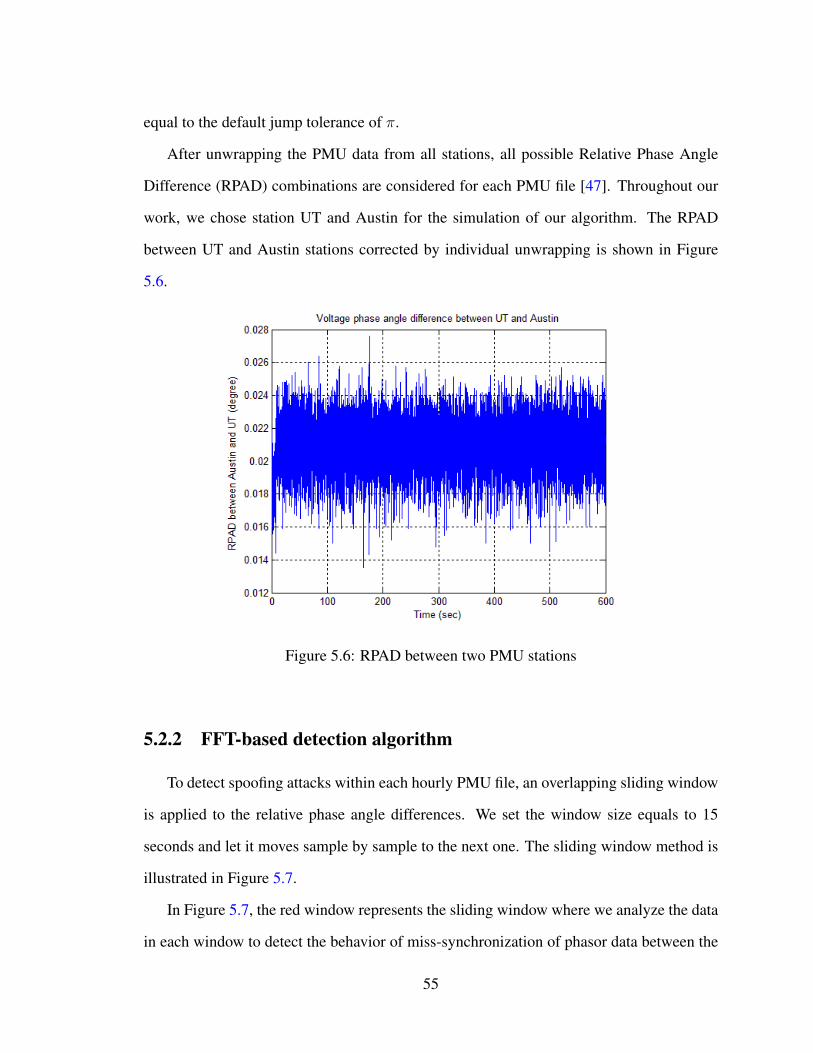
equal to the default jump tolerance of π.

After unwrapping the PMU data from all stations, all possible Relative Phase Angle

Difference (RPAD) combinations are considered for each PMU file [47]. Throughout our

work, we chose station UT and Austin for the simulation of our algorithm. The RPAD

between UT and Austin stations corrected by individual unwrapping is shown in Figure

5.6.

Figure 5.6: RPAD between two PMU stations

5.2.2 FFT-based detection algorithm

To detect spoofing attacks within each hourly PMU file, an overlapping sliding window

is applied to the relative phase angle differences. We set the window size equals to 15

seconds and let it moves sample by sample to the next one. The sliding window method is

illustrated in Figure 5.7.

In Figure 5.7, the red window represents the sliding window where we analyze the data

in each window to detect the behavior of miss-synchronization of phasor data between the

55

Figure 5.7: Sliding window

Figure 5.8: FFT of RPAD between two stations

two stations. There are 450 samples in one sliding window at time t, and we apply the

FFT function to those RPAD values in this window. Then, we move the window forward to

the next sample. This Discrete Fourier Transform shows us all the frequency components

within one sliding window. Figure 5.8 shows the FFT result for the case of no attack. Figure

56

5.9 shows the corresponding FFT results in the case of a spoofing attack. It is clear that

when the sliding window moves on, the low frequency components of the FFT increase. In

our algorithm, we consider that the changes of RPAD caused by spoofing attacks on GPS

receiver are reflected in the changes of the low frequency value of the FFT.

Figure 5.9: FFT results after spoofing attack

To begin with, we analyze the distribution of low frequency value of pre-attack RPAD.

We choose the low frequency components for our simulation. Based on an entire hourly

data of the real phasor data from the Texas Synchronphasor Network, we applied the

FFT to the RPAD between UT and Austin stations. Figure 5.10 shows the probability

density function of the low frequency components of the RPAD signal. From the figure,

we conclude that the pre-attacked low frequency value follows a Gaussian distribution.

Figure 5.11 represents the flow chart of the detection procedure.

5.2.3 Simulation results

The simulation environment used in our performance investigation is as follow:

57

Figure 5.10: PDF of the low frequency components of the RPAD signal

• PMU data from Texas Synchrophasor Network PMUs

• Sliding window length: 15 seconds

• Reporting rate of the PMU data: 30 samples per second

For the next step, we add the spoofing attacks to the system. We applied three types

of the spoofing attack, including the scaling attack, ramp attack and random attack. The

errors in the time-stamps provided by the GPS receivers are added to the time column of

raw phasor files of the UT station. Then, we apply the FFT to the RPAD data within each

sliding window and record the values of the low frequency components. After that, we use

binary hypothesis testing to determine if there is an abnormal value caused by a spoofer.

Figure 5.12 shows an example for how the curve of low frequency component changes

during a spoofing attack. Also, the simulation result shows that, for all the time errors

caused by different types of spoofing attacks, there is always a clear increase in the low

frequency components after the attack happened.

58

Figure 5.11: Flow chart of the detection procedure

59

Figure 5.12: Trend of low frequency changes during attack

The threshold used to determine whether there is a spoofing attack is based on the need

of different systems. The false alarm rate of the FFT detection algorithm is shown in Figure

60

Figure 5.13: False alarm rate of detection algorithm

61

the proposed FFT detection algorithm can effectively detect spoofing attacks.

results from the detection method are based on a time period of one hour, and it shows that

the unwrapped RPAD, we can detect the changes caused by the GPS spoofing attacks. The

synchrophasor network stations for the power system. By applying a sliding window of

detect the RPAD abnormal changes. We used the real PMU data from UT and Austin

angle differences between two PMU stations. We proposed an algorithm which aims to

In this chapter, we explained the influence of the spoofing attacks to the relative phase

5.3 Conclusion

threshold.

, where the x axis represents the false alarm rate while the y axis denotes the detection5.13

Chapter 6

Conclusions and Future Work

Time stamps provided by the GPS receivers to the PMUs are vital to the proper

operation of Wide Area Mornitoring Systems. A GPS spoofer transfers incorrect GPS

signals, which resembles the normal GPS signals, but with different receiver position,

ephemerides, satellite position or the pseudo-range. Afterwards, miss-synchronized phasor

data will influence the result of the state estimation of the power system, which will

further cause errors in the distribution automation. In this thesis, we mainly focus on

the countermeasures against GPS spoofing attacks at the GPS receiver-side and the data

concentration center side. In order to enhance the robustness of the GPS-based PMUs, we

propose three methods to detect spoofing attempts.

The GPS receiver will recognize the visible satellites by correlating the local generated

C/A codes and the received signals. In this context, we proposed a method for predicting

the visible satellites at a given location and time period. Using the navigation messages, the

time of the observation, and the basic physics of satellite motion in the space, we predict

the number of visible satellites to prevent the GPS receiver from tracking manipulated

signals. The approach enhances the security against attacks, as it reduces the chance for

the manipulated signals to pass to the data processing part.

Furthermore, based on the fact that the time period between two PPS signals should be

62

one second, we utilize the changes in the observed signal statistics when the system is under

attack to detect the presence of spoofing attempts. The second detection technique is mainly

against the data-level spoofing, which modifies the time information in the navigation

data. The simulation results confirm that our proposed anomaly detection algorithm can

effectively detect the data-level spoofing attacks.

Finally, after the PMUs upload the measurements to the phasor data concentrators,

we can detect the spoofing attacks based on the stability of RPAD between two PMU

stations. The low frequency components of the relative phase angle differences between

the two PMUs should be within a certain range, and that will increase in the case of miss-

synchronization. Our simulation results shows that when the spoofing happens, the low

frequency components of RPAD increase, which makes the detection of attacks feasible.

It should be noted that, although we have considered the sensitivity and the timeliness

of our proposed countermeasures, in reality, the cost and computational complexity should

also be taken into account. One possible area of research would be the utilization of

prediction techniques such as Kalman filter to predict the timing information provided

by the GPS receiver. Kalman filter can predict the time information of the next time

epoch based on a series of measurements observed over time. Theoretically, the difference

between time information and the prediction value would be no larger than the tolerance

given by IEEE standard.

Another possible area of improvement would be the investigation of cross-detection

among multiple GPS receivers. It is difficult for one GPS spoofer to spoof multiple GPS

receivers. Consequently, linking several GPS receivers through a communication network

and cross-checking the time information calculated by each receiver can provide a good

countermeasue against spoofing attacks. In order to apply this improvement, we need

to ensure the security and minimize the time delay during the information transmission

between the GPS receivers.

63

Bibliography

[1] “Electric Power System.” https://en.wikipedia.org/wiki/Electric_

power_system#cite_note-1, 2016.

[2] Xi Fang, Satyajavant Misra, Guoliang Xue, Dejun Yang, “Smart Grid - The New

and Improved Power Grid: A survey,” IEEE Communications Surveys and Tutorials,

vol. 14, pp. 944 – 980, Dec. 2012.

[3] Cai, Jim Y., Zhenyu Huang, John Hauer, Ken Martin, “Current Status and Experience

of WAMS Implementation in North America,” (Dalian), pp. 1 – 7, Transmission and

Distribution Conference and Exhibition: Asia and Pacific, 2005 IEEE/PES, IEEE,

Aug. 2005.

[4] Narayanan, K Shankar, Ravipudi Sudhir, Yogesh Kanna, “WAMS - Mitigating

Angular Instability in Large Interconnected Power Systems,” in 2015 Saudi Arabia

Smart Grid (SASG), pp. 1 – 5, IEEE, Dec. 2015.

[5] Xichen Jiang, Jiangmeng Zhang, Brian J. Harding, Jonathan J. Makela, Alejandro D.

Dom ınguez-Garcıa, “Spoofing GPS Receiver Clock Offset of Phasor Measurement

Units,” IEEE Transactions on Power Systems, vol. 28, pp. 3253 – 3262, Aug. 2013.

[6] Zhenghao Zhang, Shuping Gong, Aleksandar D. Dimitrovski, Husheng Li, “Time

Synchronization Attack in Smart Grid: Impact and Analysis,” IEEE Transactions on

Smart Grid, vol. 4, pp. 87 – 98, Mar. 2013.

64

[7] Jon S. Warner, Roger G. Johnston, “GPS Spoofing Countermeasures,” Homeland

Security Journal, vol. 25, no. 2, pp. 19 – 27, 2003.

[8] Nathan Alan White, Peter S. Maybeck, Stewart L. DeVilbiss, “Detection of

Interference/Jamming and Spoofing in A DGPS-aided Inertial System,” IEEE

Transactions on Aerospace and Electronic Systems, vol. 34, pp. 1208 – 1217, Oct.

1998.

[9] Paul. Y. Montgomergy, Todd. E. Humphreys, Brent. M. Ledvina, “Receiver-

Autonomous Spoofing Detection: Experimental Results of a Multi-antenna Receiver

Defense Against a Portable Civil GPS Spoofer,” (Anaheim), pp. 26 – 28, ION 2009

International Technical Meeting, Jan. 2009.

[10] Mark L. Psiaki, Steven P. Powell, Brady W. O’hanlon, “GNSS Spoofing Detection

Using High-frequency Antenna Motion and Carrier-phase Data,” in 26th International

Technical Meeting of The Satellite Division of the Institute of Navigation (ION GNSS+

2013), (Nashville), pp. 2949 – 2991, Sep. 2013.

[11] Kyle Wesson, Mark Rothlisberger, Todd Humphreys, “Practical Cryptographic Civil

GPS Signal Authentication,” Navigation, vol. 59, pp. 177 – 193, Fal. 2012.

[12] A. Allen, S. Santoso, Eduard. Muljadi, “Algorithm for Screening Phasor

Measurement Unit Data for Power System Events and Categories and Common

Characteristics for Events Seen in Phasor Measurement Unit Relative Phase-Angle

Differences and Frequency Signals,” technical report, National Renewable Energy

Laboratory, Aug. 2013.

[13] Liang Heng, Jonathan J. Makela, Alejandro D. Domınguez-Garcıa, Rakesh B.

Bobba, William H. Sanders, Grace Xingxin Gao, “Reliable GPS-based Timing for

65

Power Systems: A Multi-layered Multi-receiver Architecture,” in Power and Energy

Conference at Illinois (PECI), 2014, (Urbana), pp. 1 – 7, IEEE, Mar. 2014.

[14] T. L. Bitner, “Detection and Removal of Erroneous GPS Signals Using Angle of

Arriva,” Master’s thesis, Auburn University, Auburn, Dec. 2013.

[15] Nils Ole Tippenhauer, Christina Ppper, Kasper Bonne Rasmussen, Srdjan Capkun,

“On the Requirements for Successful GPS Spoofing Attacks,” in CCS’11 18th ACM

conference on Computer and communications security, (Chicago, Illinois, USA),

pp. 17–21, Oct. 2011.

[16] “Texas Synchrophasor Network.” http://web.ecs.baylor.edu/faculty/

grady/Texas_Synchrophasor_Network.html, 2016.

[17] “Flashnet.” http://www.flashnet.ro/project/inteligrid.

[18] Trevor M. Letcher, ed., Future Energy: Improved, Sustainable and Clean Options for

our Planet. Elsevier Science, 2 ed., Dec. 2013.

[19] Tariq Samad, Sila Kiliccote, “Smart Grid Technologies and Applications for the

Industrial Sector,” Computers and Chemical Engineering, vol. 47, pp. 76 – 84, Dec.

2012.

[20] Murtaza Hashmi, Seppo Hanninen, Kari Maid, “Survey of Smart Grid Concepts,

Architectures, and Technological Demonstrations Worldwide,” in Innovative Smart

Grid Technologies (ISGT Latin America), 2011 IEEE PES Conference on, (Medellin),

pp. 1 – 7, IEEE, Oct. 2011.

[21] Denzil Walton, “Smart Grid: A Grid Suitable for Renewable

Energy.” http://www.leonardo-energy.org/blog/

smart-grid-grid-suitable-renewable-energy, Feb. 2015.

66

[22] Normazlina Binti Mat Isa, Tan Chee Wei, Abd Halim Mohd Yatim, “Smart

Grid Technology: Communications, Power Electronics and Control System,” in

2015 International Conference on Sustainable Energy Engineering and Application

(ICSEEA), (Bandung), pp. 10 – 14, Oct. 2015.

[23] “Understanding the Benefits of the Smart Grid,” technical report, National Energy

Technology Laboratory, 2010.

[24] International Energy Agency, “Technology Roadmap: Smart Grids,” technical report,

Nov. 2011.

[25] Aaron St. Leger, Jeremy Spruce, Thomas Banwell, Michael Collins, “Smart Grid

Testbed for Wide-Area Monitoring and Control systems,” in 2016 IEEE/PES

Transmission and Distribution Conference and Exposition (T&D), (Dallas, TX,

USA), pp. 1 – 5, May 2016.

[26] Kun Zhu, Moustafa Chenine, Johan Konig, Lars Nordstrom, “Analysis of Data

Quality Issues in Wide Area Monitoring and Control Systems,” in Bulk Power System

Dynamics and Control (iREP) - VIII (iREP), 2010 iREP Symposium, (Rio de Janeiro),

pp. 1 – 8, Aug. 2010.

[27] Ye Yan, Yi Qian, Hamid Sharif, David Tipper, “A Survey on Smart Grid

Communication Infrastructures: Motivations, Requirements and Challenges,” IEEE

Communications Surveys & Tutorials, vol. 15, pp. 5 – 20, Feb. 2013.

[28] Yiwei Ma, Ping Yang, Hongxia Guo, “Distributed Generation System Development

Based on Various Renewable Energy Resources,” in Control Conference (CCC), 2011

30th Chinese, (Yantai), pp. 6203 – 6207, Jul. 2011.

67

[29] Janaka Ekanayake, Nick Jenkins, Kithsiri Liyanage, Jianzhong Wu, Akihiko

Yokoyama, Smart Grid: Technology and Applications. John Wiley and Sons, Apr.

2012.

[30] Liu Wenxia, Fan Yongfeng, Zhang Lixin, Zhang Xin, Que Huakun, “WAMS

Information Security Assessment Based on Evidence Theory,” in 2009 International

Conference on Sustainable Power Generation and Supply, (Nanjing), pp. 1 – 5, Apr.

2009.

[31] Phasor Real Time Dynamics Mornitoring System. http://www.

phasor-rtdms.com/phaserconcepts/phasor_adv_faq.html.

[32] Kal Kaur, “Understanding the Global Positioning System,” technical report,

AZoSensors, Jul. 2012.

[33] Dillon Gere, Francis Juelar, AAron Mcclanahan, “The Transmission

of GPS Signals.” http://ee3550-gps.weebly.com/

transmission-of-gps-signals.html.

[34] Alexander Ruegamer, Dirk Kowalewski, “Jamming and Spoofing of GNSS Signals–

An Underestimated Risk,” From the Wisdom of the Ages to the Challenges of the

Modern World Sofia, pp. 17 – 21, May 2015.

[35] Ali Jafarnia-Jahromi, Ali Broumandan, John Nielsen, Gerard Lachapelle, “GPS

Vulnerability to Spoofing Threats and A Review of Antispoofing Techniques,”

International Journal of Navigation and Observation, vol. 2012, pp. 1 – 16, May

2012.

[36] Fu Zhu, Amr Youssef, Walaa Hamouda, “Detection Techniques for Data-level

Spoofing in GPS-based Phasor Measurement Units,” in Selected Topics in Mobile

and Wireless Networking (MoWNeT), (Cairo), pp. 1 – 8, IEEE, Jun. 2016.

68

[37] Reynaldo Francisco Nuqui, State Estimation and Voltage Security Monitoring Using

Synchronized Phasor Measurements. PhD thesis, Virginia Polytechnic Institute and

State University, 2001.

[38] GPS.GOV, “Global Positioning Systems Directorate Systems Engineering and Inte-

gration, Interface Specification IS-GPS-200,” technical report, National Coordination

Office for Space-Based Positioning, Navigation, and Timing, Washington, D.C., Sep.

2013.

[39] Dan Doberstein, Fundamentals of GPS Receivers, A Hardware Approach. Springer-

Verlag New York, 1 ed., 2012.

[40] Thomas Sean Kelso, “GPS Yuma Almanacs 2016.” http://celestrak.com/

GPS/almanac/Yuma/2016/.

[41] IEEE Power and Energy Society, “C37.118.1-2011 - IEEE Standard for Synchropha-

sor Measurements for Power Systems,” pp. 1 – 61, Dec. 2011.

[42] Heidi Kuusniemi, User-level Reliability and Quality Monitoring in Satellite-based

Personal Navigation. PhD thesis, Department of Information Technology, Tampere

University of Technology, Finland, Jun. 2005.

[43] “What is Hypothesis Testing.” http://stattrek.com/hypothesis-test/

hypothesis-testing.aspx.

[44] Der-Yeuan Yu, Aanijhan Ranganathan, Thomas Locher, Srdjan Capkun, David Basin,

“Short Paper: Detection of GPS Spoofing Attacks in Power Grids,” in WiSec’14

Proceedings of the 2014 ACM Conference on Security and Privacy in Wireless and

Mobile Networks, (Oxford, UK), pp. 99 – 104, SIGSAC ACM Special Interest Group

on Security, Audit, and Control, Jul. 2014.

69

[45] Ning Wu, Xiaolong Pan, Jiexia Yu, “Research and Realization of the High Accuracy

GPS Synchronization Clock,” Automation of Electric Power Systems, vol. 10, pp. 1–

18, 2008.

[46] Arun G Phadke, “Synchronized Phasor Measurements - A Historical Overview,”

in Transmission and Distribution Conference and Exhibition 2002: Asia Pacific.

IEEE/PES, vol. 1, pp. 476 – 479, IEEE, Oct. 2002.

[47] A. Allen, M. Singh, S. Santoso, Eduard. Muljadi, “PMU Data Event Detection:

A User Guide for Power Engineers,” technical report, National Renewable Energy

Laboratory, Oct. 2014.

70