Detection of Variable Stars in the Open Cluster M11 …central.oak.go.kr/repository/journal/10773/OJOOBS_2010_v27n4_289.pdf · limitation as open codes, ... GEOTRAN. The first step

Copyright © The Korean Space Science Society 289 http://janss.kr pISSN: 2093-5587 eISSN: 2093-1409

Research Paper J. Astron. Space Sci. 27(4), 289-307 (2010)DOI: 10.5140/JASS.2010.27.4.289

Received Sep 24, 2010 Revised Oct 08, 2010 Accepted Oct 13, 2010†Corresponding Author

E-mail: [email protected] Tel: +82-42-865-3255 Fax: +82-42-865-3272

This is an Open Access article distributed under the terms of the Creative Commons Attribution Non-Commercial License (http://cre-ativecommons.org/licenses/by-nc/3.0/) which permits unrestricted non-commercial use, distribution, and reproduction in any medium, provided the original work is properly cited.

Detection of Variable Stars in the Open Cluster M11 Using Difference Image Analysis Pipeline

Chung-Uk Lee1†, Jae-Rim Koo1, Seung-Lee Kim1, Jae Woo Lee1, Byeong-Gon Park1, and Cheongho Han2

1Korea Astronomy and Space Science Institute, Daejeon 305-348, Korea2Department of Physics, Chungbuk National University, CheongJu 361-763, Korea

We developed a photometric pipeline to be used for a wide field survey. This pipeline employs the difference image

analysis (DIA) method appropriate for the photometry of star dense field such as the Galactic bulge. To verify the perfor-

mance of pipeline, the observed dataset of the open cluster M11 was re-processed. One hundred seventy eight variable

stars were newly discovered by analyzing the light curves of which photometric accuracy was improved through the DIA.

The total number of variable stars in the M11 observation region is 335, including 157 variable stars discovered by previ-

ous studies. We present the catalogue and light curves for the 178 variable stars. This study shows that the photometric

pipeline using the DIA is very useful in the detection of variable stars in a cluster.

Keywords: M11, photometry, difference image analysis

1. INTRODUCTION

Since Mayor & Queloz (1995) discovered an extraso-

lar planet orbiting a star similar to the Sun for the first

time, about 490 planets have been discovered by various

observation methods until early September, 2010 (Sch-

neider 2010). Because the study of extrasolar planets

provides a clue to the fundamental questions such as the

formation of our solar system and existence of alien life,

the research is recently accelerated through long-term

projects to use in both ground and space telescopes (Sea-

ger & Deming 2010). For the purpose of discovering ter-

restrial planets in habitable zone, Korea Astronomy and

Space Science Institute is developing an extraterrestrial

planet searching system (Korea Microlensing Telescope

Network; KMTNet) that observes and analyzes a specific

region of 4o × 4o in the direction of the Galactic bulge at

every 10 minutes based on the microlensing phenom-

ena. Since the density of the stars is very high in the main

observation region of this project, a photometric mea-

surement method appropriate for the high dense region

is required and the technology to process huge amount

of data is necessary as well as close attention in dealing

with the data.

One of the photometric engines used for the high

dense region including the microlensing experiment is

DoPhot that was developed by Mateo & Schechter (1989).

In this method, the point spread functions (PSFs) are ob-

tained using isolated stars of which PSFs are well defined,

and then the magnitudes of the individual stars are de-

termined by optimizing the PSFs to the observed data.

For the most of the early studies for microlensing experi-

ments and dense region observations, several versions of

modified DoPhot code were used for their specific objec-

tives (Schechter et al. 1993). However, the photometric

results may amplify the photometric error or even give

totally different results because of the inaccurate PSFs

by the change of seeing condition in the observed region

DOI: 10.5140/JASS.2010.27.4.289 290

J. Astron. Space Sci. 27(4), 289-307 (2010)

and the blending effect of faint stars. To supplement such

drawbacks found in the photometric measurements of

dense region, difference image analysis (DIA) method

was introduced and applied in many experiments (Crotts

1992, Phillips & Davis 1995, Tomaney & Crotts 1996, Alard

& Lupton 1998, Reiss et al. 1998). In this method, the con-

volution kernel that represents the difference of the PSFs

between the reference image and the observed image is

obtained and it is applied to the reference image to create

a convolved image. Then, a residual image is produced

by subtracting the convolved image from the observed

image. By applying aperture photometry or PSF photom-

etry to the residual image, photometric measurements

for all stars can be obtained. Because non-variable stars

are all eliminated, variable stars are appeared to be bright

or faint in the residual image. In particular, the blending

effect due to the high density of the adjacent stars is also

eliminated and thus the photometric performance is ex-

cellent. Due to the benefit of DIA, it is very useful to de-

tect variable stars in the high dense regions.

In this article, we describe the photometric pipeline

that was established to efficiently detect variable stars in

dense region. The improved photometric accuracy and

the variable star detection efficiency of the novel photo-

metric method are discussed by the comparing the ob-

servation data of the open cluster M11, re-processed by

the photometric pipeline with the previous results of Koo

et al. (2007) and Messina et al. (2010).

2. DIFFERENCE IMAGE ANALYSIS

The residual image (Diff) is obtained by subtracting

the convolved image from the observed image (Obs). The

convolved image is prepared by convolution of the refer-

ence image (Ref) and the convolution kernel (Ker) and

adding the background (Bgr), as shown in Eq. (1):

Diff(x,y) Obs(x,y) -{Ker(u,v) Ref(x,y) Bgr(x,y)}= ⊗ +

(1)

where x and y represent the pixel coordinates of the ob-

served region and u and v represent the two-dimensional

arrangement defined by dividing the observed region

into a certain size. If there is no difference between the

reference image and the observed image, the residual im-

age is flat since the two images have all the same values.

On the contrary, if there is a variable star in the observed

image, it is readily detected because the star is found to

be bright or faint in the residual image. Taking advantage

of this, the DIA is frequently used in the variable star de-

tection in dense region through time series analysis. It

shows an excellent result as it is also applied to the large

data processing of the recent microlensing experiments

by optical gravitational lensing experiment (OGLE; Udal-

ski 2003) and microlensing observations in astrophysics

(MOA; Bond et al. 2001) research groups.

One of the significant elements of the DIA is to cal-

culate the kernel between the reference image and the

observed image rapidly and accurately. In this regard,

some of the researchers (Phillips & Davis 1995, Tomaney

& Crotts 1996, Reiss et al. 1998, Alcock et al. 1999) sug-

gested Eq. (2) as the PSF matching algorithm (PSFM) for

the calculation of the convolution kernel:

1 1

2

FFT(PSF )ker FFTFFT(PSF )

− =

(2)

where FFT represents fast Fourier transform and the ker-

nel is defined as the inverse FFT of dividing two FFTs of

the PSFs. Since the Fourier Transform is included in the

calculation process, the encoding is complex. Although

a number of stars that have sufficient S/N ratio and that

are sufficiently bright and separated from each other

should be selected from the time series observation im-

age, such conditions are hardly satisfied in the images

from actually dense regions. On the other hand, Alard &

Lupton (1998), Alard (2000), Wozniak (2000) and Wozniak

et al. (2001) suggested optimal image subtraction (OIS)

method to solve these problems. In this method, the con-

volution kernel is defined by multiplying the pre-defined

Gaussian functions such as σ = 0.78,1.35,2.34 to the poly-

nomial coefficients and adding the background change

in the form of polynomials. The defined convolution ker-

nel is shown in Eq. (3):

2 2 2n n n

n n

n 1(u v )/2 d x d y

kk=0 d x d y

Ker(u,v) a e u v−

− +=∑∑∑ σ (3)

where n, σn, ak, dnx,

and dny represent the number of

Gaussian functions composing the kernel, the predefined

Gaussian function, the polynomial coefficient and the

orders of the polynomials, respectively. As shown in Eq.

(1), the convolution of Ker with Ref and the combination

with Bgr give the convolved image similar to Obs. By as-

suming the difference between the convolved image and

the Obs is nearly zero, a linear equation that satisfies the

condition can be constituted. Finally the convolution

kernel is obtained by solving the linear equation using

LU decomposition, and it is more convenient than PSFM

including calculation in the complex Fourier Space.

291

Chung-Uk Lee et al. Detection of Variable stars in M11 using DIA

http://janss.kr

3. CONSTITUTION OF THE PHOTOMETRIC PIPELINE

We used OIS method to constitute the photometric

pipeline since it is more convenient for the encoding and

batch calculation than PSFM. The currently available OIS

codes are image subtraction package ISIS code devel-

oped by Alard & Lupton (1998) and DIA code developed

by Wozniak (2000) both of which stability has been veri-

fied as they are applied to the photometric pipelines of

various observation projects. Although both codes were

prepared using ANSI C language and can be used without

limitation as open codes, we used DIA code in constitut-

ing our photometric pipeline by modifying it because

DIA code is more intuitive and prepared more system-

atically than ISIS code. The photometric pipeline that we

developed is described in detail in Lee et al. (2009) and

the core features are summarized here.

The key steps to constitute the photometric pipeline

are pre-processing, image alignment, image subtraction,

photometry, and calibration. For the efficient processing

of the individual steps, well-known data processing pack-

ages such as DIA, image reduction and analysis facility

(IRAF), WCSTools and DoPhot and other codes written by

ANSI C language were used. In addition, for the conve-

nience of parameter input and output and version con-

trol, the entire pipeline constitution was performed by

using PERL script that has excellent capability for char-

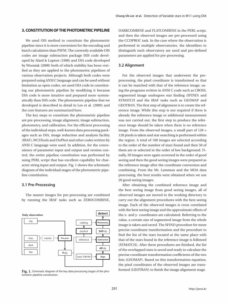
acter string input and output. Fig. 1 shows the schematic

diagram of the individual stages of the photometric pipe-

line constitution.

3.1 Pre-Processing

The master images for pre-processing are combined

by running the IRAF tasks such as ZEROCOMBINE,

DARKCOMBINE and FLATCOMBINE in the PERL script,

and then the observed images are pre-processed using

the CCDPROC task. In the case where the observation is

performed in multiple observatories, the identifiers to

distinguish each observatory are used and pre-defined

parameters are applied for pre-processing.

3.2 Alignment

For the observed images that underwent the pre-

processing, the pixel coordinate is transformed so that

it can be matched with that of the reference image, us-

ing the programs written in ANSI C code such as CROSS,

segmented image undergoes star finding (SFIND) and

XYMATCH and the IRAF tasks such as GEOMAP and

GEOTRAN. The first step of alignment is to create the ref-

erence image. While this step is not required if there is

already the reference image or additional measurement

was not carried out, the first step to produce the refer-

ence image should be taken when there is no reference

image. From the observed images, a small part of 128 ×

128 pixels is taken and star searching is performed within

the region. A total of 100 images are selected according

to the order of the number of stars found and then 50 of

them are re-selected in the order of low background. Fi-

nally, 20 images were again screened in the order of good

seeing and then the good seeing images were prepared as

the reference image after the coordinate conversion and

combining. From the Mt. Lemmon and the MOA data

processing, the best results were obtained when we use

20 good seeing images.

After obtaining the combined reference image and

the best seeing image from good seeing images, all of

observed images are moved to the working directory to

carry out the alignment procedures with the best seeing

image. Each of the observed images is cross correlated

with the best seeing image and the approximate offsets of

the x- and y- coordinates are calculated. Referring to the

value, a certain size of segmented image from the whole

image is taken and saved. The SFIND procedure for more

precise coordinate transformation and the procedure to

find the list of the stars located at the same place with

that of the stars found in the reference image is followed

(XYMATCH). After these procedures are finished, the list

of the overlapped stars is saved and ready to calculate the

precise coordinate transformation coefficients of the two

lists (GEOMAP). Based on this transformation equation,

the pixel coordinates of the observed images are trans-

formed (GEOTRAN) to finish the image alignment stage.Fig. 1. Schematic diagram of the key data-processing stages of the pho-tometric pipeline constitution.

DOI: 10.5140/JASS.2010.27.4.289 292


3.3 Image Subtraction

We modified the DIA code that was developed by Woz-

niak (2000) to use it for the image subtraction engine. As

described in Section 2, the convolution kernel is obtained

through OIS using the observed images and the reference

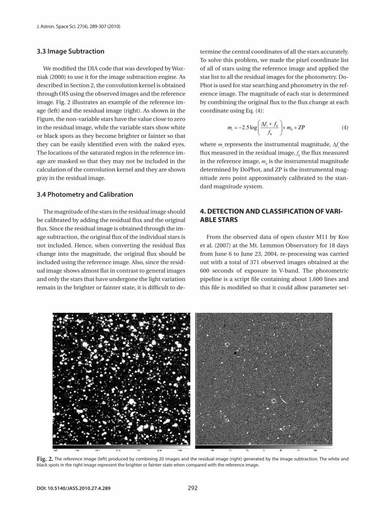
image. Fig. 2 illustrates an example of the reference im-

age (left) and the residual image (right). As shown in the

Figure, the non-variable stars have the value close to zero

in the residual image, while the variable stars show white

or black spots as they become brighter or fainter so that

they can be easily identified even with the naked eyes.

The locations of the saturated region in the reference im-

age are masked so that they may not be included in the

calculation of the convolution kernel and they are shown

gray in the residual image.

3.4 Photometry and Calibration

The magnitude of the stars in the residual image should

be calibrated by adding the residual flux and the original

flux. Since the residual image is obtained through the im-

age subtraction, the original flux of the individual stars is

not included. Hence, when converting the residual flux

change into the magnitude, the original flux should be

included using the reference image. Also, since the resid-

ual image shows almost flat in contrast to general images

and only the stars that have undergone the light variation

remain in the brighter or fainter state, it is difficult to de-

termine the central coordinates of all the stars accurately.

To solve this problem, we made the pixel coordinate list

of all of stars using the reference image and applied the

star list to all the residual images for the photometry. Do-

Phot is used for star searching and photometry in the ref-

erence image. The magnitude of each star is determined

by combining the original flux to the flux change at each

coordinate using Eq. (4):

00

0

2.5log ZPii

f fm mf

∆ += − + +

(4)

where mi represents the instrumental magnitude, ∆fi the

flux measured in the residual image, f0 the flux measured

in the reference image, m0 is the instrumental magnitude

determined by DoPhot, and ZP is the instrumental mag-

nitude zero point approximately calibrated to the stan-

dard magnitude system.

4. DETECTION AND CLASSIFICATION OF VARI-ABLE STARS

From the observed data of open cluster M11 by Koo

et al. (2007) at the Mt. Lemmon Observatory for 18 days

from June 6 to June 23, 2004, re-processing was carried

out with a total of 371 observed images obtained at the

600 seconds of exposure in V-band. The photometric

pipeline is a script file containing about 1,600 lines and

this file is modified so that it could allow parameter set-

Fig. 2. The reference image (left) produced by combining 20 images and the residual image (right) generated by the image subtraction. The white and black spots in the right image represent the brighter or fainter state when compared with the reference image.

293


http://janss.kr

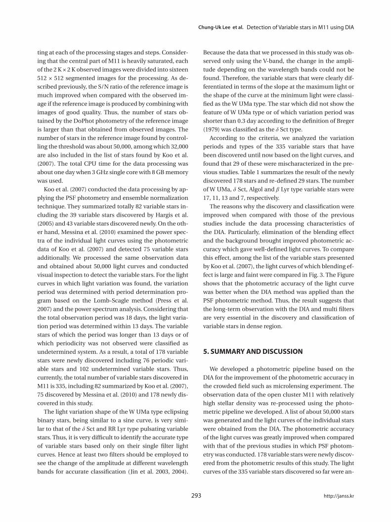
ting at each of the processing stages and steps. Consider-

ing that the central part of M11 is heavily saturated, each

of the 2 K × 2 K observed images were divided into sixteen

512 × 512 segmented images for the processing. As de-

scribed previously, the S/N ratio of the reference image is

much improved when compared with the observed im-

age if the reference image is produced by combining with

images of good quality. Thus, the number of stars ob-

tained by the DoPhot photometry of the reference image

is larger than that obtained from observed images. The

number of stars in the reference image found by control-

ling the threshold was about 50,000, among which 32,000

are also included in the list of stars found by Koo et al.

(2007). The total CPU time for the data processing was

about one day when 3 GHz single core with 8 GB memory

was used.

Koo et al. (2007) conducted the data processing by ap-

plying the PSF photometry and ensemble normalization

technique. They summarized totally 82 variable stars in-

cluding the 39 variable stars discovered by Hargis et al.

(2005) and 43 variable stars discovered newly. On the oth-

er hand, Messina et al. (2010) examined the power spec-

tra of the individual light curves using the photometric

data of Koo et al. (2007) and detected 75 variable stars

additionally. We processed the same observation data

and obtained about 50,000 light curves and conducted

visual inspection to detect the variable stars. For the light

curves in which light variation was found, the variation

period was determined with period determination pro-

gram based on the Lomb-Scagle method (Press et al.

2007) and the power spectrum analysis. Considering that

the total observation period was 18 days, the light varia-

tion period was determined within 13 days. The variable

stars of which the period was longer than 13 days or of

which periodicity was not observed were classified as

undetermined system. As a result, a total of 178 variable

stars were newly discovered including 76 periodic vari-

able stars and 102 undetermined variable stars. Thus,

currently, the total number of variable stars discovered in

M11 is 335, including 82 summarized by Koo et al. (2007),

75 discovered by Messina et al. (2010) and 178 newly dis-

covered in this study.

The light variation shape of the W UMa type eclipsing

binary stars, being similar to a sine curve, is very simi-

lar to that of the δ Sct and RR Lyr type pulsating variable

stars. Thus, it is very difficult to identify the accurate type

of variable stars based only on their single filter light

curves. Hence at least two filters should be employed to

see the change of the amplitude at different wavelength

bands for accurate classification (Jin et al. 2003, 2004).

Because the data that we processed in this study was ob-

served only using the V-band, the change in the ampli-

tude depending on the wavelength bands could not be

found. Therefore, the variable stars that were clearly dif-

ferentiated in terms of the slope at the maximum light or

the shape of the curve at the minimum light were classi-

fied as the W UMa type. The star which did not show the

feature of W UMa type or of which variation period was

shorter than 0.3 day according to the definition of Breger

(1979) was classified as the δ Sct type.

According to the criteria, we analyzed the variation

periods and types of the 335 variable stars that have

been discovered until now based on the light curves, and

found that 29 of these were mischaracterized in the pre-

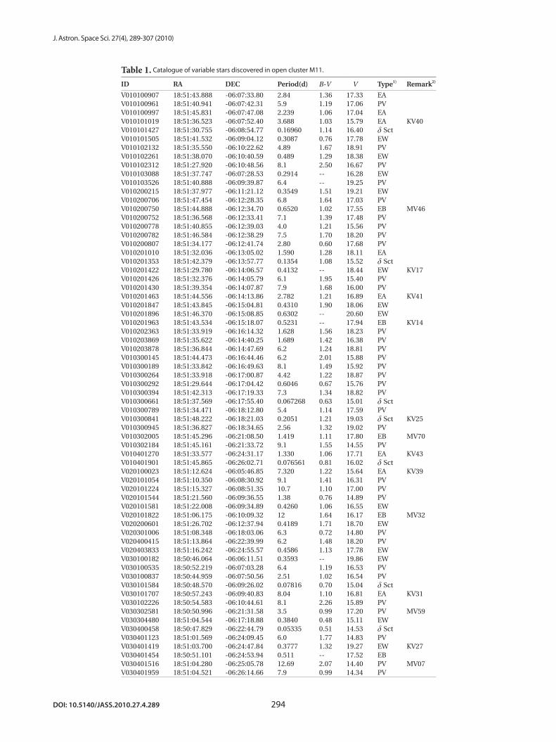
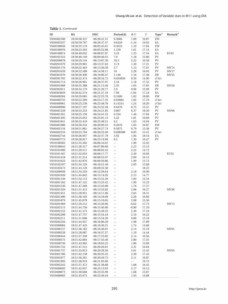
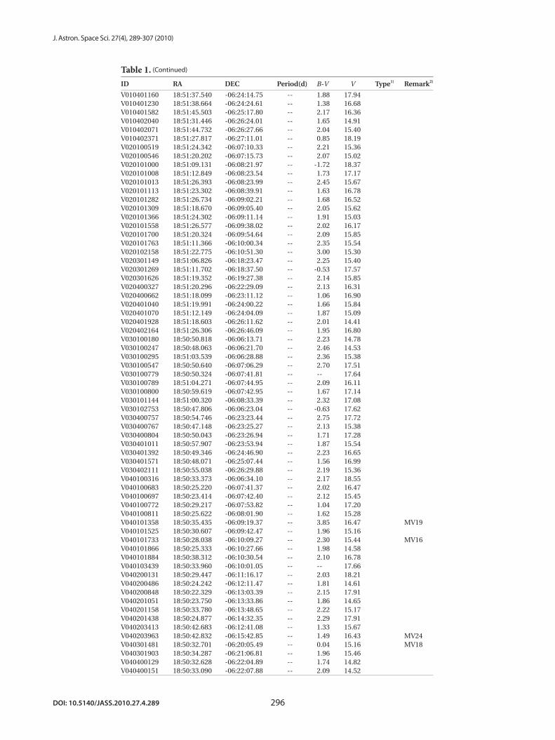
vious studies. Table 1 summarizes the result of the newly

discovered 178 stars and re-defined 29 stars. The number

of W UMa, δ Sct, Algol and β Lyr type variable stars were

17, 11, 13 and 7, respectively.

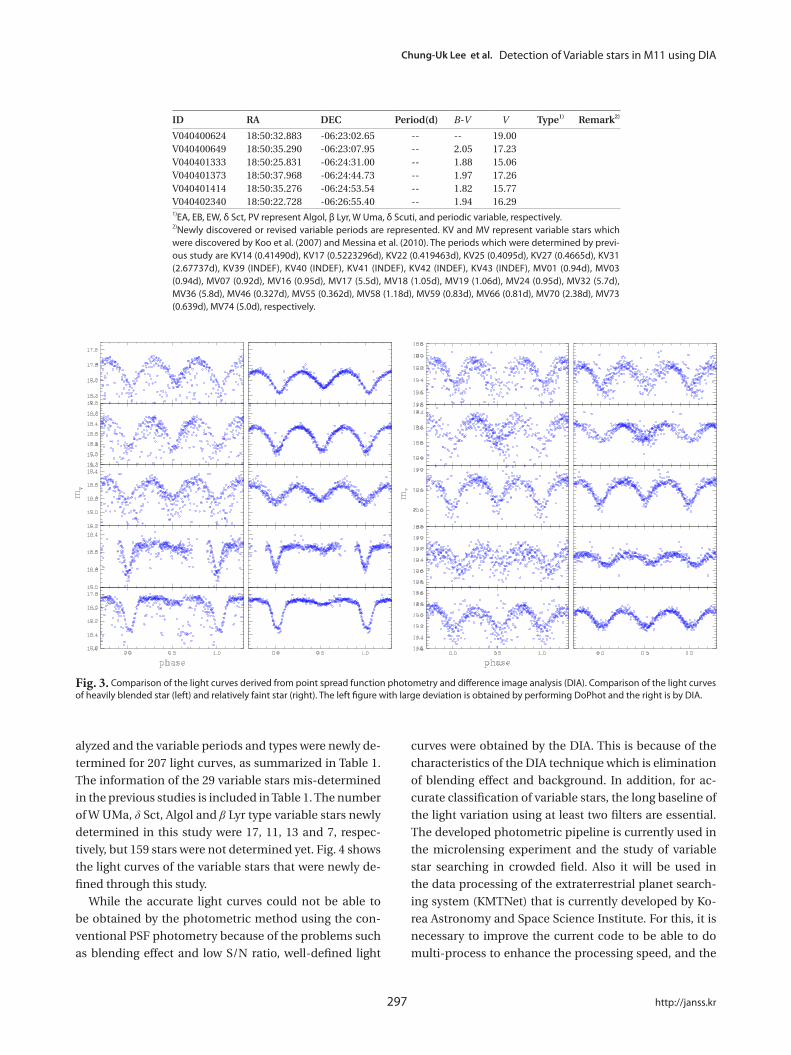
The reasons why the discovery and classification were

improved when compared with those of the previous

studies include the data processing characteristics of

the DIA. Particularly, elimination of the blending effect

and the background brought improved photometric ac-

curacy which gave well-defined light curves. To compare

this effect, among the list of the variable stars presented

by Koo et al. (2007), the light curves of which blending ef-

fect is large and faint were compared in Fig. 3. The Figure

shows that the photometric accuracy of the light curve

was better when the DIA method was applied than the

PSF photometric method. Thus, the result suggests that

the long-term observation with the DIA and multi filters

are very essential in the discovery and classification of

variable stars in dense region.

5. SUMMARY AND DISCUSSION

We developed a photometric pipeline based on the

DIA for the improvement of the photometric accuracy in

the crowded field such as microlensing experiment. The

observation data of the open cluster M11 with relatively

high stellar density was re-processed using the photo-

metric pipeline we developed. A list of about 50,000 stars

was generated and the light curves of the individual stars

were obtained from the DIA. The photometric accuracy

of the light curves was greatly improved when compared

with that of the previous studies in which PSF photom-

etry was conducted. 178 variable stars were newly discov-

ered from the photometric results of this study. The light

curves of the 335 variable stars discovered so far were an-

DOI: 10.5140/JASS.2010.27.4.289 294


Table 1. Catalogue of variable stars discovered in open cluster M11.

ID RA DEC Period(d) B-V V Type1) Remark2)

V010100907 18:51:43.888 -06:07:33.80 2.84 1.36 17.33 EAV010100961 18:51:40.941 -06:07:42.31 5.9 1.19 17.06 PVV010100997 18:51:45.831 -06:07:47.08 2.239 1.06 17.04 EAV010101019 18:51:36.523 -06:07:52.40 3.688 1.03 15.79 EA KV40V010101427 18:51:30.755 -06:08:54.77 0.16960 1.14 16.40 δ SctV010101505 18:51:41.532 -06:09:04.12 0.3087 0.76 17.78 EWV010102132 18:51:35.550 -06:10:22.62 4.89 1.67 18.91 PVV010102261 18:51:38.070 -06:10:40.59 0.489 1.29 18.38 EWV010102312 18:51:27.920 -06:10:48.56 8.1 2.50 16.67 PVV010103088 18:51:37.747 -06:07:28.53 0.2914 -- 16.28 EWV010103526 18:51:40.888 -06:09:39.87 6.4 -- 19.25 PVV010200215 18:51:37.977 -06:11:21.12 0.3549 1.51 19.21 EWV010200706 18:51:47.454 -06:12:28.35 6.8 1.64 17.03 PVV010200750 18:51:44.888 -06:12:34.70 0.6520 1.02 17.55 EB MV46V010200752 18:51:36.568 -06:12:33.41 7.1 1.39 17.48 PVV010200778 18:51:40.855 -06:12:39.03 4.0 1.21 15.56 PVV010200782 18:51:46.584 -06:12:38.29 7.5 1.70 18.20 PVV010200807 18:51:34.177 -06:12:41.74 2.80 0.60 17.68 PVV010201010 18:51:32.036 -06:13:05.02 1.590 1.28 18.11 EAV010201353 18:51:42.379 -06:13:57.77 0.1354 1.08 15.52 δ SctV010201422 18:51:29.780 -06:14:06.57 0.4132 -- 18.44 EW KV17V010201426 18:51:32.376 -06:14:05.79 6.1 1.95 15.40 PVV010201430 18:51:39.354 -06:14:07.87 7.9 1.68 16.00 PVV010201463 18:51:44.556 -06:14:13.86 2.782 1.21 16.89 EA KV41V010201847 18:51:43.845 -06:15:04.81 0.4310 1.90 18.06 EWV010201896 18:51:46.370 -06:15:08.85 0.6302 -- 20.60 EWV010201963 18:51:43.534 -06:15:18.07 0.5231 -- 17.94 EB KV14V010202363 18:51:33.919 -06:16:14.32 1.628 1.56 18.23 PVV010203869 18:51:35.622 -06:14:40.25 1.689 1.42 16.38 PVV010203878 18:51:36.844 -06:14:47.69 6.2 1.24 18.81 PVV010300145 18:51:44.473 -06:16:44.46 6.2 2.01 15.88 PVV010300189 18:51:33.842 -06:16:49.63 8.1 1.49 15.92 PVV010300264 18:51:33.918 -06:17:00.87 4.42 1.22 18.87 PVV010300292 18:51:29.644 -06:17:04.42 0.6046 0.67 15.76 PVV010300394 18:51:42.313 -06:17:19.33 7.3 1.34 18.82 PVV010300661 18:51:37.569 -06:17:55.40 0.067268 0.63 15.01 δ SctV010300789 18:51:34.471 -06:18:12.80 5.4 1.14 17.59 PVV010300841 18:51:48.222 -06:18:21.03 0.2051 1.21 19.03 δ Sct KV25V010300945 18:51:36.827 -06:18:34.65 2.56 1.32 19.02 PVV010302005 18:51:45.296 -06:21:08.50 1.419 1.11 17.80 EB MV70V010302184 18:51:45.161 -06:21:33.72 9.1 1.55 14.55 PVV010401270 18:51:33.577 -06:24:31.17 1.330 1.06 17.71 EA KV43V010401901 18:51:45.865 -06:26:02.71 0.076561 0.81 16.02 δ SctV020100023 18:51:12.624 -06:05:46.85 7.320 1.22 15.64 EA KV39V020101054 18:51:10.350 -06:08:30.92 9.1 1.41 16.31 PVV020101224 18:51:15.327 -06:08:51.35 10.7 1.10 17.00 PVV020101544 18:51:21.560 -06:09:36.55 1.38 0.76 14.89 PVV020101581 18:51:22.008 -06:09:34.89 0.4260 1.06 16.55 EWV020101822 18:51:06.175 -06:10:09.32 12 1.64 16.17 EB MV32V020200601 18:51:26.702 -06:12:37.94 0.4189 1.71 18.70 EWV020301006 18:51:08.348 -06:18:03.06 6.3 0.72 14.80 PVV020400415 18:51:13.864 -06:22:39.99 6.2 1.48 18.20 PVV020403833 18:51:16.242 -06:24:55.57 0.4586 1.13 17.78 EWV030100182 18:50:46.064 -06:06:11.51 0.3593 -- 19.86 EWV030100535 18:50:52.219 -06:07:03.28 6.4 1.19 16.53 PVV030100837 18:50:44.959 -06:07:50.56 2.51 1.02 16.54 PVV030101584 18:50:48.570 -06:09:26.02 0.07816 0.70 15.04 δ SctV030101707 18:50:57.243 -06:09:40.83 8.04 1.10 16.81 EA KV31V030102226 18:50:54.583 -06:10:44.61 8.1 2.26 15.89 PVV030302581 18:50:50.996 -06:21:31.58 3.5 0.99 17.20 PV MV59V030304480 18:51:04.544 -06:17:18.88 0.3840 0.48 15.11 EW V030400458 18:50:47.829 -06:22:44.79 0.05335 0.51 14.53 δ SctV030401123 18:51:01.569 -06:24:09.45 6.0 1.77 14.83 PV V030401419 18:51:03.700 -06:24:47.84 0.3777 1.32 19.27 EW KV27V030401454 18:50:51.101 -06:24:53.94 0.511 -- 17.52 EB V030401516 18:51:04.280 -06:25:05.78 12.69 2.07 14.40 PV MV07V030401959 18:51:04.521 -06:26:14.66 7.9 0.99 14.34 PV

295


http://janss.kr

Table 1. (Continued)


V030402180 18:50:58.337 -06:26:41.31 0.3666 1.09 16.87 EW V030403337 18:50:59.797 -06:26:37.47 0.6329 -1.34 19.03 EA V040100050 18:50:33.119 -06:05:45.61 0.3616 1.10 17.84 EW V040100076 18:50:23.293 -06:05:52.88 1.159 1.01 17.14 EA V040100874 18:50:40.632 -06:08:07.07 3.53 1.23 17.54 EA KV42V040101523 18:50:40.149 -06:09:40.55 7.9 1.18 15.86 PV V040200878 18:50:29.134 -06:13:07.50 10.3 2.22 16.58 PV V040201079 18:50:29.901 -06:13:37.62 11.9 1.30 17.21 PV V040201176 18:50:22.463 -06:13:50.50 5.7 1.13 17.61 PV MV74V040201639 18:50:32.588 -06:14:58.11 10 2.28 16.05 PV MV17V040301070 18:50:30.490 -06:19:06.47 1.146 1.16 17.48 EB MV55V040301702 18:50:22.474 -06:20:34.75 0.034830 0.56 14.90 δ SctV040301714 18:50:26.901 -06:20:37.97 2.34 1.18 17.52 PV V040301968 18:50:35.388 -06:21:13.46 2.35 1.05 17.65 EB MV58V040302011 18:50:34.179 -06:21:20.77 5.9 0.96 15.99 PV V040303859 18:50:42.274 -06:21:27.19 7.99 -1.04 17.24 EA V040400304 18:50:29.065 -06:22:25.78 0.3400 1.62 18.80 EW V040400735 18:50:22.509 -06:23:17.35 0.03684 1.02 17.19 δ SctV040400961 18:50:25.238 -06:23:48.76 0.14314 1.24 18.20 δ SctV040400990 18:50:27.197 -06:23:52.58 0.6470 0.75 15.51 PV V040401228 18:50:33.253 -06:24:21.85 0.807 0.37 18.50 PV MV66V040401361 18:50:25.150 -06:24:41.55 0.334 1.46 17.84 PV V040401495 18:50:25.053 -06:25:01.13 5.42 1.01 16.69 PV V040401841 18:50:32.410 -06:25:48.51 6.2 1.63 14.94 PV V040401980 18:50:30.234 -06:26:09.52 0.2676 1.65 16.87 EW V040402134 18:50:31.861 -06:26:27.74 0.5875 0.79 15.38 PV V040402310 18:50:33.764 -06:26:53.40 0.098388 0.85 15.41 δ SctV040402744 18:50:26.957 -06:22:37.78 3.92 1.84 18.54 EA V040403773 18:50:28.817 -06:25:19.98 8.2 1.30 16.47 PV V010100305 18:51:35.502 -06:06:16.01 -- 1.99 15.92V010100643 18:51:28.317 -06:07:00.66 -- 2.23 15.13V010101090 18:51:29.511 -06:08:03.43 -- 2.22 14.72V010101187 18:51:32.053 -06:08:17.77 -- 2.49 16.69 KV22V010101418 18:51:31.214 -06:08:53.97 -- 2.09 16.15V010101623 18:51:42.876 -06:09:20.86 -- 1.99 15.73V010102107 18:51:34.129 -06:10:21.49 -- 2.05 15.68V010103473 18:51:43.129 -06:09:22.38 -- -- 18.22V010200938 18:51:34.310 -06:12:59.64 -- 2.18 16.90V010201039 18:51:44.842 -06:13:14.95 -- 2.13 14.77V010201156 18:51:32.113 -06:13:32.29 -- 1.84 15.54V010201162 18:51:47.122 -06:13:33.42 -- 1.90 15.23V010201236 18:51:47.569 -06:13:43.08 -- 1.76 17.37V010201329 18:51:31.412 -06:13:53.82 -- 2.06 16.27 MV36V010201451 18:51:28.951 -06:14:11.60 -- 2.65 18.31V010201486 18:51:38.103 -06:14:16.69 -- 2.26 16.66V010201879 18:51:45.078 -06:15:10.85 -- 2.08 15.56V010201969 18:51:29.212 -06:15:20.96 -- -0.62 17.73 MV73V010202113 18:51:44.750 -06:15:40.90 -- -0.90 17.10V010202152 18:51:41.575 -06:15:49.32 -- 2.49 17.10V010202208 18:51:47.757 -06:15:54.44 -- 2.16 16.22V010202211 18:51:31.606 -06:15:54.36 -- 0.80 15.18V010202256 18:51:44.937 -06:16:00.20 -- 1.98 17.89V010300084 18:51:47.445 -06:16:36.51 -- 1.74 14.68V010300127 18:51:36.182 -06:16:40.91 -- 2.14 15.19 MV01V010300228 18:51:28.087 -06:16:57.27 -- 1.19 14.44V010300444 18:51:37.358 -06:17:25.82 -- 2.14 16.56V010300575 18:51:42.684 -06:17:43.46 -- 2.80 17.35V010300730 18:51:43.963 -06:18:05.25 -- 1.86 15.09V010301732 18:51:47.315 -06:20:26.61 -- 2.31 16.04V010301737 18:51:33.813 -06:20:28.56 -- 2.01 15.42 MV03V010301786 18:51:42.158 -06:20:35.35 -- 2.30 17.45V010301877 18:51:36.201 -06:20:49.73 -- 2.11 16.87V010301995 18:51:28.919 -06:21:03.00 -- -- 19.73V010302245 18:51:37.472 -06:21:38.68 -- 1.68 16.45V010400695 18:51:42.037 -06:23:13.03 -- 2.17 16.15V010400873 18:51:30.668 -06:23:35.99 -- 1.68 15.87V010400965 18:51:45.673 -06:23:49.44 -- 1.93 14.88

DOI: 10.5140/JASS.2010.27.4.289 296


Table 1. (Continued)


V010401160 18:51:37.540 -06:24:14.75 -- 1.88 17.94V010401230 18:51:38.664 -06:24:24.61 -- 1.38 16.68V010401582 18:51:45.503 -06:25:17.80 -- 2.17 16.36V010402040 18:51:31.446 -06:26:24.01 -- 1.65 14.91V010402071 18:51:44.732 -06:26:27.66 -- 2.04 15.40V010402371 18:51:27.817 -06:27:11.01 -- 0.85 18.19V020100519 18:51:24.342 -06:07:10.33 -- 2.21 15.36V020100546 18:51:20.202 -06:07:15.73 -- 2.07 15.02V020101000 18:51:09.131 -06:08:21.97 -- -1.72 18.37V020101008 18:51:12.849 -06:08:23.54 -- 1.73 17.17V020101013 18:51:26.393 -06:08:23.99 -- 2.45 15.67V020101113 18:51:23.302 -06:08:39.91 -- 1.63 16.78V020101282 18:51:26.734 -06:09:02.21 -- 1.68 16.52V020101309 18:51:18.670 -06:09:05.40 -- 2.05 15.62V020101366 18:51:24.302 -06:09:11.14 -- 1.91 15.03V020101558 18:51:26.577 -06:09:38.02 -- 2.02 16.17V020101700 18:51:20.324 -06:09:54.64 -- 2.09 15.85V020101763 18:51:11.366 -06:10:00.34 -- 2.35 15.54V020102158 18:51:22.775 -06:10:51.30 -- 3.00 15.30V020301149 18:51:06.826 -06:18:23.47 -- 2.25 15.40V020301269 18:51:11.702 -06:18:37.50 -- -0.53 17.57V020301626 18:51:19.352 -06:19:27.38 -- 2.14 15.85V020400327 18:51:20.296 -06:22:29.09 -- 2.13 16.31V020400662 18:51:18.099 -06:23:11.12 -- 1.06 16.90V020401040 18:51:19.991 -06:24:00.22 -- 1.66 15.84V020401070 18:51:12.149 -06:24:04.09 -- 1.87 15.09V020401928 18:51:18.603 -06:26:11.62 -- 2.01 14.41V020402164 18:51:26.306 -06:26:46.09 -- 1.95 16.80V030100180 18:50:50.818 -06:06:13.71 -- 2.23 14.78V030100247 18:50:48.063 -06:06:21.70 -- 2.46 14.53V030100295 18:51:03.539 -06:06:28.88 -- 2.36 15.38V030100547 18:50:50.640 -06:07:06.29 -- 2.70 17.51V030100779 18:50:50.324 -06:07:41.81 -- -- 17.64V030100789 18:51:04.271 -06:07:44.95 -- 2.09 16.11V030100800 18:50:59.619 -06:07:42.95 -- 1.67 17.14V030101144 18:51:00.320 -06:08:33.39 -- 2.32 17.08V030102753 18:50:47.806 -06:06:23.04 -- -0.63 17.62V030400757 18:50:54.746 -06:23:23.44 -- 2.75 17.72V030400767 18:50:47.148 -06:23:25.27 -- 2.13 15.38V030400804 18:50:50.043 -06:23:26.94 -- 1.71 17.28V030401011 18:50:57.907 -06:23:53.94 -- 1.87 15.54V030401392 18:50:49.346 -06:24:46.90 -- 2.23 16.65V030401571 18:50:48.071 -06:25:07.44 -- 1.56 16.99V030402111 18:50:55.038 -06:26:29.88 -- 2.19 15.36V040100316 18:50:33.373 -06:06:34.10 -- 2.17 18.55V040100683 18:50:25.220 -06:07:41.37 -- 2.02 16.47V040100697 18:50:23.414 -06:07:42.40 -- 2.12 15.45V040100772 18:50:29.217 -06:07:53.82 -- 1.04 17.20V040100811 18:50:25.622 -06:08:01.90 -- 1.62 15.28V040101358 18:50:35.435 -06:09:19.37 -- 3.85 16.47 MV19V040101525 18:50:30.607 -06:09:42.47 -- 1.96 15.16V040101733 18:50:28.038 -06:10:09.27 -- 2.30 15.44 MV16V040101866 18:50:25.333 -06:10:27.66 -- 1.98 14.58V040101884 18:50:38.312 -06:10:30.54 -- 2.10 16.78V040103439 18:50:33.960 -06:10:01.05 -- -- 17.66V040200131 18:50:29.447 -06:11:16.17 -- 2.03 18.21V040200486 18:50:24.242 -06:12:11.47 -- 1.81 14.61V040200848 18:50:22.329 -06:13:03.39 -- 2.15 17.91V040201051 18:50:23.750 -06:13:33.86 -- 1.86 14.65V040201158 18:50:33.780 -06:13:48.65 -- 2.22 15.17V040201438 18:50:24.877 -06:14:32.35 -- 2.29 17.91V040203413 18:50:42.683 -06:12:41.08 -- 1.33 15.67V040203963 18:50:42.832 -06:15:42.85 -- 1.49 16.43 MV24V040301481 18:50:32.701 -06:20:05.49 -- 0.04 15.16 MV18V040301903 18:50:34.287 -06:21:06.81 -- 1.96 15.46V040400129 18:50:32.628 -06:22:04.89 -- 1.74 14.82V040400151 18:50:33.090 -06:22:07.88 -- 2.09 14.52

297


http://janss.kr

Fig. 3. Comparison of the light curves derived from point spread function photometry and difference image analysis (DIA). Comparison of the light curves of heavily blended star (left) and relatively faint star (right). The left figure with large deviation is obtained by performing DoPhot and the right is by DIA.

alyzed and the variable periods and types were newly de-

termined for 207 light curves, as summarized in Table 1.

The information of the 29 variable stars mis-determined

in the previous studies is included in Table 1. The number

of W UMa, δ Sct, Algol and β Lyr type variable stars newly

determined in this study were 17, 11, 13 and 7, respec-

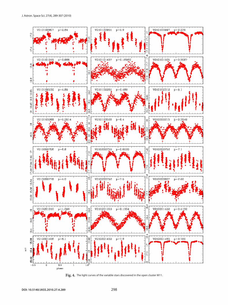
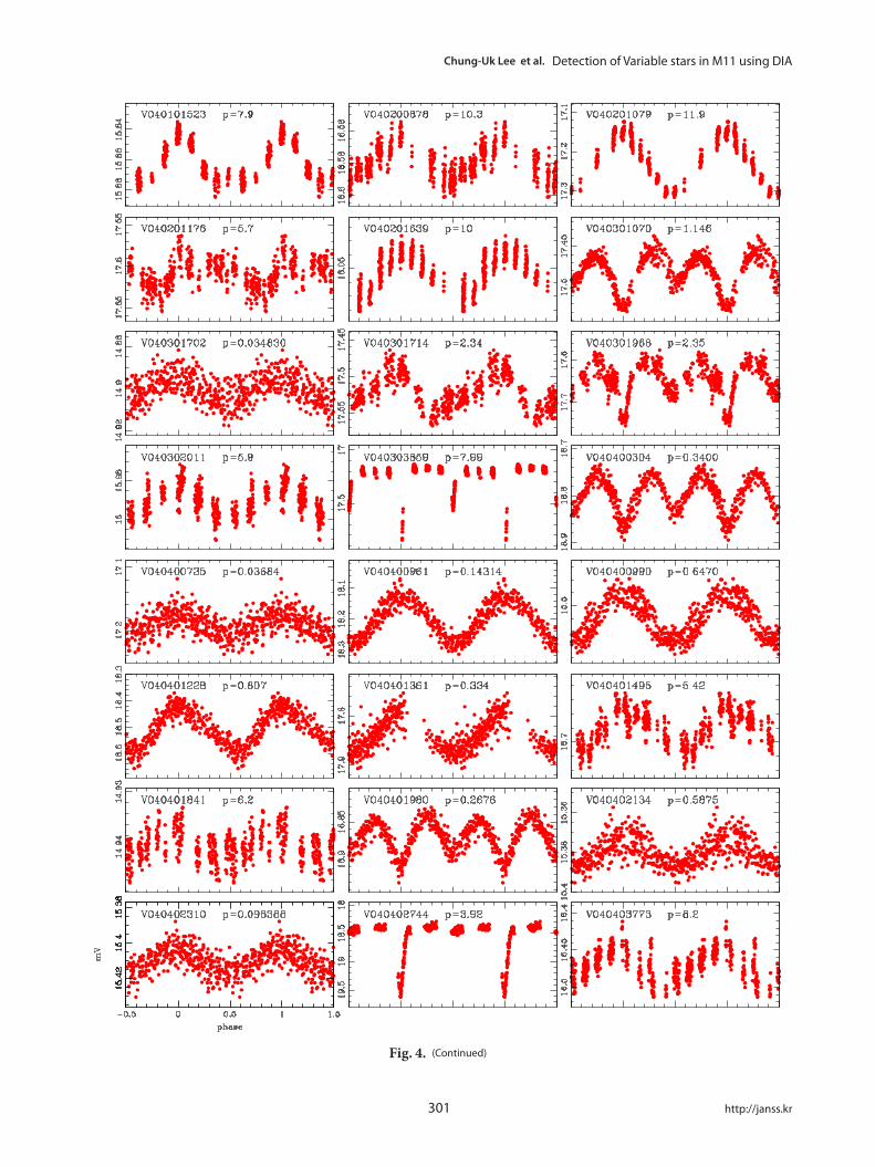
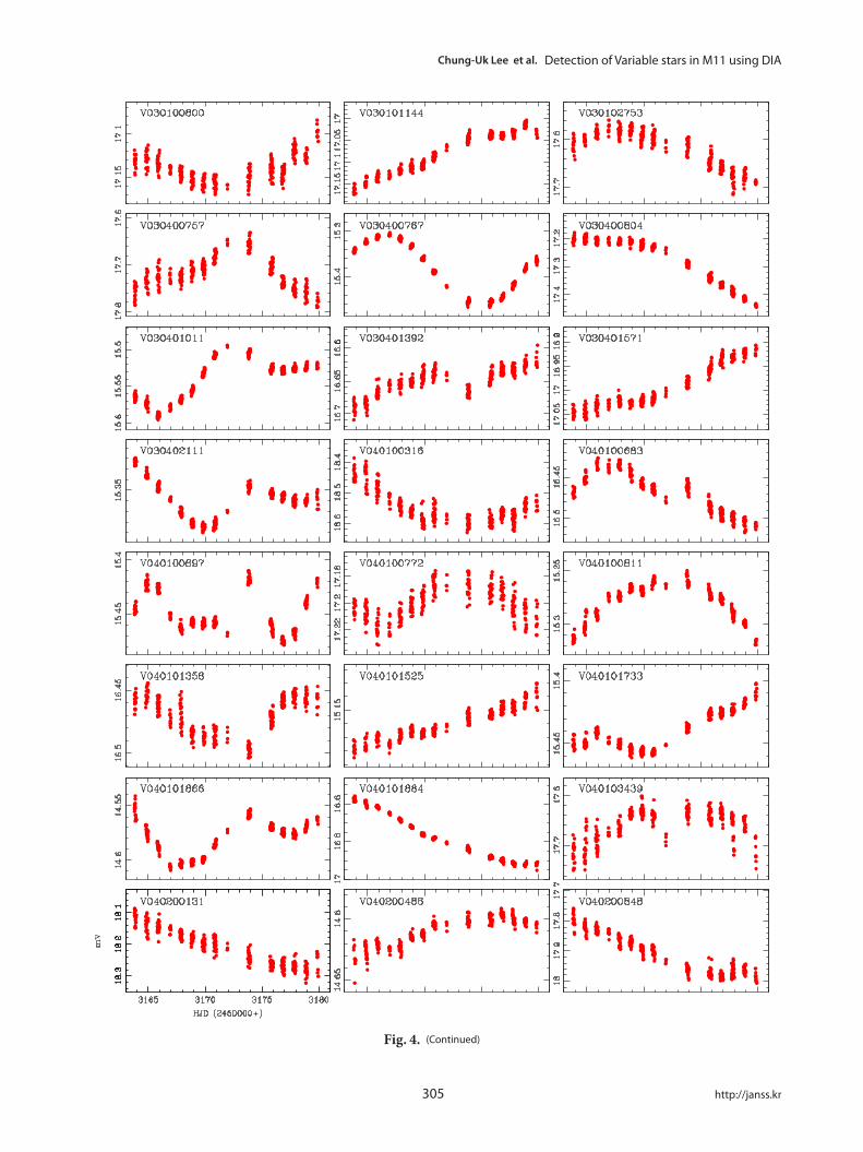
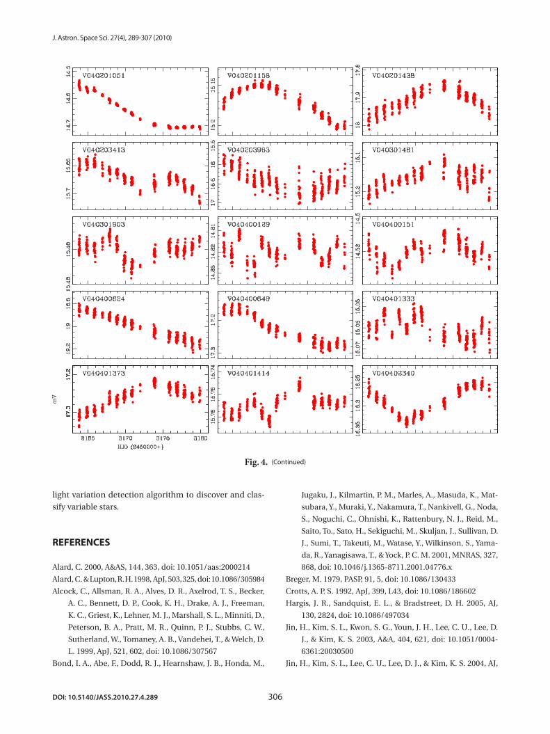
tively, but 159 stars were not determined yet. Fig. 4 shows

the light curves of the variable stars that were newly de-

fined through this study.

While the accurate light curves could not be able to

be obtained by the photometric method using the con-

ventional PSF photometry because of the problems such

as blending effect and low S/N ratio, well-defined light


V040400624 18:50:32.883 -06:23:02.65 -- -- 19.00V040400649 18:50:35.290 -06:23:07.95 -- 2.05 17.23V040401333 18:50:25.831 -06:24:31.00 -- 1.88 15.06V040401373 18:50:37.968 -06:24:44.73 -- 1.97 17.26V040401414 18:50:35.276 -06:24:53.54 -- 1.82 15.77V040402340 18:50:22.728 -06:26:55.40 -- 1.94 16.291)EA, EB, EW, δ Sct, PV represent Algol, β Lyr, W Uma, δ Scuti, and periodic variable, respectively.2)Newly discovered or revised variable periods are represented. KV and MV represent variable stars which were discovered by Koo et al. (2007) and Messina et al. (2010). The periods which were determined by previ-ous study are KV14 (0.41490d), KV17 (0.5223296d), KV22 (0.419463d), KV25 (0.4095d), KV27 (0.4665d), KV31 (2.67737d), KV39 (INDEF), KV40 (INDEF), KV41 (INDEF), KV42 (INDEF), KV43 (INDEF), MV01 (0.94d), MV03 (0.94d), MV07 (0.92d), MV16 (0.95d), MV17 (5.5d), MV18 (1.05d), MV19 (1.06d), MV24 (0.95d), MV32 (5.7d), MV36 (5.8d), MV46 (0.327d), MV55 (0.362d), MV58 (1.18d), MV59 (0.83d), MV66 (0.81d), MV70 (2.38d), MV73 (0.639d), MV74 (5.0d), respectively.

curves were obtained by the DIA. This is because of the

characteristics of the DIA technique which is elimination

of blending effect and background. In addition, for ac-

curate classification of variable stars, the long baseline of

the light variation using at least two filters are essential.

The developed photometric pipeline is currently used in

the microlensing experiment and the study of variable

star searching in crowded field. Also it will be used in

the data processing of the extraterrestrial planet search-

ing system (KMTNet) that is currently developed by Ko-

rea Astronomy and Space Science Institute. For this, it is

necessary to improve the current code to be able to do

multi-process to enhance the processing speed, and the

DOI: 10.5140/JASS.2010.27.4.289 298


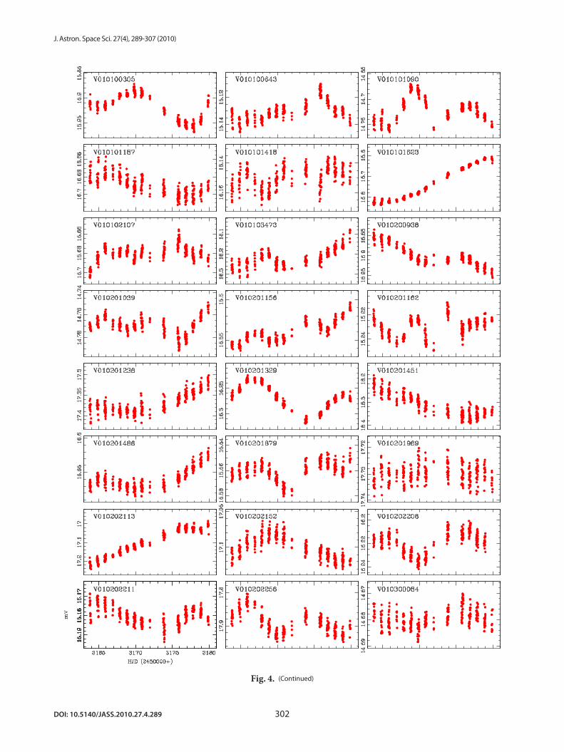
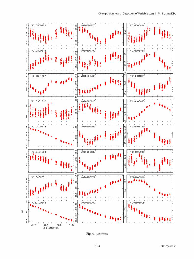
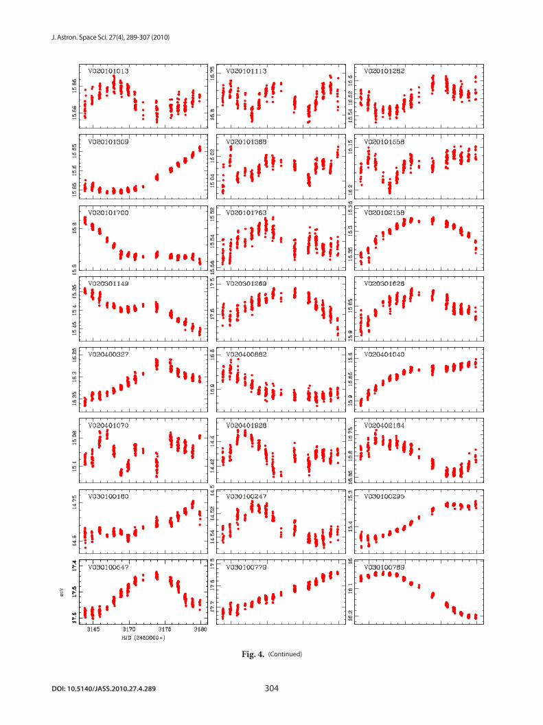
Fig. 4. The light curves of the variable stars discovered in the open cluster M11.

299


http://janss.kr

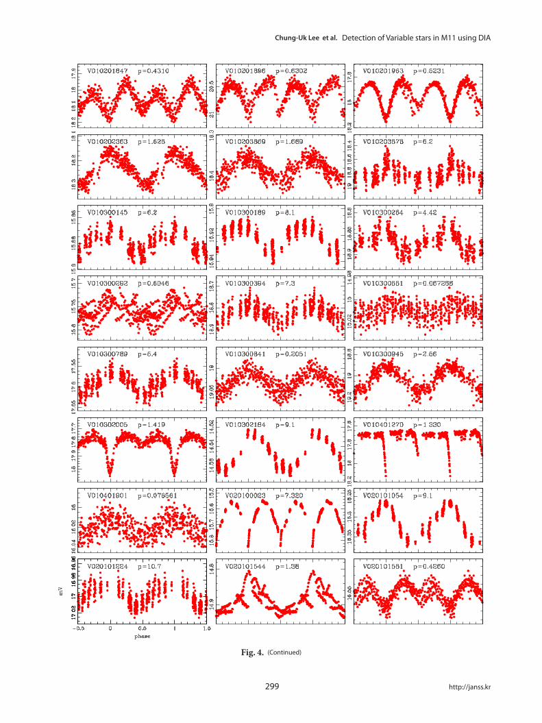
Fig. 4. (Continued)

DOI: 10.5140/JASS.2010.27.4.289 300


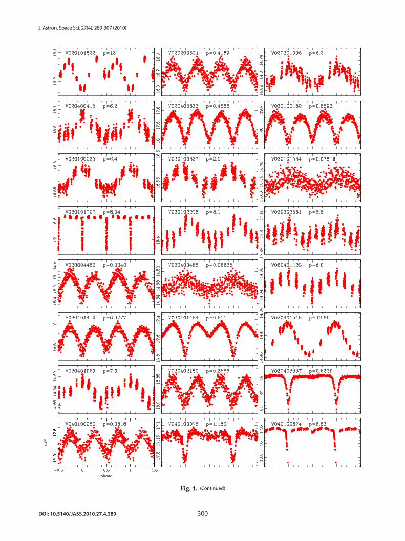
Fig. 4. (Continued)

301


http://janss.kr

Fig. 4. (Continued)

DOI: 10.5140/JASS.2010.27.4.289 302


Fig. 4. (Continued)

303


http://janss.kr

Fig. 4. (Continued)

DOI: 10.5140/JASS.2010.27.4.289 304


Fig. 4. (Continued)

305


http://janss.kr

Fig. 4. (Continued)

DOI: 10.5140/JASS.2010.27.4.289 306


light variation detection algorithm to discover and clas-

sify variable stars.

REFERENCES

Alard, C. 2000, A&AS, 144, 363, doi: 10.1051/aas:2000214

Alard, C. & Lupton, R. H. 1998, ApJ, 503, 325, doi: 10.1086/305984

Alcock, C., Allsman, R. A., Alves, D. R., Axelrod, T. S., Becker,

A. C., Bennett, D. P., Cook, K. H., Drake, A. J., Freeman,

K. C., Griest, K., Lehner, M. J., Marshall, S. L., Minniti, D.,

Peterson, B. A., Pratt, M. R., Quinn, P. J., Stubbs, C. W.,

Sutherland, W., Tomaney, A. B., Vandehei, T., & Welch, D.

L. 1999, ApJ, 521, 602, doi: 10.1086/307567

Bond, I. A., Abe, F., Dodd, R. J., Hearnshaw, J. B., Honda, M.,

Jugaku, J., Kilmartin, P. M., Marles, A., Masuda, K., Mat-

subara, Y., Muraki, Y., Nakamura, T., Nankivell, G., Noda,

S., Noguchi, C., Ohnishi, K., Rattenbury, N. J., Reid, M.,

Saito, To., Sato, H., Sekiguchi, M., Skuljan, J., Sullivan, D.

J., Sumi, T., Takeuti, M., Watase, Y., Wilkinson, S., Yama-

da, R., Yanagisawa, T., & Yock, P. C. M. 2001, MNRAS, 327,

868, doi: 10.1046/j.1365-8711.2001.04776.x

Breger, M. 1979, PASP, 91, 5, doi: 10.1086/130433

Crotts, A. P. S. 1992, ApJ, 399, L43, doi: 10.1086/186602

Hargis, J. R., Sandquist, E. L., & Bradstreet, D. H. 2005, AJ,

130, 2824, doi: 10.1086/497034

Jin, H., Kim, S. L., Kwon, S. G., Youn, J. H., Lee, C. U., Lee, D.

J., & Kim, K. S. 2003, A&A, 404, 621, doi: 10.1051/0004-

6361:20030500

Jin, H., Kim, S. L., Lee, C. U., Lee, D. J., & Kim, K. S. 2004, AJ,

Fig. 4. (Continued)

307


http://janss.kr

128, 1847, doi: 10.1086/423908

Koo, J. R., Kim, S. L., Rey, S. C., Lee, C. U., Kim, Y. H., Kang, Y. B.,

& Jeon, Y. B. 2007, PASP, 119, 1233, doi: 10.1086/523113

Lee, C. U., Park, B. G., Kim, S. L., & Lee, J. W. 2009, Korea As-

tronomy and Space Science Institute Thechnical Report

(Development of Difference Image Analysis Pipeline for

Massive Survey Data), 20090238

Mateo, M. & Schechter, P. L. 1989, in 1st. ESO/ST-ECF DATA

Analysis Workshop, eds. P. J. Grosbol, F. Murtagh, & R. H.

Warmels (Garching bei Munchen: European Southern

Observatory), p.69

Mayor, M. & Queloz, D. 1995, Nature, 378, 355, doi: 10.1038/

378355a0

Messina, S., Parihar, P., Koo, J. R., Kim, S. L., Rey, S. C., & Lee, C.

U. 2010, A&A, 513, 29, doi: 10.1051/0004-6361/200912373

Phillips, A. C. & Davis, L. E. 1995, in Astronomical Data

Analysis Software and Systems IV, eds. R. A. Shaw, H. E.

Payne, & J. J. E. Hayes (San Francisco: Astronomical So-

ciety of the Pacific), p.297

Press, W. H., Teukolsky, S. A., Vetterling, W. T., & Flannery, B.

P. 2007, Numerical Recipes 3rd Edition: The Art of Sci-

entific Computing (Cambridge: Cambridge University

Press), p.685

Reiss, D. J., Germany, L. M., Schmidt, B. P., & Stubbs, C. W.

1998, AJ, 115, 26, doi: 10.1086/300191

Schechter, P. L., Mateo, M., & Saha, A. 1993, PASP, 105, 1342,

doi: 10.1086/133316

Schneider, J. 2010, The Extrasolar Planets Encyclopaedia

(http://exoplanet.eu/catalog.php)

Seager, S. & Deming, D. 2010, ARA&A, 48, 631, doi: 10.1146/

annurev-astro-081309-130837

Tomaney, A. B. & Crotts, A. P. S. 1996, AJ, 112, 2872, doi:

10.1086/118228

Udalski, A. 2003, AcA, 53, 291

Wozniak, P. R. 2000, AcA, 50, 421

Wozniak, P. R., Udalski, A., Szymanski, M., Kubiak, M., Pi-

etrzynski, G., Soszynski, I., & Zebrun, K. 2001, AcA, 51,

175

Documents

Detection of Variable Stars in the Open Cluster M11 …central.oak.go.kr/repository/journal/10773/OJOOBS_2010_v27n4_289.pdf · limitation as open codes, ... GEOTRAN. The first step