Detection of mercury in hair for MIREC

participants

Lani Haque

Carleton University

Statistical Internship

STAT 5904

Winter 2016

Biostatistics Section

Healthy Environments and Consumer Safety Branch

Health Canada

2

ABSTRACT

This project looks at new ways to measure mercury concentration that are less invasive, easier,

and more cost effective yet still reliable. The project had two main objectives: first to consider

the comparison of the mercury concentration in hair samples with that in the blood, cord blood

and meconium samples and second to consider the variability of mercury in hair samples. For

the first objective, cord blood, meconium and two blood samples were paired with hair segment

samples by date for each participant. The average mercury concentration for each individual’s

samples was also calculated. All variables displayed a log normal distribution. The mercury

concentration in the cord blood, meconium and two blood samples was compared to that on both,

the paired hair segment and the average found in up to 12cm of the hair sample for each

individual. It was seen that there was a correlation between mercury concentration in the hair

and that in both, the cord blood and the mother’s blood, not only for the paired hair segment, but

for the 12 cm average as well and the comparisons were very similar. This was seen through

statistical results, graphs and the use of linear regression on the log-transformed variables. For

the second objective, the variability of the mercury in the hair samples was seen to be more

variable at the ends of the hair sample and progressively less variable as the mid segments of the

hair samples were approached. It was observed that the median mercury concentration near the

scalp was significantly lower than near the ends.

3

INTRODUCTION MIREC The Maternal Infant Research on Environmental Chemicals, MIREC, is a multisite study with a

population of obstetric patients from across Canada. It was funded by Health Canada, Ontario

Ministry of the Environment and a grant from the Canadian Institutes of Health Research, CIHR.

It is a study that obtained Canadian bio monitoring data for pregnant women and their infants in

order to examine potential adverse health effect from prenatal exposure to environmental

chemicals on pregnancy and infant health. It is an interdisciplinary study that involved the

collaboration between Health Canada and clinical and academic researchers throughout Canada.

The primary objectives of the study were to determine whether current non-occupational

exposures to heavy metals are related to elevated maternal blood pressure or fetal growth

restrictions; and to find biomarkers of in utero and lactational exposure to priority environmental

chemicals. Among the other objectives of the study: the creation of a Canadian bio monitoring

and survey data on smoking behaviour and exposure to tobacco smoke during pregnancy; to

measure selected known or perceived beneficial substances in human milk such as nutrients and

minerals; undertake a comprehensive risk to benefits analysis for human milk are among some of

these. [10] The study population consisted of sites that had an established clinical obstetrical

research infrastructure in place and represented different geographical regions of the country.

The study itself consisted of 2000 pregnant women from the general population attending

parental clinics during the 1st trimester of pregnancy. These clinics were found in the following

cities: Vancouver, Edmonton, Winnipeg, Toronto, Hamilton, Sudbury, Kingston, Ottawa, Sainte-

Justine Hospital in Montreal (HSJ), Jewish General Hospital in Montreal (JGH) and Halifax.

The recruitment of these women took place between the years 2008-2011. Eligibility

requirements into the study included: the ability to communicate in either English or French; 18

years or older; at most 14 weeks of gestation; willing to provide cord blood sample; planning on

delivering in a local hospital. Some people were not included in the study. Some of the reasons

for not being included were if there were any known fetal abnormalities or history of medical

complications such as renal disease, epilepsy, collagen disease, heart disease, cancer, illicit drug

use among others. [10]

Data collection occurred each trimester, shortly after delivery and early postnatal, up to 10

weeks. There were a total of 7 visits and 8 questionnaires that were administered. There was a

Baseline Questionnaire that was administered by a trained researcher during the first trimester

during Visit 1. This Visit 1 also included a Nutrient Supplements questionnaire that was filled

out by the participant. During Visit 2 in the second trimester a follow up visit questionnaire was

administered by a trained researcher. Another follow-up visit questionnaire was administered by

a trained researcher during Visit 3 in the third trimester. The fourth questionnaire was shortly

after delivery and administered by a trained researcher during Visit 4. Visit 5 was a post-partum

questionnaire and had a part a) and b) questionnaire administered by a trained researcher shortly

after delivery. Part b) was a chart review for pregnancies >= 20 weeks and part a) was for the

others. Visit 6 had three parts, a), b) and c). All parts were done at 2-8 weeks post-delivery, the

first two parts filled out by the participant, the third administered by a trained researcher. Part a)

was a lactational questionnaire, part b) was a milk collection sheet and part c) was a home visit

lactational questionnaire. Visit 7 was administered by a trained researcher after the completion

of the last home visit that is questionnaire 6c in Visit 6. This questionnaire was a termination

4

form for completion of the study. Questionnaire 8 was administered by a trained researcher

shortly after delivery or early post-partum. It consisted of two parts, a) and b). The

questionnaire concerned multiple births. Part a) was the delivery and post-partum questionnaire

for multiple pregnancies and part b) was a chart review for multiples. [11]

Many other data and bio specimens were collected during the visits and questionnaires

mentioned above. Information including, occupations, food intake, supplement intake, work

conditions, demographic information, lifestyle, smoking, alcohol, medical history, medications,

potential sources of exposure, bio-specimens such as blood, urine, cord blood, meconium, breast

milk, hair samples among others. During the first and third trimesters demographic, lifestyle –

smoking, alcohol, history – medical, use of natural health products, medications, potential

sources of exposure were collected. During the 2nd trimesters, food frequency, blood, spot urine,

blood pressure, clinical laboratory tests and anthropometric measurements were taken. More

details on the questionnaires can be found at [10].

For this project questionnaires from Visits 1, 3, 4 and 5a were used. From Visit 1 the baseline

questionnaire was used to obtain blood sample information, blood1, socio-demographic and

economic information about the participants which can be found in table 3. The follow-up

questionnaire provided in Visit 3 was used to obtain blood sample information, blood2. Shortly

after delivery during Visit 4 cord blood sample information, cord blood, was obtained. During

Visit 5, the post-partum questionnaire, provided information on the meconium sample,

meconium, and the hair sample collection. Table 1 provides a summary of the questionnaires

and visits referenced for this project. [11]

For the MIREC study 8716 women were approached. From these 8715, 5108 were eligible and

2001, 39%, agreed to participate. Among the reasons the women who were not eligible from the

8716 were, 52% were outside the required the gestational age at recruitment: Of the remaining

5108, 14% were not willing to provide a sample of cord blood for the study; and after the study

started, 18 women, 0.9%, withdrew and asked that their data and bio-specimens be destroyed. In

the end there were 1983 participants and 1959 live births.

Some of the unique features of this study are, [10],

1. It is the most extensive assessment of prenatal and lactational exposure to environmental

chemicals at multiple time points

2. In particular, during the early pregnancy when the fetus is likely to be more sensitive to

toxic chemicals

3. The establishment of the biobank to help facilitate future research on the chemicals,

genomic and nutritional susceptibility factors

4. Response to exposome paradigms, measure of endogenous factors such as oxidative

stress, chemicals and diet, general external exposures including economic and

educational factors

5. The results from MIREC may not be generalized to the Canadian population or to each of

the recruitment sites as the study is not population based

6. The participation rate of 39% is consistent with participation rates of several large

prospective cohort studies

5

7. The participants in MIREC tended to be older, more educated, Canadian born, married

and less likely to be a current smoker than the Canadian population giving birth in 2009

SOURCES OF MERCURY

There are two primary forms of mercury, inorganic (ethyl) and organic (methyl) mercury, the

latter being the toxic form. Primary sources of inorganic mercury are from dental amalgam and

vaccines and for organic mercury fish consumption is the primary source. Humans naturally

convert inorganic mercury into an organic form once absorbed into the bloodstream. Organic

mercury is a bio-accumulate, that is a substance that becomes concentrated in the body of living

things due to the body’s inability to process and eliminate it. Most environmental mercury is

organic. While inorganic mercury is more toxic it does not accumulate well and so does not get

into an organism as easily. Methylmercury, or the organic form, is the form contained in fish.

Fish will probably have 1-10 million times more in it than what is in the water. When exposed to

both organic and inorganic mercury, the organic will always overshadow the inorganic. High

levels of inorganic (ethyl) mercury in the blood and low mercury in the urine is a sign that the

body is retaining toxicity. [1, 2, 3, 4]

Mercury is a naturally occurring element found in air, water and soil. The main exposure of

methylmercury to humans is through consumption of fish, shellfish and animals that eat fish.

There are many natural sources of mercury including volcanos, soils, undersea vents, mercury

rich geological zones, forest fires, fresh water lakes, rivers and oceans. However, human

activities also create sources of mercury are the ones of concern. For example, coal fired power

generation, metal mining, smelting and waste incineration. Coal would be burned to generate

electricity releasing mercury into the air through smoke stacks. Fortunately, there are pollution

control device available and being implemented, in particular in the United States that can

eliminate this pollution. However, outside of the US coal is still an economically attractive

source of energy in countries where it is abundant and inexpensive. For example, in China coal

fired plants supply 75% of the energy. Gold mining is another large contributor to mercury in

the environment. One of the largest uses of mercury in the world is through artisanal and small

scale gold mining. 10-20 million miners around the world in Asia, Africa, and South America

use mercury to bind with gold contained inside ore, then burn off the mercury leaving just the

gold. This releases mercury into the air causing severe damage to soils, water bodies, nearby and

more. The result is heavy mercury exposure to miners, their families and adds to the global pool

of mercury in the environment. Another contributor to mercury in the environment is the

manufacturing of metals and cement. Mercury is an impurity in certain ores and limestone

which is used to make cement. Metal smelting and refining, lead and zinc smelting in particular,

and cement manufacturing contribute significantly to the global mercury pollution. Chlor-alkali

plants are another contributor of mercury globally. Originally chlorine was produced using a

mercury intensive process. However, alternative processes are available. Unfortunately, this

older technology is used in up to 100 chlor-alkali plants worldwide resulting in 15% of the

mercury use worldwide. In China, the manufacturing or polyvinyl chloride, PVC, relies on coal

based methods that use mercury as a catalyst. PVC manufacturing in China is the largest user of

mercury worldwide. [1]

Mercury is also used in many consumer products. Products such as thermometers, batteries,

electronic devices, automotive parts, button batteries, fluorescent tube lights, thermostats, dental

6

fillings, barometers, although mercury free options exist for barometers. Not only can we be

exposed to mercury in these products but during the manufacturing of these products mercury

can escape as a pollutant, or when the product is broken during handling or disposal at the end of

its life. Mercury is an additive in some cosmetics, antiseptics and some homeopathic medicines

and traditional medicines will contain mercury as additives. Incinerators that burn mercury

waste can also release a significant quantity of mercury as well as the recycling of scrap metal,

and secondary smelting can release mercury from auto parts such as light switches. Mercury

spills are also a reality and a hazard. When mercury vapours are in the air children are especially

at risk because mercury vapours are heavier than air and settle near the ground where children

play and crawl. [5, 8]

With all the release of mercury into the environment, mercury exposure to the foods we eat is

inevitable an in particular fish. Tuna is the most common source of mercury exposure, in the

United States. While it does not have the highest level of mercury concentration, it is eaten more

often and hence is the most common source of mercury exposure for humans. Shellfish are also

a great source of mercury for humans as well as any other animals that have fish and shellfish in

their own diet. Exposure to mercury can also result from a person’s occupation. Some

occupations that pose a risk of mercury exposure are dentists, painters, fishermen, electricians,

pharmaceutical/lab workers, famers, factory workers, miners, chemists, beauticians. [5, 7, 8]

Cigarette smoke contains metals including mercury. Mercury, however, plays a small role as a

source of mercury uptake by humans through cigarette smoke. Only 5-7ng of mercury per

cigarette is transferred into the smoke. In comparison to occupational exposure, food

consumption and amalgam tooth fillings, smoking plays a small role as a source of mercury

uptake in humans. [9]

MERCURY DETECTION IN HAIR When using hair to detect mercury interpretation of the results is important. For example, the

initial 0.5 cm of hair adjacent to the scalp represents hair production, when it is formed, 1-3

weeks, on average, before collection of the sample. Mercury levels in hair are measured in μg/g,

microgram of mercury per gram of hair. Some literature has reported hair mercury levels as high

as 2400 μg/g. However, most of the mercury levels are around 1 μg/g in people who do not eat

fish while the levels could be greater than 30μg/g for those who frequently eat fish with high

mercury content. Mercury detection in hair samples mostly reflects methylmercury exposure

when external contamination and other forms of organic mercury are not involved. [14]

There are advantages of using hair for mercury detection. Mercury has a longer half-life, the

time required for a specified property to decrease by half, in hair than in blood, which is useful

for measuring mercury concentrations retroactively. In the blood the concentration of mercury is

for that point in time but when the exposure to mercury occurred cannot be determined.

Mercury remains stable for longer periods in hair making it easier to transport and store. Methyl

mercury accumulates in high concentrations in hair making it easier to measure. One of the

disadvantages of using hair samples to detect mercury, however, is that it is impossible to

distinguish between mercury incorporated during hair growth and that deposited from external

sources.

7

There are different types of hair and not all are suitable for analysis for the detection of mercury.

The four types of hair are terminal, intermediate, vellus and lanugo. Terminal hair has the

largest diameter and length and usually found in the scalp, beard, eyebrow, eyelashes, armpit and

pubis. Intermediate hair is an intermediate diameter and length and is found on the arms and

legs. Vellus hair is small in diameter and length and found on “hairless” parts such as the

eyelids, forehead and on bald scalps. Lanugo is very fine hair and found on the fetal body.

Terminal hair is the best for mercury analysis. The growth cycle of hair has three phases,

anagen, catagen and telogen phases. The anagen phase is the metabolically active phase where

the hair shaft lengthens. The catagen phase is a brief transitional phase where metabolism slows

and the telogen phase is when growth has stopped and the hair is dead. This is when the hair

shaft is weakly retained for a variable period of time and shed before the start of the next growth

cycle. This phase may last from weeks to years. Telogen in terminal hair is short making is the

preferred hair for analysis. Telogen is long for intermediate type hair last from 2-6 years.

The growth rate for hair is anywhere from 0.6-3.36 cm/month. However, for convenience

1cm/month is used as the growth rate. Scalp hair has a short telogen phase, 10 weeks, and is

more rapidly growing. Hair on the scalp has the most variation however; scalp hair at the nape

of the neck is quite uniform and less susceptible to baldness and alopecia. [14]

The sources of mercury in the hair include blood and exogenous contamination. The mercury

concentration in the blood determines the amount incorporated into cells growing at the base of

the hair follicle. Methyl mercury deposits are proportional to concentrations in blood but are of

2 orders of magnitude higher and 1 order of magnitude higher for ethyl mercury. Inorganic

mercury is incorporated poorly, if at all in the hair. The majority of mercury deposited during

hair growth is methyl mercury however methyl mercury does not necessarily represent the

majority of mercury measured in hair because of possible external contamination of hair. [14]

OBJECTIVES This project was a purely descriptive project which was decided upon at the start. There were

two objectives in this report. The first was to see how the mercury content in the hair samples

compared with that in the corresponding blood, cord blood or meconium samples. The second

was to look at the monthly variability of the mercury content in the hair samples. Comparing the

mercury content in hair samples to that in breast milk was also an objective. Unfortunately, the

breast milk samples were not yet available and so we could not explore this. They will be

available at the end of April 2016. Initially, those hair samples that showed 1ppm (µg Hg/µg) or

more were analyzed for inorganic mercury. With this cut-off only a few segments could be

analyzed. In order to increase this sample the cut-off was decreased to 0.75ppm, [13]. There

were still so few samples that displayed any inorganic mercury results and due to budgetary

restrictions, we were asked not to explore this further.

8

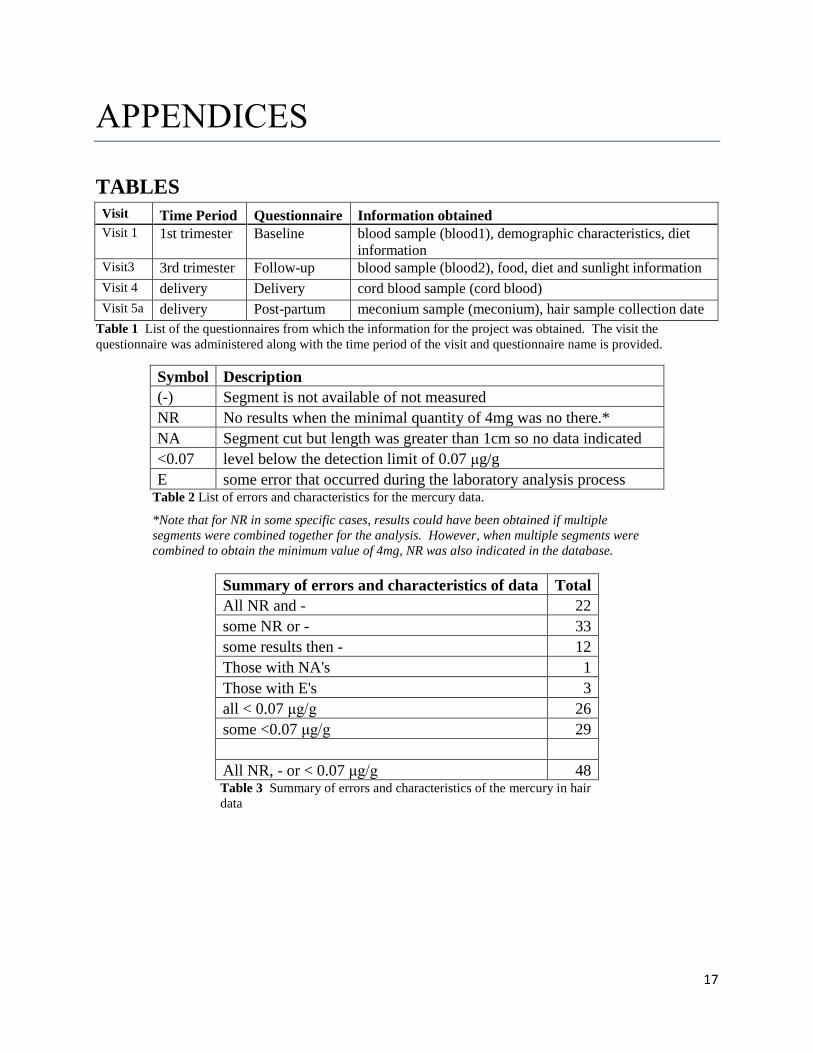
METHODS Brief description of errors and characteristics of hair sample dataset The hair samples provided were at most 12 cm in length. Each hair sample was cut into 1cm

segments giving at most 12 segments per participant and each of these segments was analyzed

for mercury. Table 6 gives a count of the number of samples per hair segment. A minimum of 4

mg of hair for each segment was required to analyze the total mercury content. The limit of

detection, LOD, was given at 0.07 µg Hg/g. If the detected mercury concentration was below

the LOD, “<0.07” was recorded. Errors and missing values resulted during analysis. The types

of errors and missing values can be found in table 1. Table 2 gives a brief summary of the

number of participants with different types and combinations of errors and characteristics.

Dating endpoints of hair segments In order to compare the mercury content in the hair with the corresponding blood sample, the

hair samples needed to be dated. Since each 1cm segment of the hair sample represents

approximately one month’s worth of hair growth, the dates of the endpoints of the hair segment

needed to be determined. This was done by finding the date of hair sample collection, hair_date,

from the hair collection dataset, hair_sample_col_nov, and working backwards. For example,

for a specified hair sample collection date was the first endpoint, point closest to the scalp, was

taken to be 3 weeks prior to that date. After that every endpoint, which was at 1cm intervals,

was taken to be approximately 1 month prior to that initial date. The approximation for 1 month

was taken as 30.42 days, 365 days / 12 months.

Pairing sample values with hair segment values In order to compare the mercury content in the blood, blood1, blood2, cord blood and meconium

samples, with that in the hair samples, the blood and meconium samples needed to be compared

to the correct 1cm hair segment. This entailed pairing up the blood and meconium sample

measurements with the corresponding hair segment by their dates. The dates for each of the

blood, cord blood and meconium samples were matched against the hair segment dates and given

a corresponding segment number representing the hair segment within which that particular

sample was collected. Once this was done that particular hair segment mercury content value

was compared to the corresponding sample value.

Postal codes Some exploratory analysis was done with the location of the individuals using the postal codes

provided. The first three characters of the postal code for each individual were provided. These

were looked at to approximate how many postal codes were for individuals in rural areas. Of the

350 individuals whose hair samples were analyzed, 20 had postal codes in the country side.

From the 20, only 2 were postal codes of individuals who were more than 20km away from one

of the cities given in table 3 thus suggesting that over 99% of the participants lived within or

close to metropolitan areas.

9

DATA PROCESSING

Working data set The MIREC study has many datasets stored under different databases, DACIMA and MIREC.

DACIMA had all the datasets that contain descriptive information from the questionnaires e.g.

eating habits; demographics information etc. while MIREC has datasets that contained measured

information from the questionnaires, e.g. blood sample measurements. The mercury hair sample

dataset came from a different source called PIERCE. As mentioned in the introduction there

were 1983 participants in MIREC. The mercury hair sample dataset consisted of a sample of

350 from the 1983 MIREC participants that provided hair samples, which was a total of 1282.

The information that was required to compare the mercury content in the hair segments to the

blood, cord blood and meconium samples were as follows: the collection dates of these samples,

i.e. collection dates for the blood samples, cord blood sample and meconium sample, the values

of this blood, cord blood and meconium samples. All these dates and values collected from

various datasets from the DACIMA and MIREC databases and then merged with the mercury

hair sample data set provided from PIERCE. This dataset was named “all”.

Baseline Information The various samples that are considered in this study, two blood samples, the first from Visit 1

and the second from Visit 3, the cord blood sample from Visit 4 and the meconium sample from

5a each had collection dates associated with them. These dates were also collected along with the

final hair sample collection date and the date of birth of the baby. This latter date was taken from

a dataset that was not in DACIMA or MIREC but from the dataset baby_dv_jan2016 that was

updated January 2016.

Socio-demographic information was collected at the beginning of the study in Visit 1 through the

baseline questionnaire. Information about the participant was obtained from here such as year of

birth, education level, marital status, ethnicity, living status, past pregnancies, high blood

pressure, chronic conditions and other some of which can be found in table 7. All the

information collected was for all the 1983 participants of the study. To obtain the relevant

information for the 350 participants whose hair samples were analyzed, the collected information

was merged by subject_id with the hair mercury dataset provided by PIERCE and those not part

of the mercury dataset provided by PIERCE were dropped from the final dataset.

ANALYSIS PLAN

The normal distribution and log normal distribution are referred to throughout this Analysis Plan,

Results and Conclusions. The normal or Gaussian distribution is a common probability

distribution and used often in the natural and social sciences. The probability density function

for the normal distribution for a random variable X is given by,

𝑓(𝑥) = 1

𝜎√2𝜋𝑒

−(𝑥−𝜇)2

2𝜎2 ,

10

where µ is the mean and 𝜎2 is the variance. A random variable X is said to have a log normal

distribution if the random 𝑌 = 𝑙𝑜𝑔𝑋 has a normal distribution.

The notation that will be used throughout is defined below. Summary tables of these variables

and their definitions can be found in table 5. Note that the lower the number of the hair segment

the closer the hair segment is to the scalp and thus pertains to time closer to the present while

larger numbered hair segments pertain to time points further in the past.

blood1 = blood sample taken at Visit 1.

blood2 = blood sample taken at Visit 3.

cord blood = cord blood sample taken at Visit 4.

meconium = meconium sample taken at Visit 5a.

𝐻𝑖𝑗 = mercury concentration for hair segment j for individual i paired with a given sample, i.e.

blood1, blood2, cord blood or meconium, where i=1, 2, …, 350 and 0 ≤ 𝑗 ≤ 12. 𝑛𝑖 = number of hair segments analyzed for individual i, where i = 1, 2, …., 350.

𝑎𝑣𝑔𝐻𝑖 =1

𝑛𝑖∑ 𝐻𝑖𝑗

𝑛𝑖𝑗=1 = average of all the hair segments analyzed for individual i, where i= 1, 2,

3….350 and 0 ≤ 𝑗 ≤ 12. 𝐻𝑘 = average mercury concentration for segment k, where k=1, 2, …. 12

Comparison of mercury in hair with blood samples

For each of the four comparisons, hair to blood1, blood2, cord blood and meconium, the process

below was completed; sample will refer to each one of blood1, blood2, cord blood or meconium.

The results of this process can be found in table 8 and in figures 6-33.

1. For the particular comparison, the date of collection of the sample was compared to all

the hair segment dates and its corresponding hair segment, 𝐻𝑖𝑗, recorded.

2. A plot of the mercury content in the corresponding hair segment 𝐻𝑖𝑗 vs the mercury

content in the sample was plotted.

3. In all cases the plot was very dense for smaller values and became sparser as the values

increased.

4. A log transformation was used and then a plot of log(𝐻𝑖𝑗) vs log(sample) was done.

5.

i. A linear regression was adjusted to measure/see if a linear relationship existed.

log(𝑠𝑎𝑚𝑝𝑙𝑒) = 𝛼 + 𝛽 log(𝐻𝑖𝑗) + 𝜀,

ii. with a 95% confidence.

iii. This was repeated for log(𝑠𝑎𝑚𝑝𝑙𝑒) ~log (𝑎𝑣𝑔𝐻𝑖).

iv. A residual plot in both cases was given. i.e. residuals of log(sample) vs log(𝐻𝑖𝑗) and

residuals of log(sample) vs log(𝑎𝑣𝑔𝐻𝑖).

v. A plot of log(sample) vs log(𝐻𝑖𝑗) and log(sample) vs log(𝑎𝑣𝑔𝐻𝑖) along with the

corresponding lines of best fit, 95% confidence limits and 95% prediction limits were

also made.

11

vi. Finally, 𝑅 2 and the Pearson correlation, ρ, were calculated in each case. Proc reg and

proc corr in SAS was used to perform the linear regression and Pearson correlation,

respectively.

6. Steps 1-5 were repeated using the average mercury concentration in the <12cm hair

sample for each participant, 𝑎𝑣𝑔𝐻𝑖.

Variability of mercury in hair samples

In order to determine the variability of mercury in hair samples, plots of the mercury content in

the hair segments were made. Results of the process below can be found in figures 2-5.

1. First a box plot of the mercury content by hair segment, 𝐻𝑖𝑗, was made.

2. Box plots of the log of the mercury content by hair segment, log(𝐻𝑖𝑗), were then done.

3. These box plots gave a distribution that appeared to be more normally distributed

implying that the mercury content in each of the segments is log normally distributed or

that the hair segments form a multivariate log normal distribution.

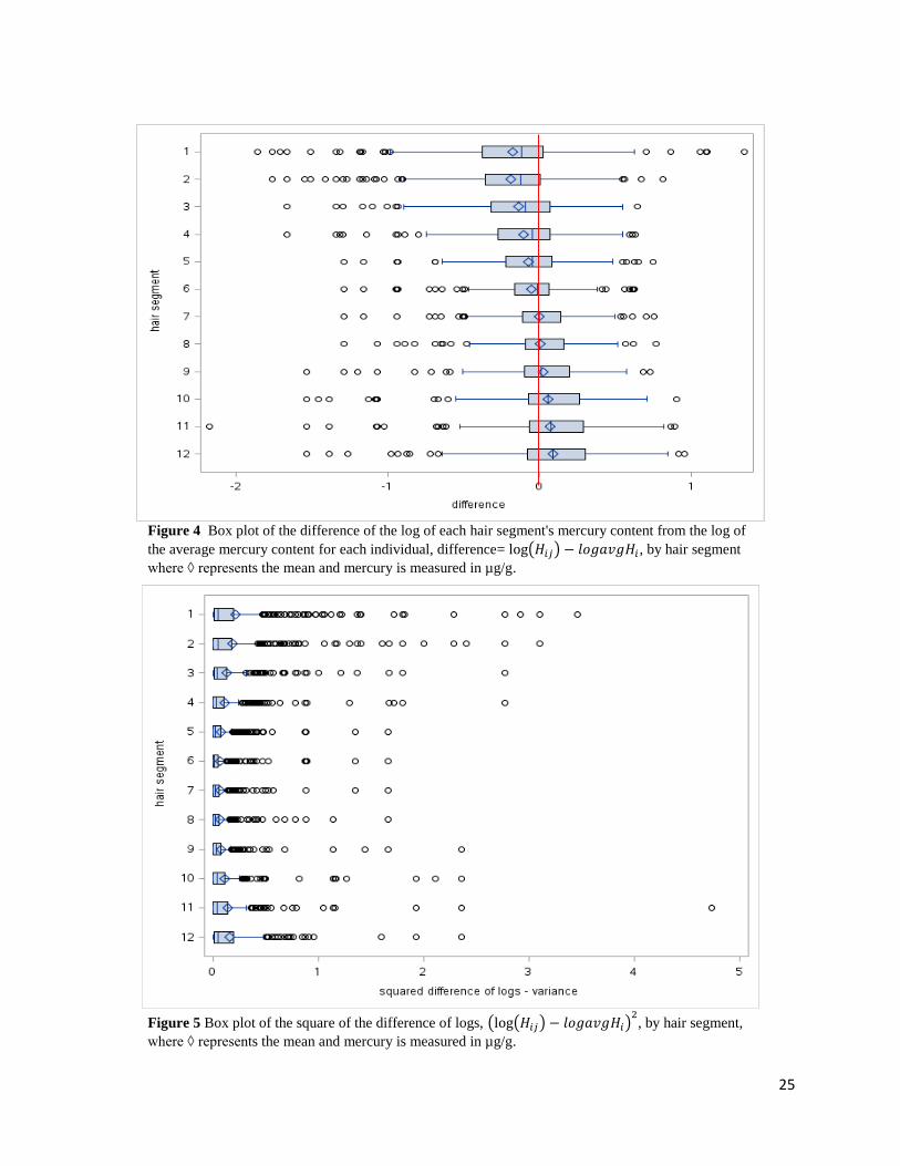
4. Box plots by hair segment for the difference between the log of the hair segment,

log(𝐻𝑖𝑗), from the log of the average of the hair segment, log(𝑎𝑣𝑔𝐻𝑖), i.e. log(𝐻𝑖𝑗) -

log(𝑎𝑣𝑔𝐻𝑖), for each individual were then done.

5. The means of this difference for each segment are near 0. However, it can be seen in

Figure 4 that the difference is greater in the first few hair segments, segments 1-4,

compared to the last few segments, segments 9-12. The few middle segments have a

smaller difference in means.

6. Box plots of the square of the difference of the logs, (log(𝐻𝑖𝑗) − log (𝑎𝑣𝑔𝐻𝑖))2, by hair

segments was also plotted.

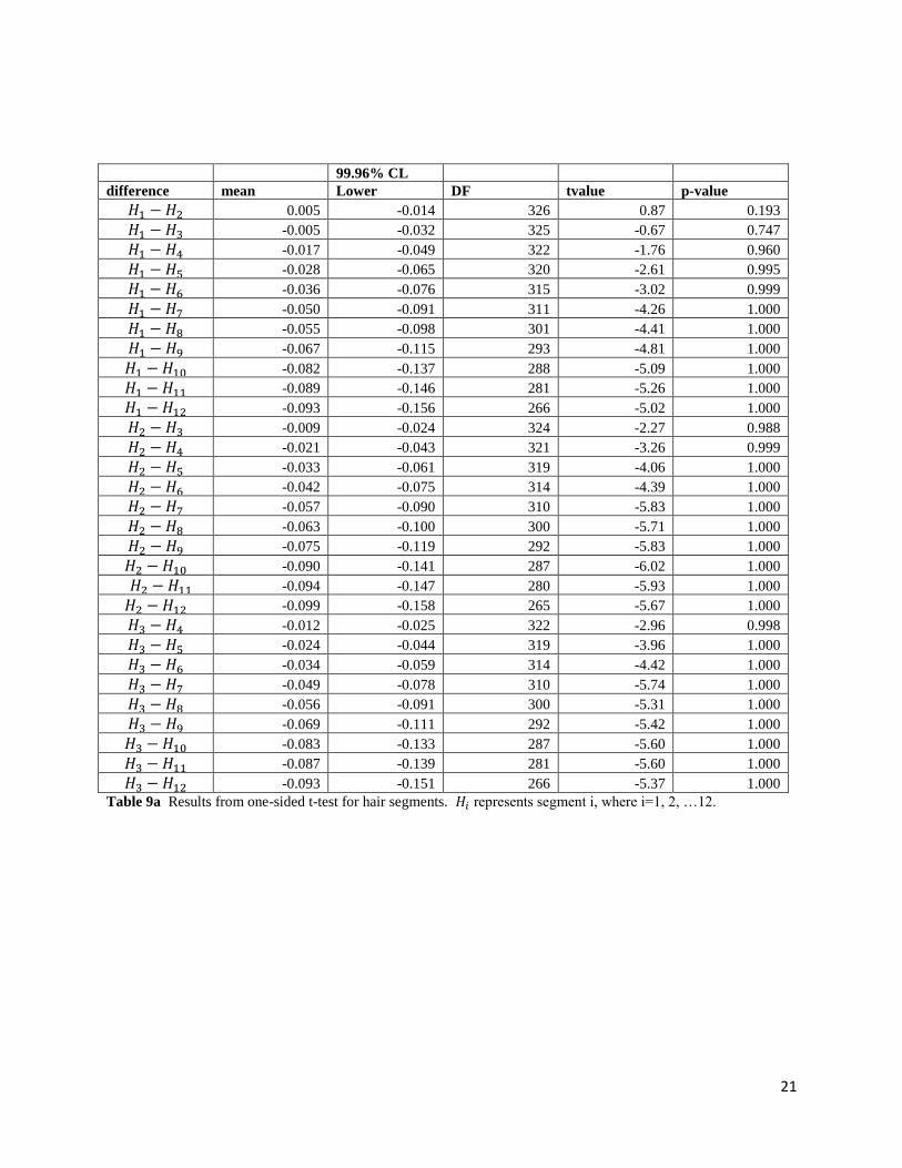
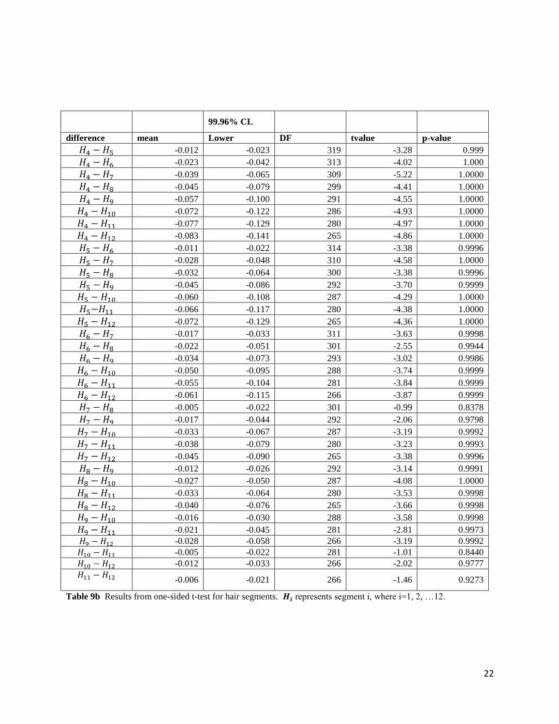
7. A series of one-sided t-tests with 𝛼 = 0.025/66 = 0.0004 where a Bonferroni correction

is used where 66 is the number of pairs that were compared, were done to show that the

mean mercury concentration between more distant hair segments was greater than for

adjacent and closer hair segments.

𝐻0: 𝐻𝑘 < 𝐻𝑙, 𝑘, 𝑙 = 1, 2, … , 12 𝑎𝑛𝑑 𝑘 < 𝑙.

12

RESULTS Subset description

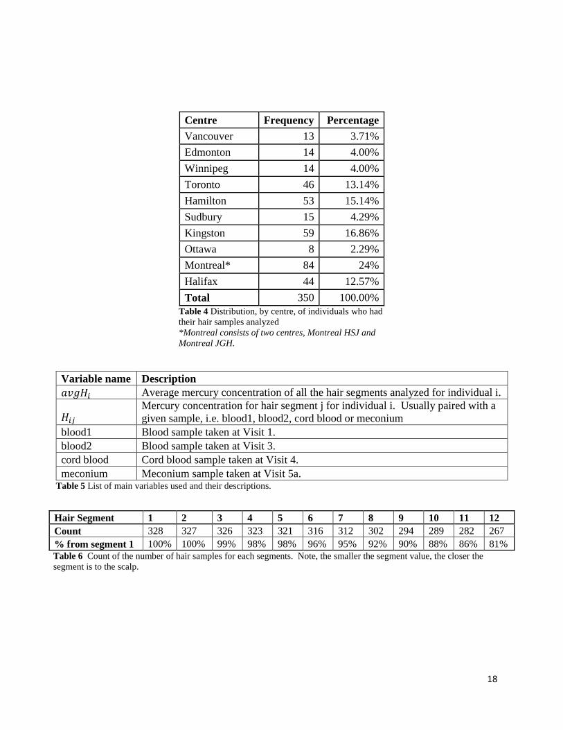
As noted in the introduction, 11 cities across Canada participated in the MIREC study for a total

of 1983 participants. The mean age of these participants was 32 years; 44% had no previous

viable pregnancy; 36% were overweight or obese based on pre-pregnancy BMI. From the 1983

participants, 1282 provided hair samples. Due to budgetary restrictions only 350 of these 1282

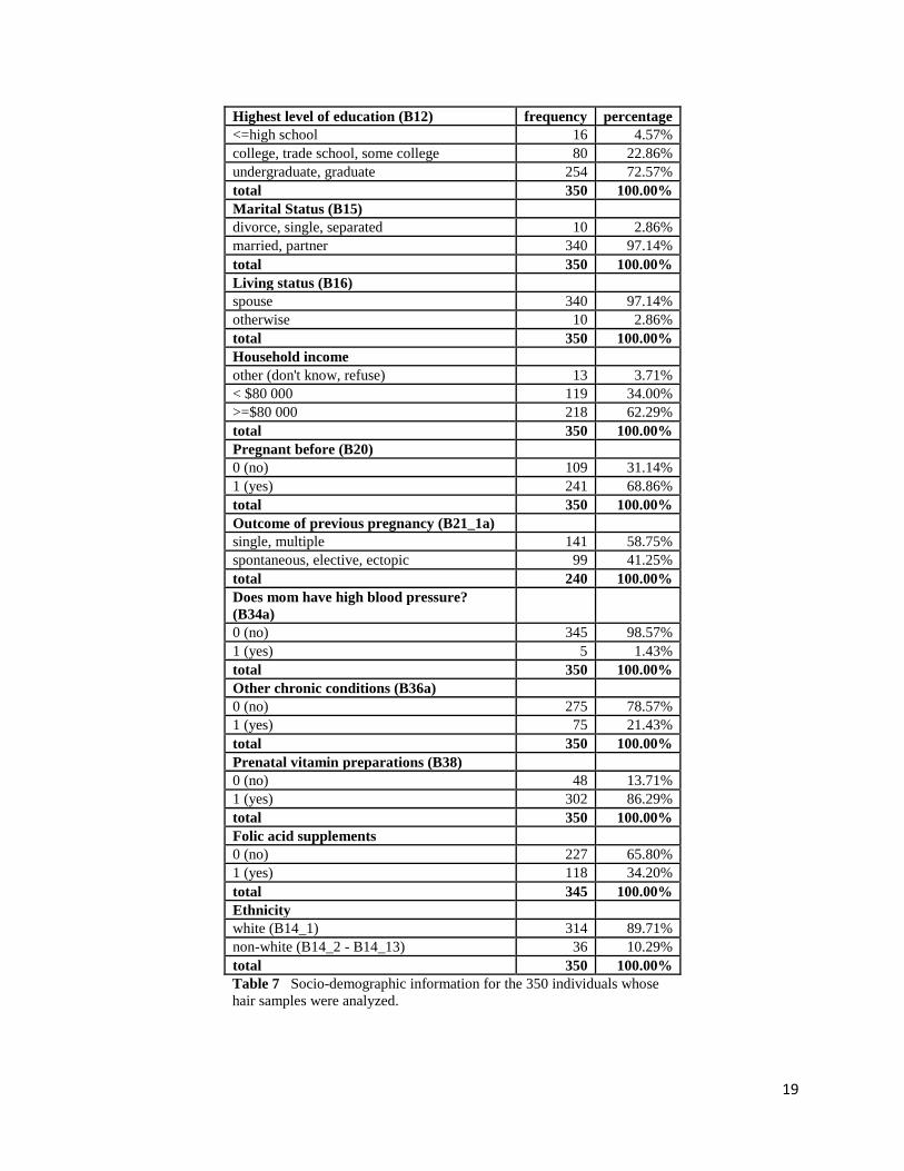
hair samples were analyzed. Table 3 and figure 1 give a distribution of the 350 individuals by

city. Table 4 gives an overview of the demographics of the 350 individuals whose hair samples

were analyzed. The results in table 4 correspond to what was observed from the MIREC

participants, the majority being higher educated and married or in a partner relationship. From

table 4 we can see that the majority of the individuals earn more than $80 000 (62%), have been

pregnant before (69%), do not have high blood pressure (98%), do not have chronic conditions

(78%) and are white (90%).

Comparison of mercury in hair with blood samples

Figures 6, 13, 20 and 27 provide plots of the mercury content in each of the samples, blood1,

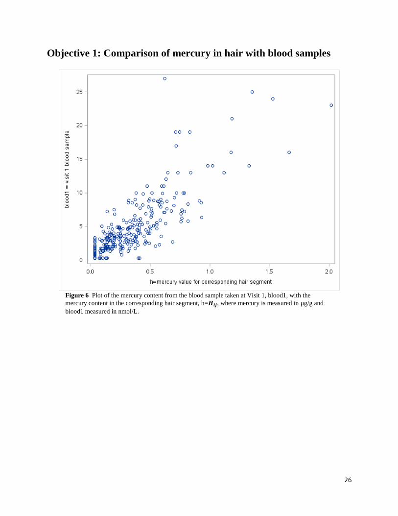
blood2, cord blood and meconium, vs 𝐻𝑖𝑗, respectively. Each of the plots is, for the most part,

denser for smaller values and become sparser for larger values and thus resembles the plot of

data that may log normally distributed. That is, if for example, blood1 follows a log normal

distribution then 𝑌1= log(blood1) will be normally distributed. Similarly for the 𝐻𝑖𝑗 values

paired to blood1. That is, 𝑌ℎ = log (𝐻𝑖𝑗) is also normally distributed. Once the log transformation

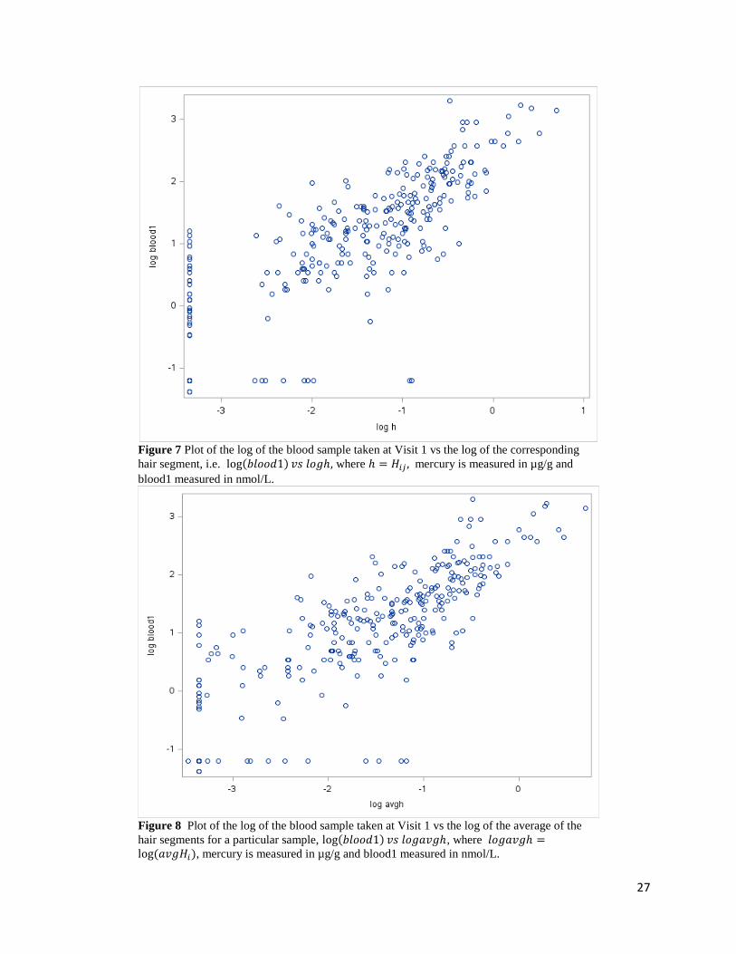
was performed on both the sample and 𝐻𝑖𝑗 a second series of plots were made. These may be

found in figures 7, 14, 21 and 28 for log(blood1), log(blood2), log(cord blood) and

log(meconium) vs log(𝐻𝑖𝑗), respectively. Each of the samples blood1, blood2 and cord blood

once transformed and plotted against log(𝐻𝑖𝑗) gave a much more evenly spread out plot, that is

denser in the middle than at the ends, thus resembling a normal distribution for log(sample) and

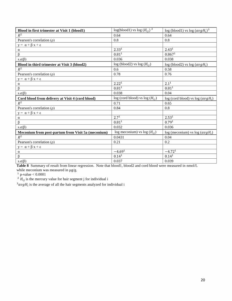
log(𝐻𝑖𝑗). These plots also suggest a linear relationship between log(sample) vs log(𝐻𝑖𝑗). Details

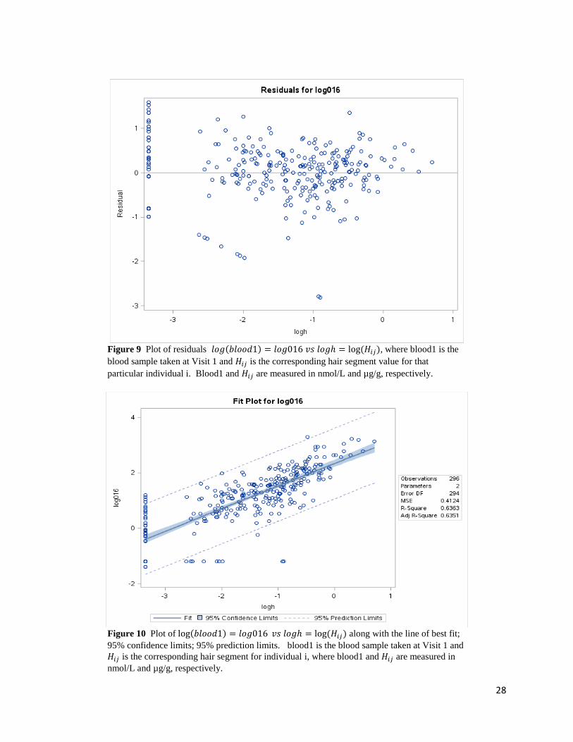
of this linear relationship can be found in table 8. Notice the linear regression models for

log(sample) vs log(𝐻𝑖𝑗), where sample is blood1, blood2 and cord blood, the 𝑅2 values range

between 0.6-0.7 and Pearson’s correlation is around 0.8 suggesting a linear relationship.

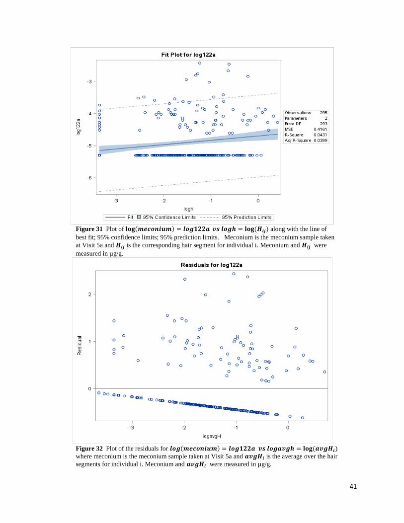
However, for log(meconium) vs log(𝐻𝑖𝑗) these two values are much lower, 𝑅2 = 0.043 and a

Pearson correlation of 0.21, suggesting that there is a weak or no linear relationship between the

two. This can be seen in the transformed meconium plot given in figure 28, while more spread

out, it is not clear what the trend is. There are many values for meconium that are 0 or below the

level of detection.

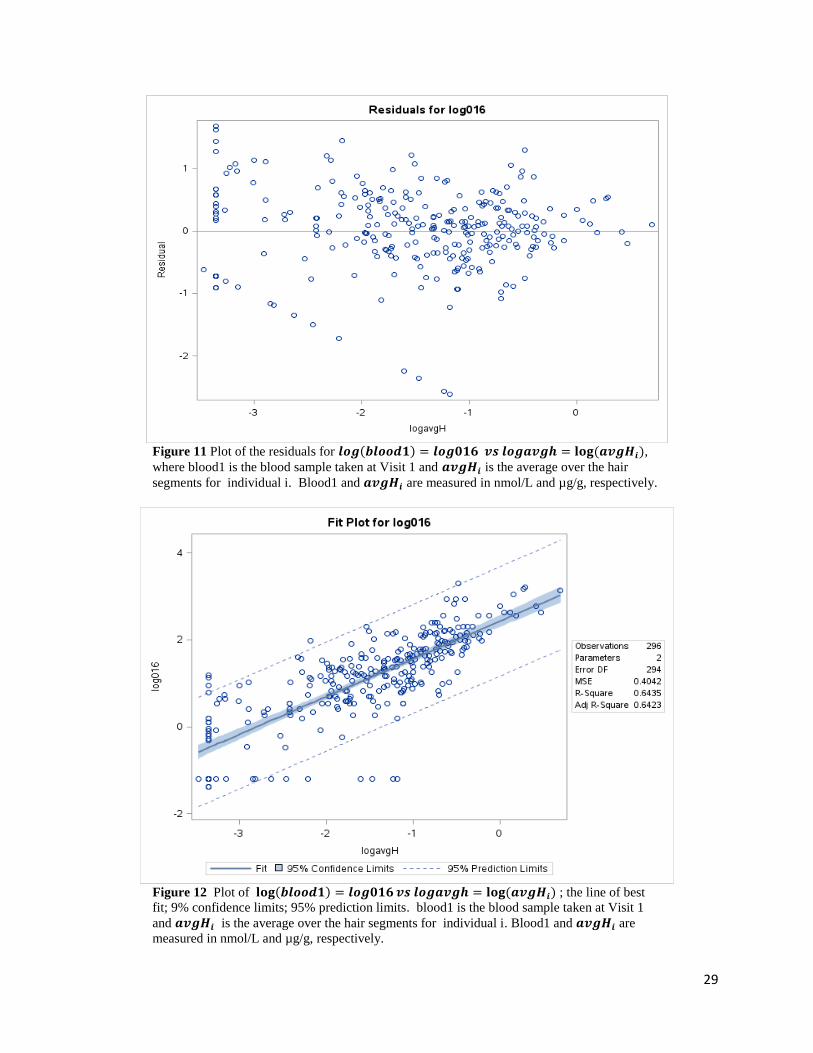
As mentioned in the Methods section, the average of the mercury content across all the hair

segments for each participant was also considered. The log transformation and corresponding

plots were made for log(blood1), log(blood2), log(cord blood) and log(meconium) vs

log(𝑎𝑣𝑔𝐻𝑖). These may be found in figures 8, 15, 22 and 29, respectively. These plots look

very similar to those in figures 7, 14, 21 and 28, respectively and may suggest that considering

13

the average mercury content over a period of months or over a longer hair sample may be

sufficient rather than trying to pair the sample to a hair segment by date. Even when paired, we

are not sure the pairing is accurate due to the different growth rates for hair. This can also be

seen when comparing the residual plots. For example, comparing figures 9 and 11, the residuals

of log(blood1) vs log(𝐻𝑖𝑗) and log(𝑎𝑣𝑔𝐻𝑖), respectively. Both plots look very similar. The

plots in figures 10 and 12 of log(blood1) vs log(𝐻𝑖𝑗) and log(𝑎𝑣𝑔𝐻𝑖), respectively, and their

respective line of best fit are also very similar. Table 8 provides the coefficients for the lines of

best fit for each and the coefficients are very close in value. The same pattern for the residual

plots, line of best fit plots and coefficient values for the other samples, blood2, cord blood and

meconium can be found when comparing figures 16 and 18; 23 and 25; 30 and 32, respectively.

Table 8 presents all the results for the linear models log(sample) vs log(𝐻𝑖𝑗) and log(sample) vs

log(𝑎𝑣𝑔𝐻𝑖), where sample takes on values blood1, blood2, cord blood or meconium. The

models involving meconium have very small 𝑅2 and Pearson correlation values suggesting that a

linear relationship for the transformed meconium values is not the best.

Variability of mercury in hair samples

In figure 2 a simple box plot of the mercury content in each segment of the hair sample is plotted

by hair segment for all participants. It is quite clear that the values are skewed towards the left.

A lot transformation is performed on the mercury values in each hair segment then plotted by

hair segment in figure 3. The distributions for each hair segment are more normally distributed.

In figure 4 a plot of the difference in logs, log(𝐻𝑖𝑗) - log(𝑎𝑣𝑔𝐻𝑖), is made by segment. Again,

the distribution for each segment seems normally distributed. In this case we notice that the hair

segments at the ends of the hair sample have the widest range of values. The distribution for all

hair segments seem to have means near 0. Finally, in figure 5 a plot of the square of the

difference of logs by segments is made, i.e. (log(𝐻𝑖𝑗) − log (𝑎𝑣𝑔𝐻𝑖))2. Again, the variability is

greatest at the end segments of the hair sample and decreases as the mid segments are

approached. In this situation the range of values is largest in the first few hair segments,

decreases towards the mid segments then increases again towards the other end however not to

the extent as for the first few segments. This was verified through paired t tests for the mean

mercury concentration by hair segment. The results of these one-sided t tests can be found in

tables 9a and 9b. All of the differences of mean mercury concentration by hair segment, 𝐻𝑖 − 𝐻𝑗

where 𝑖 ≠ 𝑗 and i, j=1, 2, …., 12 and 𝑖 < 𝑗, are not significantly greater than 0.

14

CONCLUSIONS Comparison of mercury in hair with blood samples

The mercury concentration in hair samples with that of collected samples, blood1, blood2, cord

blood and meconium, was done first through a series of plots to see if there is a relationship

between the hair sample concentration and that of the collected sample. In all cases the results

are log normally distributed. i.e. blood1, blood2, cord blood, meconium, 𝐻𝑖𝑗 and 𝑎𝑣𝑔𝐻𝑖 all seem

to be log normally distributed. After transforming the variables the relationship for three out of

the four variables in particular, blood1, blood2 and cord blood, seems to be linear with respect to

log (𝐻𝑖𝑗) and log (𝑎𝑣𝑔𝐻𝑖). It was found that using a hair segment 𝐻𝑖𝑗 paired to the sample gave a

result very close to that of just taking the average of all the hair segments 𝑎𝑣𝑔𝐻𝑖.

Variability of mercury in hair samples

The variability of the mercury concentration in the hair samples was seen to follow a log normal

distribution by segment. It was also noted that the range of the mercury values in the hair

samples was greater at one end of the hair samples and lower closer to the scalp. The variability

of the mean mercury concentration by segment was greater the farther apart the segments were.

That is, segment 1 and segment 12 have mean values that a farther apart than segments 1 and 2,

for example. This is shown in Figure 4 and verified through the one-sided t tests in tables 9a and

9b.

15

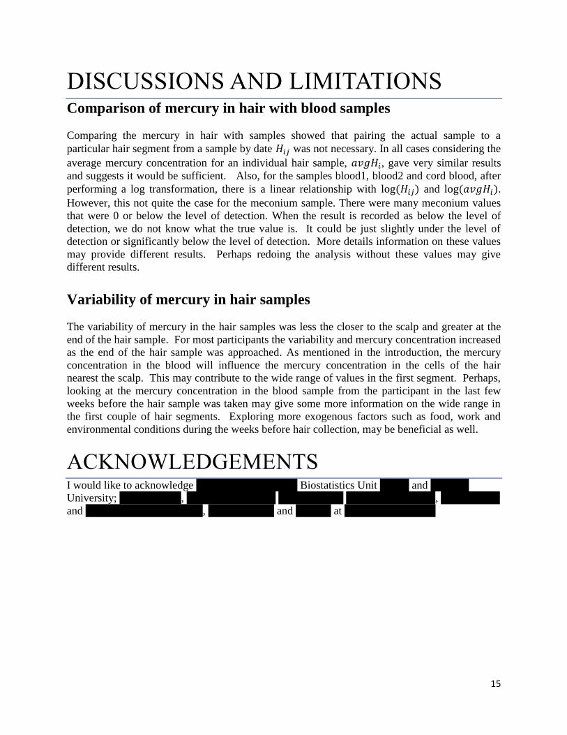
DISCUSSIONS AND LIMITATIONS Comparison of mercury in hair with blood samples

Comparing the mercury in hair with samples showed that pairing the actual sample to a

particular hair segment from a sample by date 𝐻𝑖𝑗 was not necessary. In all cases considering the

average mercury concentration for an individual hair sample, 𝑎𝑣𝑔𝐻𝑖, gave very similar results

and suggests it would be sufficient. Also, for the samples blood1, blood2 and cord blood, after

performing a log transformation, there is a linear relationship with log (𝐻𝑖𝑗) and log (𝑎𝑣𝑔𝐻𝑖).

However, this not quite the case for the meconium sample. There were many meconium values

that were 0 or below the level of detection. When the result is recorded as below the level of

detection, we do not know what the true value is. It could be just slightly under the level of

detection or significantly below the level of detection. More details information on these values

may provide different results. Perhaps redoing the analysis without these values may give

different results.

Variability of mercury in hair samples

The variability of mercury in the hair samples was less the closer to the scalp and greater at the

end of the hair sample. For most participants the variability and mercury concentration increased

as the end of the hair sample was approached. As mentioned in the introduction, the mercury

concentration in the blood will influence the mercury concentration in the cells of the hair

nearest the scalp. This may contribute to the wide range of values in the first segment. Perhaps,

looking at the mercury concentration in the blood sample from the participant in the last few

weeks before the hair sample was taken may give some more information on the wide range in

the first couple of hair segments. Exploring more exogenous factors such as food, work and

environmental conditions during the weeks before hair collection, may be beneficial as well.

ACKNOWLEDGEMENTS I would like to acknowledge Health Canada and the Biostatistics Unit (BSU) and Carleton

University; Tye Arbuckle, Monique D’Amour, Mandy Fisher, Mary Alice Hefford, Mike Walker

and Gabriela Williams at BSU, Health Canada and Dr. Rao at Carleton University.

16

REFERENCES 1. Mercury Contamination in Fish, Url: http://www.nrdc.org/health/effects/mercury/sources.asp

2. What you need to know about the different forms of Mercury, the next generation of mercury

testing, and how to detox safely, Url:

http://articles.mercola.com/sites/articles/archive/2013/01/06/dr-shade-on-mercury-

exposure.aspx

3. Mercury and Human Health, Url: http://www.hc-sc.gc.ca/hl-vs/iyh-vsv/environ/merc-

eng.php

4. General information about mercury and mercury exposure, Url:

http://www.medicinenet.com/mercury_poisoning/page2.htm

5. Sources of Heavy Metal Poisoning, Url: http://www.evenbetterhealth.com/heavy-metal-

poisoning-sources.php

6. Environmental toxicants and fetal development, Url:

https://en.wikipedia.org/wiki/Environmental_toxicants_and_fetal_development

7. Heavy Metal Detox & Glutathione Connection, Url:

http://www.naturalguidetohealth.com/heavymetaldetoxandglutathione.html

8. Sources of Mercury https://www.ec.gc.ca/mercure-

mercury/default.asp?lang=En&n=EB9F5205-1

9. D. Bernhard, A. Rossman, G. Wick, Critical Review Metals in Cigarette Smoke, IUBMB

Life, Vol 57, Iss. 12, pp. 805-809, December 2005.

10. Tye E. Arbuckle et al., Cohort Profile: The Maternal-Infant Research on Environmental

Chemicals Research Platform, Paediatric and Perinatal Epidemiology, 2013, Vol. 27, pp.

415-425.

11. MIREC Data Users, URL:

http://www.gcpedia.gc.ca/wiki/User:Branka.Jovic/sandbox/MIREC_Data_Users

12. Mercury in Human Hair Due to Environment and Diet: A Review, D. Airey, Environmental

Health Perspectives, Vol. 52, pp. 303-316, 1983.

13. Background information on MIREC mercury in hair project, this was provided to us in

January 2016.

14. Nuttal, Kern L., Review: Interpreting Hair Mercury levels in Individual Patients, Annals of

Clinical & Laboratory Science, Vol. 36, No. 3, 2006, pp. 248-261.

17

APPENDICES

TABLES

Visit Time Period Questionnaire Information obtained

Visit 1 1st trimester Baseline blood sample (blood1), demographic characteristics, diet

information Visit3 3rd trimester Follow-up blood sample (blood2), food, diet and sunlight information

Visit 4 delivery Delivery cord blood sample (cord blood)

Visit 5a delivery Post-partum meconium sample (meconium), hair sample collection date

Table 1 List of the questionnaires from which the information for the project was obtained. The visit the

questionnaire was administered along with the time period of the visit and questionnaire name is provided.

Symbol Description

(-) Segment is not available of not measured

NR No results when the minimal quantity of 4mg was no there.*

NA Segment cut but length was greater than 1cm so no data indicated

<0.07 level below the detection limit of 0.07 μg/g

E some error that occurred during the laboratory analysis process Table 2 List of errors and characteristics for the mercury data.

*Note that for NR in some specific cases, results could have been obtained if multiple

segments were combined together for the analysis. However, when multiple segments were

combined to obtain the minimum value of 4mg, NR was also indicated in the database.

Summary of errors and characteristics of data Total

All NR and - 22

some NR or - 33

some results then - 12

Those with NA's 1

Those with E's 3

all < 0.07 μg/g 26

some <0.07 μg/g 29

All NR, - or < 0.07 μg/g 48 Table 3 Summary of errors and characteristics of the mercury in hair

data

18

Centre Frequency Percentage

Vancouver 13 3.71%

Edmonton 14 4.00%

Winnipeg 14 4.00%

Toronto 46 13.14%

Hamilton 53 15.14%

Sudbury 15 4.29%

Kingston 59 16.86%

Ottawa 8 2.29%

Montreal* 84 24%

Halifax 44 12.57%

Total 350 100.00%

Table 4 Distribution, by centre, of individuals who had

their hair samples analyzed

*Montreal consists of two centres, Montreal HSJ and

Montreal JGH.

Variable name Description

𝑎𝑣𝑔𝐻𝑖 Average mercury concentration of all the hair segments analyzed for individual i.

𝐻𝑖𝑗 Mercury concentration for hair segment j for individual i. Usually paired with a

given sample, i.e. blood1, blood2, cord blood or meconium

blood1 Blood sample taken at Visit 1.

blood2 Blood sample taken at Visit 3.

cord blood Cord blood sample taken at Visit 4.

meconium Meconium sample taken at Visit 5a. Table 5 List of main variables used and their descriptions.

Hair Segment 1 2 3 4 5 6 7 8 9 10 11 12

Count 328 327 326 323 321 316 312 302 294 289 282 267

% from segment 1 100% 100% 99% 98% 98% 96% 95% 92% 90% 88% 86% 81%

Table 6 Count of the number of hair samples for each segments. Note, the smaller the segment value, the closer the

segment is to the scalp.

19

Highest level of education (B12) frequency percentage

<=high school 16 4.57%

college, trade school, some college 80 22.86%

undergraduate, graduate 254 72.57%

total 350 100.00%

Marital Status (B15)

divorce, single, separated 10 2.86%

married, partner 340 97.14%

total 350 100.00%

Living status (B16)

spouse 340 97.14%

otherwise 10 2.86%

total 350 100.00%

Household income

other (don't know, refuse) 13 3.71%

< $80 000 119 34.00%

>=$80 000 218 62.29%

total 350 100.00%

Pregnant before (B20)

0 (no) 109 31.14%

1 (yes) 241 68.86%

total 350 100.00%

Outcome of previous pregnancy (B21_1a)

single, multiple 141 58.75%

spontaneous, elective, ectopic 99 41.25%

total 240 100.00%

Does mom have high blood pressure?

(B34a)

0 (no) 345 98.57%

1 (yes) 5 1.43%

total 350 100.00%

Other chronic conditions (B36a)

0 (no) 275 78.57%

1 (yes) 75 21.43%

total 350 100.00%

Prenatal vitamin preparations (B38)

0 (no) 48 13.71%

1 (yes) 302 86.29%

total 350 100.00%

Folic acid supplements

0 (no) 227 65.80%

1 (yes) 118 34.20%

total 345 100.00%

Ethnicity

white (B14_1) 314 89.71%

non-white (B14_2 - B14_13) 36 10.29%

total 350 100.00%

Table 7 Socio-demographic information for the 350 individuals whose

hair samples were analyzed.

20

Blood in first trimester at Visit 1 (blood1) log(blood1) vs log (𝐻𝑖𝑗) 2 log (blood1) vs log (𝑎𝑣𝑔𝐻𝑖)3

𝑅2 0.64 0.64

Pearson's correlation (ρ) 0.8 0.8

y = α + β x + ε

α 2.331 2.431

β 0.811 0.8671

s.e(β) 0.036 0.038

Blood in third trimester at Visit 3 (blood2) log (blood2) vs log (𝐻𝑖𝑗) log (blood2) vs log (𝑎𝑣𝑔𝐻𝑖)

𝑅2 0.6 0.58

Pearson's correlation (ρ) 0.78 0.76

y = α + β x + ε

α 2.221 2.11

β 0.811 0.811

s.e(β) 0.038 0.04

Cord blood from delivery at Visit 4 (cord blood) log (cord blood) vs log (𝐻𝑖𝑗) log (cord blood) vs log (𝑎𝑣𝑔𝐻𝑖)

𝑅2 0.71 0.65

Pearson's correlation (ρ) 0.84 0.8

y = α + β x + ε

α 2.71 2.531

β 0.811 0.791

s.e(β) 0.032 0.036

Meconium from post-partum from Visit 5a (meconium) log meconium) vs log (𝐻𝑖𝑗) log (meconium) vs log (𝑎𝑣𝑔𝐻𝑖)

𝑅2 0.0431 0.04

Pearson's correlation (ρ) 0.21 0.2

y = α + β x + ε

α −4.691 −4.721

β 0.141 0.141

s.e(β) 0.037 0.039

Table 8 Summary of result from linear regression. Note that blood1, blood2 and cord blood were measured in nmol/L

while meconium was measured in µg/g.

1 p-value < 0.0001

2 𝐻𝑖𝑗 is the mercury value for hair segment j for individual i

𝑎𝑣𝑔𝐻𝑖 3 is the average of all the hair segments analyzed for individual i

21

99.96% CL

difference mean Lower DF tvalue p-value

𝐻1 − 𝐻2 0.005 -0.014 326 0.87 0.193

𝐻1 − 𝐻3 -0.005 -0.032 325 -0.67 0.747

𝐻1 − 𝐻4 -0.017 -0.049 322 -1.76 0.960

𝐻1 − 𝐻5 -0.028 -0.065 320 -2.61 0.995

𝐻1 − 𝐻6 -0.036 -0.076 315 -3.02 0.999

𝐻1 − 𝐻7 -0.050 -0.091 311 -4.26 1.000

𝐻1 − 𝐻8 -0.055 -0.098 301 -4.41 1.000

𝐻1 − 𝐻9 -0.067 -0.115 293 -4.81 1.000

𝐻1 − 𝐻10 -0.082 -0.137 288 -5.09 1.000

𝐻1 − 𝐻11 -0.089 -0.146 281 -5.26 1.000

𝐻1 − 𝐻12 -0.093 -0.156 266 -5.02 1.000

𝐻2 − 𝐻3 -0.009 -0.024 324 -2.27 0.988

𝐻2 − 𝐻4 -0.021 -0.043 321 -3.26 0.999

𝐻2 − 𝐻5 -0.033 -0.061 319 -4.06 1.000

𝐻2 − 𝐻6 -0.042 -0.075 314 -4.39 1.000

𝐻2 − 𝐻7 -0.057 -0.090 310 -5.83 1.000

𝐻2 − 𝐻8 -0.063 -0.100 300 -5.71 1.000

𝐻2 − 𝐻9 -0.075 -0.119 292 -5.83 1.000

𝐻2 − 𝐻10 -0.090 -0.141 287 -6.02 1.000

𝐻2 − 𝐻11 -0.094 -0.147 280 -5.93 1.000

𝐻2 − 𝐻12 -0.099 -0.158 265 -5.67 1.000

𝐻3 − 𝐻4 -0.012 -0.025 322 -2.96 0.998

𝐻3 − 𝐻5 -0.024 -0.044 319 -3.96 1.000

𝐻3 − 𝐻6 -0.034 -0.059 314 -4.42 1.000

𝐻3 − 𝐻7 -0.049 -0.078 310 -5.74 1.000

𝐻3 − 𝐻8 -0.056 -0.091 300 -5.31 1.000

𝐻3 − 𝐻9 -0.069 -0.111 292 -5.42 1.000

𝐻3 − 𝐻10 -0.083 -0.133 287 -5.60 1.000

𝐻3 − 𝐻11 -0.087 -0.139 281 -5.60 1.000

𝐻3 − 𝐻12 -0.093 -0.151 266 -5.37 1.000

Table 9a Results from one-sided t-test for hair segments. 𝐻𝑖 represents segment i, where i=1, 2, …12.

22

99.96% CL

difference mean Lower DF tvalue p-value

𝐻4 − 𝐻5 -0.012 -0.023 319 -3.28 0.999

𝐻4 − 𝐻6 -0.023 -0.042 313 -4.02 1.000

𝐻4 − 𝐻7 -0.039 -0.065 309 -5.22 1.0000

𝐻4 − 𝐻8 -0.045 -0.079 299 -4.41 1.0000

𝐻4 − 𝐻9 -0.057 -0.100 291 -4.55 1.0000

𝐻4 − 𝐻10 -0.072 -0.122 286 -4.93 1.0000

𝐻4 − 𝐻11 -0.077 -0.129 280 -4.97 1.0000

𝐻4 − 𝐻12 -0.083 -0.141 265 -4.86 1.0000

𝐻5 − 𝐻6 -0.011 -0.022 314 -3.38 0.9996

𝐻5 − 𝐻7 -0.028 -0.048 310 -4.58 1.0000

𝐻5 − 𝐻8 -0.032 -0.064 300 -3.38 0.9996

𝐻5 − 𝐻9 -0.045 -0.086 292 -3.70 0.9999

𝐻5 − 𝐻10 -0.060 -0.108 287 -4.29 1.0000

𝐻5−𝐻11 -0.066 -0.117 280 -4.38 1.0000

𝐻5 − 𝐻12 -0.072 -0.129 265 -4.36 1.0000

𝐻6 − 𝐻7 -0.017 -0.033 311 -3.63 0.9998

𝐻6 − 𝐻8 -0.022 -0.051 301 -2.55 0.9944

𝐻6 − 𝐻9 -0.034 -0.073 293 -3.02 0.9986

𝐻6 − 𝐻10 -0.050 -0.095 288 -3.74 0.9999

𝐻6 − 𝐻11 -0.055 -0.104 281 -3.84 0.9999

𝐻6 − 𝐻12 -0.061 -0.115 266 -3.87 0.9999

𝐻7 − 𝐻8 -0.005 -0.022 301 -0.99 0.8378

𝐻7 − 𝐻9 -0.017 -0.044 292 -2.06 0.9798

𝐻7 − 𝐻10 -0.033 -0.067 287 -3.19 0.9992

𝐻7 − 𝐻11 -0.038 -0.079 280 -3.23 0.9993

𝐻7 − 𝐻12 -0.045 -0.090 265 -3.38 0.9996

𝐻8 − 𝐻9 -0.012 -0.026 292 -3.14 0.9991

𝐻8 − 𝐻10 -0.027 -0.050 287 -4.08 1.0000

𝐻8 − 𝐻11 -0.033 -0.064 280 -3.53 0.9998

𝐻8 − 𝐻12 -0.040 -0.076 265 -3.66 0.9998

𝐻9 − 𝐻10 -0.016 -0.030 288 -3.58 0.9998

𝐻9 − 𝐻11 -0.021 -0.045 281 -2.81 0.9973

𝐻9 − 𝐻12 -0.028 -0.058 266 -3.19 0.9992

𝐻10 − 𝐻11 -0.005 -0.022 281 -1.01 0.8440

𝐻10 − 𝐻12 -0.012 -0.033 266 -2.02 0.9777

𝐻11 − 𝐻12

-0.006 -0.021 266 -1.46 0.9273

Table 9b Results from one-sided t-test for hair segments. 𝑯𝒊 represents segment i, where i=1, 2, …12.

23

FIGURES

Figure 1 Distribution of the 350 participants' analyzed hair samples by centre

13 14 14

4653

15

59

8

80

4

44

0

10

20

30

40

50

60

70

80

90

Centre

Table 9 Results from paired t test for hair segments. 𝐻𝑖 represents segment i, where i=1, 2, …12.

24

Objective 2: Variability of mercury in hair samples

Figure 2 Box plot of mercury concentration in hair samples by segment where ◊ represents the mean

and mercury is measured in µg/g.

Figure 3 Box plot of log of mercury concentration, logHg, in hair samples by hair segment where ◊

represents the mean and mercury is measured in µg/g.

25

Figure 4 Box plot of the difference of the log of each hair segment's mercury content from the log of

the average mercury content for each individual, difference= log(𝐻𝑖𝑗) − 𝑙𝑜𝑔𝑎𝑣𝑔𝐻𝑖 , by hair segment

where ◊ represents the mean and mercury is measured in µg/g.

Figure 5 Box plot of the square of the difference of logs, (log(𝐻𝑖𝑗) − 𝑙𝑜𝑔𝑎𝑣𝑔𝐻𝑖)

2, by hair segment,

where ◊ represents the mean and mercury is measured in µg/g.

26

Objective 1: Comparison of mercury in hair with blood samples

Figure 6 Plot of the mercury content from the blood sample taken at Visit 1, blood1, with the

mercury content in the corresponding hair segment, h=𝑯𝒊𝒋, where mercury is measured in µg/g and

blood1 measured in nmol/L.

27

Figure 7 Plot of the log of the blood sample taken at Visit 1 vs the log of the corresponding

hair segment, i.e. log(𝑏𝑙𝑜𝑜𝑑1) 𝑣𝑠 𝑙𝑜𝑔ℎ, where ℎ = 𝐻𝑖𝑗 , mercury is measured in µg/g and

blood1 measured in nmol/L.

Figure 8 Plot of the log of the blood sample taken at Visit 1 vs the log of the average of the

hair segments for a particular sample, log(𝑏𝑙𝑜𝑜𝑑1) 𝑣𝑠 𝑙𝑜𝑔𝑎𝑣𝑔ℎ, where 𝑙𝑜𝑔𝑎𝑣𝑔ℎ =log (𝑎𝑣𝑔𝐻𝑖), mercury is measured in µg/g and blood1 measured in nmol/L.

28

Figure 9 Plot of residuals 𝑙𝑜𝑔(𝑏𝑙𝑜𝑜𝑑1) = 𝑙𝑜𝑔016 𝑣𝑠 𝑙𝑜𝑔ℎ = log (𝐻𝑖𝑗), where blood1 is the

blood sample taken at Visit 1 and 𝐻𝑖𝑗 is the corresponding hair segment value for that

particular individual i. Blood1 and 𝐻𝑖𝑗 are measured in nmol/L and µg/g, respectively.

Figure 10 Plot of log(𝑏𝑙𝑜𝑜𝑑1) = 𝑙𝑜𝑔016 𝑣𝑠 𝑙𝑜𝑔ℎ = log (𝐻𝑖𝑗) along with the line of best fit;

95% confidence limits; 95% prediction limits. blood1 is the blood sample taken at Visit 1 and

𝐻𝑖𝑗 is the corresponding hair segment for individual i, where blood1 and 𝐻𝑖𝑗 are measured in

nmol/L and µg/g, respectively.

29

Figure 11 Plot of the residuals for 𝒍𝒐𝒈(𝒃𝒍𝒐𝒐𝒅𝟏) = 𝒍𝒐𝒈𝟎𝟏𝟔 𝒗𝒔 𝒍𝒐𝒈𝒂𝒗𝒈𝒉 = 𝐥𝐨𝐠 (𝒂𝒗𝒈𝑯𝒊),

where blood1 is the blood sample taken at Visit 1 and 𝒂𝒗𝒈𝑯𝒊 is the average over the hair

segments for individual i. Blood1 and 𝒂𝒗𝒈𝑯𝒊 are measured in nmol/L and µg/g, respectively.

Figure 12 Plot of 𝐥𝐨𝐠(𝒃𝒍𝒐𝒐𝒅𝟏) = 𝒍𝒐𝒈𝟎𝟏𝟔 𝒗𝒔 𝒍𝒐𝒈𝒂𝒗𝒈𝒉 = 𝐥𝐨𝐠 (𝒂𝒗𝒈𝑯𝒊) ; the line of best

fit; 9% confidence limits; 95% prediction limits. blood1 is the blood sample taken at Visit 1

and 𝒂𝒗𝒈𝑯𝒊 is the average over the hair segments for individual i. Blood1 and 𝒂𝒗𝒈𝑯𝒊 are

measured in nmol/L and µg/g, respectively.

30

Figure 13 Plot of the mercury content from the blood sample taken at Visit 3, blood2,

with the mercury content in the corresponding hair segment, h=𝑯𝒊𝒋 where blood2 and

𝑯𝒊𝒋are measured in nmol/L and µg/g, respectively.

Figure 14 Plot of the log of the blood sample taken at Visit 3 vs the log of the

corresponding hair segment, i.e. 𝐥𝐨𝐠(𝒃𝒍𝒐𝒐𝒅𝟐) 𝒗𝒔 𝒍𝒐𝒈𝒉, where 𝒉 = 𝑯𝒊𝒋, blood2 and

𝑯𝒊𝒋are measured in nmol/L and µg/g, respectively.

31

Figure 15 Plot of the log of the blood sample taken at Visit 2 vs the log of the average of the hair segments for a

particular sample, 𝐥𝐨𝐠(𝒃𝒍𝒐𝒐𝒅𝟐) 𝒗𝒔 𝒍𝒐𝒈𝒂𝒗𝒈𝒉, where 𝒍𝒐𝒈𝒂𝒗𝒈𝒉 = 𝐥𝐨𝐠 (𝒂𝒗𝒈𝑯𝒊) , blood2 and 𝑯𝒊𝒋are measured

in nmol/L and µg/g, respectively.

32

Figure 16 Plot of residuals 𝒍𝒐𝒈(𝒃𝒍𝒐𝒐𝒅𝟐) = 𝒍𝒐𝒈𝟎𝟔𝟎 𝒗𝒔 𝒍𝒐𝒈𝒉 = 𝐥𝐨𝐠 (𝑯𝒊𝒋), where blood2 is the

blood sample taken at Visit 3, 𝑯𝒊𝒋 is the corresponding hair segment for that particular individual i and

blood2 and 𝑯𝒊𝒋are measured in nmol/L and µg/g, respectively.

Figure 17 Plot of 𝐥𝐨𝐠(𝒃𝒍𝒐𝒐𝒅𝟐) = 𝒍𝒐𝒈𝟎𝟔𝟎 𝒗𝒔 𝒍𝒐𝒈𝒉 = 𝐥𝐨𝐠 (𝑯𝒊𝒋) along with the line of best fit; 95%

confidence limits; 95% prediction limits. Blood2 is the blood sample taken at Visit 3, 𝑯𝒊𝒋 is the

corresponding hair segment for individual i and where blood2 and 𝑯𝒊𝒋are measured in nmol/L and

µg/g, respectively.

33

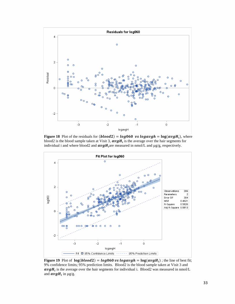
Figure 18 Plot of the residuals for (𝒃𝒍𝒐𝒐𝒅𝟐) = 𝒍𝒐𝒈𝟎𝟔𝟎 𝒗𝒔 𝒍𝒐𝒈𝒂𝒗𝒈𝒉 = 𝐥𝐨𝐠 (𝒂𝒗𝒈𝑯𝒊), where

blood2 is the blood sample taken at Visit 3, 𝒂𝒗𝒈𝑯𝒊 is the average over the hair segments for

individual i and where blood2 and 𝒂𝒗𝒈𝑯𝒊are measured in nmol/L and µg/g, respectively.

Figure 19 Plot of 𝐥𝐨𝐠(𝒃𝒍𝒐𝒐𝒅𝟐) = 𝒍𝒐𝒈𝟎𝟔𝟎 𝒗𝒔 𝒍𝒐𝒈𝒂𝒗𝒈𝒉 = 𝐥𝐨𝐠 (𝒂𝒗𝒈𝑯𝒊) ; the line of best fit;

9% confidence limits; 95% prediction limits. Blood2 is the blood sample taken at Visit 3 and

𝒂𝒗𝒈𝑯𝒊 is the average over the hair segments for individual i. Blood2 was measured in nmol/L

and 𝒂𝒗𝒈𝑯𝒊 in µg/g.

34

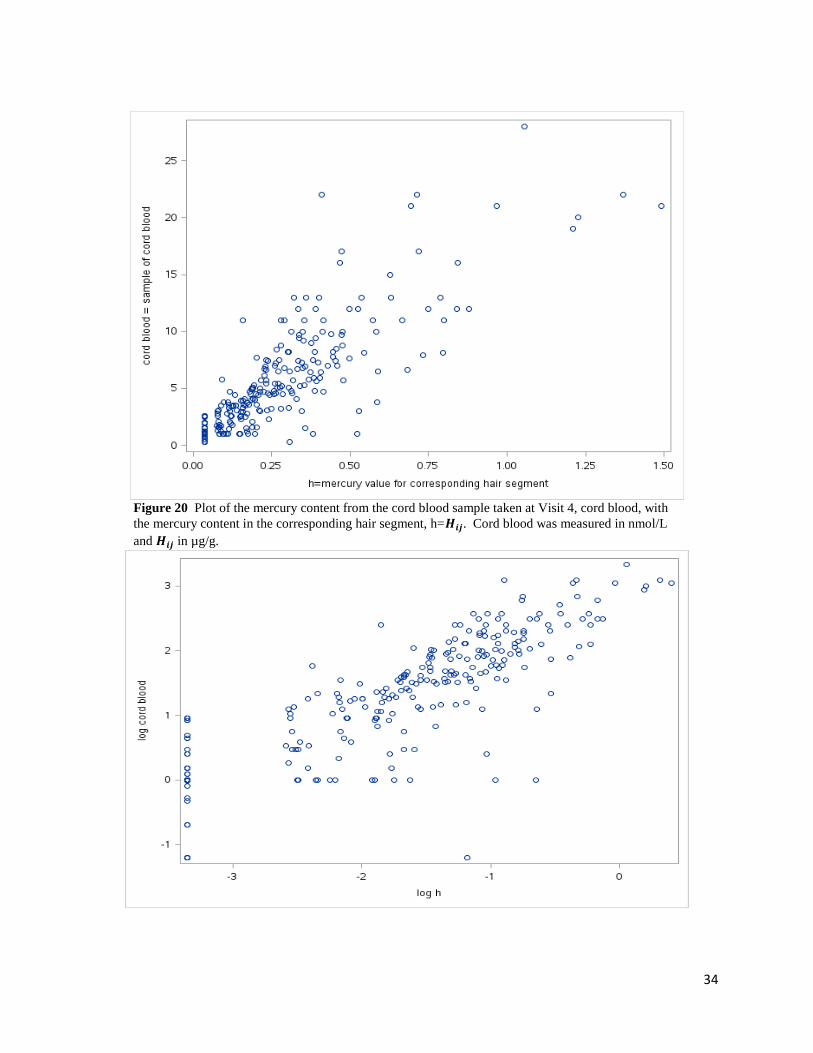
Figure 20 Plot of the mercury content from the cord blood sample taken at Visit 4, cord blood, with

the mercury content in the corresponding hair segment, h=𝑯𝒊𝒋. Cord blood was measured in nmol/L

and 𝑯𝒊𝒋 in µg/g.

35

Figure 21 Plot of the log of the cord blood sample taken at Visit 4 vs the log of the corresponding hair

segment, i.e. 𝐥𝐨𝐠(𝒄𝒐𝒓𝒅 𝒃𝒍𝒐𝒐𝒅) 𝒗𝒔 𝒍𝒐𝒈𝒉, where 𝒉 = 𝑯𝒊𝒋. Cord blood was measured in nmol/L and

𝑯𝒊𝒋 in µg/g.

Figure 22 Plot of the log of the cord blood sample taken at Visit 4 vs the log of the average of the hair

segments for a particular sample, 𝐥𝐨𝐠(𝒄𝒐𝒓𝒅 𝒃𝒍𝒐𝒐𝒅) 𝒗𝒔 𝒍𝒐𝒈𝒂𝒗𝒈𝒉, where 𝒍𝒐𝒈𝒂𝒗𝒈𝒉 = 𝐥𝐨𝐠 (𝒂𝒗𝒈𝑯𝒊).

Cord blood was measured in nmol/L and 𝒂𝒗𝒈𝑯𝒊 in µg/g.

36

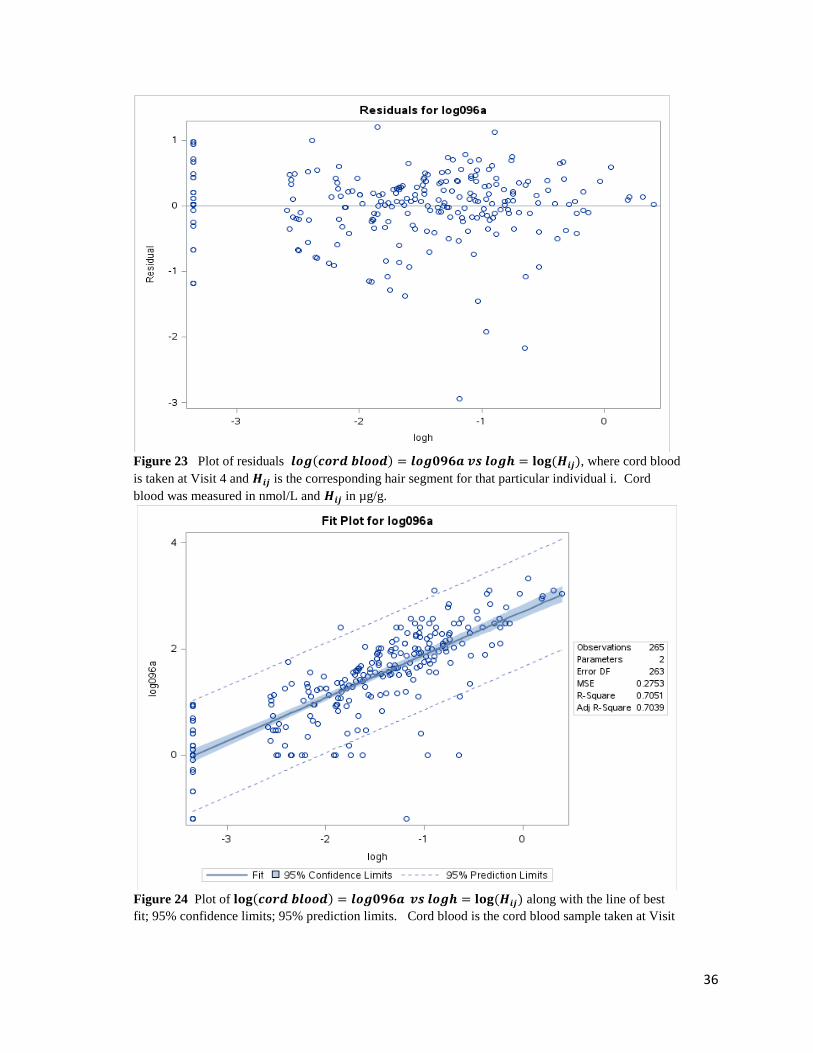
Figure 23 Plot of residuals 𝒍𝒐𝒈(𝒄𝒐𝒓𝒅 𝒃𝒍𝒐𝒐𝒅) = 𝒍𝒐𝒈𝟎𝟗𝟔𝒂 𝒗𝒔 𝒍𝒐𝒈𝒉 = 𝐥𝐨𝐠 (𝑯𝒊𝒋), where cord blood

is taken at Visit 4 and 𝑯𝒊𝒋 is the corresponding hair segment for that particular individual i. Cord

blood was measured in nmol/L and 𝑯𝒊𝒋 in µg/g.

Figure 24 Plot of 𝐥𝐨𝐠(𝒄𝒐𝒓𝒅 𝒃𝒍𝒐𝒐𝒅) = 𝒍𝒐𝒈𝟎𝟗𝟔𝒂 𝒗𝒔 𝒍𝒐𝒈𝒉 = 𝐥𝐨𝐠 (𝑯𝒊𝒋) along with the line of best

fit; 95% confidence limits; 95% prediction limits. Cord blood is the cord blood sample taken at Visit

37

4 and 𝑯𝒊𝒋 is the corresponding hair segment for individual i. Cord blood was measured in nmol/L and

𝑯𝒊𝒋 in µg/g.

Figure 25 Plot of the residuals for (𝒄𝒐𝒓𝒅 𝒃𝒍𝒐𝒐𝒅) = 𝒍𝒐𝒈𝟎𝟗𝟔𝒂 𝒗𝒔 𝒍𝒐𝒈𝒂𝒗𝒈𝒉 = 𝐥𝐨𝐠 (𝒂𝒗𝒈𝑯𝒊) ,

where cord blood is the cord blood sample taken at Visit 4 and 𝒂𝒗𝒈𝑯𝒊 is the average over the hair

segments for individual i. Cord blood was measured in nmol/L and 𝒂𝒗𝒈𝑯𝒊 in µg/g.

Figure 26 Plot of 𝐥𝐨𝐠(𝒄𝒐𝒓𝒅 𝒃𝒍𝒐𝒐𝒅) = 𝒍𝒐𝒈𝟎𝟗𝟔𝒂 𝒗𝒔 𝒍𝒐𝒈𝒂𝒗𝒈𝒉 = 𝐥𝐨𝐠 (𝒂𝒗𝒈𝑯𝒊); the line of best

fit; 9% confidence limits; 95% prediction limits. Cord blood is the cord blood sample taken at

38

Visit 4 and 𝒂𝒗𝒈𝑯𝒊 is the average over the hair segments for individual i. Cord blood was

measured in nmol/L and 𝒂𝒗𝒈𝑯𝒊 in µg/g.

Figure 27 Plot of the mercury content from the meconium sample taken at Visit 5a, meconium, with

the mercury content in the corresponding hair segment, h=𝑯𝒊𝒋. Meconium and 𝑯𝒊𝒋 were measured in

µg/g.

39

Figure 28 Plot of the log of the meconium sample taken at Visit 5a vs the log of the corresponding

hair segment, i.e. 𝐥𝐨𝐠(𝒎𝒆𝒄𝒐𝒏𝒊𝒖𝒎) 𝒗𝒔 𝒍𝒐𝒈𝒉, where 𝒉 = 𝑯𝒊𝒋. Meconium and 𝑯𝒊𝒋 were measured in

µg/g.

Figure 29 Plot of the log of the meconium sample taken at Visit 5a vs the log of the average of the

hair segments for a particular sample, 𝐥𝐨𝐠(𝒎𝒆𝒄𝒐𝒏𝒊𝒖𝒎) 𝒗𝒔 𝒍𝒐𝒈𝒂𝒗𝒈𝒉, where 𝒍𝒐𝒈𝒂𝒗𝒈𝒉 =𝐥𝐨𝐠 (𝒂𝒗𝒈𝑯𝒊) . Meconium and 𝒂𝒗𝒈𝑯𝒊 were measured in µg/g.

40

Figure 30 Plot of residuals 𝒍𝒐𝒈(𝒎𝒆𝒄𝒐𝒏𝒊𝒖𝒎) = 𝒍𝒐𝒈𝟏𝟐𝟐𝒂 𝒗𝒔 𝒍𝒐𝒈𝒉 = 𝐥𝐨𝐠 (𝑯𝒊𝒋), where

meconium is the meconium sample taken at Visit 5a and 𝑯𝒊𝒋 is the corresponding hair segment for

that particular individual i. Meconium and 𝑯𝒊𝒋 were measured in µg/g.

41

Figure 31 Plot of 𝐥𝐨𝐠(𝒎𝒆𝒄𝒐𝒏𝒊𝒖𝒎) = 𝒍𝒐𝒈𝟏𝟐𝟐𝒂 𝒗𝒔 𝒍𝒐𝒈𝒉 = 𝐥𝐨𝐠 (𝑯𝒊𝒋) along with the line of

best fit; 95% confidence limits; 95% prediction limits. Meconium is the meconium sample taken

at Visit 5a and 𝑯𝒊𝒋 is the corresponding hair segment for individual i. Meconium and 𝑯𝒊𝒋 were

measured in µg/g.

Figure 32 Plot of the residuals for 𝒍𝒐𝒈(𝒎𝒆𝒄𝒐𝒏𝒊𝒖𝒎) = 𝒍𝒐𝒈𝟏𝟐𝟐𝒂 𝒗𝒔 𝒍𝒐𝒈𝒂𝒗𝒈𝒉 = 𝐥𝐨𝐠 (𝒂𝒗𝒈𝑯𝒊)

where meconium is the meconium sample taken at Visit 5a and 𝒂𝒗𝒈𝑯𝒊 is the average over the hair

segments for individual i. Meconium and 𝒂𝒗𝒈𝑯𝒊 were measured in µg/g.

42

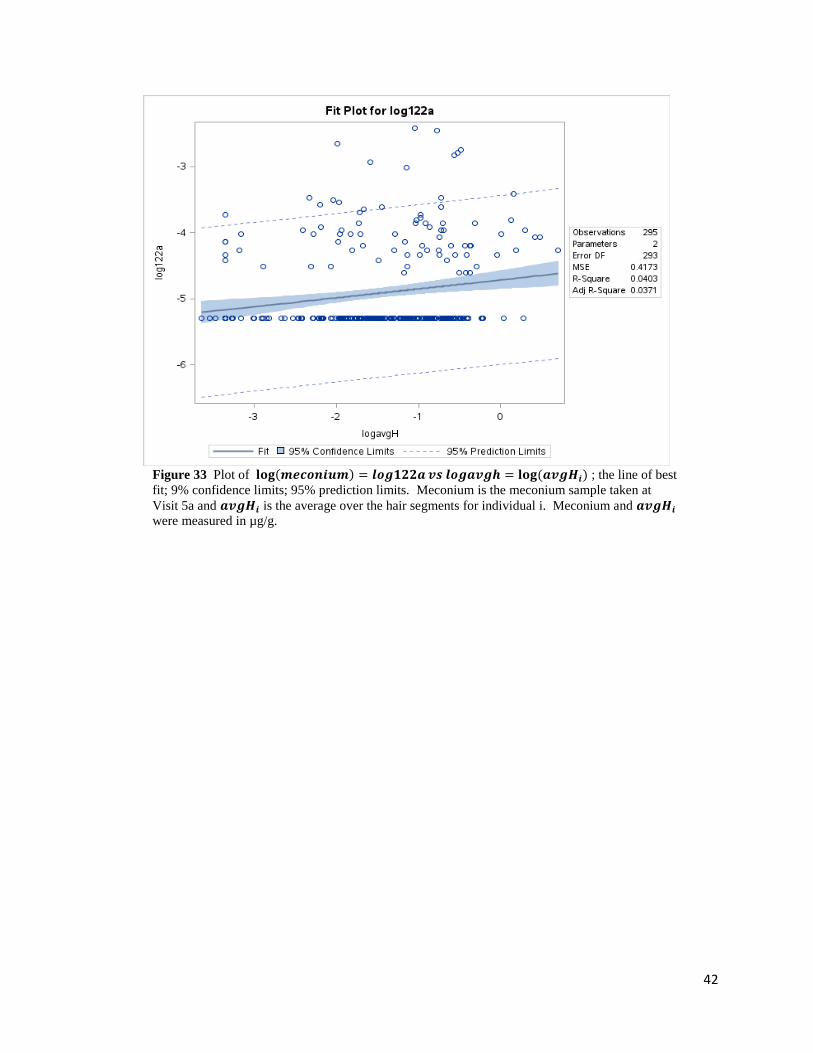
Figure 33 Plot of 𝐥𝐨𝐠(𝒎𝒆𝒄𝒐𝒏𝒊𝒖𝒎) = 𝒍𝒐𝒈𝟏𝟐𝟐𝒂 𝒗𝒔 𝒍𝒐𝒈𝒂𝒗𝒈𝒉 = 𝐥𝐨𝐠 (𝒂𝒗𝒈𝑯𝒊) ; the line of best

fit; 9% confidence limits; 95% prediction limits. Meconium is the meconium sample taken at

Visit 5a and 𝒂𝒗𝒈𝑯𝒊 is the average over the hair segments for individual i. Meconium and 𝒂𝒗𝒈𝑯𝒊

were measured in µg/g.