Detection of Human Fall Using Floor Vibration and Multi

sensors

Article

Detection of Human Fall Using Floor Vibration andMulti-Features Semi-Supervised SVM

Chengyin Liu 1, Zhaoshuo Jiang 2,*, Xiangxiang Su 1, Samuel Benzoni 2 and Alec Maxwell 2

1 Department of Civil and Environmental Engineering, Harbin Institute of Technology,Shenzhen 518055, China

2 School of Engineering, San Francisco State University, San Francisco, CA 94132, USA* Correspondence: [email protected]; Tel.: +1-415-338-7741

Received: 4 August 2019; Accepted: 26 August 2019; Published: 28 August 2019��

Abstract: Human falls are the premier cause of fatal and nonfatal injuries among older adults.The health outcome of a fall event is largely dependent on rapid response and rescue of the fallenelder. Being able to provide an accurate and fast fall detection will dramatically improve the healthoutcomes of the older population and reduce the associated healthcare cost after a fall. To achieve thegoal, a multi-features semi-supervised support vector machines (MFSS-SVM) algorithm utilizingmeasurements from structural floor vibration obtained through accelerometers is proposed in thisstudy to detect falling events with limited labeled samples. In this MFSS-SVM algorithm, the peakvalue, energy, and correlation coefficient of the accelerometer signal are used as classification features.The performance of the proposed algorithm was validated with laboratory experiments amongactivities including falling, walking, free jumping, rhythmic jumping, bag dropping, and ball dropping.To further illustrate the performance of the algorithm, a benchmark database was adopted andexpanded to test its ability to accurately identify falling, compared with the algorithm used in thebenchmark study. Results show that by using the proposed algorithm, the falling events can beidentified with high accuracy and confidence, even with small training datasets and test nodes.

Keywords: falling detection; fall loading model; floor vibration; multi-features semi-supervisedsupport vector machines; benchmark problem

1. Introduction

The world’s population is growing older. According to the recent report from the Census Bureau,it is estimated that 1.6 billion (17%) of the total 9.4 billion population will be 65 and older in 2050 [1].Human falls are the premier cause of fatal and nonfatal injuries among older adults, which affect onein three aged 65 and over half of those aged 80+ every year [2,3]. The health outcome of a fall event islargely dependent on rapid response and rescue of the fallen elder.

Based on whether the user’s interference is necessary, current fall detection methods can beclassified into two categories: user-dependent and user-independent. The user-dependent methodseither use wearable devices (e.g., pendant, watch, clip, bracelet, or ring) to track rapid changes in itsorientation or rely on users themselves to report the emergency of fall by interacting (e.g., pressing) thewearable device [4–9]. These options suffer from limitations such as getting the person to wear the deviceor false-positive detection (e.g., a fall is incorrectly identified when no fall occurs) due to user’s abruptmovement. Research on fall detection through user-independent means often uses infrared camerasto monitor users’ behavior and detect fall events with computer vision techniques [10,11]. However,the use of cameras would meet with resistance as residents have a feeling of “being watched” [12].Progress toward new methods without cameras has been made through the use of accelerometersensors mounted on the structure to capture floor vibration for human activities detection [13–16].

Sensors 2019, 19, 3720; doi:10.3390/s19173720 www.mdpi.com/journal/sensors

http://www.mdpi.com/journal/sensors

http://www.mdpi.com

http://dx.doi.org/10.3390/s19173720

http://www.mdpi.com/journal/sensors

http://www.mdpi.com/1424-8220/19/17/3720?type=check_update&version=3

Sensors 2019, 19, 3720 2 of 20

For example, Madarshahian et al. [13] proposed a benchmark problem to promote exploration offloor vibrations to classify human activities. The benchmark problem provided 16,100 records offloor vibrations induced by human activities including bouncing a ball, jumping, and dropping abag and included an example solution with an algorithm based on the difference of the accelerationautocorrelations. Poston et al. [14] attempted to use measurements of footstep-generated vibrationsfrom accelerometers originally deployed to measure a building’s structural dynamics to locateindividuals moving within a building. In this study, a specific time-of-arrival estimation algorithmsuited to the type of footstep-to-sensor interaction was developed to work with the data collectedthrough 12 single-axis accelerometers mounted underneath the building floor.

For fall detection, in particular, Alwan et al. [12] utilized a special piezoelectric sensor coupled tothe floor surface using a mass and spring arrangement together with battery-powered preprocessingelectronics to capture the floor vibration. The authors identified the falling events through passivelymonitoring the floor vibration patterns. Zigel et al. [15] used floor vibration and sound sensingin sequence with signal processing and a pattern recognition algorithm to detect falling events.In general, the detection algorithms can be categorized into threshold-based and classifier-based.In threshold-based algorithms, thresholds are set for various chosen features, to which the measuredvalues will be compared during the detection phase. Due to large variations and uncertainties inactual usages, such as structural configurations, impact locations, and the distance between the impactand the sensors, the thresholds may need to be modified dramatically for different implementations.This creates challenges for determining a set of thresholds for all scenarios. With the advancementof technologies and computational power, the use of classifiers for various applications has receivedsignificant attention in recent years. Classifiers, such as k-nearest neighbors [17,18], support vectormachines [19,20], naïve Bayes [21], artificial neural networks [22,23], hidden Markov model [24],and fuzzy logic [25], have been investigated to improve the identification accuracy. One of thechallenges these classifier-based methods face is the need for a large training dataset.

In this study, a multi-features semi-supervised support vector machines (MFSS-SVM) algorithmwith a radial basis function kernel is proposed to identify falling events through the use of accelerometermeasurements from floor vibration. The proposed MFSS-SVM algorithm makes use of the unlabeleddatasets and multi-feature classifier integrated from several base classifiers during the training process,resulting in an improved performance with fewer required training datasets and shorter training time.To generate the fall datasets, highly-imitated dummies were utilized to mimic human falling. This paperfirst provides a brief review of SVM, semi-supervised SVM, and multi-features semi-supervised SVM,followed by the introduction of the proposed algorithm. Next, the performance of the proposedalgorithm was investigated with laboratory testing and through an expanded benchmark database.

2. Proposed Fall Detection Algorithm

2.1. SVM Classifier

To correctly detect a human fall, a pattern recognition needs to be performed to differentiatethe fall from other daily activities, such as walking, jumping, and impact from an object falling.After extracting the desired information from the raw data, a classifier is typically designed anddeveloped to categorize the different activities during the pattern recognition process. Among variousclassifiers, neural networks and SVM are two popular strategies for supervised machine learning andclassification. The neural network is widely used, given its ability to learn and model both simple andcomplex relationships. However, selecting the appropriate features may require extensive expertise,and the time needed to train the model could hinder its usage. The SVM has been shown to be asuperior method for binary classification [26,27]. For instance, Davis et al. [28] studied the use of SVMsto classify floor vibration signals to differentiate signals of interest.

Typically, the SVM performs the task of binary classification by mapping input vectors into ahyperplane, a high-dimensional feature space, that is constructed to separate input vectors [29]. If it

Sensors 2019, 19, 3720 3 of 20

exists, this hyperplane maximizes the margin between different classes, and thus, the well-knowngeneralization measure called Vapnik–Chervonenkis dimension [30]. Simultaneously, the hyperplaneminimizes the empirical error, which is the error committed by the training data. Equation (1) isa mathematical representation that can be used to describe the optimization problem of a generalSVM classification.

minimize{12

w·w + Cl∑

i=1

ξi}, subject to yi(w·ϕ(xi) + b) ≥ 1− ξi, (i = 1, 2, 3, . . . l), (1)

where C is the penalty parameter and ξi is the slack variable, a parameter to handle inseparable data.Generally, maximizing the classification margin and minimizing the misclassifying rate minimizes

Equation (1). The parameter C controls the trade-off between the size of the margin and the penalty ofslack variables, a measure of the error. yi (i from 1 to l) ∈ ±1 represents the class labels for differenttraining cases and xi represents the independent variables. ϕ is the kernel function used to transformdata from the input vectors into the feature spaces. Linear kernel, polynomial kernel, and radial basisfunction (RBF) kernel are the three kinds of functions commonly used in practice. In this paper, the RBFis adopted as the kernel functions of SVM.

2.2. Semi-Supervised SVM

To the best of the authors’ knowledge, the first semi-supervised SVM method was proposed byJoachims [31] for text classification purpose, and later improved approaches have been presentedin the literature for multiple purposes, such as image/text classification [32–34] and vison-based falldetection [35–37]. While traditional SVM classifiers utilize a general decision function with a setof labeled training samples, a semi-supervised SVM iteratively takes advantage of the unlabeleddatasets and simultaneously considers all the available labeled and unlabeled samples to minimizethe classification errors. In the initial iteration, an SVM model is first trained using Equation (1)and pseudo-labels are assigned to the unlabeled datasets. Some of these newly labeled samples arefurther chosen as semi-labeled samples based on a given criterion. From the theory of SVM, only thesamples within the margins (i.e., the samples that have the decision function value y between ±1)have influences on the position of the hyperplane that separates the different classification categories.Among these samples, the ones closest to the margins (i.e., y = ±1) have the highest probabilityof being correctly labeled. Thus, the unlabeled samples that are closest to the margins are usuallyadded to the training dataset, resulting in a hybrid dataset with labeled and semi-labeled samples.The optimization problem in Equation (1) now can be converted to:

minimize{

12‖W‖

2 + Cn∑

l=1ξl + C∗

d∑u=1

ξ∗u

}yl(WT·Φ(X) + b

)≥ 1− ξl, ξl ≥ 0, l = 1, · · · , n

y∗u(WT·Φ(X∗) + b

)≥ 1− ξ∗u, ξ∗u ≥ 0, u = 1, · · · , d

(2)

where ξl and ξ∗u are the slack variables for the labeled and semi-labeled samples, respectively. C and C∗

are the penalty parameters for the labeled and semi-labeled samples, respectively.With the new hybrid training set, the semi-supervised SVM is retrained iteratively until it reaches

a stopping criterion (e.g., maximum number of iterations). At each iteration, new semi-labeled samplesobtained in the previous iteration are added to the training dataset. The semi-labeled samples whoselabel has changed from the previous iteration are removed from the new semi-labeled dataset and putback to the unlabeled dataset.

Sensors 2019, 19, 3720 4 of 20

2.3. Multi-Feature Semi-Supervised SVM Framework for Human Fall Detection

In this paper, the MFSS-SVM is proposed to specifically tackle the human falling classificationproblem. In particular, compared with the traditional semi-supervised SVM, the unique characteristicof the MFSS-SVM lies in its multi-feature classifier integrated from several base classifiers. Researchesin the previous studies have shown that better classification performance can be achieved for greaterdifference among the base classifiers. In addition to the common features of the time-domainacceleration signals, such as the peak value, two features, namely energy and sensor correlationcoefficient, were selected to identify the vibration characteristics of falling in the records.

(1) Peak value: This feature determines the maximum absolute value of the signals. It can beexpressed as

Amax = max(∣∣∣a(t)∣∣∣), (3)

where a(t) is the time history of the acceleration signal.(2) Energy: The energy metric attempts to characterize the strength of the recorded signal. It can be

calculated by integrating the area under the time history of the acceleration signal.

E =

∫ ∣∣∣a(t)∣∣∣dt. (4)

(3) Sensor correlation coefficient: This metric serves as an indication of how close the correlationbetween two different acceleration signals and can be described as

ρa1a2=

Cov(a1(t), a2(t))√D(a1(t))

√D(a2(t))

(5)

where a1(t) and a2(t) are the acceleration signals from two accelerometers; Cov() is the correlationdeviation of a1(t) and a2(t); D() is the standard deviation. It is expected that, by takingconsideration of the sensor correlations, environmental random effects are reduced to betterrepresent the event.

Compared to statistical features, such as standard deviation, mean value, and Root Mean Square,these proposed features were identified to have higher divergence in a preliminary study and thusadopted in this study to be extracted as classification features in the data pre-processing.

The tri-training cooperative training strategy [38,39] was applied to the three different baseclassifiers obtained through the three extracted features defined above [40–42], after which anagent-based statistical scheme, the majority-vote model [43], was utilized to integrate them to form theMFSS-SVM classifier. The labeling rate of the MFSS-SVM was also investigated in this study to strikea balance between accuracy and speed, as a high number of labeling rate increases computationalburden for real-time MFSS-SVM classification.

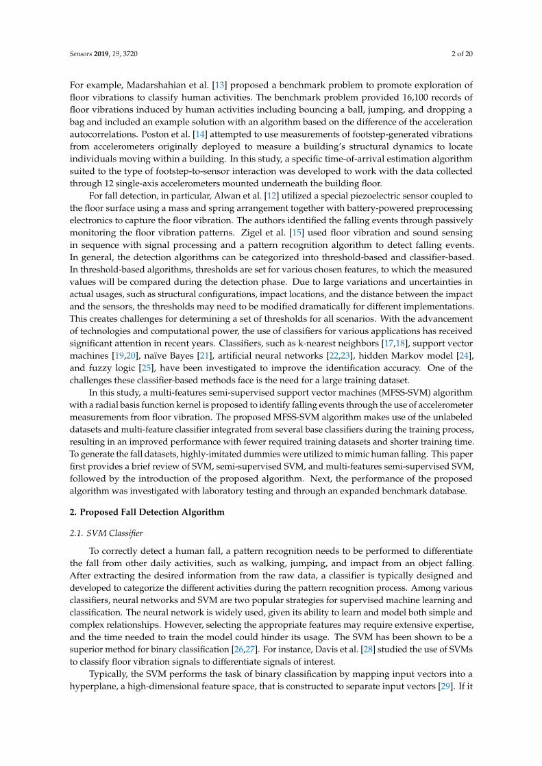
The proposed MFSS-SVM framework, composed of the training and testing phases,is demonstrated in Figure 1. The steps for implementing the framework can be described as

Step 1. Three feature vectors are calculated by extracting peak value, energy, and sensor correlationcoefficients from the training samples.

Step 2. The RBF classifier is employed in SVM training on these three extracted features.Step 3. The tri-training cooperative training strategy is applied to semi-supervised learning.Step 4. The majority-vote technique is applied to integrate three different basic classifiers resulting

from the previous step to form the MFSS-SVM classifier.Step 5. The feature vectors of peak value, energy, and sensor correlation coefficients of the testing

samples are extracted.Step 6. The extracted feature vectors from the testing samples are input into the trained MFSS-SVM

classifier for classification, and the fall detection accuracy is calculated.

Sensors 2019, 19, 3720 5 of 20

Sensors 2019, 19, x FOR PEER REVIEW 5 of 19

Figure 1. The proposed multi-features semi-supervised support vector machines (MFSS-SVM) framework.

3. Experimental Verification

3.1. Experiment Setup

To test the proposed MFSS-SVM algorithm, experiments were performed in the intelligent structural hazard mitigation laboratory (iSHM Lab) at San Francisco State University (Figure 2) to collect vibration signals of human falling and other activities in daily life. Four PCB (PCB Piezotronics, Depew, NY, USA) high sensitivity uniaxial accelerometers (Model: 393B31; Sensitivity: 10.0 V/g; Frequency Range: 0.1 to 200 Hz) were used to measure the floor vibration signals. Considering the laboratory layout and the structural configuration of the slabs (e.g., underneath beams), three accelerometers were placed near the wall, and one was set near the center of the floor as shown in Figure 3. A National Instrument cDAQ-9171 (32-bit resolution) with a NI 9234 input module (24-bit resolution) was used as the data acquisition system. One thousand, six hundred and fifty-two hertz was chosen as the sampling frequency as it is the lowest sampling rate of the data acquisition system, and it is well above the frequency range of the human activities of interest.

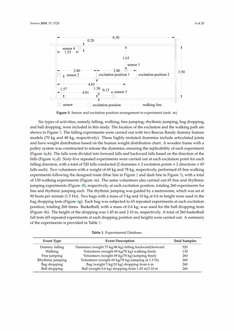
Six types of activities, namely falling, walking, free jumping, rhythmic jumping, bag dropping, and ball dropping, were included in this study. The location of the excitation and the walking path are shown in Figure 3. The falling experiments were carried out with two Rescue Randy dummy human models (70 kg and 48 kg, respectively). These highly-imitated dummies include articulated joints and have weight distribution based on the human weight distribution chart. A wooden frame with a pulley system was constructed to release the dummies, ensuring the replicability of each experiment (Figure 4a,b). The falls were divided into forward falls and backward falls based on the direction of the falls (Figure 4c,d). Sixty-five repeated experiments were carried out at each excitation point for each falling direction, with a total of 520 falls conducted (2 dummies × 2 excitation points × 2 directions × 65 falls each). Two volunteers with a weight of 69 kg and 78 kg, respectively, performed 65 free walking experiments following the designed route (blue line in Figure 2 and dash line in Figure 3), with a total of 130 walking experiments (Figure 4e). The same volunteers also carried out 65 free and rhythmic jumping experiments (Figure 4f), respectively, at each excitation position, totaling 260 experiments for free and rhythmic jumping each. The rhythmic jumping was guided by a metronome, which was set at 90 beats per minute (1.5 Hz). Two bags with a mass of 5 kg and 10 kg at 0.6 m height were used in the bag dropping tests (Figure 4g). Each bag was subjected to 65 repeated experiments at each excitation position, totaling 260 times. Basketball, with a mass of 0.6 kg, was used

Figure 1. The proposed multi-features semi-supervised support vector machines (MFSS-SVM) framework.

3. Experimental Verification

3.1. Experiment Setup

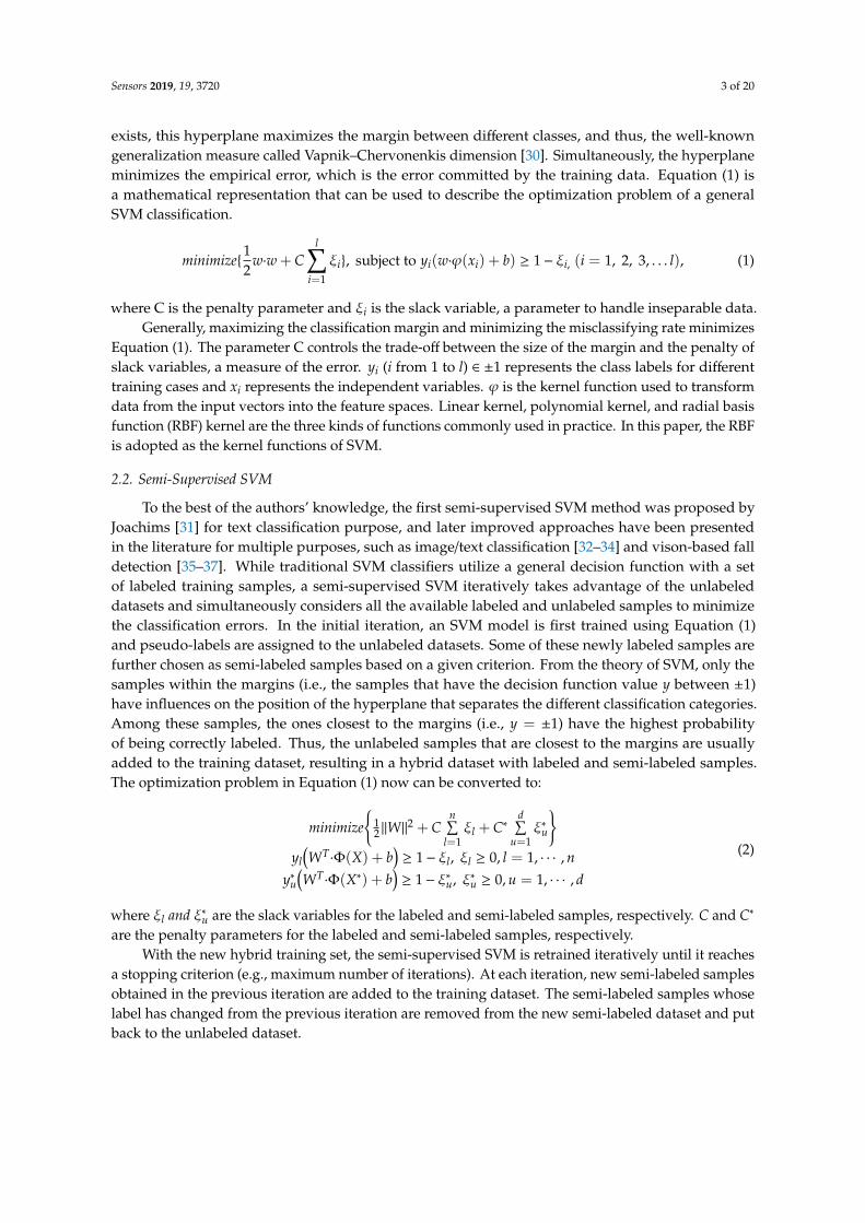
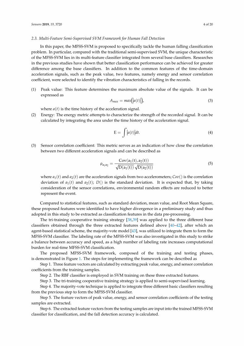
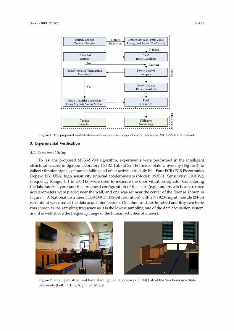
To test the proposed MFSS-SVM algorithm, experiments were performed in the intelligentstructural hazard mitigation laboratory (iSHM Lab) at San Francisco State University (Figure 2) tocollect vibration signals of human falling and other activities in daily life. Four PCB (PCB Piezotronics,Depew, NY, USA) high sensitivity uniaxial accelerometers (Model: 393B31; Sensitivity: 10.0 V/g;Frequency Range: 0.1 to 200 Hz) were used to measure the floor vibration signals. Consideringthe laboratory layout and the structural configuration of the slabs (e.g., underneath beams), threeaccelerometers were placed near the wall, and one was set near the center of the floor as shown inFigure 3. A National Instrument cDAQ-9171 (32-bit resolution) with a NI 9234 input module (24-bitresolution) was used as the data acquisition system. One thousand, six hundred and fifty-two hertzwas chosen as the sampling frequency as it is the lowest sampling rate of the data acquisition system,and it is well above the frequency range of the human activities of interest.


for the ball dropping tests (Figure 4h). The height of the dropping was 1.45 m and 2.10 m, respectively. A total of 260 basketball fall tests (65 repeated experiments at each dropping position and height) were carried out. A summary of the experiments is provided in Table 1.

Figure 2. Intelligent structural hazard mitigation laboratory (iSHM) Lab at the San Francisco State University (Left: Picture; Right: 3D Model).

sensor excitation position

1.55

0.20

1.574.85

1.30

2.80 2.80

4.01 0.15

excitation position 2excitation position 1sensor 2

sensor 4

sensor 3

sensor 11.63

3.50

8.30

walking line Figure 3. Sensor and excitation position arrangement in experiment (unit: m).

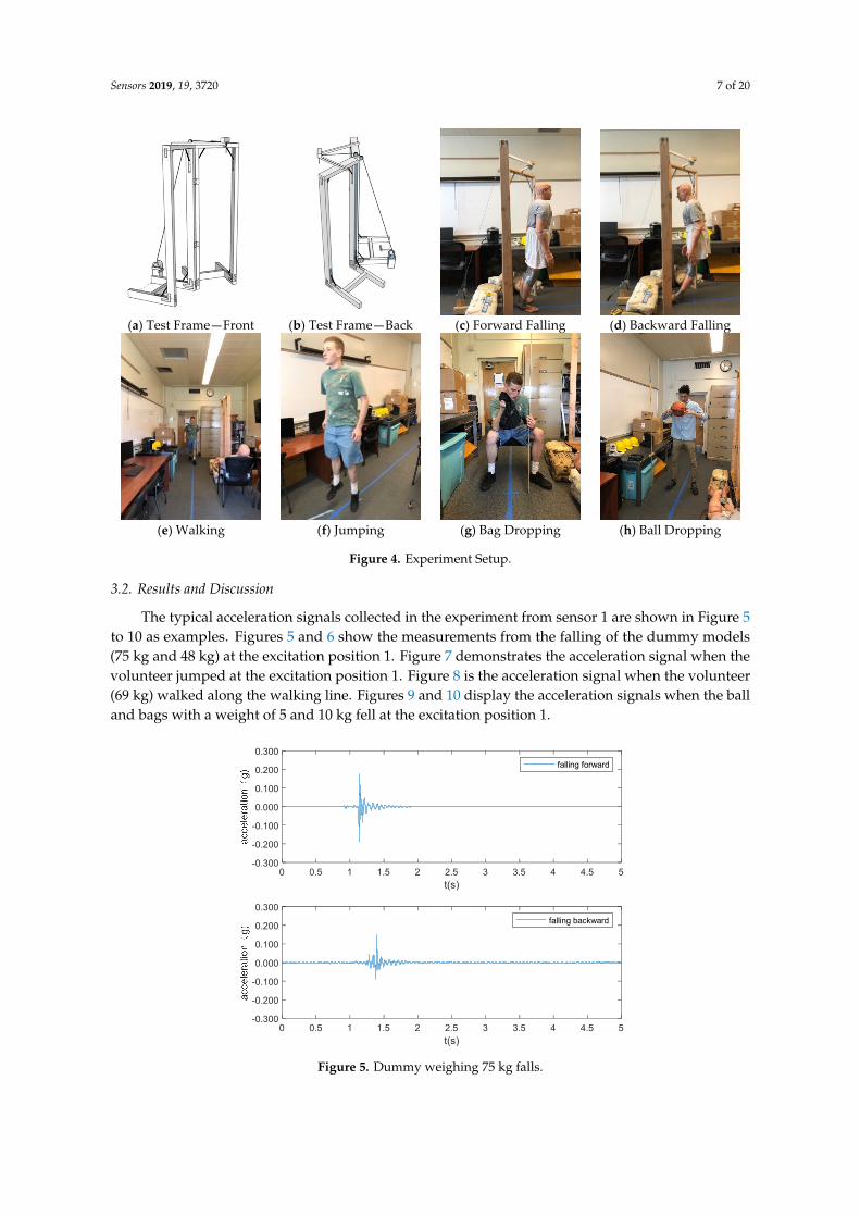
(a) Test Frame—Front (b) Test Frame—Back (c) Forward Falling (d) Backward Falling

(e) Walking (f) Jumping (g) Bag Dropping (h) Ball Dropping

Figure 4. Experiment Setup.

Figure 2. Intelligent structural hazard mitigation laboratory (iSHM) Lab at the San Francisco StateUniversity (Left: Picture; Right: 3D Model).

Sensors 2019, 19, 3720 6 of 20





1.55

0.20

1.574.85

1.30

2.80 2.80

4.01 0.15


sensor 4

sensor 3

sensor 11.63

3.50

8.30




Figure 4. Experiment Setup.

Figure 3. Sensor and excitation position arrangement in experiment (unit: m).

Six types of activities, namely falling, walking, free jumping, rhythmic jumping, bag dropping,and ball dropping, were included in this study. The location of the excitation and the walking path areshown in Figure 3. The falling experiments were carried out with two Rescue Randy dummy humanmodels (70 kg and 48 kg, respectively). These highly-imitated dummies include articulated jointsand have weight distribution based on the human weight distribution chart. A wooden frame with apulley system was constructed to release the dummies, ensuring the replicability of each experiment(Figure 4a,b). The falls were divided into forward falls and backward falls based on the direction of thefalls (Figure 4c,d). Sixty-five repeated experiments were carried out at each excitation point for eachfalling direction, with a total of 520 falls conducted (2 dummies × 2 excitation points × 2 directions × 65falls each). Two volunteers with a weight of 69 kg and 78 kg, respectively, performed 65 free walkingexperiments following the designed route (blue line in Figure 2 and dash line in Figure 3), with a totalof 130 walking experiments (Figure 4e). The same volunteers also carried out 65 free and rhythmicjumping experiments (Figure 4f), respectively, at each excitation position, totaling 260 experiments forfree and rhythmic jumping each. The rhythmic jumping was guided by a metronome, which was set at90 beats per minute (1.5 Hz). Two bags with a mass of 5 kg and 10 kg at 0.6 m height were used in thebag dropping tests (Figure 4g). Each bag was subjected to 65 repeated experiments at each excitationposition, totaling 260 times. Basketball, with a mass of 0.6 kg, was used for the ball dropping tests(Figure 4h). The height of the dropping was 1.45 m and 2.10 m, respectively. A total of 260 basketballfall tests (65 repeated experiments at each dropping position and height) were carried out. A summaryof the experiments is provided in Table 1.

Table 1. Experimental Database.

Event Type Event Description Total Samples

Dummy falling Dummies (weight 75 kg/48 kg) falling backward/forward 520Walking Volunteers (weight 69 kg/78 kg) walking freely 130

Free jumping Volunteers (weight 69 kg/78 kg) jumping freely 260Rhythmic jumping Volunteers (weight 69 kg/78 kg) jumping at 1.5 Hz 260

Bag dropping Bag (weight 5 kg/10 kg) dropping from 6 m 260Ball dropping Ball (weight 0.6 kg) dropping from 1.45 m/2.10 m 260

Sensors 2019, 19, 3720 7 of 20





1.55

0.20

1.574.85

1.30

2.80 2.80

4.01 0.15


sensor 4

sensor 3

sensor 11.63

3.50

8.30




Figure 4. Experiment Setup. Figure 4. Experiment Setup.

3.2. Results and Discussion

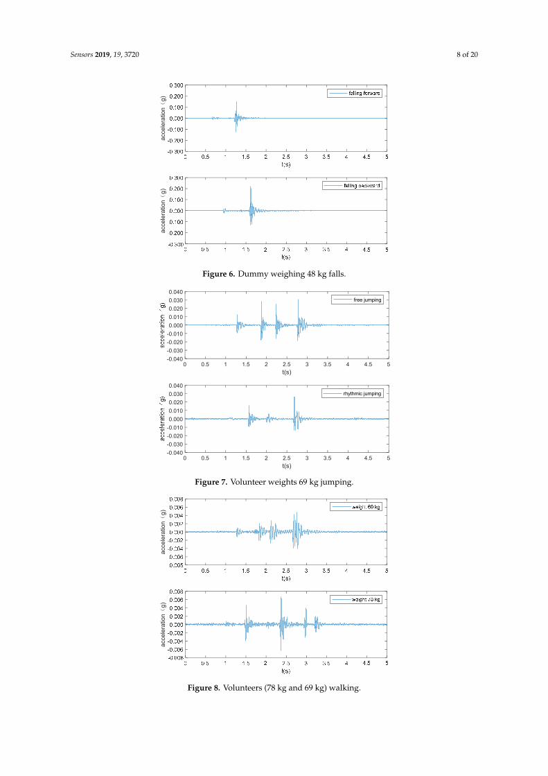
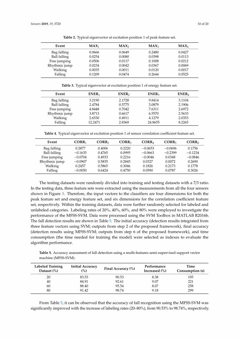
The typical acceleration signals collected in the experiment from sensor 1 are shown in Figure 5to 10 as examples. Figures 5 and 6 show the measurements from the falling of the dummy models(75 kg and 48 kg) at the excitation position 1. Figure 7 demonstrates the acceleration signal when thevolunteer jumped at the excitation position 1. Figure 8 is the acceleration signal when the volunteer(69 kg) walked along the walking line. Figures 9 and 10 display the acceleration signals when the balland bags with a weight of 5 and 10 kg fell at the excitation position 1.




Dummy falling Dummies (weight 75 kg/48 kg) falling backward/forward 520

Walking Volunteers (weight 69 kg/78 kg) walking freely 130

Free jumping Volunteers (weight 69 kg/78 kg) jumping freely 260

Rhythmic jumping Volunteers (weight 69 kg/78 kg) jumping at 1.5 Hz 260

Bag dropping Bag (weight 5 kg/10 kg) dropping from 6 m 260

Ball dropping Ball (weight 0.6 kg) dropping from 1.45 m/2.10 m 260


The typical acceleration signals collected in the experiment from sensor 1 are shown in Figure 5 to 10 as examples. Figures 5 and 6 show the measurements from the falling of the dummy models (75 kg and 48 kg) at the excitation position 1. Figure 7 demonstrates the acceleration signal when the volunteer jumped at the excitation position 1. Figure 8 is the acceleration signal when the volunteer (69 kg) walked along the walking line. Figures 9 and 10 display the acceleration signals when the ball and bags with a weight of 5 and 10 kg fell at the excitation position 1.

Figure 5. Dummy weighing 75 kg falls.


0 0.5 1 1.5 2 2.5 3 3.5 4 4.5 5t(s)

-0.300

-0.200

-0.100

0.000

0.100

0.200

0.300falling forward

0 0.5 1 1.5 2 2.5 3 3.5 4 4.5 5t(s)

-0.300

-0.200

-0.100

0.000

0.100

0.200

0.300falling backward

acce

lera

tion（

g)ac

cele

ratio

n（g)


Sensors 2019, 19, 3720 8 of 20




Dummy falling Dummies (weight 75 kg/48 kg) falling backward/forward 520

Walking Volunteers (weight 69 kg/78 kg) walking freely 130

Free jumping Volunteers (weight 69 kg/78 kg) jumping freely 260

Rhythmic jumping Volunteers (weight 69 kg/78 kg) jumping at 1.5 Hz 260

Bag dropping Bag (weight 5 kg/10 kg) dropping from 6 m 260

Ball dropping Ball (weight 0.6 kg) dropping from 1.45 m/2.10 m 260


The typical acceleration signals collected in the experiment from sensor 1 are shown in Figure 5 to 10 as examples. Figures 5 and 6 show the measurements from the falling of the dummy models (75 kg and 48 kg) at the excitation position 1. Figure 7 demonstrates the acceleration signal when the volunteer jumped at the excitation position 1. Figure 8 is the acceleration signal when the volunteer (69 kg) walked along the walking line. Figures 9 and 10 display the acceleration signals when the ball and bags with a weight of 5 and 10 kg fell at the excitation position 1.



0 0.5 1 1.5 2 2.5 3 3.5 4 4.5 5t(s)

-0.300

-0.200

-0.100

0.000

0.100

0.200

0.300falling forward

0 0.5 1 1.5 2 2.5 3 3.5 4 4.5 5t(s)

-0.300

-0.200

-0.100

0.000

0.100

0.200

0.300falling backward

acce

lera

tion（

g)ac

cele

ratio

n（g)



Figure 7. Volunteer weights 69 kg jumping.

Figure 8. Volunteers (78 kg and 69 kg) walking.

Figure 9. Ball (0.6 kg) drops.

0 0.5 1 1.5 2 2.5 3 3.5 4 4.5 5t(s)

-0.040-0.030-0.020-0.0100.0000.0100.0200.0300.040

free jumping

0 0.5 1 1.5 2 2.5 3 3.5 4 4.5 5t(s)

-0.040-0.030-0.020-0.0100.0000.0100.0200.0300.040

rhythmic jumping

acce

lera

tion（

g)ac

cele

ratio

n（g)

0 0.5 1 1.5 2 2.5 3 3.5 4 4.5 5t(s)

-0.040-0.030-0.020-0.0100.0000.0100.0200.0300.040

drop height 1.45 m

0 0.5 1 1.5 2 2.5 3 3.5 4 4.5 5t(s)

-0.040-0.030-0.020-0.0100.0000.0100.0200.0300.040

drop height 2.10 m






0 0.5 1 1.5 2 2.5 3 3.5 4 4.5 5t(s)

-0.040-0.030-0.020-0.0100.0000.0100.0200.0300.040

free jumping

0 0.5 1 1.5 2 2.5 3 3.5 4 4.5 5t(s)

-0.040-0.030-0.020-0.0100.0000.0100.0200.0300.040

rhythmic jumping

acce

lera

tion（

g)ac

cele

ratio

n（g)

0 0.5 1 1.5 2 2.5 3 3.5 4 4.5 5t(s)

-0.040-0.030-0.020-0.0100.0000.0100.0200.0300.040

drop height 1.45 m

0 0.5 1 1.5 2 2.5 3 3.5 4 4.5 5t(s)

-0.040-0.030-0.020-0.0100.0000.0100.0200.0300.040

drop height 2.10 m


Sensors 2019, 19, 3720 9 of 20





0 0.5 1 1.5 2 2.5 3 3.5 4 4.5 5t(s)

-0.040-0.030-0.020-0.0100.0000.0100.0200.0300.040

free jumping

0 0.5 1 1.5 2 2.5 3 3.5 4 4.5 5t(s)

-0.040-0.030-0.020-0.0100.0000.0100.0200.0300.040

rhythmic jumping

acce

lera

tion（

g)ac

cele

ratio

n（g)

0 0.5 1 1.5 2 2.5 3 3.5 4 4.5 5t(s)

-0.040-0.030-0.020-0.0100.0000.0100.0200.0300.040

drop height 1.45 m

0 0.5 1 1.5 2 2.5 3 3.5 4 4.5 5t(s)

-0.040-0.030-0.020-0.0100.0000.0100.0200.0300.040

drop height 2.10 m



Figure 10. Bag (5 kg and 10 kg) drops.

The feature sets of peak value, energy, and sensor correlation coefficient were obtained from the experimental database. Each feature set contains 520 events of falling data and 1,170 events of other activities data. Typical feature vectors of various events at excitation position 1 are shown in Tables 2–4. Note that these results are merely one example among the large datasets, and they do not represent the statistical results.

Table 2. Typical eigenvector at excitation position 1 of peak feature set.

Event 𝐌𝐀𝐗𝟏 𝐌𝐀𝐗𝟐 𝐌𝐀𝐗𝟑 𝐌𝐀𝐗𝟒 Bag falling 0.0666 0.0649 0.2480 0.0427 Ball falling 0.0254 0.0080 0.0398 0.0113

Free jumping 0.0506 0.0117 0.1008 0.0212 Rhythmic jump 0.0234 0.0042 0.0367 0.0069

Walking 0.0035 0.0011 0.0120 0.0017 Falling 0.1209 0.0474 0.2644 0.0525

Table 3. Typical eigenvector at excitation position 1 of energy feature set.

Event 𝐄𝐍𝐄𝐑𝟏 𝐄𝐍𝐄𝐑𝟐 𝐄𝐍𝐄𝐑𝟑 𝐄𝐍𝐄𝐑𝟒 Bag falling 3.2190 2.1728 9.8414 3.1104 Ball falling 2.4784 0.5775 3.0879 2.1906

Free jumping 4.8448 0.7042 7.6311 2.6972 Rhythmic jump 3.8713 0.6617 6.5570 2.5633

Walking 2.6530 0.4911 4.1279 2.0353 Falling 12.2471 2.8369 24.8655 8.2265

Table 4. Typical eigenvector at excitation position 1 of sensor correlation coefficient feature set.

Event 𝐂𝐎𝐑𝐑𝟏 𝐂𝐎𝐑𝐑𝟐 𝐂𝐎𝐑𝐑𝟑 𝐂𝐎𝐑𝐑𝟒 𝐂𝐎𝐑𝐑𝟓 𝐂𝐎𝐑𝐑𝟔 Bag falling 0.2877 0.4006 0.2220 −0.0653 −0.0696 0.1756 Ball falling −0.1635 0.4765 0.0995 −0.0663 −0.2399 −0.1234

Free jumping −0.0704 0.4933 0.2216 −0.0046 0.0348 −0.0846 Rhythmic jump −0.0907 0.5835 0.2845 0.0327 0.0072 0.2690

Walking 0.2457 0.5865 0.3046 0.1826 0.2173 0.1778 Falling −0.0050 0.6424 0.4750 0.0590 0.0787 0.3026

Previous research has proved that more accurate and diverse base classifiers can achieve a better ensemble result [43]. As previously described in Section 2.3, the proposed MFSS-SVM algorithm composed of the three base SVM classifiers and the framework shown in Figure 1 was used to integrate them for fall classification. The application process has two main phases: First, three

acce

lera

tion（

g)ac

cele

ratio

n（g)

Figure 10. Bag (5 kg and 10 kg) drops.

The feature sets of peak value, energy, and sensor correlation coefficient were obtained from theexperimental database. Each feature set contains 520 events of falling data and 1,170 events of otheractivities data. Typical feature vectors of various events at excitation position 1 are shown in Tables 2–4.Note that these results are merely one example among the large datasets, and they do not represent thestatistical results.

Previous research has proved that more accurate and diverse base classifiers can achieve a betterensemble result [44]. As previously described in Section 2.3, the proposed MFSS-SVM algorithmcomposed of the three base SVM classifiers and the framework shown in Figure 1 was used tointegrate them for fall classification. The application process has two main phases: First, three differentbase classifiers corresponding to three selected signal features (i.e., peak value, energy, and sensorcorrelation coefficient) were generated in a parallel manner; then the majority-vote model was utilizedas a combination strategy to integrate them for forming the multiple base classifiers.

Sensors 2019, 19, 3720 10 of 20

Table 2. Typical eigenvector at excitation position 1 of peak feature set.

Event MAX1 MAX2 MAX3 MAX4

Bag falling 0.0666 0.0649 0.2480 0.0427Ball falling 0.0254 0.0080 0.0398 0.0113

Free jumping 0.0506 0.0117 0.1008 0.0212Rhythmic jump 0.0234 0.0042 0.0367 0.0069

Walking 0.0035 0.0011 0.0120 0.0017Falling 0.1209 0.0474 0.2644 0.0525

Table 3. Typical eigenvector at excitation position 1 of energy feature set.

Event ENER1 ENER2 ENER3 ENER4

Bag falling 3.2190 2.1728 9.8414 3.1104Ball falling 2.4784 0.5775 3.0879 2.1906

Free jumping 4.8448 0.7042 7.6311 2.6972Rhythmic jump 3.8713 0.6617 6.5570 2.5633

Walking 2.6530 0.4911 4.1279 2.0353Falling 12.2471 2.8369 24.8655 8.2265

Table 4. Typical eigenvector at excitation position 1 of sensor correlation coefficient feature set.

Event CORR1 CORR2 CORR3 CORR4 CORR5 CORR6

Bag falling 0.2877 0.4006 0.2220 −0.0653 −0.0696 0.1756Ball falling −0.1635 0.4765 0.0995 −0.0663 −0.2399 −0.1234

Free jumping −0.0704 0.4933 0.2216 −0.0046 0.0348 −0.0846Rhythmic jump −0.0907 0.5835 0.2845 0.0327 0.0072 0.2690

Walking 0.2457 0.5865 0.3046 0.1826 0.2173 0.1778Falling −0.0050 0.6424 0.4750 0.0590 0.0787 0.3026

The testing datasets were randomly divided into training and testing datasets with a 7/3 ratio.In the testing data, three feature sets were extracted using the measurements from all the four sensorsshown in Figure 3. Therefore, the input vectors to the classifiers are four dimensions for both thepeak feature set and energy feature set, and six dimensions for the correlation coefficient featureset, respectively. Within the training datasets, data were further randomly selected for labeled andunlabeled categories. Labeling rates of 20%, 40%, 60%, and 80% were employed to investigate theperformance of the MFSS-SVM. Data were processed using the SVM Toolbox in MATLAB R2016b.The fall detection results are shown in Table 5. The initial accuracy (detection results integrated fromthree feature vectors using SVM; outputs from step 2 of the proposed framework), final accuracy(detection results using MFSS-SVM; outputs from step 6 of the proposed framework), and timeconsumption (the time needed for training the model) were selected as indexes to evaluate thealgorithm performance.

Table 5. Accuracy assessment of fall detection using a multi-features semi-supervised support vectormachine (MFSS-SVM).

Labeled TrainingDataset (%)

Initial Accuracy(%) Final Accuracy (%) Performance

Increased (%)Time

Consumption (s)

20 83.53 90.53 8.38 19540 84.91 92.61 9.07 22160 88.40 95.54 8.07 25880 91.42 98.74 9.18 299

From Table 5, it can be observed that the accuracy of fall recognition using the MFSS-SVM wassignificantly improved with the increase of labeling rates (20–80%), from 90.53% to 98.74%, respectively.

Sensors 2019, 19, 3720 11 of 20

The performance increase comes with a cost. The time consumption of the program increased from195 s to 299 s for labeling rate of 20% to 80%. It is worth noting that once the model is trained,the execution time needed to identify the falling event from the new data is less than 1s and only asmall training set is required, which demonstrates the potential of a real-time classification algorithmfor quick fall detection application.

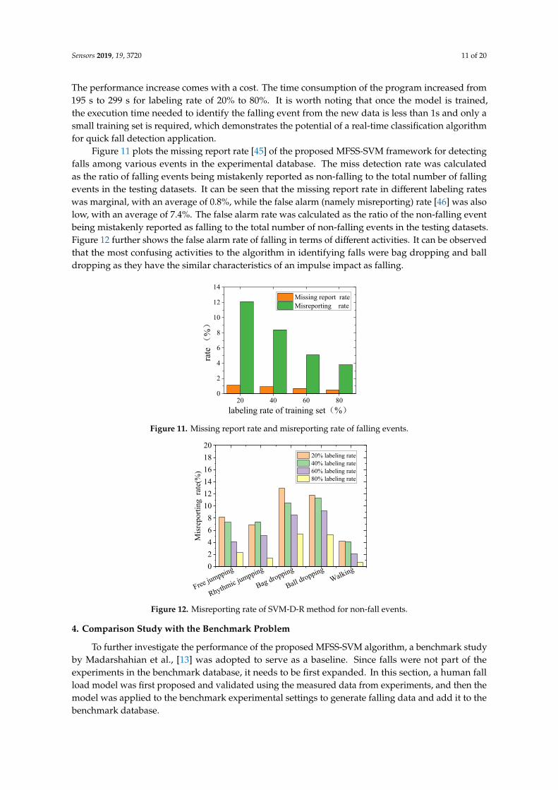
Figure 11 plots the missing report rate [45] of the proposed MFSS-SVM framework for detectingfalls among various events in the experimental database. The miss detection rate was calculatedas the ratio of falling events being mistakenly reported as non-falling to the total number of fallingevents in the testing datasets. It can be seen that the missing report rate in different labeling rateswas marginal, with an average of 0.8%, while the false alarm (namely misreporting) rate [46] was alsolow, with an average of 7.4%. The false alarm rate was calculated as the ratio of the non-falling eventbeing mistakenly reported as falling to the total number of non-falling events in the testing datasets.Figure 12 further shows the false alarm rate of falling in terms of different activities. It can be observedthat the most confusing activities to the algorithm in identifying falls were bag dropping and balldropping as they have the similar characteristics of an impulse impact as falling.


20 40 60 800

2

4

6

8

10

12

14

rate

（%）

labeling rate of training set（%）

Missing report rate Misreporting rate

Figure 11. Missing report rate and misreporting rate of falling events.

Figure 12. Misreporting rate of SVM-D-R method for non-fall events.

4. Comparison Study with the Benchmark Problem

To further investigate the performance of the proposed MFSS-SVM algorithm, a benchmark study by Madarshahian et al., [13] was adopted to serve as a baseline. Since falls were not part of the experiments in the benchmark database, it needs to be first expanded. In this section, a human fall load model was first proposed and validated using the measured data from experiments, and then the model was applied to the benchmark experimental settings to generate falling data and add it to the benchmark database.

4.1. Benchmark Problem

In the benchmark problem, human activity recognition was performed using acquired floor vibration signals. An algorithm based on an autocorrelation function was used to identify the events. In that study, floor vibrations caused by different activities, including plastic bag dropping, basketball ball dropping, and human jumping (shown in Table 6), were collected at a laboratory setting. The laboratory is located on the second floor of a two-story steel structure. Figure 13 shows the five excitation and four sensor locations.

Table 6. Data structure of benchmark database.

Event Type Event Amplitude Bag dropping Drop height 1.45 m/2.10 m Ball dropping Drop height 1.45 m/2.10 m Free jumping Weight 80 kg/55 kg/85 kg

Free jumpping

Rhythmic jumpping

Bag dropping

Ball droppingWalking0

2468

101214161820

Misr

epor

ting

rate

(%)

20% labeling rate 40% labeling rate 60% labeling rate 80% labeling rate



20 40 60 800

2

4

6

8

10

12

14

rate

（%）

labeling rate of training set（%）

Missing report rate Misreporting rate




To further investigate the performance of the proposed MFSS-SVM algorithm, a benchmark study by Madarshahian et al., [13] was adopted to serve as a baseline. Since falls were not part of the experiments in the benchmark database, it needs to be first expanded. In this section, a human fall load model was first proposed and validated using the measured data from experiments, and then the model was applied to the benchmark experimental settings to generate falling data and add it to the benchmark database.


In the benchmark problem, human activity recognition was performed using acquired floor vibration signals. An algorithm based on an autocorrelation function was used to identify the events. In that study, floor vibrations caused by different activities, including plastic bag dropping, basketball ball dropping, and human jumping (shown in Table 6), were collected at a laboratory setting. The laboratory is located on the second floor of a two-story steel structure. Figure 13 shows the five excitation and four sensor locations.


Event Type Event Amplitude Bag dropping Drop height 1.45 m/2.10 m Ball dropping Drop height 1.45 m/2.10 m Free jumping Weight 80 kg/55 kg/85 kg

Free jumpping

Rhythmic jumpping

Bag dropping

Ball droppingWalking0

2468

101214161820

Misr

epor

ting

rate

(%)

20% labeling rate 40% labeling rate 60% labeling rate 80% labeling rate



To further investigate the performance of the proposed MFSS-SVM algorithm, a benchmark studyby Madarshahian et al., [13] was adopted to serve as a baseline. Since falls were not part of theexperiments in the benchmark database, it needs to be first expanded. In this section, a human fallload model was first proposed and validated using the measured data from experiments, and then themodel was applied to the benchmark experimental settings to generate falling data and add it to thebenchmark database.

Sensors 2019, 19, 3720 12 of 20


In the benchmark problem, human activity recognition was performed using acquired floorvibration signals. An algorithm based on an autocorrelation function was used to identify theevents. In that study, floor vibrations caused by different activities, including plastic bag dropping,basketball ball dropping, and human jumping (shown in Table 6), were collected at a laboratory setting.The laboratory is located on the second floor of a two-story steel structure. Figure 13 shows the fiveexcitation and four sensor locations.


Event Type Event Amplitude

Bag dropping Drop height 1.45 m/2.10 mBall dropping Drop height 1.45 m/2.10 mFree jumping Weight 80 kg/55 kg/85 kg

Sensors 2019, 19, x; doi: FOR PEER REVIEW www.mdpi.com/journal/sensors

Article

Figure 13. Sensor and impact locations in benchmark experiment (unit: m) [12].

6.38

7.77

1.71

1.45

2.22

3.10

2.31

1.20

2.18

2.27

3.15

2.39

4.57

3.89

3.18

4.12

2.82

0.36

Sens

or 3

Loca

tion

2

Sens

or 1

Loca

tion

5

Sens

or 4

Loca

tion

4

Sens

or 2

Loca

tion

3

Loca

tion

1

Sens

orLo

catio

n


4.2. Human Fall Load Simulation

4.2.1. Fall Load Model

To expand the benchmark problem and add the falling datasets, a human falling model needsto be first defined. According to the state of consciousness during the process, human falling canbe divided into conscious and unconscious falls. Without completely losing consciousness, humanswill subconsciously use the knee, arm, and other parts of the body to land on the ground to reduceinjury. However, during unconscious falls, the person instantly collides with the ground withoutany protection, which would have a higher potential for severer injury. This study mainly focusedon unconscious backward fall caused by ground slipperiness, tripping, loss strength of leg muscles,and so on. In addition to its potential greater impact and thus larger significance and value of research,it was selected because the unconscious falling can be simulated by anthropomorphic dummies witheasier controllable experiment configurations. In the experimental study of a conscious fall involvingreal humans, sponge pads laying on the floor were often used to reduce the potential injury to thesubjects [47]. This not only increases the complexity by introducing additional dynamics but alsoweakens the vibration signal of the floor to a certain extent.

During the unconscious falling process, the external forces acting on the human body are gravityand the supporting force from the ground. The representative supporting force of an unconscious

Sensors 2019, 19, 3720 13 of 20

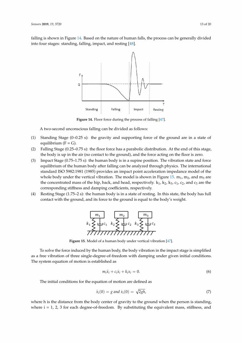
falling is shown in Figure 14. Based on the nature of human falls, the process can be generally dividedinto four stages: standing, falling, impact, and resting [48].



4.2. Human Fall Load Simulation

4.2.1. Fall Load Model

To expand the benchmark problem and add the falling datasets, a human falling model needs to be first defined. According to the state of consciousness during the process, human falling can be divided into conscious and unconscious falls. Without completely losing consciousness, humans will subconsciously use the knee, arm, and other parts of the body to land on the ground to reduce injury. However, during unconscious falls, the person instantly collides with the ground without any protection, which would have a higher potential for severer injury. This study mainly focused on unconscious backward fall caused by ground slipperiness, tripping, loss strength of leg muscles, and so on. In addition to its potential greater impact and thus larger significance and value of research, it was selected because the unconscious falling can be simulated by anthropomorphic dummies with easier controllable experiment configurations. In the experimental study of a conscious fall involving real humans, sponge pads laying on the floor were often used to reduce the potential injury to the subjects [46]. This not only increases the complexity by introducing additional dynamics but also weakens the vibration signal of the floor to a certain extent.

During the unconscious falling process, the external forces acting on the human body are gravity and the supporting force from the ground. The representative supporting force of an unconscious falling is shown in Figure 14. Based on the nature of human falls, the process can be generally divided into four stages: standing, falling, impact, and resting [47].

Figure 14. Floor force during the process of falling [46].

6.38

7.77

1.71

1.45

2.22

3.10

2.31

1.20

2.18

2.27

3.15

2.39

3.89

3.18

4.12

2.82

0.36Se

nsor 3

Locatio

n 2Se

nsor 1

Locatio

n 5

Senso

r 4Loc

ation 4

Senso

r 2

Locatio

n 3

Locatio

n 1

Figure 14. Floor force during the process of falling [47].

A two-second unconscious falling can be divided as follows:

(1) Standing Stage (0–0.25 s): the gravity and supporting force of the ground are in a state ofequilibrium (F = G).

(2) Falling Stage (0.25–0.75 s): the floor force has a parabolic distribution. At the end of this stage,the body is up in the air (no contact to the ground), and the force acting on the floor is zero.

(3) Impact Stage (0.75–1.75 s): the human body is in a supine position. The vibration state and forceequilibrium of the human body after falling can be analyzed through physics. The internationalstandard ISO 5982:1981 (1985) provides an impact point acceleration impedance model of thewhole body under the vertical vibration. The model is shown in Figure 15. m1, m2, and m3 arethe concentrated mass of the hip, back, and head, respectively. k1, k2, k3, c1, c2, and c3 are thecorresponding stiffness and damping coefficients, respectively.

(4) Resting Stage (1.75–2 s): the human body is in a state of resting. In this state, the body has fullcontact with the ground, and its force to the ground is equal to the body’s weight.



(1) Standing Stage (0–0.25 s): the gravity and supporting force of the ground are in a state of equilibrium (F = G).

(2) Falling Stage (0.25–0.75 s): the floor force has a parabolic distribution. At the end of this stage, the body is up in the air (no contact to the ground), and the force acting on the floor is zero.

(3) Impact Stage (0.75–1.75 s): the human body is in a supine position. The vibration state and force equilibrium of the human body after falling can be analyzed through physics. The international standard ISO 5982:1981 (1985) provides an impact point acceleration impedance model of the whole body under the vertical vibration. The model is shown in Figure 15. m1, m2, and m3 are the concentrated mass of the hip, back, and head, respectively. k1, k2, k3, c1, c2, and c3 are the corresponding stiffness and damping coefficients, respectively.

(4) Resting Stage (1.75–2 s): the human body is in a state of resting. In this state, the body has full contact with the ground, and its force to the ground is equal to the body’s weight.

Figure 15. Model of a human body under vertical vibration [46].

To solve the force induced by the human body, the body vibration in the impact stage is simplified as a free vibration of three single-degree-of-freedom with damping under given initial conditions. The system equation of motion is established as 𝑚 𝑥 + 𝑐 𝑥 + 𝑘 𝑥 = 0. (6)

The initial conditions for the equation of motion are defined as 𝑥 (0) = 𝑔 𝑎𝑛𝑑 𝑥 (0) = 2𝑔ℎ, (7)

where h is the distance from the body center of gravity to the ground when the person is standing, where i = 1,2,3 for each degree-of-freedom. By substituting the equivalent mass, stiffness, and damping parameters of the hip, back, and head into the model, the equation of motion can be used to solve for the acceleration. Then, according to equilibrium, the floor force F can be obtained as

𝐹 = 𝑚 𝑥 − 𝑚 𝑔. (8)

In 1981, the international standard organization established an impact point impedance, in which the data was collected from 12 volunteers weighted between 62.2 kg to 104 kg. The final model parameters were determined by averaging the acceleration impedance curves; a more detailed explanation can be found in document [46]. A typical floor force during the process of human falling (weight 71 kg) is shown in Figure 16.


To solve the force induced by the human body, the body vibration in the impact stage is simplifiedas a free vibration of three single-degree-of-freedom with damping under given initial conditions.The system equation of motion is established as

mi..xi + ci

.xi + kixi = 0. (6)

The initial conditions for the equation of motion are defined as

..xi(0) = g and

.xi(0) =

√2gh, (7)

where h is the distance from the body center of gravity to the ground when the person is standing,where i = 1, 2, 3 for each degree-of-freedom. By substituting the equivalent mass, stiffness, and

Sensors 2019, 19, 3720 14 of 20

damping parameters of the hip, back, and head into the model, the equation of motion can be used tosolve for the acceleration. Then, according to equilibrium, the floor force F can be obtained as

F =3∑

i=1

mi..xi −mig. (8)

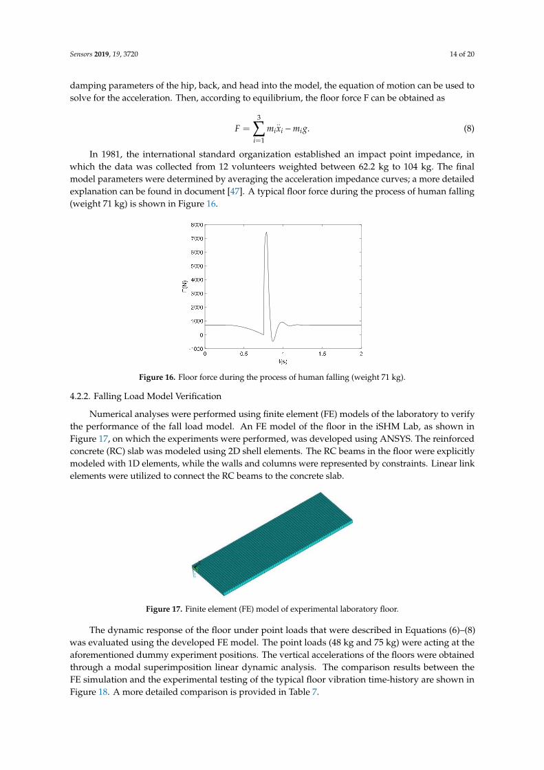
In 1981, the international standard organization established an impact point impedance, inwhich the data was collected from 12 volunteers weighted between 62.2 kg to 104 kg. The finalmodel parameters were determined by averaging the acceleration impedance curves; a more detailedexplanation can be found in document [47]. A typical floor force during the process of human falling(weight 71 kg) is shown in Figure 16.



(1) Standing Stage (0–0.25 s): the gravity and supporting force of the ground are in a state of equilibrium (F = G).

(2) Falling Stage (0.25–0.75 s): the floor force has a parabolic distribution. At the end of this stage, the body is up in the air (no contact to the ground), and the force acting on the floor is zero.

(3) Impact Stage (0.75–1.75 s): the human body is in a supine position. The vibration state and force equilibrium of the human body after falling can be analyzed through physics. The international standard ISO 5982:1981 (1985) provides an impact point acceleration impedance model of the whole body under the vertical vibration. The model is shown in Figure 15. m1, m2, and m3 are the concentrated mass of the hip, back, and head, respectively. k1, k2, k3, c1, c2, and c3 are the corresponding stiffness and damping coefficients, respectively.

(4) Resting Stage (1.75–2 s): the human body is in a state of resting. In this state, the body has full contact with the ground, and its force to the ground is equal to the body’s weight.


To solve the force induced by the human body, the body vibration in the impact stage is simplified as a free vibration of three single-degree-of-freedom with damping under given initial conditions. The system equation of motion is established as 𝑚 𝑥 + 𝑐 𝑥 + 𝑘 𝑥 = 0. (6)

The initial conditions for the equation of motion are defined as 𝑥 (0) = 𝑔 𝑎𝑛𝑑 𝑥 (0) = 2𝑔ℎ, (7)

where h is the distance from the body center of gravity to the ground when the person is standing, where i = 1,2,3 for each degree-of-freedom. By substituting the equivalent mass, stiffness, and damping parameters of the hip, back, and head into the model, the equation of motion can be used to solve for the acceleration. Then, according to equilibrium, the floor force F can be obtained as

𝐹 = 𝑚 𝑥 − 𝑚 𝑔. (8)

In 1981, the international standard organization established an impact point impedance, in which the data was collected from 12 volunteers weighted between 62.2 kg to 104 kg. The final model parameters were determined by averaging the acceleration impedance curves; a more detailed explanation can be found in document [46]. A typical floor force during the process of human falling (weight 71 kg) is shown in Figure 16.

Figure 16. Floor force during the process of human falling (weight 71 kg).

4.2.2. Falling Load Model Verification

Numerical analyses were performed using finite element (FE) models of the laboratory to verifythe performance of the fall load model. An FE model of the floor in the iSHM Lab, as shown inFigure 17, on which the experiments were performed, was developed using ANSYS. The reinforcedconcrete (RC) slab was modeled using 2D shell elements. The RC beams in the floor were explicitlymodeled with 1D elements, while the walls and columns were represented by constraints. Linear linkelements were utilized to connect the RC beams to the concrete slab.




Numerical analyses were performed using finite element (FE) models of the laboratory to verify the performance of the fall load model. An FE model of the floor in the iSHM Lab, as shown in Figure 17, on which the experiments were performed, was developed using ANSYS. The reinforced concrete (RC) slab was modeled using 2D shell elements. The RC beams in the floor were explicitly modeled with 1D elements, while the walls and columns were represented by constraints. Linear link elements were utilized to connect the RC beams to the concrete slab.

The dynamic response of the floor under point loads that were described in Equations (6)–(8) was evaluated using the developed FE model. The point loads (48 kg and 75 kg) were acting at the aforementioned dummy experiment positions. The vertical accelerations of the floors were obtained through a modal superimposition linear dynamic analysis. The comparison results between the FE simulation and the experimental testing of the typical floor vibration time-history are shown in Figure 18. A more detailed comparison is provided in Table 7.

Figure 17. Finite element (FE) model of experimental laboratory floor.

(a) Acceleration signal from sensor 4. 48 kg dummy

falling at position 2 (b) Acceleration signal from sensor 4. 75 kg dummy

falling at position 2

Figure 18. Comparison of simulated acceleration and experimental acceleration time history.

Table 7. Comparison of peak vertical acceleration from sensor 4 at position 2 (unit: g).

Experiment Dataset Simulation

Dummy Mean value Variance Median Minimum Maximum

48 kg 0.0334 1.2826e−4 0.0329 0.0152 0.0616 0.0643

75 kg 0.0382 8.5286e−5 0.0376 0.0196 0.0622 0.0597

As seen in Table 7, the FE simulations provided very similar vibrational performances and peak acceleration values as the experimental measurements. The falling process can be clearly divided into


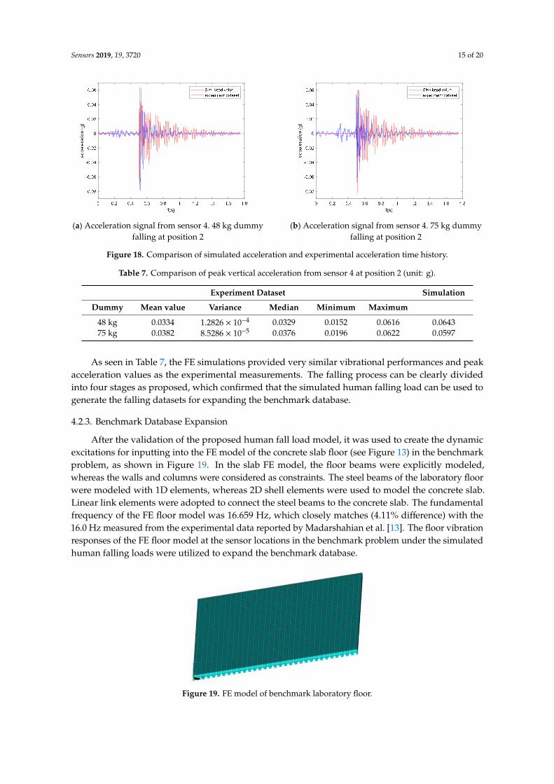
The dynamic response of the floor under point loads that were described in Equations (6)–(8)was evaluated using the developed FE model. The point loads (48 kg and 75 kg) were acting at theaforementioned dummy experiment positions. The vertical accelerations of the floors were obtainedthrough a modal superimposition linear dynamic analysis. The comparison results between theFE simulation and the experimental testing of the typical floor vibration time-history are shown inFigure 18. A more detailed comparison is provided in Table 7.

Sensors 2019, 19, 3720 15 of 20




Numerical analyses were performed using finite element (FE) models of the laboratory to verify the performance of the fall load model. An FE model of the floor in the iSHM Lab, as shown in Figure 17, on which the experiments were performed, was developed using ANSYS. The reinforced concrete (RC) slab was modeled using 2D shell elements. The RC beams in the floor were explicitly modeled with 1D elements, while the walls and columns were represented by constraints. Linear link elements were utilized to connect the RC beams to the concrete slab.

The dynamic response of the floor under point loads that were described in Equations (6)–(8) was evaluated using the developed FE model. The point loads (48 kg and 75 kg) were acting at the aforementioned dummy experiment positions. The vertical accelerations of the floors were obtained through a modal superimposition linear dynamic analysis. The comparison results between the FE simulation and the experimental testing of the typical floor vibration time-history are shown in Figure 18. A more detailed comparison is provided in Table 7.


(a) Acceleration signal from sensor 4. 48 kg dummy

falling at position 2 (b) Acceleration signal from sensor 4. 75 kg dummy

falling at position 2





48 kg 0.0334 1.2826e−4 0.0329 0.0152 0.0616 0.0643

75 kg 0.0382 8.5286e−5 0.0376 0.0196 0.0622 0.0597

As seen in Table 7, the FE simulations provided very similar vibrational performances and peak acceleration values as the experimental measurements. The falling process can be clearly divided into





48 kg 0.0334 1.2826 × 10−4 0.0329 0.0152 0.0616 0.064375 kg 0.0382 8.5286 × 10−5 0.0376 0.0196 0.0622 0.0597

As seen in Table 7, the FE simulations provided very similar vibrational performances and peakacceleration values as the experimental measurements. The falling process can be clearly dividedinto four stages as proposed, which confirmed that the simulated human falling load can be used togenerate the falling datasets for expanding the benchmark database.

4.2.3. Benchmark Database Expansion

After the validation of the proposed human fall load model, it was used to create the dynamicexcitations for inputting into the FE model of the concrete slab floor (see Figure 13) in the benchmarkproblem, as shown in Figure 19. In the slab FE model, the floor beams were explicitly modeled,whereas the walls and columns were considered as constraints. The steel beams of the laboratory floorwere modeled with 1D elements, whereas 2D shell elements were used to model the concrete slab.Linear link elements were adopted to connect the steel beams to the concrete slab. The fundamentalfrequency of the FE floor model was 16.659 Hz, which closely matches (4.11% difference) with the16.0 Hz measured from the experimental data reported by Madarshahian et al. [13]. The floor vibrationresponses of the FE floor model at the sensor locations in the benchmark problem under the simulatedhuman falling loads were utilized to expand the benchmark database.


four stages as proposed, which confirmed that the simulated human falling load can be used to generate the falling datasets for expanding the benchmark database.

4.2.3. Benchmark Database Expansion

After the validation of the proposed human fall load model, it was used to create the dynamic excitations for inputting into the FE model of the concrete slab floor (see Figure 13) in the benchmark problem, as shown in Figure 19. In the slab FE model, the floor beams were explicitly modeled, whereas the walls and columns were considered as constraints. The steel beams of the laboratory floor were modeled with 1D elements, whereas 2D shell elements were used to model the concrete slab. Linear link elements were adopted to connect the steel beams to the concrete slab. The fundamental frequency of the FE floor model was 16.659 Hz, which closely matches (4.11% difference) with the 16.0 Hz measured from the experimental data reported by Madarshahian et al. [13]. The floor vibration responses of the FE floor model at the sensor locations in the benchmark problem under the simulated human falling loads were utilized to expand the benchmark database.

Figure 19. FE model of benchmark laboratory floor.

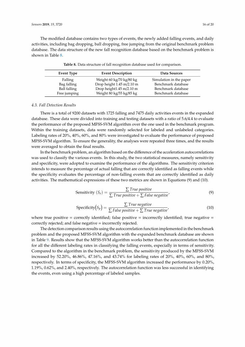
The modified database contains two types of events, the newly added falling events, and daily activities, including bag dropping, ball dropping, free jumping from the original benchmark problem database. The data structure of the new fall recognition database based on the benchmark problem is shown in Table 8.

Table 8. Data structure of fall recognition database used for comparison.

Event Type Event Description Data Sources

Falling Weight 60 kg/70 kg/80 kg Simulation in the paper

Bag falling Drop height 1.45 m/2.10 m Benchmark database

Ball falling Drop height1.45 m/2.10 m Benchmark database

Free jumping Weight 80 kg/55 kg/85 kg Benchmark database

4.3. Fall Detection Results

There is a total of 9200 datasets with 1725 falling and 7475 daily activities events in the expanded database. These data were divided into training and testing datasets with a ratio of 5.6/4.4 to evaluate the performance of the proposed MFSS-SVM algorithm over the one used in the benchmark program. Within the training datasets, data were randomly selected for labeled and unlabeled categories. Labeling rates of 20%, 40%, 60%, and 80% were investigated to evaluate the performance of proposed MFSS-SVM algorithm. To ensure the generality, the analyses were repeated three times, and the results were averaged to obtain the final results.

In the benchmark problem, an algorithm based on the difference of the acceleration autocorrelations was used to classify the various events. In this study, the two statistical measures, namely sensitivity and specificity, were adopted to examine the performance of the algorithms. The sensitivity criterion intends to measure the percentage of actual falling that are correctly identified as

Figure 19. FE model of benchmark laboratory floor.

Sensors 2019, 19, 3720 16 of 20

The modified database contains two types of events, the newly added falling events, and dailyactivities, including bag dropping, ball dropping, free jumping from the original benchmark problemdatabase. The data structure of the new fall recognition database based on the benchmark problem isshown in Table 8.

Table 8. Data structure of fall recognition database used for comparison.

Event Type Event Description Data Sources

Falling Weight 60 kg/70 kg/80 kg Simulation in the paperBag falling Drop height 1.45 m/2.10 m Benchmark databaseBall falling Drop height1.45 m/2.10 m Benchmark database

Free jumping Weight 80 kg/55 kg/85 kg Benchmark database

4.3. Fall Detection Results

There is a total of 9200 datasets with 1725 falling and 7475 daily activities events in the expandeddatabase. These data were divided into training and testing datasets with a ratio of 5.6/4.4 to evaluatethe performance of the proposed MFSS-SVM algorithm over the one used in the benchmark program.Within the training datasets, data were randomly selected for labeled and unlabeled categories.Labeling rates of 20%, 40%, 60%, and 80% were investigated to evaluate the performance of proposedMFSS-SVM algorithm. To ensure the generality, the analyses were repeated three times, and the resultswere averaged to obtain the final results.

In the benchmark problem, an algorithm based on the difference of the acceleration autocorrelationswas used to classify the various events. In this study, the two statistical measures, namely sensitivityand specificity, were adopted to examine the performance of the algorithms. The sensitivity criterionintends to measure the percentage of actual falling that are correctly identified as falling events whilethe specificity evaluates the percentage of non-falling events that are correctly identified as dailyactivities. The mathematical expressions of these two metrics are shown in Equations (9) and (10).

Sensitivity (Se) =

∑True positive∑

True positive +∑

False negative, (9)

Specificity(Sp

)=

∑True negative∑

False positive +∑

True negative, (10)

where true positive = correctly identified; false positive = incorrectly identified; true negative =

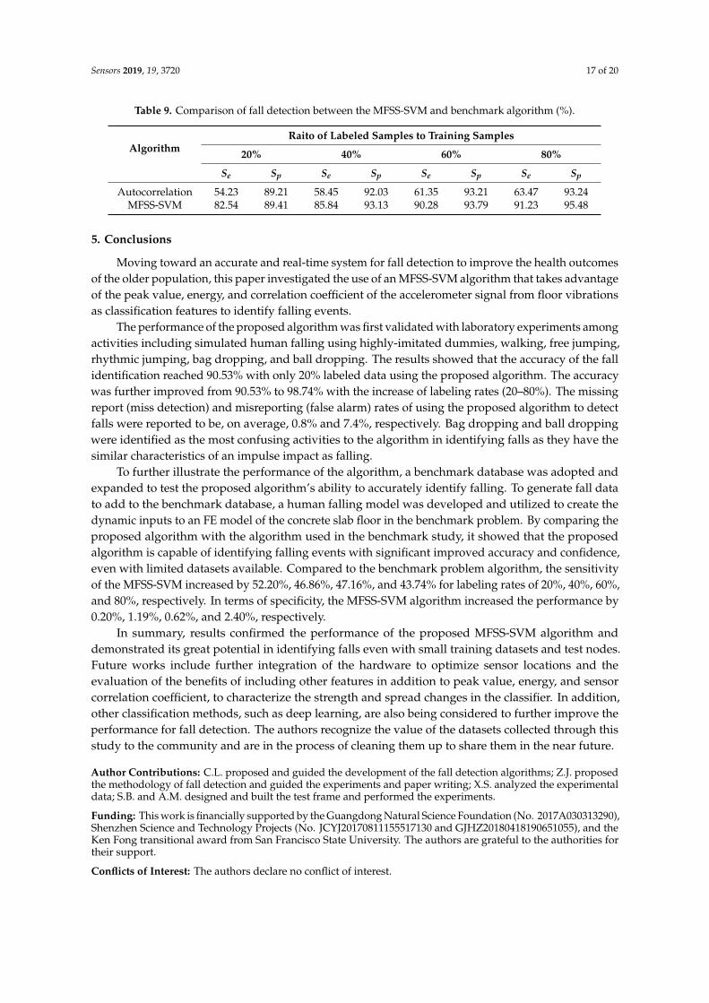
correctly rejected; and false negative = incorrectly rejected.The detection comparison results using the autocorrelation function implemented in the benchmark

problem and the proposed MFSS-SVM algorithm with the expanded benchmark database are shownin Table 9. Results show that the MFSS-SVM algorithm works better than the autocorrelation functionfor all the different labeling rates in classifying the falling events, especially in terms of sensitivity.Compared to the algorithm in the benchmark problem, the sensitivity produced by the MFSS-SVMincreased by 52.20%, 46.86%, 47.16%, and 43.74% for labeling rates of 20%, 40%, 60%, and 80%,respectively. In terms of specificity, the MFSS-SVM algorithm increased the performance by 0.20%,1.19%, 0.62%, and 2.40%, respectively. The autocorrelation function was less successful in identifyingthe events, even using a high percentage of labeled samples.

Sensors 2019, 19, 3720 17 of 20

Table 9. Comparison of fall detection between the MFSS-SVM and benchmark algorithm (%).

AlgorithmRaito of Labeled Samples to Training Samples

20% 40% 60% 80%

Se Sp Se Sp Se Sp Se Sp

Autocorrelation 54.23 89.21 58.45 92.03 61.35 93.21 63.47 93.24MFSS-SVM 82.54 89.41 85.84 93.13 90.28 93.79 91.23 95.48

5. Conclusions

Moving toward an accurate and real-time system for fall detection to improve the health outcomesof the older population, this paper investigated the use of an MFSS-SVM algorithm that takes advantageof the peak value, energy, and correlation coefficient of the accelerometer signal from floor vibrationsas classification features to identify falling events.

The performance of the proposed algorithm was first validated with laboratory experiments amongactivities including simulated human falling using highly-imitated dummies, walking, free jumping,rhythmic jumping, bag dropping, and ball dropping. The results showed that the accuracy of the fallidentification reached 90.53% with only 20% labeled data using the proposed algorithm. The accuracywas further improved from 90.53% to 98.74% with the increase of labeling rates (20–80%). The missingreport (miss detection) and misreporting (false alarm) rates of using the proposed algorithm to detectfalls were reported to be, on average, 0.8% and 7.4%, respectively. Bag dropping and ball droppingwere identified as the most confusing activities to the algorithm in identifying falls as they have thesimilar characteristics of an impulse impact as falling.

To further illustrate the performance of the algorithm, a benchmark database was adopted andexpanded to test the proposed algorithm’s ability to accurately identify falling. To generate fall datato add to the benchmark database, a human falling model was developed and utilized to create thedynamic inputs to an FE model of the concrete slab floor in the benchmark problem. By comparing theproposed algorithm with the algorithm used in the benchmark study, it showed that the proposedalgorithm is capable of identifying falling events with significant improved accuracy and confidence,even with limited datasets available. Compared to the benchmark problem algorithm, the sensitivityof the MFSS-SVM increased by 52.20%, 46.86%, 47.16%, and 43.74% for labeling rates of 20%, 40%, 60%,and 80%, respectively. In terms of specificity, the MFSS-SVM algorithm increased the performance by0.20%, 1.19%, 0.62%, and 2.40%, respectively.

In summary, results confirmed the performance of the proposed MFSS-SVM algorithm anddemonstrated its great potential in identifying falls even with small training datasets and test nodes.Future works include further integration of the hardware to optimize sensor locations and theevaluation of the benefits of including other features in addition to peak value, energy, and sensorcorrelation coefficient, to characterize the strength and spread changes in the classifier. In addition,other classification methods, such as deep learning, are also being considered to further improve theperformance for fall detection. The authors recognize the value of the datasets collected through thisstudy to the community and are in the process of cleaning them up to share them in the near future.

Author Contributions: C.L. proposed and guided the development of the fall detection algorithms; Z.J. proposedthe methodology of fall detection and guided the experiments and paper writing; X.S. analyzed the experimentaldata; S.B. and A.M. designed and built the test frame and performed the experiments.

Funding: This work is financially supported by the Guangdong Natural Science Foundation (No. 2017A030313290),Shenzhen Science and Technology Projects (No. JCYJ20170811155517130 and GJHZ20180418190651055), and theKen Fong transitional award from San Francisco State University. The authors are grateful to the authorities fortheir support.

Conflicts of Interest: The authors declare no conflict of interest.

Sensors 2019, 19, 3720 18 of 20

References

1. Roberts, A.W.; Ogunwole, S.U.; Blakeslee, L.; Rabe, M.A. The Population 65 Years and Older in the United States:2016; American Community Survey Reports; The United States Census Bureau: Suitland, MD, USA, 2018.

2. Centers for Disease Control and Prevention. The State of Aging and Health in AMERICA 2013; US Departmentof Health and Human Services, Centers for Disease Control and Prevention: Atlanta, GA, USA, 2013.

3. Centers for Disease Control and Prevention. Falls among Older Adults; Technical Report, September; USDepartment of Health and Human Services, Centers for Disease Control and Prevention: Atlanta, GA,USA, 2014.

4. Alert 1. Home Fall Detection Medical Alert. Available online: https://www.alert-1.com (accessed on 11April 2019).

5. Life Alert. Saving a Life from Potential Catastrophe Every 10 Minutes. Available online: http://www.lifealert.com/ (accessed on 11 April 2019).

6. GoLiveClip. Personal Safety in Every Situation. Available online: https://www.goliveclip.eu/solutions/goliveclip/ (accessed on 11 April 2019).

7. Mao, A.; Ma, X.; He, Y.; Luo, J. Highly Portable, Sensor-Based System for Human Fall Monitoring. Sensors2019, 17, 2096. [CrossRef] [PubMed]

8. Wu, Y.; Su, Y.; Feng, R.; Yu, N.; Zang, X. Wearable-sensor-based pre-impact fall detection system with ahierarchical classifier. Measurement 2019, 140, 283–292. [CrossRef]

9. Santos, G.; Endo, P.; Monteiro, K.; Rocha, E.; Silva, I.; Lynn, T. Accelerometer-Based Human Fall DetectionUsing Convolutional Neural Networks. Sensors 2019, 19, 1644. [CrossRef] [PubMed]

10. Belshaw, M.; Taati, B.; Snoek, J.; Mihailidis, A. Towards a single sensor passive solution for automated falldetection. In Proceedings of the Annual International Conference of the IEEE Engineering in Medicine andBiology Society, Boston, MA, USA, 30 August–3 September 2011; pp. 1773–1776.

11. Celik, O.; Dong, C.Z.; Catbas, F.N. A computer vision approach for the load time history estimation of livelyindividuals and crowds. Comput. Struct. 2018, 200, 32–52. [CrossRef]

12. Alwan, M.; Rajendran, P.J.; Kell, S.; Mack, D.; Dalal, S.; Wolfe, M.; Felder, R. A smart and passive floor-vibrationbased fall detector for elderly. In Proceedings of the Information and Communication Technologies, Lausanne,Switzerland, 24–28 April 2006; Volume 1, pp. 1003–1007.

13. Madarshahian, R.; Caicedo, J.M.; Zambrana, D.A. Benchmark problem for human activity identificationusing floor vibrations. Expert Syst. Appl. 2016, 62, 263–272. [CrossRef]

14. Poston, J.D.; Buehrer, R.M.; Tarazaga, P.A. Indoor footstep localization from structural dynamicsinstrumentation. Mech. Syst. Signal Process. 2017, 88, 224–239. [CrossRef]

15. Zigel, Y.; Litvak, D.; Gannot, I. A method for automatic fall detection of elderly people using floor vibrationsand sound—Proof of concept on human mimicking doll falls. IEEE Trans. Biomed. Eng. 2009, 56, 2858–2867.[CrossRef]

16. Davis, B.T. Characterization of Human-Induced Vibrations. Ph.D. Dissertation, University of South Carolina,Columbia, SC, USA, 2016. Available online: https://scholarcommons.sc.edu/etd/3770 (accessed on 25January 2019).

17. Dudani, S.A. The distance-weighted k-nearest-neighbor rule. IEEE Trans. Syst. Man Cybern. 1976, 4, 325–327.[CrossRef]

18. Weinberger, K.Q.; Saul, L.K. Distance metric learning for large margin nearest neighbor classification. J. Mach.Learn. Res. 2009, 10, 207–244.

19. Hearst, M.A.; Dumais, S.T.; Osuna, E.; Platt, J.; Scholkopf, B. Support vector machines. IEEE Intell. Syst. Appl.1998, 13, 18–28. [CrossRef]

20. Steinwart, I.; Christmann, A. Support Vector Machines; Springer Science & Business Media: Berlin/Heidelberg,Germany, 2008.

21. Zhang, H. The optimality of naive Bayes. AA 2004, 1, 3.22. Khan, A.M.; Lee, Y.K.; Lee, S.Y.; Kim, T.S. A triaxial accelerometer-based physical-activity recognition via

augmented-signal features and a hierarchical recognizer. IEEE Trans. Inf. Technol. Biomed. 2010, 14, 1166–1172.[CrossRef] [PubMed]

https://www.alert-1.com

http://www.lifealert.com/

http://www.lifealert.com/

https://www.goliveclip.eu/solutions/goliveclip/

https://www.goliveclip.eu/solutions/goliveclip/

http://dx.doi.org/10.3390/s17092096

http://www.ncbi.nlm.nih.gov/pubmed/28902149

http://dx.doi.org/10.1016/j.measurement.2019.04.002

http://dx.doi.org/10.3390/s19071644


http://dx.doi.org/10.1016/j.compstruc.2018.02.001

http://dx.doi.org/10.1016/j.eswa.2016.06.027

http://dx.doi.org/10.1016/j.ymssp.2016.11.023

http://dx.doi.org/10.1109/TBME.2009.2030171

https://scholarcommons.sc.edu/etd/3770

http://dx.doi.org/10.1109/TSMC.1976.5408784

http://dx.doi.org/10.1109/5254.708428

http://dx.doi.org/10.1109/TITB.2010.2051955


Sensors 2019, 19, 3720 19 of 20

23. Pirttikangas, S.; Fujinami, K.; Nakajima, T. Feature selection and activity recognition from wearable sensors.In International Symposium on Ubiquitious Computing Systems; Springer: Berlin/Heidelberg, Germany, 2006;pp. 516–527.

24. Cai, J.; Yang, K.Q.; Zhang, Y. Real-Time Physical Activity Recognition Using a Single Triaxial AccelerometerBased on HMM. In Applied Mechanics and Materials; Trans Tech Publications: Stafa-Zurich, Switzerland, 2014;Volume 602, pp. 2221–2224.

25. Boissy, P.; Choquette, S.; Hamel, M.; Noury, N. User-based motion sensing and fuzzy logic for automated falldetection in older adults. Telemed. e-Health 2007, 13, 683–694. [CrossRef] [PubMed]

26. Begg, R.; Kamruzzaman, J. A machine learning approach for automated recognition of movement patternsusing basic, kinetic and kinematic data. J. Biomech. 2005, 38, 401–408. [CrossRef] [PubMed]

27. Lau, H.Y.; Tong, K.Y.; Zhu, H. Support vector machine for classification of walking conditions using miniaturekinematic sensors. Med. Biol. Eng. Comput. 2008, 46, 563–573. [CrossRef]

28. Davis, B.T.; Caicedo, J.M.; Hirth, V.A.; Easterling, B.M. Acceleration Signal Categorization Using SupportVector Machines. Exp. Tech. 2019, 43, 359–368. [CrossRef]

29. Schölkopf, B.; Smola, A.J. Learning with Kernels. Support Vector Machines, Regularization, Optimization, andBeyond; MIT Press: Cambridge, MA, USA, 2002.

30. Vapnik, V.N. The Nature of Statistical Learning Theory; Springer: New York, NY, USA, 1995.31. Joachims, T. Transductive inference for text classification using support vector machines. In Proceedings of

the International Conference on Machine Learning, Bled, Slovenia, 27–30 July 1999; Volume 99, pp. 200–209.32. Bruzzone, L.; Chi, M.; Marconcini, M. A novel transductive SVM for semisupervised classification of

remote-sensing images. IEEE Trans. Geosci. Remote Sens. 2006, 44, 3363–3373. [CrossRef]33. Chen, Y.; Wang, G.; Dong, S. Learning with progressive transductive support vector machine. Pattern

Recognit. Lett. 2003, 24, 1845–1855. [CrossRef]34. Marconcini, M.; Camps-Valls, G.; Bruzzone, L. A composite semisupervised SVM for classification of

hyperspectral images. IEEE Geosci. Remote Sens. Lett. 2009, 6, 234–238. [CrossRef]35. Khan, S.S.; Hoey, J. Review of fall detection techniques: A data availability perspective. Med. Eng. Phys.

2017, 39, 12–22. [CrossRef]36. Liu, T.; Yao, H.; Ji, R.; Liu, Y.; Liu, X.; Sun, X.; Zhang, Z. Vision-based semi-supervised homecare with spatial

constraint. In Proceedings of the Pacific-Rim Conference on Multimedia, Tainan, Taiwan, 9–13 December2008; pp. 416–425.

37. Yang, K.; Ahn, C.R.; Vuran, M.C.; Aria, S.S. Semi-supervised near-miss fall detection for ironworkers with awearable inertial measurement unit. Autom. Constr. 2016, 68, 194–202. [CrossRef]

38. Blum, A.; Mitchell, T. Combining labeled and unlabeled data with co-training. In Proceedings of the EleventhAnnual Conference on Computational Learning Theory, Madison, WI, USA, 24–26 July 1998; pp. 92–100.

39. Zhou, Z.H.; Li, M. Tri-training: Exploiting unlabeled data using three classifiers. IEEE Trans. Knowl. Data Eng.2005, 17, 1529–1541. [CrossRef]

40. Mukhopadhyay, A.; Maulik, U.; Bandyopadhyay, S. Unsupervised cancer classification through SVM-boostedmultiobjective fuzzy clustering with majority voting ensemble. In Proceedings of the IEEE Congress onEvolutionary Computation, Trondheim, Norway, 18–21 May 2009; pp. 255–261.

41. Crammer, K.; Singer, Y. On the algorithmic implementation of multiclass kernel-based vector machines.J. Mach. Learn. Res. 2001, 2, 265–292.

42. Gangardiwala, A.; Polikar, R. Dynamically weighted majority voting for incremental learning and comparisonof three boosting based approaches. In Proceedings of the IEEE International Joint Conference on NeuralNetworks, Montreal, QC, Canada, 31 July–4 August 2005; Volume 2, pp. 1131–1136.

43. Deoliveira, M.J. Isotropic majority-vote model on a square lattice. J. Stat. Phys. 1992, 66, 273–281. [CrossRef]44. Krogh, A.; Vedelsby, J. Neural network ensembles, cross validation, and active learning. In Proceedings of the

Advances in Neural Information Processing Systems, Denver, CO, USA, 27–30 November 1995; pp. 231–238.45. Muhlenbach, F.; Lallich, S.; Zighed, D.A. Identifying and handling mislabelled instances. J. Intell. Inf. Syst.

2004, 22, 89–109. [CrossRef]46. Sun, J.W.; Zhao, F.Y.; Wang, C.J.; Chen, S.F. Identifying and correcting mislabeled training instances.

In Proceedings of the Future Generation Communication and Networking (FGCN 2007), Jeju, Korea, 6–8December 2007; Volume 1, pp. 244–250.

http://dx.doi.org/10.1089/tmj.2007.0007


http://dx.doi.org/10.1016/j.jbiomech.2004.05.002


http://dx.doi.org/10.1007/s11517-008-0327-x

http://dx.doi.org/10.1007/s40799-019-00318-y

http://dx.doi.org/10.1109/TGRS.2006.877950

http://dx.doi.org/10.1016/S0167-8655(03)00008-4

http://dx.doi.org/10.1109/LGRS.2008.2009324

http://dx.doi.org/10.1016/j.medengphy.2016.10.014

http://dx.doi.org/10.1016/j.autcon.2016.04.007

http://dx.doi.org/10.1109/TKDE.2005.186

http://dx.doi.org/10.1007/BF01060069

http://dx.doi.org/10.1023/A:1025832930864

Sensors 2019, 19, 3720 20 of 20

47. ISO 5982:1981. Vibration and Shock—Mechanical Driving Point Impedance of The Human Body. ISO 1985,5982, 1–5. Available online: https://www.iso.org/standard/12174.html (accessed on 11 April 2019).

48. Casilari, E.; Santoyo-Ramón, J.A.; Cano-García, J.M. UMAFall: A Multisensor Dataset for the Research onAutomatic Fall Detection. Procedia Comput. Sci. 2017, 110, 32–39. [CrossRef]

© 2019 by the authors. Licensee MDPI, Basel, Switzerland. This article is an open accessarticle distributed under the terms and conditions of the Creative Commons Attribution(CC BY) license (http://creativecommons.org/licenses/by/4.0/).

https://www.iso.org/standard/12174.html

http://dx.doi.org/10.1016/j.procs.2017.06.110

http://creativecommons.org/

http://creativecommons.org/licenses/by/4.0/.

Documents

Detection of Human Fall Using Floor Vibration and Multi