Embed Size (px)
Citation preview

DETECTION OF FEMUR FRACTURES IN X-RAYIMAGES
TIAN TAI PENG
NATIONAL UNIVERSITY OF SINGAPORE2002

Name : Tian Tai PengDegree : Master of ScienceDept : Computer ScienceThesis Title : Detection of Femur Fractures in X-Ray Images
Abstract
Many people suffer from hip fractures, especially people suffering from os-teoporosis. Doctors rely on radiographs, i.e., x-ray images, to establish theprecise nature of a fracture. An automated fracture detection system canassist the doctor by performing the first examination to screen out the easiercases, leaving a small number of difficult cases and the second confirmationto the doctors. This thesis outlines a fracture detection system and focuson measuring the neck-shaft angle of the femur. The accuracy of using theneck-shaft angle for determining femur fractures is also tested.
Keywords:
Neck-shaft angle, femur fractures, active contour
DETECTION OF FEMUR FRACTURES IN
X-RAY IMAGES
Tian Tai Peng(B. Sc. (Hon.) in Computer and Information Sciences, NUS)
A THESIS SUBMITTEDFOR THE DEGREE OF MASTER OF SCIENCE
DEPARTMENT OF COMPUTER SCIENCESCHOOL OF COMPUTING
NATIONAL UNIVERSITY OF SINGAPORE2002

Contents
1 Introduction 3
1.1 Motivation . . . . . . . . . . . . . . . . . . . . . . . . . . . . . 31.2 The Femur . . . . . . . . . . . . . . . . . . . . . . . . . . . . . 61.3 Anatomy of Fracture . . . . . . . . . . . . . . . . . . . . . . . 101.4 Project Objectives . . . . . . . . . . . . . . . . . . . . . . . . 131.5 Organization of Thesis . . . . . . . . . . . . . . . . . . . . . . 15
2 Related Work 16
2.1 Free-Form Deformable Model . . . . . . . . . . . . . . . . . . 172.1.1 Centroid-Radii Model . . . . . . . . . . . . . . . . . . . 182.1.2 Curvature Primal Sketch . . . . . . . . . . . . . . . . . 18
2.2 Parametric Deformable Templates . . . . . . . . . . . . . . . . 192.3 Point Distribution Model . . . . . . . . . . . . . . . . . . . . . 202.4 Graphical Template Model . . . . . . . . . . . . . . . . . . . . 212.5 Skeleton Based Model . . . . . . . . . . . . . . . . . . . . . . 22
3 Extraction of Femur Contour 24
3.1 Modified Canny Edge Detection . . . . . . . . . . . . . . . . . 253.2 Snakes and Active Contours . . . . . . . . . . . . . . . . . . . 283.3 Gradient Vector Flow . . . . . . . . . . . . . . . . . . . . . . . 323.4 Combining Snake with GVF . . . . . . . . . . . . . . . . . . . 33
4 Measuring Neck-Shaft Angle from Femur Contour 35
4.1 Computing Level Lines . . . . . . . . . . . . . . . . . . . . . . 364.2 Computing Orientation of the Femoral Shaft . . . . . . . . . . 384.3 Computing the Orientation of the Femoral Neck . . . . . . . . 38
4.3.1 Computing Initial Estimation of Femoral Neck’s Ori-entation . . . . . . . . . . . . . . . . . . . . . . . . . . 40
4.3.2 Smoothing the Original Contour . . . . . . . . . . . . . 424.3.3 Computing the Axis of Symmetry for the Femoral Head
and Neck . . . . . . . . . . . . . . . . . . . . . . . . . 43

Contents
5 Test Results and Discussion 46
5.1 Classification using Neck-Shaft Angle . . . . . . . . . . . . . . 465.1.1 Test Setup . . . . . . . . . . . . . . . . . . . . . . . . . 465.1.2 Test Results . . . . . . . . . . . . . . . . . . . . . . . . 475.1.3 Discussion on Classification Results . . . . . . . . . . . 52
6 Future Work 56
7 Conclusion 59
Bibliography 61
ii

List of Figures
1.1 Comparison between osteoporotic and healthy bone. . . . . . . 41.2 Common fracture sites for osteoporosis . . . . . . . . . . . . . 41.3 A radiograph example of the hip. . . . . . . . . . . . . . . . . 61.4 Anterior skeleton anatomy . . . . . . . . . . . . . . . . . . . . 71.5 Upper extremity and body of the femur. . . . . . . . . . . . . 91.6 Lower extremity of the femur. . . . . . . . . . . . . . . . . . . 91.7 Neck-shaft angle . . . . . . . . . . . . . . . . . . . . . . . . . . 101.8 Femoral neck fracture. . . . . . . . . . . . . . . . . . . . . . . 111.9 Intertrochanteric fracture. . . . . . . . . . . . . . . . . . . . . 121.10 Greater trochanteric fracture. . . . . . . . . . . . . . . . . . . 121.11 Subtrochanteric fracture. . . . . . . . . . . . . . . . . . . . . . 131.12 Project Overview. . . . . . . . . . . . . . . . . . . . . . . . . . 14
2.1 Medial Axis . . . . . . . . . . . . . . . . . . . . . . . . . . . . 22
3.1 Femur contour extraction algorithm. . . . . . . . . . . . . . . 253.2 Difficulty in detecting femur head edges. . . . . . . . . . . . . 263.3 Different threshold for modified Canny edge detector. . . . . . 283.4 Snake in action. . . . . . . . . . . . . . . . . . . . . . . . . . . 34
4.1 Normal lines on the femur shaft. . . . . . . . . . . . . . . . . . 364.2 Midpoints of Level Lines . . . . . . . . . . . . . . . . . . . . . 394.3 Level Lines . . . . . . . . . . . . . . . . . . . . . . . . . . . . 414.4 Smoothing the femur contour. . . . . . . . . . . . . . . . . . . 434.5 Generating a prospective line. . . . . . . . . . . . . . . . . . . 454.6 Contour points and its reflection. . . . . . . . . . . . . . . . . 45
5.1 Neck-shaft angle measurement for left femurs. . . . . . . . . . 485.2 Neck-shaft angle measurement for right femurs. . . . . . . . . 495.3 Difference betweeen left and right femurs. . . . . . . . . . . . . 505.4 Femurs correctly classified as healthy . . . . . . . . . . . . . . 535.5 Femurs correctly classified as fractured . . . . . . . . . . . . . 53

List of Figures
5.6 Misclassification as healthy . . . . . . . . . . . . . . . . . . . . 545.7 Misclassification as fracture . . . . . . . . . . . . . . . . . . . 55
6.1 Trabecular lines. . . . . . . . . . . . . . . . . . . . . . . . . . 57
iv

List of Tables
5.1 Summary of classification results. . . . . . . . . . . . . . . . . 51

List of Algorithms
1 Computing initial estimation of femoral neck’s orientation. . . 42

Summary
Many people suffer from hip fractures, especially people suffering from os-
teoporosis. Doctors rely on radiographs, i.e., x-ray images, to establish the
precise nature of a fracture. An automated fracture detection system can
assist the doctor by performing the first examination to screen out the easier
cases, leaving a small number of difficult cases and the second confirmation
to the doctors.
This thesis outlines a fracture detection system, and focuses on the ex-
traction of the femur bone contour and measurement of the femoral neck-
shaft angle. Snakes combine with Gradient Vector Flow field are used to
extract the femur outline. Given the boundary contour, the orientations of
the femoral shaft and the femoral neck are computed. The angle between
these two orientations is the neck-shaft angle. Using the neck-shaft angle
as a criterion for discriminating between fractured and healthy femurs, the
method achieves a correct classification rate of 94.5%.

Chapter 1
Introduction
1.1 Motivation
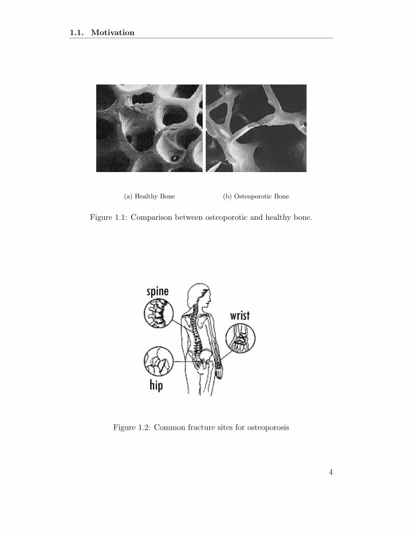
Many people suffer from fractures of the bone, especially people suffering
from osteoporosis. Osteoporosis is a disease characterized by low bone mass
and deterioration of bone tissue (Fig 1.1). This condition leads to increased
bone fragility and risk of fracture. If not prevent or left untreated, the
disease can progress painlessly until a bone breaks. Osteoporosis related
bone fractures occur typically in the hip, spine and wrist (Fig 1.2). Any
bone can be affected but of special concern are fractures of the hip as such
fractures almost always requires hospitalization and major surgery. It can
also impair a person’s ability to walk unassisted and may cause prolonged or
permanent disability.
Some 800 people suffer hip fractures in Singapore every year due to os-
teoporosis and Singapore General Hospital (SGH) sees about 350 of such
1.1. Motivation
(a) Healthy Bone (b) Osteoporotic Bone
Figure 1.1: Comparison between osteoporotic and healthy bone.
Figure 1.2: Common fracture sites for osteoporosis
4

1.1. Motivation
patients each year. According to studies, a quarter of the hip fractured pa-
tients die within the first year and seventy percent of the survivors require
walking aids, became wheelchair bound or bedridden [33].
Doctors rely on radiographs, i.e., x-ray images, to establish the precise
nature of a fracture (see Fig 1.3). Currently doctors in Singapore General
Hospital examine each radiograph twice to determine whether a fracture
exists. Manual inspection of radiographs for fractures is both a tedious and
time consuming process. On top of that, doctors will get too tired to perform
the task reliably after examining numerous radiographs. As some fractures
are easier to identify than others, an automated fracture detection system can
assist the doctor by performing the first examination to screen out the easier
cases, leaving a small number of difficult cases and the second confirmation
to the doctors. Automatic interpretation of medical images can relieve some
of the labor intensive work of the doctors thus improving the accuracy of the
diagnosis.
In this research, emphasis will be placed on detecting common hip frac-
tures of the femur as such fractures account for the largest portion of fracture
incidents in the population. Section 1.2 will explain in detail the anatomy of
the femur and Section 1.3 will describe different fractures of the femur.
5

1.2. The Femur
Figure 1.3: A radiograph example of the hip.
1.2 The Femur
The femur is the longest and strongest bone in the skeleton. It is connected
to the pelvis to form the hip joint and connected to the tibia to form the
upper knee joint (Fig. 1.4). Each femur directly bears the weight of the upper
body.
The femur is almost perfectly cylindrical in the greater part of its ex-
tent. It is divisible into a body and two extremities: the upper and lower
extremities.
The Body or Shaft
The body or shaft, almost cylindrical in form, is a little broader above
than in the center (Fig 1.5). It is slightly arched, so as to be convex in
6

1.2. The Femur
Figure 1.4: Anterior skeleton anatomy
7

1.2. The Femur
front and concave behind.
Upper Extremity
The upper extremity comprises the head, neck, a greater trochanter
and a lesser trochanter (Fig. 1.5). The head is globular and the neck is
a flattened pyramidal bone connecting the head with the shaft of the
femur. The neck forms an angle of about 125 degrees with the shaft,
but it varies in inverse proportion to the development of the pelvis.
The angle also varies considerably in different persons of the same age.
The greater and lesser trochanters provide leverage to the muscles that
rotate the thighs on it axes.
Lower Extremity
The lower extremity is somewhat cuboid in form and it consists of two
oblong eminences known as the condyle (Fig 1.6)
Neck-Shaft Angle
The neck-shaft angle is commonly used by doctors to detect fractures in
the femur. The neck-shaft angle is determined by measuring the angle
subtended by the lines drawn through the axes of the femoral shaft and
the femoral neck (Fig 1.7). The neck-shaft angle for a healthy adult
femur is approximately 120 to 130 degrees.
8

1.2. The Femur
Figure 1.5: Upper extremity and body of the femur.
Figure 1.6: Lower extremity of the femur.
9

1.3. Anatomy of Fracture
Figure 1.7: Neck-shaft angle
1.3 Anatomy of Fracture
A fracture may be a complete break in the continuity of a bone or it may be
an incomplete break or crack. The fracture site is often used to classify the
type fracture. Hip fractures can be classified as head, neck, intertrochanteric,
trochanteric or subtrochanteric. The following is a classification found in [16].
Femoral Neck Fractures
Femoral neck fractures occur between the end of the femoral head and
the intertrochanteric region (Fig 1.8).
Intertrochanteric Fractures
10

1.3. Anatomy of Fracture
(a) (b)
Figure 1.8: Femoral neck fracture (b) occurs at the femoral neck region (a).
Intertrochanteric fractures occur in the bone between the femoral neck
and the femoral shaft (Fig 1.9). These fractures may involve both the
greater and lesser trochanter.
Greater Trochanteric Fractures
This type of fracture occurs in the greater trochanter (Fig 1.10). It
may occur in elderly patients suffering from osteoporosis and may result
from direct trauma such as a fall.
Subtrochanteric Fractures
Subtrochanteric fractures occur between the lesser trochanter and the
shaft of the femur (Fig 1.11).
11

1.3. Anatomy of Fracture
(a) (b)
Figure 1.9: Intertrochanteric fracture (b) occurs at the intertrochanteric re-gion (a).
(a) (b)
Figure 1.10: Greater trochanteric fracture (b) occurs at the greatertrochanteric region (a).
12

1.4. Project Objectives
(a) (b)
Figure 1.11: Subtrochanteric fracture (b) occurs at the subtrochanteric region(a).
1.4 Project Objectives
The overall goal of the project is to develop a system to detect fractures of
the femur automatically, which consists of three modules (Figure 1.12).
Firstly, given an x-ray image of the hip, the Femur Localization module
will need to find the location of the left and right femur in the image. Precise
object localization is a difficult problem in computer vision. This module is
investigated by another student and is thus not the focus of this thesis.
Next, to analyze the geometry of the femur, a more accurate outline of the
femur is needed. The locations of the two femurs identified by the “Femur
Localization” module will serve as the initial search locations in the “Femur
Contour Extraction module”. Active contours, also know as snakes [23] are
used in the “Femur Contour Extraction” module. If a snake is placed close
13
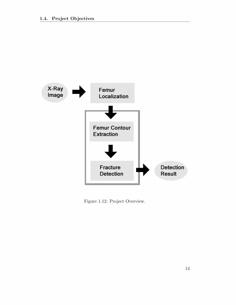
1.4. Project Objectives
Figure 1.12: Project Overview.
14

1.5. Organization of Thesis
to the femur outline, the snake algorithm will make use of image features
to guide and deform itself to converge on the outline of the femur. The
output from the snake algorithm is a more accurate description of the femur’s
boundary contour and is more suitable for analyzing potential fracture of the
femur.
Finally, in the “Fracture Detection” module, the contour of the femurs
will be analyzed to compute the neck-shaft angles. Any femurs with abnormal
neck-shaft angles will be classified as fractured.
In summary, the main objective of this thesis is to develop the algo-
rithms necessary for the “Femur Contour Extraction” and “Fracture Detec-
tion” modules.
1.5 Organization of Thesis
After highlighting the motivation and project objectives in this chapter, re-
lated work will be reviewed in Chapter 2. The details of the algorithms for
the “Femur Contour Extraction” and “Fracture Detection” module will be
discussed in Chapter 3 and Chapter 4 respectively. Experimental results of
the algorithms are discussed in Chapter 5. Finally, future direction for this
work is highlighted in Chapter 6, followed by the conclusion in Chapter 7.
15

Chapter 2
Related Work
Medical image interpretation is a hard problem as any non-trivial algorithm
will involve some form of automated system to understand the information
contained in the image. Fortunately, the general shape, location and orien-
tation of the objects of interest are usually known in medical image analysis.
Such information may be represented in a model of the object as initial con-
ditions, constraints on model parameters or constraints during model fitting
procedure. Once the model has been established, analysis of the model can
take place.
There is a wealth of model representations used in medical image interpre-
tation literature. They include free-form deformable models [23, 31, 32], para-
metric deformable templates [36], point distribution model [11, 12], graphical
templates [3] and skeleton-based templates [29, 30].

2.1. Free-Form Deformable Model
2.1 Free-Form Deformable Model
Free-form deformable models contains no global structure except for some
regularization constraints such as continuity or smoothness constraint of the
boundary. Without any constraints on the global shape, it can represent
arbitrary shape as long as it satisfies the regularization constraints.
Active contours [23, 31, 32] or snakes are good examples of free-form
deformable models. These contours will evolve under the influence of image
forces (such a edges or intensity) that pull it towards desired features and
internal forces that enforce smoothness and continuity constraints on the
contour.
This approach of evolving based on local image features makes the snake
more vulnerable to image noise and initial position. Many improvements
have been suggested to overcome these shortcomings [1, 9, 10, 34].
With an initialization that places the snake close to the object boundaries,
the snake algorithm can extract an accurate representation of the object’s
outline. Such detailed outlines are useful for constructing higher level repre-
sentation of the contour such as centroid-radii model [8, 20] and the curvature
primal sketch [4, 26].
17

2.1.1 Centroid-Radii Model
2.1.1 Centroid-Radii Model
The centroid-radii model [8, 20] samples a set of points from the outline of
the object. These points will be used to re-parameterize the original contour
in terms of the distance from the centroid to the points (call radii lines) as
well as the angle from a reference line to the radii lines.
This approach is useful for objects with fairly consistent shape but in the
case of femur fractures, the centroid may be drastically different from one
case to the other.
2.1.2 Curvature Primal Sketch
Curvature primal sketch [4] extracts significant changes in curvature along the
contour across varying levels of details (i.e., multiple level of curve smoothing)
called the generalized scale space image of planar curve [26]. These changes
are classified into five different groups of primitives based on the curvature
discontinuity and are used for matching purposes.
This technique has been successfully used for object recognition [27] but
the representation is too sparse for fracture detection. For example in some
fracture incidents, it may not increase or decrease the number of curvature
primal sketch primitives. Hence, this will pose a problem when trying to
detect fractures based on such primitives. Furthermore, the lesser trochanter
18
2.2. Parametric Deformable Templates
may not be present in all the femur images and may thus flag off a wrong
alert during fracture detection.
2.2 Parametric Deformable Templates
Deformable templates [36] are hand-crafted models represented by a collec-
tion of parameterized curves. These curves are uniquely described by a set
of parameters. Changing the parameters will change the geometric shape of
the template.
A good example is the work of Yuille et al. [36] who constructed de-
formable templates to extract facial features. Their parametric models for
eye and mouth templates consist of circles and parabolic curves. The shape
of the template is controlled by the radius of the circle and the parameters
of the parabola. A set of regularizing constraints are used to impose on
the shape to limit the deformations such that it result in reasonable shapes.
By defining energy terms describing the deformation of the template and
energy terms for the image features, the detection algorithm will become a
minimization procedure based on the energy terms.
For this technique a good initialization of the contour is necessary for good
results. On top of that, this scheme is not suitable for shapes with compli-
cated outlines as it will be difficult to describe the outline using a small set
19

2.3. Point Distribution Model
of curves. Secondly the approximate orientation, scale and translation of the
object to be segmented has to be known beforehand to craft the regularizing
constraints and it will be difficult to build a template encompassing all the
different classes of fractures.
2.3 Point Distribution Model
The Point Distribution Models (PDM) [14, 25] approach assumes the exis-
tence of a set of training examples from which to derive a statistical descrip-
tion of the shape and its variation. This approach is most useful for describing
objects that have well understood general shape but which cannot be easily
described by a rigid model.
The shape is defined as all the geometrical information that remains when
location, scale and rotational effects are filtered out from an object [15].
One way to represent a shape is to locate a finite number of points on the
boundary of the object (a sequence of pixel co-ordinates) called landmark
points. To ensure that the set of points satisfy the definition of a shape,
the effects of scale, translation and rotation are filtered out by aligning the
training samples. A common procedure for aligning the data is the Procrustes
Analysis [6, 13, 18]. Principal Component Analysis space is used to extract a
parameterized model of the training data and with this parameterized model,
20

2.4. Graphical Template Model
it allows new shapes, different from the training samples, to be synthesized.
Point distribution models are used in Active Shape Models [11, 12, 13]
to search for objects of interest in an image using the PDM. The search is
formulated as an optimization problem in which the difference between the
synthesized shape and the actual image is to be minimized. This algorithm
has been proven to be successful in medical segmentation [5] and analysis [19].
The main drawback of this approach is that the PDM requires human
intervention to annotate landmark points in the training images and this can
be very time consuming. Currently automatic and semi-automatic methods
are being developed to aid this task of annotating landmark points.
2.4 Graphical Template Model
The model in a Graphical Template [2, 3] is represented as a graph. Vertices
will represent landmark points and edges represent important geometric re-
lations among the landmark points. Such graphs are usually hand-crafted
and differ from application to application.
The Graphical Template Model is used mainly as a registration algorithm.
The algorithm attempts to localize the model by scanning for candidates of
each of the landmarks. These landmarks are extracted from the image using
robust local operators. The collection of landmark points which satisfy the
21
2.5. Skeleton Based Model
graph constraints and yielding the best match, will be chosen to represent
the object in the image.
2.5 Skeleton Based Model
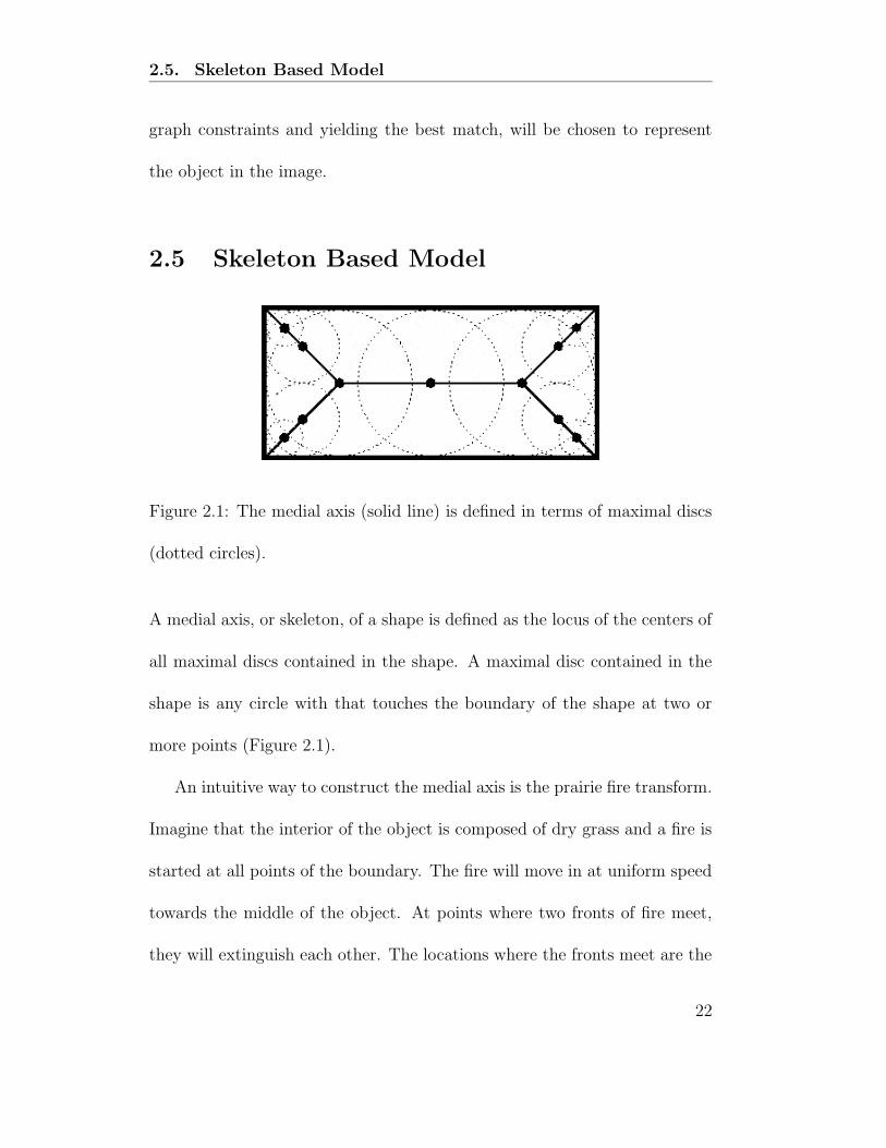
Figure 2.1: The medial axis (solid line) is defined in terms of maximal discs
(dotted circles).
A medial axis, or skeleton, of a shape is defined as the locus of the centers of
all maximal discs contained in the shape. A maximal disc contained in the
shape is any circle with that touches the boundary of the shape at two or
more points (Figure 2.1).
An intuitive way to construct the medial axis is the prairie fire transform.
Imagine that the interior of the object is composed of dry grass and a fire is
started at all points of the boundary. The fire will move in at uniform speed
towards the middle of the object. At points where two fronts of fire meet,
they will extinguish each other. The locations where the fronts meet are the
22
2.5. Skeleton Based Model
locations of the medial axis points.
Shape modeling typically requires a robust variant of the traditional me-
dial axis so that small changes in the outline of the shape does not severely
alter its topology [17]. Most skeleton extraction algorithms require a seg-
mented image as the input. An exception is the algorithm proposed by Pizer
et al. [30] where they introduced a model comprising of nets of medial and
boundary primitives. This model can estimate the boundary of the object
and its medial axis based on the intensity gradient in the original gray scale
image.
23

Chapter 3
Extraction of Femur Contour
An overview of the algorithm for extracting the contour of the femur is shown
in Figure 3.1. It consists of a sequence of processes. First a modified Canny
edge detector (Section 3.1) is used to compute the edges from the input x-ray
image of the hip followed by computing the Gradient Vector Flow field [34]
(Section 3.3) for the edges. Next, the snake algorithm [23] (Section 3.2)
combine with the Gradient Vector Flow will move the active contour, i.e, the
snake to the contour of the femur.
For the snake algorithm to work well, the initial points of the snake should
be placed close to the femur boundary. Currently the initial points of the
snake are placed manually as automatic placement of the initial points of the
snake is a difficult problem and it is not the focus of this thesis.

3.1. Modified Canny Edge Detection
Figure 3.1: Femur contour extraction algorithm.
3.1 Modified Canny Edge Detection
The Canny edge detector [7] takes as input a gray scale image and produces
as output an image showing the position of the edges. It works as follows.
The image is first smoothed by Gaussian convolution. Next, a simple 2D first
derivative operator is applied to the smoothed image to highlight regions of
the image with high first derivatives. Using the gradient direction calculated,
the algorithm performs non-maxima suppression to eliminate pixels whose
gradient magnitude is lower than its two neighbors along the gradient di-
rection. Finally these thin edges are linked up using a technique involving
double thresholding. Although Canny edge detector works well in detecting
the outline of the femur, it also detects a large number of spurious edges
close to the shaft (Figure 3.2b). Such spurious edges will affect the snake’s
25
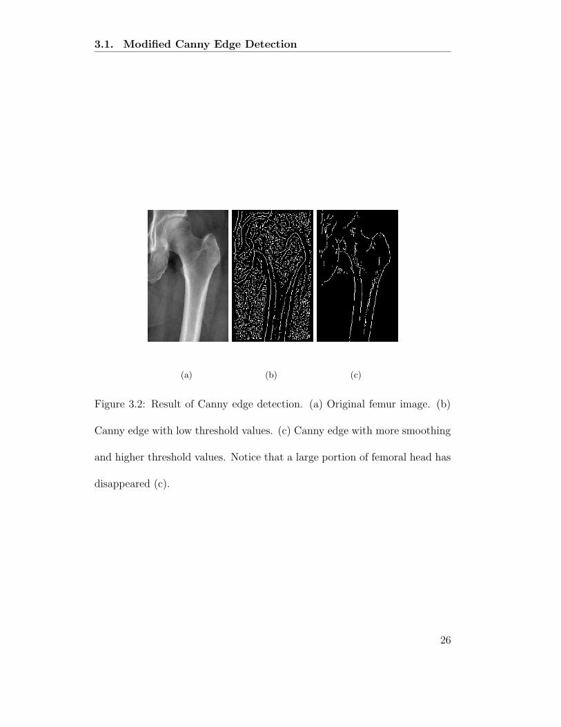
3.1. Modified Canny Edge Detection
(a) (b) (c)
Figure 3.2: Result of Canny edge detection. (a) Original femur image. (b)
Canny edge with low threshold values. (c) Canny edge with more smoothing
and higher threshold values. Notice that a large portion of femoral head has
disappeared (c).
26

3.1. Modified Canny Edge Detection
convergence on the outline of the femur and have to be removed. Attempting
to remove the spurious edges by increasing the smoothing effect will reduce
these spurious edges but the edge information at the femur head will also be
lost (Figure 3.2c). Contributing to the problem is the fact that the femur
head overlaps with the hip bones and edge magnitudes of the femur head in
this region is low. Hence simple thresholding based on edge magnitude will
fail .
The problem of preserving femur head edges and at the same time re-
moving spurious edges can be solved by incorporating information from the
intensity image into the Canny edge algorithm. Looking at the original in-
tensity x-ray image of the femur (Figure 3.2a), areas containing bones have
higher intensity than non-bone regions. Hence this information can be used
to distinguish spurious edges from femur head edges. The Canny edge de-
tector with a small smoothing effect is used to detect the femur head edges
while spurious edges with both low intensity value and low gradient magni-
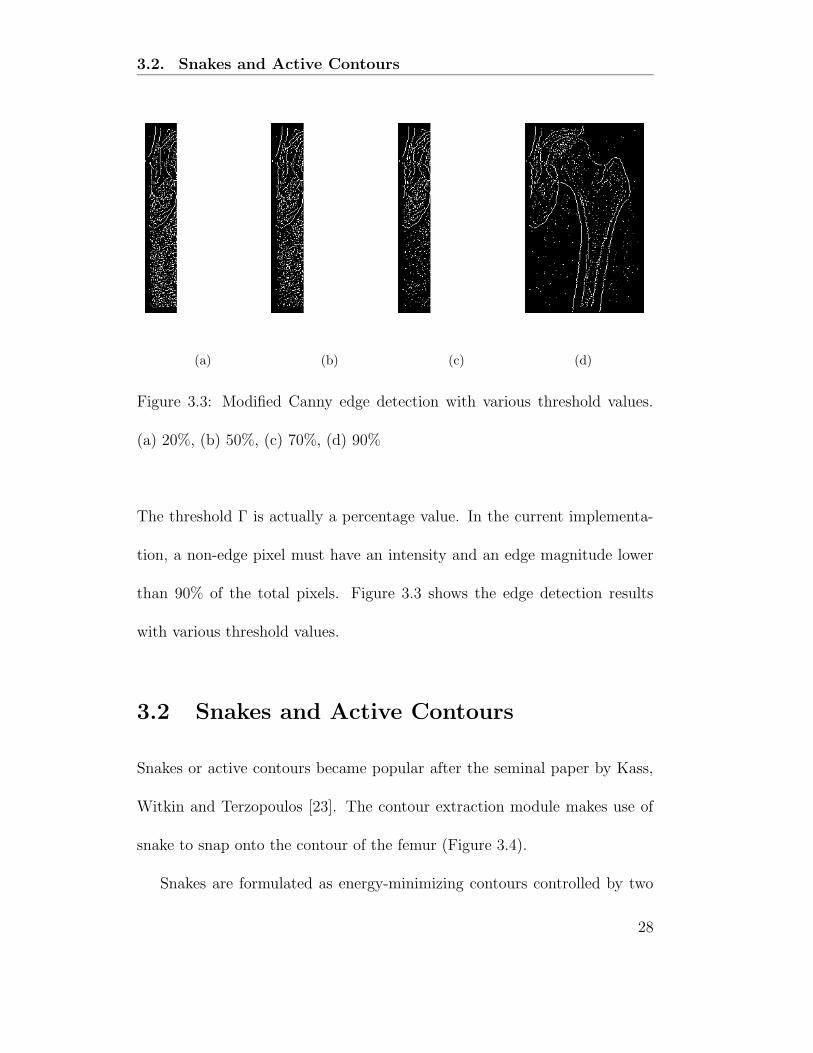
tude values are removed (Figure 3.3d).
In summary, a pixel is marked as an non-edge point if
1. it is detected by Canny edge detector,
2. it has an intensity lower than a threshold Γ, and
3. it has an edge magnitude lower than the same threshold Γ.
27
3.2. Snakes and Active Contours
(a) (b) (c) (d)
Figure 3.3: Modified Canny edge detection with various threshold values.
(a) 20%, (b) 50%, (c) 70%, (d) 90%
The threshold Γ is actually a percentage value. In the current implementa-
tion, a non-edge pixel must have an intensity and an edge magnitude lower
than 90% of the total pixels. Figure 3.3 shows the edge detection results
with various threshold values.
3.2 Snakes and Active Contours
Snakes or active contours became popular after the seminal paper by Kass,
Witkin and Terzopoulos [23]. The contour extraction module makes use of
snake to snap onto the contour of the femur (Figure 3.4).
Snakes are formulated as energy-minimizing contours controlled by two
28

3.2. Snakes and Active Contours
forces:
1. Internal contour forces which enforce the smoothness constraint.
2. Image forces which attracts the contour to the desired features, in this
case, edges.
Esnake =
∫
1
0
Eint(v(s)) + Eimage(v(s))ds (3.1)
Representing the position of the snake parametrically by v(s) = (x(s), y(s)),
the energy of a snake Esnake (Eqn 3.1) is a sum of the internal energy Eint
of the snake and the image energy Eimage.
Internal Energy
The internal energy Eint is composed of a first-order term controlled
by α(s) and a second order term controlled by β(s).
Eint =(
α(s) |vs(s)|2 + β(s) |vss(s)|
2)
/2 (3.2)
The terms vs and vss represents the first and second derivative of v
respectively. α(s) characterizes the tension along the snake and β(s)
characterizes the bending of the curve. Currently, α(s) and β(s) are
set as values α and β.
29
3.2. Snakes and Active Contours
Image Energy
In the current implementation, the snake is programmed to converge
onto edges and modified Canny edge detector (Section 3.1) is used
to compute the edges Eedge from the input images. The image en-
ergy Eimage will be Eedge weighted appropriately by a negative weight
−wedge.
Eimage = −wedgeEedge (3.3)
Minimization Procedure
A snake that minimize the energy functional Esnake must satisfy the
following Euler equations [23] :
αxss + βxssss +∂Eimage
∂x= 0 (3.4)
αyss + βyssss +∂Eimage
∂y= 0 (3.5)
Where xss and xssss are the second and fourth derivatives of x, similarly
for yss and yssss.
In computer implementation, Eqn 3.1 is discretized as follows :
Esnake =n
∑
i=1
Eint(i) + Eimage(i) (3.6)
Using a vector notation with vi = (xi, yi) = (x(ih), y(ih)) and approxi-
mating the derivatives xss, xssss, yss and yssss in Eqn 3.4 and 3.5 using
30

3.2. Snakes and Active Contours
finite difference, Eint(i) can be expanded as :
Eint(i) =αi |vi − vi−1|
2
2h2+
βi |vi−1 − 2vi + vi+1|2
2h4(3.7)
For a closed contour snake, we can define v(0) = v(n). Define fx(i) =
∂Eimage/∂xi and fy(i) = ∂Eimage/∂yi where the derivatives are approxi-
mated by finite difference. Therefore the corresponding Euler equations
(Eqn 3.4, 3.5) become
αi(vi − vi−1)− αi+1(vi+1 − vi) + βi−1(vi−2 − 2vi−1 + vi)
− 2βi(vi−1 − 2vi + vi+1) + βi+1(vi − 2vi+1 + vi+2) + (fx(i), fy(i)) = 0
(3.8)
Rewriting the above Euler equations in matrix form we have
Ax + fx(x,y) = 0 (3.9)
Ay + fy(x,y) = 0 (3.10)
Where A is a penta-diagonal banded matrix and below is an examplefor a 7 point closed contour with constant α and β :
A =
c1 d1 e1 0 0 a1 b1
b2 c2 d2 e2 0 0 a2
a3 b3 c3 d3 e3 0 00 a4 b4 c4 d4 e4 00 0 a5 b5 c5 d5 e5
e6 0 0 a6 b6 c6 d6
d7 e7 0 0 a7 b7 c7
ai = βi−1
bi = −αi − 2βi−1 − 2βi
ci = αi + αi+1 + βi−1 + 4βi + βi+1
di = −αi+1 − 2βi − 2βi+1
ei = βi+1
(3.11)
To solve Eqn 3.9, the snake is made dynamic by treating x and y as
31

3.3. Gradient Vector Flow
function of time and solved iteratively [23].
x(t + 1) = (A + γI)−1(γx(t)− fx(x(t),y(t))) (3.12)
y(t + 1) = (A + γI)−1(γy(t)− fx(x(t),y(t))) (3.13)
where γ is the Euler step size. (A + γI)−1 can be calculated by LU
decomposition in O(n) time, where n is the length of the snake.
3.3 Gradient Vector Flow
Gradient Vector Flow (GVF) [34] is a type of external force for active con-
tours. The GVF was created to overcome two shortcomings of the original
active contour formulation i.e poor convergence to concave boundaries and
sensitivity to initialization. GVF is computed as a diffusion of the gradient
vectors of a gray-level edge map derived from the image.
The GVF field is defined as the vector field G(x, y) = (q(x, y), r(x, y))
that minimizes the energy functional
ε =
∫ ∫
µ(q2
x + q2
y + r2
x + r2
y) + |∇E|2 |G−∇E|2 dxdy (3.14)
where E is an edge map E(x, y) derived from the image. Using calculus of
variations, the GVF can be found by solving the following Euler equations
32

3.4. Combining Snake with GVF
µ∇2q− (q−E2
x + E2
y) = 0 (3.15)
µ∇2r− (r−E2
y + E2
y) = 0 (3.16)
Equations 3.15 and 3.16 can be solved by treating q and r as functions
of time and solving
q(x, y, t + 1) =µ∇2q(x, y, t)
− (q(x, y, t)− Ex(x, y)) · (Ex(x, y)2 + Ey(x, y)2)
(3.17)
r(x, y, t + 1) =µ∇2r(x, y, t)
− (r(x, y, t)−Ey(x, y)) · (Ex(x, y)2 + Ey(x, y)2)
(3.18)
The steady state solution (as t → ∞) of equations 3.17 and 3.18 is the
require solution of the Euler equations 3.15 and 3.16. Details of the numerical
implementation for Eqn 3.15 and 3.16 can be found in [35].
3.4 Combining Snake with GVF
The snake algorithm is combine with the external force computed by the GVF
to improve the performance of snake. To incorporate the GVF into the snake
algorithm, after computing the solution q and r in equation 3.17 and 3.18,
replace fx and fy from equation 3.12 and 3.13 with q and r respectively.
With the GVF snake, only a small number of initialization points are
needed to start the snake algorithm (Figure 3.4) and successive iterations
33

3.4. Combining Snake with GVF
of the algorithm will re-distribute the snake points more regularly along the
contours.
(a) (b) (c)
Figure 3.4: With small number of initialization points in (a) an accurate
outline of the femur can be obtained using snake combine with GVF (b). (c)
shows the result of using snake without GVF and it is difficult to get the
snake to snap onto the concave structure at the femoral neck.
34
Chapter 4
Measuring Neck-Shaft Angle
from Femur Contour
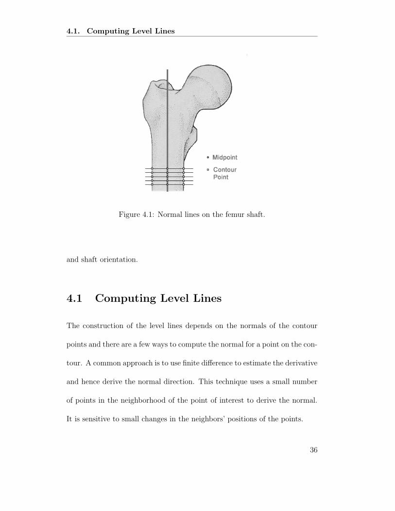
The contour lines along the femoral shaft are almost parallel. If normal lines
are drawn from one side of the shaft to the opposite side and compute the
midpoints of these lines, then the mid-points would be aligned parallel to the
shaft (Figure 4.1). We call these normal lines level lines as each line denotes
a level along the femoral shaft. Section 4.1 will explain in detail how such
lines are constructed and Section 4.2 will how the midpoints of the level lines
are used to determine the orientation of the shaft. The level lines are also
useful for computing the orientation of the femoral neck, which is elaborated
in Section 4.3. Once the shaft orientation and the neck orientation have been
computed, the neck-shaft angle can be easily computed as the angle the neck
4.1. Computing Level Lines
Figure 4.1: Normal lines on the femur shaft.
and shaft orientation.
4.1 Computing Level Lines
The construction of the level lines depends on the normals of the contour
points and there are a few ways to compute the normal for a point on the con-
tour. A common approach is to use finite difference to estimate the derivative
and hence derive the normal direction. This technique uses a small number
of points in the neighborhood of the point of interest to derive the normal.
It is sensitive to small changes in the neighbors’ positions of the points.
36

4.1. Computing Level Lines
On the other hand, with a dense sampling of points along the contour,
a larger set of points can be used to compute the normal at a point using
Principal Component Analysis (PCA) [21, 22]. To compute the normal of a
contour point, choose a neighborhood of points around the point of interest.
This set of points represents a segment of the contour and PCA is applied to
this segment of points. Given a set of points in 2D, PCA returns two eigen-
vectors and their associated eigenvalues. The eigenvector with the largest
eigenvalue will point in the direction parallel to this segment of points and
the other eigenvector gives the normal direction at the point of interest.
Once the normal for each point on the contour has been calculated, the
set of level lines L can be computed. Let pi and pj denote the vector repre-
sentation of two points on the contour and ni and nj be the associated unit
normals. Then the line l(pi,pj) that connects points pi and pj is a level line
if
|ni · nj| ≈ |(pi − pj) · ni| ≈ |(pi − pj) · nj| ≈ 1 (4.1)
In the current implementation, two orientations v1 and v2 are similar i.e.,
|v1 · v2| ≈ 1 if |v1 · v2| ≥ 0.98
37
4.2. Computing Orientation of the Femoral Shaft
4.2 Computing Orientation of the Femoral
Shaft
The orientation of the femur shaft can be computed by extracting the mid-
points of the level lines on the shaft (Figure 4.2). Given level lines li(p1i ,p
2i )
and the midpoints mi = 1
2(p1
i + p2i ), sort mi in decreasing order of y-
coordinates of mi (assuming the origin is at the top-left corner of the image)
and call them m′
i. The first midpoint m′
1 must be a midpoint along the
femoral shaft. Now for each midpoint m′
i, i ≥ 2, include m′
i as a shaft point
if m′
i is near to m′
i−1.
After finding the midpoints of the shaft, the PCA algorithm is used to
estimate the orientation of the midpoints. The eigenvector with the largest
eigenvalue computed from the PCA algorithm will represent the orientation
of the shaft midpoints.
4.3 Computing the Orientation of the Femoral
Neck
The computation of femoral neck’s orientation is more complicated because
there is no obvious axis of symmetry. The algorithm consist of three main
steps.
38

4.3. Computing the Orientation of the Femoral Neck
Figure 4.2: The midpoints of the level lines are shown as white dots. The
midpoints along the shaft give a good estimate of the orientation of the
femoral shaft.
39

4.3.1 Computing Initial Estimation of Femoral Neck’s Orientation
1. compute an initial estimate of the neck orientation (Section 4.3.1) ,
2. smooth the femur contour (Section 4.3.2), and
3. search for the best axis of symmetry using the initial neck orientation
estimate (Section 4.3.3).
4.3.1 Computing Initial Estimation of Femoral Neck’s
Orientation
The longest level lines in the upper region of the femur always cut through the
contour of the femoral head (Figure 4.3). Given this observation, an adaptive
clustering algorithm [24] is used to cluster long level lines at the femoral head
into bundles of closely spaced level lines with similar orientations. The bundle
with the largest number of lines is chosen, and the average orientation of the
level lines in this bundle is regarded as the initial estimate of the orientation
of the femoral neck.
The adaptive clustering algorithm is useful as it does not need to choose
the number of clusters before hand. The general idea is to group the level
lines such that in each group, the level lines are similar in terms of orientation
and spatial position. The adaptive clustering algorithm groups a level line
into its nearest cluster if the orientation and midpoint of the cluster is close.
If a level line is far enough from any of the existing clusters, a new cluster
40

4.3.1 Computing Initial Estimation of Femoral Neck’s Orientation
Figure 4.3: Level lines along the femoral neck intersects the femoral head
contour.
will be created for this level line. For level lines that are neither close nor far
enough, they will be left alone and not assigned to any cluster.
With the adaptive clustering algorithm, it ensures each cluster has a
minimum similarity of R1 for the cluster orientation and minimum similarity
of R2 for the mid-points distance. The algorithm also ensures that the cluster
differs by a similarity of at most S1 and S2 for the orientation and mid-points
distance respectively. Varying the values of R1, R2, S1 and S2 controls the
41

4.3.2 Smoothing the Original Contour
granularity of clustering and the amount of overlapping between clusters.
Algorithm 1: Computing initial estimation of femoral neck’s orienta-tion.
Input: Set of level lines L = {li}, with corresponding orientation ui
and midpoint mi.
Output: A point phead on the femoral head contour.
Note that each cluster k is characterized by an orientation uk and amidpoint mk.
1 foreach li ∈ L do
Find cluster k such that orientation uk is most similar to ui andmk is close to mi.If |uk · ui| ≥ R1 and |mi −mk| ≤ R2 (i.e similar in orientationand spatially close).Then include li in cluster kElse if |uk · ui| ≤ S1 and |mi −mk| ≥ S2
Then create a new cluster with line li.end
2 Update cluster orientation and midpointRepeat 1 and 2 until convergence
4.3.2 Smoothing the Original Contour
Consider a parametric equation for a curve v = (x(s), y(s)) and g(s, σ) is
a 1-D Gaussian kernel of width σ then X(s, σ) and Y (s, σ) represents the
components of a smoothed curve,
X(s, σ) = x(s) ∗ g(s, σ) (4.2)
Y (s, σ) = y(s) ∗ g(s, σ) (4.3)
42

4.3.3 Computing the Axis of Symmetry for the Femoral Head and
Neck
(a) Original (b) σ = 2 (c) σ = 6 (d) σ = 10
Figure 4.4: Contour smoothing. (a) Original femur contour. (b,c,d) smooth
contours with different σ.
Observe that in Figure 4.4(c) the outline of the femoral head and neck is
almost symmetrical after sufficient smoothing has been applied to the curve.
The algorithm exploits this symmetry to estimate the orientation of the neck.
Currently σ is chosen to be 5.
4.3.3 Computing the Axis of Symmetry for the Femoral
Head and Neck
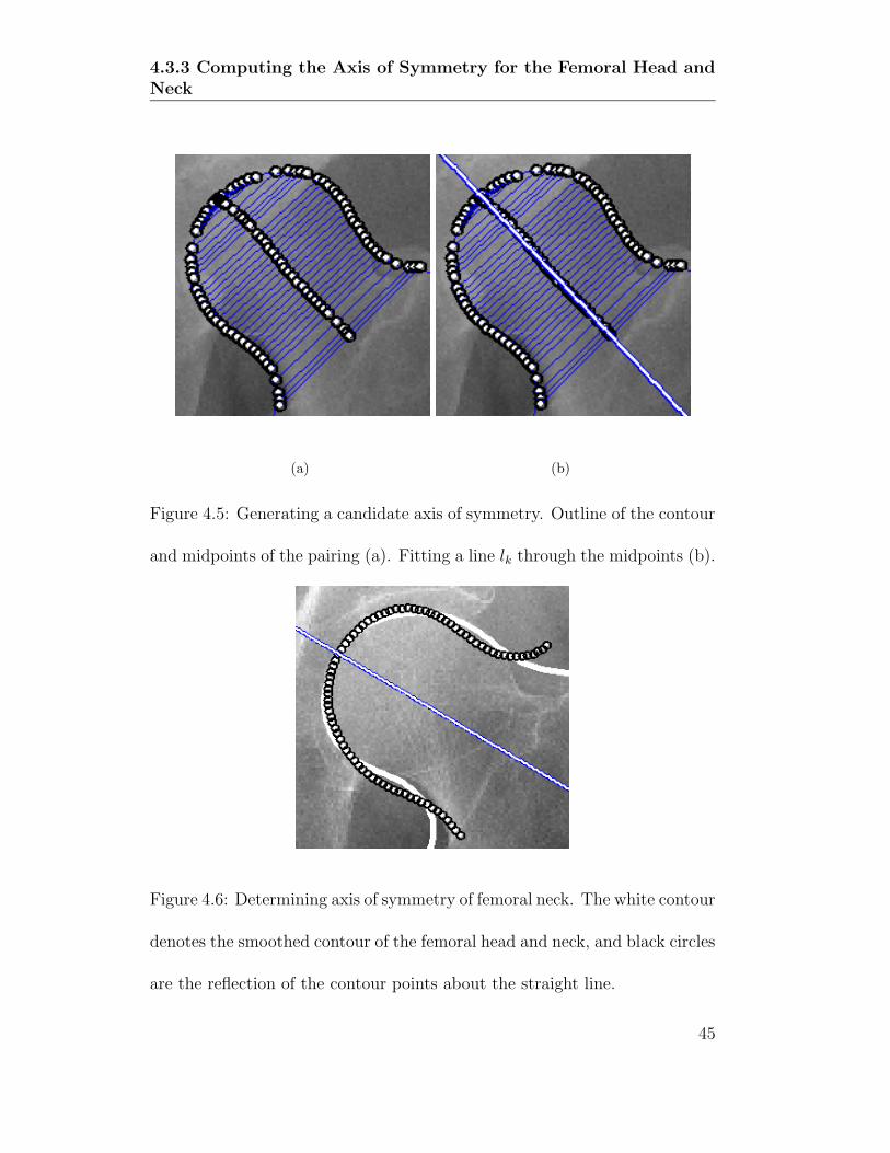
The general idea of determining the axis of symmetry is to find a line through
the femoral neck and head such that the contour of the head and neck coin-
cides with its own reflection about the line (Figure 4.6).
43
4.3.3 Computing the Axis of Symmetry for the Femoral Head and
Neck
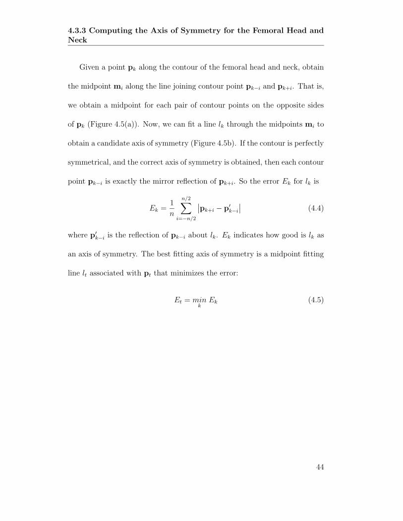
Given a point pk along the contour of the femoral head and neck, obtain
the midpoint mi along the line joining contour point pk−i and pk+i. That is,
we obtain a midpoint for each pair of contour points on the opposite sides
of pk (Figure 4.5(a)). Now, we can fit a line lk through the midpoints mi to
obtain a candidate axis of symmetry (Figure 4.5b). If the contour is perfectly
symmetrical, and the correct axis of symmetry is obtained, then each contour
point pk−i is exactly the mirror reflection of pk+i. So the error Ek for lk is
Ek =1
n
n/2∑
i=−n/2
∣
∣pk+i − p′
k−i
∣
∣ (4.4)
where p′
k−i is the reflection of pk−i about lk. Ek indicates how good is lk as
an axis of symmetry. The best fitting axis of symmetry is a midpoint fitting
line lt associated with pt that minimizes the error:
Et = mink
Ek (4.5)
44
4.3.3 Computing the Axis of Symmetry for the Femoral Head and
Neck
(a) (b)
Figure 4.5: Generating a candidate axis of symmetry. Outline of the contour
and midpoints of the pairing (a). Fitting a line lk through the midpoints (b).
Figure 4.6: Determining axis of symmetry of femoral neck. The white contour
denotes the smoothed contour of the femoral head and neck, and black circles
are the reflection of the contour points about the straight line.
45

Chapter 5
Test Results and Discussion
Manual measurement of neck-shaft angles turns out to be quite inconsistent.
So, there is no accurate and consistent ground truth for assessing the accuracy
of the algorithm that measures the neck-shaft angle. Instead, experiments
are conducted to determine how accurate can the measured neck-shaft angle
be used to distinguish healthy femurs from fractured femur.
5.1 Classification using Neck-Shaft Angle
5.1.1 Test Setup
A set of 64 radiographic images of the hip were obtained. Of these 64 hip
images, 19 of them contained fractures. Out of the 19 hip fractures, 12 were
left femur fractures and 7 were right femur fractures. Each image contains

5.1.2 Test Results
at most one fracture.
Three measurements were taken for each radiographic image: the neck-
shaft angles for the left and right femur and the absolute difference between
the left and right neck-shaft angles. The doctors frequently compare the
left and right femur to look for significant differences between them. Hence,
another classification will be based on the difference of the left and right
neck-shaft angles.
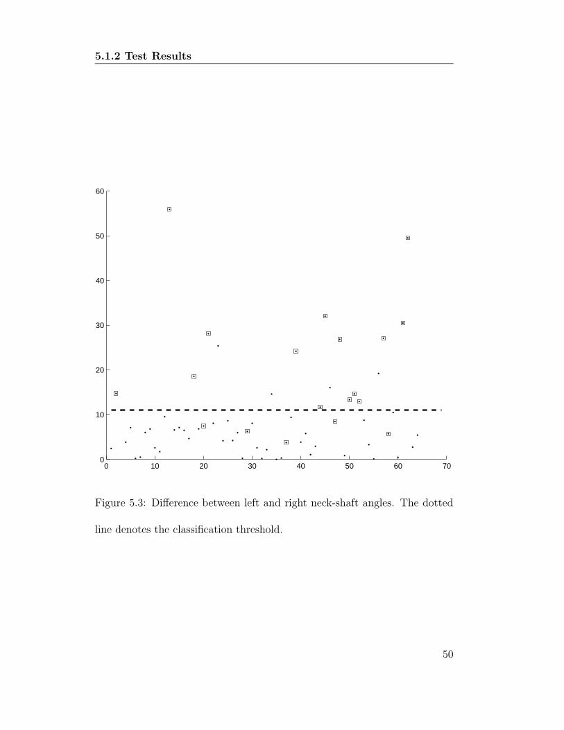
5.1.2 Test Results
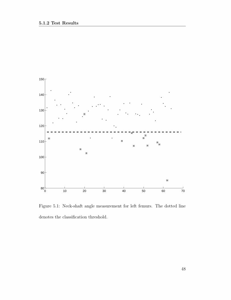
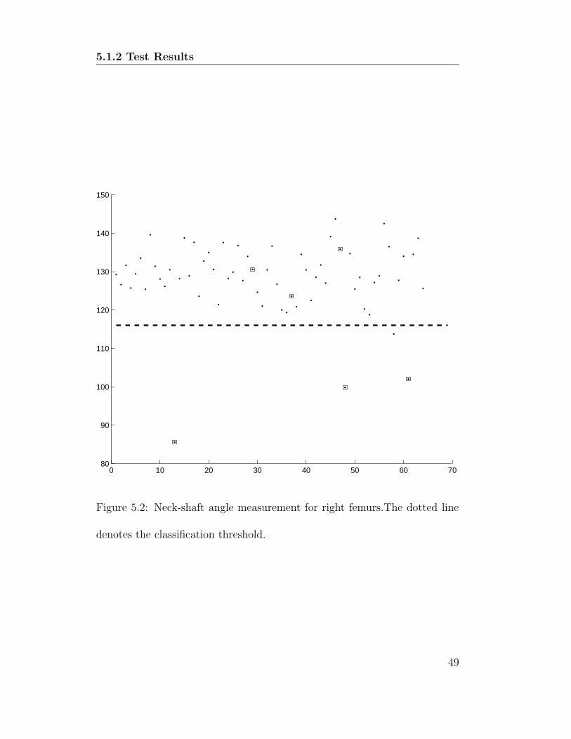
A summary of the result of running neck-shaft angle measurement of the
left and right femurs can be found in Figure 5.1 and Figure 5.2 respectively.
The summary for the difference of left and right neck-shaft angles is shown
in Figure 5.3. The x-axis represents the different test cases and the y-axis
represents the neck-shaft angle measured in degrees. The dots represent the
healthy femurs and the box around a dot denotes that the femur is fractured.
From Figure 5.1 and Figure 5.2, we can see that setting a threshold at 116
degrees yields the best classification accuracy. For the left-right difference,
Figure 5.3 shows that a threshold of 11 degrees yields the best classification
accuracy.
A summary of the classification results can be found in Table 5.1. The sec-
47
5.1.2 Test Results
0 10 20 30 40 50 60 7080
90
100
110
120
130
140
150
Figure 5.1: Neck-shaft angle measurement for left femurs. The dotted line
denotes the classification threshold.
48
5.1.2 Test Results
0 10 20 30 40 50 60 7080
90
100
110
120
130
140
150
Figure 5.2: Neck-shaft angle measurement for right femurs.The dotted line
denotes the classification threshold.
49
5.1.2 Test Results
0 10 20 30 40 50 60 700
10
20
30
40
50
60
Figure 5.3: Difference between left and right neck-shaft angles. The dotted
line denotes the classification threshold.
50

5.1.2 Test Results
Left Femur Right Femur Left & Right Difference
Correct Classification
as fracture 12 3 15 14
as healthy 49 57 106 41
sub-total 61 (95.3%) 60 (93.8%) 121 (94.5%) 55 (85.9%)
Wrong classification
as fracture 2 1 3 4
as healthy 1 3 4 5
sub-total 3 (4.7%) 4 (6.2%) 7 (5.5%) 9 (14.1%)
Total 64 64 128 64
Table 5.1: Summary of classification results.
51

5.1.3 Discussion on Classification Results
ond column contains the result for the left femur, the third column contains
the result for the right femur and the fourth column contains the combined
results for the left and right femur. The fifth column shows the results using
the neck-shaft angle difference.
Using a neck-shaft angle thresholding classifier, we can achieve an ac-
curacy of 95.3% and 93.8% for the left and right femurs respectively. The
overall accuracy for all the femurs is 94.5%. Misclassification rate is 4.7% for
the left femur and 6.2% for the right femur. The combined misclassification
rate is 5.5%. Out of 19 fractured cases, the classifier manages to detect 15
correctly (i.e, 80% of the total number of fractured femurs) and 4 are are
wrongly classified as healthy.
Using the neck-shaft angle difference between the left and right femurs
to classify the radiographic images, 55 images were correctly classified and
accuracy for correct classification is 85.9%. For the misclassifications, out of
55 images, 4 images were wrongly classified.
5.1.3 Discussion on Classification Results
The algorithm has performed very well in classifying individual femurs based
on neck-shaft angle. For example, for the femurs in Figure 5.4, the neck
shaft angles were correctly measured and correctly classified as healthy. The
52
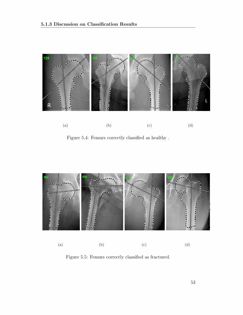
5.1.3 Discussion on Classification Results
(a) (b) (c) (d)
Figure 5.4: Femurs correctly classified as healthy .
(a) (b) (c) (d)
Figure 5.5: Femurs correctly classified as fractured.
53

5.1.3 Discussion on Classification Results
(a) (b) (c) (d)
Figure 5.6: Fractured femurs in (a) and (b) are wrongly classified as healthy
due to small change in neck-shaft angle. Fractured femurs in (c) and (d) are
wrongly classified as there is no change in neck-shaft angle.
femurs in Figure 5.5 were correctly classified as fractured and the neck-shaft
angles were also correctly measured. There are two main reasons for the
misclassification of fractured femurs as healthy femurs. The first reason is
due to the fact that the fractures are not severe enough to change the neck-
shaft angle significantly. For example in Figure 5.6(a) and (b) both femurs are
fractured at the intertrochanteric region but the change in neck-shaft angle
is not significant enough to be detected by the classified. For the second
type of misclassification, a fracture has occurred but there is no change in
neck-shaft angle of the femur. For example, in Figure 5.6(c) and (d). Such
54
5.1.3 Discussion on Classification Results
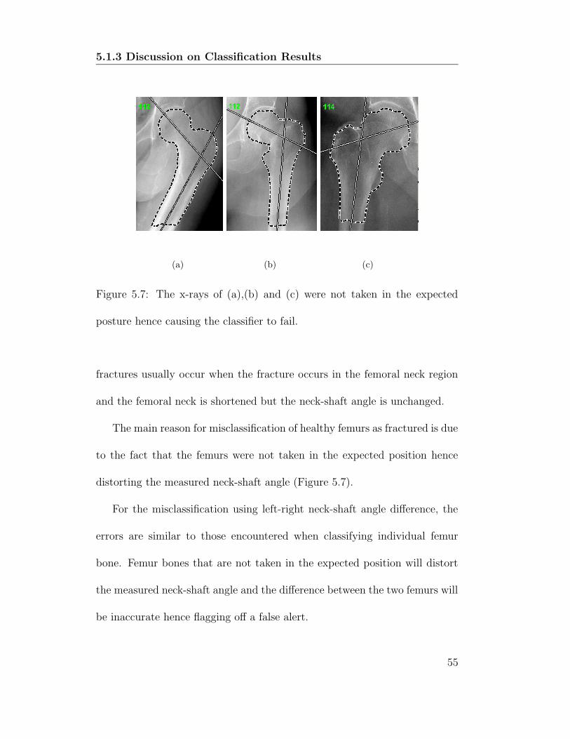
(a) (b) (c)
Figure 5.7: The x-rays of (a),(b) and (c) were not taken in the expected
posture hence causing the classifier to fail.
fractures usually occur when the fracture occurs in the femoral neck region
and the femoral neck is shortened but the neck-shaft angle is unchanged.
The main reason for misclassification of healthy femurs as fractured is due
to the fact that the femurs were not taken in the expected position hence
distorting the measured neck-shaft angle (Figure 5.7).
For the misclassification using left-right neck-shaft angle difference, the
errors are similar to those encountered when classifying individual femur
bone. Femur bones that are not taken in the expected position will distort
the measured neck-shaft angle and the difference between the two femurs will
be inaccurate hence flagging off a false alert.
55

Chapter 6
Future Work
In summary, the two main reasons for misclassification are:
1. Insufficient deformation in the shape to cause a large change in the
neck-shaft angle
2. Fractured femurs with no change in neck-shaft angle.
To solve problem (1) it is suggested that other ways of detecting fractures be
tried. For example, another feature to extract for diagnosing femur fractures
is the texture of trabecular lines (Figure 6.1). Such lines run from the shaft
of the femur through the neck and ending near the head of the femur. A
fracture in the neck of the femur will usually disrupt the smooth running of
these lines and an analysis of such pattern to pick up any major changes in
the trabecular pattern is useful for locating the fracture site.

Figure 6.1: Trabecular lines.
To solve problem (2) other measurements of the femur bone have to be
taken. An example will be measuring the ratio of the length of the femur
neck to other parts of the femur.
With the algorithms proposed, the neck-shaft angle of a front-view x-ray
image of the femur can be calculated. A more accurate method of measuring
neck-shaft angle can be computed using two x-ray images. The second x-ray
is taken at an oblique angle to the first. This approach takes into account 3D
structure of the femur bone and based on the projection of the femur bone
on two different planes the neck shaft angle in 3D can be computed. This
method have been used in [28] to manually measure the neck-shaft angles in
57

young patients.
58

Chapter 7
Conclusion
In this thesis, we study the problem of estimating neck-shaft angle from the
contour of the femur. A method is proposed to compute neck-shaft angle.
The method comprises two algorithms. The first algorithm extracts the femur
contour accurately from x-Ray images and the second algorithm computes
neck-shaft angle based on the contour of the femur. The contributions of this
research includes the following :
1. Developing two algorithms that form the core of a system to assist
doctors in detecting femur fractures.
2. A computational method of measuring the neck-shaft angle which is
more consistent and reproducible compared to manual measurement.

To the best of our knowledge, this is the first computer algorithm for
measuring the neck-shaft angle from x-ray images and using neck-shaft angle
to discriminate healthy femurs from fractured femurs. From the experiments
conducted, we have shown that using the neck-shaft angle measured by our
algorithm we can achieve a classification accuracy of 94.5%. In summary, this
research has provided a basis for future research in femur fracture detection
and developing algorithms to assist doctors in diagnosing fractures.
60

Bibliography
[1] A. Amini, T. Weymouth, and R. Jain. Using dynamic programming for
solving variational problems in vision. IEEE Transaction on Pattern
Analysis and Machine Intelligence, 12(9):855–867, 1990.
[2] Y. Amit. Graphical shape templates for automatic anatomy detection
with applications to MRI brain scans. IEEE Transactions on Medical
Imaging, 16(1), February 1997.
[3] Y. Amit and A. Kong. Graphical template for model registration. IEEE
Transaction on Pattern Analysis and Machine Intelligence, 18(3), March
1996.
[4] H. Asada and M. Brady. The curvature primal sketch. IEEE Transac-
tions on Pattern Analysis and Machine Intelligence, 8(1):2–14, January
1986.

Bibliography
[5] G. Behiels, F. Maes, D. Vandermeulen, and P. Suetens. Evaluation
of image features and search strategies for segmentation of bone struc-
tures in radiographs using active shape models. Medical Image Analysis,
6(1):47–62, March 2002.
[6] F. L. Bookstein. Landmark methods for forms without landmarks :
Morphometrics of group differences in outline shape. Medical Image
Analysis, 1(3):225–243, 1997.
[7] J. Canny. A computational approach to edge detection. IEEE Trans-
actions on Pattern Analysis and Machinie Intelligence, 8(6):679–698,
1986.
[8] C. C. Change, S. M. Hwang, and D. J. Buehrer. A shape recognition
scheme based on relative distances of feature points from the centroid.
Pattern Recognition, 1991.
[9] L. D. Cohen. Note on active contour models and ballons. CVGIP :
Image Understanding, 53(2):211–218, March 1991.
[10] L. D. Cohen and I. Cohen. Finite-element methods for active contour
models and ballons for 2-D and 3-D images. IEEE Transaction on Pat-
tern Analysis and Machine Intelligence, 15(11):1131–1147, 1993.
62

Bibliography
[11] T. Cootes and C. J. Taylor. Statistical models of appearance for com-
puter vision. Draft report, available at http://www.wiau.man.ac.uk,
1999.
[12] T. F. Cootes, A. Hill, C. J. Taylor, and J. Haslam. Use of active shape
models for locating structres in medical images. Image Vision Comput-
ing, 12:355–365, 1994.
[13] T. F. Cootes, C. J. Taylor, and D. H. Cooper. Active shape models - their
training and application. Computer Vision and Image Understanding,
61(1), January 1995.
[14] T. F. Cootes, C. J. Taylor, D. H. Cooper, and J. Graham. Training
models of shape from sets of examples. In Proc. of British Machine
Vision Conference, pages 9–18. Springer-Verlag, 1992.
[15] I. L. Dryden and K. V. Mardia. Statistical Shape Analysis. John Wiley
& Sons, 1998.
[16] P. J. Evans and B. J. McGrory. Fractures of the proximal femur. Hospital
Physician, April 2002.
[17] P. Golland and W. E. L. Grimson. Fixed topology skeletons. In Proc.
of IEEE Computer Vision and Pattern Recognition, pages 10–17, 2000.
63

Bibliography
[18] C. Goodall. Procrustes methods in the statistical analysis of shape.
Journal of the Royal Statistical Society B, 53:285–339, 1991.
[19] J. S. Gregory, D. Testi, R. E. Undrill, and R. M. Aspden. Hip fractures,
morphometry and geometry. In Proc. of 29th European Symposium on
Calcified Tissues, 2002.
[20] L. Gupta, M. R. Sayeh, and R. Tammana. A neural network approach
to robust shape classification. Pattern Recognition, 1990.
[21] S. Haykin. Neural Networks: A Comprehensive Foundation. Prentice-
Hall, 2nd edition, 1991.
[22] I. T. Jolliffee. Principal Component Analysis. Springer Verlag, 1996.
[23] M. Kass, A. Witkin, and D. Terzopoulos. Snakes: Active contour mod-
els. International Journal of Computer Vision, 1:321–331, 1988.
[24] W. K. Leow and R. Li. Adaptive binning and dissimilarity measure for
image retrieval and classification. In Proc. of IEEE Computer Vision
and Pattern Recognition, 2001.
[25] K. V. Mardia, J. T. Kent, and A. N. Walder. Statistical shape models
in image analysis. In E Keramidas, editor, Proc. of Computer Science
and Statistics : 23rd INTERFACE Symposium, pages 550–557, 1991.
64
Bibliography
[26] F. Mokhtarian and A. Mackworth. Scale-based description and recogni-
tion of planar curves and two dimensional shapes. IEEE Transactions on
Pattern Analysis and Machine Intelligence, 8(1):34–43, January 1986.
[27] F. Mokhtarian and H. Muraase. Silhouette-base object recognition
through curvature scale space. In Proc. of International Conference
on Computer Vision, pages 269–274, 1993.
[28] K. Ogata and E. M. Goldsand. A simple biplanar method of measuring
femoral anteversion and neck shaft angle. The Journal of Bone and
Joint Surgery, 61-A(6):846–851, 1979.
[29] S. M. Pizer, D. H. Eberly, B. S. Morse, and D. S. Fritsch. Zoom invariant
vision of figural shape: The mathematics of cores. Computer Vision
Image Understanding, 69:55–71, 1998.
[30] S. M. Pizer, D. Fritsch, P. A. Yushkevich, V. E. Johnson, and E. L.
Chaney. Segmentation, registration and measurement of shape variation
via image object shape. IEEE Transactions on Medical Imaging, 18, Oct
1999.
[31] D. Terzopolous, J. Platt, A. Barr, and K. Fleischer. Elastically de-
formable models. Computer Graphics, 21(4):205–214, 1987.
65
Bibliography
[32] D. Terzopolous, A. Witkin, and M. Kass. Constraints on deformable
models : recovering 3D shape and nonrigid motion. Artificial Intelli-
gence, 36:91–123, 1988.
[33] M. K. Wong, Arjandas, L. K. Ching, S. L. Lim, and N. N. Lo. Osteo-
porotic hip fractures in Singapore - costs and patient’s outcome. Ann
Acad Med Singapore, 2002.
[34] C. Xu and J. L. Prince. Gradient vector flow : A new external force for
snakes. In Proc. of IEEE Conference on Computer Vision and Pattern
Recognition, 1997.
[35] C. Xu and J. L. Prince. Snakes,shapes, and gradient vector flow. IEEE
Transactions on Image Processing, 1997.
[36] A. L. Yuille, P. W. Hallinan, and D. S. Cohen. Feature extraction from
faces using deformable templates. International Journal of Computer
Vision, 8:99–111, 1992.
66