Detection of 106Ru, via the decay of its daughter 106Rh, in gamma-ray spectra

Technical considerations

for laboratory work

Mikael Hult and Guillaume Lutter

EUR 28850 EN

2017

xxxxx xx

This publication is a Technical report by the Joint Research Centre (JRC), the European Commission’s science

and knowledge service. It aims to provide evidence-based scientific support to the European policymaking

process. The scientific output expressed does not imply a policy position of the European Commission. Neither

the European Commission nor any person acting on behalf of the Commission is responsible for the use that

might be made of this publication.

Contact information

Name: M. Hult

Address: Retieseweg 111, 2440 Geel, Belgium

Email: Mikael.hult@ec.europa.eu

Tel.: +32-14-571 269

JRC Science Hub

https://ec.europa.eu/jrc

JRC108853

EUR 28850 EN

PDF ISBN 978-92-79-74675-8 ISSN 1831-9424 doi:10.2760/62038

Luxembourg: Publications Office of the European Union, 2017

© European Atomic Energy Community, 2017

Reuse is authorised provided the source is acknowledged. The reuse policy of European Commission documents is regulated by Decision 2011/833/EU (OJ L 330, 14.12.2011, p. 39).

For any use or reproduction of photos or other material that is not under the EU copyright, permission must be

sought directly from the copyright holders.

How to cite this report: Mikael Hult and Guillaume Lutter, Detection of 106Ru, via the decay of its daughter 106Rh,

in gamma-ray spectra : Technical considerations for laboratory work, EUR 28850 EN, Publications Office of the

European Union, Luxembourg, 2017, ISBN 978-92-79-74675-8, doi 10.2760/62038, Pubsy No. 108853

All images © European Atomic Energy Community 2017, except:

The table in Annex I, which is from the online database at www.nucleide.org and more specifically

http://www.nucleide.org/DDEP_WG/Nuclides/Rh-106_tables.pdf. It is being maintained by Laboratoire National

Henri Becquerel (CEA/LNHB), att. Mark Kellet, 91191 Gif-sur-Yvette, Cedex, France, from where permission

was obtained.

3

Objective

This report gives a brief overview of some key aspects to consider when searching for 106Ru in gamma-ray spectra from environmental samples and what to keep in mind when producing quantitative activity-results in the unit Bq.

1 Ruthenium-106 and daughter

Ruthenium-106 (106Ru) is a pure beta-minus emitter with a half-life of 371.5 days. It decays to the ground state of rhodium-106 (106Rh). The half-life of 106Rh is only 30.1 seconds so in any sample measured in a laboratory, there should be secular equilibrium between 106Ru and 106Rh after only a few minutes. This means that they decay at the same rate and have the same activity1.

Rhodium-106 is also a pure beta-minus emitter, but in contrast to its parent, its decay is followed by emission of gamma-rays from deexcitations of its daughter-nucleus 106Pd. These gamma-rays can be used for detecting 106Rh, and consequently also indirectly 106Ru, using gamma-ray spectrometry.

The decay data of 106Ru and 106Rh, which is recommended by the ICRM (International Committee for Radionuclide Metrology), can be found at the DDEP (Decay Data Evaluation Project) website with data from Bé et al. (2016).

http://www.nucleide.org/DDEP_WG/DDEPdata.htm

http://www.nucleide.org/DDEP_WG/Nuclides/Rh-106_tables.pdf

http://www.nucleide.org/DDEP_WG/Nuclides/Ru-106_tables.pdf

2 Gamma-ray spectrum

Examples of gamma-ray spectra using both germanium-detectors as well as NaI detectors2 can be found online at Idaho National Laboratory's (INL) webpage: http://www4vip.inl.gov/gammaray/catalogs/catalogs.shtml In INL's spectra of 106Ru and 106Rh, the source is located 10 cm above the detector.

In Figure 1 is shown a simulated gamma-ray spectrum from 106Rh, homogeneously distributed in a 5 mm thick sample made of several circular filters inside a polycarbonate container that is placed directly on the endcap of the detector. The close geometry results in much coincidence summing (see Chapter 4), which is not the case in the spectrum at the INL website. In a similar (but opposite) manner is the effect of angular correlation (see Chapter 5) stronger in the INL spectrum whilst almost negligible in the spectrum of Figure 1.

1 This means that if a laboratory claims a massic activity of for example 10 Bq/kg of 106Rh, there is in fact 20 Bq/kg of 106Ru+106Rh.

2 Traces of 106Ru in environmental samples are not likely to be detected using a NaI-detector.

4

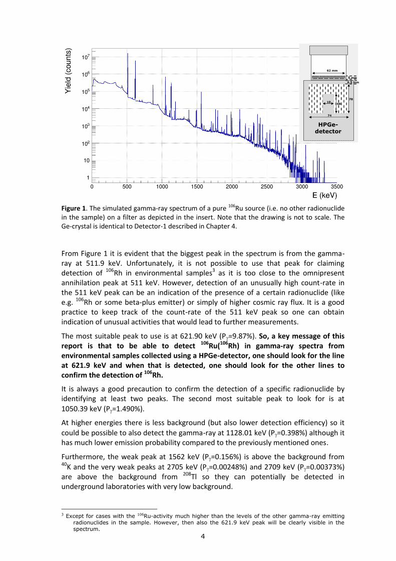
Figure 1. The simulated gamma-ray spectrum of a pure 106Ru source (i.e. no other radionuclide in the sample) on a filter as depicted in the insert. Note that the drawing is not to scale. The Ge-crystal is identical to Detector-1 described in Chapter 4.

From Figure 1 it is evident that the biggest peak in the spectrum is from the gamma-ray at 511.9 keV. Unfortunately, it is not possible to use that peak for claiming detection of 106Rh in environmental samples3 as it is too close to the omnipresent annihilation peak at 511 keV. However, detection of an unusually high count-rate in the 511 keV peak can be an indication of the presence of a certain radionuclide (like e.g. 106Rh or some beta-plus emitter) or simply of higher cosmic ray flux. It is a good practice to keep track of the count-rate of the 511 keV peak so one can obtain indication of unusual activities that would lead to further measurements.

The most suitable peak to use is at 621.90 keV (P=9.87%). So, a key message of this report is that to be able to detect 106Ru(106Rh) in gamma-ray spectra from environmental samples collected using a HPGe-detector, one should look for the line at 621.9 keV and when that is detected, one should look for the other lines to confirm the detection of 106Rh.

It is always a good precaution to confirm the detection of a specific radionuclide by identifying at least two peaks. The second most suitable peak to look for is at

1050.39 keV (P=1.490%).

At higher energies there is less background (but also lower detection efficiency) so it

could be possible to also detect the gamma-ray at 1128.01 keV (P=0.398%) although it has much lower emission probability compared to the previously mentioned ones.

Furthermore, the weak peak at 1562 keV (P=0.156%) is above the background from 40K and the very weak peaks at 2705 keV (P=0.00248%) and 2709 keV (P=0.00373%) are above the background from 208Tl so they can potentially be detected in underground laboratories with very low background.

3 Except for cases with the 106Ru-activity much higher than the levels of the other gamma-ray emitting

radionuclides in the sample. However, then also the 621.9 keV peak will be clearly visible in the spectrum.

5 mm

HPGe-detector

62 mm

74

78

6810

6.5 mm

5

3 Possible interferences

This list only contains "realistic" cases and thus not radionuclides with very short half-life, gamma-rays with very low emission probability or radionuclides with low likelihood to be present. For more thorough searches one can e.g. use the Nucléide-Lara tool: http://www.nucleide.org/Laraweb/ 511.9 keV: The omnipresent annihilation peak at 511 keV. Note that the annihilation peak is wider the other gamma-ray peaks due to Doppler broadening.

621.9 keV: 134I (621.79 keV); 110mAg (620.36 keV); 132I (621.2 keV and 620.9 keV);

154Eu (620.52 keV); 99Mo (620.03 keV and 621.77 keV); 126mSb (620.0 keV); 126Sb (620.1

keV); 228Ac (620.32 keV and 623.48 keV).

1050.4 keV: 72Ga (1050.69 keV); 150Eu (1049.04 keV); 214Bi (1051.96 keV);

134I (1052.2 keV); 132I (1049.6 keV); 154Eu (1049.4 keV); 110mAg (1050.5 keV).

1128.0 keV: 26Al (1129.67 keV); 96Nb (1126.96 keV); 154Eu (1128.55 keV); 234Pa (1126.8 keV); 132I (1126.5 keV); 214Bi (1130.29 keV).

1562 keV: 56Ni (1561.8 keV); 110mAg (1562.3 keV); 228Ac (1560.02 keV).

4 Coincidence summing correction factors

To evaluate qualitatively, which combination of different gamma-rays that are produced in a single decay it is useful to study the decay scheme of 106Rh which can been seen at http://www.nucleide.org/DDEP_WG/Nuclides/Rh-106_tables.pdf. Using the EGSnrc Monte Carlo code, coincidence summing correction factors were calculated (Lutter et al., 2017) for eight cases as shown in Tables 1 and 2. The numbers are given without uncertainty as they are intended as guidance of the magnitude of the correction and the exact values are only valid for the specific case for which they are calculated. By comparing a given sample/detector combination with the data in Tables 1 and 2 it is possible to make inter/extrapolation to come up with rough values, which should be a better approach compared to neglecting the effect (Sima, 1996), (Sima and Arnold, 2012). However, an uncertainty has to be attributed to this parameter should it be used in a calculation of activity. It is up to the user to investigate what a suitable uncertainty is for their specific detection system (Lépy et al., 2015).

The following configuration was used for the data in Tables 1 and 2: Sample: organic material (maize powder) with density 0.751 g·cm-3

Container-1: polycarbonate container of cylindrical shape. Inner radius: 31 mm, wall thickness: 1.6 mm, bottom thickness: 1.5 mm. Filling height: 0.5 mm, 5 mm and 43 mm, air-gap of 3 mm between detector endcap and bottom of container.

6

Container-2: polycarbonate container of cylindrical shape. Inner radius: 62 mm, wall thickness: 1.6 mm, bottom thickness: 1.5 mm. Filling height: 86 mm, air-gap of 3 mm between detector endcap and bottom of container

Distance from top of endcap to bottom of container: 0 mm (i.e. sample directly on endcap)

Detector-1: Coaxial crystal with a relative efficiency of 90%, top deadlayer thickness 0.8 μm, side-deadlayer thickness 1.5 mm. Endcap made of aluminium with a thickness of 1 mm, distance from top of crystal to window: 6.5 mm.

Detector-2: Coaxial crystal with a relative efficiency of 20%, top deadlayer thickness 0.75 mm, side-deadlayer thickness 0.75 mm. Endcap made of aluminium with a thickness of 0.8 mm, distance from top of crystal to window: 7.0 mm.

Some key points to note when inter/extrapolating in Tables 1 and 2 and comparing with another system is that the effect of coincidence summing:

Increases with the size of the detector

Increases if the sample is closer to the detector

As a consequence of the previous point, the effect is bigger for small, thin samples compared to big samples

In Tables 1 and 2, a CF (efficiency Correction Factor) less than 1 means that counts are lost from the FEP (Full Energy Peak) by summing (summing-out) and consequently the effective efficiency is lower than the non-corrected efficiency. Following the same reasoning, a CF bigger than 1 means that in addition to the counts from the single gamma-ray with that energy, there is a contribution from summing of two other gamma-rays (summing-in). Note that in literature there are different definitions of the correction factors.

7

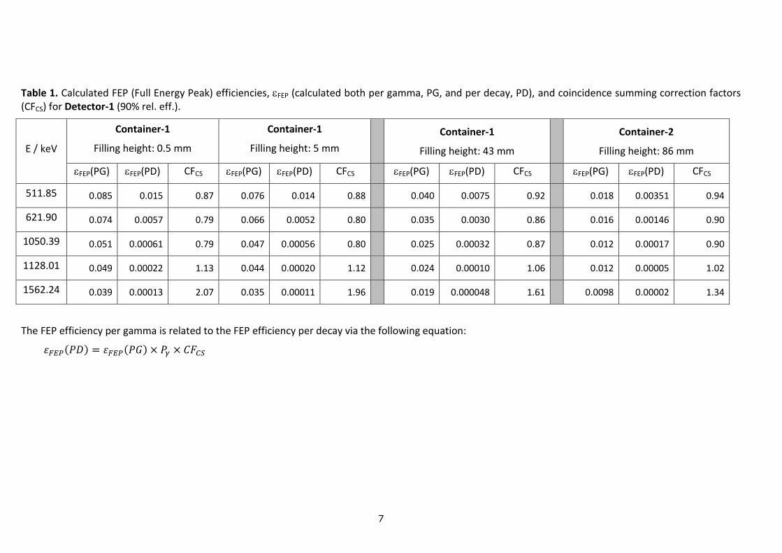
Table 1. Calculated FEP (Full Energy Peak) efficiencies, FEP (calculated both per gamma, PG, and per decay, PD), and coincidence summing correction factors (CFCS) for Detector-1 (90% rel. eff.).

E / keV

Container-1

Filling height: 0.5 mm

Container-1

Filling height: 5 mm

Container-1

Filling height: 43 mm

Container-2

Filling height: 86 mm

FEP(PG) FEP(PD) CFCS FEP(PG) FEP(PD) CFCS FEP(PG) FEP(PD) CFCS FEP(PG) FEP(PD) CFCS

511.85 0.085 0.015 0.87 0.076 0.014 0.88 0.040 0.0075 0.92 0.018 0.00351 0.94

621.90 0.074 0.0057 0.79 0.066 0.0052 0.80 0.035 0.0030 0.86 0.016 0.00146 0.90

1050.39 0.051 0.00061 0.79 0.047 0.00056 0.80 0.025 0.00032 0.87 0.012 0.00017 0.90

1128.01 0.049 0.00022 1.13 0.044 0.00020 1.12 0.024 0.00010 1.06 0.012 0.00005 1.02

1562.24 0.039 0.00013 2.07 0.035 0.00011 1.96 0.019 0.000048 1.61 0.0098 0.00002 1.34

The FEP efficiency per gamma is related to the FEP efficiency per decay via the following equation:

𝜀𝐹𝐸𝑃(𝑃𝐷) = 𝜀𝐹𝐸𝑃(𝑃𝐺) × 𝑃𝛾 × 𝐶𝐹𝐶𝑆

8

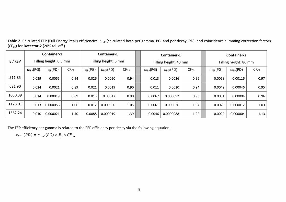
Table 2. Calculated FEP (Full Energy Peak) efficiencies, FEP (calculated both per gamma, PG, and per decay, PD), and coincidence summing correction factors (CFCS) for Detector-2 (20% rel. eff.).

E / keV

Container-1

Filling height: 0.5 mm

Container-1

Filling height: 5 mm

Container-1

Filling height: 43 mm

Container-2

Filling height: 86 mm

FEP(PG) FEP(PD) CFCS FEP(PG) FEP(PD) CFCS FEP(PG) FEP(PD) CFCS FEP(PG) FEP(PD) CFCS

511.85 0.029 0.0055 0.94 0.026 0.0050 0.94 0.013 0.0026 0.96 0.0058 0.00116 0.97

621.90 0.024 0.0021 0.89 0.021 0.0019 0.90 0.011 0.0010 0.94 0.0049 0.00046 0.95

1050.39 0.014 0.00019 0.89 0.013 0.00017 0.90 0.0067 0.000092 0.93 0.0031 0.00004 0.96

1128.01 0.013 0.000056 1.06 0.012 0.000050 1.05 0.0061 0.000026 1.04 0.0029 0.000012 1.03

1562.24 0.010 0.000021 1.40 0.0088 0.000019 1.39 0.0046 0.0000088 1.22 0.0022 0.000004 1.13

The FEP efficiency per gamma is related to the FEP efficiency per decay via the following equation:

𝜀𝐹𝐸𝑃(𝑃𝐷) = 𝜀𝐹𝐸𝑃(𝑃𝐺) × 𝑃𝛾 × 𝐶𝐹𝐶𝑆

9

One can note that the coincidence summing correction (CSC) increases with the size of the detector. Generally the CSC also increases when the sample size decreases. The sample with filling height 0.5 mm can be taken to mimic a filter and for that geometry the coincidence summing effect is bigger than for the sample with filling height 43 mm.

For the 621.9 keV line, one can note that for the thin sample on the big detector (Detector-1) the effect amounts to about 20% and for the small detector to about 10%.

Note that for the gamma-rays at 512, 622 and 1050 keV there is summing-out, i.e. pulses are lost from the full energy peak (FEP) and therefore the efficiency correction factor is less than unity. For the two lines of higher energy in Tables 1 and 2, there is summing-in and therefore the correction factor is higher than unity.

For the gamma-ray spectrometry practitioner it is positive to note that the emission probability for X-rays is very low and insignificant for applications involving environmental samples.

5 Angular correlation

The effect of angular correlation manifests itself in radionuclides with cascading gamma-rays, i.e. several gamma-rays that are emitted in one and the same (decay-) event. A well-known case with 100% correlation is the two 511 keV photons emitted following the annihilation of a positron. These two photons are emitted exactly at an angle of 180° from each other, which is made use of in e.g. PET (Positron Emission Tomography).

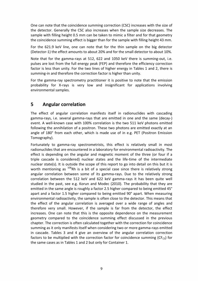
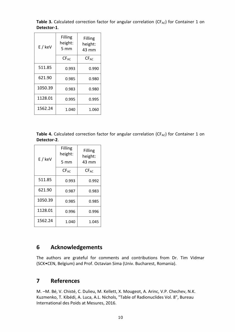
Fortunately to gamma-ray spectrometrists, this effect is relatively small in most radionuclides that are encountered in a laboratory for environmental radioactivity. The effect is depending on the angular and magnetic moment of the three (or four if a triple cascade is considered) nuclear states and the life-time of the intermediate nuclear state(s). It is outside the scope of this report to go into detail on this but it is worth mentioning as 106Rh is a bit of a special case since there is relatively strong angular correlation between some of its gamma-rays. Due to the relatively strong correlation between the 512 keV and 622 keV gamma-rays it has been quite well studied in the past, see e.g. Korun and Modec (2010). The probability that they are emitted in the same angle is roughly a factor 2.5 higher compared to being emitted 45° apart and a factor 1.5 higher compared to being emitted 90° apart. When measuring environmental radioactivity, the sample is often close to the detector. This means that the effect of the angular correlation is averaged over a wide range of angles and therefore very small. However, if the sample is far from the detector, the effect increases. One can note that this is the opposite dependence on the measurement geometry compared to the coincidence summing effect discussed in the previous chapter. The correction is often calculated together with the correction for coincidence summing as it only manifests itself when considering two or more gamma-rays emitted in cascade. Tables 3 and 4 give an overview of the angular correlation correction factors to be multiplied with the correction factor for coincidence summing (CFCS) for the same cases as in Tables 1 and 2 but only for Container 1.

10

Table 3. Calculated correction factor for angular correlation (CFAC) for Container 1 on Detector-1.

E / keV

Filling height: 5 mm

Filling height: 43 mm

CFAC CFAC

511.85 0.993 0.990

621.90 0.985 0.980

1050.39 0.983 0.980

1128.01 0.995 0.995

1562.24 1.040 1.060

Table 4. Calculated correction factor for angular correlation (CFAC) for Container 1 on Detector-2.

E / keV

Filling height:

5 mm

Filling height: 43 mm

CFAC CFAC

511.85 0.993 0.992

621.90 0.987 0.983

1050.39 0.985 0.985

1128.01 0.996 0.996

1562.24 1.040 1.045

6 Acknowledgements

The authors are grateful for comments and contributions from Dr. Tim Vidmar (SCK•CEN, Belgium) and Prof. Octavian Sima (Univ. Bucharest, Romania).

7 References

M. –M. Bé, V. Chisté, C. Dulieu, M. Kellett, X. Mougeot, A. Arinc, V.P. Chechev, N.K. Kuzmenko, T. Kibédi, A. Luca, A.L. Nichols, "Table of Radionuclides Vol. 8", Bureau International des Poids at Mesures, 2016.

11

K. Debertin, R. G. Helmer, "Gamma- and X-Ray Spectrometry with Semiconductor Detectors", North Holland, 1988. G. R. Gilmore, "Practical Gamma-ray Spectrometry, 2nd edition", John Wiley & Sons, Ltd, 2008. M.Korun, P. M. Modec, "Measurements of 106Ru activity in thin samples", Applied Radiation and Isotopes 68 pp 1392-1396, 2010. M. C. Lépy, A. Pearce and O. Sima, "Uncertainties in gamma-ray spectrometry", Metrologia 52 S123, 2015. G. Lutter, M. Hult, G. Marissens, H. Stroh, F. Tzika, “A gamma-ray spectrometry analysis software environment”, Applied Radiation and Isotopes, in Press. O. Sima, "Applications of Monte Carlo Calculations to Gamma-spectrometric Measurements of Environmental Samples", Applied Radiation and Isotopes 47, pp 919-923, 1996. O. Sima, D. Arnold, "Precise measurement and calculation of coincidence summing corrections for point and linear sources", Applied Radiation and Isotopes 70, pp 2107-2111, 2012.

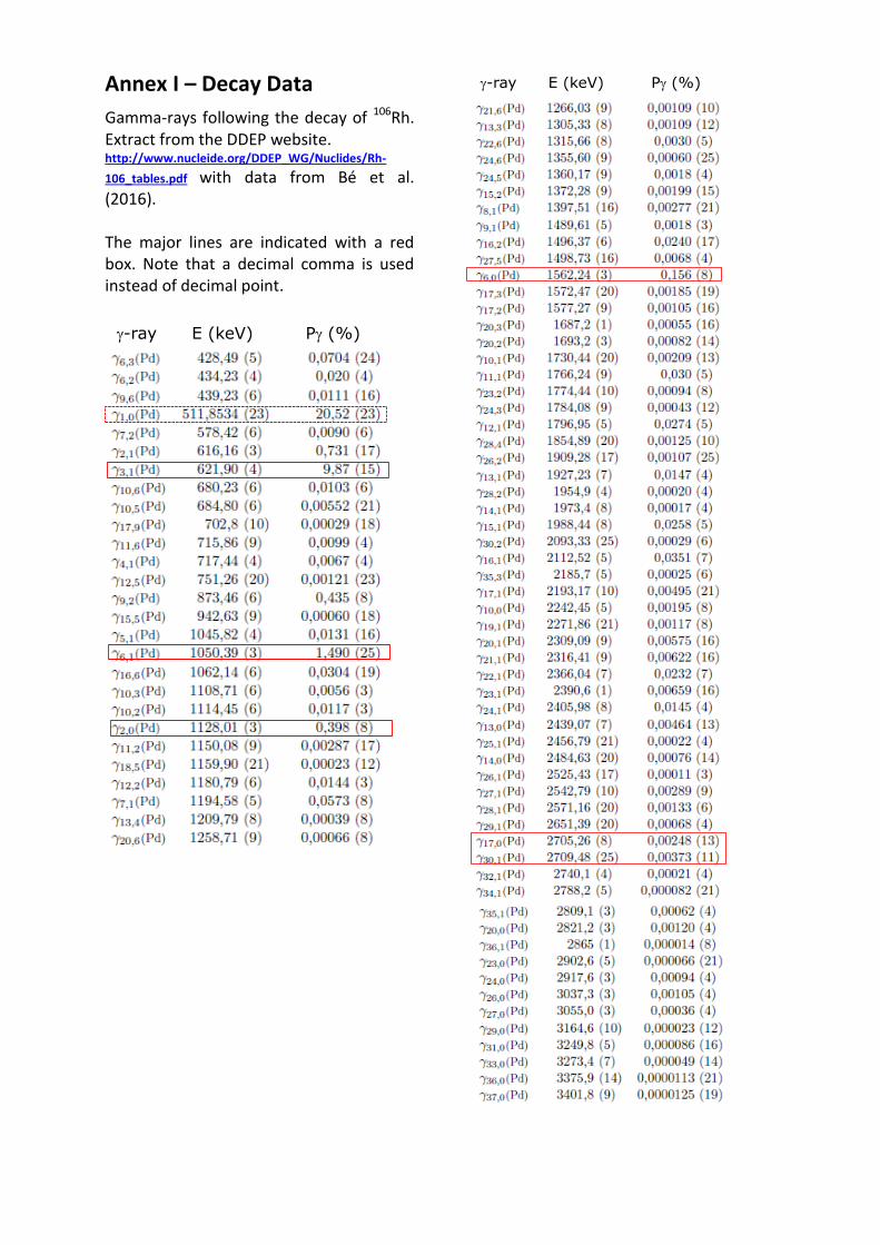
Annex I – Decay Data

Gamma-rays following the decay of 106Rh. Extract from the DDEP website. http://www.nucleide.org/DDEP_WG/Nuclides/Rh-

106_tables.pdf with data from Bé et al. (2016). The major lines are indicated with a red box. Note that a decimal comma is used instead of decimal point.

-ray E (keV) P (%)

-ray E (keV) P (%)

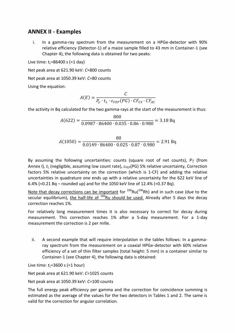
ANNEX II - Examples

i. In a gamma-ray spectrum from the measurement on a HPGe-detector with 90% relative efficiency (Detector-1) of a maize sample filled to 43 mm in Container-1 (see Chapter 4), the following data is obtained for two peaks:

Live time: tL=86400 s (=1 day)

Net peak area at 621.90 keV: C=800 counts

Net peak area at 1050.39 keV: C=80 counts

Using the equation:

𝐴(𝐸) =𝐶

𝑃𝛾 ∙ 𝑡𝐿 ∙ 𝜀𝐹𝐸𝑃(𝑃𝐺) ∙ 𝐶𝐹𝐶𝑆 ∙ 𝐶𝐹𝐴𝐶

the activity in Bq calculated for the two gamma-rays at the start of the measurement is thus:

𝐴(622) =800

0.0987 ∙ 86400 ∙ 0.035 ∙ 0.86 ∙ 0.980= 3.18 Bq

𝐴(1050) =80

0.0149 ∙ 86400 ∙ 0.025 ∙ 0.87 ∙ 0.980= 2.91 Bq

By assuming the following uncertainties: counts (square root of net counts), P (from

Annex I), tL (negligible, assuming low count rate), FEP(PG) 5% relative uncertainty, Correction factors 5% relative uncertainty on the correction (which is 1-CF) and adding the relative uncertainties in quadrature one ends up with a relative uncertainty for the 622 keV line of 6.4% (=0.21 Bq – rounded up) and for the 1050 keV line of 12.4% (=0.37 Bq).

Note that decay corrections can be important for 106Ru(106Rh) and in such case (due to the secular equilibrium), the half-life of 106Ru should be used. Already after 5 days the decay correction reaches 1%.

For relatively long measurement times it is also necessary to correct for decay during measurement. This correction reaches 1% after a 5-day measurement. For a 1-day measurement the correction is 2 per mille.

ii. A second example that will require interpolation in the tables follows: In a gamma-ray spectrum from the measurement on a coaxial HPGe-detector with 60% relative efficiency of a set of thin filter samples (total height: 5 mm) in a container similar to Container-1 (see Chapter 4), the following data is obtained:

Live time: tL=3600 s (=1 hour)

Net peak area at 621.90 keV: C=1025 counts

Net peak area at 1050.39 keV: C=100 counts

The full energy peak efficiency per gamma and the correction for coincidence summing is estimated as the average of the values for the two detectors in Tables 1 and 2. The same is valid for the correction for angular correlation.

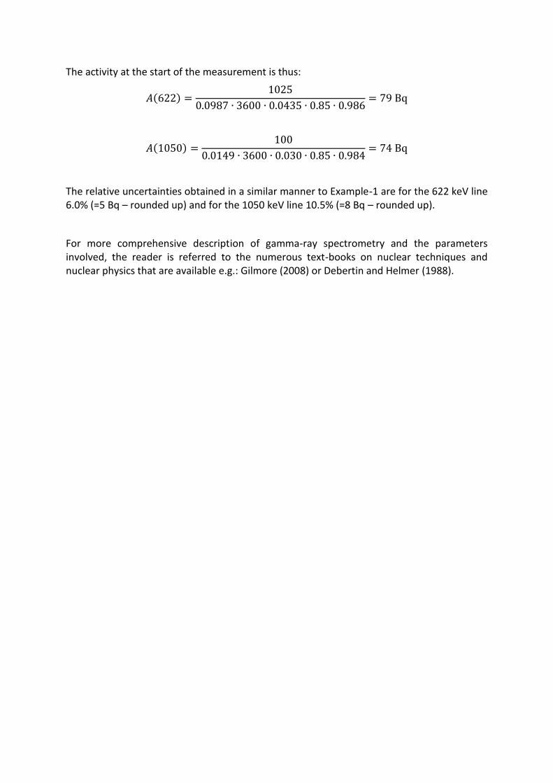
The activity at the start of the measurement is thus:

𝐴(622) =1025

0.0987 ∙ 3600 ∙ 0.0435 ∙ 0.85 ∙ 0.986= 79 Bq

𝐴(1050) =100

0.0149 ∙ 3600 ∙ 0.030 ∙ 0.85 ∙ 0.984= 74 Bq

The relative uncertainties obtained in a similar manner to Example-1 are for the 622 keV line 6.0% (=5 Bq – rounded up) and for the 1050 keV line 10.5% (=8 Bq – rounded up).

For more comprehensive description of gamma-ray spectrometry and the parameters involved, the reader is referred to the numerous text-books on nuclear techniques and nuclear physics that are available e.g.: Gilmore (2008) or Debertin and Helmer (1988).

GETTING IN TOUCH WITH THE EU

In person

All over the European Union there are hundreds of Europe Direct information centres. You can find the address of the centre nearest you at: http://europea.eu/contact

On the phone or by email

Europe Direct is a service that answers your questions about the European Union. You can contact this service:

- by freephone: 00 800 6 7 8 9 10 11 (certain operators may charge for these calls),

- at the following standard number: +32 22999696, or

- by electronic mail via: http://europa.eu/contact

FINDING INFORMATION ABOUT THE EU

Online

Information about the European Union in all the official languages of the EU is available on the Europa website at: http://europa.eu

EU publications You can download or order free and priced EU publications from EU Bookshop at:

http://bookshop.europa.eu. Multiple copies of free publications may be obtained by contacting Europe

Direct or your local information centre (see http://europa.eu/contact).

KJ-N

A-2

8850-E

N-N

doi:10.2760/62038

ISBN 978-92-79-74675-8