Detection and Spatial Delineation of Thin-Sand Sedimentary ... · evidenced in seismic-amplitude sections. Fig. 3 is a seismic cross section displaying high-angle clino-forms. Dip

246 April 2010 SPE Reservoir Evaluation & Engineering

Detection and Spatial Delineation of Thin-Sand Sedimentary Sequences With Joint Stochastic Inversion of

Well Logs and 3D Prestack Seismic Amplitude Data

Germán D. Merletti* and Carlos Torres-Verdín, The University of Texas at Austin

* Now with BP Americas.

Copyright © 2010 Society of Petroleum Engineers

This paper (SPE 102444) was accepted for presentation at the SPE Annual Technical Conference and Exhibition, San Antonio, Texas, USA, 24–27 September 2006, and revised for publication. Original manuscript received for review 30 June 2006. Revised manuscript received for review 9 January 2009. Paper peer approved 29 July 2009.

SummaryWe describe the successful application of a new prestack stochastic inversion algorithm to the spatial delineation of thin reservoir units otherwise poorly defined with deterministic inversion procedures. The inversion algorithm effectively combines the high vertical resolution of wireline logs with the relatively dense horizontal coverage of 3D prestack seismic amplitude data. Multiple partial-angle stacks of seismic amplitude data provide the degrees of freedom necessary to estimate spatial distributions of lithotype and compressional-wave (P-wave) and shear-wave (S-wave) velocities in a high-resolution stratigraphic/sedimentary grid. In turn, the estimated volumes of P- and S-wave velocity permit the statistical cosimulation of lithotype-dependent spatial distributions of poros-ity and permeability.

The new stochastic inversion algorithm maximizes a Bayesian selection criterion to populate values of lithotype and P- and S-wave velocities in the 3D simulation grid between wells. Property values are accepted by the Bayesian selection criterion only when they increase the statistical correlation between the simulated and recorded seismic amplitudes of all partial-angle stacks. Further-more, inversion results are conditioned by the predefined measures of spatial correlation (variograms) of the unknown properties, their statistical cross correlation, and the assumed global lithotype proportions.

Using field data acquired in a fluvial-deltaic sedimentary-rock sequence, we show that deterministic prestack seismic-inversion techniques fail to delineate thin reservoir units (10–15 m) pen-etrated by wells because of insufficient vertical resolution and low contrast of elastic properties. By comparison, the new stochastic inversion yields spatial distributions of lithotype and elastic prop-erties with a vertical resolution between 10–15 m that accurately describe spatial trends of clinoform sedimentary sequences and their associated reservoir units.

Blind-well tests and cross validation of inversion results con-firm the reliability of the estimated distributions of lithotype and P- and S-wave velocities. Inversion results provide new insight to the spatial and petrophysical character of existing flow units and enable the efficient planning of primary and secondary hydrocar-bon recovery operations.

Introduction 3D seismic amplitude data are commonly used to identify hydro-carbon reservoirs and to assess their spatial continuity. Modern seismic processing techniques enable the interpretation of time-migrated common-midpoint (CMP) gathers in terms of amplitude-vs.-offset (AVO) variations to estimate subsurface petrophysical

properties (Castagna and Backus 1993). More sophisticated appli-cations consist of directly determining spatial distributions of rock properties that best reproduce recorded seismic amplitudes (Sheriff and Geldart 1982). These procedures make use of seismic inver-sion algorithms implemented in fully or partially stacked normal-moveout (NMO) corrected gathers. The latter approach, referred to in this paper as prestack inversion, attempts to capture enhanced degrees of freedom in the measurements to yield independent estimates of density and P- and S-wave velocities (Contreras and Torres-Verdín 2005), which can be used to estimate lithology-dependent petrophysical properties (Goodway et al. 1997).

Despite the fact that many variants of seismic inversion proce-dures have been reported in the open technical literature, in this paper we classify them into two main categories: deterministic and stochastic methods. Geoscientists commonly use determin-istic inversion methods in their first attempt to interpret seismic amplitude reflection data in terms of quantitative rock properties. To accomplish this, deterministic inversion algorithms minimize an objective function that contains at least two additive terms (Debeye and van Riel 1990; Pendrel 2001): One of these terms controls the misfit between recorded and synthetic seismic amplitudes, and a second term controls the energy of the inverted reflectivities. The inversion includes a stabilization factor that places a differential weight between the metric of data misfit and the energy of the inverted reflectivities. Practical applications of prestack inversion indicate that S-wave velocity and bulk density are more difficult to estimate than P-wave velocity. Consequently, additional terms are often included in the objective function to enforce soft nonlin-ear relationships between elastic properties (Fowler et al. 2000). Deterministic inversion procedures do not honor well logs in a direct manner, and, hence, the frequency bandwidth of the inverted products is the same as that of the recorded seismic amplitudes.

Stochastic (or geostatistical) inversion techniques, on the other hand, use a completely different approach to estimate elastic and/or petrophysical properties (Pendrel 2001). In their simplest form, stochastic inversion methods consist of two sequential procedures: The first one populates the interwell space with rock properties. This interpolation is performed in a 3D stratigraphic/structural simulation grid with time sampling interval two- or four-fold the original sampling interval of the recorded seismic amplitudes. Subsequently, interpolated samples are entered into an algorithm that numerically simulates seismic amplitudes to quantify the corresponding data misfit (Haas and Dubrule 1994). The stochas-tic inversion algorithm will accept or reject the geostatistically simulated property values depending on their agreement with the recorded seismic amplitudes.

Because they explicitly combine well logs and seismic amplitude variations, stochastic inversion procedures are particularly useful to detect and delineate thin reservoirs otherwise poorly defined by deterministic inversion techniques. In this paper, we refer to as “thin reservoir” one whose thickness is below the vertical resolution of the available seismic amplitude data. Some authors have success-fully implemented post-stack stochastic inversion techniques to improve the detection and spatial delineation of individual fluvial

April 2010 SPE Reservoir Evaluation & Engineering 247

hydrocarbon reservoirs within amalgamated sandstone complexes (Torres-Verdín et al. 1999; Merletti et al. 2003).

The objective of this paper is to describe the successful imple-mentation of a new prestack stochastic inversion algorithm recently developed by Fugro-Jason. The inversion algorithm effectively combines the high vertical resolution of well logs with the dense horizontally coverage of seismic amplitude data. We integrate these two complementary measurements with a stratigraphic geological model constructed with quantitative knowledge of reservoir archi-tecture. Inverted products exhibit a vertical resolution intermediate between the vertical resolution of well logs and seismic amplitude data. The relative increase of vertical resolution, compared to that of seismic amplitude data, improves the interpretation of complex delta progradations (clinoform geometries) of the fluvial-deltaic sedimentary rock sequences. In addition, we make use of analog synthetic reservoir models constructed with the edited logs to verify the reliability and vertical resolution of inverted products under controlled conditions of seismic data quality, well proximity, and number of wells.

Previously documented experience with prestack stochastic inversion considered the spatial delineation of relatively thick sedimentary units, as well as the estimation of their porosity, per-meability, and water saturation (Contreras et al. 2005; Contreras et al. 2006). However, in this paper we describe the first applica-tion of prestack stochastic inversion to the delineation of laterally varying thinly bedded reservoirs.

In the following sections, we first introduce the data set used to implement the stochastic inversion procedure. Secondly, we describe the method used to approach the petrophysical evaluation of wireline logs. We perform deterministic inversion to verify its limitations in detecting reservoir-scale heterogeneities. Subse-quently, we describe the new stochastic inversion as implemented with three partial-angle stacks. Later, and after applying rigorous quality control to the inverted elastic properties, we cosimulate petrophysical properties statistically related to elastic properties. We further appraise determinist and stochastic inversion products with analog synthetic reservoir models and noise-free numerically simulated seismic amplitude data. Finally, we discuss relevant observations concerning the interpretation of inversion results and summarize our conclusions.

Data Set and Local Geology. The data set used for the study reported in this paper was acquired in an active hydrocarbon fi eld located in Venezuela’s Barinas-Apure basin. Fig. 1 shows an approximately 6.5×5.5-km2 subset of the 14.2×25.4-km2 seismic data used to implement the stochastic inversion procedure. The seismic data were acquired with a time sampling interval of 4 ms and a square bin size of 75 m. Spectral analysis within the hydro-carbon-producing units indicates a frequency content between 5 and 65 Hz and a dominant frequency of 28 Hz. Wavelet extractions evidenced an average phase spectrum of 90°. For a value of P-wave velocity of 4500 m/s, we estimated a tuning wavelength of 30 m. This calculation indicates that the available seismic data do not enable the direct detection of individual hydrocarbon-producing units in the area.

The data subset includes three vertical and two deviated wells. Fig. 2 displays the well logs acquired in Well 37. Wireline mea-surements usually consist of gamma ray, resistivity, neutron, bulk-density, and P-sonic logs; S-wave sonic logs were available only in Well 37. Well logs comprise several depth intervals in which the measurements are strongly affected by washouts and borehole rugosity. We edited such intervals before computing petrophysical properties. Two seismic-time horizons were available throughout the entire seismic cube. These horizons coincide with the tops of the two main hydrocarbon-producing units of the basin. For simplicity, we refer to these formation units as Formation E and Formation C.

Formation E is a 25- to 35-m-thick mixed carbonate and silici-clastic interval composed of limestone, dolostone, arenitic dolos-tone, and calcareous sandstone intercalated with shales and calcare-ous shales. Fig. 2 describes the location of Formation E in the depth range of 10,700–10,800 ft. The depositional environment interpreted for this formation is a shallow marine carbonate platform with vari-able periods of exposure (Aquino et al. 1997). On the other hand, Formation C, which is the target of our studies, is a 250- to 300 ft-thick medium- to coarse-grained sandstone (Fig. 2) with slight amounts of shale. The base of this formation is interpreted as depos-ited by large bedload-dominated braided rivers filling incised valleys (Bejarano 2000). Such deposits were transgressed and overlain by an extensive sheet of shoreface and braided delta sediments (center Formation C). There were some episodes in which the rate of sedi-mentation was greater than the rate of accommodation (Bejarano

Fig. 1—Seismic-time horizon displaying the embedding geological structure and the location of vertical and deviated wells. The right-hand side panel is an enlarged view of the 6.5×5.5 km2 seismic data subset used to implement stochastic inversion.


2000). This explains the extensive progradational stacking patterns displayed in wireline logs and prograding clinoform geometries evidenced in seismic-amplitude sections.

Fig. 3 is a seismic cross section displaying high-angle clino-forms. Dip angles of 4–5° measured at well locations outside the study area support the interpretation of fluvial-dominated deltaic deposits rather than shoreface deposits (Walker and Plint 1992).

Fig. 3 also displays an enlarged view of typical well-log responses. The gamma ray log (shown in green) does not evidence important lithology variations through the interval, whereas the log-derived porosity (shown in yellow) does display grain-size trends with better reservoir conditions toward the top. Either one or two upward-coarsening units are found in the interval represented by deltaic deposits; these trends are interpreted as the advance of

Fig. 2—Wireline logs acquired in Well 37. The far-right panel describes the lithology proportions (sandstone in yellow, carbon-ate in red, and shale in dark grey) and porosity (cyan). The depth interval of interest considered in this paper corresponds to Formation C (9,800–10,200 ft).

Fig. 3—Seismic cross section displaying some prograding clinoforms within Formation C. For reference, the gamma ray and computed-porosity logs are posted along the trajectory of Well 55.


delta-front sands over prodelta and platform muds (Galloway and Hobday 1990). Fluvial deposits are also found in the upper sec-tion and are overlain by thin bioclastic carbonates, referred in this paper to as Formation B. Given the small thickness of the basal fluvial deposits and the strong seismic interference produced by carbonates in the upper Formation C, we focus our efforts on improving the spatial delineation of deltaic deposits in areas in which clinoform configurations are poorly defined or not defined at all. The average thickness of individual reservoirs is 10–15 m, although in some cases reservoir units appear as amalgamated lay-ers whose thickness is close to the vertical resolution of seismic amplitude data (30 m). Both the high degree of compaction of reservoir units and the absence of thicker shaly intervals between them make it very difficult to delineate individual reservoir units with conventional seismic interpretation techniques.

Petrophysical Analysis. We synthesized volume-of-shale, poros-ity, water saturation, and permeability logs using standard petro-physical evaluation techniques. Volumetric shale concentration (Csh) was calculated using a linear shale index (Ish) (Dewan 1983). Second, we computed porosity from the density log using a quartz-mineral matrix and a single-fl uid (brine) model. Given that neither abundant shaliness nor gas is found within producing reservoirs, an arithmetic average of shale-corrected neutron and density porosities is a good approximation of nonshale porosity. We simultaneously computed water saturation and fl uid-corrected porosity using Archie’s model with an iterative minimization procedure that corrected the error introduced by the assumption of brine saturation during the previous estimation of porosity. Calculation of irreducible water saturation logs was the fi rst step in computing permeability. We then used linear multivariate regression with well-log-derived porosity and irreducible water saturation to estimate permeability. Fig. 4 shows a good agreement between core- and log-derived permeabilities within hydrocarbon producing units.

Fluid/Lithology Sensitivity Analysis. Three independent exer-cises were performed to determine the sensitivity of elastic proper-ties to variations of lithology, porosity, and pore fl uid. We applied these techniques in the following order: (1) numerical simulation of synthetic seismic gathers (together with analysis of recorded seismic gathers), (2) Biot-Gassmann fl uid substitution, and (3) crossplot analysis. Before the application of these techniques, we reconstructed several synthetic S-wave velocity logs because the original data set included only one measured log. Log reconstruc-tion included: (1) estimation of elastic constants (bulk and shear moduli) for dry rock given initial values of P-wave velocity, porosity, and water saturation (Hilterman 1983) and (2) calcula-tion of S-wave velocity using the estimated shear modulus and the measured bulk density.

First, we simulated NMO corrected synthetic gathers using well logs. Synthetic gathers are the result of the convolution of a previ-ously estimated wavelet with well-log angle-dependent reflectivi-ties. Reflectivities were computed by means of Knott-Zoeppritz equations (Aki and Richards 1980) using recorded and synthetic P- and S-wave velocities, and density logs. The simulated seismic amplitude gathers are displayed in Fig. 5a, and the measured gathers in Fig. 5b. Differences between simulated and measured amplitudes can be attributed to the way in which amplitudes were generated. Specifically, simulated gathers were computed from log-derived elastic properties, which are representative of a volume of investigation a few inches from the borehole wall. On the other hand, measured gathers represent the average of much larger rock volumes of sensitivity. Both synthetic and recorded seismic gath-ers exhibit a monotonic decrease of amplitude with an increase of angle of incidence. This behavior corresponds to the classic AVO response of Class-I sands (Rutherford and Williams 1989), which is typical of sediments that underwent a gradual burial history. Secondly, we performed fluid-substitution analysis to determine the influence of pore-fluid saturation on P- and S-wave velocities. In so doing, we applied Biot-Gassmann’s equations assuming a

Fig. 4—Results from standard petrophysical evaluation of wireline logs acquired in Well 67. There is a good agreement between the available rock-core data and well-log-derived porosity and permeability.


constant porosity of 20% (this is the largest value of porosity computed from well logs). Fig. 6 shows that P-wave velocity (red curve) is nearly insensitive to mixtures of oil and water filling the pore space; this figure also displays the P-wave velocity for the case of gas saturation instead of liquid hydrocarbon saturation (green curve). The analysis indicates that S-wave velocity (blue curve) does not change appreciably over the entire range of fluid saturation. As predicted by Biot-Gassmann’s equations applied to consolidated sediments, both rigidity and bulk moduli increase with compaction, thereby minimizing the effect of fluid saturation on the measured rock velocities (Tatham et al. 1991).

Crossplot analysis of well log-derived elastic properties (P- and S-wave velocities, and density) and petrophysical properties (porosity and permeability) shows that the cleanest sandstones are associated with values of P- and S-wave velocity smaller than 4300 and 2600 m/s, respectively (Fig. 7). On the other hand, high values of elastic properties are associated with sandstones containing larger volumes of fine materials or smaller grain sizes. In addition, we computed the fluid- and lithology-sensitive Lamè petrophysi-cal parameters, LambdaRho and MuRho (Goodway et al. 1997). Values of MuRho below 30 GPa·g/cm3 indicate good-quality rocks (Fig. 8). Fig. 9 displays the crossplot of these parameters. As

(a) (b) (c)

Fig. 5—Synthetic (a) and recorded (b) angle gathers in Well 84 exhibit a decrease of amplitude with an increase of angle of incidence (typical behavior of Class-I reservoirs). Synthetic angle gathers were computed using angle-dependent reflectivities and extracted wavelets. For reference, Fig. 5c shows the measured P-wave velocity log.

Vp modeledVs modeledVp gasVp wellsVs wells

Fig. 6—Biot-Gassmann fluid substitution indicates that P-wave velocity (red curve) does not change significantly with an increase of oil saturation. There is a larger variation of P-wave velocity for the hypothetical case of gas saturating the pore space (green curve), but this occurrence has not been reported in the study area. S-wave velocity (blue curve) remains almost constant with changes of oil/water ratio. Numbered symbols identify average P- and S-wave velocities (red and blue, respectively) selected from well-log readings of 20% porosity.


expected, MuRho is an excellent discriminator of facies, whereas LambdaRho shows the same dynamic range for all the facies. Such behavior supported our previous observations stemming from the Biot-Gassmann behavior of oil/water mixtures: Elastic parameters remain almost insensitive to variations of oil/water saturation.

Because of the lack of sensitivity of elastic parameters to variations of oil/water saturation, in what follows we focus our attention only on estimating spatial distributions of porosity and permeability from inverted elastic properties. Crossplot and histo-gram analysis indicated that P- and S-wave velocities exhibited a

shaly sands

clean sands

Fig. 7—Crossplot of P- and S-wave velocities constructed with wireline logs acquired in Well 37. The color code identifies the corresponding value of porosity. Porous sands exhibit low values of P- and S-wave velocity, whereas shaly sands are associated with high values of P- and S-wave velocity. Histograms evidence the existence of two distinct populations of samples clearly differentiated by P- and S-wave velocities.

shaly sands

clean sands

Fig. 8—Crossplot of Vp /Vs ratio and density constructed with wireline logs acquired in Well 37. The color code identifies the corresponding value of porosity. Density is an excellent discriminator of porous and shaly sands whereas the Vp /Vs ratio is not because the two sand groups are associated with the same dynamic range (1.55–1.75).


bimodal distribution of samples corresponding to an equal num-ber of lithotypes: (1) clean sands, including porous and perme-able intervals, and (2) shaly sands, including finely grained and shale-laminated sands. Such an approach for the differentiation of lithotype based on the combined use of P- and S-wave velocities is attractive because it permits the determination of lithotype from seismic inversion products.

Deterministic Inversion. NMO-corrected partial-angle stacks were entered to inversion on the basis of comparisons between syn-thetic (numerically simulated) and recorded angle gathers. Angu-lar ranges were available from seismic amplitude data between 5 and 25°. For the study described in this paper, we chose the following angle ranges: 5–14°, 10–19°, and 16–25°. In an effort to improve signal-to-noise ratios, a small overlap between angle ranges was included in the separation of angle ranges, given the limited number of traces available for stacking. Angle-dependent wavelets were estimated for each partial-angle stack in two steps: (a) calculation of angle-dependent refl ectivities (for the angle ranges listed above) using density and P- and S-wave velocity logs and (b) wavelet estimation by minimizing the least-squares difference between simulated and recorded partial-angle stacks in the vicinity of wells.

The deterministic inversion used in this paper is an algorithm developed by Fugro-Jason as an extension to nonzero offsets of their constrained sparse-spike inversion (CSSI) (Debeye and van Riel 1990). This algorithm minimizes an objective function that combines the L1-norm of reflectivity series and the L2-norm of the seismic misfit (expressed as the difference between simulated and recorded seismic amplitudes). The interplay of these two additive terms in the inversion is adjusted with a stabilization factor (or Lagrange multiplier). A third additive term uses the L1-norm met-ric to bias low-frequency components of inverted products toward low-frequency models constructed with the interpolation of well logs. We emphasize that, for the deterministic inversion exercises described in this paper, we did not enforce an explicit relationship between density and P- and S-wave velocities. Likewise, we did

not enforce value-range constraints when minimizing the objec-tive function.

Fig. 10 is a three-panel seismic-time cross section that shows the deterministically inverted volumes of P-wave and S-wave impedances (impedance being the product of velocity and density) and density, together with the gamma ray and computed porosity logs posted along two well trajectories. Despite the low seismic residuals yielded by the inversion (low data misfit), the computed porosity log clearly indicates that inverted parameters are unable to reproduce reservoir-scale heterogeneities. From direct comparison of well logs and inverted products along well trajectories, we found that the vertical resolution of deterministically inverted volumes of P- and S-wave impedance was approximately 25 m. As noted earlier, the relatively high degree of compaction of reservoir units causes a small contrast of elastic properties between reservoir units and their embedding rocks, and this makes it very difficult to delineate individual reservoir units from deterministically inverted elastic properties.

Stochastic Inversion. In most cases, low vertical resolution of seismic amplitude data is the main motivation for implementing stochastic inversion procedures. However, in this paper, the choice of stochastic inversion is equally motivated by the geometrical properties of the reservoir units under consideration. Specifi cally, and as noted in Fig. 3, there are several reservoir sections in which clinoform geometries are well defi ned by seismic amplitude data (left-hand side of the section), whereas there are other places where such geometries are poorly defi ned, whereby their existence had to be corroborated with wireline logs and well-derived petrophysical logs (right-hand side of the section). The integration of seismic amplitude data, well logs, and geological knowledge of reservoir architecture allowed us to construct a high-resolution stratigraphic/structural property volume with one-fourth of the original time sampling rate of seismic amplitude data.

Given that not only low-frequency components of wireline logs are used by the stochastic inversion but also some of their high-fre-quency components, we performed a strict well-log quality control

shaly sands

clean sands

LambdaRho [GPa⋅g/cm3]

Fig. 9—Crossplot of LambdaRho and MuRho constructed with wireline logs acquired in Well 37. The color code identifies the corresponding value of porosity. Porous sands are associated with low values of MuRho; the vertical histogram indicates that this parameter is an excellent discriminator of rock quality. LambdaRho, in turn, does not differentiate petrophysical properties (all the samples fall within the range of 23 and 35 GPa·g/cm3).


to identify intervals during which wireline logs did not respond to formation properties. In those sections, we computed synthetic logs (P- and S-wave velocities and density) following three steps: (a) assessment of lithology fractions by means of multilinear regres-sion, (b) calculation of synthetic logs using the product of lithology fractions and theoretical readings for pure-mineral compositions, and (c) replacement of measured logs with synthetic logs at places where caliper readings exceeded 10% of the nominal bit size. Partial-angle stacks, angle-dependent wavelets, high-resolution (1 ms) stratigraphic/structural framework, lithotype (clean and shaly sands) logs, and corrected-by-caliper P- and S-wave velocities and density logs formed the input data set used for prestack stochastic inversion.

The stochastic inversion algorithm used in this paper is based on a Bayesian strategy with Markov-Chain Monte-Carlo (MCMC) updates (Gilks et al. 1996; Chen et al. 2000) to sample the poste-rior (model space) probability density function (PDF). Beginning with a prior PDF of the unknown model properties, the objective of Bayesian inversion is to sample the posterior PDF to find all possible model realizations that honor the measurements within the predefined signal-to-noise ratio. MCMC implements a biased random walk to sample the posterior PDF. The trajectory of the walk is modified continuously to target points in model space which honor the measurements and their uncertainties (Tarantola 2005). This procedure requires that a data likelihood function be evaluated at each step of the random walk; in other words, such a procedure requires the repeated solution of the forward problem. The numerical simulation consists of (a) computing angle-depen-dent reflectivities from the simulated values of elastic properties, (b) convolving angle-dependent wavelets with angle-dependent reflectivities to numerically simulate angle-dependent seismic traces, and (c) computing the metric of the difference (seismic

residual) between simulated and recorded seismic traces. The final point of the random walk is the location in model space in which the posterior PDF exhibits a local maximum.

In this project, a priori models (volumes of lithotype, P-wave velocity, S-wave velocity, and density) were constructed with sequential Gaussian simulation (SGS) (Chilès and Delfiner 1999) of well-log properties using predefined PDFs and assumed mea-sures of spatial correlation (variograms). We selected the variogram model and its properties (lateral and vertical ranges) with adher-ence to outcrop geological analogs. In addition, the construction of a priori models enforced predefined lithotype-dependent statistical cross-correlations (joint PDFs) between P-wave velocity, S-wave velocity, and density constructed with well logs. We estimated joint PDFs of elastic properties (density, and P- and S-wave velocities) based on two possibilities of lithotype: porous sands and shaly sands. Furthermore, simulations of lithotype were made to honor a predefined global measure of facies proportion.

Figs. 11 and 12 show samples of properties collected from well logs of “shaly sands” and “clean sands,” respectively, for the complete interval of interest; the same figures display projections over 2D Cartesian planes of 3D joint PDFs constructed with well-log data. Fig. 13 displays a 3D joint PDF of elastic properties confirming that each lithotype is associated with nonoverlapping 3D subdomains of elastic properties.

Fig. 14 compares the high vertical resolution of stochastically inverted P-wave velocity (lower panel) against the deterministi-cally inverted P-wave impedance (center panel) and the near partial-angle stack (upper panel). We note that both the expression of clinoform geometries and the P-wave velocity contrast between embedding rocks and reservoir units have been enhanced by the stochastic inversion when compared to those of deterministically inverted products. Fig. 15 shows seismic-time cross sections of the

[g/cm3⋅m/s]

[g/cm3⋅m/s]

[g/cm3]

(a)

(b)

(c)

Fig. 10—Seismic-time cross section showing the results of deterministic inversion of prestack seismic amplitude data: P-impedance, S-impedance, and density. The well-log-derived porosity (the curve posted on the right-hand side of each well track) indicates that inverted property volumes are unable to resolve reservoir-scale heterogeneities (some of these heterogeneities are indicated with white arrows).


stochastically inverted elastic properties (P- and S-wave velocities and density) in the 1-ms high-resolution stratigraphic framework. These figures confirm the increase of vertical resolution of sto-chastically inverted products compared to that of the corresponding deterministically inverted products. Such a result comes as a direct consequence of the combined quantitative use of well logs, 3D prestack seismic amplitude data, and the geological/stratigraphic framework.

Analysis of Results. We found that the stochastically inverted property distributions remained sensitive to some of the parameters used to construct a priori models and to parameters associated with the inversion process. To shed light on such dependence, we analyzed several combinations of inversion parameters to deter-mine their impact on the cross correlation between measured and synthetic seismic amplitudes. In this context, synthetic amplitudes correspond to seismic amplitudes numerically simulated from the elastic-property models yielded by the inversion. Inversion param-eters analyzed included: (1) assumed global lithotype proportions, (2) vertical and lateral ranges of the assumed variograms, (3) sig-nal-to-noise ratio of the seismic amplitude data, and (4) variogram type. Sensitivity analyses near available wells indicated that the fi rst two parameters listed above exerted the greatest infl uence on inversion results. We interpreted such dependence as caused by (1) the relatively low vertical resolution of the recorded seismic amplitudes or (2) the large degree of amalgamation of coarse deposits between successive clinoforms (possibly associated with a decrease in accommodation space). Any of these two adverse conditions can obscure the imprint of dipping layer boundaries on seismic amplitude data, thereby considerably increasing the

non-uniqueness of inversion results. We observed this behavior in the central and southern areas of the seismic data subset that, incidentally, included the location of the fi ve available wells.

The best inversion results were obtained with a priori models constructed with variogram vertical and lateral ranges of 6 ms and 900 m, respectively. Assumed lithotype proportions for such models were 30% for “clean sands” and 70% for “shaly sands.” Moreover, we found that the choice of variogram type did not exert relevant influence on inversion results. However, for normalization purposes, all the inversion examples described in this paper were implemented with exponential variograms.

Fig. 16 displays the normalized sum of quadratic differences between angle-dependent synthetic and recorded seismic data as cross-correlation maps. The cross correlation is greater than 95% in most places and decreases to 70% in the proximity of faults.

In addition to the appraisal of data fit (cross correlation), we performed blind-well tests to appraise the choice of inversion parameters. Fig. 17 shows the stochastically inverted density, and P- and S-wave velocities at the location of a well not included in the construction of the a priori model. The agreement between measured and stochastically inverted P- and S-wave velocities is remarkable (two first panels). Moreover, the vertical resolution gained is consistent with the variability of well-log measurements and helps to delineate the most important reservoir heterogene-ities. For instance, the thin bed located between 2075 and 2085 ms is successfully resolved by stochastic inversion (black curve), whereas the same reservoir feature is vertically averaged with shouldering beds by deterministic inversion (red smooth curve). For the case of density, the inverted distribution does not match the measured well-log density (far-right panel). We believe that

[g/cm3]

Fig. 11—Example of a 3D lithotype-dependent joint PDF of P-wave velocity, S-wave velocity, and density constructed with wireline logs acquired in Well 37. Green cubes identify well-log samples for “shaly sands” gathered from the entire interval of interest. Color-coded 2D Cartesian planes describe projections of the sampled 3D joint PDF, with the colors indicating relative concentration of samples.


Density[g/cm3]

Fig. 12—Example of a 3D lithotype-dependent joint PDF of P-wave velocity, S-wave velocity, and density, constructed with wireline logs acquired in Well 37. Red cubes identify well-log samples for “clean sands” gathered from the entire interval of interest. Color-coded 2D Cartesian planes describe projections of the sampled 3D joint PDF, with the colors indicating relative concentration of samples.

Density[g/cm3]

Fig. 13—3D joint PDF of P-wave velocity, S-wave velocity, and density constructed with wireline logs acquired in Well 37 and displaying the non-overlapping model space occupied by the two lithotypes: clean sands (red) and shaly sands (green).


the limited angular coverage available from the recorded seismic gathers (25°) does not allow the reliable and accurate estimation of density. Fig. 17 also compares the vertical resolution associated with deterministic and stochastic inversion products. On the basis of the comparison of the two results, we estimate the vertical reso-lution of stochastic inversion products to be approximately 10–15 m, whereas the resolution of deterministic inversion products is estimated to be 25–30 m. We emphasize that the difference in verti-cal resolution is because of the fact that the stochastic inversion enforces a tight connection between seismic amplitude data and well logs, whereas the deterministic inversion does not.

Cosimulation of Petrophysical Properties. A common procedure used to estimate petrophysical properties from inverted elastic properties is to establish a statistical correlation between one elas-tic property (for instance, P- or S-wave impedance) and one pet-rophysical property, such as porosity (Pendrel and van Riel 1997). Prestack stochastic inversion yields spatial distributions of density, and P- and S-wave velocities that, when properly cross validated, provide the degrees of freedom necessary to reliably cosimulate more than one petrophysical property. Our approach consists of constructing 3D joint PDFs of elastic and petrophysical properties; namely, we quantify the degree of statistical correlation between elastic and petrophysical properties with a lithotype-dependent joint multidimensional PDF. Such joint PDFs are constructed from lithotype-dependent well-log samples of elastic properties and well-log derived petrophysical properties. Figs. 18 and 19 show 3D joint PDFs between P- and S-wave velocities and porosity, and

between P- and S-wave velocities and permeability, respectively, for the lithotype “clean sands.” The same fi gures display the pro-jection over 2D Cartesian planes of the 3D joint PDFs constructed with well-log samples.

We cosimulated porosity and permeability from inverted elastic properties by constructing 3D joint PDFs of P-wave velocity, S-wave velocity, and each of these two petrophysical properties. In so doing, we decided not to include density in the cosimulations because the stochastically inverted distributions of this property did not agree with measured density logs at blind-well locations (Fig. 17). The final petrophysical volumes were obtained by averaging 30 independent cosimulations of porosity and permeability.

After performing the cosimulation, we mapped eight porous and permeable units within the area of study, all of which exhibited a north-northeast/south-southwest strike. Fig. 20 shows one such reservoir unit, 1500–2000 m long and less than 1000 m wide; it also describes the spatial distribution of the cosimulated porosity within the reservoir unit.

Generation and Inversion of Analog Synthetic Reservoir Models. One of the central objectives of our study was to quantify the accuracy and reliability of the new stochastic inversion algorithm to delineate thin, dipping reservoir geometries. As emphasized in previous sections, there are not well-defi ned clinoform structures at existing borehole locations. On the other hand, clinoform geom-etries are evidenced in the northern areas of the study that, coinci-dentally, are currently devoid of wells. In order to assess the ability of prestack seismic amplitude data to detect and spatially delineate

[g/cm3⋅m/s]

(a)

(b)

(c)

Fig. 14—Seismic-time cross section emphasizing the enhancement of vertical resolution of the P-wave velocity volume (c) derived from the stochastic inversion of prestack seismic amplitude data, (a) near partial-angle seismic stack, and (b) deterministically inverted P-wave impedance panels are included for comparison.


(a)

(b)

(c)

Density, g/cm3

Fig. 15—Seismic-time cross sections of the elastic properties derived from the stochastic inversion of prestack seismic amplitude data: P-wave velocity (a), S-wave velocity (b), and density (c).

Fig. 16—Maps of cross correlation between recorded and numerically simulated seismic amplitudes for three partial-angle seis-mic stacks. The cross correlation is greater than 0.95 for most CMPs and decreases to 0.7 in the proximity of faults.


(a) (b) (c)

Density, g/cm3

(g/cm3⋅m/s)(g/cm3⋅m/s)

Fig. 17—Blind-well inversion test performed at Well 17 between the depths of 2,040 and 2,100 ft. Stochastically inverted (black curves) and measured (blue curves) P- and S- wave velocity logs [(a) and (b), respectively] agree very well. The inverted density (c) does not agree well with well-log measurements. Red curves identify deterministically inverted density, P-wave impedance, and S-wave impedance included in each panel for comparison.

Fig. 18—Example of a 3D lithotype-dependent joint PDF of P-wave velocity, S-wave velocity, and porosity, constructed with wireline logs acquired in Well 37. Red cubes identify well-log samples for the lithotype “clean sands” gathered from the entire interval of interest. Color-coded 2D Cartesian planes describe projections of the sampled 3D joint PDF, with the colors indicat-ing relative concentration of samples.


Fig. 19—Example of a 3D lithotype-dependent joint PDF of P-wave velocity, S-wave velocity, and permeability, constructed with wireline logs acquired in Well 37. Red cubes identify well-log samples for “clean sands” gathered from the entire interval of interest. Color-coded 2D Cartesian planes describe projections of the sampled 3D joint PDF, with the colors indicating relative concentration of samples.

Fig. 20—Spatial distribution of the average value of porosity obtained from 30 independent cosimulations of porosity from sto-chastically inverted distributions of lithotype and P- and S-wave velocity within one of the hydrocarbon-producing reservoirs. The reservoir under consideration strikes in the north-northeast/south-southwest direction and was penetrated by Well 13 within one of the best porosity zones in the area of study.


such clinoform reservoir confi gurations, we experimented with a controlled appraisal environment that included perfectly known elastic-property volumes and noise-free seismic amplitude data. The objective of this exercise was to analyze the dependence of inversion products on a priori models when the seismic amplitude data were sensitive to the actual reservoir geometry. In addition, we tested the reliability of the new stochastic inversion to delineate thin dipping layers when the a priori model was constructed with incorrect horizontal layers.

The construction of synthetic models and the simulation of the corresponding seismic amplitudes used for appraisal were made consistent with reservoir-unit features and acquisition parameters of the field data set discussed earlier. These choices helped us to further cross validate the reliability of inversion results obtained with field data.

Prestack seismic amplitude data were simulated using noise-free convolution that used log-derived elastic properties, angle-dependent wavelets, and a stratigraphic framework, which repro-duced clinoform geometries observed in the northern sectors of the study area. We simulated three partial-angle stacks using the fol-lowing steps: (a) interpolation of elastic properties from synthetic well logs following the stratigraphic microlayering imposed by the geological model; (b) generation of angle-dependent reflectivities using Knott-Zoeppritz’s equations for angular ranges of 5–14°, 10–19°, 16–25°; and (c) convolution of modeled reflectivity vol-umes with their corresponding angle-dependent wavelet. Wavelets used in the convolution had a maximum frequency of 70 Hz and a dominant frequency of approximately 32 Hz. Fig. 21 displays the models of elastic properties (density, and P-wave and S-wave impedances) constructed to generate synthetic partial-angle stacks, together with the simulated near, middle, and far partial-angle stacks. Figs. 22a and 22b show two different seismic cross sec-tions, one evidencing clinoform reflections on the measured near partial-angle stack (Fig. 22b) and the other describing our attempt to reproduce the influence of such a geometry on prestack seismic amplitudes (Fig. 22a). Fig. 22c describes the P-wave impedance volume obtained from the deterministic inversion of synthetic seismic amplitude data. We note that thick reservoir units coincide with relatively low values of P-wave impedance (blue colors). The lower panel of the same figure compares the original P-wave impedance log in Well S3 against the nearest deterministically

inverted trace of the same property. This comparison shows that the upper reservoir unit (identified with the number “1”) is not resolved with deterministic inversion.

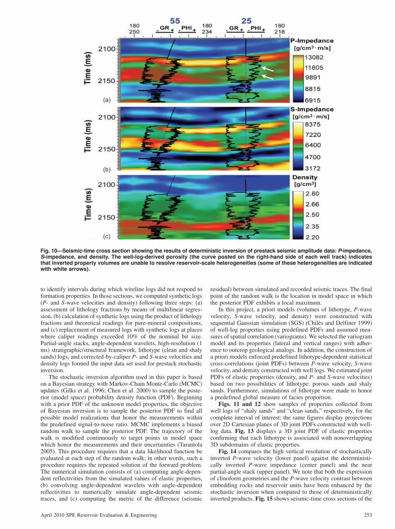
The synthetic models used for simulation included reservoir units with thickness above and below the vertical resolution of the simulated seismic amplitude data (Fig. 22). We first analyzed the inversion parameter that exerted the strongest influence on inversion products obtained from field data, namely the assumed lithotype proportion. The upper panels of Fig. 23 display initial models constructed with assumed lithotype proportions between clean sand and shaly sands of 0.2/0.8 (Fig. 23a) and 0.4/0.6 (Fig. 23b); remaining inversion parameters were kept the same as in previous sections of this paper. The impact of the difference of initial models on inversion results is evident in the cross sections of Fig. 23a. Lower panels display inversion results derived from the synthetic models. We note that lithotype distributions are almost identical, thereby indicating a negligible dependence of inversion products on the assumed global lithotype proportion.

Fig. 24 describes the sensitivity of inversion results (P-wave velocity) to the choice of lateral variogram range. Blue colors identify low-velocity values typical of reservoir units in the actual field data. The upper panels of Fig. 24 describe a priori models constructed with lateral variogram ranges of 900 (Fig. 24a) and 1500 m (Fig. 24b). We confirm that variogram lateral range exerts a significant control over the inverted spatial distribution of reservoir units. For purposes of cross validation of inversion results, Well S3 (see Fig. 24) was not included in the construction of a priori property models. We note that the upper reservoir unit in Well S3, indicated with the white arrows, is poorly defined by the synthetic seismic amplitude data. The lower panels of Fig. 24 show spatial distributions of P-wave velocity inverted with different values of lateral variogram range. In both cases, the thin layer in the upper section of Well S3 is delineated accurately regardless of the var-iogram lateral range used to construct the a priori model. Fig. 25 displays the results of a blind-well test in the location of Well S3. We note that the same thin reservoir unit, which was not resolved with deterministic inversion (Fig. 22), is now resolved accurately with stochastic inversion.

Finally, we performed a sensitivity analysis of inversion prod-ucts to the selection of stratigraphic framework. Fig 26 describes the results from this exercise. The upper panels in that figure

(a) (b)

Density, g/cm3

Fig. 21—Synthetic model of elastic properties (P-wave velocity, S-wave velocity, and density) interpolated from well logs and used to generate the synthetic prestack seismic amplitude data (a). The three synthetic partial-angle stacks (PAS) numerically simulated with the convolution of angle-dependent wavelets and the corresponding angle-dependent reflectivity volumes (b).


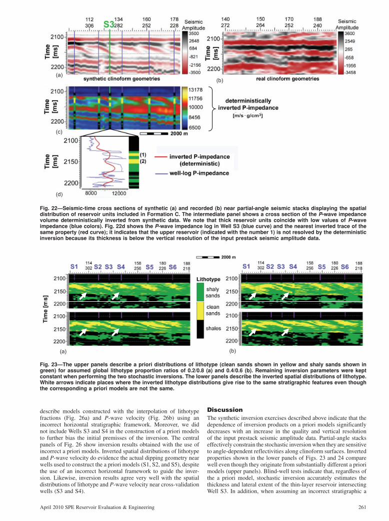
describe models constructed with the interpolation of lithotype fractions (Fig. 26a) and P-wave velocity (Fig. 26b) using an incorrect horizontal stratigraphic framework. Moreover, we did not include Wells S3 and S4 in the construction of a priori models to further bias the initial premisses of the inversion. The central panels of Fig. 26 show inversion results obtained with the use of incorrect a priori models. Inverted spatial distributions of lithotype and P-wave velocity do evidence the actual dipping geometry near wells used to construct the a priori models (S1, S2, and S5), despite the use of an incorrect horizontal framework to guide the inver-sion. Likewise, inversion results agree very well with the spatial distributions of lithotype and P-wave velocity near cross-validation wells (S3 and S4).

Discussion The synthetic inversion exercises described above indicate that the dependence of inversion products on a priori models significantly decreases with an increase in the quality and vertical resolution of the input prestack seismic amplitude data. Partial-angle stacks effectively constrain the stochastic inversion when they are sensitive to angle-dependent reflectivities along clinoform surfaces. Inverted properties shown in the lower panels of Figs. 23 and 24 compare well even though they originate from substantially different a priori models (upper panels). Blind-well tests indicate that, regardless of the a priori model, stochastic inversion accurately estimates the thickness and lateral extent of the thin-layer reservoir intersecting Well S3. In addition, when assuming an incorrect stratigraphic a

(d)

(b)(a)

(c)

[m/s⋅g/cm3]

Fig. 22—Seismic-time cross sections of synthetic (a) and recorded (b) near partial-angle seismic stacks displaying the spatial distribution of reservoir units included in Formation C. The intermediate panel shows a cross section of the P-wave impedance volume deterministically inverted from synthetic data. We note that thick reservoir units coincide with low values of P-wave impedance (blue colors). Fig. 22d shows the P-wave impedance log in Well S3 (blue curve) and the nearest inverted trace of the same property (red curve); it indicates that the upper reservoir (indicated with the number 1) is not resolved by the deterministic inversion because its thickness is below the vertical resolution of the input prestack seismic amplitude data.

(b)(a)

Fig. 23—The upper panels describe a priori distributions of lithotype (clean sands shown in yellow and shaly sands shown in green) for assumed global lithotype proportion ratios of 0.2/0.8 (a) and 0.4/0.6 (b). Remaining inversion parameters were kept constant when performing the two stochastic inversions. The lower panels describe the inverted spatial distributions of lithotype. White arrows indicate places where the inverted lithotype distributions give rise to the same stratigraphic features even though the corresponding a priori models are not the same.


priori model, stochastic inversion properly detected the thin-layer reservoir but the geometrical reconstruction was poor.

When seismic amplitude data do not evidence the actual res-ervoir geometry, either because of their low vertical resolution or because of the high degree of facies amalgamation, the reliability of inversion products becomes increasingly dependent on param-eters used to construct a priori models and on the choice of inver-sion parameters. In such cases, the stochastic inversion loses its ability to narrow down the likely range of solutions in model space that simultaneously honor both the seismic amplitude data and the well logs, thereby increasing the degree of non-uniqueness.

On the basis of the above observations with synthetic models, and fully aware of the limitations of signal-to-noise ratio, angular range, and vertical resolution of the recorded seismic amplitude data in the study area, we directed a considerable portion of our efforts to the construction of a priori models that reproduced the assumed reservoir architecture. In addition, we conducted a large number of cross-validation and blind-well tests to appraise the non-uniqueness and vertical resolution of inversion results.

On the basis of our experience, we strongly recommend that the stochastic inversion be preceded by a systematic analysis of the influence of a priori models and inversion parameters on inversion

(b)(a)

Fig. 24—Sensitivity of inversion products to the assumed variogram lateral range. The upper panels describe a priori models of P-wave velocity constructed with a 900- (a) and 1500-m (b) lateral variogram range, and without the use of Well S3 (which was kept aside as a blind well). The lower panels describe inverted products. In both cases, the thin layer included in the upper section of Well S3 (indicated with a white arrow) is delineated accurately by the inversion regardless of the parameters used to construct the a priori model.

Density [g/cm3]

Fig. 25—Blind-well test of stochastic inversion products performed at the location of Well S3. The reservoir unit identified with the number 1 is not resolved with deterministic inversion (see Fig. 22). The same reservoir unit was resolved consistently with stochastic inversion regardless of the a priori model or the specific choice of inversion parameters (e.g., variogram type, vari-ogram range, lithotype proportion).


products. Numerical simulation of synthetic reservoir models constructed with available wells and knowledge of stratigraphic architecture provides sufficient guidance to quantify non-unique-ness, reliability, and vertical resolution of inversion products.

ConclusionsJoint stochastic inversion of well logs and prestack seismic ampli-tude data enabled the accurate detection and spatial delineation of reservoir units otherwise poorly resolved with deterministic seismic inversion. The stochastic inversion of field data pursued in this paper yielded P- and S-wave velocity volumes with a vertical resolution of 10–15 m, compared to the vertical resolution of 25–30 m associated with deterministic inversion. This enhancement in vertical resolution allowed us to delineate most reservoir-scale heterogeneities. Moreover, cosimulation of porosity from inverted elastic properties enabled the spatial delineation of clean sands with the best storage conditions.

In cases in which the available seismic amplitude data were not sensitive to reservoir geometry, we found that inversion products were biased by both the a priori models and the inversion param-eters themselves. The only possible way to appraise non-unique-ness and reliability of inversion products derived from similar data sets is to perform a systematic study of the sensitivity of inversion products to a priori models and inversion parameters. Non-unique-ness of inversion products can be appraised with: (a) blind-well tests at each well location and (b) checks of the cross correlation between recorded and simulated prestack seismic amplitudes. Exercises with synthetic analog models indicated that stochastic inversion successfully reproduced clinoform configurations with noise-free seismic amplitude data.

The use of a priori models in close agreement with the under-lying stratigraphic framework effectively decreases the degree of non-uniqueness of inversion products. We obtained practically the same spatial distributions of lithotype and elastic properties with different a priori models and inversion parameters. All stochastic inversion tests performed over synthetic models using the correct stratigraphic framework successfully detected and delineated thin-bed reservoirs.

The gain in vertical resolution of stochastic inversion, compared to that of deterministic inversion, is a direct consequence of good-

(b)(a)

(c)

Fig. 26—Sensitivity of inversion products to the stratigraphic framework used to construct a priori models. The upper panels describe the spatial distributions of lithotype (a) and P-wave velocity (b) interpolated with an incorrect horizontal stratigraphic model (stratigraphic layering parallel to top and base). Note that the stratigraphic framework used to simulate the synthetic seismic amplitude data is similar to the one shown in Fig. 26c. The middle panels describe the inversion products. The inverted lithotype (a) and P-wave velocity (b) volumes indicate that the dipping-layer geometry is reconstructed properly by the inversion, despite the use of an incorrect a priori model.

quality logs, presence of several wells, and proximity of wells. Blind-well tests confirmed that absence of wells at key locations in the stratigraphic model decreased the resolution of inversion prod-ucts to that of properties obtained with deterministic inversion.

AcknowledgmentsThe authors would like to thank PDVSA for providing the data set used for this research study. We remain grateful to Fugro-Jason for their software support and to Elizabeth Fisher for her technical advice during the inversion phase of the study. Our gratitude goes to Jeff Kane (Bureau of Economic Geology of The University of Texas at Austin) for his assistance during the well-log petrophysi-cal evaluation. The work reported in this paper was funded by The University of Texas at Austin’s Research Consortium on Forma-tion Evaluation, jointly sponsored by Anadarko, Aramco, Baker-Hughes, BHP-Billiton, BP, BG, ConocoPhillips, Chevron, ENI, ExxonMobil, Halliburton, Hess, Marathon, Mexican Institute for Petroleum, Nexen, Petrobras, RWE, Schlumberger, StatoilHydro, TOTAL, and Weatherford.

ReferencesAki, K. and Richards, P.G. 1980. Quantitative Seismology, Theory and

Methods, 535. New York City: W.H. Freeman & Co.Aquino, R., Figueroa, L., Prieto, M., Salazar, R., Garcia, E., Kupecz, J., and

Hernandez, E. 1997. Sedimentological study of cores and correlation with well-logs, “O” Limestone, Barinas Basin, Venezuela. Abstract P A5 presented at the Annual AAPG-SEPM-EDM-DPA-DEG Conven-tion, Dallas, 6–9 April.

Bejarano, C. 2000. Sequence analysis and sedimentology of the Gobernador Formation, Barina Basin, Venezuela. Proc., VII Simposio Bolivariano de Exploración Petrolera en las Cuencas Subandinas, Venezuela, 1–26.

Castagna, J.P. and Backus, M.M. 1993. Offset-Dependent Reflectivity—Theory and Practice of AVO Analysis, No. 8, 348. Tulsa: Investigations in Geophysics, Society of Exploration Geophysicists.

Chen, M.-H., Shao, Q.-M., and Ibrahim, J.G. 2000. Monte Carlo Methods in Bayesian Computation, 375. New York City: Springer Series in Statistics, Springer-Verlag.

Chilès, J.-P. and Delfiner, P. 1999. Geostatistics: Modeling Spatial Uncer-tainty, 695. New York City: Wylie Series in Probability and Statistics, John Wiley & Sons.


Contreras, A. and Torres-Verdín, C. 2005. Sensitivity analysis of fac-tors controlling AVA simultaneous inversion of 3D partially stacked seismic data: application to deepwater hydrocarbon reservoirs in the central Gulf of Mexico. SEG Expanded Abstracts 24 (CH3): 464. doi: 10.1190/1.2144355.

Contreras, A., Torres-Verdín, C., Chesters, W., Kvien, K., and Fasnacht, T. 2005. Joint stochastic inversion of 3D pre-stack seismic data and well logs for high-resolution reservoir characterization and petrophysi-cal modeling: application to deepwater hydrocarbon reservoirs in the central Gulf of Mexico. SEG Expanded Abstracts 24 (RC2): 1343. doi: 10.1190/1.2147935.

Contreras, A., Torres-Verdín, C., Chesters, W., Kvien, K., and Fasnacht, T. 2006. Extrapolation of Flow Units Away From Wells With 3D Pre-Stack Seismic Amplitude Data: Field Example. Petrophysics 47 (3): 223–238.

Debeye, H.W.J. and van Riel, P. 1990. Lp-Norm Deconvolution. Geo-physical Prospecting 38 (4): 381–404. doi: 10.1111/j.1365-2478.1990.tb01852.x.

Dewan, J. 1983. Essentials of Modern Open-Hole Log Interpretation, 351. Tulsa: PennWell Publishing Company.

Fowler, J., Bogaards, M., and Jenkins, G. 2000. Simultaneous Inversion of the Ladybug prospect and derivation of a lithotype volume. SEG Expanded Abstracts 19 (RC4): 1517. doi: 10.1190/1.1815696.

Galloway, W. and Hobday, D. 1990. Terrigenous Clastic Depositional Systems: Applications to Fossil Fuel and Groundwater Resources, 485. Berlin: Springer-Verlag.

Gilks, W.R., Richardson, S., and Spiegelhalter, D.J. 1996. Markov Chain Monte Carlo in Practice: Interdisciplinary Statistics, 486. Boca Raton, Florida, USA: Chapman & Hall/CRC Press.

Goodway, W., Chen, T., and Downton, J. 1997. Improved AVO fluid detec-tion and lithology discrimination using Lamè petrophysical parameters; “� � “,”��”,&”�/� fluid stack”, from P and S inversions. SEG Expanded Abstracts 16 (AVO2): 183. doi: 10.1190/1.1885795.

Haas, A. and Dubrule, O. 1994. Geostatistical inversion—a sequential method for stochastic reservoir modeling constrained by seismic data. First Break 12 (11): 561–569.

Hilterman, F.J. 1983. Stratigraphic interpretation of seismic data. Continu-ing Education Lecture Series, AAPG School, Houston.

Merletti, G., Hlebszevitsch, J.C., and Torres-Verdín, C. 2003. Geostatis-tical inversion for the lateral delineation of thin-layer hydrocarbon reservoirs: a case study in San Jorge Basin, Argentina. SEG Expanded Abstracts 22 (IT2): 662. doi: 10.1190/1.1818017.

Pendrel, J. 2001. Seismic Inversion—The Best Tool for Reservoir Charac-terization. CSEG Recorder 26 (1): Feature Article.

Pendrel, J. and van Riel, P. 1997. Methodology for seismic inversion and mod-eling: a Western Canadian reef example. CSEG Recorder 12 (5): 5–15.

Rutherford, S. and Williams, R. 1989. Amplitude-versus-offset variations in gas sands. Geophysics 54 (6): 680–688.

Sheriff, R.E. and Geldart, L.P. 1982. Exploration Seismology, 575. Cam-bridge, UK: Cambridge University Press.

Tarantola, A. 2005. Inverse Problem Theory and Methods for Model Param-eter Estimation, 333. Philadelphia, Pennsylvania, USA: SIAM.

Tatham, R.H., McCormack, M.D., Neitzel, E.B., and Winterstein, D.F. 1991. Multicomponent Seismology in Petroleum Exploration, No. 6, 248. Tulsa, Oklahoma: Investigations in Geophysics, Society of Explo-ration Geophysicists (SEG).

Torres-Verdín, C., Victoria, M., Merletti, G., and Pendrel, J. 1999. Trace-based and geostatistical inversion of 3-D seismic data for thin-sand delineation: an application in San Jorge Basin, Argentina. The Leading Edge 18 (9): 1070–1077.

Walker, R.G. and Plint, A.G. 1992. Wave- and storm-dominated shallow marine systems. In Facies Models: Response to Sea-Level Change, ed. R.G. Walker and N.P. James, 219–238. St. John’s, Newfoundland, Canada: Geological Association of Canada.

Germán Merletti holds a degree in geology from the National U. of Cordoba, Argentina (1995). E-mail: [email protected]. He worked for YPF S.A. as a petrophysicist and res-ervoir geologist. In March 2000, Merletti began working with integrated projects that included well-log correlation, petro-physics and seismic inversion for Repsol-YPF. In August 2004, he jointed the Masters program at the Jackson School of Geosciences of The U. of Texas at Austin where he worked for the Research Consortium on Formation Evaluation as Graduate Research Assistant on Seismic Inversion. Merletti now works at BP as a petrophysicist and reservoir modeler. Carlos Torres-Verdín holds a PhD degree in engineering geo-science from the U of California at Berkeley (1991). E-mail: [email protected]. During 1991–1997, he held the posi-tion of research scientist with Schlumberger-Doll Research. From 1997–1999, Torres-Verdín was reservoir specialist and technology champion with YPF (Buenos Aires). Since 1999, he has been affiliated with the Department of Petroleum and Geosystems Engineering of the U. of Texas at Austin, where he currently holds the position of Zarrow Centennial Professor in Petroleum Engineering and conducts research on bore-hole geophysics, formation evaluation, well logging, and inte-grated reservoir characterization. Torres-Verdín is the founder and director of the Research Consortium on Formation Evaluation at the U. of Texas at Austin. He is recipient of the 2006 Distinguished Technical Achievement Award from the SPWLA and the 2008 SPE Formation Evaluation.

Documents

Detection and Spatial Delineation of Thin-Sand Sedimentary ... · evidenced in seismic-amplitude sections. Fig. 3 is a seismic cross section displaying high-angle clino-forms. Dip