University of Nebraska - LincolnDigitalCommons@University of Nebraska - Lincoln

Papers in Natural Resources Natural Resources, School of

6-2011

Detecting Spatiotemporal Changes of CornDevelopmental Stages in the U.S. Corn Belt UsingMODIS WDRVI DataToshihiro Sakamoto

Brian D. WardlowUniversity of Nebraska-Lincoln, bwardlow2@unl.edu

Anatoly A. GitelsonUniversity of Nebraska-Lincoln, agitelson2@unl.edu

Follow this and additional works at: https://digitalcommons.unl.edu/natrespapers

Part of the Natural Resources and Conservation Commons

This Article is brought to you for free and open access by the Natural Resources, School of at DigitalCommons@University of Nebraska - Lincoln. Ithas been accepted for inclusion in Papers in Natural Resources by an authorized administrator of DigitalCommons@University of Nebraska - Lincoln.

Sakamoto, Toshihiro; Wardlow, Brian D.; and Gitelson, Anatoly A., "Detecting Spatiotemporal Changes of Corn DevelopmentalStages in the U.S. Corn Belt Using MODIS WDRVI Data" (2011). Papers in Natural Resources. 352.https://digitalcommons.unl.edu/natrespapers/352

1926 IEEE TRANSACTIONS ON GEOSCIENCE AND REMOTE SENSING, VOL. 49, NO. 6, JUNE 2011

Detecting Spatiotemporal Changes of CornDevelopmental Stages in the U.S. Corn Belt

Using MODIS WDRVI DataToshihiro Sakamoto, Brian D. Wardlow, and Anatoly A. Gitelson

Abstract—The dates of crop developmental stages are impor-tant variables for many applications including assessment of theimpact of abnormal weather on crop yield. Time-series 250-mvegetation-index (VI) data acquired from the Moderate ResolutionImaging Spectroradiometer (MODIS) provide valuable informa-tion for monitoring the spatiotemporal changes of corn growthacross large geographic areas. The goal of this study is to evalu-ate the performance of a new crop phenology detection method,namely, two-step filtering (TSF), for revealing the spatiotemporalpattern of specific corn developmental stages (early vegetative:V2.5; silking: R1; dent: R5; mature: R6) over an eight-year period(2001–2008) across Iowa, Illinois, and Indiana using MODIS-derived Wide Dynamic Range VI data. Weekly crop progressreports produced by the U.S. Department of Agriculture NationalAgricultural Statistics Service (NASS) were used to assess theaccuracy of TSF-based estimates of corn developmental stages.The results showed that the corn developmental stages could beestimated with high accuracy (the root mean squared error rangedfrom 4.1 to 5.5 days, the determination coefficient ranged from0.66 to 0.84, and the coefficient of variation ranged from 2.1%to 3.7%) based on NASS-derived statistics on an agriculturalstatistics district level. In particular, the annual changes in thespatiotemporal patterns of the estimated silking stage had a highlevel of agreement with those of the NASS-derived statistics. Theseresults suggested that the TSF method could provide local-scaleinformation of corn phenological stages, which had an advantageover the NASS-derived statistics particularly in terms of the spa-tial resolution.

Index Terms—Agriculture, optical imaging, remote sensing,time series, vegetation mapping.

I. INTRODUCTION

THE U.S. Corn Belt, which comprises several midwesternstates, is one of the world’s largest corn production regions

and represents a major source of grain that is exported fromthe U.S. The majority of corn in this region is grown underrain-fed conditions. Considering that a crop’s physiologicalresponse (e.g., light-use efficiency, sterility, or transpirationrate) to extreme weather conditions varies depending on crop

Manuscript received May 4, 2010; revised August 6, 2010; acceptedNovember 16, 2010. Date of publication January 5, 2011; date of currentversion May 20, 2011. This work was supported by the Japanese Society forthe Promotion of Science (JSPS) under the JSPS Postdoctoral Fellowships forResearch Abroad.

T. Sakamoto is with the School of Natural Resources, University ofNebraska—Lincoln, Lincoln, NE 68588 USA, and also with the EcosystemInformatics Division, National Institute for Agro-Environmental Sciences,Tsukuba 305-8604, Japan (e-mail: sakamt@affrc.go.jp).

B. D. Wardlow and A. A. Gitelson are with the School of Natural Resources,University of Nebraska—Lincoln, Lincoln, NE 68588 USA.

Digital Object Identifier 10.1109/TGRS.2010.2095462

developmental stages, annual corn production can be associatedwith the spatiotemporal relationship between abnormal weatherconditions (e.g., flood, drought, or hail) and specific cropdevelopmental stages (e.g., early vegetative stage, floweringstage, or mature stage) on a regional scale. Moreover, deficientor excessive soil-moisture conditions and soil temperature inthe spring result in variable corn planting dates across largegeographic areas, as well as influence other crop managementdecisions. Although weather conditions are well monitored byweather station networks on a real-time basis, the practicalmethod that enables the spatiotemporal pattern of crop devel-opmental stages to be revealed has not been well established inthe U.S. Reliable archival records related to crop developmentalstages have been regularly recorded by the U.S. Departmentof Agriculture (USDA) National Agricultural Statistics Servicein crop progress reports (CPRs) (NASS-CPRs; reports arepublicly available at http://www.nass.usda.gov/). However,NASS-CPR records the progress of crop developmental stagesby the percent complete (area ratio) over a large administrativeunit. The geographic reporting unit, which is the entire state oragricultural statistics district (ASD; a substate region comprisedof multiple counties), is too large to reveal detailed spatialpatterns of crop developmental stages. It has been difficult toassess the effect of local weather-condition changes on cropproductivity with particular reference to the spatiotemporalpattern of crop phenology. Thus, remote-sensing techniques areexpected to present a reasonable solution to characterize local-scale annual changes in crop developmental stages over largeregions such as the U.S. Corn Belt.

Time-series vegetation-index (VI) data, which are obtainedby the Advanced Very High Resolution Radiometer or Mod-erate Resolution Imaging Spectroradiometer (MODIS), arecommonly used for acquiring phenological information aboutnatural vegetation or agricultural crops across large geographicareas [1]–[12]. The majority of existing phenology detectionmethods detect specific phenological stages in reference tolocal features in the time-series VI data based on prescribedthresholds [2], [3], [7], [13]–[16], logistic curve fitting [4],[8], [17]–[19], forward and backward lag periods of smoothedVI data (delayed moving average) [1], [20], [21], or met-rics such as maximum, minimum, and inflection points [5],[22]–[24]. Several studies estimate key phenological stagesusing a combination of time-series VI data and environmentalinformation such as humidity and temperature [6], [25], [26].The smoothed MODIS VI profile has been effectively used to

0196-2892/$26.00 © 2011 IEEE

SAKAMOTO et al.: DETECTING SPATIOTEMPORAL CHANGES OF CORN DEVELOPMENTAL STAGES 1927

produce agricultural land-use maps [27]–[31] and monitor char-acteristics of crop phenology [16], [22], [32]–[34] and croppingschedules at a regional scale with moderate resolution imagery(e.g., 250–500 m) [35]. Although these various approachesusing time-series VI data have demonstrated the capability tocharacterize spatiotemporal patterns of vegetation phenology,few of these studies quantitatively evaluated the accuracy ofthe results to capture the spatial variability and interannualchanges that occur in crop phenology across large geographicareas. In addition, most of these studies have estimated phe-nological stages defined by specific VI metrics (e.g., onset ofgreenness and senescence), which do not always correspond tospecific crop developmental stages defined in crop science (e.g.,emergence and mature stage). The phenology detection methodbased on specific VI metrics (e.g., greenness onset) is poten-tially affected by extensive weed cover growing before cropplanting [4]. Atmospheric conditions and moderate resolutionimagery with many mixed pixels (composite spectral–temporalsignal from multiple land-cover types) can also produce subtlenon-vegetation-related local features in the temporal VI profilethat can lead to errors in detecting the key phenological stageswith specific metrics (e.g., maximum point [36]) and reducethe estimation accuracy for tracking yearly changes of cropdevelopmental stages.

A new approach, the two-step filtering (TSF) method, hasbeen proposed to improve the performance of the MODIS-derived crop phenology dates [36]. The TSF method includesa simple smoothing procedure based on the wavelet-basedfilter to reduce noise components from temporal VI data (firststep) and a shape-model fitting procedure to estimate the datesof key phenological stages by overcoming the influence ofremaining subtle non-vegetation-related local features (secondstep). The TSF method can estimate the dates of the keyphenological stages of corn: early vegetative stage (V2.5),silking stage (R1), dent stage (R5), and mature stage (R6). Theestimation accuracy of corn developmental stages at the fieldscale was relatively high, i.e., early vegetative stage (V2.5):rmse = 3.7 days; silking stage: rmse = 2.9 days, dent stage:rmse = 7.0 days, and mature stage: rmse = 3.7 days. It wasalso verified that the TSF method is effective in revealing thecorn phenological stage variations at a regional scale. Region-average estimates calculated using the TSF method agreedwell with the USDA statistical data for three ASDs in easternNebraska (V2.5: rmse = 4.1 days; R1: rmse = 1.6 days; R5:rmse = 5.6 days; R6: rmse = 3.3 days). The preliminarydefined parameters of the TSF method were based on thespecific data collected in the experimental field sites locatedin eastern Nebraska, but we do not know how well the TSFmethod can be applied outside of the state. In addition, theASD-level statistical data used for regional-scale verificationin Nebraska were limited to only two years (2001 and 2002).Thus, it is necessary to test the accuracy of the TSF method inevaluation of interannual variations of corn phenological stagesacross a larger multistate region.

The objectives of this paper are as follows: 1) to apply theTSF method to characterize the spatiotemporal patterns of corndevelopmental stages across a three-state area of the U.S. CornBelt (Illinois, Indiana, and Iowa) using time-series MODIS

250-m VI data observed from 2001 to 2008 and 2) to assess theperformance of the TSF method for a spatial extrapolation ofcorn developmental stages on a multistate scale using statisticaldata derived from the weekly NASS-CPR.

II. STUDY AREA

The study area comprised three major corn-producingstates (Iowa, Illinois, and Indiana), where the target cornfields spread over 1000 km in an east–west direction (longi-tudes: from 84◦47′31′′ W to 96◦38′45′′ W) and over 730 kmin a north–south direction (latitudes: from 36◦58′21′′ N to43◦30′9′′ N). The total corn area harvested for grain was12.2 million ha in the three states in 2008. The total cornproduction was 131.9 million tons, which accounted for 42.9%of the total in the U.S. [37].

III. DATA AND METHODS

A. MODIS WDRVI

A time series of eight-day composite 250- and 500-mMODIS surface reflectance data (MOD09Q and MOD09A1,Collection 5, tiles: h10v04, h10v05, h11v04, and h11v05) from2001 to 2008 was used. The 500-m resolution blue-reflectance(Band 3) and day of year (DOY) data layers were resampled to250-m-resolution images using the nearest neighbor method.The blue-reflectance and DOY layers were used for residualcloud cover detection and time-series analysis in the wavelet-based filter, respectively. Even though the MODIS eight-daycomposite product is corrected for atmospheric effect [38] andprovides the best surface spectral-reflectance data for eacheight-day period selected by the constrained view-angle max-imum value composite method [39], the observed multitem-poral VI data still contain short-term fluctuations caused bypersistent cloud coverage, bidirectional reflectance distributionfunction effects, and mixed-pixel effects. Any pixel with a bluereflectance greater than 0.2 [31], [33], [40] was defined as thecloud-covered pixel and was treated as a missing observationin a preprocessing scheme of the wavelet-based filter. Then,the multitemporal VI data were smoothed to reduce the noisecomponents through wavelet transformation [33].

Although the TSF method is expected to be applicable toany time-series VI data such as Normalized Difference VI(NDVI [41]) and Enhanced VI [39], Wide Dynamic Range VI(WDRVI) was selected here because of its near-linear relation-ship with green leaf area index in a wide range of biomass,including the moderate-to-high-biomass growth stages [42]–[45]. WDRVI was calculated as [42]

WDRV I = (α× ρNIR − ρred)/(α× ρNIR + ρred) (1)

where ρNIR and ρred are the 250-m MODIS surface reflectancein the near-infrared (NIR: 841–875 nm, Band 2) and red (red:621–670 nm, Band 1) bands and α is a weighting coefficient(α = 0.2 was used in this study [43]).

WDRVI can also be obtained from NDVI by [46]

WDRV I = [(α+ 1)NDV I + (α− 1)]

/ [(α− 1)NDV I + (α+ 1)] . (2)

1928 IEEE TRANSACTIONS ON GEOSCIENCE AND REMOTE SENSING, VOL. 49, NO. 6, JUNE 2011

B. USDA/NASS-CDL

Target corn pixels were selected using NASS Cropland DataLayer (NASS-CDL), which classifies the spatial distribution ofspecific crop types on annual basis for selected states. The orig-inal NASS-CDL data were resampled from an original spatialresolution of 30 m (Landsat-based products)/56 m (AdvancedWide Field Sensor-based products) to 250 m to match theMODIS data. The percentage area of corn present was then cal-culated in each 250-m pixel across the three states of the studyarea where the TSF method was applied only on pixels contain-ing 75% or more corn. The area threshold (more than or equalto 75%) was arbitrarily determined by testing several thresholdsand evaluating the spatial distribution of the corn pixels thatmet that threshold across the study area. The 75% threshold wasselected because it provided a large sample of corn pixels acrossthe three states while ensuring that corn was the dominant covertype within each of these 250-m pixels [36]. The total area ofthe pixels selected as target cornfields was about 7.5 million ha,which accounted for 62% of the total harvested area in 2008.

C. TSF Method

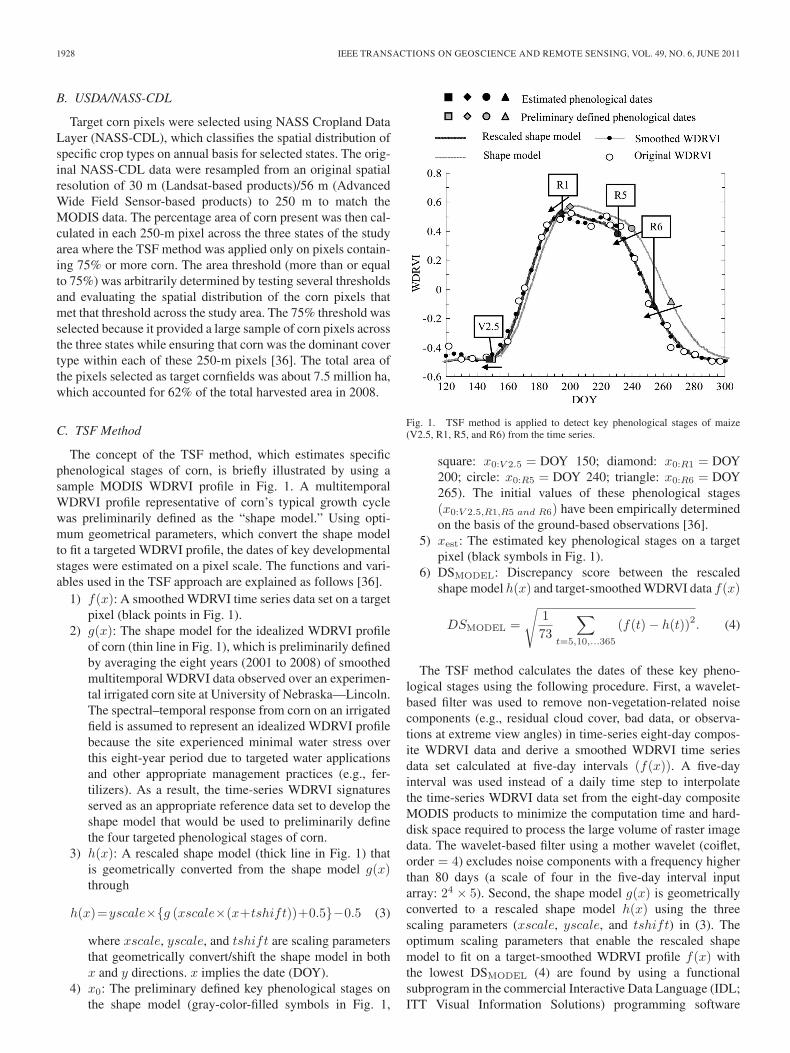
The concept of the TSF method, which estimates specificphenological stages of corn, is briefly illustrated by using asample MODIS WDRVI profile in Fig. 1. A multitemporalWDRVI profile representative of corn’s typical growth cyclewas preliminarily defined as the “shape model.” Using opti-mum geometrical parameters, which convert the shape modelto fit a targeted WDRVI profile, the dates of key developmentalstages were estimated on a pixel scale. The functions and vari-ables used in the TSF approach are explained as follows [36].

1) f(x): A smoothed WDRVI time series data set on a targetpixel (black points in Fig. 1).

2) g(x): The shape model for the idealized WDRVI profileof corn (thin line in Fig. 1), which is preliminarily definedby averaging the eight years (2001 to 2008) of smoothedmultitemporal WDRVI data observed over an experimen-tal irrigated corn site at University of Nebraska—Lincoln.The spectral–temporal response from corn on an irrigatedfield is assumed to represent an idealized WDRVI profilebecause the site experienced minimal water stress overthis eight-year period due to targeted water applicationsand other appropriate management practices (e.g., fer-tilizers). As a result, the time-series WDRVI signaturesserved as an appropriate reference data set to develop theshape model that would be used to preliminarily definethe four targeted phenological stages of corn.

3) h(x): A rescaled shape model (thick line in Fig. 1) thatis geometrically converted from the shape model g(x)through

h(x)=yscale×{g (xscale×(x+tshift))+0.5}−0.5 (3)

where xscale, yscale, and tshift are scaling parametersthat geometrically convert/shift the shape model in bothx and y directions. x implies the date (DOY).

4) x0: The preliminary defined key phenological stages onthe shape model (gray-color-filled symbols in Fig. 1,

Fig. 1. TSF method is applied to detect key phenological stages of maize(V2.5, R1, R5, and R6) from the time series.

square: x0:V 2.5 = DOY 150; diamond: x0:R1 = DOY200; circle: x0:R5 = DOY 240; triangle: x0:R6 = DOY265). The initial values of these phenological stages(x0:V 2.5,R1,R5 and R6) have been empirically determinedon the basis of the ground-based observations [36].

5) xest: The estimated key phenological stages on a targetpixel (black symbols in Fig. 1).

6) DSMODEL: Discrepancy score between the rescaledshape model h(x) and target-smoothed WDRVI data f(x)

DSMODEL =

√1

73

∑t=5,10,...365

(f(t)− h(t))2. (4)

The TSF method calculates the dates of these key pheno-logical stages using the following procedure. First, a wavelet-based filter was used to remove non-vegetation-related noisecomponents (e.g., residual cloud cover, bad data, or observa-tions at extreme view angles) in time-series eight-day compos-ite WDRVI data and derive a smoothed WDRVI time seriesdata set calculated at five-day intervals (f(x)). A five-dayinterval was used instead of a daily time step to interpolatethe time-series WDRVI data set from the eight-day compositeMODIS products to minimize the computation time and hard-disk space required to process the large volume of raster imagedata. The wavelet-based filter using a mother wavelet (coiflet,order = 4) excludes noise components with a frequency higherthan 80 days (a scale of four in the five-day interval inputarray: 24 × 5). Second, the shape model g(x) is geometricallyconverted to a rescaled shape model h(x) using the threescaling parameters (xscale, yscale, and tshift) in (3). Theoptimum scaling parameters that enable the rescaled shapemodel to fit on a target-smoothed WDRVI profile f(x) withthe lowest DSMODEL (4) are found by using a functionalsubprogram in the commercial Interactive Data Language (IDL;ITT Visual Information Solutions) programming software

SAKAMOTO et al.: DETECTING SPATIOTEMPORAL CHANGES OF CORN DEVELOPMENTAL STAGES 1929

named “CONSTRAINED_MIN,” which is designed foroptimization analysis and is based on the Generalized ReducedGradient Code [47]. Lastly, objective phenological stages (xest)are calculated using the optimum scaling parameters with thepreliminary defined dates of key phenological stages (x0) from

xest = xscale× (x0 + tshift). (5)

See [5] and [36] for further details about the wavelet-based filterand the TSF method.

D. NASS-CPR

USDA/NASS releases basic phenological information forcorn and other crops in weekly CPRs that can serve as a surro-gate for ground-based observations when evaluating the perfor-mance of remote-sensing-based crop phenology estimates at aregional (i.e., multistate) scale. These reports show the percentcomplete (area ratio) of crop fields that has either reached orcompleted a specific phenological stage over a given geogra-phic area. USDA/NASS designates the timing of a phenologicalstage when more than 50% of plants reach the objective devel-opmental stage on a field level. According to USDA/NASS’s“Crop progress and condition survey and estimating proce-dures,” the crop progress and condition surveys are based onquestionnaires returned weekly from more than 5000 reporters,who conduct visual observations of farms and frequently contactfarmers. The corn phenological stages are defined as follows:“Emerged: as soon as the plants are visible; Silking: the emer-gence of silklike strands from the end of ears; Dough: normallyhalf of the kernels are showing dent with some thick or dough-like substance in all kernels; Dent: occurs when all kernels arefully dented and the ear is firm and solid and there is no milkpresent in most kernels; and Mature: plant is considered safefrom frost and corn is about ready to be harvested withshucks opening and no green foliage present” (Definitions fromUSDA/NASS website available at http://www.nass.usda.gov/Charts_and_Maps/Crop_Progress_&_Condition/). The geo-graphic reporting unit for the NASS-CPR varies by state.Some states, including Indiana, report the crop progress dataat the state level while other states report the ASD-level data.For this research, ASD-level crop progress data were availablefor several study years in Illinois (2001 to 2008) and Iowa(2006 to 2008).

The weekly values of the percent complete reported in theNASS-CPR were temporally interpolated to a daily basis inorder to estimate the date when each phenological stage reachedspecific thresholds (5%, 25%, 50%, 75%, and 95%) at the ASDor state level. The accuracy of the TSF method for estimatingthe corn phenological stage was quantitatively evaluated at theASD level for Illinois and Iowa. The coefficient of variation(CV), the root mean squared error (rmse), and determinationcoefficient (R2) were used as criterion for accuracy assessment.

The rmse and CV were calculated by the following:

rmse =

√1

N

∑i=1,2,...N

(yi − xi + bias)2 (6)

CV =rmse

x× 100 (7)

where xi is the date of NASS-CPR-derived statistics whenpercent complete of target phenological stage reached 50%at an ASD level, yi is the date of MODIS-derived estimates,N is the number of estimations (y) compared with statis-tical data (x), and bias is the bias-correction value. Whenassessing the emerged stage, we assigned the bias-correctionvalue (−10 days) to bias for filling the time lag causedby the different definitions between the NASS-CPR-derivedemerged stage and the MODIS-estimated early vegetation stage(V2.5). For the other phenological stages of silking stage (R1),dent stage (R5), and mature stage (R6), we assigned zeroto bias.

The Nash–Sutcliffe (NS) model efficiency coefficient [48],which is often used for assessing the predictive power ofhydrological models, is a suitable index for quantifying thedegree of coincidence between two time-series profiles. Thedynamic range of NS is from minus infinity to one. If the NSis closer to one here, the temporal profile the MODIS-derivedestimations is in excellent agreement with that of the NASS-CPR-derived statistics. The NS was defined as follows:

NS = 1−∑

(p(t)− q(t+ bias))2∑(p(t)− q)2

(8)

where t is the date when the statistical values of NASS-CPRwere collected, p(t) is the percent complete of a phenologicalstage reported in the NASS-CPR at the date t, q(t) is the percentcomplete of a phenological stage derived from the MODISestimates on an ASD level at the date given by t+ bias, andbias is the bias-correction value. As for the silking stage onlyof Iowa, we assessed the estimation accuracy in two differentways: 1) with the bias correction (bias = +5 days) and 2)without the bias correction (bias = 0). On the other cases, weassigned zero to bias.

The NASS-CPR-derived statistics on a state level were usedonly in visual evaluation of the spatiotemporal distribution ofthe MODIS-estimated silking (R1) dates for missing values ofASD-level statistics in Iowa and Indiana.

IV. RESULTS AND DISCUSSION

A. Validation of the TSF Method for Estimating KeyPhenological Stages of Corn on an ASD Level

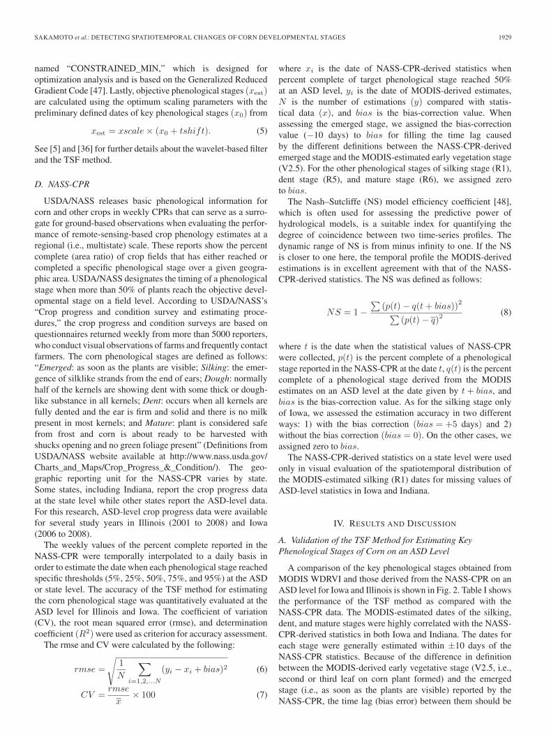
A comparison of the key phenological stages obtained fromMODIS WDRVI and those derived from the NASS-CPR on anASD level for Iowa and Illinois is shown in Fig. 2. Table I showsthe performance of the TSF method as compared with theNASS-CPR data. The MODIS-estimated dates of the silking,dent, and mature stages were highly correlated with the NASS-CPR-derived statistics in both Iowa and Indiana. The dates foreach stage were generally estimated within ±10 days of theNASS-CPR statistics. Because of the difference in definitionbetween the MODIS-derived early vegetative stage (V2.5, i.e.,second or third leaf on corn plant formed) and the emergedstage (i.e., as soon as the plants are visible) reported by theNASS-CPR, the time lag (bias error) between them should be

1930 IEEE TRANSACTIONS ON GEOSCIENCE AND REMOTE SENSING, VOL. 49, NO. 6, JUNE 2011

Fig. 2. Comparison of key phenological stages between the MODIS-derived estimation and the NASS-CPR.

TABLE IACCURACY ASSESSMENT OF THE MODIS-ESTIMATED PHENOLOGICAL STAGES AGAINST THE

ASD-LEVEL STATISTICAL DATA IN NASS CROP PROGRESS REPORTS

considered when assessing the estimation accuracy. Accordingto [49], a new leaf on a young corn plant forms approximatelyevery four days. If this rule is applicable to the corn growth inIowa and Illinois, the approximate ten-day difference observedbetween the MODIS-estimated dates of early vegetative stage(V2.5) and the NASS-CPR-derived dates of emerged stage(Fig. 2) is within the expected time lag between the twodifferent stages.

The performance of the TSF method for estimating the cornphenological stages in this study was similar to that observed inthe previous study [36]. The estimation accuracy for the silkingstage in this study (rmse = 4.1 days, R2 = 0.84, and n = 99)was higher than those of the other phenological stages at theASD level, as well as of the results from the previous easternNebraska study for 2001–2002 (rmse = 1.6 days, R2 = 0.78,and n = 6) [36]. The possible reason why the estimation accu-racy for the silking stage in the previous study was higher thanthat in this study was that most cornfields in Iowa and Illinoisare rain-fed fields; Nebraska has a higher percentage area ofirrigated cornfields (61% in 2008 [37]). The previous studysuggested that the rmse of silking stage estimation for irrigated

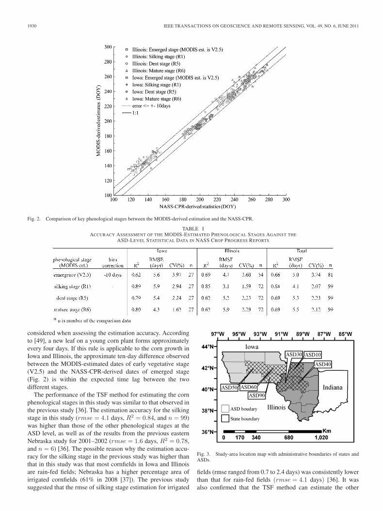
Fig. 3. Study-area location map with administrative boundaries of states andASDs.

fields (rmse ranged from 0.7 to 2.4 days) was consistently lowerthan that for rain-fed fields (rmse = 4.1 days) [36]. It wasalso confirmed that the TSF method can estimate the other

SAKAMOTO et al.: DETECTING SPATIOTEMPORAL CHANGES OF CORN DEVELOPMENTAL STAGES 1931

Fig. 4. Comparison of yearly changes in key phenological stages between (gray/white triangle) the MODIS-derived estimation and (black triangle) the NASS-CPR on the two districts (ASD50 of Iowa and ASD40 of Illinois). (A, E) MODIS-derived V2.5 stage or the NASS-derived emerged stage. (B, F) Silking (R1)stage. (C, G) Dent (R5) stage. (D, I) Mature (R6) stage.

phenological stages with reasonable accuracy (rmse rangedfrom 5.0 to 5.5 days and R2 ranged from 0.66 to 0.69), whichwas similar to the results from the pixel-scale evaluation con-ducted in the previous Nebraska study (rmse = 3.7− 7.0 daysand R2 = 0.39− 0.81) [36]. According to the results of CV(Table I), the estimation accuracy for early vegetative stage(V2.5) was not extremely high (CV ranged from 3.6% to 4.0%),but tended to be lower than those for the other stages (CVs ofsilking, dent, and mature stages ranged from 1.6% to 3.0%).The weak VI signal of the early vegetative stage due to lowvegetation fraction may result in slightly higher CVs than thoseof other phenological stages.

B. Comparison of Yearly Changes of the Key PhenologicalStages Between the MODIS Estimates and the NASS-CPRStatistics in Iowa and Illinois

Fig. 4 shows the yearly changes of the key phenologicalstages derived from the MODIS and the NASS-CPR for twodistricts called ASD50 in Iowa and ASD40 in Illinois (Fig. 3).The two districts were selected because they are located inthe center of each state and were appropriate to representcharacteristic yearly changes of the target phenological stagesin both states. The yearly changes in MODIS-derived estimates,particularly for the silking and mature stages, were consistentwith those dates in the NASS-CPR statistics over the eight-year

1932 IEEE TRANSACTIONS ON GEOSCIENCE AND REMOTE SENSING, VOL. 49, NO. 6, JUNE 2011

Fig. 5. Histogram of NS efficiency when comparing weekly percent complete of key phenological stages between the NASS-derived statistics and the MODIS-derived estimates on an ASD level in (a) Iowa and (b) Illinois. ∗The bias correction (−10 days) was conducted. ∗∗The bias correction (+5 days) was conductedonly for silking stage in Iowa.

period. The percentage of crop completing each phenologicalstage is expressed as the accumulated area ratio (i.e., completedarea divided by total planted area of corn) at the ASD level,which corresponds to error bars in Fig. 4. There are somedifferences in the observed range of percent complete (from 5%to 95%) between the MODIS-derived estimates and the NASS-CPR statistics, depending on the phenological stage. The resultsof the NS efficiency (Fig. 5) showed that the MODIS-derivedestimates corresponded well with the NASS-derived statistics interms of time-series variation, except the silking stage of Iowaand the dent stages of both states. The percentages of samplesachieving high NS values (NS => 0.7) in Illinois were 70.4%(n = 38) for emerged stage, 86.1% (n = 62) for silking stage,58.3% (n = 42) for dent stage, and 76.4% (n = 55) for maturestage while those in Iowa were 74.1% (n = 20) for emergedstage, 33.3% (n = 9) for silking stage (without the bias correc-tion), 48.1% (n = 13) for dent stage, and 70.4% (n = 19) formature stage. When the bias correction was not applied for thesilking stage in Iowa, the histogram distribution of NS for thesilking stage (Fig. 5(a), gray bar) was extremely skewed towardlower categories in comparison with those in Illinois (Fig. 5(b),gray bar). On the basis of the NS histogram, the estimationaccuracy for the silking stage in Iowa was considerably lowereven though R2 (0.89) and CV (2.94%) were not much lowerthan those of the other stages (Table I). This suggested thata bias error was included in the NASS-CPR data. Accordingto Fig. 2 (gray diamonds) and Fig. 4(b) (black diamonds),the NASS-derived silking stages were obviously later than theMODIS-derived estimates in Iowa, which were different fromthose in Illinois. When we assigned the bias-correction value(+5 days), which was empirically determined in reference toFig. 2, to (8) in order to investigate the effect of the biascorrection on the NS value, the NS-based estimation accuracyof the MODIS-derived silking stage in Iowa was drasticallyimproved by the bias correction (+5 days). The percentageof samples achieving the high NS value (NS => 0.7) for thesilking stage in Iowa was increased from 33.3% (n = 9, withoutthe bias correction) to 96.3% (n = 26, with the bias correctionof +5 days). This implied the possibility that the statisticalvalue of the silking stage reported by NASS-CPR for Iowaincluded some bias component. We could not figure out whatis behind this bias error observed only in Iowa. As will be

discussed in detail in the next section, this apparent bias isillustrated by the sharp contrast and lack of a gradual spatialgradation across the state border between Iowa and Illinois inthe ASD-level silking-stage maps derived from the NASS-CPRstatistics [Fig. 6(v)–(x)].

The results confirmed that the TSF method using the MODISWDRVI data was very effective for estimating the region-average dates of key phenological stages in terms of interannualvariations. However, as can be expected from the fact thatthe NS value was not always high for all samples, the TSFmethod has the potential to overlook fields where a specificphenological stage was much earlier or later than the regionaverage. Taking into consideration the fact that the progressionrate of reproductive stages depends on environmental factorsincluding temperature, soil water availability, available soilnutrients, and hybrid maturity differences [49], it should benoted that the temporal profile of WDRVI reflects growth andsenescence rates of green vegetation, but does not have directconnection with the degrees of kernel development covered byhusks below vegetative canopy.

C. Spatial Comparison of the Dates of Silking StageBetween the MODIS-Derived Estimates and theNASS-CPR-Derived Statistics

Heat and drought stress between the late vegetative growthstage (V10–V15) and the dent stage (R5) can cause a decreasein the final yield of corn [50]. In particular, the pollination andfertilization period around the silking stage (R1) is the mostsensitive crop developmental stage to drought stress, becausedrought conditions cause poor or incomplete pollination, whichresults in a high percentage of sterility. Thus, the MODIS-derived estimates, which can rearrange gridded meteorologicaldata (reanalysis data) in chronological order based on crop phe-nology, would enable us to assess how much the spatiotempo-ral correspondence between specific crop developmental stagevariations and abnormal weather conditions (e.g., drought)impacts final crop yields across large geographic areas. Fig. 6shows a comparison between the MODIS-derived county-levelestimates of the silking stage and the corresponding ASD-levelstatistics in the NASS-CPRs (defined as 50% of corn in theASD having completed the silking stage) from 2001 to 2008.

SAKAMOTO et al.: DETECTING SPATIOTEMPORAL CHANGES OF CORN DEVELOPMENTAL STAGES 1933

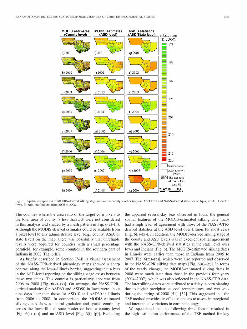
Fig. 6. Spatial comparison of MODIS-derived silking stage on (a–h) a county level or (i–p) an ASD level and NASS-derived statistics on (q–x) an ASD level inIowa, Illinois, and Indiana from 2006 to 2008.

The counties where the area ratio of the target corn pixels tothe total area of county is less than 5% were not consideredin this analysis and shaded by a mesh pattern in Fig. 6(a)–(h).Although the MODIS-derived estimates could be scalable froma pixel level to any administrative level (e.g., county, ASD, orstate level) on the map, there was possibility that unreliableresults were acquired for counties with a small percentagecornfield, for example, some counties in the southern part ofIndiana in 2008 [Fig. 6(h)].

As briefly described in Section IV-B, a visual assessmentof the NASS-CPR-derived phenology maps showed a sharpcontrast along the Iowa–Illinois border, suggesting that a biasin the ASD-level reporting on the silking stage exists betweenthese two states. This contrast is particularly apparent from2006 to 2008 [Fig. 6(v)–(x)]. On average, the NASS-CPR-derived statistics for ASD60 and ASD90 in Iowa were aboutnine days later than those for ASD10 and ASD30 in Illinoisfrom 2006 to 2008. In comparison, the MODIS-estimatedsilking dates show a natural gradation and spatial continuityacross the Iowa–Illinois state border on both a county level[Fig. 6(a)–(h)] and an ASD level [Fig. 6(i)–(p)]. Excluding

the apparent several-day bias observed in Iowa, the generalspatial features of the MODIS-estimated silking date mapshad a high level of agreement with those of the NASS-CPR-derived statistics at the ASD level over Illinois for most years[Fig. 6(i)–(x)]. In addition, the MODIS-derived silking stage atthe county and ASD levels was in excellent spatial agreementwith the NASS-CPR-derived statistics at the state level overIowa and Indiana (Fig. 6). The MODIS-estimated silking datesin Illinois were earlier than those in Indiana from 2005 to2007 [Fig. 6(m)–(p)], which were also reported and observedin the NASS-CPR silking date maps [Fig. 6(u)–(x)]. In termsof the yearly change, the MODIS-estimated silking dates in2008 were much later than those in the previous four years(2004–2007), which was also reflected in the NASS-CPR data.The later silking dates were attributed to a delay in corn plantingdue to higher precipitation, cool temperatures, and wet soilsduring the spring of 2008 [51], [52]. This suggested that theTSF method provides an effective means to assess intraregionaland interannual variations in corn phenology.

We speculated that the following three factors resulted inthe high estimation performance of the TSF method for key

1934 IEEE TRANSACTIONS ON GEOSCIENCE AND REMOTE SENSING, VOL. 49, NO. 6, JUNE 2011

phenological stages in this study area. First, the field scaleof cropland (160 acres ∼= 805 m × 805 m) in the U.S. istypically larger than the 250-m spatial resolution of MODIS,because land allocation was conducted in accordance withthe Homestead Act of 1862 [53]. Second, genetically modi-fied herbicide-resistant crop varieties prevent extensive weedgrowth within fields, resulting in less mixed-pixel effect ofweeds on the MODIS WDRVI profile that have been observedearlier in the growing season and can affect the identification ofearly-stage crop growth stages. Third, detailed land-use maps(NASS-CDL) are available for most crop-intensive states toselect the specific MODIS pixels primarily covered by corn(≥ 75%). Although the estimation accuracy of the TSF methodmay be affected by field scale, weed management, and qualityof available ancillary information related to land use, we believethat the TSF method is useful for revealing the spatiotemporalpattern of corn phenology in different regions or countries.

V. CONCLUSION

In this paper, we have tested the performance of a newtechnique, called as the TSF method [36], to estimate fourphenological stages of corn on a multistate scale across the U.S.Corn Belt and to investigate the spatiotemporal characteristicsof the silking stage at the regional scale. General crop phenol-ogy information published in the NASS-CPR, which representsthe best available data on annual crop development acrossthe U.S., was used to verify the TSF method’s performanceacross Illinois, Indiana, and Iowa over an eight-year period(2001–2008). The results confirmed that the TSF method with-out any modification of parameters could accurately estimatethe early vegetative stage (V2.5), the silking stage (R1), the dentstage (R5), and the mature stage (R6) on an ASD level withrmse ranging from 4.1 to 5.5 days and R2 ranging from 0.66to 0.84. According to the validation results, which were basedon the NS efficiency statistics coupled with the bias correction,the estimation accuracy for the dent stage was the lowest of thefour developmental stages in terms of its correspondence witha time series of percent complete information for that specificstage reported by USDA/NASS at the ASD level. In addition, itwas suggested that there were obvious bias errors (ca. +5 days)between the NASS-derived statistics of silking stage and theMODIS-derived estimates only in Iowa for unknown reasons.However, the spatial patterns of the estimated silking dates atthe ASD levels had a high level of agreement with those ofthe NASS-CPR-derived statistics particularly for Illinois from2001 to 2008.

A primary advantage of the TSF method is the identificationof the crop developmental stages at the 250-m MODIS pixellevel, which provides detailed patterns of spatiotemporal cropphenology variations that can be scaled up from the initial250-m crop phenology maps across a range of administrativegeographic units including county, ASD, state, and multistateregions. The potential applicability of the TSF method is toprovide local-scale information about corn development stagesacross large geographic areas in multiple years, which enablesus to interpret the macroscale relationship between county-levelcorn production and extreme climate conditions (e.g., drought,

flooding, or early season freeze) on the basis of the key cropdevelopmental stages. In this regard, we concluded that theTSF method using time-series MODIS WDRVI data has anadvantage over the NASS-CPR for revealing the spatiotemporalpatterns of corn phenology in terms of ability to resolve thedetailed spatial pattern of county to subcounty condition, costand time efficiency, and objective procedure without subjectivefield observation.

ACKNOWLEDGMENT

The authors would like to thank the National Drought Mitiga-tion Center, University of Nebraska—Lincoln, for allowing theuse of facilities and equipment, Dr. D. A. Wilhite, Dr. S. Swain,Dr. M. J. Hayes, Dr. T. Tadesse, Dr. T. Akenbauer, Dr. S. B.Verma, Dr. A. E. Suyker, T. T. Schimelfenig, and D. A. Woodof the School of Natural Resources, University of Nebraska-Lincoln for their valuable comments and research support, andthe two anonymous reviewers for their valuable comments andsuggestions.

REFERENCES

[1] B. C. Reed, J. F. Brown, D. Vanderzee, T. R. Loveland, J. W. Merchant,and D. O. Ohlen, “Measuring phenological variability from satellite im-agery,” J. Vegetation Sci., vol. 5, no. 5, pp. 703–714, Nov. 1994.

[2] M. A. White, P. E. Thornton, and S. W. Running, “A continental phenologymodel for monitoring vegetation responses to interannual climatic variabil-ity,” Global Biogeochem. Cycles, vol. 11, no. 2, pp. 217–234, Jun. 1997.

[3] M. D. Schwartz and B. C. Reed, “Surface phenology and satellite sensor-derived onset of greenness: An initial comparison,” Int. J. Remote Sens.,vol. 20, no. 17, pp. 3451–3457, Nov. 1999.

[4] B. D. Wardlow, J. H. Kastens, and S. L. Egbert, “Using USDA cropprogress data for the evaluation of greenup onset date calculated fromMODIS 250-meter data,” Photogramm. Eng. Remote Sens., vol. 72,no. 11, pp. 1225–1234, Nov. 2006.

[5] T. Sakamoto, M. Yokozawa, H. Toritani, M. Shibayama, N. Ishitsuka, andH. Ohno, “A crop phenology detection method using time-series MODISdata,” Remote Sens. Environ., vol. 96, no. 3/4, pp. 366–374, Jun. 2005.

[6] K. M. de Beurs and G. M. Henebry, “Land surface phenology, climaticvariation, and institutional change: Analyzing agricultural land coverchange in Kazakhstan,” Remote Sens. Environ., vol. 89, no. 4, pp. 497–509, Feb. 2004.

[7] R. Suzuki, T. Nomaki, and T. Yasunari, “West–east contrast of phenologyand climate in northern Asia revealed using a remotely sensed vegetationindex,” Int. J. Biometeorol., vol. 47, no. 3, pp. 126–138, May 2003.

[8] X. Y. Zhang, M. A. Friedl, C. B. Schaaf, A. H. Strahler, J. C. F. Hodges,F. Gao, B. C. Reed, and A. Huete, “Monitoring vegetation phenology usingMODIS,” Remote Sens. Environ., vol. 84, no. 3, pp. 471–475, Mar. 2003.

[9] A. R. Huete, K. Didan, Y. E. Shimabukuro, P. Ratana, S. R. Saleska,L. R. Hutyra, W. Yang, R. R. Nemani, and R. Myneni, “Amazon rain-forests green-up with sunlight in dry season,” Geophys. Res. Lett., vol. 33,no. 6, p. L06 405, Mar. 2006.

[10] H. Carrao, P. Goncalves, and M. Caetano, “A nonlinear harmonic modelfor fitting satellite image time series: Analysis and prediction of land coverdynamics,” IEEE Trans. Geosci. Remote Sens., vol. 48, no. 4, pp. 1919–1930, Apr. 2010.

[11] R. R. Colditz, C. Conrad, T. Wehrmann, M. Schmidt, and S. Dech,“TiSeG: A flexible software tool for time-series generation of MODISdata utilizing the quality assessment science data set,” IEEE Trans.Geosci. Remote Sens., vol. 46, no. 10, pp. 3296–3308, Oct. 2008.

[12] J. F. Hermance, R. W. Jacob, B. A. Bradley, and J. F. Mustard, “Ex-tracting phenological signals from multiyear AVHRR NDVI time series:Framework for applying high-order annual splines with roughness damp-ing,” IEEE Trans. Geosci. Remote Sens., vol. 45, no. 10, pp. 3264–3276,Oct. 2007.

[13] M. A. White and R. R. Nemani, “Real-time monitoring and short-termforecasting of land surface phenology,” Remote Sens. Environ., vol. 104,no. 1, pp. 43–49, Sep. 2006.

[14] J. P. Jenkins, B. H. Braswell, S. E. Frolking, and J. D. Aber, “Detectingand predicting spatial and interannual patterns of temperate forest spring-

SAKAMOTO et al.: DETECTING SPATIOTEMPORAL CHANGES OF CORN DEVELOPMENTAL STAGES 1935

time phenology in the eastern US,” Geophys. Res. Lett., vol. 29, no. 24,pp. 54-1–54-4, Dec. 2002.

[15] F. Maignan, F. M. Breon, C. Bacour, J. Demarty, and A. Poirson,“Interannual vegetation phenology estimates from global AVHRRmeasurements—Comparison with in situ data and applications,” RemoteSens. Environ., vol. 112, no. 2, pp. 496–505, Feb. 2008.

[16] M. Boschetti, D. Stroppiana, P. A. Brivio, and S. Bocchi, “Multi-yearmonitoring of rice crop phenology through time series analysis of MODISimages,” Int. J. Remote Sens., vol. 30, no. 18, pp. 4643–4662, 2009.

[17] X. Y. Zhang, M. A. Friedl, and C. B. Schaaf, “Global vegetation phe-nology from Moderate Resolution Imaging Spectroradiometer (MODIS):Evaluation of global patterns and comparison with in situ measurements,”J. Geophys. Res.-Biogeosciences, vol. 111, no. G4, p. G04 017, Dec. 2006.

[18] P. S. A. Beck, C. Atzberger, K. A. Hogda, B. Johansen, andA. K. Skidmore, “Improved monitoring of vegetation dynamics at veryhigh latitudes: A new method using MODIS NDVI,” Remote Sens.Environ., vol. 100, no. 3, pp. 321–334, Feb. 2006.

[19] B. Duchemin, J. Goubier, and G. Courrier, “Monitoring phenological keystages and cycle duration of temperate deciduous forest ecosystems withNOAA/AVHRR data,” Remote Sens. Environ., vol. 67, no. 1, pp. 68–82,Jan. 1999.

[20] M. D. Schwartz, B. C. Reed, and M. A. White, “Assessing satellite-derivedstart-of-season measures in the conterminous USA,” Int. J. Climatol.,vol. 22, no. 14, pp. 1793–1805, Nov. 2002.

[21] M. J. Hill and G. E. Donald, “Estimating spatio-temporal patterns of agri-cultural productivity in fragmented landscapes using AVHRR NDVI timeseries,” Remote Sens. Environ., vol. 84, no. 3, pp. 367–384, Mar. 2003.

[22] K. P. Gallo and T. K. Flesch, “Large-area crop monitoring with the NOAAAVHRR: Estimating the silking stage of corn development,” Remote Sens.Environ., vol. 27, no. 1, pp. 73–80, Jan. 1989.

[23] T. Sakamoto, N. Van Nguyen, H. Ohno, N. Ishitsuka, and M. Yokozawa,“Spatio-temporal distribution of rice phenology and cropping systems inthe Mekong Delta with special reference to the seasonal water flow ofthe Mekong and Bassac rivers,” Remote Sens. Environ., vol. 100, no. 1,pp. 1–16, Jan. 2006.

[24] X. M. Xiao, S. Hagen, Q. Y. Zhang, M. Keller, and B. Moore, III, “Detect-ing leaf phenology of seasonally moist tropical forests in South Americawith multi-temporal MODIS images,” Remote Sens. Environ., vol. 103,no. 4, pp. 465–473, Aug. 2006.

[25] M. E. Brown and K. M. de Beurs, “Evaluation of multi-sensor semi-arid crop season parameters based on NDVI and rainfall,” Remote Sens.Environ., vol. 112, no. 5, pp. 2261–2271, May 2008.

[26] S. Y. Kang, S. W. Running, J. H. Lim, M. Zhao, C.-R. Park, andR. Loehman, “A regional phenology model for detecting onset of green-ness in temperate mixed forests, Korea: An application of MODIS leafarea index,” Remote Sens. Environ., vol. 86, no. 2, pp. 232–242, Jul. 2003.

[27] B. D. Wardlow and S. L. Egbert, “Large-area crop mapping using time-series MODIS 250 m NDVI data: An assessment for the US Central GreatPlains,” Remote Sens. Environ., vol. 112, no. 3, pp. 1096–1116, Mar. 2008.

[28] T. Sakamoto, V. P. Cao, A. Kotera, K. Nguyen, and M. Yokozawa, “De-tection of yearly change in farming systems in the Vietnamese MekongDelta from MODIS time-series imagery,” JARQ-Jpn. Agric. Res. Quart.,vol. 43, no. 3, pp. 173–185, Jul. 2009.

[29] G. L. Galford, J. F. Mustard, J. Melillo, A. Gendrin, C. C. Cerri, andC. E. P. Cerri, “Wavelet analysis of MODIS time series to detect expan-sion and intensification of row-crop agriculture in Brazil,” Remote Sens.Environ., vol. 112, no. 2, pp. 576–587, Feb. 2008.

[30] J. C. Brown, W. E. Jepson, J. H. Kastens, B. D. Wardlow, J. M. Lomas, andK. P. Price, “Multitemporal, moderate-spatial-resolution remote sens-ing of modern agricultural production and land modification in theBrazilian Amazon,” GIScience Remote Sens., vol. 44, no. 2, pp. 117–148,Apr.–Jun. 2007.

[31] X. Xiao, S. Boles, S. Frolking, C. Li, J. Y. Babu, W. Salas, and B. Moore,III, “Mapping paddy rice agriculture in South and Southeast Asia usingmulti-temporal MODIS images,” Remote Sens. Environ., vol. 100, no. 1,pp. 95–113, Jan. 2006.

[32] B. D. Wardlow, S. L. Egbert, and J. H. Kastens, “Analysis of time-seriesMODIS 250 m vegetation index data for crop classification in the USCentral Great Plains,” Remote Sens. Environ., vol. 108, no. 3, pp. 290–310, Jun. 2007.

[33] T. Sakamoto, N. Van Nguyen, A. Kotera, H. Ohno, N. Ishitsuka, andM. Yokozawa, “Detecting temporal changes in the extent of annual flood-ing within the Cambodia and the Vietnamese Mekong Delta from MODIStime-series imagery,” Remote Sens. Environ., vol. 109, no. 3, pp. 295–313,Aug. 2007.

[34] H. M. Yan, Y. L. Fu, X. M. Xiao, H. Q. Huang, H. He, and L. Ediger,“Modeling gross primary productivity for winter wheat–maize double

cropping system using MODIS time series and CO2 eddy flux tower data,”Agric. Ecosyst. Environ., vol. 129, no. 4, pp. 391–400, Feb. 2009.

[35] T. Sakamoto, C. Van Phung, A. Kotera, K. D. Nguyen, and M. Yokozawa,“Analysis of rapid expansion of inland aquaculture and triple rice-cropping areas in a coastal area of the Vietnamese Mekong Delta usingMODIS time-series imagery,” Landscape Urban Plan., vol. 92, no. 1,pp. 34–46, Aug. 2009.

[36] T. Sakamoto, B. D. Wardlow, A. A. Gitelson, S. B. Verma, A. E. Suyker,and T. J. Arkebauer, “A two-step filtering approach for detecting maizeand soybean phenology with time-series MODIS data,” Remote Sens.Environ., vol. 114, no. 10, pp. 2146–2159, Oct. 2010.

[37] NASS, National Agricultural Statistics Service (NASS), Feb. 7, 2010.[Online]. Available: http://www.nass.usda.gov/

[38] E. F. Vermote, N. Z. El Saleous, and C. O. Justice, “Atmospheric cor-rection of MODIS data in the visible to middle infrared: First results,”Remote Sens. Environ., vol. 83, no. 1/2, pp. 97–111, Nov. 2002.

[39] A. Huete, K. Didan, T. Miura, E. P. Rodriguez, X. Gao, and L. G. Ferreira,“Overview of the radiometric and biophysical performance of the MODISvegetation indices,” Remote Sens. Environ., vol. 83, no. 1/2, pp. 195–213,Nov. 2002.

[40] P. S. Thenkabail, M. Schull, and H. Turral, “Ganges and Indus river basinland use/land cover (LULC) and irrigated area mapping using continuousstreams of MODIS data,” Remote Sens. Environ., vol. 95, no. 3, pp. 317–341, Apr. 2005.

[41] J. Rouse, “Monitoring vegetation systems in the Great Plains with ERTS,”in Proc. 3rd ERTS Symp., 1973, pp. 309–317.

[42] A. A. Gitelson, “Wide dynamic range vegetation index for remote quan-tification of biophysical characteristics of vegetation,” J. Plant Physiol.,vol. 161, no. 2, pp. 165–173, Feb. 2004.

[43] A. A. Gitelson, B. D. Wardlow, G. P. Keydan, and B. Leavitt, “An evalua-tion of MODIS 250-m data for green LAI estimation in crops,” Geophys.Res. Lett., vol. 34, no. 20, p. L20 403, Oct. 2007.

[44] A. Vina, G. M. Henebry, and A. A. Gitelson, “Satellite monitoringof vegetation dynamics: Sensitivity enhancement by the wide dynamicrange vegetation index,” Geophys. Res. Lett., vol. 31, no. 4, p. L04 503,Feb. 2004.

[45] A. A. Gitelson, A. Vina, J. G. Masek, S. B. Verma, and A. E. Suyker,“Synoptic monitoring of gross primary productivity of maize using Land-sat data,” IEEE Geosci. Remote Sens. Lett., vol. 5, no. 2, pp. 133–137,Apr. 2008.

[46] A. Vina and A. A. Gitelson, “New developments in the remote estimationof the fraction of absorbed photosynthetically active radiation in crops,”Geophys. Res. Lett., vol. 32, no. 17, p. L17 403, Sep. 2005.

[47] L. S. Lasdon, A. D. Waren, A. Jain, and M. Ratner, “Design and testingof a generalized reduced gradient code for nonlinear programming,” ACMTrans. Math. Softw. (TOMS), vol. 4, no. 1, pp. 34–50, Mar. 1978.

[48] J. E. Nash and J. V. Sutcliffe, “River flow forecasting through conceptualmodels part I—A discussion of principles,” J. Hydrol., vol. 10, no. 3,pp. 282–290, Apr. 1970.

[49] D. R. Hick, S. L. Naeve, J. M. Bennett, “The corn growers field guide forevaluating crop damage and replant options,” Univ. Minnesota PrintingServ., Minneapolis, MN, 1999, pp. 44.

[50] R. C. Hall and E. K. Twidwell, Effects of Drought Stress on CornProduction. [Online]. Available: http://agbiopubs.sdstate.edu/articles/ExEx8033.pdf

[51] R. Elmore, Is All Well That Ends Well? Iowa Corn -2008, Nov. 30, 2009.[Online]. Available: http://www.extension.iastate.edu/CropNews/2008/1208elmoreabendroth.htm

[52] R. L. Nielsen, More Thoughts on Late Corn Planting, Nov. 30, 2009.[Online]. Available: http://www.agry.purdue.edu/Ext/corn/news/articles.08/delayedpltupdate-0523.html

[53] F. A. Shannon, “The homestead act and the labor surplus,” Amer. Histori-cal Rev., vol. 41, no. 4, pp. 637–651, Jul. 1936.

Toshihiro Sakamoto received the B.S. degree and the Ph.D. degree in agri-cultural science from Kyoto University, Kyoto, Japan, in 2001 and 2008,respectively.

He has been with the National Institute for Agro-Environmental Sciences,Tsukuba, Japan, as a Researcher since 2002. He was also with the School ofNatural Resources, University of Nebraska, Lincoln, as a visiting researcherfrom 2008 to 2010. His main research interests are the application of remotesensing for crop phenology monitoring, spatiotemporal assessment of vegeta-tion growth, and flood inundation.

1936 IEEE TRANSACTIONS ON GEOSCIENCE AND REMOTE SENSING, VOL. 49, NO. 6, JUNE 2011

Brian D. Wardlow received the B.S. degree in geography and geology fromNorthwest Missouri State University, Maryville, in 1994, the M.A. degree ingeography from Kansas State University, Manhattan, in 1996, and the Ph.D.degree in geography from The University of Kansas, Lawrence, in 2005.

He is currently an Assistant Professor and a GIScience Program Area Leaderwith the National Drought Mitigation Center, University of Nebraska, Lincoln.Previous positions included NASA Earth System Science Graduate StudentResearch Fellow during his Ph.D. program and Remote Sensing Scientist withthe U.S. Geological Survey’s Earth Resources Observation and Science Center,where he worked as part of the National Land Cover Data Set team. His primaryresearch interests are the application of remote sensing for drought monitoring,land-use/land-cover classification, vegetation phenology assessment, and esti-mation of biophysical vegetation characteristics.

Anatoly A. Gitelson received the M.Sc. degree in electronics and the Ph.D.degree in radio physics from The Institute of Radio Technology, Taganrog,USSR.

He is currently with the School of Natural Resources, University ofNebraska, Lincoln. His main research interests are in remote sensing ofvegetation and water. He is the author of more than 130 peer-reviewed articles.