Embed Size (px)
Citation preview
DETECTING PACKET-DROPPING FAULTS IN
MOBILE AD-HOC NETWORKS
By
SIREESH GAVINI
A thesis submitted in partial fulfillment ofthe requirements for the degree of
MASTER OF SCIENCE
WASHINGTON STATE UNIVERSITYSchool of Electrical Engineering and Computer Science
DECEMBER 2004

To the Faculty of Washington State University:
The members of the Committee appointed to examine the thesis of SIREESH GAVINI find it satisfactory
and recommend that it be accepted.
Chair
ii

ACKNOWLEDGEMENT
I would like to express my sincere gratitude to my advisor Dr. Sirisha Medidi, whose constant guidance
and encouragement helped me complete this thesis. I would like to thank Dr. Muralidhar Medidi and Dr.
Jabulani Nyathi for their valuable inputs and support. I would also like to thank the School of Electrical
Engineering and Computer Science at Washington State University for all their support.
I am deeply indebted to all my friends who have always been a source of inspiration and for standing
by me when I needed them the most. This thesis wouldn’t have been possible without their support and
encouragement.
Especially, I would like to give my special thanks to my parents for providing me with this opportunity
to pursue my Masters and to my brother for his valuable advice and support.
iii

DETECTING PACKET-DROPPING FAULTS IN
MOBILE AD-HOC NETWORKS
Abstract
by Sireesh Gavini, M.S.Washington State University
December 2004
Chair: Sirisha Medidi
A mobile ad-hoc network is a collection of mobile nodes connected together over a wireless medium
without any fixed infrastructure. Unique characteristics of mobile ad-hoc networks such as open peer-to-
peer network architecture, shared wireless medium and highly dynamic topology, pose various challenges
to the security design. Mobile ad-hoc networks lack central administration or control, making them very
vulnerable to attacks or disruption by faulty nodes in the absence of any security mechanisms. Also, the
wireless channel in a mobile ad-hoc network is accessible to both legitimate network users and malicious
attackers. So, the task of finding good solutions for these challenges plays a critical role in achieving the
eventual success of mobile ad-hoc networks.
Here we propose an “unobtrusive monitoring” technique, that uses readily available information from
different layers of the protocol stack to detect “malicious packet-dropping”, where a faulty node silently
drops packets destined for some other node. A key source of information for this technique is the messages
used by the special ad-hoc routing protocols. This technique can be deployed on any single node in the
network without relying on the cooperation of other nodes, easing its deployment.
iv

TABLE OF CONTENTS
Page
ACKNOWLEDGEMENTS . . . . . . . . . . . . . . . . . . . . . . . . . . . . . . . . . . . . . . . iii
ABSTRACT . . . . . . . . . . . . . . . . . . . . . . . . . . . . . . . . . . . . . . . . . . . . . . . iv
LIST OF FIGURES . . . . . . . . . . . . . . . . . . . . . . . . . . . . . . . . . . . . . . . . . . . viii
CHAPTER
1. INTRODUCTION . . . . . . . . . . . . . . . . . . . . . . . . . . . . . . . . . . . . . . . . . 1
1.1 Applications of Ad hoc Networks . . . . . . . . . . . . . . . . . . . . . . . . . . . . . . . 1
1.2 Ad hoc Network Characteristics . . . . . . . . . . . . . . . . . . . . . . . . . . . . . . . . 3
2. BACKGROUND . . . . . . . . . . . . . . . . . . . . . . . . . . . . . . . . . . . . . . . . . 5
2.1 Computer Networks . . . . . . . . . . . . . . . . . . . . . . . . . . . . . . . . . . . . . . . 5
2.1.1 Protocol Layering . . . . . . . . . . . . . . . . . . . . . . . . . . . . . . . . . . . . 6
2.2 Wireless Networks . . . . . . . . . . . . . . . . . . . . . . . . . . . . . . . . . . . . . . . 8
2.2.1 Mobility Management . . . . . . . . . . . . . . . . . . . . . . . . . . . . . . . . . 9
2.3 Ad Hoc Networks . . . . . . . . . . . . . . . . . . . . . . . . . . . . . . . . . . . . . . . . 10
2.3.1 Ad Hoc Routing . . . . . . . . . . . . . . . . . . . . . . . . . . . . . . . . . . . . 11
2.3.2 Proactive Routing Protocols . . . . . . . . . . . . . . . . . . . . . . . . . . . . . . 13
2.3.3 Reactive Routing Protocols . . . . . . . . . . . . . . . . . . . . . . . . . . . . . . . 14
2.4 Ad Hoc Network Vulnerabilities . . . . . . . . . . . . . . . . . . . . . . . . . . . . . . . . 19
2.5 Handling Malicious Nodes . . . . . . . . . . . . . . . . . . . . . . . . . . . . . . . . . . . 21
3. RELATED WORK . . . . . . . . . . . . . . . . . . . . . . . . . . . . . . . . . . . . . . . . 23
3.1 Malicious Behavior Detection . . . . . . . . . . . . . . . . . . . . . . . . . . . . . . . . . 24
3.1.1 Watchdog and Pathrater . . . . . . . . . . . . . . . . . . . . . . . . . . . . . . . . 24
3.1.2 Nodes Bearing Grudges . . . . . . . . . . . . . . . . . . . . . . . . . . . . . . . . 25
v

3.1.3 Route-based Packet Filtering . . . . . . . . . . . . . . . . . . . . . . . . . . . . . . 26
3.1.4 Perfect Ingress Filtering . . . . . . . . . . . . . . . . . . . . . . . . . . . . . . . . 28
3.1.5 Intrusion Detection in Wireless Ad-Hoc Networks . . . . . . . . . . . . . . . . . . 28
3.2 Malicious Node Identification . . . . . . . . . . . . . . . . . . . . . . . . . . . . . . . . . 29
3.2.1 Traceback . . . . . . . . . . . . . . . . . . . . . . . . . . . . . . . . . . . . . . . . 29
3.2.2 Traceroute . . . . . . . . . . . . . . . . . . . . . . . . . . . . . . . . . . . . . . . 30
3.3 Malicious Node Isolation . . . . . . . . . . . . . . . . . . . . . . . . . . . . . . . . . . . . 30
3.4 Message Authentication . . . . . . . . . . . . . . . . . . . . . . . . . . . . . . . . . . . . . 31
3.4.1 IPsec . . . . . . . . . . . . . . . . . . . . . . . . . . . . . . . . . . . . . . . . . . 32
3.4.2 Resurrecting Duckling . . . . . . . . . . . . . . . . . . . . . . . . . . . . . . . . . 33
3.5 Implementation Challenges . . . . . . . . . . . . . . . . . . . . . . . . . . . . . . . . . . . 33
4. UNOBTRUSIVE MONITORING . . . . . . . . . . . . . . . . . . . . . . . . . . . . . . . . 35
4.1 Unobtrusive Monitoring . . . . . . . . . . . . . . . . . . . . . . . . . . . . . . . . . . . . 35
4.2 Algorithm . . . . . . . . . . . . . . . . . . . . . . . . . . . . . . . . . . . . . . . . . . . . 37
4.3 Example Scenario . . . . . . . . . . . . . . . . . . . . . . . . . . . . . . . . . . . . . . . . 39
4.4 Detection Interval . . . . . . . . . . . . . . . . . . . . . . . . . . . . . . . . . . . . . . . . 42
4.5 Thwarting Unobtrusive Monitoring . . . . . . . . . . . . . . . . . . . . . . . . . . . . . . . 43
5. SIMULATION AND RESULTS . . . . . . . . . . . . . . . . . . . . . . . . . . . . . . . . . 45
5.1 Mobility Models . . . . . . . . . . . . . . . . . . . . . . . . . . . . . . . . . . . . . . . . 45
5.2 Communication Patterns . . . . . . . . . . . . . . . . . . . . . . . . . . . . . . . . . . . . 47
5.3 Misbehaving Nodes . . . . . . . . . . . . . . . . . . . . . . . . . . . . . . . . . . . . . . . 47
5.4 Performance Metrics . . . . . . . . . . . . . . . . . . . . . . . . . . . . . . . . . . . . . . 47
5.5 Detection Interval . . . . . . . . . . . . . . . . . . . . . . . . . . . . . . . . . . . . . . . . 49
5.6 Simulation Results For Different Mobility Models . . . . . . . . . . . . . . . . . . . . . . . 50
5.6.1 Random Way Point Mobility Networks . . . . . . . . . . . . . . . . . . . . . . . . 50
5.6.2 Reference Point Group Mobility . . . . . . . . . . . . . . . . . . . . . . . . . . . . 53
5.6.3 Gauss-Markov . . . . . . . . . . . . . . . . . . . . . . . . . . . . . . . . . . . . . 56
vi

5.6.4 Manhattan Grid . . . . . . . . . . . . . . . . . . . . . . . . . . . . . . . . . . . . . 58
6. CONCLUSIONS AND FUTURE WORK . . . . . . . . . . . . . . . . . . . . . . . . . . . . 61
BIBLIOGRAPHY . . . . . . . . . . . . . . . . . . . . . . . . . . . . . . . . . . . . . . . . . . . . 62
vii

LIST OF FIGURES
Page
2.1 Protocol Layering . . . . . . . . . . . . . . . . . . . . . . . . . . . . . . . . . . . . . . . . 6
2.2 TCP/IP Protocol Stack . . . . . . . . . . . . . . . . . . . . . . . . . . . . . . . . . . . . . 7
2.3 Indirect Routing in Mobile IP . . . . . . . . . . . . . . . . . . . . . . . . . . . . . . . . . . 10
2.4 Direct Routing in Mobile IP . . . . . . . . . . . . . . . . . . . . . . . . . . . . . . . . . . 11
2.5 Ad-hoc network example (1) . . . . . . . . . . . . . . . . . . . . . . . . . . . . . . . . . . 12
2.6 Ad-hoc network example (2) . . . . . . . . . . . . . . . . . . . . . . . . . . . . . . . . . . 12
2.7 DSR Route Discovery . . . . . . . . . . . . . . . . . . . . . . . . . . . . . . . . . . . . . . 16
2.8 DSR Route Request . . . . . . . . . . . . . . . . . . . . . . . . . . . . . . . . . . . . . . . 17
2.9 DSR Route Maintenance . . . . . . . . . . . . . . . . . . . . . . . . . . . . . . . . . . . . 18
3.1 “Watchdog” operation. . . . . . . . . . . . . . . . . . . . . . . . . . . . . . . . . . . . . . 24
3.2 “Nodes Bearing Grudges” components. . . . . . . . . . . . . . . . . . . . . . . . . . . . . 26
3.3 Packet filter operation. . . . . . . . . . . . . . . . . . . . . . . . . . . . . . . . . . . . . . 27
3.4 Traceroute operation. . . . . . . . . . . . . . . . . . . . . . . . . . . . . . . . . . . . . . . 30
4.1 Example Scenario . . . . . . . . . . . . . . . . . . . . . . . . . . . . . . . . . . . . . . . . 40
4.2 Malicious Packet Dropping . . . . . . . . . . . . . . . . . . . . . . . . . . . . . . . . . . . 41
4.3 False Alarm . . . . . . . . . . . . . . . . . . . . . . . . . . . . . . . . . . . . . . . . . . . 42
4.4 Thwarting Unobtrusive Monitoring . . . . . . . . . . . . . . . . . . . . . . . . . . . . . . . 43
5.1 Detection Efficiency – Random Way Point (Medium Mobility) . . . . . . . . . . . . . . . . 51
5.2 Detection Efficiency – Random Way Point (High Mobility) . . . . . . . . . . . . . . . . . . 52
5.3 False Positive Rate – Random Way Point (Medium Mobility) . . . . . . . . . . . . . . . . . 52
5.4 False Positive Rate – Random Way Point (High Mobility) . . . . . . . . . . . . . . . . . . . 53
5.5 Detection Efficiency – Reference Point Group Mobility (Medium Mobility) . . . . . . . . . 54
5.6 Detection Efficiency – Reference Point Group Mobility (High Mobility) . . . . . . . . . . . 54
viii

5.7 False Positive Rate – Reference Point Group Mobility (Medium Mobility) . . . . . . . . . . 55
5.8 False Positive Rate – Reference Point Group Mobility (High Mobility) . . . . . . . . . . . . 55
5.9 Detection Efficiency – Gauss Markov . . . . . . . . . . . . . . . . . . . . . . . . . . . . . 57
5.10 False Positive Rate – Gauss Markov . . . . . . . . . . . . . . . . . . . . . . . . . . . . . . 57
5.11 Detection Efficiency – Manhattan Grid . . . . . . . . . . . . . . . . . . . . . . . . . . . . . 58
5.12 False Positive Rate – Manhattan Grid . . . . . . . . . . . . . . . . . . . . . . . . . . . . . 59
ix

CHAPTER ONE
INTRODUCTION
In recent years, mobile computing has enjoyed a tremendous rise in popularity. The continued miniatur-
ization and the extraordinary rise in the processing power available to mobile computing devices, better
computer-based applications, and improvements in the wireless data communication products have all con-
tributed much to this rise. The users of these devices have started expecting to keep in touch with the Internet
and to have the network at their disposal for all the innumerable little conveniences such as downloading
the road map on the fly to see what is available in some local area, obtaining the driving directions based
on information from the global positioning system in the car etc. Inexpensive mobile computing devices
combined with sufficiently fast and inexpensive wireless communication links makes this a reality for many
people today.
As wireless nodes proliferate and as applications using the Internet become familiar to a wider class of
customers, those customers will expect to use networking applications even in situations where the Internet
infrastructure itself is not available. For instance, people using laptop computers at a conference in a hotel
might wish to communicate in a variety of ways, without the mediation of routing across the global Internet.
These user expectations lead to what is called an “ad-hoc network”, a short-lived network just for the com-
munication needs of the moment. In other words, an ad-hoc network is one that comes together as needed,
not necessarily with any assistance from the existing Internet infrastructure [1].
1.1 Applications of Ad hoc Networks
Ad hoc networks are experiencing a major surge in interest in places where the fixed infrastructure is non-
existent, damaged, or impractical. In the absence of infrastructure, what is needed is that the wireless devices
themselves take on the missing functions. Mobile computers and applications will become indispensable
in such situations. The wide deployment of the Internet has provided additional impetus for exploring the
benefits of computer internetworking even in situations where neither the Internet nor any other internetwork
is reachable. In such situations, one might wish to use familiar network programs to carry on the same kinds
of interactive computing with neighbors and associates in the area. Some important applications of ad-hoc
networks include:
1

� Spontaneous Networking: Ad hoc networking facilitates collaborative computing through “mobile
conferencing” which allows mobile computer users to meet outside normal office environment and
work towards a particular collaborative project. An ad-hoc network might be more desirable even
when the Internet infrastructure is available. This results from the likely overhead required when
utilizing infrastructure links, which might entail drastically suboptimal routing back and forth between
separated office environments.
� Emergency Services: As the Internet grows in importance, the loss of network connectivity during
natural disasters will become ever more noticeable and network applications will become increasingly
important for emergency services. Ad hoc networks help to overcome network impairment during
such emergencies. They can greatly aid in the “search-and-rescue” operations following the disaster.
� Military Applications: One of the main motivations for ad-hoc networks in military is the need for bat-
tlefield survivability. It is necessary to coordinate group actions avoiding single points of failure such
as centralized control stations. Also, military cannot rely on preplaced communication infrastructure
especially in jungles, deserts etc.
� Personal Area Networks: The idea of a personal area network (PAN) is to create a very localized
network populated by some network nodes that are closely associated with a single person. These
devices need to communicate with one another while they are associated with their users’ activities
and mobility is not of significance in this scenario. But mobility becomes significant for inter-PAN
communications and the methods of establishing communications between nodes on separate PANs
could benefit from the technologies of ad-hoc networks.
� Sensor Networks: Sensors are tiny, inexpensive devices used for gathering detailed information about
a terrain or dangerous environmental conditions. These sensors can form an ad-hoc network and
cooperate to gather the desired information. For example, they can be used to gather the chemical
concentration level after a chemical explosion etc.
2

1.2 Ad hoc Network Characteristics
Ad hoc networks are characterized by the following properties:
� The nodes are far enough so that not all of them are within the communication or transmission range
of each other.
� The nodes may be mobile so that two nodes within range at one point in time may be out of commu-
nication range moments later.
� The nodes are able to assist each other in the process of delivering packets of data.
The third characteristic of an ad-hoc network implies that every node in an ad-hoc network volunteers to
forward packets on behalf of other nodes. It is this node cooperation that holds an ad-hoc network together
and makes the communication among the nodes possible. But such node cooperation cannot always be
taken for granted. There could be situations in which a node might refuse to cooperate. Some of the reasons
might be genuine while others indicate malicious or selfish intent. Some possible reasons for a node’s
non-cooperation include:
� Low Battery: Nodes with reduced battery power might limit their activities to periodically transmitting
and receiving emergency or high-priority messages to conserve the remaining battery power and thus
extend their duration of operation.
� Malicious Intent: A node might want to disrupt the communication by misrouting, dropping or cor-
rupting data packets. This scenario is very likely to occur in battlefield operations where the enemy
nodes are always trying to disrupt the on going communication.
� Selfish Behavior: Every node in an ad-hoc network must forward packets on behalf of others even if
they are not of interest to it. So, a node might not be willing to expend its battery power on behalf of
others.
In any case, it is imperative to detect such behavior and take appropriate action to avoid any unnecessary
wastage of scarce network resources like bandwidth, battery power, etc to retransmit the packets and to
exchange control information. In other words, such behavior impedes the efficient functioning of the ad-hoc
3

network. Detecting malicious behavior is the very first step in handling malicious nodes. Once malicious
behavior is detected, the next step would be to identify the misbehaving node(s) in the ad-hoc network
and then to finally isolate them so that the ad-hoc network can start functioning in accordance with its
intended purpose without any performance hit. In this research, we propose an “Unobtrusive monitoring”
technique which does not require modification to all the nodes in the network and relies on readily available
information at different network levels to detect the presence of malicious nodes.
The rest of the thesis is organized as follows. In chapter 2, the necessary background to understand
the functioning of ad-hoc networks is provided. In addition to this it discusses different routing protocols
proposed for ad-hoc networks. Particularly, the Dynamic Source Routing (DSR) [2] protocol, which is
used in this thesis, is discussed in greater detail. A review of the related research in the area of malicious
behavior is presented in chapter 3. Additionally, it discusses the techniques for malicious node identification
and isolation. In chapter 4, the Unobtrusive monitoring technique [3, 4] which is used to detect malicious
behavior in an ad-hoc network is introduced. The simulation model and an analysis of our simulation results
are presented in chapter 5. In chapter 6, final remarks are presented and the future scope of this work is
discussed.
4
CHAPTER TWO
BACKGROUND
2.1 Computer Networks
A computer network is an interconnected collection of autonomous computers that are able to exchange
information. The interconnection between these autonomous computers can be accomplished via copper
wire, microwaves, infrared, fiber optics, or communication satellites. Computer networks enable resource
sharing (for example, access to information regardless of the physical location of the resource and the user),
provide a powerful communication medium (via e-mail, video-conferencing etc) and entertainment (via
video on-demand, network gaming etc). Also, it is worth noting that the Internet is not just a single network
but a collection of interconnected networks [5].
The members of a computer network can be broadly classified as network edge and network core ele-
ments. The network edge consists of computers and other devices that are connected to the network. These
computers are also called end systems or hosts. The Internet’s end systems include desktop computers, mo-
bile computers and also different kinds of servers (e-mail, web etc). The end systems can be further divided
into clients and servers. A client is one that requests and receives a service from another end system called
the server.
The network core consists of packet switches or routers whose main job is to forward packets between
source and destination. To determine the best possible route from the source to the destination, the routers
periodically exchange messages that are understood by the routers in the network. This kind of message ex-
change and acting on the message transmission and reception forms the key defining elements of a protocol.
Formally, a protocol defines the format and the order of messages exchanged between two or more commu-
nicating entities, as well as the actions taken on the transmission and/or receipt of a message or other event.
The Internet, and computer networks in general, make extensive use of protocols and are used to accom-
plish different communication tasks. For example, hardware-implemented protocols in the network interface
cards of two physically connected computers control the flow of bits on the wire, congestion-control proto-
cols in end systems control the rate at which packets are transmitted between senders and receivers [6].
5

2.1.1 Protocol Layering
To reduce their design complexity, most networks are organized as a stack of layers or levels, each one built
upon the one below it. The purpose of each layer is to offer certain services to the higher layers, shielding
those layers from the details of how the offered services are actually implemented. A five-layer network is
illustrated in Figure 2.1. The entities comprising the corresponding layers on different machines are called
peers. The peers may be processes, hardware devices, or even human beings. In other words, it is the peers
that communicate by using the protocol.
Protocol
Protocol
Protocol
Protocol
Protocol
LAYER 5 LAYER 5
LAYER 4LAYER 4
LAYER 4
LAYER 5
LAYER 3 LAYER 3LAYER 3
LAYER 2 LAYER 2LAYER 2
LAYER 1LAYER 1
LAYER 1
PHYSICAL MEDIUM
Figure 2.1: Protocol Layering
In reality, no data are directly transferred from layer n on one machine to layer n on another machine.
Instead, each layer passes data and control information to the layer immediately below it, until the lowest
layer is reached. Below layer 1 is the physical medium through which actual communication occurs. In
6

Figure 2.1, virtual communication is shown by dotted lines and physical communication by solid lines.
Data Link Layer
Network Layer
Transport Layer
Physical Layer
Application Layer
Figure 2.2: TCP/IP Protocol Stack
The TCP/IP protocol stack is as shown in Figure 2.2. The network layer in the protocol stack is respon-
sible for moving packets from a sending host to a receiving host and provides a datagram service, in which
different packets between a given source-destination pair may take different routes. The important network
layer functions can be identified as:
� Path determination: The network layer must determine the route or path taken by packets as they
flow from a sender to a receiver. The algorithms that calculate these paths are referred to as routing
algorithms. The two most prevalent classes of routing algorithms are link state routing and distance
vector routing. Link state routing algorithms use complete, global knowledge about the network to
7

compute the least cost path between a source and destination. In distance vector algorithms, the
calculation of least-cost is carried out in an iterative, distributed manner. No node has complete
information about the costs of all network links. Each node begins with knowledge of links to which
it is directly attached and through an iterative process of calculation and exchange of information with
its neighbors, a node gradually calculates the least-cost path to a destination.
RIP (Routing Information Protocol), OSPF (Open Shortest Path First), and BGP (Border Gateway
Protocol) are the three most widely used routing protocols in the Internet today. RIP and BGP fall
under the distance vector routing protocol category while OSPF comes under the link state routing
category.
� Forwarding: When a packet arrives at the input to a router, the router must move it to the appropriate
output link.
2.2 Wireless Networks
Wireless networks are experiencing unprecedented growth in the recent years. The primary reason being
the greater user convenience promised by mobile computing. The wide proliferation of laptops, PDAs, and
mobile phones means that there is an increasing number of devices on the move and hence there is a greater
need to support such devices. In the wired networking world, a static network infrastructure is implicitly
assumed to exist, with a host having the same point of attachment into the larger network over time. The
user convenience promised by wireless networks allows a node to change its point of attachment over time
and requires a number of additions to the existing network-layer architecture.
In order to allow a mobile device maintain a connection with a remote application as the device changes
its point of attachment due to mobility, it is necessary for the device to maintain its IP address. Mobile
IP provides this transparency, allowing a mobile node to maintain its permanent IP address while moving
among networks. But on the other hand, if such a connection maintenance is not required across points of
attachment, a device can be assigned different IP addresses at different networks. This kind of functionality
is already provided by the Dynamic Host Configuration Protocol (DHCP).
8

2.2.1 Mobility Management
In wireless networking, a mobile node has a permanent “home” known as the home network. The entity
within the home network that performs the mobility management functions is known as the home agent.
The network in which the mobile node is currently residing in is known as foreign network, and the entity
within the foreign network that helps the mobile node with mobility management functions is known as a
foreign agent. A correspondent is the entity wishing to communicate with the mobile node [6].
When a mobile node is resident in a foreign network, all traffic addressed to the node’s permanent
address now needs to be routed to the foreign network. One way to handle this is for the foreign network
to advertise to all other networks that the mobile node is resident in its network. But the problem with this
approach is that of scalability. The routers may have to maintain forwarding table entries for potentially
millions of mobile nodes. An alternative approach is to push mobility functionality to the network edge by
having the home agent in the mobile node’s home network track the foreign network in which the mobile
node resides.
One of the roles of a foreign agent is to create a care-of address (COA) for the mobile node. Thus, there
are two addresses associated with the mobile node – one permanent address and one care-of address (COA).
A second role of the foreign agent is to inform the home agent that the mobile node is resident in its network
and has the given COA. This COA is used by the home agent to reroute datagrams to the mobile node via
the foreign agent. There are two different approaches by which datagrams are addressed and forwarded to
the mobile node:
� Indirect routing
In indirect routing, the correspondent simply addresses the datagram to the mobile node’s permanent
address, and sends it into the network unaware of the mobile node’s current location. The home
agent intercepts and reroutes the datagrams addressed for nodes in the home network but are currently
resident in a foreign network. Figure 2.3 depicts the process of indirect routing to a mobile node.
� Direct routing
In direct routing, the correspondent node first learns the COA of the mobile node. Then it tunnels
the datagrams directly to the mobile node’s COA. When the mobile node moves from one foreign
9

Wide AreaNetwork
PermanentAddress
HomeAgent
ForeignAgent
MobileNode
CorrespondentNode
1
2
3
4
Figure 2.3: Indirect Routing in Mobile IP
network to another, either the correspondent node is to be notified or the new foreign agent inform the
old one of the mobile node’s current location and have the old agent forward the datagrams to the new
COA. Figure 2.4 depicts the direct routing to a mobile node.
2.3 Ad Hoc Networks
An ad-hoc network is one that comes together as needed to meet the communication needs of the moment
with out relying on the existence of any preinstalled infrastructure to deliver its services. Each node in an
ad-hoc network, if it volunteers to carry traffic, participates in the formation of network topology. The nodes
in an ad-hoc network may be mobile so that two nodes within communication range at one point of time may
be out of range some time later. Also, the nodes assist each other in the process of delivering packets of data
as not all of them are within the range of each other. An example ad-hoc network is shown in Figure 2.5.
In an ad-hoc network, nodes are able to move relative to each other; as this happens, existing links may
10

Wide AreaNetwork
PermanentAddress
HomeAgent
ForeignAgent
MobileNode
CorrespondentNode
12
3
4
Figure 2.4: Direct Routing in Mobile IP
be broken and new links established. For example, as shown in Figures 2.5 and 2.6, node 4 moves away
from node 1 and as a result the link between 1 and 4 gets broken and as it moves closer to 8, a new link is
established between nodes 4 and 8.
2.3.1 Ad Hoc Routing
The network and routing protocols in the Internet were not designed with mobility in mind. So, the Internet
cannot handle mobile computers very well. There are many kinds of protocols available today that are
supported by network infrastructure. Some of these protocols need adaptation before they can be useful
within a network no longer connected to the network infrastructure and some of them may not be appropriate
for use when the infrastructure is not available (for example, credit card validation, network management
protocols). Many efforts to support mobility and to repair the outdated assumptions in the Internet rely on
additional infrastructure elements for managing data related to mobile computers (for example, Mobile IP
11

4
2
1
35
6
7
8
Figure 2.5: Ad-hoc network example (1)
4
2
1
35
6
7
8
Figure 2.6: Ad-hoc network example (2)
and various proxy architectures).
Ad Hoc routing protocols can be broadly classified based on whether nodes in an ad-hoc network keep
track of routes to all possible destinations or instead keep track of only those destinations of immediate
12

interest. All protocols that follow the former practice are called “proactive protocols” and the ones follow
the latter one are called “reactive protocols”. For any protocol to be useful in an ad-hoc network, it must
provide for automatic topology establishment, to cater for the absence of any infrastructure, and dynamic
topology maintenance, to enable user mobility.
2.3.2 Proactive Routing Protocols
These protocols keep track of routes to all possible destinations in the network. They have the advantage that
communications with arbitrary destinations experience minimal initial delay from the point of view of the
application. They are also called “table driven” because the routes to different destinations can be thought
of as being part of a well-maintained table.
However, proactive protocols suffer the disadvantage of additional control traffic that is needed to con-
tinually update stale route entries. The ad-hoc network is presumed to contain numerous mobile nodes.
Therefore, routes are likely to be broken frequently, as two mobile nodes that had established a link between
them will no longer be able to support that link and thus no longer be able to support any routes that had
depended on that link. If the broken route has to be repaired, even though no applications are using it, the
repair effort is considered wasted. Such an effort can cause scarce bandwidth resource to be wasted and
can cause further congestion as control packets occupy valuable queue space. Since control packets are
often put at the head of the queue, the likely result will be data loss at congested network points. Data loss
often translates to retransmission, delays, and further congestion. Examples of proactive protocols include
Destination-Sequenced Distance-Vector (DSDV), the Wireless Routing Protocol, Hierarchical State Routing
etc. A brief description of DSDV protocol is provided in the next section.
Destination-Sequenced Distance-Vector(DSDV):
The Destination-Sequenced Distance-Vector (DSDV) Routing Algorithm [7] is based on the idea of
the classical Bellman-Ford Routing Algorithm with certain improvements. Every mobile node maintains a
routing table that lists all available destinations, the number of hops to reach the destination and the sequence
number assigned by the destination node. The sequence number is used to distinguish stale routes from new
ones and thus avoid the formation of loops. The nodes periodically transmit their routing tables to their
immediate neighbors. A node also transmits its routing table if a significant change has occurred in its table
from the last update sent. So, the update is both time-driven and event-driven. The routing table updates
13

can be sent in two ways – a full dump or an incremental update. A full dump sends the full routing table
to the neighbors and could span many packets whereas in an incremental update only those entries from
the routing table are sent that has a metric change since the last update and it must fit in a packet. If there
is space in the incremental update packet then those entries may be included whose sequence number has
changed. When the network is relatively stable, incremental updates are sent to avoid extra traffic and full
dump are relatively infrequent. In a fast-changing network, incremental packets can grow big so full dumps
will be more frequent. Each route update packet, in addition to the routing table information, also contains
a unique sequence number assigned by the transmitter. The route labeled with the highest (i.e. most recent)
sequence number is used. If two routes have the same sequence number then the route with the best metric
(i.e. shortest route) is used. Based on the past history, the nodes estimate the settling time of routes. The
nodes delay the transmission of a routing update by settling time so as to eliminate those updates that would
occur if a better route were found very soon.
2.3.3 Reactive Routing Protocols
These protocols acquire routing information only when it is actually needed. These are also called on-
demand protocols as the routes are discovered only when they are demanded by the application. Reactive
protocols often use less bandwidth for maintaining the route tables at each node, but the latency for many
applications will drastically increase. Most applications are likely to suffer a long delay when they start
because a route to the destination will have to be acquired before the communication can begin.
One reasonable middle point between proactive and reactive protocols might be to keep track of multiple
routes between a source and a destination node. This “multipath routing” might involve some way to purge
stale routes even if they are not in active use. Otherwise, when a known broken route is discarded, one of the
other members of the set of routes may be attempted. If the other routes are likely to be stale, the application
may experience a long delay as each stale route is tried and discarded. Examples of reactive protocols
include Dynamic Source Routing (DSR) [2], Ad hoc On-demand Distance Vector Routing (AODV) [8],
Temporally Ordered Routing Algorithm (TORA) etc.
Dynamic Source Routing:
The Dynamic Source Routing (DSR) protocol [2] is a simple and efficient routing protocol designed
specifically for use in multihop wireless ad-hoc networks of mobile nodes. As nodes in the network move
14

about or join or leave the network, and as wireless transmission conditions such as sources of interference
change, all routing is automatically determined and maintained by DSR. The use of source routing allows
packet routing to be trivially loop free, avoids the need for up-to-date routing information in the intermediate
nodes through which packets are forwarded, and allows nodes that are forwarding or overhearing packets to
cache the routing information in them for their own future use. All aspects of the protocol operate entirely
on demand, allowing the routing packet overhead of DSR to scale automatically to only that needed to react
to changes in the routes currently in use.
The DSR protocol is composed of two mechanisms that work together to allow the discovery and main-
tenance of source routes to arbitrary destinations in the ad-hoc network.
� Route Discovery, by which a node S wishing to send a packet to a destination node D obtains a source
route to D. Route Discovery is used only when S attempts to send a packet to D and does not already
know a route to it.
� Route Maintenance, by which node S, while using a source route to D, is able to detect, if the network
topology has changed such that it can no longer use its route to D because a link along the route no
longer works. When Route Maintenance indicates that a source route is broken, S can attempt to use
any other route to D it happens to know, or it can invoke Route Discovery again to find a new route.
Route Maintenance is used only when S is actually sending packets to D.
In response to a single Route Discovery, a node may learn and cache multiple routes to any destination.
This allows the reaction to routing changes to be much more rapid because a node with multiple routes to
a destination can try another cached route if the one it has been using fails. This caching of multiple routes
also avoids the overhead incurred by performing a new Route Discovery each time a route in use breaks.
Also, Route Discovery and Maintenance are designed to allow unidirectional links and asymmetric routes
to be easily supported.
DSR Route Discovery
When some node S originates a new packet destined for some node D, it places in the header of the
packet a source route giving the sequence of hops that the packet should follow. Normally, S obtains a
suitable source route by searching its Route Cache of routes previously learned, but if no route is found in
15

its cache it initiates Route Discovery protocol to find a new route to D dynamically.
4
2
1
35
6
7
8
<1>
<1>
<1>
<1, 4>
<1, 3>
<1, 2>
<1, 4, 6>
<1, 3, 5, 7>
<1, 3, 5>
Figure 2.7: DSR Route Discovery
Figure 2.7 illustrates an example Route Discovery, in which node S is attempting to discover a route
to node D. To initiate the Route Discovery, S transmits a ROUTE REQUEST message as a single local
broadcast packet, which is received by all nodes currently within wireless transmission range of S. Each
ROUTE REQUEST message identifies the initiator and target of the Route Discovery and also a unique
request ID, determined by the initiator of the REQUEST. Each ROUTE REQUEST also contains a record
listing the address of each intermediate node through which this particular copy of the ROUTE REQUEST
message has been forwarded. This route record is initialized to an empty list by the initiator of the Route
Discovery.
When another node receives a ROUTE REQUEST, if it is the target of the Route Discovery it returns
a ROUTE REPLY message to the Route Discovery initiator, giving a copy of the accumulated route record
from the ROUTE REQUEST; when the initiator receives this ROUTE REPLY, it caches this route in its
Route Cache for use in sending subsequent packets to this destination. Otherwise, if the node receiving the
ROUTE REQUEST recently saw another ROUTE REQUEST message from this initiator bearing the same
request ID, or if it finds that its own address is already listed in the route record in the ROUTE REQUEST
16

message, it discards the REQUEST. If not, this node appends its own address to the route record in the
ROUTE REQUEST message and propagates it by transmitting it as a local broadcast packet (with the same
request ID).
4
2
1
35
6
7
8
<1, 4, 6>
<1, 4, 6>
<1, 4, 6>
Figure 2.8: DSR Route Request
In returning the ROUTE REPLY to the Route Discovery initiator, such as node D replying to A in
Figure 2.8, node D typically examines its own Route Cache for a route back to A and, if found, uses it
for the source route for delivery of the packet containing the ROUTE REPLY. Otherwise, D may perform
its own ROUTE REQUEST message for S, but to avoid possible infinite recursion of Route Discoveries it
must piggyback this ROUTE REPLY on its own ROUTE REQUEST. Node D can also simply reverse the
sequence of hops in the route record that it is trying to send in the ROUTE REPLY and use this as the source
route on the packet carrying the ROUTE REPLY.
DSR Route Maintenance
When originating or forwarding a packet using a source route, each node transmitting the packet is
responsible for confirming that the packet has been received by the next hop along the source route; the
packet is retransmitted up to a maximum number of attempts until this confirmation of receipt is received.
If the packet is retransmitted by some hop the maximum number of times and no receipt confirmation is
17

4
2
1
35
6
7
8
<RERR 4, 6> XFigure 2.9: DSR Route Maintenance
received, this node returns a ROUTE ERROR message to the original sender of the packet, identifying the
link over which the packet could not be forwarded. The original sender then removes the broken link from
its cache, and any retransmission of the packet is the function of the upper layer protocol. For sending a
retransmission or other packets to the same destination, if the sender has in its Route Cache another route to
the destination (from additional ROUTE REPLYs from its earlier Route Discovery or from having overheard
sufficient routing information from other packets), it can send the packet using the new route immediately.
Otherwise, it may perform a new Route Discovery for this target. In Figure 2.9, node 4 sends a route error
message to the source node 1 when it fails to deliver the packet to its next hop due to a broken link. The
route error message sent by node 4 contains the broken link (4, 6).
Several optimizations can be applied to the Route Discovery and Route Maintenance phases of the DSR
protocol. Some of the optimizations that can be applied to the Route Discovery include:
� Caching Overheard Routing Information
A node forwarding or otherwise overhearing any packet may add the routing information from that
packet to is own Route Cache. In particular, the source route used in a data packet, the accumulated
route record in a ROUTE REQUEST, or the route being returned in a ROUTE REPLY may all be
18

cached by any node.
� Replying to Route Requests Using Cached Routes
A node receiving a ROUTE REQUEST for which it is not the target searches its own Route Cache for
a route to the REQUEST target. If a route is found, the node generally returns a ROUTE REPLY to the
initiator itself rather than forwarding the ROUTE REQUEST. In the ROUTE REPLY, it sets the route
record to list the sequence of hops over which this copy of the ROUTE REQUEST was forwarded to
it, concatenated with its own idea of the route from itself to the target from its Route Cache.
Some of the optimizations that can be applied to the Route Maintenance phase include:
� Packet Salvaging
After sending a ROUTE ERROR message as part of Route Maintenance, a node may attempt to
salvage the data packet that caused the ROUTE ERROR rather than discard it. To salvage a packet,
the node sending a ROUTE ERROR searches its own Route Cache for a route from itself to the
destination of the packet causing the ERROR. If such a route is found, the node may salvage the
packet by replacing the original source route on the packet with the route from its Route Cache and
forwarding it to its next hop.
� Automatic Route Shortening
Source routes may be automatically shortened if one or more of their intermediate hops become
unnecessary. If a node is able to overhear a packet carrying a source route, it examines the route’s
unused portion. If this node is not the intended next hop for the packet but named in the later unused
portion, it can infer that the intermediate nodes before itself in the source route are no longer needed
and sends a gratuitous ROUTE REPLY to the original sender of the packet with the new source route
set appropriately.
2.4 Ad Hoc Network Vulnerabilities
One of the primary concerns in a Mobile Ad Hoc Network is to provide secure communication between
mobile hosts in a hostile environment. Unique characteristics of mobile ad-hoc networks pose various
19

challenges to the security design, such as open peer-to-peer network architecture, a shared wireless medium
and a high dynamic topology. These challenges raised the requirement of developing security solutions
that achieve wider protection and desirable network performance. The wireless channel in a mobile ad-hoc
network is accessible to both legitimate network users and malicious attackers. There is no standard security
mechanism in a mobile ad-hoc network from the security design perspective to address this issue.
Since mobile ad-hoc networks do not have any centrally administrated secure routers, chances are high
that attackers can easily exploit or possibly disable a mobile ad-hoc network, if no security mechanism is
adopted. In general, security goals are gained through cryptographic mechanisms, such as public key en-
cryption or digital signature. These mechanisms require infrastructure support through certificate authority
(CA) which the MANETs inherently lack.
Due to the dynamic nature of a mobile ad-hoc network, it suffers with frequent topology changes. The
network topology may change rapidly and unpredictably and the connectivity among the terminals may vary
with time. The mobile nodes in the network dynamically establish routing among themselves as they move
about. Mobile ad-hoc networks therefore should be able to adapt the traffic and propagation conditions as
well as the mobility patterns of the mobile network nodes.
For most of the light-weight mobile terminals, the communication-related functions should be optimized
to save unnecessary power consumption. Wireless ad-hoc networks pose a different challenge for designing
power efficient systems. Due to the absence of an infrastructure, each node in an ad-hoc network also acts
as a router. For an ad-hoc network to exist, nodes have to be at least in the reception mode most of the time.
Ad hoc networks should be able to balance traffic load among nodes such that power constrained nodes can
be put into a sleep mode while traffic is routed through other nodes. Another area of concern could be the
selfishness of an individual node. Participation in an ad-hoc network requires a node to expend its battery
power by forwarding packets on behalf of other nodes. A node might have to do this even if it doesn’t
originate any data destined for some other node(s) in the ad-hoc network. So, not all nodes might be willing
to expend their resources for others [9].
The distributed protocols in ad-hoc networks typically assume that all nodes are cooperative in the coor-
dination process. This assumption is unfortunately not true in a hostile environment. Because cooperation
20
is assumed but not enforced in MANETs, malicious attackers can easily disrupt network operations by vio-
lating protocol specifications. The main network layer operations in MANETs are ad-hoc routing and data
packet forwarding, which interact with each other and fulfill the functionality of delivering packets from
the source to the destination. The ad-hoc routing protocols exchange routing messages between nodes and
maintain routing states at each node accordingly. Based on the routing states, data packets are forwarded
by intermediate nodes along an established route to the destination. Nevertheless, both routing and packet
forwarding operations are vulnerable to malicious attacks, leading to various types of malfunctions in the
network layer. Network layer vulnerabilities generally fall into one of two categories: routing attacks and
packet forwarding attacks, based on the target operation of the attacks.
For example, in the context of DSR, the attacker may modify the source route listed in the RREQ or
RREP packets by deleting a node from the list, switching the order of nodes in the list, or appending a new
node into the list [10]. By attacking the routing protocols, the attackers can attract traffic toward certain
destinations in the nodes under their control, and cause the packets to be forwarded along a route that is not
optimal or even non-existent. The attackers can create routing loops in the network, and introduce severe
network congestion and channel contention in certain areas. Multiple colluding attackers may even prevent
a source node from finding any route to the destination, and partition the network in the worst case.
In addition to routing attacks, the adversary may launch attacks against packet forwarding operations as
well. Such attacks do not disrupt the routing protocol and poison the routing states at each node. Instead,
they cause the data packets to be delivered in a way that is intentionally inconsistent with the routing states.
For example, the attacker along an established route may drop the packets, modify the content of the packets,
or duplicate the packets it has already forwarded. Another type of packet forwarding attack is the denial-of-
service (DoS) attack via network layer packet blasting, in which the attacker injects a large amount of junk
packets into the network. These packets waste a significant portion of the network resources, and introduce
severe wireless channel contention and network congestion in the MANET.
2.5 Handling Malicious Nodes
The presence of malicious nodes poses a grave threat to the very existence of an ad-hoc network. It is
imperative to handle such nodes to prevent the legitimate nodes from being hit and to enable the ad-hoc
21

network deliver its services. There are three main steps in handling a malicious node.
� Detection
The first step in handling a malicious node is to detect the presence of any malicious nodes. This is
done by looking for any distinct or peculiar network behavior such as increased packet drops or TCP
timeouts at the source node [11], [4], [3].
� Identification
Once the presence of malicious node(s) is detected, the next step is to identify the misbehaving
nodes(s). For example, a trace route mechanism can be used to identify a malicious node. After
the successful identification of misbehaving node(s), all the nodes participating in the ad-hoc network
should be informed so that they can avoid those nodes in their communication routes [12], [13].
� Isolation
Once all the nodes in the ad-hoc network are aware of the malicious node(s), they can cooperate to
isolate those nodes by denying to provide them with any kind of service (For example, denying packet
forwarding on behalf of such nodes.) [12], [13].
22

CHAPTER THREE
RELATED WORK
Computer networks are susceptible to attacks, which is true even in the case of wired networks. But the
unique features of the mobile ad-hoc networks such as the lack of fixed infrastructure, dynamic topology,
and shared wireless medium make them all the more vulnerable to attacks when compared with their wired
counterparts. So, the security techniques which have been proven useful for wired networks may not be
directly applicable for ad-hoc networks. Specifically, the attacks on the routing mechanisms of ad-hoc
networks can be classified in the following ways:
� Attack the route discovery process by:
– Changing the contents of a discovered route
– Modifying a route reply message, causing the packet to be dropped as an invalid packet
– Invalidating the route cache in other nodes by advertising incorrect paths
– Refusing to participate in the route discovery process
� Attack the routing mechanism by:
– Modifying the contents of a data packet or the route via which that data packet is supposed to
travel
– Behaving normally during the route discovery process but drop data packets causing a loss in
throughput
� Generate false route error messages whenever a packet is sent from a source to a destination
� Launch DoS attacks by:
– Sending a large number of route requests
– Spoofing its IP and sending route requests with fake ID to the same destination, causing a DoS
at that destination
23

The main steps in handling a malicious node are: (a) Malicious behavior detection, (b) Malicious node
identification, and (c) Malicious node isolation. The current ongoing research related to handling malicious
nodes is classified into one of these three categories and discussed below.
3.1 Malicious Behavior Detection
3.1.1 Watchdog and Pathrater
Sergio Marti et al discuss two techniques, namely “watchdog” and “pathrater” to improve the throughput
in MANETs in the presence of compromised nodes that agree to forward but fail to do so [13]. Watchdog
is used to detect and identify a malicious node, while the pathrater performs the job of isolating that node.
Every node in the network includes both a watchdog and a pathrater. When a node forwards a packet, the
node’s watchdog verifies that the next node in the path also forwards the packet. The watchdog does this
by listening promiscuously to the next node’s transmissions, which requires the presence of bi-directional
links. If the next node does not forward the packet, it is misbehaving. The watchdog detects misbehaving
nodes. Every time a node fails to forward the packet, the watchdog increments the failure tally. If the tally
exceeds a certain threshold, it determines that the node is misbehaving; this node is then avoided using the
pathrater. The pathrater combines knowledge of misbehaving nodes with link reliability data to pick the
route most likely to be reliable. Each node maintains a rating for every other node it knows about in the
network. It calculates a path metric by averaging the node ratings in the path.
For example, if node�
forwards a packet to node � and node � forwards the packet to node � , node�
can snoop node � ’s retransmission and compare it with a copy of the packet, as shown in Figure 3.1. If the
packets differ, which is the case when the packet is corrupted or misrouted, or node � never transmits the
packet, then the packet source is notified.
1 2 3 1 2 3
Figure 3.1: “Watchdog” operation.
Each node starts with a rating of 0.5, which increases by 0.1 every 200ms to a maximum of 0.8. The
node gives itself a rating of 1.0. Every time a node reports a broken link, its rating decreases by 0.05 to a
minimum of 0.0. When there are multiple paths to a destination, a node will choose the path with the highest
24

rating. If all nodes in all paths are ranked equally, then the node will pick the shortest path to the destination,
which is the same as standard DSR.
When a node receives a notice about a malicious node, it reduces the rating for that node to -100.0. Over
time the rating for that node will increase, and, unless it continues to misbehave, after 200 seconds it’s rating
will be up to 0.0. This prevents falsely identified nodes from being permanently excluded from the network.
Some of the weaknesses of this technique include:
� Watchdog requires omni-directional links in order to overhear packet retransmissions while DSR can
even work with unidirectional links.
� A node can falsely report other nodes as misbehaving.
� This technique might not detect a misbehaving node in the presence of ambiguous collisions, receiver
collisions, and partial dropping.
� Finally, the pathrater can actually reward malicious behavior by lowering the network load on the
malicious node. A low rating for a path simply means that a node will not route packets on that path
if possible. Nodes will still route and accept packets from the path containing the malicious node, so
the node is not punished.
3.1.2 Nodes Bearing Grudges
Buchegger and Le Boudec [12] work to overcome some of the problems associated with the watchdog
and pathrater technique using a method called “Nodes Bearing Grudges”. This protocol is composed of
four components that are closely coupled together, as shown in Figure 3.2. Nodes start out trusting all
other nodes in the network, but build grudges against nodes that exhibit malicious behavior. The monitor
component monitors neighboring nodes to detect malicious behavior in a similar manner as the watchdog. If
it detects any malicious behavior, it alerts the reputation system. The reputation system evaluates the alarm
and determines if the event is significant. If the event is significant, the event count is incremented. Once
the count reaches some threshold, the reputation for the misbehaving node is reduced. When the reputation
for the node gets low enough, the path manager is alerted.
25

System Manager
Manager
Monitor
Reputation Trust
Path
Figure 3.2: “Nodes Bearing Grudges” components.
The path manager is similar to the pathrater. It adjusts the ranks of paths based on information about
nodes in the path. If a path has a malicious node, that path is deleted to prevent routing through the malicious
node. The path manager also ensures that the node does not forward data for malicious nodes. This prevents
the problem of rewarding bad behavior.
Finally, the trust manager handles interaction with other nodes through the use of special alarm mes-
sages. The trust manager has a trust table and a friends table. The trust table is used when processing
incoming alarm messages and the friends table is used when sending alarm messages. If a malicious node
is detected, the trust manager sends an alarm message to other nodes in the friends table so that they will
avoid the malicious node. When the node receives an alarm message, it looks up the source node in the trust
table to see how much it trusts the sender. The trust level controls how much weight the event in the alarm
message is given. The event is weighted and passed on to the reputation system. Problems with bogus alert
messages in the watchdog and pathrater system are avoided through the use of message authentication. This
prevents malicious nodes from denouncing other nodes with forged alarms.
Overall, the nodes bearing grudges method works well, but it is more difficult to implement than the
watchdog and pathrater. Like watchdog and pathrater, it requires modification to all nodes in the network.
Furthermore, it requires security associations between nodes to authenticate messages [14].
3.1.3 Route-based Packet Filtering
Park and Lee [15] use route-based distributed packet filtering to prevent Denial of Service (DoS) attacks.
This technique was developed for wired networks but may be adapted to ad-hoc wireless networks. Packet
filtering works by placing filters at key points in the network, which perform routability checks on incoming
26

packets. The routability checks determine if the packet is traversing a legitimate path between the source
and destination addresses. In an ad-hoc wireless network, this can catch some malicious behavior, including
misrouting of packets, impersonation attacks where the malicious node is not next to the impersonated node,
and possibly some black hole routing protocols attacks. Figure 3.3 shows how route-based packet filtering
can catch misrouted packets. In this example, node 7 knows the packet is not routed correctly because
destination node 9 is not reachable from node 7. Node 6 knows that the packet it received is not routed
correctly since source node 1 is not reachable from node 4.
3
2
1,91,9
5
1,9
9
1,84 6
71
8
Figure 3.3: Packet filter operation.
The routability checks require knowledge of valid routes in the network, which is difficult to determine
due to the dynamic nature of the network. In some routing protocols, such as DSDV and CGSR, each node
has a table with all valid routes in the network. With other source-routed ad-hoc routing protocols, such as
DSR, the packet carries the full route between the source and destination, and this information can be used
to check for valid routing. However some popular on-demand routing protocols, such as AODV, may not
have this information at every node. For these routing protocols, an additional mechanism is necessary to
build the table of valid routes, and this mechanism would be vulnerable to attack by malicious nodes.
Even with the routing protocols where information on valid routes is available, each node may not have
the most recent routing information. This may cause a node to think that a packet is not traveling on a valid
route when it actually is. While distributed packet filtering only requires modification of some of the nodes
in the network, it may still be difficult to modify enough of the nodes to make it useful.
In an ad-hoc wireless network, picking key nodes to place packet filters isn’t easy. The traffic in the
27

network may not be concentrated on a few key junctions so the packet filters may miss a lot of packets.
Even if there are key junctions when the filters are placed, there is no guarantee that the nodes will remain
at key junctions due to mobility.
3.1.4 Perfect Ingress Filtering
Perfect ingress filtering [16] is a variant of route-based distributed packet filtering that places filters on all
nodes in the network. It may catch more packets sooner than route-based distributed packet filtering and is
effective in preventing some types of attacks, such as DDoS. Since the filters are placed on all nodes, every
packet will be examined.
Perfect ingress filtering has similar drawbacks to route-based distributed packet filtering. Because the
filters are placed on all nodes, it is even more difficult to deploy. It may not even be possible to deploy on
some nodes that are very limited in processing capability.
3.1.5 Intrusion Detection in Wireless Ad-Hoc Networks
Zhang and Lee [17] describe a distributed and cooperative intrusion detection model where every node in the
network participates in intrusion detection and response. In this model, an Intrusion Detection System (IDS)
agent runs at each mobile node, and performs local data collection and local detection, whereas cooperative
detection and global intrusion response can be triggered when a node reports an anomaly. The authors
consider two kinds of attack scenarios separately:
� Abnormal updates to routing tables
� Detecting abnormal activities in layers other than the routing layer
Each node does local intrusion detection independently, and neighboring nodes collaboratively work on
a larger scale. Individual IDS agents placed on each and every node run independently and monitor local
activities (including user, systems, and communication activities with in the radio range), detect intrusions
from local traces, and initiate responses. Neighboring IDS agents cooperatively participate in global intru-
sion detection actions when an anomaly is detected in local data or if there is inconclusive evidence. The
data collection module gathers local audit traces and activity logs that are used by the local detection engine
to detect local anomaly. Detection methods that need broader data sets or require collaborations among local
28

IDS agents use the cooperative detection engine. To prevent malicious node from forging alert messages,
the messages are authenticated. In addition, it requires modification to all the nodes in the network.
3.2 Malicious Node Identification
Once malicious behavior is detected, the next step is to identify the malicious node. Some of the detec-
tion mechanisms, such as watchdog and pathrater and nodes bearing grudges perform identification during
detection. For other schemes, such as packet filtering, node identification is a separate process. There are
two common methods for malicious node identification in wired networks: traceback and traceroute. These
methods can be adapted for use in ad-hoc wireless networks.
3.2.1 Traceback
In traceback, packets are marked by each router that they pass through. This forms an inverse route that can
be used to trace a packet back to its source. Since this can introduce a lot of overhead in the packet header,
Probabilistic Packet Marking (PPM) [18] was developed. In PPM, some packets are marked with partial
path information when they arrive at routers. An algorithm is used to decide when to mark the packets. With
a large enough sample of packets, the full route can be recovered. Because every packet isn’t marked with
the full route, the overhead is reduced.
Traceback was developed to handle DoS attacks in wired networks. However it may be useful in ad-hoc
networks as well. If a malicious node sends a packet with a spoofed source address, then the node that
receives the packet can use the marked route in the packet to trace the packet back to the malicious node.
This can also be used with distributed packet filtering to determine the exact route that the packet traveled
to determine if it is a valid route given the source and destination addresses.
Traceback works well if the malicious node is the source of the spoofed packet. If the malicious node is
an intermediate node, it can easily put invalid path information into the packet, which renders the information
useless.
With source routed ad-hoc routing protocols, traceback is not necessary since the packets already contain
the full route. In source routed protocols, the nodes use the route in the packet header to forward the packet.
This makes it more difficult for a malicious node that sends a spoofed packet to conceal the packet’s true
source.
29

3.2.2 Traceroute
Traceroute [19] allows a node to determine the route to a specific node. It works by sending out carefully
crafted User Datagram Protocol (UDP) [20] messages with increasing IP time-to-live (TTL) values. The
first message is sent out with a TTL of 1, which means that the message can only travel one hop before it is
dropped. When the message is dropped, an ICMP time exceeded message is sent back to the source node.
The source of the ICMP time exceeded message is a node on the route to the destination. UDP packets are
sent out with increasing TTL values until the destination is reached. Since the UDP packet is sent to a port
that is typically closed, the destination sends back an ICMP port unreachable message. Figure 3.4 shows
how this works. Node 1 wants to find the route to node 9, so it sends UDP packets with increasing TTL
values. As each intermediate node drops the UDP packet it return an ICMP time exceeded message. Finally,
node 9 returns an ICMP port unreachable message. By combining the addresses of every node that sent an
ICMP packet, node 1 can find the route to node 9.
1
3
2
59
8
4 6
7
2
3
4
1 TE
TE PU
TE
Figure 3.4: Traceroute operation.
Traceroute is useful for finding the actual route to a node with a non-source routed protocol. It is not as
useful for source routed protocols since the packets already contain the route that the packet traveled.
3.3 Malicious Node Isolation
Once a malicious node has been identified, they can be isolated using a blacklist. A blacklist is “a list of
persons who are disapproved of or are to be punished or boycotted”. Malicious node isolation techniques
extend this concept to nodes in the network. The pathrater punishes the nodes on the blacklist by refusing to
30

route packets through them, although this can actually be seen as a reward instead of a punishment. Nodes
bearing grudges goes further and refuses to route data for blacklisted nodes.
If a malicious node can easily denounce non-malicious nodes, the blacklisting mechanism can be used
to deny service to non-malicious nodes. The blacklisting mechanism has to be carefully designed to this
kind of DoS attack. Two ways to do this are through message authentication and a voting mechanism.
Message authentication makes it difficult for malicious nodes to send forged alert messages. A voting or
threshold mechanism means that a node has to receive a certain number of alert messages before blacklisting
a malicious node. However, if the messages are not authenticated, a malicious node can forge enough alert
messages to exceed this threshold.
In the watchdog and pathrater method, a malicious node can easily send a bogus alert message that
denounces a non-malicious node, since alert messages are not authenticated and there is no threshold. The
only thing that prevents this from being used as a DoS attack is that the pathrater doesn’t actually punish
malicious nodes. Nodes bearing grudges uses both message authentication and a threshold system. Even so,
a clever malicious node may be able to get another node blacklisted.
To prevent nodes from being permanently blacklisted, there should be some way to get off of the list.
The pathrater periodically increments the node ratings so that a node will eventually get off the blacklist.
With nodes bearing grudges, the messages time out after a while. If no new messages are received during
the timeout period, then the node will no longer be blacklisted.
3.4 Message Authentication
Clearly, many of these techniques rely on security associations between nodes to function correctly. Specif-
ically, “[a] Security Association (SA) is a relationship between two or more entities that describes how the
entities will utilize security services to communicate securely” [21]. The primary use of security associa-
tions in ad-hoc wireless network is message authentication.
Message authentication works by encrypting the message with a private key. Since the message can only
be decrypted with the matching public key, you are assured of the identity of the signing party. Unless the
malicious node has a copy of the private key, it cannot generate correctly signed messages. This prevents
the malicious node from forging messages. Any tampering of a signed message can be detected since the
31

message will not decrypt correctly. This prevents malicious nodes from modifying the message contents.
Message authentication does not prevent a malicious node from reading the contents of a message.
Since the message was encrypted with the private key, anyone with the public key can decrypt it. To keep
the message contents secret, the sending node has to also encrypt the message with the destination node’s
public key. This ensures that only the destination node can decrypt and read the message contents.
Since this form of public key cryptography is computationally expensive, it is usually used to exchange
shared secret keys between a pair of nodes. These secret keys are then used to encrypt future message since
secret key encryption is faster.
The main issue in message authentication is key distribution. The keys must be handed out to all of the
nodes in the network so that each node receives only its specific private key, but all other nodes know the
public key.
3.4.1 IPsec
A lot of work has been done on security associations for wired networks. One of the most prominent
protocols is the IP Security Protocol (IPsec) [22]. IPsec is actually a collection of related protocols that
covers all aspects of security associations, including encryption, authentication, and key management [23].
A key piece of IPsec is the Internet Security Association and Key Management Protocol (ISAKMP)
[21], which covers security associations, key management, and authentication. ISAKMP is the protocol
for setting up security associations which specify how security information is used. ISAKMP provides the
framework for negotiating security associations and key management, however it does not handle the actual
distribution of the keys. This is the job of the key distribution protocols.
Typically the keys are handed out in the form of digital certificates. If there is an infrastructure in place,
the certificates are usually issued by a certificate authority (CA). Otherwise an infrastructureless system such
as the Pretty Good Privacy (PGP) [24] or GNU Privacy Guard (GnuPG) [25] “web of trust” can be used.
IPsec can provide message and node authentication in an ad-hoc wireless network, but it may be too
large and complex for low-powered nodes. These nodes may not have the memory or processing power
necessary. IPsec also does not cover the actual key distribution mechanism.
32
3.4.2 Resurrecting Duckling
Stajano and Anderson [26] propose a “Resurrecting Duckling” technique where a new device can imprint
on another device similar to the way a new-born duckling imprints on its mother. When the “child” device
imprints on its “mother”, a security association is set up. Thereafter the child device only responds to its
mother. Unlike a real duckling, the child device can be put back into an initial state, where it is allowed to
imprint on another device.
This mechanism could be adapted for node authentication in ad-hoc wireless networks. During the
imprinting process, the devices can exchange cryptographic keys for signing messages. It may be possible
to use the resurrecting ducking technique to implement a key distribution protocol for use with IPsec or
another security protocol.
The imprinting can take place either through close range transmission, or by direct contact between the
two devices. Direct contact is done using a physical connection between the devices, such as a cable. Since
close range transmission may be overheard by eavesdroppers, direct contact is more secure but may not be
possible in all situations [14].
3.5 Implementation Challenges
There are several challenges to implementing the techniques presented so far. Many of these techniques,
such as nodes bearing grudges and intrusion detection for wireless ad-hoc networks, rely on security asso-
ciations between different nodes in the network. This can be accomplished through the use of a Certificate
Authority, but that would require an infrastructure that many ad-hoc wireless networks lack. The Resurrect-
ing Duckling technique can be used to establish a security association. However secure imprinting involves
physical contact between the devices, and this may not be possible.
Another challenge to implementing the techniques is that they involve modification to the software on
most or all of the nodes in the network. The devices may use different hardware and/or software, and
each hardware/software combination would require its own modification. Other devices may have limited
capabilities and may not be able to store additional data or perform the necessary cryptographic operations.
For some techniques, all nodes in the network would have to run the modified software in order to participate.
This means devices lacking the necessary capabilities, or devices where the necessary software modifications
33

are not available, would be left out. Finally, all devices in the network may not be under the control of the
same person or organization. An ad-hoc wireless network at an informal gathering or conference may have
tens or hundreds of different devices, each owned by a different person [14].
34

CHAPTER FOUR
UNOBTRUSIVE MONITORING
The solutions proposed in the previous chapter cannot either be directly adapted to MANETs or they are
too expensive to implement and require modification to all the nodes in the network. Furthermore, it is
imperative to develop solutions that are scalable, implementable and capable of detecting malicious behavior
while the communication is in progress.
4.1 Unobtrusive Monitoring
In this chapter, an Unobtrusive monitoring technique is proposed to overcome some of the problems associ-
ated with the existing techniques. This technique can be used to detect Byzantyne faults such as dropping or
misrouting packets. The main focus of this research is malicious packet-dropping, where a node intention-
ally drops packets that are destined for other nodes. The methodology and the algorithm used for detecting
malicious packet dropping is discussed with an example scenario in the following sections.
The unobtrusive monitoring technique relies on readily available information at different network levels
to detect the presence of malicious nodes and does not require modification or cooperation of all the nodes
in the network. This technique mainly involves collecting and analyzing locally available data. Local data
such as DSR route request and route error messages, and TCP timeouts is used to detect malicious behavior
in the network. Some of the salient features of this technique include:
� Single node operation: Unobtrusive monitoring requires modification only to the node that it runs on.
� Portable: This technique does not require any new protocols. It works with existing protocols, such as
DSR, mobile IP, and ICMP which allows the technique to be easily ported to many different systems.
� No additional battery wastage: This technique uses data that is readily available in the network. So,
it does not dissipate or waste battery power for exchanging control information with the neighboring
nodes.
� No node cooperation: This approach does not rely on the cooperation of other nodes in the network.
35

� No security associations: Since this technique does not need the cooperation of other nodes in the
network, there is no requirement to have security associations between the nodes. Other security
mechanisms such as “Nodes Bearing Grudges” and “Intrusion Detection in Wireless Ad-Hoc Net-
works” require security associations between neighboring nodes to authenticate the messages passed
among themselves.
� No infrastructure: It does not require support of any type of infrastructure, such as network controllers
or certificate authorities.
� Highly scalable: Since this technique is not tied down by the cooperation or security associations
between neighboring nodes, it can be incorporated into as many nodes as needed making it highly
scalable. Currently, unobtrusive monitoring has been tested to work with DSR, and it is expected to
work with other routing protocols as well.
The unobtrusive monitoring technique uses data that is readily available from different network levels.
The data collection and analyser components lie at the core of the detection technique. The data collection
component collects useful control information such as DSR Route Error messages and TCP timeout and
retransmission times. The data collection component gathers this information received within a certain
interval of time called the detection interval. Any information older than the detection interval is discarded
which guarantees the freshness and relevance of the collected information and also suits the requirements of
a memory constrained node. This collected data is passed on to the data analyser component which extracts
useful information from these control messages and checks for any deviation from normal behavior. The
information extracted by the analyser may include the following:
� The TCP flow on which the DSR route error message is received.
� The TCP flow id on which a packet timed out and the sequence number of that packet.
� The time that each message was received or each event occurred.
The data analyser uses this information to determine if any malicious activity is taking place. If any such
behavior is detected, the corresponding node is alerted so that it can take appropriate action.
36

4.2 Algorithm
Algorithm 1 Data Collection(detection interval)for ��� do
if ��������� ������������������������������� ����!#"�� $ then% !#$ := Flow on which the route error was received;
Store the received route error in the store corresponding to% !#$
�&'����� ()�)�*!#+,� := get current time;
if ��- ���.���/�.�0+,�1���1�����1�2��34$����2��-5�/( “ �6 ���.��()�)�7!8+,�:9;$/� �<�1�6�*!#��(=!8()������"/��3 ” then
purge those messages from the store;
end if
end if
end for
The main function of the “data collection” component is to record all the route errors received on a per
flow basis at the source node. The collection component waits till it receives any route error message. Then
it extracts pertinent information from the packet and records the occurrence on a per flow basis. If there
exist any route error messages older than that allowed because of the “detection interval”, it purges all those
messages so that the freshness and relevance of the information is maintained. The information gathered by
the data collection component is given to the data analyzer component whenever it detects a TCP timeout at
that source.
37
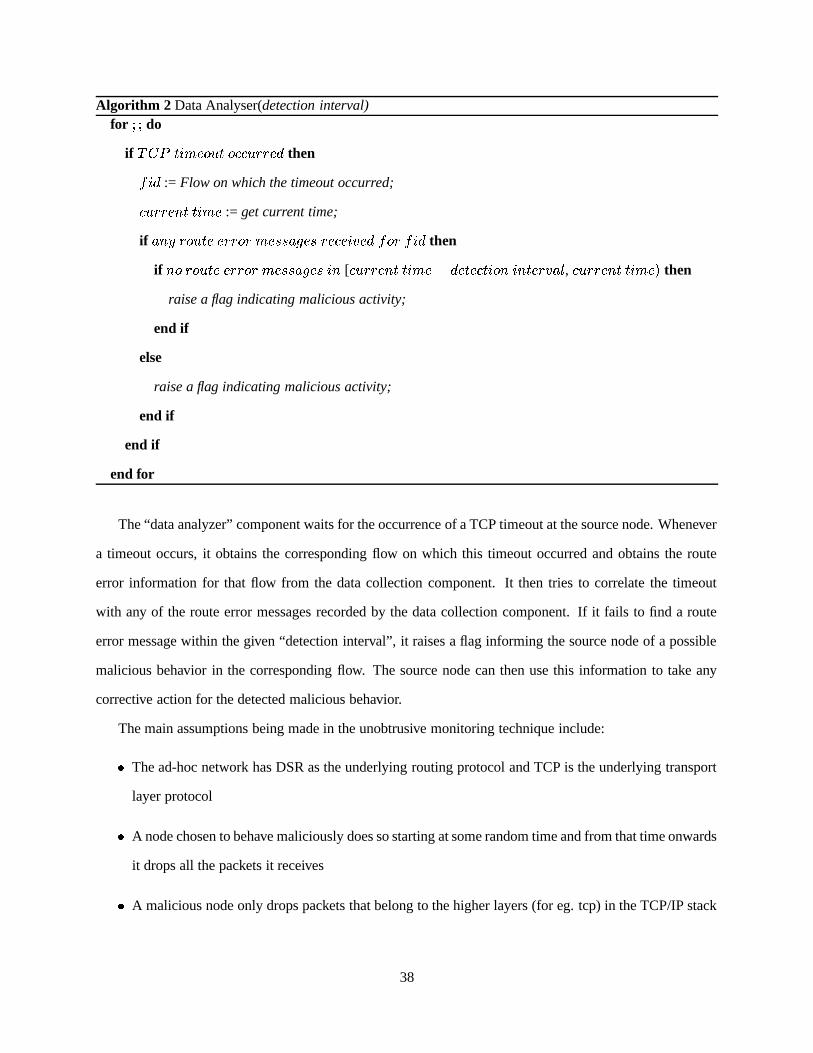
Algorithm 2 Data Analyser(detection interval)for ��� do
if ����� �7!8+,� �� � ��� �6 ���.� $ then% !#$ := Flow on which the timeout occurred;
�&'����� ()�)�*!#+,� := get current time;
if �/(������'�<� � ������� +,�1�����.�������.� ����!#"�� $ % ��� % !#$ then
if ( � ���� ��� ���������2+,�1�����.�����0!8( [ �6'���.� ()�)�*!8+,�:9;$������ �6�*!*��(=!8()������"/��3 , �6 ���.��()� �7!8+,��� then
raise a flag indicating malicious activity;
end if
else
raise a flag indicating malicious activity;
end if
end if
end for
The “data analyzer” component waits for the occurrence of a TCP timeout at the source node. Whenever
a timeout occurs, it obtains the corresponding flow on which this timeout occurred and obtains the route
error information for that flow from the data collection component. It then tries to correlate the timeout
with any of the route error messages recorded by the data collection component. If it fails to find a route
error message within the given “detection interval”, it raises a flag informing the source node of a possible
malicious behavior in the corresponding flow. The source node can then use this information to take any
corrective action for the detected malicious behavior.
The main assumptions being made in the unobtrusive monitoring technique include:
� The ad-hoc network has DSR as the underlying routing protocol and TCP is the underlying transport
layer protocol
� A node chosen to behave maliciously does so starting at some random time and from that time onwards
it drops all the packets it receives
� A malicious node only drops packets that belong to the higher layers (for eg. tcp) in the TCP/IP stack
38

but not the control messages sent out by the DSR agents for route discovery, maintenance etc
� Malicious nodes do not collude with one another
� All the packet drops are either due to malicious packet dropping or due to broken link(s) at some
intermediate node in the source route
� All the mobile nodes have enough memory to store information about the Route Error messages
received within the detection interval
4.3 Example Scenario
The algorithm presented in the previous section can be understood more clearly by looking at the following
example scenario. This example illustrates how the unobtrusive monitoring technique uses information from
different network levels to detect malicious behavior in the network. Specifically, this example illustrates
the use of DSR route error messages and TCP timeout messages to detect malicious packet dropping in the
route from a source to some destination.
In the DSR routing protocol, a node sends a DSR route error message back to the source if it is unable
to deliver the packet to its next hop neighbor as indicated in the source route. This could be due to node
movement which could result in a new network topology and the old route no longer exists or this could be
due to a temporary broken link between the node and its next hop and the node is unable to find an alternate
route to that destination using the routes it had already discovered. A TCP timeout normally occurs when
sender does not receive an acknowledgement within a specific interval. This may happen because the packet
was dropped at an intermediate node due to congestion at that node or the packet’s Time To Live (TTL)
value has expired or by some malicious node trying to disrupt the network or due a broken link at some
intermediate node in the source route or the packet got corrupted during transmission and was dropped
by an intermediate node. But it should be pointed out that the current research assumes that there is no
congestion in the network and hence there will not be any packet drops due to congestion. The distinction
between packet dropping due to congestion and malicious behavior will be studied as part of future research.
The unobtrusive monitoring technique at the source node uses such control information passed between the
source and the destination to detect the presence of malicious nodes in that route.
39
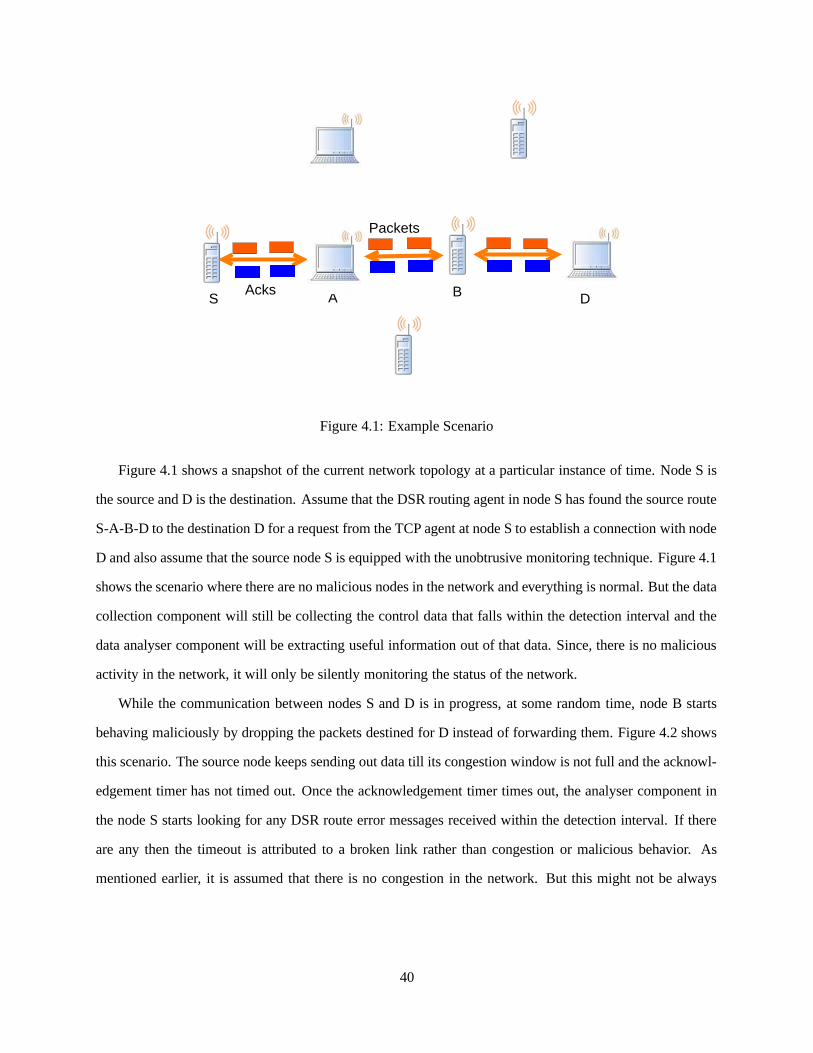
S A DB
Packets
Acks
Figure 4.1: Example Scenario
Figure 4.1 shows a snapshot of the current network topology at a particular instance of time. Node S is
the source and D is the destination. Assume that the DSR routing agent in node S has found the source route
S-A-B-D to the destination D for a request from the TCP agent at node S to establish a connection with node
D and also assume that the source node S is equipped with the unobtrusive monitoring technique. Figure 4.1
shows the scenario where there are no malicious nodes in the network and everything is normal. But the data
collection component will still be collecting the control data that falls within the detection interval and the
data analyser component will be extracting useful information out of that data. Since, there is no malicious
activity in the network, it will only be silently monitoring the status of the network.
While the communication between nodes S and D is in progress, at some random time, node B starts
behaving maliciously by dropping the packets destined for D instead of forwarding them. Figure 4.2 shows
this scenario. The source node keeps sending out data till its congestion window is not full and the acknowl-
edgement timer has not timed out. Once the acknowledgement timer times out, the analyser component in
the node S starts looking for any DSR route error messages received within the detection interval. If there
are any then the timeout is attributed to a broken link rather than congestion or malicious behavior. As
mentioned earlier, it is assumed that there is no congestion in the network. But this might not be always
40

S A DB
Packets
DroppedPackets
Timeout
Figure 4.2: Malicious Packet Dropping
true because depending on the size of the detection interval there could be some stray route error messages
within the interval. So, this would lower our detection efficiency.
But if there are no route error messages within the detection interval, the data analyser component alerts
the node of a potential malicious activity in the source route from the source to the destination. As in the
previous case, this might not always be true and it depends on the size of detection interval. If the detection
interval is smaller, we might lose some genuine route error messages and this would increase our false
positive rate.
So, we can see that the choice of the detection interval plays an important role in the detection efficiency
and false positive rate of the technique. These will be discussed in more detail in the next section and also in
the “Simulation and Results” chapter. Briefly, it can be said that increasing the detection interval might result
in a decrease in the detection efficiency and decreasing the detection interval might result in an increase in
the false positive rate. So, it is important to strike a balance between detection efficiency and false positive
rate by choosing the detection interval appropriately.
Figure 4.3 shows the situation where a false alarm is raised by the data analyser component. In this case,
the destination node D moves out of the transmission range of node B. So, node B fails to deliver the packet
41

S A DB
Packets
RERRDropped
Timeout
RERRX
Figure 4.3: False Alarm
to D and sends out a DSR route error message back to the source S indicating the broken link. But if this
route error message gets lost, then the acknowledgement timer in the source timesout and the data analyser
component looks for any route error messages within the detection interval, finds none and finally raises a
false alarm indicating potential malicious behavior when there is none.
4.4 Detection Interval
Detection interval is the duration within which the data collection component gathers control information
from different levels of the network stack (which is finally fed to the data analyzer component) and purges
any old information that falls outside the interval. As explained earlier, the length of the detection interval
play a vital role in determining the detection efficiency and false positive rate of the unobtrusive monitoring
technique. A lower detection interval might cause genuine route error messages to be purged, raise false
alarms when the TCP timesout and thereby increasing the false positive rate of the technique. Similarly, a
higher detection interval also might have a negative effect on the detection technique. A higher detection
interval might result in failing to detect malicious behavior by associating any TCP timeouts with old route
error messages. Therefore, a higher interval lowers the detection efficiency of the technique. The effect
of detection interval on the detection effectiveness and false positive rate of our unobtrusive monitoring
42

technique will be discussed in more detail in the “Simulation Results” chapter. We will also present the
detection effectiveness and the false positive rate of our technique for different mobility models in that
chapter.
4.5 Thwarting Unobtrusive Monitoring
S A DB
Packets
PacketsDropped
RERR
Figure 4.4: Thwarting Unobtrusive Monitoring
It is possible for an intelligent malicious node to defeat the unobtrusive monitoring technique. If a
malicious node sends back a DSR route error message to the source node for the packets it drops, the source
node will associate the TCP timeouts with the DSR route error messages received and will not be able to
detect the malicious activity going on in the network. Figure 4.4 shows such a scenario. In this case the
malicious node B sends out DSR route error messages to the source node S after dropping packets destined
for node D. So, node S will think of them as genuine timeouts and will fail to detect the malicious behavior.
Also, if a malicious node selectively drops the packets instead of dropping all of them, it will be hard
for the source node to act upon the alarms raised by the data analyser component. For example, if the source
node acts on the alarms only after the number exceeds some threshold value within a specific time interval,
the malicious node could spread out its malicious drops so that the number of drops does not exceed the
threshold within the time interval, making it difficult for the source node to act on them. It is also possible
43

for malicious nodes to collude with one another to launch sophisticated attacks without being detected.
Currently selective packet dropping and colluding malicious nodes are not being taken into consideration
and will be studied as part of future research.
44

CHAPTER FIVE
SIMULATION AND RESULTS
This chapter details the simulation model used for our experiments and provides an analysis of the simulation
results obtained. For our experiments, we have used the Network Simulator 2 (ns 2.1b9a) [27] to simulate
an ad-hoc wireless network running the Dynamic Source Routing protocol. NS (version 2) is an object-
oriented, discrete-event driven network simulator written in C++ and OTcl. NS is useful for simulating a
variety of IP networks. It implements network protocols such as TCP and UPD, traffic source behavior such
as FTP, Telnet, Web, CBR and VBR, router queue management mechanism such as Drop Tail, RED and
CBQ, routing algorithms such as link-state, and more. NS also implements multicasting and some of the
MAC layer protocols for LAN simulations [28], [29].
5.1 Mobility Models
In our simulations, the following mobility models were used to evaluate our unobtrusive monitoring tech-
nique.
� Random Way-Point Model: In this model, a node moves from its current location to a new location by
randomly choosing a direction and speed in which to travel and pauses between changes in direction
and/or speed. This is a memoryless mobility pattern because it retains no knowledge concerning its
past locations and speed values. The current speed and direction of a node is independent of its past
speed and direction. This characteristic can generate unrealistic movements such as sudden stops and
sharp turns [30].
� Gauss-Markov Model: This model was designed to adapt to different levels of randomness. Initially
each node is assigned a current speed and direction. At fixed intervals of time, movement occurs by
updating the speed and direction of each node. Specifically, the value of speed and direction at the n ��
instance is calculated based upon the value of speed and direction at the (n-1) ��
instance. The main
advantages of this model are that it eliminates the sudden stops, sharp turns present in Random way
point mobility model and it is close to being realistic.
45

� Reference Point Group Mobility Model: The Reference Point Group Mobility (RPGM) model repre-
sents the random motion of a group of mobile nodes as well as the random motion of each individual
node within the group. Group movements are based upon the path traveled by a logical center for the
group. The motion of the group center completely characterizes the movement of its corresponding
group of mobile nodes, including their direction and speed. Individual nodes randomly move about
their own pre-defined reference points, whose movements depend on the group movement.
� City Section Mobility Model: In the City Section Mobility Model, the simulation area is a street
network that represents a section of a city where the ad-hoc network exists. The streets and speed
limits on the streets are based on the type of city being simulated. Each MN begins the simulation at a
defined point on some street. A MN then randomly chooses a destination, also represented by a point
on some street. The movement algorithm from the current destination to the new destination locates
a path corresponding to the shortest travel time between the two points; in addition, safe driving
characteristics such as a speed limit and a minimum distance allowed between any two MNs exist.
Upon reaching the destination, the MN pauses for a specified time and then randomly chooses another
destination (i.e., a point on some street) and repeats the process.
For each of these simulations, a network with 50 nodes in a flat 670m X 670m topography was taken
which is very common in current ad-hoc network research and in the simulation examples provided with
ns-2. Each simulation was run for a time period of 150 seconds. In case of random way point networks, the
maximum node speed was set to 20 meters/second to simulate high mobility networks and 5 meters/second
to simulate medium mobility networks. Also, the pause times were set to 5 seconds and 30 seconds to
simulate high and medium mobility networks, respectively.
46

5.2 Communication Patterns
Networks with random way point mobility were generated using the CMU’s TCP/CBR traffic-scenario gen-
erator script and networks with other mobility patterns listed earlier were generated using University of
Bonn’s BonnMotion [31], a mobility scenario generator and analysis tool. A communication pattern speci-
fies the source, destination along with other parameters associated with the connection. In each experiment,
20 different traffic connections were used for the nodes to communicate. The results were taken as the
average of 7 different communication patterns.
5.3 Misbehaving Nodes
The ns-2 simulator was modified to enable particular node(s) to be configured as malicious. The configura-
tion also takes in a time parameter that specifies the time from which that node starts behaving maliciously.
Beginning from that time, the node drops all the packets (non-control packets) that are received at that node
till the end of the simulation. Each network is designed to contain 20 malicious nodes reflecting misbehavior
of 40% of the nodes as suggested in [13]. The number and placement of the malicious nodes ensures that
they will be located along active paths in the network. To determine the effectiveness of our approach, the
percentage of misbehaving nodes was varied from 0% to 40% in 5% increments.
5.4 Performance Metrics
The primary metrics used for evaluating the performance of the proposed unobtrusive monitoring technique
are detection effectiveness and false positive rate.
� Detection Effectiveness: The algorithm used for calculating the “detection effectiveness” of our ap-
proach is as given below:
47

Algorithm 3 Detection Effectiveness(det intval)for � ����- ��� ���7!8+,� ��'��� � do
if � � $. ���7�2+ �/3 !#�6!#�� ���'����� � � $.����� ��� � �����.�1���'��( $.!#( �:������( �� 3 � $��/+,��()� $����� then
recorded++;
� ��� := Source node at which timeout occurred;% !#$ := Flow on which the timed out packet was sent;
��� �*���/( � := Time at which the packet was retransmitted;
����'�<����������� % �� ( $ := ����'�<� � ����������� !*�1�<� atsrcforfidin[retrans - detintval,retrans) �
if ���� ��� ��������� % ��'( $� � % ��3 ��� then
detected++;
end if
end if
end for
return detected/recorded;
Detection effectiveness measures how well the technique does at detecting malicious events or con-
gested behavior. For example, if the node detects each and every instance of a malicious packet drop,
then the detection effectiveness is 100%; but it does not detect any misbehavior, the detection effec-
tiveness is 0%. Identification of malicious behavior is essential. For example, if a node experiences
more than three TCP timeouts and there is no indication of a broken link, then a node in the path is
either misbehaving or is overloaded. Additional information must then be used to clearly identify the
rationale behind the behavior.
� False Positives: The algorithm used for calculating the “false positive rate” of our approach is as given
below:
48

Algorithm 4 False Positive Rate(det intval)for � ����- ��� ���7!8+,� ��'��� � do
if � � !*� $� ���<� ( ��( 9 + �/3 !#�6!#�� � �.� � �1��( � then
goodtimeouts++;
� ��� := Source node at which timeout occurred;% !#$ := Flow on which the timed out packet was sent;
��� �*���/( � := Time at which the packet was retransmitted;
����'�<����������� % �� ( $�� ����'�<��� ����������� !*�1�<���/� �1��� % ��� % !#$:!8(���� �*���/( �29 $���� !#()�*"��/3������ �*���/( � � ;
if ���� ��� ��������� % ��'( $� � % ��3 ��� then
detectbad++;
end if
end if
end for
return detectbad/goodtimeouts;
Reporting a genuine event as malicious is called a false positive. If every reported event is false, then
the node has 100% false positives; on the other hand having no reported false events signifies 0% false
positives. A perfect system will have a detection effectiveness of 100% and 0% false positives, but
this is not always possible. Techniques such as setting alert thresholds can reduce the number of false
positives, but this would also reduce detection effectiveness.
5.5 Detection Interval
Detection interval specifies the duration within which a source node keeps track of all the control messages
(Route Error messages) received at that node. The choice of the detection interval determines the detection
effectiveness and false positive rate of the unobtrusive monitoring technique. Increasing the detection inter-
val might allow unrelated Route error messages to be associated with any TCP time out at the source node
and hence hampering the ability of the technique to detect malicious activity. Having a very small detection
interval also has a negative effect on the false positive rate of the technique. If we have a smaller detection
interval, we might quickly jump to a conclusion about a TCP time out at the source without waiting long
49

enough to include any delayed Route Error message(s) for that flow and hence increasing the false positive
rate of the technique. Also, increasing the detection interval means that a node has to store information for
a longer period of time. If the node is receiving a lot of messages, this can drastically increase the storage
overhead which is a burden on the memory constrained mobile nodes. Therefore, choice of the detection
interval has a very significant impact on the performance metrics and storage overhead of the technique. In
all our simulations, we have experimented with detection intervals ranging from 5 to 50 seconds in 5 second
increments. We observed that at a lower detection interval, we have a high detection effectiveness and also
a high false positive rate. For the detection intervals of 30, 35, and 40 seconds our technique had a good
detection effectiveness with a lower false positive rate. To show how the detection effectiveness and false
positive rate vary with the choice of detection interval, we present the detection effectiveness and false pos-
itive rate for high mobility random way point mobility networks for the following detection intervals: 20,
30, 35, 40, and 50 seconds. For the remaining models, we present the results only for detection intervals of
30, 35, and 40 seconds. The detection effectiveness and false positive rate corresponding to these intervals
for different mobility models are presented in the next section.
5.6 Simulation Results For Different Mobility Models
The different configuration parameters used for generating the required mobility scenarios using BonnMotion[31]
are as given below:
Table 5.1: Configuration parameters used for different mobility models
Mobility Model Speed Pause Time No. of x-blocks No. of y-blocks
Random Way Point (Medium Mobility) 5 (max.) 30 n/a n/aRandom Way Point (High Mobility) 20 (max.) 5 n/a n/a
RPGM (Medium Mobility) 5 (max.) 30 n/a n/aRPGM (High Mobility) 20 (max.) 5 n/a n/a
Gauss Markov 20 (max.) default n/a n/aManhattan Grid 5 (min.) default 50 50
5.6.1 Random Way Point Mobility Networks
In these kind of networks a node chooses a random destination, speed and starts moving towards that des-
tination. Between movements it pauses for some amount of time referred to as “pause time”. To simulate
50

medium mobility networks a maximum node speed of 5 meters/second and a pause time of 30 seconds were
chosen and a maximum speed of 20 meters/second and a pause time of 5 seconds were chosen for high
mobility networks. For high mobility networks, we present the results for detection intervals of 20, 30, 35,
40, and 50 seconds. For medium mobility networks, we present the results for detection intervals of 30, 35,
and 40 seconds. Also, for the metrics considered, the number of malicious nodes is increases from 5% to
40% in 5% increments. The results for the metrics used for these simulations are as given below:
� Detection Efficiency:
0
20
40
60
80
100
120
5 10 15 20 25 30 35 40
Det
ectio
n E
ffect
iven
ess
Percent Malicious Nodes
Detection Effectiveness (rwp_low)
30 sec interval35 sec interval40 sec interval
Figure 5.1: Detection Efficiency – Random Way Point (Medium Mobility)
The detection effectiveness for medium and high mobility networks is as shown in figures 5.1 and
5.2 respectively. From these figures we can see that for both medium and high mobility networks, in-
creasing the detection interval lowers the detection effectiveness. This is because when using a bigger
detection interval, there is a much higher probability of getting unrelated route error messages within
this interval. Also, we can see that the detection effectiveness is better in the case of medium mobility
networks when compared to high mobility ones. Due to higher mobility, the links get broken quite
frequently and there are many route error messages sent out by the nodes in the network. This also
increases the probability of receiving unrelated route error messages within the detection interval at a
51

0
20
40
60
80
100
120
5 10 15 20 25 30 35 40
Det
ectio
n E
ffect
iven
ess
Percent Malicious Nodes
Detection Effectiveness (rwp_high)
20 sec interval30 sec interval35 sec interval40 sec interval50 sec interval
Figure 5.2: Detection Efficiency – Random Way Point (High Mobility)
source node and the source node correlates any TCP timeouts with the received route error message
and thus leads to a decrease in detection effectiveness.
� False Positive Rate:
0
20
40
60
80
100
120
5 10 15 20 25 30 35 40
Fal
se P
ositi
ve R
ate
Percent Malicious Nodes
False Positives (rwp_low)
30 sec interval35 sec interval40 sec interval
Figure 5.3: False Positive Rate – Random Way Point (Medium Mobility)
52

0
20
40
60
80
100
120
5 10 15 20 25 30 35 40
Fal
se P
ositi
ve R
ate
Percent Malicious Nodes
False Positives (rwp_high)
20 sec interval30 sec interval35 sec interval40 sec interval50 sec interval
Figure 5.4: False Positive Rate – Random Way Point (High Mobility)
The false positive rate for medium and high mobility networks is as shown in figures 5.3 and 5.4
respectively. We can see that increasing the detection interval lowers the number of false positives.
This is because, when we have a bigger interval we wait long enough to receive any delayed route error
messages and do not quickly jump to conclusions. As the nodes move faster, the links between the
nodes get broken all the more. So, the route error messages sent out by intermediate nodes might get
dropped before they reach the source node. When the source node timesout it will not find any related
route error messages received by it within the detection interval and might come to a conclusion that
the timeout is due to some malicious behavior in the source route. So, at higher mobility there could
be a higher false positive rate due to the loss of route error messages.
5.6.2 Reference Point Group Mobility
� Detection Efficiency:
The detection effectiveness of the unobtrusive monitoring technique for “Reference Point Group Mo-
bility” is as shown in figures 5.5 and 5.6 for medium and high mobility scenarios respectively. The
analysis provided for the detection effectiveness of “Random Way Point” networks holds true here
also. We can observe that increasing the detection interval decreases the detection effectiveness as in
53
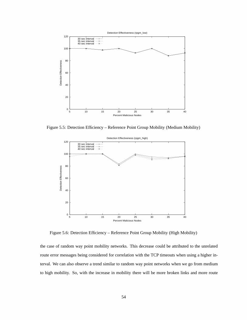
0
20
40
60
80
100
120
5 10 15 20 25 30 35 40
Det
ectio
n E
ffect
iven
ess
Percent Malicious Nodes
Detection Effectiveness (rpgm_low)
30 sec interval35 sec interval40 sec interval
Figure 5.5: Detection Efficiency – Reference Point Group Mobility (Medium Mobility)
0
20
40
60
80
100
120
5 10 15 20 25 30 35 40
Det
ectio
n E
ffect
iven
ess
Percent Malicious Nodes
Detection Effectiveness (rpgm_high)
30 sec interval35 sec interval40 sec interval
Figure 5.6: Detection Efficiency – Reference Point Group Mobility (High Mobility)
the case of random way point mobility networks. This decrease could be attributed to the unrelated
route error messages being considered for correlation with the TCP timeouts when using a higher in-
terval. We can also observe a trend similar to random way point networks when we go from medium
to high mobility. So, with the increase in mobility there will be more broken links and more route
54

0
20
40
60
80
100
120
5 10 15 20 25 30 35 40
Fal
se P
ositi
ve R
ate
Percent Malicious Nodes
False Positives (rpgm_low)
30 sec interval35 sec interval40 sec interval
Figure 5.7: False Positive Rate – Reference Point Group Mobility (Medium Mobility)
0
20
40
60
80
100
120
5 10 15 20 25 30 35 40
Fal
se P
ositi
ve R
ate
Percent Malicious Nodes
False Positives (rpgm_high)
30 sec interval35 sec interval40 sec interval
Figure 5.8: False Positive Rate – Reference Point Group Mobility (High Mobility)
error messages sent out to the source nodes. So, the source node could miss some malicious drop
events by correlating a TCP timeout with one of the many route error messages received by it due
to increased mobility in the network. Also, since the nodes move in groups and with reference to a
leader, there will not be as many broken links as in the case of random way point mobility. So, the
55

chance of getting a stray route error message within the detection interval is much lower in the case of
reference point group mobility when compared to random way point. So, in this case we can expect a
much higher detection efficiency when compared to the random way point mobility model.
� False Positive Rate:
The false positive rate of the unobtrusive monitoring technique for “Reference Point Group Mobility”
is as shown in figures 5.7 and 5.8 for medium and high mobility scenarios respectively. In this case
also, the increase in mobility affects the false positive rate of the technique. It is more likely for
the route error messages to be dropped by some intermediate nodes before they actually reach the
intended source node. So, the source node, which is unaware of the loss of route error messages,
attributes any genuine timeouts due to broken links as being malicious. This leads to an increase in
the false positive rate at higher mobility. Also, in the case of reference point group mobility, there
will be fewer broken links when compared to the random wap point mobility due to the nature of
movement of the nodes. So, misdetecting a single normal timeout as malicious will greatly affect the
false positive rate.
5.6.3 Gauss-Markov
In this model also, the nodes move about at a maximum speed of 20 m/s. So, this represents a high mobility
Gauss-Markov model. We can observe a similar effect of the detection interval on the detection effectiveness
and false positive rate as we have seen in the previous mobility models.
� Detection Efficiency:
Figure 5.9 shows the detection effectiveness of the technique for “Gauss Markov” mobility model.
Here also, the detection effectiveness decreases with increase in the detection interval agreeing with
the previous scenarios. As mentioned earlier, this is a more realistic mobility model when compared
with the random way point model where nodes choose a random destination, speed and starting mov-
ing toward the destination. So, when we compare the detection effectiveness of this model with the
high mobility random way point model, we can see that the Gauss-Markov model exhibits a slightly
better detection effectiveness when compared to the random way point model. This could be due
56

0
20
40
60
80
100
120
5 10 15 20 25 30 35 40
Det
ectio
n E
ffect
iven
ess
Percent Malicious Nodes
Detection Effectiveness (gmarkov)
30 sec interval35 sec interval40 sec interval
Figure 5.9: Detection Efficiency – Gauss Markov
0
20
40
60
80
100
120
5 10 15 20 25 30 35 40
Fal
se P
ositi
ve R
ate
Percent Malicious Nodes
False Positives (gmarkov)
30 sec interval35 sec interval40 sec interval
Figure 5.10: False Positive Rate – Gauss Markov
to the more realistic movement of the nodes in this model. Because of a more realistic mobility, the
chances of getting an unrelated route error messages is lower in the case of Gauss-Markov model when
compared to the Random Way Point mobility model which leads to a better detection effectiveness.
57

� False Positive Rate:
Figure 5.10 shows the false positive rate of the technique for “Gauss Markov” mobility model. The
results agree with the previous scenarios as the false positive rate decreases with increase in detection
interval. Also, when we compare this result with that of random way point mobility networks, we
can observe that Gauss-Markov has a slightly lower false positive rate. This can again be attributed
to the more realistic motion in the case of Gauss-Markov model. We speculate that the number of
route error messages dropped is more in the case of random way point mobility when compared to
Gauss-Markov mobility which leads to a lower false positive rate for Gauss-Markov mobility model.
5.6.4 Manhattan Grid
� Detection Efficiency:
0
20
40
60
80
100
120
5 10 15 20 25 30 35 40
Det
ectio
n E
ffect
iven
ess
Percent Malicious Nodes
Detection Effectiveness (mgrid)
30 sec interval35 sec interval40 sec interval
Figure 5.11: Detection Efficiency – Manhattan Grid
Figure 5.11 shows the detection effectiveness of the technique for “Manhattan Grid” mobility model.
Here also, the detection effectiveness decreases with increase in the detection interval agreeing with
the previous scenarios. This mobility model can be thought of as a special case of random way
point mobility model with the nodes choosing a random destination either in the horizontal or vertical
directions. This mobility model demonstrates a detection effectiveness slightly better than the high
58

0
20
40
60
80
100
120
5 10 15 20 25 30 35 40
Fal
se P
ositi
ve R
ate
Percent Malicious Nodes
False Positives (mgrid)
30 sec interval35 sec interval40 sec interval
Figure 5.12: False Positive Rate – Manhattan Grid
mobility random way point mobility networks. Again as in the case of Gauss-Markov model, this
could be due to the more restricted movement of the nodes in the network which leads to slightly
lesser number of broken links and subsequently lowering the chance of getting a stray route error
message.
� False Positive Rate:
Figure 5.12 shows the false positive rate for the “Manhattan Grid” mobility model. The results agree
with the previous scenarios as the false positive rate decreases with increase in detection interval.
Also, this model has a false positive rate quite similar to that of high mobility random way point
networks.
In this chapter, we have seen the detection effectiveness and the false positive rates of our technique
for different mobility models. In all the mobility models we have observed that the choice of the detection
interval plays an important role in determining the detection effectiveness and false positive rate of the
technique. Having a higher detection interval leads to a much better false positive rate and a much lower
detection effectiveness. Similarly, lowering the detection interval increases the detection effectiveness and
at the same time leads to a much higher false positive rate. So, we need to choose a detection interval
59

which enables the technique to exhibit a good detection efficiency while keeping the false positive rate
at a reasonable value. We varied the detection interval from 5 to 50 seconds in 5 second increments and
observed that detection intervals in the range 30 to 40 seconds provide a good detection effectiveness while
maintaining the false positives at a reasonable value.
60

CHAPTER SIX
CONCLUSIONS AND FUTURE WORK
Mobile ad-hoc networks have several advantages over traditional wireless networks including ease of de-
ployment, speed of deployment, and decreased dependence on a fixed infrastructure. Mobile ad-hoc net-
works constitute an emerging wireless networking technology for future mobile communications. However,
unless the networks can be secured against malicious activity, their usefulness may be stifled. The task of
finding good solutions for these security challenges prevalent in ad-hoc wireless networks will play a critical
role in achieving the eventual success and potential of mobile ad-hoc network technology.
To help protect ad-hoc wireless networks from malicious nodes, we developed an unobtrusive monitor-
ing technique to detect malicious behavior in the network by gathering information from different network
levels with out relying on node cooperation. Unlike some other proposed methods, this technique is easy to
deploy, since it only requires modification to a single device, and it does not require any additional infras-
tructure or security associations.
Simulation results show that this technique has good detection effectiveness across a wide variety of
network mobility models. The detection effectiveness tends to decrease when the network is highly loaded,
when there is a long distance between neighboring nodes, or when the nodes are highly mobile. These
situations are problematic for the network in general, since they cause increase in route maintenance and
a decrease in packet transmission success. This technique also maintains low false positive rate in all the
different scenarios considered.
In the future, we would like to extend the unobtrusive monitoring technique to distinguish packet drops
arising due to congestion and malicious behavior. We also plan to investigate the use of this technique with
other ad-hoc routing protocols, such as AODV, TORA, and with other types of networks, such as hybrid
wired-wireless networks and traditional wired networks. We would also like to extend this technique to
handle partial packet dropping and also to detect any sophisticated attacks launched by colluding nodes.
61

BIBLIOGRAPHY
[1] C. E. Perkins. Ad Hoc Networking. Addison-Wesley Professional, first edition, 2000.
[2] D. B. Johnson, D. A. Maltz, Y. Hu, and J. G. Jetcheva. The dynamic source routing protocol for mobile
ad hoc networks (DSR). Internet draft, February 2002. draft-ietf-manet-dsr-08.txt.
[3] S. R. Medidi, M. Medidi, and S. Gavini. Detecting packet-dropping faults in mobile ad-hoc networks.
In Proceedings of The Thirty-Seventh Asilomar Conference on Signals, Systems & Computers, pages
1708–1712, November 2003.
[4] S. Medidi, M. Medidi, S. Gavini, and R. Griswold. Detecting packet mishandling in manets. In
Security and Management, pages 159–162, 2004.
[5] A. S. Tanenbaum. Computer Networks. Prentice Hall, third edition.
[6] J. F. Kurose and K. W. Ross. Computer Networking: A Top-Down Approach Featuring the Internet.
Addison-Wesley, second edition, 2002.
[7] C. E. Perkins and P. Bhagwat. Highly dynamic destination-sequenced distance-vector routing (DSDV)
for mobile computers. In ACM SIGCOMM’94 Conference on Communications Architectures, Proto-
cols and Applications, pages 234–244, 1994.
[8] C. E. Perkins, E. M. Belding-Royer, and S. R. Das. Ad hoc on-demand distance vector (AODV)
routing. Internet draft, February 2003. draft-ietf-manet-aodv-13.txt.
[9] H. Bakht. Understanding mobile ad-hoc networks. Online. http://www.computingunplugged.com.
[10] H. Yang, H. Luo, F. Ye, S. Lu, and L. Zhang. Security in mobile ad hoc networks: challenges and
solutions. IEEE Wireless Communications, 11(1):38–47, March-April 2002.
[11] R. Griswold and S. Medidi. Malicious node detection in ad-hoc wireless networks. In Proceedings of
SPIE AeroSense, Digital Wireless Communications V, April 2003.
62

[12] S. Buchegger and J. Le Boudec. Nodes bearing grudges: Towards routing security, fairness, and
robustness in mobile ad hoc networks. In Proceedings of the Parallel, Distributed and Network-based
Processing, pages 403–410, January 2002.
[13] S. Marti, T. J. Giuli, K. Lai, and M. Baker. Mitigating routing misbehavior in mobile ad hoc networks.
In Proceedings of the Mobile Computing and Networking, pages 255–265, 2000.
[14] R. Griswold. Malicious node detection in ad hoc wireless networks. Master’s thesis, Washington State
University, Pullman, 2003.
[15] K. Park and H. Lee. On the effectiveness of probabilistic packet marking for ip traceback under denial
of service attack. In Proceedings of the INFOCOM, volume 1, pages 338–347, April 2001.
[16] P. Ferguson and D. Senie. RFC 2267: Network Ingress Filtering: Defeating Denial of Service Attacks
which employ IP Source Address Spoofing. Internet standard, January 1998.
[17] Y. Zhang and W. Lee. Intrusion detection in wireless ad-hoc networks. In Mobile Computing and
Networking, pages 275–283, August 2000.
[18] S. Savage, D. Wetherall, A. Karlin, and T. Anderson. Practical network support for ip traceback. In
Proceedings of the conference on Applications, Technologies, Architectures, and Protocols for Com-
puter Communication (SIGCOMM), pages 295–306. ACM Press, 2000.
[19] V. Jacobson. Traceroute. Computer software. Available from ftp://ftp.ee.lbl.gov/traceroute.tar.gz.
[20] J. B. Postel. RFC 768: User Datagram Protocol. Internet standard, August 1980.
[21] D. Maughan, M. Schertler, M. Schneider, and J. Turner. RFC 2408: Internet Security Association and
Key Management Protocol (ISAKMP). Internet standard, November 1998.
[22] S. Kent and R. Atkinson. RFC 2401: Security Architecture for the Internet Protocol. Internet standard,
November 1998.
[23] R. Thayer, N. Doraswamy, and R. Glenn. RFC 2411: IP Security Document Roadmap. Internet
standard, November 1998.
63

[24] P. Zimmermann. The Official PGP User’s Guide. MIT Press, June 1996.
[25] W. Koch et al. GNU Privacy Guard. Computer software. Available from http://www.gnupg.org/.
[26] F. Stajano and R. Anderson. The resurrecting duckling: Security issues for ad-hoc wireless networks.
In Proceedings of the International Workshop on Security Protocols, pages 172–194, April 1999.
[27] University of Southern California Information Sciences Institute (USC/ISI). The network simulator -
ns-2. Computer software. Available from http://www.isi.edu/nsnam/ns/.
[28] WPI. NS by Example. Online. Accessed from http://nile.wpi.edu/NS/.
[29] M. Greis. Tutorial for the Network Simulator “ns”. Online. Accessed from
http://www.isi.edu/nsnam/ns/tutorial/.
[30] T. Camp, J. Boleng, and V. Davies. A survey of mobility models for ad hoc network research. In
Wireless Communication & Mobile Computing, pages 483–502, 2002.
[31] BonnMotion. University of bonn. Computer software. Available from http://web.informatik.uni-
bonn.de/IV/Mitarbeiter/dewaal/BonnMotion/bonnmotion-1.2b.zip.
64