Detecting Credit Card Fraud using Periodic Features

Alejandro Correa Bahnsen, Djamila Aouada, Aleksandar Stojanovic and Bjorn OtterstenInterdisciplinary Centre for Security, Reliability and Trust

University of Luxembourg, LuxembourgEmail: al.bahnsen@gmail.com, djamila.aouada@uni.lu, aleksandar.stojanovic@rwth-aachen.de, bjorn.ottersten@uni.lu

Abstract—When constructing a credit card fraud detectionmodel, it is very important to extract the right features fromtransactional data. This is usually done by aggregating thetransactions in order to observe the spending behavioral patternsof the customers. In this paper we propose to create a new set offeatures based on analyzing the periodic behavior of the time ofa transaction using the von Mises distribution. Using a real creditcard fraud dataset provided by a large European card processingcompany, we compare state-of-the-art credit card fraud detectionmodels, and evaluate how the different sets of features havean impact on the results. By including the proposed periodicfeatures into the methods, the results show an average increasein savings of 13%. The aforementioned card processing companyis currently incorporating the methodology proposed in this paperinto their fraud detection system.

Keywords—Fraud detection; von Mises distribution; Cost-sensitive learning

I. INTRODUCTION

Credit card fraud has been a growing problem worldwide.During 2012 the total level of fraud reached 1.33 billionEuros in the Single Euro Payments Area, which representsan increase of 14.8% compared with 2011 [1]. Moreover,payments across non traditional channels (mobile, internet,...) accounted for 60% of the fraud, whereas it was 46%in 2008. This opens new challenges as new fraud patternsemerge, and current fraud detection systems are less successfulin preventing these frauds. Furthermore, fraudsters constantlychange their strategies to avoid being detected, something thatmakes traditional fraud detection tools, such as expert rules,inadequate [2].

The use of machine learning in fraud detection has been aninteresting topic in recent years. Different detection systemsthat are based on machine learning techniques have beensuccessfully used for this problem, in particular: neural net-works [3], Bayesian learning [4], artificial immune systems[5], hybrid models [6], support vector machines [7], peergroup analysis [8], online learning [9] and social networkanalysis [2].

When constructing a credit card fraud detection model, itis very important to use those features that allow accurate clas-sification. Typical models only use raw transactional features,such as time, amount, place of the transaction. However, theseapproaches do not take into account the spending behaviorof the customer, which is expected to help discover fraudpatterns [5]. A standard way to include these behavioralspending patterns is proposed in [10], where Whitrow et al.proposed a transaction aggregation strategy in order to take intoaccount a customer spending behavior. The computation of theaggregated features consists in grouping the transactions made

during the last given number of hours, first by card or accountnumber, then by transaction type, merchant group, country orother, followed by calculating the number of transactions orthe total amount spent on those transactions.

In this paper, we propose a new set of features based onanalyzing the time of a transaction. The logic behind it is thata customer is expected to make transactions at similar hours.We, hence, propose a new method for creating features basedon the periodic behavior of a transaction time, using the vonMises distribution [11]. In particular, these new time featuresshould estimate if the time of a new transaction is within theconfidence interval of the previous transaction time.

Furthermore, using a real credit card fraud dataset providedby a large European card processing company, we compare thedifferent sets of features (raw, aggregated and periodic), usingtwo kinds of classification algorithms; cost-insensitive [12] andexample-dependent cost-sensitive [13]. The results show anaverage increase in the savings of 13% by using the proposedperiodic features. Additionally, the outcome of this paper isbeing currently used to implement a state-of-the-art frauddetection system, that will help to combat fraud once theimplementation stage is finished.

The remainder of the paper is organized as follows. InSection 2, we discuss current approaches to create the fea-tures used in fraud detection models. Then, in Section 3, wepresent our proposed methodology to create periodic features.Afterwards, the experimental setup and the results are given inSections 4 and 5. Finally, conclusions and discussions of thepaper are presented in Section 6.

II. TRANSACTION AGGREGATION STRATEGIES

When constructing a credit card fraud detection algorithm,the initial set of features (raw features) include informationregarding individual transactions. It is observed throughout theliterature, that regardless of the study, the set of raw featuresis quite similar. This is because the data collected during acredit card transaction must comply with international financialreporting standards. In TABLE I, the typical credit card frauddetection raw features are summarized.

Several studies use only the raw features in carrying theiranalysis [3], [4]. However, as noted in [14], a single transactioninformation is not sufficient to detect a fraudulent transaction,since using only the raw features leaves behind importantinformation such as the consumer spending behavior, whichis usually used by commercial fraud detection systems [10].

To deal with this, in [5], a new set of features wereproposed such that the information of the last transaction madewith the same credit card is also used to make a prediction.

TABLE I. SUMMARY OF TYPICAL RAW CREDIT CARD FRAUDDETECTION FEATURES

Attribute name DescriptionTransaction ID Transaction identification numberTime Date and time of the transactionAccount number Identification number of the customerCard number Identification of the credit cardTransaction type ie. Internet, ATM, POS, ...Entry mode ie. Chip and pin, magnetic stripe, ...Amount Amount of the transaction in EurosMerchant code Identification of the merchant typeMerchant group Merchant group identificationCountry Country of trxCountry 2 Country of residenceType of card ie. Visa debit, Mastercard, American Express...Gender Gender of the card holderAge Card holder ageBank Issuer bank of the card

The objective, is to be able to detect very dissimilar continuoustransactions within the purchases of a customer. The new setof features include: time since the last transaction, previousamount of the transaction, previous country of the transaction.Nevertheless, these features do not take into account consumerbehavior other than the last transaction made by a client, thisleads to having an incomplete profile of customers.

A more compressive way to take into account a customerspending behavior is to derive some features using a trans-action aggregation strategy. This methodology was initiallyproposed in [10]. The derivation of the aggregation featuresconsists in grouping the transactions made during the last givennumber of hours, first by card or account number, then bytransaction type, merchant group, country or other, followedby calculating the number of transactions or the total amountspent on those transactions. This methodology has been usedby a number of studies [7]–[9], [15]–[18].

When aggregating a customer transactions, there is animportant question on how much to accumulate, in the sensethat the marginal value of new information may diminish astime passes. [10] discuss that aggregating 101 transactionsis not likely to be more informative than aggregating 100transactions. Indeed, when time passes, information lose theirvalue, in the sense that a customer spending patterns arenot expected to remain constant over the years. In particular,Whitrow et al. define a fixed time frame to be 24, 60 or 168hours.

Let S be a set of N transactions, i.e., N = |S|,where each transaction is represented by the feature vectorxi = [x1i , x

2i , ..., x

ki ], where k is the number of features, and

labelled using the class label yi ∈ {0, 1}. Then, the processof aggregating features consists in selecting those transactionsthat were made in the previous tp hours, for each transactioni in the dataset S,

Sagg ≡ TRXagg(S, i, tp) ={xamtl

∣∣∣∣ (xidl = xidi)∧

(hours(xtimei , xtimel ) < tp

)}Nl=1

, (1)

where TRXagg is a function that creates a subset of Sassociated with a transaction i with respect to the time frametp, N = |S|, | · | being the cardinality of a set, xtimei is thetime of transaction i, xamti is the amount of transaction i,xidi the customer identification number of transaction i, and

TABLE II. EXAMPLE CALCULATION OF AGGREGATED FEATURES.WHERE, xa1

i IS THE NUMBER OF TRANSACTIONS IN THE LAST 24 HOURSAND xa2

i IS THE SUM OF THE TRANSACTIONS AMOUNTS IN THE SAMETIME PERIOD.

Raw features Agg. featuresTrxId CardId Time Type Country Amt. xa1i xa2i

1 1 01/01 18:20 POS Lux 250 0 02 1 01/01 20:35 POS Lux 400 1 2503 1 01/01 22:30 ATM Lux 250 2 6504 1 02/01 00:50 POS Ger 50 3 9005 1 02/01 19:18 POS Ger 100 3 7006 1 02/01 23:45 POS Ger 150 2 1507 1 03/01 06:00 POS Lux 10 3 400

hours(t1, t2) is a function that calculates the number of hoursbetween the times t1 and t2. Afterwards the feature numberof transactions and amount of transactions in the last tp hoursare calculated as:

xa1i = |Sagg|, (2)

andxa2i =

∑xamt∈Sagg

xamt, (3)

respectively.

To further clarify how the aggregated features are calcu-lated we show an example. Consider a set of transactions madeby a client between the first and third of January of 2015, asshown in TABLE II. Then we estimate the aggregated features(xa1i and xa2i ) by setting tp = 24 hours. Moreover, the totalnumber of aggregated features can grow quite quickly, as tpcan have several values, and the combination of combinationcriteria can be quite large as well. In [17], we used a totalof 280 aggregated features. In particular we set the differentvalues of tp to: 1, 3, 6, 12, 18, 24, 72 and 168 hours. Thencalculate the aggregated features using (1) with the followinggrouping criteria: country, type of transaction, entry mode,merchant code and merchant group.

III. PROPOSED PERIODIC FEATURES

When using the aggregated features, there is still someinformation that is not completely captured by those features.In particular we are interested in analyzing the time of thetransaction. The logic behind this, is that a customer isexpected to make transactions at similar hours. The issue whendealing with the time of the transaction, specifically, whenanalyzing a feature such as the mean of transactions time, isthat it is easy to make the mistake of using the arithmeticmean. Indeed, the arithmetic mean is not a correct way toaverage time because, as shown in Fig. 1, it does not take intoaccount the periodic behavior of the time feature. For example,the arithmetic mean of transaction time of four transactionsmade at 2:00, 3:00, 22:00 and 23:00 is 12:30, which is counterintuitive since no transaction was made close to that time.

We propose to overcome this limitation by modeling thetime of the transaction as a periodic variable, in particular usingthe von Mises distribution [11]. The von Mises distribution,also known as the periodic normal distribution, is a distributionof a wrapped normal distributed variable across a circle.The von Mises probability distribution of a set of examples

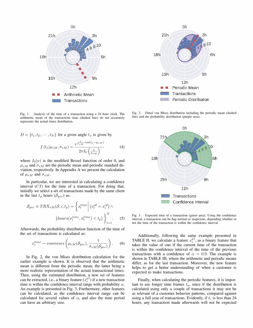
Fig. 1. Analysis of the time of a transaction using a 24 hour clock. Thearithmetic mean of the transactions time (dashed line) do not accuratelyrepresents the actual times distribution.

D = {t1, t2, · · · , tN} for a given angle tx is given by

f (tx|µvM , σvM ) =e

1σvM

cos(tx−µvM )

2πI0

(1

σvM

) (4)

where I0(κ) is the modified Bessel function of order 0, andµvM and σvM are the periodic mean and periodic standard de-viation, respectively. In Appendix A we present the calculationof µvM and σvM .

In particular, we are interested in calculating a confidenceinterval (CI) for the time of a transaction. For doing that,initially we select a set of transactions made by the same clientin the last tp hours (Sper) as:

Sper ≡ TRXvM (S, i, tp) ={xtimel

∣∣∣∣ (xidl = xidi)∧

(hours(xtimei , xtimel ) < tp

)}Nl=1

. (5)

Afterwards, the probability distribution function of the time ofthe set of transactions is calculated as:

xtimei ∼ vonmises(µvM (Sper),

1

σvM (Sper)

). (6)

In Fig. 2, the von Mises distribution calculation for theearlier example is shown. It is observed that the arithmeticmean is different from the periodic mean, the latter being amore realistic representation of the actual transactional times.Then, using the estimated distribution, a new set of featurescan be extracted, i.e., a binary feature (xp1i ) if a new transactiontime is within the confidence interval range with probability α.An example is presented in Fig. 3. Furthermore, other featurescan be calculated, as the confidence interval range can becalculated for several values of α, and also the time periodcan have an arbitrary size.

Fig. 2. Fitted von Mises distribution including the periodic mean (dashedline) and the probability distribution (purple area).

Fig. 3. Expected time of a transaction (green area). Using the confidenceinterval, a transaction can be flag normal or suspicious, depending whether ornot the time of the transaction is within the confidence interval.

Additionally, following the same example presented inTABLE II, we calculate a feature xp1i , as a binary feature thattakes the value of one if the current time of the transactionis within the confidence interval of the time of the previoustransactions with a confidence of α = 0.9. The example isshown in TABLE III, where the arithmetic and periodic meansdiffer, as for the last transaction. Moreover, the new featurehelps to get a better understanding of when a customer isexpected to make transactions.

Finally, when calculating the periodic features, it is impor-tant to use longer time frames tp, since if the distribution iscalculated using only a couple of transactions it may not beas relevant of a customer behavior patterns, compared againstusing a full year of transactions. Evidently, if tc is less than 24hours, any transaction made afterwards will not be expected

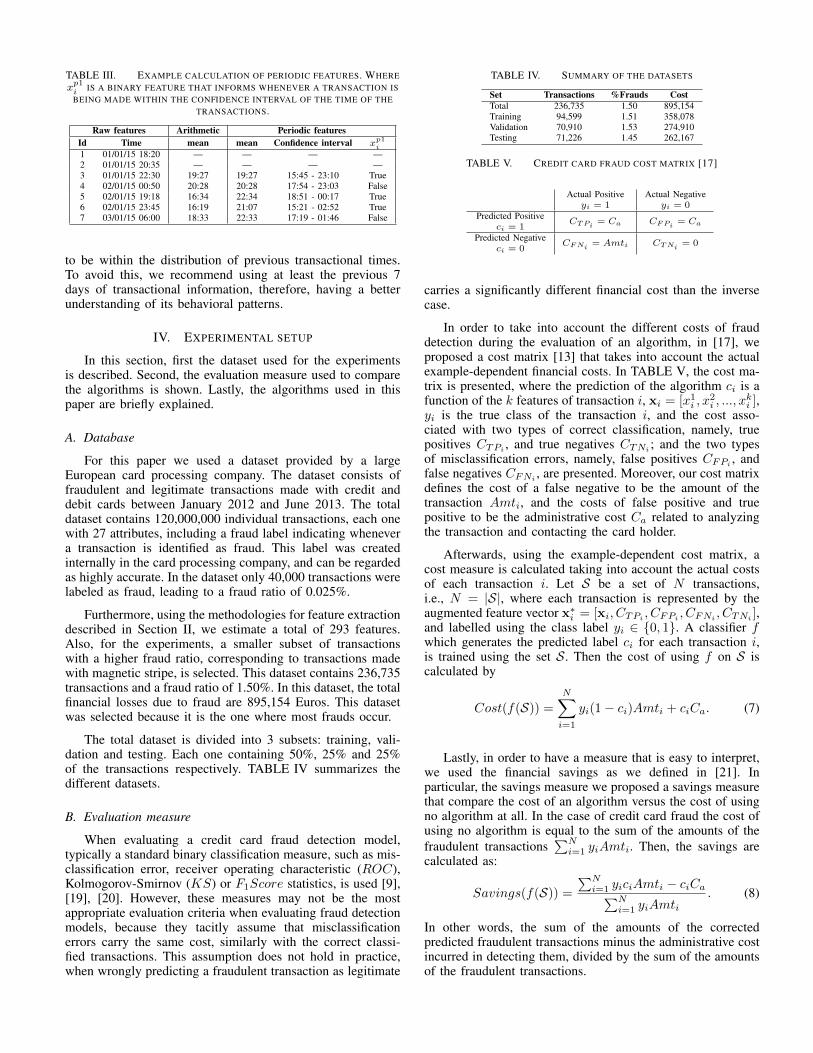
TABLE III. EXAMPLE CALCULATION OF PERIODIC FEATURES. WHERExp1i IS A BINARY FEATURE THAT INFORMS WHENEVER A TRANSACTION ISBEING MADE WITHIN THE CONFIDENCE INTERVAL OF THE TIME OF THE

TRANSACTIONS.

Raw features Arithmetic Periodic featuresId Time mean mean Confidence interval xp1

i1 01/01/15 18:20 — — — —2 01/01/15 20:35 — — — —3 01/01/15 22:30 19:27 19:27 15:45 - 23:10 True4 02/01/15 00:50 20:28 20:28 17:54 - 23:03 False5 02/01/15 19:18 16:34 22:34 18:51 - 00:17 True6 02/01/15 23:45 16:19 21:07 15:21 - 02:52 True7 03/01/15 06:00 18:33 22:33 17:19 - 01:46 False

to be within the distribution of previous transactional times.To avoid this, we recommend using at least the previous 7days of transactional information, therefore, having a betterunderstanding of its behavioral patterns.

IV. EXPERIMENTAL SETUP

In this section, first the dataset used for the experimentsis described. Second, the evaluation measure used to comparethe algorithms is shown. Lastly, the algorithms used in thispaper are briefly explained.

A. Database

For this paper we used a dataset provided by a largeEuropean card processing company. The dataset consists offraudulent and legitimate transactions made with credit anddebit cards between January 2012 and June 2013. The totaldataset contains 120,000,000 individual transactions, each onewith 27 attributes, including a fraud label indicating whenevera transaction is identified as fraud. This label was createdinternally in the card processing company, and can be regardedas highly accurate. In the dataset only 40,000 transactions werelabeled as fraud, leading to a fraud ratio of 0.025%.

Furthermore, using the methodologies for feature extractiondescribed in Section II, we estimate a total of 293 features.Also, for the experiments, a smaller subset of transactionswith a higher fraud ratio, corresponding to transactions madewith magnetic stripe, is selected. This dataset contains 236,735transactions and a fraud ratio of 1.50%. In this dataset, the totalfinancial losses due to fraud are 895,154 Euros. This datasetwas selected because it is the one where most frauds occur.

The total dataset is divided into 3 subsets: training, vali-dation and testing. Each one containing 50%, 25% and 25%of the transactions respectively. TABLE IV summarizes thedifferent datasets.

B. Evaluation measure

When evaluating a credit card fraud detection model,typically a standard binary classification measure, such as mis-classification error, receiver operating characteristic (ROC),Kolmogorov-Smirnov (KS) or F1Score statistics, is used [9],[19], [20]. However, these measures may not be the mostappropriate evaluation criteria when evaluating fraud detectionmodels, because they tacitly assume that misclassificationerrors carry the same cost, similarly with the correct classi-fied transactions. This assumption does not hold in practice,when wrongly predicting a fraudulent transaction as legitimate

TABLE IV. SUMMARY OF THE DATASETS

Set Transactions %Frauds CostTotal 236,735 1.50 895,154Training 94,599 1.51 358,078Validation 70,910 1.53 274,910Testing 71,226 1.45 262,167

TABLE V. CREDIT CARD FRAUD COST MATRIX [17]

Actual Positive Actual Negativeyi = 1 yi = 0

Predicted PositiveCTPi = Ca CFPi = Caci = 1

Predicted NegativeCFNi = Amti CTNi = 0

ci = 0

carries a significantly different financial cost than the inversecase.

In order to take into account the different costs of frauddetection during the evaluation of an algorithm, in [17], weproposed a cost matrix [13] that takes into account the actualexample-dependent financial costs. In TABLE V, the cost ma-trix is presented, where the prediction of the algorithm ci is afunction of the k features of transaction i, xi = [x1i , x

2i , ..., x

ki ],

yi is the true class of the transaction i, and the cost asso-ciated with two types of correct classification, namely, truepositives CTPi , and true negatives CTNi ; and the two typesof misclassification errors, namely, false positives CFPi , andfalse negatives CFNi , are presented. Moreover, our cost matrixdefines the cost of a false negative to be the amount of thetransaction Amti, and the costs of false positive and truepositive to be the administrative cost Ca related to analyzingthe transaction and contacting the card holder.

Afterwards, using the example-dependent cost matrix, acost measure is calculated taking into account the actual costsof each transaction i. Let S be a set of N transactions,i.e., N = |S|, where each transaction is represented by theaugmented feature vector x∗i = [xi, CTPi , CFPi , CFNi , CTNi ],and labelled using the class label yi ∈ {0, 1}. A classifier fwhich generates the predicted label ci for each transaction i,is trained using the set S. Then the cost of using f on S iscalculated by

Cost(f(S)) =N∑i=1

yi(1− ci)Amti + ciCa. (7)

Lastly, in order to have a measure that is easy to interpret,we used the financial savings as we defined in [21]. Inparticular, the savings measure we proposed a savings measurethat compare the cost of an algorithm versus the cost of usingno algorithm at all. In the case of credit card fraud the cost ofusing no algorithm is equal to the sum of the amounts of thefraudulent transactions

∑Ni=1 yiAmti. Then, the savings are

calculated as:

Savings(f(S)) =∑Ni=1 yiciAmti − ciCa∑N

i=1 yiAmti. (8)

In other words, the sum of the amounts of the correctedpredicted fraudulent transactions minus the administrative costincurred in detecting them, divided by the sum of the amountsof the fraudulent transactions.

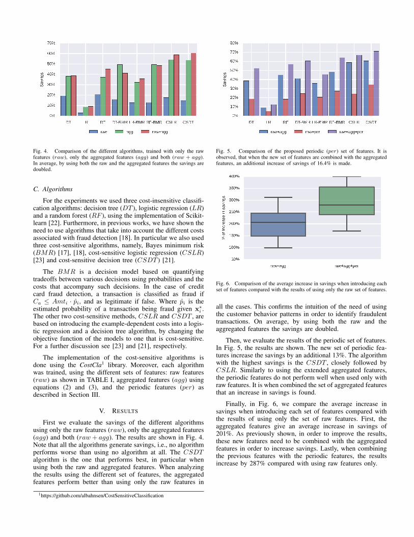
Fig. 4. Comparison of the different algorithms, trained with only the rawfeatures (raw), only the aggregated features (agg) and both (raw + agg).In average, by using both the raw and the aggregated features the savings aredoubled.

C. Algorithms

For the experiments we used three cost-insensitive classifi-cation algorithms: decision tree (DT ), logistic regression (LR)and a random forest (RF ), using the implementation of Scikit-learn [22]. Furthermore, in previous works, we have shown theneed to use algorithms that take into account the different costsassociated with fraud detection [18]. In particular we also usedthree cost-sensitive algorithms, namely, Bayes minimum risk(BMR) [17], [18], cost-sensitive logistic regression (CSLR)[23] and cost-sensitive decision tree (CSDT ) [21].

The BMR is a decision model based on quantifyingtradeoffs between various decisions using probabilities and thecosts that accompany such decisions. In the case of creditcard fraud detection, a transaction is classified as fraud ifCa ≤ Amti · pi, and as legitimate if false. Where pi is theestimated probability of a transaction being fraud given x∗i .The other two cost-sensitive methods, CSLR and CSDT , arebased on introducing the example-dependent costs into a logis-tic regression and a decision tree algorithm, by changing theobjective function of the models to one that is cost-sensitive.For a further discussion see [23] and [21], respectively.

The implementation of the cost-sensitive algorithms isdone using the CostCla1 library. Moreover, each algorithmwas trained, using the different sets of features: raw features(raw) as shown in TABLE I, aggregated features (agg) usingequations (2) and (3), and the periodic features (per) asdescribed in Section III.

V. RESULTS

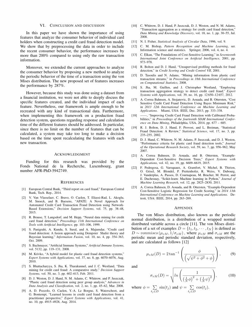
First we evaluate the savings of the different algorithmsusing only the raw features (raw), only the aggregated features(agg) and both (raw+ agg). The results are shown in Fig. 4.Note that all the algorithms generate savings, i.e., no algorithmperforms worse than using no algorithm at all. The CSDTalgorithm is the one that performs best, in particular whenusing both the raw and aggregated features. When analyzingthe results using the different set of features, the aggregatedfeatures perform better than using only the raw features in

1https://github.com/albahnsen/CostSensitiveClassification

Fig. 5. Comparison of the proposed periodic (per) set of features. It isobserved, that when the new set of features are combined with the aggregatedfeatures, an additional increase of savings of 16.4% is made.

Fig. 6. Comparison of the average increase in savings when introducing eachset of features compared with the results of using only the raw set of features.

all the cases. This confirms the intuition of the need of usingthe customer behavior patterns in order to identify fraudulenttransactions. On average, by using both the raw and theaggregated features the savings are doubled.

Then, we evaluate the results of the periodic set of features.In Fig. 5, the results are shown. The new set of periodic fea-tures increase the savings by an additional 13%. The algorithmwith the highest savings is the CSDT , closely followed byCSLR. Similarly to using the extended aggregated features,the periodic features do not perform well when used only withraw features. It is when combined the set of aggregated featuresthat an increase in savings is found.

Finally, in Fig. 6, we compare the average increase insavings when introducing each set of features compared withthe results of using only the set of raw features. First, theaggregated features give an average increase in savings of201%. As previously shown, in order to improve the results,these new features need to be combined with the aggregatedfeatures in order to increase savings. Lastly, when combiningthe previous features with the periodic features, the resultsincrease by 287% compared with using raw features only.

VI. CONCLUSION AND DISCUSSION

In this paper we have shown the importance of usingfeatures that analyze the consumer behavior of individual cardholders when constructing a credit card fraud detection model.We show that by preprocessing the data in order to includethe recent consumer behavior, the performance increases bymore than 200% compared to using only the raw transactioninformation.

Moreover, we extended the current approaches to analyzethe consumer behavior by proposing a new method to analyzethe periodic behavior of the time of a transaction using the vonMises distribution. The new proposed set of features increasesthe performance by 287%.

However, because this study was done using a dataset froma financial institution, we were not able to deeply discuss thespecific features created, and the individual impact of eachfeature. Nevertheless, our framework is ample enough to berecreated with any kind of transactional data. Furthermore,when implementing this framework on a production frauddetection system, questions regarding response and calculationtime of the different features should be addressed. In particular,since there is no limit on the number of features that can becalculated, a system may take too long to make a decisionbased on the time spent recalculating the features with eachnew transaction.

ACKNOWLEDGMENT

Funding for this research was provided by theFonds National de la Recherche, Luxembourg, grantnumber AFR-PhD-5942749.

REFERENCES

[1] European Central Bank, “Third report on card fraud,” European CentralBank, Tech. Rep., 2014.

[2] V. Van Vlasselaer, C. Bravo, O. Caelen, T. Eliassi-Rad, L. Akoglu,M. Snoeck, and B. Baesens, “APATE: A Novel Approach forAutomated Credit Card Transaction Fraud Detection using Network-Based Extensions,” Decision Support Systems, vol. 75, pp. 38–48,2015.

[3] R. Brause, T. Langsdorf, and M. Hepp, “Neural data mining for creditcard fraud detection,” Proceedings 11th International Conference onTools with Artificial Intelligence, pp. 103–106, 1999.

[4] S. Panigrahi, A. Kundu, S. Sural, and A. Majumdar, “Credit cardfraud detection: A fusion approach using Dempster Shafer theory andBayesian learning,” Information Fusion, vol. 10, no. 4, pp. 354–363,Oct. 2009.

[5] S. Bachmayer, “Artificial Immune Systems,” Artificial Immune Systems,vol. 5132, pp. 119–131, 2008.

[6] M. Krivko, “A hybrid model for plastic card fraud detection systems,”Expert Systems with Applications, vol. 37, no. 8, pp. 6070–6076, Aug.2010.

[7] S. Bhattacharyya, S. Jha, K. Tharakunnel, and J. C. Westland, “Datamining for credit card fraud: A comparative study,” Decision SupportSystems, vol. 50, no. 3, pp. 602–613, Feb. 2011.

[8] D. J. Weston, D. J. Hand, N. M. Adams, C. Whitrow, and P. Juszczak,“Plastic card fraud detection using peer group analysis,” Advances inData Analysis and Classification, vol. 2, no. 1, pp. 45–62, Mar. 2008.

[9] A. D. Pozzolo, O. Caelen, Y.-A. Le Borgne, S. Waterschoot, andG. Bontempi, “Learned lessons in credit card fraud detection from apractitioner perspective,” Expert Systems with Applications, vol. 41,no. 10, pp. 4915–4928, Aug. 2014.

[10] C. Whitrow, D. J. Hand, P. Juszczak, D. J. Weston, and N. M. Adams,“Transaction aggregation as a strategy for credit card fraud detection,”Data Mining and Knowledge Discovery, vol. 18, no. 1, pp. 30–55, Jul.2008.

[11] N. I. Fisher, Statistical Analysis of Circular Data, 1996, vol. 9.[12] C. M. Bishop, Pattern Recognition and Machine Learning, ser.

Information science and statistics. Springer, 2006, vol. 4, no. 4.[13] C. Elkan, “The Foundations of Cost-Sensitive Learning,” in Seventeenth

International Joint Conference on Artificial Intelligence, 2001, pp.973–978.

[14] R. Bolton and D. J. Hand, “Unsupervised profiling methods for frauddetection,” in Credit Scoring and Credit Control VII, 2001.

[15] D. Tasoulis and N. Adams, “Mining information from plastic cardtransaction streams,” in Proceedings in 18th International Conferenceon Computational Statistics, 2008.

[16] S. Jha, M. Guillen, and J. Christopher Westland, “Employingtransaction aggregation strategy to detect credit card fraud,” ExpertSystems with Applications, vol. 39, no. 16, pp. 12 650–12 657, 2012.

[17] A. Correa Bahnsen, A. Stojanovic, D. Aouada, and B. Ottersten, “CostSensitive Credit Card Fraud Detection Using Bayes Minimum Risk,”in 2013 12th International Conference on Machine Learning andApplications. Miami, USA: IEEE, Dec. 2013, pp. 333–338.

[18] ——, “Improving Credit Card Fraud Detection with Calibrated Proba-bilities,” in Proceedings of the fourteenth SIAM International Confer-ence on Data Mining, Philadelphia, USA, 2014, pp. 677 – 685.

[19] R. J. Bolton, D. J. Hand, F. Provost, and L. Breiman, “StatisticalFraud Detection: A Review,” Statistical Science, vol. 17, no. 3, pp.235–255, 2002.

[20] D. J. Hand, C. Whitrow, N. M. Adams, P. Juszczak, and D. J. Weston,“Performance criteria for plastic card fraud detection tools,” Journalof the Operational Research Society, vol. 59, no. 7, pp. 956–962, May2007.

[21] A. Correa Bahnsen, D. Aouada, and B. Ottersten, “Example-Dependent Cost-Sensitive Decision Trees,” Expert Systems withApplications, vol. 42, no. 19, pp. 6609–6619, 2015.

[22] F. Pedregosa, G. Varoquaux, A. Gramfort, V. Michel, B. Thirion,O. Grisel, M. Blondel, P. Prettenhofer, R. Weiss, V. Dubourg,J. Vanderplas, A. Passos, D. Cournapeau, M. Brucher, M. Perrot, andE. Duchesnay, “Scikit-learn: Machine learning in Python,” Journal ofMachine Learning Research, vol. 12, pp. 2825–2830, 2011.

[23] A. Correa Bahnsen, D. Aouada, and B. Ottersten, “Example-DependentCost-Sensitive Logistic Regression for Credit Scoring,” in 2014 13thInternational Conference on Machine Learning and Applications. De-troit, USA: IEEE, 2014, pp. 263–269.

APPENDIX

The von Mises distribution, also known as the periodicnormal distribution, is a distribution of a wrapped normaldistributed variable across a circle [11]. The von Mises distri-bution of a set of examples D = {t1, t2, · · · , tN} is defined asD ∼ vonmises (µvM , 1/σvM ) , where µvM and σvM are theperiodic mean and periodic standard deviation, respectively,and are calculated as follows [12]

µvM (D) = 2 tan−1

φ(√ψ2 + φ2 + φ

) , (9)

and

σvM (D) =

√√√√ln

(1(

1N φ)2

+(

1Nψ)2), (10)

where φ =∑tj∈D

sin(tj) and ψ =∑tj∈D

cos(tj).