Detec%ng  cluster  structure  of  res%ng  state  fMRI  brain  networks  of  mice  

Andrea  Gabrielli  Is%tuto  dei  Sistemi  Complessi  –  CNR,  Rome,  Italy  

andrea.gabrielli@roma1.infn.it

Collaborators:    G.  Bardella  (Univ.  “Sapienza”),  A.  Bifone  (IIT),  A.  Gozi  (IIT),  T.  Squar%ni  (ISC-­‐CNR)      

Outline    

 Data  set  •   collected  by  applying  fMRI;  •   collected  by  considering  res%ng-­‐state  mice  brains.  

 Our  approach  (are  network  theory-­‐based  tools  useful?)  •   comparison  with  null  models  for.  .  .  ;  •   .  .  .  percola%on  analysis;  •   .  .  .  community/modules  detec%on  analysis.  

 Results  •   modular  structure:  detectable;  •   func%onal  modules:  not  explained  by  a  null  model  constraining  the  

correla%ons  distribu%on;  •  beUer  agreement  using  blockmodels.  

15/09/15   Brains  and  beyond,  Anacapri   2  

•  41  mice  brains  [male  20–24  week  old  C57BL/6J  (B6);  Charles  River,  Como,  Italy];  •   54  macro-­‐regions  (Brodmann's  areas)  subdivided  into  lec  and  right  part,                i.e.  27  regions  of  interest  (ROI)  for  each  hemisphere;  •   1  fMRI  %me  series  per  region  (300  %me  steps  long  ~  300  secs).  •  Summing  up:  54  %me  series  for  each  of  the  41  mice.  

•  Mice  were  anaesthe%zed  with  isoflurane  (5%  induc%on),  intubated  and  ar%ficially  ven%lated  under  2%  isoflurane  maintenance  anesthesia.  All  experiments  were  performed  with  a  7.0  T  MRI  scanner  (Bruker  Biospin,  Milan)  using  an  echo  planar  imaging  (EPI)  sequence  with  the  following  parameters:  TR/TE  1200/15  ms,  ␣ip  angle  30°,  matrix  100  ×  100,  field  of  view  2  ×  2  cm2,  24  coronal  slices,  slice  thickness  0.50  mm,  300  volumes  and  a  total  rsfMRI  acquisi%on  %me  of  6  min.    

 Data  set  

15/09/15   Brains  and  beyond,  Anacapri   3  

Data:  fMRI  %me-­‐series  at  res%ng  condi%on  For  each  region  of  each  mouse  a  300  %me-­‐steps  long  BOLD  fMRI  signal  Xi(t)  is  measured  

•  accumbens  nucleus;  •   anterio-­‐dorsal  hippocampus;  •   amygdala;  •   .  .  .  15/09/15   Brains  and  beyond,  Anacapri   4  

Region-­‐region  correla%on  matrix  construc%on  (single  mouse)  

Posi%ve  correla%ons  are  more  numerous  than  nega%ve  correla%ons  and  the  former  are  characterized  by  higher  (absolute)  values  than  the  laUer.  

15/09/15   Brains  and  beyond,  Anacapri   5  

1st  level  clustering  analysis:  dendrogram  plot  

A  first  hint  of  modular  structure  appears  as  a  nested  structure  

(Jaccard  distance,  aUrac%ve  an%corr.)  

Usually  binariza%on  implies  the  introduc%on  of  ad  hoc  thresholds:  we  analyze  directly  Cij  

15/09/15   Brains  and  beyond,  Anacapri   6  

The  dendrogram  tool  make  evident  a  coherent  and  nested  cluster  structure  

Example  

•  While  they  give  origin  to  a  8X8  matrix  whose  average  value  is  approximately  0.85,  the  two  subgroups  composed  respec%vely  by    13,  14,  27,  29  and  28,  30,  45,  46  cons%tute  two  4X4  sub-­‐matrices  whose  average  value  is  around  0.95.  

•  This  can  be  rephrased  by  saying  that,  within  the  same  group  of  areas  responding  coherently  to  some  s%mulus,  there  exist  subgroups  responding  maximally  coherently,  thus  iden%fying  func%onally  correlated  brain  modules.  

The  modular  structure  of  the  brain  clearly  appears  as  a  nested  structure  of  highly  correlated  areas,  the  laUer  emerging  as  sub-­‐matrices  of  smaller  size  characterized  by  higher  correla%ons  values  than  the  background  

•  An  example  is  provided  by  areas  13,  14,  27,  28,  29,  30,  45  and  46  (i.e.  the  whole  cingulate  cortex,  the  whole  motor  cortex,  the  whole  medial  prefrontal  cortex  and  the  whole  primary  somatosensory  cortex,  respec%vely).  

15/09/15   Brains  and  beyond,  Anacapri   7  

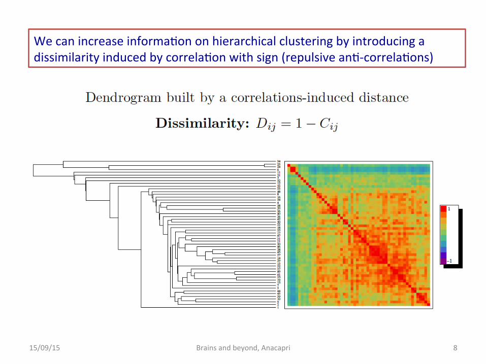
We  can  increase  informa%on  on  hierarchical  clustering  by  introducing  a  dissimilarity  induced  by  correla%on  with  sign  (repulsive  an%-­‐correla%ons)  

15/09/15   Brains  and  beyond,  Anacapri   8  

•  Retaining  the  informa%on  on  the  correla%ons  sign  allows  one  to  clearly  dis%nguish  posi%vely  correlated  groups  of  areas  from  the  nega%vely  correlated  ones,  thus  improving  the  detec%on  of  brain  modules.    

•  Areas  6,  23  and  24  (i.e.  the  lec  part  of  amygdala  and  the  whole  hypothalamus,  respec%vely)  are  recognized  as  forming  a  group  of  highly  posi%vely  correlated  areas,  interac%ng  with  the  rest  of  the  brain  via  quite  large  nega%ve  correla%ons:  this  suggests  that  they  should  be  considered  as  (part  of)  a  separate  module.    

Example  

15/09/15   Brains  and  beyond,  Anacapri   9  

Non-­‐trivial  to  observe  a  hierarchical  structure  in  less  evolved  animals  (e.g.  in  C.  elegans  non  sign  of  hierachical  organiza%on  of  modules)  

Modularity  approach    

Newman  modularity  with  corrected  null  model  for  correla%on  networks  (Louvain’s  detec%on  algorithm)  

[See  M.  MacMahon,  D.  Garlaschelli,  Phys.  Rev.  X  5,  021006  (2015).  M.  E.  J.Newman,  PNAS,  103,  8577  (2006)]  

Only  three  modules  detected  

15/09/15   Brains  and  beyond,  Anacapri   10  

[see  Gallos  et  al.,  PNAS  109,  2825  (2012)  for  “standard”  perc.  under  training  condi%ons]    

Standard  Percola%on  approach  

•  The  abs  values  of  the  measured  correla%ons  are  listed  in  increasing  order;  •  star%ng  from  the  lowest  one,  each  of  them  is  chosen  as  a  threshold;  •  the  links  corresponding  to  the  correla%ons  below  the  threshold  are  removed;  •  the  size  of  the  giant  (largest)  component  is  measured  at  each  step.  

In  Gallos  et  al.  on  human  brain  at  voxel  level  under  strong  external  audio-­‐visual  s%muli    a  step-­‐wise  behavior  is  observed  sugges%ng  a  hierarchical  mul%ple  transi%on  behavior    

Very  different  from  Erdos  Renyi  networks:  STEPS!  

•  We  observe  a  similar  behavior  in  our  case  

•  The  coarse-­‐grained  nature  of  ROI  permits  mul%ple  transi%on  detec%on  also  at  res%ng  condi%on  

15/09/15   Brains  and  beyond,  Anacapri   11  

Our  (varia%on  of  standard)  percola%on  analysis  

•  the  measured  correla%ons  values  r  are  listed  in  increasing  order;  •  star%ng  from  the  lowest  one,  each  of  them  is  chosen  as  a  threshold;  •  the  links  corresponding  to  the  correla%ons  below  the  threshold  are  removed;  •  the  number  of  connected  components  is  computed.  

Step-­‐like  behavior:  at  a  step  the    number  of  connected  components  do  not  increase  by  increasing  r    à The  connected  components  are  “robust”  and  may  indicate  neurophysiological  modules/clusters  (to  be  validated)    Mul)ple  steps  feature  à Hierarchical  organiza=on  of  such  modules/clusters  

BeUer  to  detect  the  hierarchical  organiza%on  of  clusters/modules  In  general  beUer  for  small  networks  where  giant  component  can  be  problema%c  

15/09/15   Brains  and  beyond,  Anacapri   12  

r=0.5   r=0.55  

One  can  check  that  the  use  of  absolute  values  of  Cij  leads  to  spurious  clusters  

15/09/15   Brains  and  beyond,  Anacapri   13  

Minimal  Spanning  Forest  

First  step  of  Kruskal’s  algorithm  for  the  Minimal  Spanning  Tree    

•  Region  pair  (i,j)  are  ordered  in  decreasing  Cij  

•  One  starts  by  drawing  a  graph  from  the  pair  with  the  highest  Cij  

•  One  add  consecu%vely  other  pairs  following  the  order  of  decreasing  Cij  

•  A  pair  is  not  added  to  the  graph  is  the  two  nodes  already  appear  in  the  graph    

In  this  way  a  set  of  disconnected  trees  maximally  correlated  is  obtained    It  correspond  to  the  Minimal  Spanning  Tree  by  removing  the  “weak”  links  connecing  clusters  more  strongly  connected  

15/09/15   Brains  and  beyond,  Anacapri   14  

Typical  MSF  par%%on  in  a  single  mouse  

15/09/15   Brains  and  beyond,  Anacapri   15  

Which  areas  are  the  most  important?  

15/09/15   Brains  and  beyond,  Anacapri   16  

Comparison  with  the  Modularity  analysis  

15/09/15   Brains  and  beyond,  Anacapri   17  

Valida%on  of  results  vs  “randomized”  samples  

Our  real  correla%on  matrices  present  a  quasi-­‐Gaussian  distribu%on  of  entries  

15/09/15   Brains  and  beyond,  Anacapri   18  

Genera%ng  a  “synthe%c”  randomized  brain    

15/09/15   Brains  and  beyond,  Anacapri   19  

15/09/15   Brains  and  beyond,  Anacapri   20  

“Usual”  percola%on  keeps  the  step-­‐wise  feature    

But  it  is  s%ll  step-­‐wise!  

Valida%on  of  percola%on  results  vs  null  model  

15/09/15   Brains  and  beyond,  Anacapri   21  

Sta%s%cal  valida%on  of  the  MSF  

15/09/15   Brains  and  beyond,  Anacapri   22  

Validated  MSF  clusters  

15/09/15   Brains  and  beyond,  Anacapri   23  

What  about  the  “average  mouse”?  

15/09/15   Brains  and  beyond,  Anacapri   24  

Percola%on  on  the  “average  mouse”  

Real  network  

Randomized  

Stepwise  trend:  species-­‐specific  genuine  sign  of  self-­‐organiza%on!  

15/09/15   Brains  and  beyond,  Anacapri   25  

Clusters  of  the  “average  mouse”  

15/09/15   Brains  and  beyond,  Anacapri   26  

15/09/15   Brains  and  beyond,  Anacapri   27  

•  Group  of  areas  previously  iden%fied  with  (part  of)  the  limbic  system  (i.e.  areas  19,  20,  35  and  36  -­‐  the  right  dentate  gyrus  and  the  right  posterior  gyrus)  is  observed  again  and,  further  rising  the  threshold,  the  “core  pairs”  19-­‐35  and  20-­‐36  are  recovered.    

 •  Moreover,  areas  like  the  auditory  (i.e.  7,  8)  and  the  temporal  associa%on  cortex  (i.e.  

49,  50),  are  found  to  be  linked  via  the  double  pair  7-­‐49  and  8-­‐50  (i.e.  the  lec  parts  and  the  right  parts  separately)    

•   network  theory-­‐based  analysis  (percola%on,  modules  detec%on);  

•   defini%on  of  null  models  to  detect  sta%s%cally  significant  signals  of  self-­‐organiza%on  (modular  structure);  

•   correla%ons  are  normally  distributed  at  different  scales;  

•   constraining  the  whole  correla%ons  distribu%on  is  not  enough  to  explain  the  nested  structure  of  real  mice  brains;  

•   the  block-­‐model  \philosophy"  can  be  exported  to  analyse  correla%ons  matrices,  given  the  normal  nested  structure  of  correla%ons  matrices;  

•   much  beUer  results  are  obtained  when  constraining  the  blocks-­‐specific  normal  distribu%ons.  

Conclusions  

15/09/15   Brains  and  beyond,  Anacapri   28  

Villa  (Curzio)  Malaparte:  Masterpiece  of  Adalberto  Libera    15/09/15   Brains  and  beyond,  Anacapri   29  

Thank  you!!