Details for Today:

DATE: 3rd February 2005BY: Mark Cresswell

FOLLOWED BY: Assignment 2 briefing

Evaluation of Model Performance

69EG3137 – Impacts & Models of Climate Change

Lecture Topics• The need to evaluate performance

• Simple spatial correlation

• Bias

• Reliability

• Accuracy

• Skill

• Kolmogorov Smirnov

Why Evaluate?

We must try and objectively and quantitatively assess the performance of any forecasting system

If a climate model performs badly and it is used in critical decision-making processes then poor decisions will be made

End users want an estimate of how confident they can be in predictions made

Climate scientists need to know what models perform best and why

Why Evaluate? #2

A simple deterministic solution has only one outcome – so evaluation is easy (either the event occurred or it did not)

Probabilistic forecasts (giving a percentage chance of an event) requires a method that compares what occurred against the probability weighting that was forecast

Values of model forecast fields may be correlated against reanalysis (observed) fields. This is a preferred method by some climate scientists – but is bad science as discontinuous variables such as rainfall often have skewed distributions

Simple Spatial Correlation

Model grid-points may be matched by corresponding reanalysis grid-points when historical (hindcast) forecasts/simulations are created

The values of each forecast field (temperature, rainfall, humidity, wind velocity etc) may then be compared between model and reanalysis (observed)

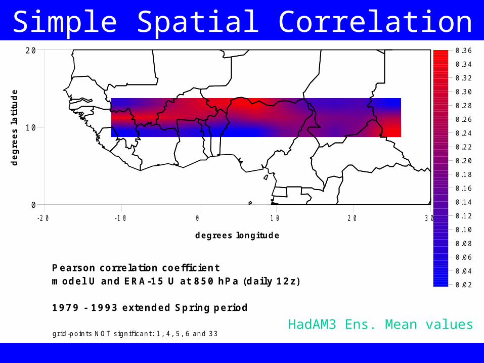
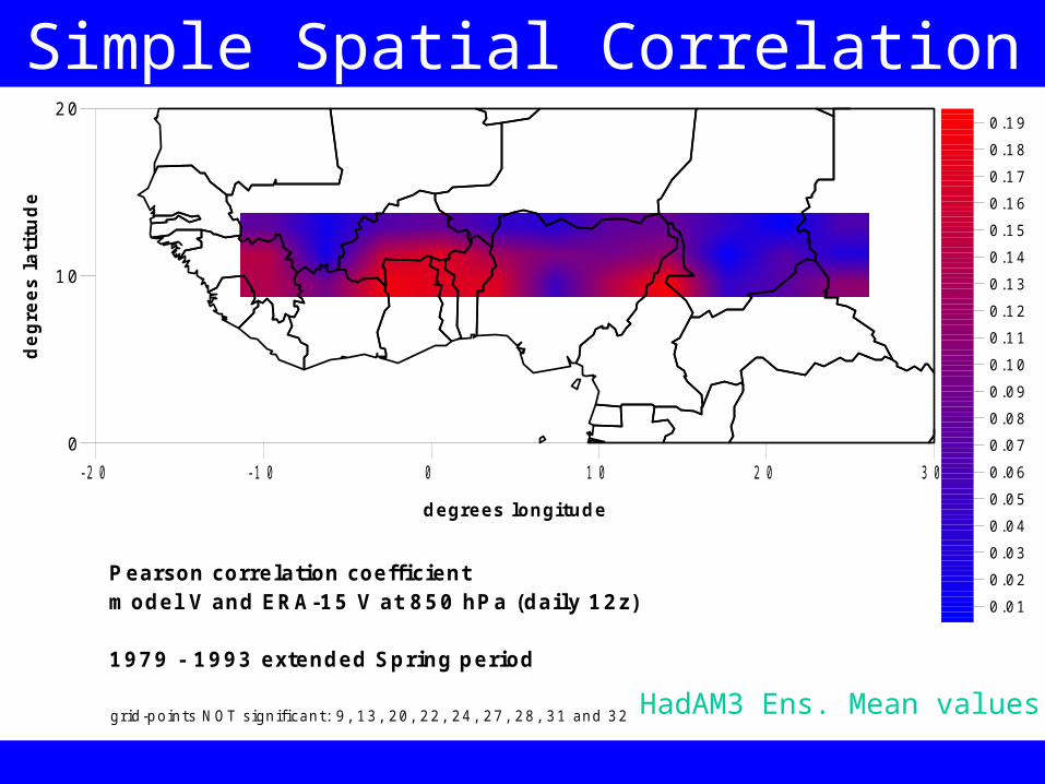
We can quantify the degree of association between forecast and reanalysis fields by performing a simple Pearson correlation test – on a grid-point basis

Simple Spatial Correlation

- 2 0 - 1 0 0 1 0 2 0 3 0

degrees longitude

0

10

20

deg

rees

lat

itu

de

0 .02

0 .04

0 .06

0 .08

0 .10

0 .12

0 .14

0 .16

0 .18

0 .20

0 .22

0 .24

0 .26

0 .28

0 .30

0 .32

0 .34

0 .36

P earson correlation coeffi cientm odel U and ERA-15 U at 850 hP a (daily 12z)

1979 - 1993 extended Spring period

grid -points N OT s ignificant: 1 , 4 , 5 , 6 and 33HadAM3 Ens. Mean values

- 2 0 - 1 0 0 1 0 2 0 3 0

degrees longitude

0

10

20

deg

rees

lat

itu

de

P earson correlation coeffi cientm odel V and ERA-15 V at 850 hP a (daily 12z)

1979 - 1993 extended Spring period

grid -points N OT s ignificant: 9 , 13 , 20 , 22 , 24 , 27 , 28 , 31 and 32

0 .01

0 .02

0 .03

0 .04

0 .05

0 .06

0 .07

0 .08

0 .09

0 .10

0 .11

0 .12

0 .13

0 .14

0 .15

0 .16

0 .17

0 .18

0 .19

Simple Spatial Correlation

HadAM3 Ens. Mean values

Simple Spatial Correlation

-20 -10 0 10 20 30

degrees longitude

0

10

20

degr

ees

latit

ude

0.0 0.1 0.2 0.3 0.4 0.5 0.6

Pearson corre lation (1979 - 1993 data)H adAM 3 U velocity (850 hPa) and X ie-Arkin daily ra in (m m )

Bias

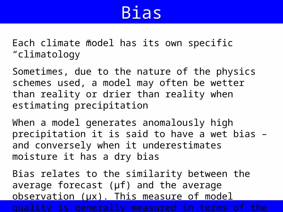
Each climate model has its own specific “climatology”

Sometimes, due to the nature of the physics schemes used, a model may often be wetter than reality or drier than reality when estimating precipitation

When a model generates anomalously high precipitation it is said to have a wet bias – and conversely when it underestimates moisture it has a dry bias

Bias relates to the similarity between the average forecast (µf) and the average observation (µx). This measure of model quality is generally measured in terms of the difference between µf and µx (Katz and Murphy, 1997).

Bias

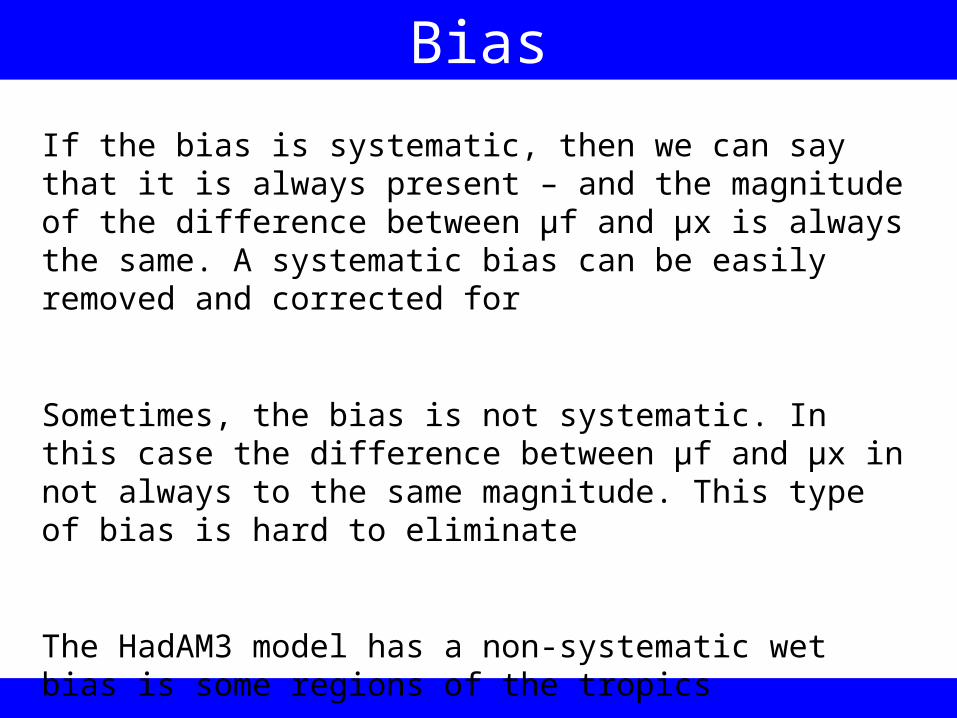
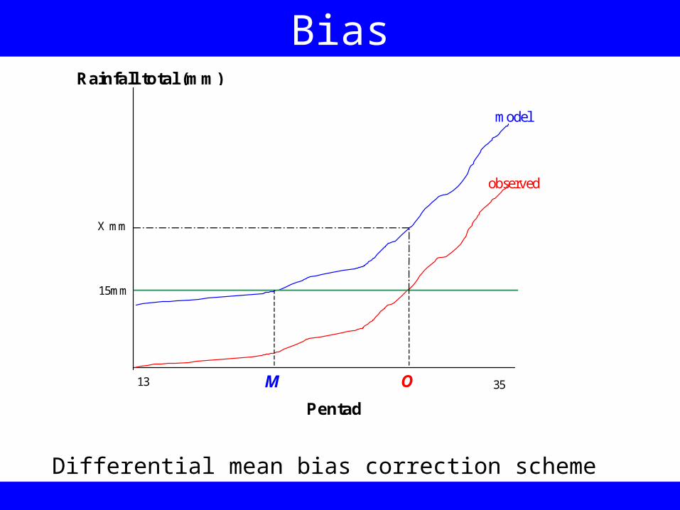
If the bias is systematic, then we can say that it is always present – and the magnitude of the difference between µf and µx is always the same. A systematic bias can be easily removed and corrected for

Sometimes, the bias is not systematic. In this case the difference between µf and µx in not always to the same magnitude. This type of bias is hard to eliminate

The HadAM3 model has a non-systematic wet bias is some regions of the tropics

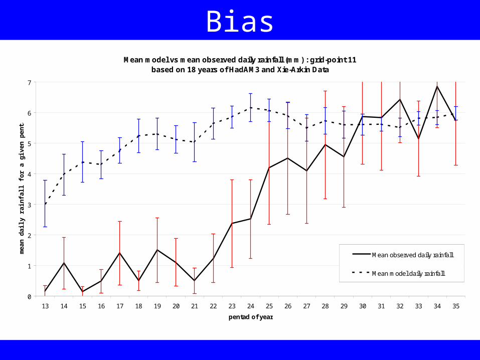
BiasMean model vs mean observed daily rainfall (mm) : grid-point 11

based on 18 years of HadAM3 and Xie-Arkin Data

0

1

2

3

4

5

6

7

13 14 15 16 17 18 19 20 21 22 23 24 25 26 27 28 29 30 31 32 33 34 35

pentad of year

me

an

da

ily

ra

infa

ll f

or

a g

ive

n p

en

tad

(m

m)

Mean observed daily rainfall

Mean model daily rainfall

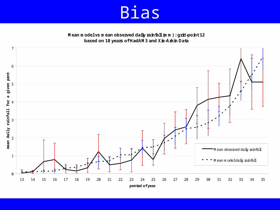
BiasMean model vs mean observed daily rainfall (mm) : grid-point 12

based on 18 years of HadAM3 and Xie-Arkin Data

0

1

2

3

4

5

6

7

13 14 15 16 17 18 19 20 21 22 23 24 25 26 27 28 29 30 31 32 33 34 35

pentad of year

me

an

da

ily

ra

infa

ll f

or

a g

ive

n p

en

tad

(m

m)

Mean observed daily rainfall

Mean model daily rainfall

Bias

Pentad

13 35

15mm

Rainfall total (mm)

OM

X mm

observed

model

Differential mean bias correction scheme

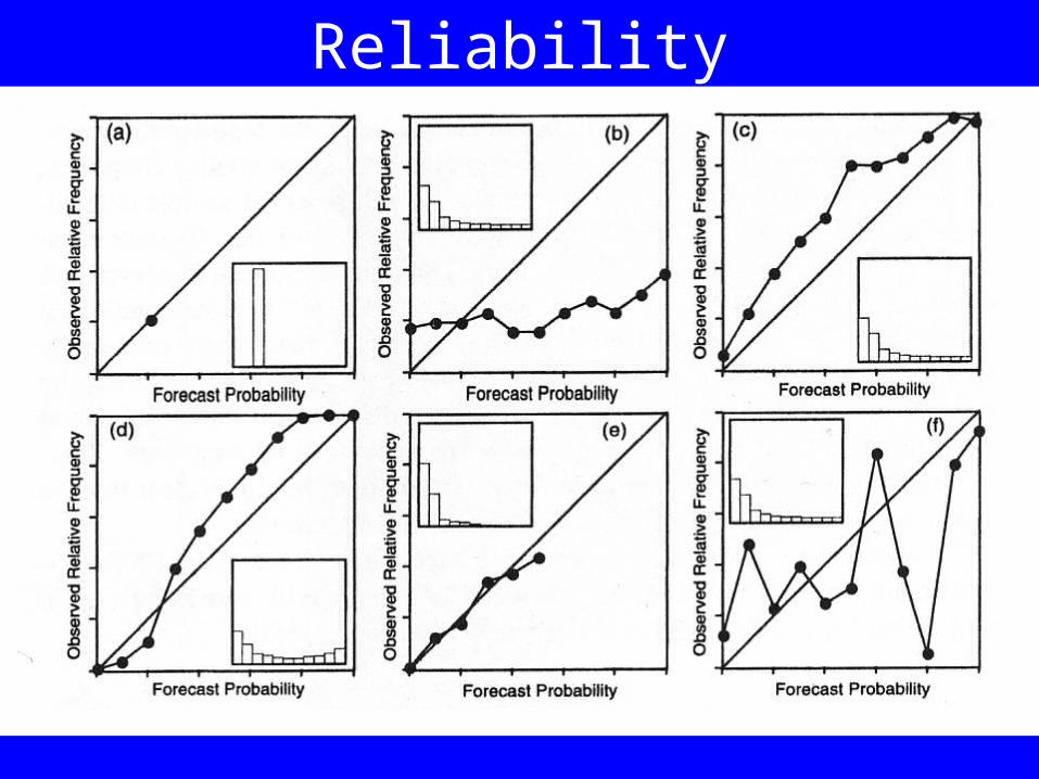
Reliability

Reliability is a measure of association between forecast probability and observed frequency

Suppose a forecast system always gave a probability for above normal rainfall of 80% and below normal of 20%. If after 100 years 80 saw above normal and 20 saw below normal then the model would be 100% reliable.

Notice that reliability is NOT the same as either accuracy or skill

Reliability

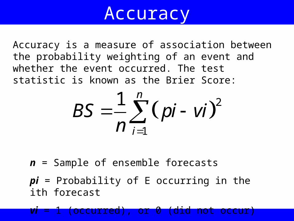
Accuracy

Accuracy is a measure of association between the probability weighting of an event and whether the event occurred. The test statistic is known as the Brier Score:

2

1

1 n

i

BS pi vin

n = Sample of ensemble forecasts

pi = Probability of E occurring in the ith forecast

vi = 1 (occurred), or 0 (did not occur)

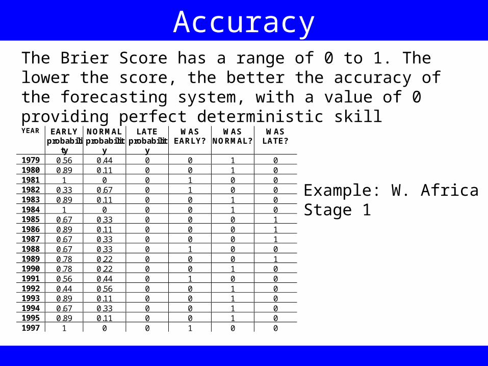
AccuracyThe Brier Score has a range of 0 to 1. The lower the score, the better the accuracy of the forecasting system, with a value of 0 providing perfect deterministic skill

YEAR EARLY probabili

ty

NORMAL probabilit

y

LATE probabilit

y

WAS EARLY?

WAS NORMAL?

WAS LATE?

1979 0.56 0.44 0 0 1 0 1980 0.89 0.11 0 0 1 0 1981 1 0 0 1 0 0 1982 0.33 0.67 0 1 0 0 1983 0.89 0.11 0 0 1 0 1984 1 0 0 0 1 0 1985 0.67 0.33 0 0 0 1 1986 0.89 0.11 0 0 0 1 1987 0.67 0.33 0 0 0 1 1988 0.67 0.33 0 1 0 0 1989 0.78 0.22 0 0 0 1 1990 0.78 0.22 0 0 1 0 1991 0.56 0.44 0 1 0 0 1992 0.44 0.56 0 0 1 0 1993 0.89 0.11 0 0 1 0 1994 0.67 0.33 0 0 1 0 1995 0.89 0.11 0 0 1 0 1997 1 0 0 1 0 0

Example: W. AfricaStage 1

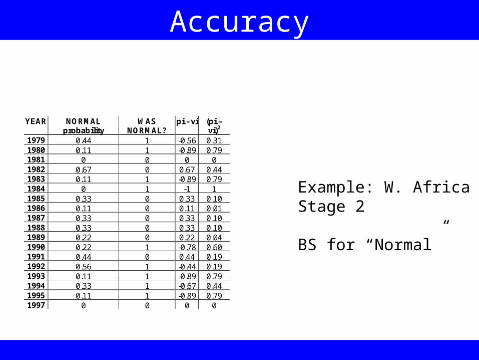
Accuracy

Example: W. AfricaStage 2

BS for “Normal”

YEAR NORMAL probability

WAS NORMAL?

pi - vi (pi – vi)2

1979 0.44 1 -0.56 0.31 1980 0.11 1 -0.89 0.79 1981 0 0 0 0 1982 0.67 0 0.67 0.44 1983 0.11 1 -0.89 0.79 1984 0 1 -1 1 1985 0.33 0 0.33 0.10 1986 0.11 0 0.11 0.01 1987 0.33 0 0.33 0.10 1988 0.33 0 0.33 0.10 1989 0.22 0 0.22 0.04 1990 0.22 1 -0.78 0.60 1991 0.44 0 0.44 0.19 1992 0.56 1 -0.44 0.19 1993 0.11 1 -0.89 0.79 1994 0.33 1 -0.67 0.44 1995 0.11 1 -0.89 0.79 1997 0 0 0 0

Accuracy

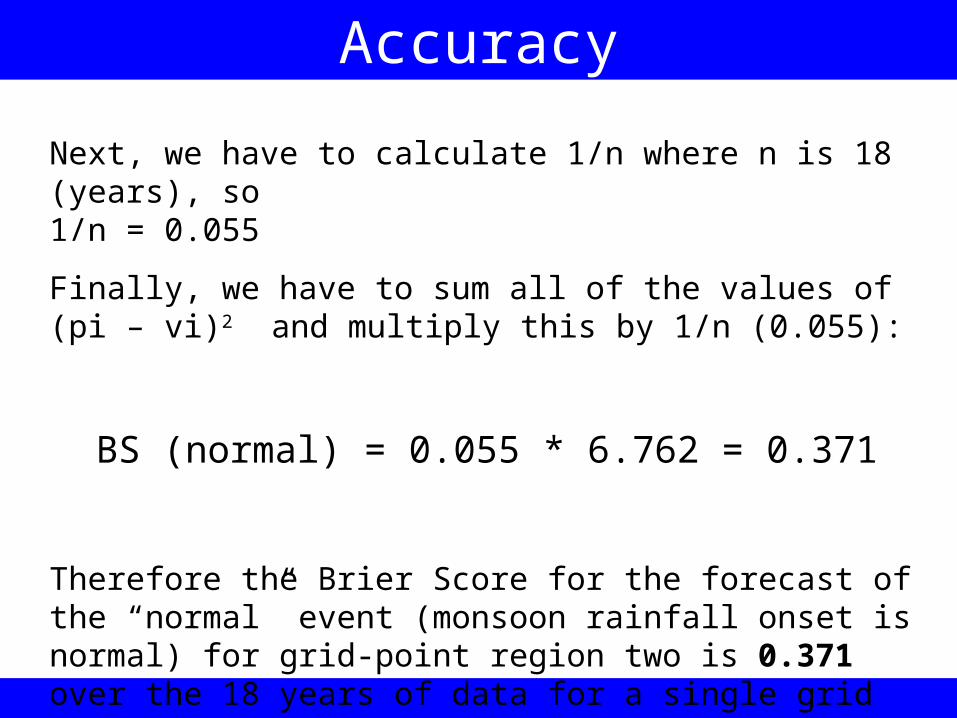
Next, we have to calculate 1/n where n is 18 (years), so 1/n = 0.055

Finally, we have to sum all of the values of (pi – vi)2 and multiply this by 1/n (0.055):

BS (normal) = 0.055 * 6.762 = 0.371

Therefore the Brier Score for the forecast of the “normal” event (monsoon rainfall onset is normal) for grid-point region two is 0.371 over the 18 years of data for a single grid square.

Skill

Skill is a measure of how much more or less accurate our forecast system is compared with climatology. The test statistic is known as the Brier Skill Score:

BSS = Brier Skill Score

Bc = Brier Score (achieved with climatology)

Bf = Brier Score (model simulation)

Bc BfBSS

Bc

Skill

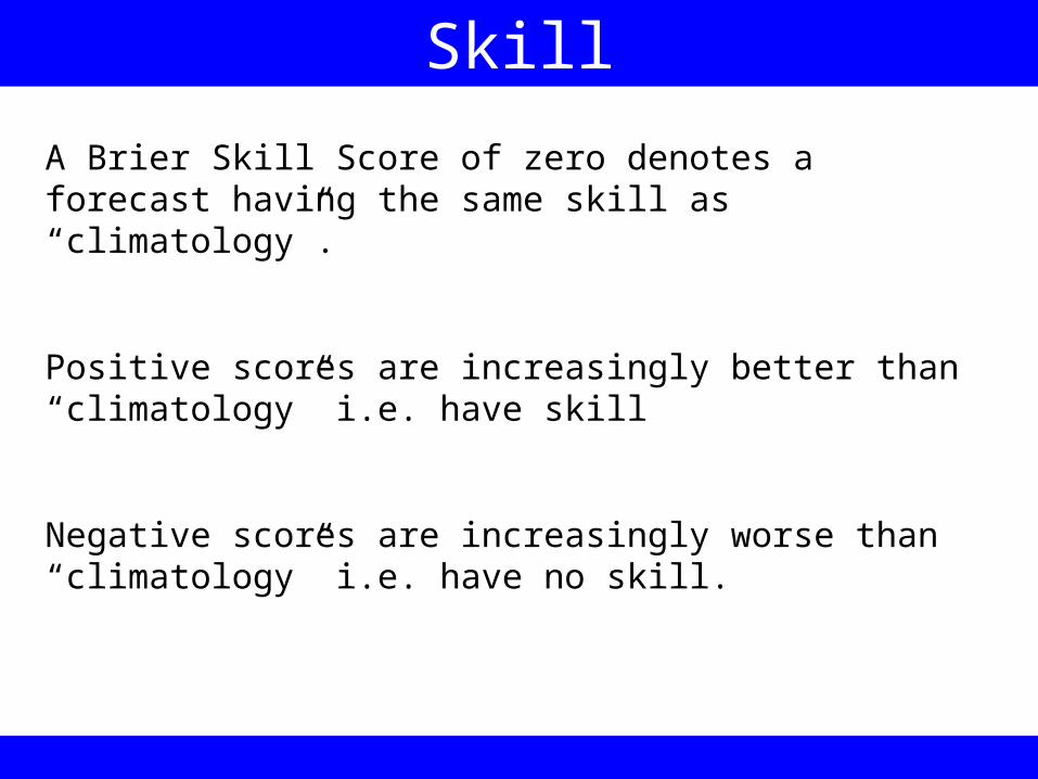
A Brier Skill Score of zero denotes a forecast having the same skill as “climatology”.

Positive scores are increasingly better than “climatology” i.e. have skill

Negative scores are increasingly worse than “climatology” i.e. have no skill.

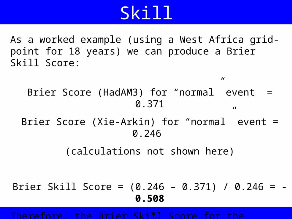
SkillAs a worked example (using a West Africa grid-point for 18 years) we can produce a Brier Skill Score:

Brier Score (HadAM3) for “normal” event = 0.371

Brier Score (Xie-Arkin) for “normal” event = 0.246

(calculations not shown here)

Brier Skill Score = (0.246 – 0.371) / 0.246 = -0.508

Therefore, the Brier Skill Score for the forecast of the “normal” event (monsoon rainfall onset is normal) is -0.508 therefore has no skill.

Kolmogorov Smirnov

The Kolmogorov Smirnov (KS) test tells us how similar two population distributions are

In climate prediction, we might expect our model forecast field distributions to have similar characteristics to climatology – BUT if there is no difference the model is incapable of estimating inter-annual variability

Ideally, we want a model that provides similar, but different, population distributions to climatology.

Kolmogorov Smirnov

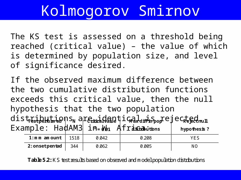
The KS test is assessed on a threshold being reached (critical value) – the value of which is determined by population size, and level of significance desired.

If the observed maximum difference between the two cumulative distribution functions exceeds this critical value, then the null hypothesis that the two population distributions are identical is rejected. Example: HadAM3 in W. Africa:

Test performed N Critical value

= 0.01

Max diff in pop

distributions

Reject null

hypothesis ?

1: mm amount 1518 0.042 0.208 YES

2: onset pentad 344 0.062 0.005 NO

Table 5.2: KS test results based on observed and model population distributions