Detailed Materials and Methods - Nature · first develop allometric relationships between forest biomass and forest timber volume for each forest ... ppt + 1.84×10-5. biomass + 4.42

Detailed Materials and Methods Forest biomass

Forest inventory data are widely used to estimate forest biomass at a national or regional scale. Because they only document information on forest area and forest timber volume, it is necessary to first develop allometric relationships between forest biomass and forest timber volume for each forest type to obtain the biomass expansion factor (BEF, ratio of forest biomass to timber volume)1,2. Previous studies have suggested that the value of BEF varies with forest age, site class, stand density and quality1-3. Nevertheless, timber volume reflects the aggregate effect of changes in all these factors. Hence, BEF can be expressed as an equation of timber volume. We established the relationship for each forest type of China (Supplementary Table S1)1-3. With these BEFs and China’s forest inventory data for the period of 1977-1981, 1984-1988, 1989-1993, 1994-1998, and 1999-20034-8, we estimated forest biomass carbon stock and its change between the 1980s and 1990s for China.

It should be noted that since 1994, the definition of forest in China’s forest inventory has changed from >30% canopy coverage to >20% canopy coverage. This change makes China’s forest inventory comparable with that in other countries because most countries define their forests as above 20% canopy coverage9. As “forest” was defined as larger than 30% canopy coverage in our previous study1, in this study we recalculated forest area, carbon density, and carbon exchange based on the new criterion (20% canopy coverage). However, there was no information on forest area and timber volume with the new criterion in the early inventory data (1977-1981 and 1984-1988). Analyzing the 1994-1998 inventory data which provide both criteria (20% and 30% canopy coverage), we found that there exists a robust linear relationship for the forest area and timber volume between the two criteria at the provincial level (Equations 1 and 2).

AREA0.2 = 1.183AREA0.3 + 12.137 (R2 = 0.990, n=30) (1) TC0.2 = 1.122TC0.3 + 1.157 (R2 = 0.995, n =30) (2)

where AREA0.2 and AREA0.3 are forest areas (104 ha) in a province under the two forest criteria, >20% and >30% canopy coverage, respectively; TC0.2 and TC0.3 are total forest carbon stocks (Tg C; 1 Tg C＝1012 g C＝10-3 Pg C) in a province under the two criteria.

The provincial forest areas and carbon stocks with the new criterion in 1977-1981 and 1984-1988 were calculated based on Equations 1 and 2, and the corresponding forest carbon density were hence obtained. For details, see Fang et al.10. Shrub biomass

Shrub is another widely distributed biome in China with 210×104 km2, about 20% of the country total area. However, studies on carbon cycling in shrublands are very limited. Normalized Difference Vegetation Index (NDVI), defined as the ratio of the difference between near-infrared reflectance and red visible reflectance to their sum, is a good indicator of the fraction of photosynthetically active radiation absorbed by plant canopies11, and thus widely used for biomass estimation12-14. Here, we established a statistical function between NDVI and aboveground biomass to estimate the magnitude and spatial-temporal changes of aboveground biomass for China’s shrub vegetation.

The NDVI data used were from the Global Inventory Monitoring and Modeling Studies (GIMMS) group derived from the National Oceanic and Atmospheric Administration’s Advanced Very High

SUPPLEMENTARY INFORMATIONdoi: 10.1038/nature07944

www.nature.com/nature 1

Resolution Radiometer (NOAA/AVHRR) Land data set, at a spatial resolution of 8×8 km2 and 15-day interval, for the period January 1982 to December 199915,16. The data set has been modified to minimize the effects of volcanic eruptions, solar zenith angle, sensor degradation and other factors, and thus has been carefully optimized17 and been widely used for large-scale studies of ecological processes12, 15, 16, 18, 19. The aboveground biomass data of shrubs, which were used to develop the statistical model, were collected from 34 ecological research sites20-35. The information on shrubland distribution across China was generated from the vegetation map of China with a scale of 1: 4,000,00036.

The growing season average NDVI (NDVIgw) (April to October) was used to develop the statistical model to estimate shrub biomass C density. We calculated the average NDVIgw for the period of 1982-1999, and then obtained mean NDVIgw for each pixel corresponding to the target location by overlying the NDVIgw image over the shrub sites. We therefore developed the statistical model for the relationship between shrub aboveground biomass C density and growing season NDVI, y = 3114.2× NDVI2.3705 (R2=0.28, P<0.01, Figure S1a). Using the model and growing season NDVI from 1982 to 1999, we estimated the magnitude and spatial-temporal changes of shrub aboveground biomass in China between 1982 and 1999.

In shrubland ecosystems, belowground biomass is a key component of the whole ecosystem biomass. Belowground biomass and total biomass were estimated using the ratios of belowground to aboveground biomass obtained from a literature-review (Table S3). We assume that the ratio of belowground to aboveground biomass remains constant for the individual shrub types. Grassland biomass

China has conducted the first national grassland resource survey across more than 2000 counties from 1981 to 198837. This extensive national survey provided mean forage yield data for each grassland type in each province38. Using these data and the method proposed by Fang et al.39, we calculated the aboveground biomass for each grassland type for each province. We use a conversion factor of 0.45 to convert biomass to C content.

In order to estimate the magnitude and spatial-temporal changes of grassland aboveground biomass in China, we developed a statistical function between NDVI and aboveground biomass of grassland in China. Because forage yield reported in DAHV and CISNR38 was measured during the period 1981-1988, we calculated growing season average NDVI for each pixel for the same period to develop the regression relationship between aboveground biomass C density and growing season NDVI (y=291.64×NDVI1.5842, R2=0.72, P<0.001, Figure S1b). We then estimated aboveground biomass C for each pixel for different periods.

Belowground biomass and total biomass were calculated using the ratios of belowground to aboveground biomass for each grassland type40. Similar to shrub, we assume that the ratio of belowground to aboveground biomass remains constant for the same type of grassland. For details, see Piao et al.40. Crop biomass

China is a big agricultural country and agricultural vegetation plays an important role in the carbon cycle. Crop biomass carbon stock can be estimated based on crop yield data and corresponding conversion parameters, as seen in Equation 339.

EPWB /)1( ×−= (3)

where B, W, P, and E are crop biomass, water content of crop economic yield, crop economic yield, and harvest index (the ratio of economic yield to total biomass), respectively. The harvest indices and water contents of crop economic yield are listed in Table S4. A conversion factor of 0.45 was used to convert biomass to carbon content for crops.

Similar to the estimation of shrub biomass carbon stock, using GIMMS NDVI data and agricultural census, we developed a statistical relationship between mean biomass density and NDVI to estimate spatio-temporal change of crop biomass carbon stock (y=1575.2×NDVI2.4201, R2=0.62, P<0.001, Figure S1c).

For the croplands, biomass is subsequently harvested and used, releasing back CO2 to the

doi: 10.1038/nature07944 SUPPLEMENTARY INFORMATION


atmosphere within less than a year41. We thus did not take the biomass increase in standing crop into account in the Chinese C balance. Soil carbon for natural ecosystems

Soils act as sinks or sources for atmospheric CO2, depending mainly on the interactions between ecosystems and climate system. If warming-induced carbon emissions from soil exceed the increase in carbon entering into soil forced by increasing inputs, the soil will be a net carbon source. In order to quantify changes in soil carbon storage over the past two decades, we developed an approach for estimating soil carbon storage of different ecosystems by integrating climate data (temperature and precipitation), NDVI data or biomass data, and ground-based soil inventory data.

In the early 1980s, China conducted the National Soil Survey across the country42-48. The survey resulted in an operational database with 2473 typical soil profiles, which document county name of its geological location, soil depth, organic matter content, soil bulk density, area, annual mean temperature and precipitation, and vegetation types. We use these data to explore carbon stocks of natural soils and their spatial distribution.

In order to detect soil organic carbon changes, first, we calculated SOC density of each soil profile to a depth of 1 m using the following equation:

SOCDh = 0.58 × SOM × BDh × h × (1-Ch/100)/10 (4) where SOCD and SOM are soil organic carbon density (kg m-2) and its content (%), respectively; h (cm) is the thickness of the depth; BDh is bulk density (g cm-3) and Ch (%) is the volume percentage of the fraction > 2 mm at a given depth; and 0.58 is the Bemmelen constant for converting SOM to SOCD.

Second, we classified 2473 typical soil profiles into five categories: evergreen forest soils, deciduous forest soils, shrub soils, grassland soils, and cropland soils. For each soil profile, we calculated the average growing-season NDVI for its corresponding vegetation type at the county where it was sampled. To do so, the county level administrative map and the vegetation map of China with a scale of 1: 4,000,00036 was overlaid with the growing-season NDVI. In addition, for those soil profiles corresponding to forest vegetation cover, we also calculated the forest biomass carbon density at the county where they were sampled by overlying the same vegetation map and county level administrative map with forest biomass carbon density map14.

Third, average growing-season NDVI or biomass carbon density, and annual temperature and precipitation were used to develop a statistical regression to estimate SOC stocks for each vegetation type except for cropland (see next section because of not natural soils) (Equations 5-8). The idea is to model SOC change through calculating change in C input to soil due to changing biomass and change in SOC decomposition induced by climate change over the study period. For the forest category, we used biomass carbon density data as one of the predictors of SOC density in evergreen and deciduous forests instead of NDVI, mainly because biomass could explain more variations of SOC density than NDVI. In addition, due to the human disturbance such as fertilization on cropland soils, SOC of crop was not significantly correlated with NDVI and biomass.

Evergreen forests: Ln(SOCD) = -2.80 × 10-2 temp + 6.05 × 10-5 ppt + 2.20 × 10-4 biomass + 3.77

(R2 = 0.23, P < 0.001) (5) Deciduous forests:

Ln(SOCD) = -7.92 × 10-2 temp + 7.09 × 10-4 ppt + 1.84×10-5 biomass + 4.42 (R2 = 0.29, P < 0.001) (6)

Shrubs: Ln(SOCD) = -4.81 × 10-2 temp + 8.60 × 10-4 ppt + 2.14 NDVI + 2.93

(R2 = 0.33, P < 0.001) (7) Grasslands:

Ln(SOCD) = -0.107 temp + 1.29 × 10-3 ppt + 2.95 NDVI + 3.18 (R2 = 0.53, P < 0.001) (8)

where SOCD is soil organic carbon density (t ha-2) to a depth 1m, temp and ppt are annual mean temperature and precipitation, NDVI denotes average growing season NDVI.



Finally, we calculate the difference between the three-year averaged SOC density for the last period of 1997-1999 and first period of 1982-1984 as the change in SOC density during the 1982-1999 for all grids. SOC density at each grid within each biome can be obtained from the equations forced by annual mean temperature and precipitation data, and the corresponding biomass carbon density (or NDVI) of these two periods. Annual mean temperature and precipitation data at a spatial resolution of 0.1 × 0.1 degrees for the periods of 1982-1999 were derived from the previous studies19, while forest biomass data at a spatial resolution of 0.1 × 0.1 degrees for the periods of 1982-1984 and 1997-1999 were from Piao et al.14. For details, see Wang et al.49. Soil carbon for croplands

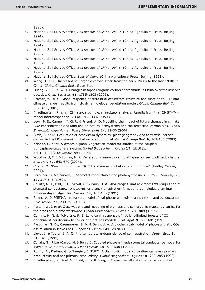
Changes in SOC for China’s croplands over the past two decades were investigated by analyzing the datasets extracted from 132 publications which represented 23 soil groups in terms of FAO/UNESCO taxonomy, with more than sixty thousand soil sample measurements and/or sampling sites (Table S5). The acreage of these soil groups accounts for approximately 76% of the total croplands in mainland China. The results suggest that the soil organic carbon increased by 311–401 TgC (or 0.015-0.020 Pg C yr-1) for China’s croplands over the past 20 years. For details, see ref 50. Ecological process models

Terrestrial ecosystem carbon flux cannot be directly measured at the regional or global scales and thus its estimation by computer models has become an indispensable approach51. During the past decades, several types of models have been developed to estimate terrestrial net ecosystem productivity (NEP) at large scales, but with alternative parameterizations and diverse inclusion of processes51,52. Five process based ecosystem models were applied here: the HyLand model53; the Lund-Potsdam-Jena DGVM54; ORCHIDEE 55; Sheffield –DGVM56 and TRIFFID57.

All models describe surface fluxes of CO2, water (transpiration, photosynthesis, respiration) and the dynamics of water and carbon pools (soil moisture budget, plant C allocation, growth, mortality, soil carbon decomposition) in response to climate change. However, the formulation (and number) of processes primarily responsible for this exchange differ among models. TRIFFID and ORCHIDEE model were originally designed for land surface models in General Circulation Models (GCMs), the other three primarily for offline plant biogeography and land biogeochemistry studies. The major characteristics and differences with respect to carbon exchange are summarized in Table S6. Additional details of how these models represent terrestrial ecosystems have been described elsewhere53-57.

The HyLand model was developed to simulate terrestrial biogeochemical cycles. C3 and C4 photosynthesis in HyLand model are calculated using a biochemical approach based on Farquhar et al.58 and Collatz et al.59, respectively. Stomatal conductance is calculated using empirical relationships between stomatal conductance and irradiance, soil water potential, air temperature, above-canopy water vapour pressure deficit and above-canopy CO2

60. Foliage and fine root maintenance respiration rates are linear functions of N content; sapwood maintenance respiration is a linear function of living sapwood biomass. Herbaceous respiration rates are linear functions of biomass. All respiration components are exponential functions of air temperature. The soil C and N dynamics model is based on Century61 as formulated by Comins and McMurtrie62.

The Lund-Potsdam-Jena DGVM is a process-based biosphere model combining terrestrial vegetation dynamics and biogeochemistry. Plant CO2 assimilation is calculated using the Farquhar photosynthesis model63, as generalized by Collatz et al. 59.Leaf nitrogen and Rubisco activity are assumed to vary both seasonally and with canopy position such as to maximize net assimilation. Maintainance respiration is temperature dependent as described by a modified Arrhenius equation64. Two litter (above and below ground) and two soil pools (fast and slow) are defined. Heterotrophic respiration (Rh) is modeled as a function of litter and soil substrate, tissue-specific base turnover times, temperature, and soil moisture by applying first-order kinetics64, with decomposition of the belowground litter and soil pools dependent on soil temperature, and aboveground litter on air temperature.

ORCHIDEE is a land surface model suitable for coupled simulations within a GCM. Plant CO2



assimilation in the ORCHIDEE model is based on work by Farquhar et al.63 for C3 plants and Collatz et al.65 for C4 plants. Maintenance respiration is a function of each living biomass pool and temperature66. According to the resource balance hypothesis and optimal allocation theory67, plants adjust C allocation among leaves, stem and roots in a way that balances resource acquisition (e.g. carbon, nutrients, and water). ORCHIDEE has eight litter and six soil carbon pools. The evolution of each pool is governed by a first-order linear differential equation, where pool-specific turnovers have soil moisture and soil temperature dependencies. Heterotrophic respiration parameterization is taken from CENTURY68.

The Sheffield –DGVM model is developed to simulate both functional variables (e.g., primary productivity) and structural variables (e.g., leaf area index). Plant CO2 assimilation is based on work by Farquhar et al.63. Stomatal conductance is taken from 69 and Stewart70. Respiration to maintain tissue depends on the mass of living tissue and on temperature. The temperature response function for maintenance respiration was derived from Hay et al.71 and Paembonan et al.72. The soil C and N dynamics model is based on Century61.In addition to the C cycle, Sheffield –DGVM also considers N dynamics.

TRIFFID73 has been developed at the Hadley Centre for use in coupled climate-carbon cycle simulations. Plant CO2 assimilation is coupled to transpiration59, 65. Stomatal conductance and photosynthesis are calculated via a coupled leaf-level model, with leaf area index estimated from a percentage of whole-plant carbon balance. Leaf maintenance respiration is equivalent to the moisture modified canopy dark respiration. Organic matter in the single soil carbon pool decomposes at a rate determined by soil temperature and soil moisture (with maximal decomposition at optimal soil moisture, McGuire et al.74).

Each model was run from its pre-industrial equilibrium at 1901 over the historical period 1901-2002 using observed fields of monthly climatology and annual global atmospheric CO2 concentration75. The meteorological data (air temperature, precipitation, wet day frequency, diurnal temperature range, cloud cover, relative humidity of the air, and wind speed) for 1901-2002 were supplied by the Climatic Research Unit (CRU), School of Environmental Sciences, University of East Anglia, U.K.76, while annual global atmospheric CO2 concentrations for the period 1901-2002 were based on data from ice-core records and atmospheric observations77. It should be noted that none of the models is driven by the satellite derived NDVI data, and thus the results of the model is independent of the approach based on inventory and satellite data. Inverse model

The spatial and temporal characterization of atmospheric CO2 concentration change provides integrated constraints on the net land-atmosphere CO2 exchange78. Inverse models using observed atmospheric CO2 concentration data, atmospheric transport model, and prior information on the land and ocean fluxes have been used to infer spatial patterns of CO2 flux and their interannual variability79-81. This approach is commonly referred to as the “top-down” approach. To our knowledge, there are no reports on the C balance of China’s terrestrial ecosystem derived by inverse models. This may be because 1) most of previous inverse models geographically subdivide the globe into only few continental and ocean regions (e.g. 11 continental regions and 8 ocean regions in the study of Bousquet et al.79) and no individual region’s CO2 flux is predominantly influenced by China’s terrestrial ecosystem and 2) only few stations were available in North Asia. The substantial extension of the monitoring network during the 1990's, together with improved atmospheric models and mathematical methods, however, makes current atmospheric inverse modeling possible to infer with more confidence location, magnitude, and temporal variability of surface sources and sinks of CO2 at relatively high spatial resolutions81.

For this study, new monthly inverse estimates of Net Ecosystem Exchange (NEE) were derived at the spatial resolution of the transport model (LMDz model at 3.75° x 2.5° resolution) for the period 1996-2005. The inverse methodology follows directly from Peylin et al.82. The main components of the system are described below.

Method: We used a Bayesian synthesis inverse method, based on a “matrix” formulation, to solve for monthly fluxes for all grid cells of the transport model. This method allows estimating not



only the magnitude of the fluxes but also their uncertainty (i.e., error variances and covariances). To reduce the size of the inverse problem, we used a sequential approach with consecutive inversions, as in Peylin et al.82. We choose a window of 4 years for each inversion, with a 6 months overlap between the different inversions.

Atmospheric data: We used monthly mean atmospheric CO2 concentrations at 75 stations from the GLOBALVIEW-CO2

84, from the CARBOEUROPE EU-project (for 9 European sites; http://www.carboeurope.org/) and from the NIES Japan laboratory (3 stations over Siberia with aircraft vertical profiles). The location of the stations is given in Figure S2. The spatial coverage favors the Northern hemisphere and especially the European continent. Over North Asia, only 9 stations were available for this study ([TAP, 36°N,126°E], [UUM, 44°N, 111°E], [WLG, 36°N, 100°E], [HAT, 24°N, 123°E], [RYO, 39°N, 141°E], [SUR, 61°N, 73°E], [NOV, 55°N, 83°E], [YAK, 62°N, 130°E], [ZOT, 60°N, 89°E]). The monthly errors were computed as the standard deviation of the CO2 raw data, following the usual assumption that transport models tend to be less reliable for sites with large concentration variability. Typical values range between 0.3 ppm at South Pole station to 5.5 ppm at the Hungarian tall tower station.

Anthropogenic emissions: Fossil fuel CO2 emissions are assumed to be perfectly known, their contribution at each station being pre-subtracted from the CO2 concentration data, to invert the land and ocean fluxes as residuals. The spatial distribution of the fossil fuel emissions follows from Oliver et al.85 and the annual totals are rescaled each year for each country, using the CDIAC statistics. Additionally, we accounted for carbon released to the atmosphere from biomass burning, following the estimates of Van der Werf et al.86. These emissions are used as a prior that is further optimized by the inversion system, for six “large regions” (Europe, North Asia, North America, South America, Africa and South Asia). The spatial and temporal patterns of the emissions are kept fixed to the prior for each region, but the annual carbon fluxes are optimized each year as additional unknowns in the inverse procedure, with an uncertainty of 50%.

Prior land and ocean fluxes: A priori information on the carbon fluxes is taken from ORCHIDEE55 for the terrestrial biosphere and from the climatology of Takahashi et al.87 for the ocean. Note that the ORCHIDEE simulation used for the inversion is different than that used for the ecosystem model comparison discussed above. ORCHIDEE was first run until the carbon pools reach equilibrium (about 1000 years) based on average climate forcing76 from 1980 to 2002 under constant atmospheric CO2 concentration of 350 ppm, and then run using transient climate forcing76 for the period of 1980-2002 without considering atmospheric CO2 increase. The resulting prior land fluxes are thus close to equilibrium and the inversion will locate in space and time a net carbon sink compatible with the atmospheric measurements. Note also that we took the average flux climatology (1996-2002) for the standard inversion and the inter-annual fluxes as a sensitivity test (see below). Prior error on the land is set to 6 Pg C yr-1 globally and spatially distributed according to the Gross Primary Production (GPP) of ORCHIDEE. With this choice tropical regions with large GPP have a larger uncertainty than boreal regions. Spatial flux error correlations are also defined between land grid-points, following an exponential decrease with distance (e-folding length of 1000 km). Temporal error correlations between monthly fluxes are supposed to be negligible. Once the error correlations are defined, we re-scaled the overall error variances-covariances matrix to have a total land a priori flux error of 6 Pg C yr-1. We followed the same approach for ocean fluxes. Prior ocean flux errors are set to 2.5 Pg C yr-1 globally and spatially distributed according to the surface of each ocean grid cell (free of sea-ice). Spatial flux error correlations between ocean grid-points, follow an exponential decrease using an e-folding length of 2000 km.

Transport model: the sensitivities of concentrations at each site and each month to the surface flux of each source region (each model grid-cell during one month), often called influence functions, were calculated with the LMDZ transport model83. LMDZ is a global circulation model that was run with a spatial resolution of 3.75° x 2.5° longitude by latitude with 19 vertical levels. Although the model computes its own dynamics and mass transport, the simulated winds were nudged toward the analyzed fields of ECMWF. We used the retro-transport formulation implemented in LMDZ to efficiently compute the sensitivities of the concentrations to all surface fluxes (one model run for each monthly measurements), as in Peylin et al.82.



In order to test the impact of key components of the inverse system, we realized several inversions, varying successively 1) the number of stations (With only 49 stations excluding new continental sites that are still poorly represented by the model, and without the three Siberian vertical profiles (NOV, SUR, YAK)), 2) the a priori information on land fluxes (using directly the ORCHIDEE NEP simulations instead of the climatology), 3) the prior error on land fluxes (using a smaller total error, 4 PgC yr-1), and 4) the error correlation lengths (using larger error correlations, 2000 km and 3000 km over land and ocean, respectively). Although limited, this set of inversions can be used to estimate potential systematic errors on the regional CO2 fluxes. Since there is a large interannual variability in the terrestrial carbon balance, the mean annual NEE during the period 1996-2005 was used to define current spatial patterns of China’s carbon balance. Finally, note the relatively small number of stations and the difficulties of transport models to represent continental sites still limit the performances of the inversions at regional scale. However, the use of a priori fluxes from the ORCHIDEE land surface model compensates the lack of atmospheric information at the regional scale. The optimized fluxes at small spatial scale should thus be interpreted as a compromise between the information from an ecosystem model and atmospheric CO2 concentrations. Further constraints on the spatial patterns of large scale ecosystem fluxes will be delivered in the future from atmospheric inversions constrained with better datasets.

Three types of uncertainty are estimated for the mean C flux over China. First, a random error associated with the inverse procedure is calculated from the a posteriori flux error covariance matrix, including spatial and temporal error covariances between all grid points within China. Such error depends on the network geometry but also on the choice of a priori flux and data error covariance matrices, so that it remains relatively uncertain. Expressed in terms of error reduction ((posterior – prior) / prior), it reflects the level of constraint brought by the atmospheric network and a comparison between regions informs how well a given region is constrained compared to the others. The error reduction, (posterior – prior)/prior, is 38% for China, a value smaller than for Europe (49%) and North America (56%). Second, we computed a potential systematic error with the standard deviation of the mean fluxes from our ensemble of inversion. This error reflects the impact on the estimated fluxes of critical but uncertain choices for the prior information embedded in the inversion. Finally, we added a third source of errors that specifically correspond to uncertainties in assumed fossil fuel emissions. The uncertainty (20%) of the fossil fuel emissions for whole country was based on the study of Gregg et al.88. We also compared fossil fuel emissions used in this study with that of Ohara et al.89 across the 9 regions (Figure S3). The differences between the two estimates show no systematic spatial pattern so that the inverse derived spatial pattern of NEE might not be significantly affected. These errors estimates are not independent and should be considered as complementary diagnostics.

The mean result of our inversion ensemble is a net CO2 uptake of 0.35 ±0.33 PgC yr-1(with 0.97 Pg C yr-1 of fossil fuel emission), which is comparable to the result of Roedenbeck et al90. They obtained with a different inverse set-up (but still solving for fluxes at the spatial resolution of the transport model) a mean C sink over China of 0.42 Pg C yr-1for the same period, with 0.93 Pg C yr-1 of fossil fuel emissions. If we correct for differences in fossil fuel emissions (0.04 Pg C yr-1 between the two studies), the carbon sink in Roedenbeck et al.90 increases from 0.42 Pg C yr-1 to 0.46 Pg C yr-1, a value that is still compatible with our mean value and error estimates. In addition, our estimation is also comparable with the result of Rayner et al.91 (0.28 Pg C yr-1) and Patra et al.92 (0.40 Pg C yr-1), although both studies may be not appropriated for an estimation of regional carbon fluxes (such as China’s carbon budget), with a system that solves for fluxes over large regions (116 and 66 regions, respectively). In both cases, China extends partially over several of these large regions so that more in-depth analysis of their results would be required for a rigorous comparison with our pixel-based approach. Wood and food trade

We derive import and export data of the forest products from FAO statistical databases93, including roundwood, fuelwood and charcoal, industrial roundwood, sawnwood, wood-based panels, pulp, and paper and paperboard. The data in volume units were transferred to C units using a wood



density of 0.5 and 0.45 carbon concentration in dry biomass94. We calculated 0.008 PgC yr-1 of wood was imported into China.

The import and export data of feed and food products were derived from FAO statistical databases93. The items are listed in food groups as follows: meat and meat preparations, animals and animal fats, dairy products and honey, eggs, beverages, fruits and vegetables, vegetable oils, coffee and tea, cereals, roots and tubers, sugar and sugar crops, oil crops and pulses. FAO statistics give fresh biomass estimates for the above items, and we correct for water content following Goudriann et al.95. With the use of statistical data from FAO93 and approach of Ciais et al.94, we estimated that about 0.004 PgC yr-1 of food was imported into China. Carbon accumulation of the harvested wood products

Carbon accumulated in wood products must be considered in the estimation of regional carbon balance41. In Europe, wood products represent a C sink of about 0.024 PgC yr-1 96. Based on FAO data93, wood products in China are about 43 % of those in Europe. Applying this ratio, we estimated that the C sink of wood products in China was about 0.010 PgC yr-1, which is comparable with the previous estimate of 0.008 PgC yr-1 97. From these two estimates, we took an average estimate of 0.009 PgC yr-1. Export of carbon by Chinese rivers to the ocean

The total annual export of C by Chinese rivers to the ocean has been estimated at between 0.038 and 0.070 PgC yr-1 39, 98-101. We do not know accurately enough which fraction corresponds to CO2 fixed by photosynthesis vs. geological reservoirs; whether this carbon of atmospheric origin has been fixed recently, or is eroded from very old soil pools. Thus, we have not included C leached to rivers in our land-based approaches.



Table S1. Biomass expansion factor (BEF) and its parameters for China’s major forest types. BEF is

calculated by Equation:xbaBEF +＝ , where a and b are constant for a forest type and x is mean

timber volume per hectare. N is number of samples and SD standard deviation.

BEF Parameters Forest type

Mean SD N a b N r2

Abies, Picea 0.89 0.28 36 0.5519 48.861 24 0.78 Cunninghamia lanceolata 0.75 0.18 106 0.4652 19.141 90 0.94

Cypress 1.05 0.29 29 0.8893 7.3965 19 0.87

Larix 0.9 0.22 34 0.6096 33.806 34 0.82

Pinus koraiensis 0.98 0.77 28 0.5723 16.489 22 0.93 P. armandii 0.86 0.19 10 0.5856 18.744 9 0.91 P. massoniana, P. yunnanensis 0.69 0.21 61 0.5034 20.547 52 0.87 P. sylyestris var. mongolica 1.22 0.29 25 1.112 2.6951 15 0.85 P. tabulaefomis 1.00 0.25 127 0.869 9.1212 112 0.91 Other pines and conifer forests 0.89 0.34 39 0.5292 25.087 19 0.86 Tsuga,Cryptomeria,Keteleeria 0.69 0.36 10 0.3491 39.816 30 0.79 Mixed conifer and deciduous 1.31 0.66 11 0.8136 18.466 10 0.99 Betula 1.26 0.27 11 1.0687 10.237 9 0.70 Casuarina 0.93 0.24 11 0.7441 3.2377 10 0.95 Deciduous oaks 1.47 0.35 14 1.1453 8.5473 12 0.98 Eucalyptus 0.9 0.26 20 0.8873 4.5539 20 0.80 Lucidophyllous forests 0.95 0.26 32 0.9292 6.494 24 0.83 Mixed deciduous and Sassafras 1.12 0.36 44 0.9788 5.3764 35 0.93 Nonmerchantable woods 1.31 0.32 20 1.1783 2.5585 17 0.95 Populus 0.9 0.58 29 0.4969 26.973 13 0.92 Tropical forests 0.87 0.22 26 0.7975 0.4204 18 0.87

Table S2. Error estimates of forest growing stock volume and its change for different inventory periods in China. Similar to the approach of Phillips et al.102, we calculate national sampling error (standard error) for growing stock change between preceding and current inventory periods (SE), using China’s forest inventory statistics which provide area, growing stock per unit area (density of growing stock), and number of sampling plots for each forest type for each province. SE is calculated

using mSSRSSSE /)2 212

22

1 ⋅⋅−+= where S12 and S2

2 are national sampling variance of

growing stock for the preceding and current inventory periods; R is the correlation of growing stock between the two inventory periods; and m is number of province-by forest type. CV (coefficient of variance, %) is calculated by 100×SE/mean.

Period Area

(104ha) Growing

stock (104m3)

S (104m3)

Total net change (104m3)

Total SE (104m3)

CV (%)

1984-88 10209 809148 660261 1989-93 10860 908912 585435 99764.1 20570.5 20.62 1994-98 12918 1008585 897442 99672.8 16654.7 16.71 1999-03 14277 1209760 1051403 90562.0 20125.0 22.22 Overall 19.85



Table S3. Ratios of above - to below -ground biomass for 6 shrub types in China.

Shrub type Ratio Reference Sclerophyllus evergreen broadleaf shrubs and dwarf forests on seashore in tropical zone

2.10 (35)

Deciduous shrubs and dwarf forests in temperate and subtropical zones

0.43 (20, 31, 35)

Subalpine deciduous shrubs in temperate and subtropical zones

0.80 (29, 35)

Evergreen and deciduous shrubs and dwarf forests on calcareous soil in subtropical and tropical zones

1.40 (35)

Broadleaf evergreen and deciduous shrubs and dwarf forests on acid soil in subtropical and tropical zones

0.62 (35)

Alpine and subalpine sclerophylla evergreen shrubs and dwarf forests in subtropical zones

1.17 (35)

Table S4. Harvest index and water content of crop economic yield for China’s major crops.

Crop Harvest index Water content Reference

Wheat 0.28-0.46 0.125 (103)

Maize 0.45-0.53 0.13-0.14 (104)

Broomcorn 0.33-0.45 0.14-0.15 (105)

Millet 0.35-0.45 0.125-0.15 (106, 107)

Legume 0.2-0.3 0.12-0.13 (107)

Potato 0.6-0.75 0.133 (107)

Cotton 0.3-0.4 0.083 (107)

Tobacco leaf 0.5 0.082 (107)

Oil plants 0.33-0.45 0.08-0.10 (107)

Hemp 0.33-0.45 0.133 (107)

Sugar crops 0.33-0.45 0.133 (107)

Other crops 0.33-0.45 0.133 (39)



Table S5. Changes of soil organic carbon content in farmland.

Province/City/ Autonomous Region

County or District (City)

Start-End year

Sample no. a)coverage area (×104 ha)

FAO/UNESCO Taxonomy b)

∆SOC (g·kg 1　 ) c)

Reference

Beijing Whole city 1980―1990 1107 34.40 6-1, 8 1.24 (108)

Whole city 1980－2000 (20) na na 1.41 (109) Daxing 1982－2000 267 na 8 2.12 (110) Xuxinzhuang Township 1979－1998 252 0.35 8 2.20 (111) Haidian 1980－2000 104 0.15 na 1.28 (112)

Tianjin Whole city 1980－1991 7119 48.60 na 0.52 (113)

Whole city 1980－1999 (10) na 8 2.95 (114) Jixian 1982－1997 126 1.30 na 1.60 (114)

Hebei Whole province 1982－1996 10310 688.30 na 0.92 (115)

Whole province 1980－2000 (20) na na 2.12 (109) Luancheng 1979－2000 278 3.05 na 3.48 (116) Quzhou 1980－2001 na na 8 2.25 (117) Quzhou 1980－2000 124 na 8 2.38 (118) Daming 1982－1997 108 7.50 8 0.35 (119)

Shanxi Yangcheng 1984－1994 70 3.97 6-1 0.03 (120) Zezhou 1979－1994 221 4.80 6-1 1.57 (121) Inner Mongolia Arong 1982－2002 597 31.25 10, 11-4, 13, 16 12.53 (122) Liaoning Whole province 1979－1999 5551 417.50 6-1, 9, 11-5, 16 0.29 (123)

Kazuo 1981－1997 40(3) 4.36 6-1, 11-5, 16 4.87 (124) Fuxin 1981－1999 224 17.64 6-1, 16 0.91 (125)

Jilin Whole province 1980－2002 (27) 83.19 13 0.41 (126)

Whole province 1980－2000 20 na 13 0.91 (109)

Heilongjiang Whole province 1980－2000 20 360.60 13 7.21 (109)

Whole province 1982－2002 3000 na 13 2.49d)

Shanghai Whole city 1982－2000 (6) 31.50 9 1.78 (127)

Baoshan 1980－1995 73 1.52 na 1.04 (128)

Jiangsu Whole province 1980－2000 80 506.17 9 3.76 (109)

Whole province 1985－1996 (79) na na 2.37 (129) (Wuxi) 1982－1996 na 17.54 9 1.51 (129) (Danyang) 1983－1999 71 5.58 9 2.15 (130)



(Yixing) 1982－1999 105 6.58 9 5.80 (131) (Jintan) 1984－2000 40 4.63 9 3.77 (132) (Nantong) 1982－1997 204 48.32 8, 9, 15 1.22 (133) (Jiangyin) 1981－1996 na 5.18 na 2.60 (134) (Rudong) 1982－1997 1239 11.03 na 1.18 (135) Xincao Farm 1980－2000 181 na 15 0.35 (136) Huaihai Farm 1980－1997 na 0.50 15 2.64 (137) Ganlu Township 1983－2000 77 0.13 9 1.80 (138) (Kunshan) 1981－1997 133 4.70 na 0.99 (139) (Qidong) 1980－1996 50 7.05 8, 15 0.81 (140)

Zhejiang Jiaxing Plain 1982－1995 729 na na 1.51 (141)

(Xiaoshan) 1982－1995 234 5.57 9 1.33 (142) (Cangnan, Chengzhou and Jinhua) 1982－2002 90 23.75 9 0.29 (143)

(Jinhua) 1981－1999 270 18.00 9 0.70 (144) (Jinhua) 1980/81－98/99 715 na na 0.23 (145) Haiyan 1981－2000 na 2.38 na 4.58 (146) (Leqing) 1982－1997 na 11.79 9 4.23 (147) (Cixi) 1981－2002 (6) 2.72 8, 15 1.19 (148) (Shaoxing) 1983－2002 30 16.75 9 0.41 (149) (Ningbo) 1983－99/2000 159 21.64 9 0.93 (150)

Anhui Hanshan 1984－1998 60 4.80 6-19

1.45 4.64

(151)

Lingbi 1984－2002 20

12.07 6-28 9

1.86 0.47 1.68

(152)

Shouxian 1984－2002 192 11.70 9 3.67 (153)

(Liuan) 1984－1998 66 46.60 7

9 2.03 0.93

(154)

Qimen 1984－1999 20 1.33 9 1.59 (155)

Guichi 1984－1999 (5) 2.96 8 9

6.09 8.99

(156)

Changfeng 1981－2003 na 9.00 8 1.10 (157) (Fuyang) 1984－1994 291 133.30 8 0.70 (158) (Chuzhou) 1982－1997 84 40.70 na 1.85 (159)



Qianmiao Township 1982－1998 34 0.35 7, 8, 9 1.45 (160) Fujian (Longyan) 1984－1998 420 13.03 9 3.65 (161)

(Fuan) 1984－1993 1221 2.35 9 4.07 (162) Guangze 1984－2000 na 1.23 9 1.10 (163) (Jianyang) 1984－1998 na 2.85 na 0.70 (164)

Jiangxi Whole province 1981－1997 207 299.34 9 3.54 (165) Nanchang, Xinyu and Xingguo 1981－1997 142

13.90 9 4.64 (166) Nanchang 1981－1997 60 7.21 9, 11-2 5.74 (167) Xingguo 1981－1997 40 3.12 9, 11-2 6.12 (168)

Shandong Huantai 1982－1998 618 3.19 6-1, 6-2, 8 1.14 (169) Henan (Kaifeng) 1984－1998 31 36.30 9 0.65 (170)

(Kaifeng) 1982－1998 62 3.89 1, 8 1.42 (171) Huaxian 1985－2000 300 12.09 8 3.83 (172) (Zhengzhou) 1982－2003 105 9.40 6-1, 8 4.03 (173) (Anyang) 1995－2002 128 36.30 6-1, 8 1.40 (174)

Hubei Sanhu Farm 1981－2000 262 0.38 na 6.11 (175) Hunan Taoyuan 1979－2003 253 4.95 9 4.20 (176)

Taoyuan 1979－2003 85 na 11-2 1.90 (176) Ningxiang 1979－2002 (2) 8.48 9, 11-2 5.77 (177) Xiangyin 1980－2003 (9) 2.35 9 0.46 (178) Twenty counties 1978－1991 300 85.52 na 0.87 (179)

Guangdong Whole province 1980－1990 419 327.22 na 0.41 (180) Baiyun 1980－2002 (12) 0.99 9 0.41 (181)

Guangxi (Guilin) 1979－1998 3536 20.34 9 1.62 (182)

Guanyang 1980－1998 253 1.20 9 4.46 (183) (Binyang, Baise and Liujiang) 1981－2001 107 15.60 na 2.15 (184) Sichuan Pixian 1981－2002 46 2.53 9 1.04 (185)

Yucheng 1981－2002 55 2.35 na 2.25 (186) Five counties 1984－1998 (11) 37.59 2-1, 9, 11-1 1.21 (187) Zitong 1980－2000 (17) 3.36 2-1, 9 1.07 (188) Zizhong 1983－2000 (17) 6.80 na 0.85Jianwei 1981－2000 (17) 7.96 na 1.15 (189)

Guizhou Whole province 1985－2002 310 490.35 914

1.97 1.50

(190)



63% areas of Guizhou Province 1985－1998 149

97.31 9 1.97 (191) 63% areas of Guizhou Province 1985－1998 161 211.61 14 1.51 (192)

Seven counties 1989－1995 (7) 155.02 9 2.04 (192) Xinshi Township 1980－2001 59 0.05 9 8.99 (193)

Shaanxi (Weinan) 1980－1995 157 37.00 3, 4 0.64 (194)

Changwu 1993－2002 59 2.60 4 1.07 (195)

Gansu Whole province 1982－1996 (9) 502.47 2-2, 2-3, 3, 4 1.37 (196)

Gangu 1985－2000 1007 5.98 3, 4 1.10 (197) Qingyang 1982－2000 36 17.00 4 0.17 (198) (Zhangye) 1986－1999 30 8.33 na 2.00 (199)

Qinghai Huzhu 1982－1992/96 160 5.03 2-2, 5, 12 2.39 (200)

Huangshui Watershed 1981－2000/01 81 38.00 2-2, 2-3, 5, 12 2.49 (201) Huangzhong 1986－2001 300 6.07 2-3, 5, 12 4.94 (202)

Ningxia Yinnan Irrigated Prefecture 1984－1993 500 8.91 na 0.05 (203)

Hetao Prefecture 1989－1997 111 0.40 na 0.87 (204) Hetao Prefecture 1989－1998 60 na na 1.44 (205) Yongning 1981－1993 315 3.59 na 0.65 (206)

Xinjiang Bayinguole Municipality 1982－1998 4207 12.85 na 0.57 (207)

Maigaiti 1982－1999 712 2.60 2-3, 8 1.89 (208) Akesu Municipality 1982－2001 na 52.26 2-3, 8, 16 0.87 (209) Hami Municipality 1981－1996 185 4.95 8, 15 0.55 (210) Luntai 1982－1996 416 1.47 2-3, 15, 16 2.20 (211) (Yining) 1981－2001 na 1.58 na 0.81 (212)

a) Numbers in the parenthesis represent the numbers of monitoring sites, counties or soil species. b) 1:Arenosols, 2-1:Calaric regosols, 2-2:Calcaric cambisols, 2-3:Calcaric fluvisols, 3:Calcarus regosols, 4:Calcisols,

5:Chernozems, 6-1:Eutric cambisols, 6-2:Eutric vertisols/gleyic cambisols, 7:Ferric/haplic luvisols, 8:Fluvisols, 9:Fluvisols/cambisols, 10:Gleysols, 11-1:Haplic alisols, 11-2:Haplic alisols/haplic acrisols, 11-3:Haplic calcisols, 11-4:Haplic luvisols/eutric cambisols, 11-5:Haplic/albic luvisols or eutric/dystric cambiosols, 12:Kaslanozems, 13:Phaeozems, 14:Regosols/leptisols, 15:Solonchaks, 16:Umbric gleysols/haplic phacozem

c) ∆SOC is the difference of SOC concentration between the end and the start year. d) Zhang et al., unpublished data.



Table S6. Characteristics of the biogeochemical models75. Process HYLAND LPJ ORCHIDEE (ORC) SDGVM (SHE) TRIFFID (TRI) Photosynthesis Farquhar et al.63 Farquhar et al.63/Collatz et

al.65Farquhar et al.63/Collatz et al.65 Farquhar et al.63/Collatz et

al.65Collatz et al.59/ Collatz et al.65

Stomatal conductance Jarvis69/Stewart70 Haxeltine & Prentice215 Ball et al.218 Leuning220 Cox et al.222

Sapwood respiration f(Assimilation) Gifford213

Dependent on sapwood mass and C:N ratio64

Dependent on temperature, sapwood mass and C:N ratio

Annual sapwood increment, C:N f(T)

Pipe model to diagnose sapwood volume, then Q10 relationship

Fine root respiration f(Assimilation) f(T,Croot) f(T,Croot) f(T,Croot) f(T,Nroot) Evapotranspiration Penman-Monteith

transpiration214Total evapotranspiration216

Transpiration, interception loss, bare ground evaporation and snow sublimation are computed using Monteith-type formulations219

Penman-Monteith transpiration221 + interception + evaporation from soil surface

Penman-Monteith transpiration 221 + interception (Fixed fraction)

Soil water balance 1 soil layer Bucket model

2 soil layers Modified bucket model from Neilson217

2 soil layers (deep bucket layer and upper layer of variable depth)

3 soil + 1 litter layer Modif. Bucket model

4 soil layer Darcy’s law

Litter fall Daily litter carbon balance Annual litter carbon balance

Daily litter carbon balance Monthly litter carbon balance Monthly litter

Hetetrophic respiration CENTURY61 modified by Comins & McMurtrie62

f(T,θtop,tissue type) Based on Parton et al.68 Similar to CENTURY61 f(T,θ,Csoil) McGuire et al.74

C allocation Allometric relationships Annual allometricrelationship for individuals

Based on resource optimization67 Daily allocation by demand in order of priority LAI>roots > wood

Partitioning into ‘spreading’ and ‘growth’ based on LAI leaf:root:wood partitioning from allometric relationships

N uptake f ( soil C, N, T, and moisture)

N allocation Fixed C:N Implicit, dependent on demand

Fixed C:N Variable N with light Fixed C:N



Figure S1. Relationship between aboveground biomass C density (C stock per area) and growing season NDVI of (a) shrub, (b) grassland, and (c) crop in China.

y = 3144.2x2.3705

R2 = 0.2772

0

400

800

1200

1600

0.25 0.3 0.35 0.4 0.45 0.5 0.55

Growing season NDVI

Abo

ve b

iom

ass

dens

ity (g

C/m

2)

(a) Shrub

y = 291.64x1.5842

R2 = 0.72

0

30

60

90

120

150

180

0 0.1 0.2 0.3 0.4 0.5 0.6

Growing season NDVI

Abo

ve b

iom

ass

dens

ity (g

C/m

2)

(b) Grassland

y = 1575.2x2.4201

R2 = 0.6207

0

40

80

120

160

200

0.1 0.15 0.2 0.25 0.3 0.35 0.4

Annual mean NDVI

Abo

ve b

iom

ass

dens

ity (g

C/m

2

(c) Crop

)



Figure S2. Location of the stations used in the inversion.

Fig(20Chi


www.nature.

ure S3. A comparison of average fossil fuel emissions used in this study with that of Ohara et al. 07) across the 9 regions. a: Northeast China; b: Inner Mongolia; c: Northwest China; d: North na; e: Central China; f: Tibetan Plateau; g: Southeast China; h: South China; i: Southwest China.

d

gi

ae

h

cb

f

y = 0.9194xR2 = 0.852

0

100

200

300

0 100 200 300Fossil fuel emissions (Tg C/yr)

(Ohara et al., 2007)

Foss

il fu

el e

mis

sion

s (T

g C

/yr)

(this

stu

dy)

com/nature 17

Supporting References 1. Fang, J. Y., Chen, A. P., Peng, C. H., Zhao, S. Q. & Ci, L. Changes in forest biomass carbon

storage in China between 1949 and 1998. Science 292, 2320-2322 (2001). 2. Fang, J. Y., Oikawa, T., Kato, T., Mo, W. H. & Wang, Z. H. Biomass carbon accumulation by

Japan’s forests from 1947 to 1995. Global Biogeochem. Cycles 19, GB2004, doi:10.1029/2004GB002253 (2005).

3. Fang, J. Y., Wang, G. G., Liu, G. H. & Xu, S. L. Forest biomass of China: An estimate based on the biomass-volume relationship. Ecol. Appl. 8, 1084-1091 (1998).

4. Chinese Ministry of Forestry, Forest Resource Statistics of China for Period 1977-81 (Department of Forest Resource and Management, Chinese Ministory of Forestry, Beijing, 1982).

5. Chinese Ministry of Forestry, Forest Resource Statistics of China for Period 1984-88 (Department of Forest Resource and Management, Chinese Ministory of Forestry, Beijing, 1989).

6. Chinese Ministry of Forestry, Forest Resource Statistics of China for Periods and 1989-1993 (Department of Forest Resource and Management, Chinese Ministory of Forestry, Beijing, 1994).

7. Chinese Ministry of Forestry, Forest Resource Statistics of China for Periods 1994-98 (Department of Forest Resource and Management, Chinese Ministory of Forestry, Beijing, 1999).

8. Chinese Ministry of Forestry, Forest Resource Statistics of China for Periods 1999-2002 (Department of Forest Resource and Management, Chinese Ministory of Forestry, Beijing, 2004).

9. UNECE/FAO (United Nations Economic Commission for Europe/Food and Agriculture Organization of the United Nations), Forest resources of Europe, CIS, North America, Japan, New Zealand: UNECE/FAO contribution to the global forest resources assessment 2000 (United Nations, Geneva, 2000).

10. Fang, J. Y., Guo, Z. D., Piao, S. L. & Chen, A. P. Terrestrial vegetation carbon sinks in China, 1981-2000. Sci. in China Ser. D-Earth Sci. 50, 1341-1350 (2007).

11. Tucker, C. J., Fung, I. Y., Keeling, C. D. & Gammon, R. H. Relationship between atmospheric CO2 variations and a satellite-derived vegetation index. Nature 319, 195-199 (1986).

12. Myneni, R. B. et al. A large carbon sink in the woody biomass of Northern forests. Proc. Natl. Acad. Sci. U.S.A. 98, 14784-14789 (2001).

13. Dong, J. R. et al. Remote sensing estimates of boreal and temperate forest woody biomass : carbon pools, sources, and sinks. Remote Sens. Environ. 84, 393-410 (2003).

14. Piao, S. L., Fang, J. Y., Zhu, B. & Tan, K. Forest biomass carbon stocks in China over the past two decades: Estimation based on integrated inventory and satellite data. J. Geophys. Res.-Biogeosci. 110, G01006, doi:10.1029/2005JG000014 (2005).

15. Tucker, C. J. et al. Higher northern latitude normalized difference vegetation index and growing season trends from 1982 to 1999. Int. J. Biometeor. 45, 184-190 (2001).

16. Zhou, L. M. et al. Variations in northern vegetation activity inferred from satellite data of vegetation index during 1981 to 1999. J. Geophys. Res.-Atmos. 106, 20069-20083 (2001).

17. Slayback, D. A., Pinzon, J. E., Los, S. O. & Tucker, C. J. Northern hemisphere photosynthetic trends 1982-99. Global Change Biol. 9, 1-15 (2003).

18. Fang, J. Y., Piao, S. L., He, J. S. & Ma, W. H. Increasing terrestrial vegetation activity in China, 1982-1999. Sci. in China Ser. C-Life Sci. 47, 229-240 (2004).

19. Piao, S. L. et al. Interannual variations of monthly and seasonal normalized difference vegetation index (NDVI) in China from 1982 to 1999. J. Geophys. Res.-Atmos. 108, 4401, doi:10.1029/2002JD002848 (2003).

20. Shangguan, T. L. & Zhang, F. On synecological features and biomass of Ostryopsis davidiana Yunding mountain, Shanxi province. J. Shanxi Univ. (Nat. Sci. Ed.) 12, 347-352 (1989).

21. Jin, X. H., Song, Y. C. & Zuo, W. J. A study on the biomass of secondary shrub thicket and



shrub-grassland in Yi country of Anhui province. Acta Ecol. Sin. 10, 328-332 (1990). 22. Ding, S. Y. & Peng, J. A study on biomass of Castanopsis Orthacantha sprouted shrub

community in Kunming region. J. Southwest For. Coll. 11, 41-50 (1991). 23. Ou, X. K. & Zhang, Y. C. Primary study on the population pattern of dominant species and

biomass of Quercus langispica sprouted shrub community. J. Yunan Univ. (Nat. Sci.) 14, 198-201 (1992).

24. Peng, J., Su, W. H., Wang, B. R. & Ding, S. Y. Studies on the biomass and net primary production of Lithocarpus Dealbatus sprouted shrub community. J. Yunan Univ. (Nat. Sci.) 14, 179-184 (1992).

25. Su, W. H., Peng, J., Wang, B. R. & Ding, S. Y. Studies on the aboveground biomass and the net primary of Quercus Longispica sprouted shrub community. J. Yunan Univ. (Nat. Sci.) 14, 185-190 (1992).

26. Liao, B. W., Zheng, D. Z. & Zheng, S. F. Studies of the biomass of Sonneratia, Caseolaris stand. For. Res. 6, 680-685 (1993).

27. Zhu, X. W., Shi, Q. M. & Li, Y. L. A preliminary study of the biomass of arbor-shrub in Datong, Qinghai. Qinghai Agric. For. Sci. Technol. 1, 15-20 (1993).

28. Heimann, M. et al. Evaluation of terrestrial Carbon Cycle models through simulations of the seasonal cycle of atmospheric CO2: First results of a model intercomparison study. Global Biogeochem. Cycles 12, 1-24 (1998).

29. Yu, Y. W., Hu, Z. Z., Zhang, D. G. & Xu, C. L. The net primary productivity of Potentilla fcuticosa shrub. Acta Pratac. Sin. 9, 33-39 (2000).

30. Zhang, G. F. & Song, Y. C. Studies on the Biomass of Castanopsis sclerophylla+Quercus Fabri Shrubland in Tiantong Region，Zhejiang Province. J. Wuhan Botan. Res. 19, 101-106 (2001).

31. Chen, X. L. et al. Studies of the biomass and productivity of typical shrubs in Taiyue Mountain, Shanxi Province. For. Res. 15, 304-309 (2002).

32. Zhou, H. K. et al. Study of formation pattern of below-ground biomass in Potentilla fruticosa shrub. Acta Pratac. Sin. 11, 59-65 (2002).

33. Liu, G. H. et al. Aboveground biomass of main shrubs in dry valley of Minjiang River. Acta Ecol. Sin. 23, 1757-176 (2003).

34. Liu, J. H., Xu, X. X., Yang, G., Mu, X. M. & Wang, W. Study on biomass of secondary shrubbery community in small watershed of Loess Hill and Gully Region. Acta Bot. Boreali-occidentalia Sin. 23, 1362-1366 (2003).

35. Hu, H. F., Wang, Z. H., Liu, G. H. & Fu, B. J. Vegetation carbon storage of major shrublands in China. J. Plant Ecol. 30, 539-544 (2006).

36. IGCAS (Institute of Geography, Chinese Academy of Sciences), Digitized Vegetation Map of China (National Laboratory for GIS and Remote Sensing, Beijing, 1996).

37. DAHV (Department of Animal Husbandry and Veterinary, Institute of Grassland, Chinese Academy of Agricultural Sciences) and GSAHV (General Station of Animal Husbandry and Veterinary, China Ministry of Agriculture), Rangeland Resources of China (China Agricultural Science and Technology Press, Beijing, 1996).

38. DAHV (Department of Animal Husbandry and Veterinary, Institute of Grassland, Chinese Academy of Agricultural Sciences) and CISNR (Commission for Integrated Survey of Natural Resources, Chinese Academy of Sciences), Data on Grassland Resources of China (China Agricultural Science and Technology Press, Beijing, 1994).

39. Fang, J. Y., Liu, G. H. & Xu, S. L. in Emissions and their relevant processes of greenhouse gases in China (eds Wang, G. C. & Wen,Y. P.) 81-149 (Chinese Environmental Science Publishers, Beijing, 1996).

40. Piao, S. L., Fang, J. Y., Zhou, L. M., Tan, K. & Tao, S. Changes in biomass carbon stocks in China's grasslands between 1982 and 1999. Global Biogeochem. Cycles 21, GB2002, doi:10.1029/2005GB002634 (2007).

41. Pacala, S. W. et al. Consistent land- and atmosphere-based US carbon sink estimates. Science 292, 2316-2320 (2001).

42. National Soil Survey Office, Soil species of China, Vol. 1.(China Agricultural Press, Beijing,



1993). 43. National Soil Survey Office, Soil species of China, Vol. 2. (China Agricultural Press, Beijing,





1996). 48. National Soil Survey Office, Soils of China (China Agricultural Press, Beijing, 1998). 49. Wang, T. et al. Increased soil organic carbon stock from the early 1980s to the late 1990s in

China. Global Change Biol., Submitted. 50. Huang, Y. & Sun, W. J. Changes in topsoil organic carbon of croplands in China over the last two

decades. Chin. Sci. Bull. 51, 1785-1803 (2006). 51. Cramer, W. et al. Global response of terrestrial ecosystem structure and function to CO2 and

climate change: results from six dynamic global vegetation models.Global Change Biol. 7, 357-373 (2001).

52. Friedlingstein, P. et al. Climate-carbon cycle feedback analysis: Results from the (CMIP)-M-4 model intercomparison. J. Clim. 19, 3337-3353 (2006).

53. Levy, P. E., Cannell, M. G. R. & Friend, A. D. Modelling the impact of future changes in climate, CO2 concentration and land use on natural ecosystems and the terrestrial carbon sink. Global Environ.Change-Human Policy Dimensions 14, 21-30 (2004).

54. Sitch, S. et al. Evaluation of ecosystem dynamics, plant geography and terrestrial carbon cycling in the LPJ dynamic global vegetation model. Global Change Biol. 9, 161-185 (2003).

55. Krinner, G. et al. A dynamic global vegetation model for studies of the coupled atmosphere-biosphere system. Global Biogeochem. Cycles 19, GB1015, doi:10.1029/2003GB002199 (2005).

56. Woodward, F. I. & Lomas, M. R. Vegetation dynamics - simulating responses to climatic change. Biol. Rev. 79, 643-670 (2004).

57. Cox, P. M. “Description of the "TRIFFID" dynamic global vegetation model” (Hadley Centre, 2001).

58. Farquhar, G. & Sharkey, T. Stomatal conductance and photosynthesis. Ann. Rev. Plant Physiol. 33, 317-345 (1982).

59. Collatz, G. J., Ball, J. T., Grivet, C. & Berry, J. A. Physiological and environmental-regulation of stomatal conductance, photosynthesis and transpiration-A model that includes a laminar boundarylayer. Agri. For. Meteor. 54, 107-136 (1991).

60. Friend, A. D. PGEN-An integrated model of leaf photosynthesis, transpiration, and conductance. Ecol. Model. 77, 233-255 (1995).

61. Parton, W. J. et al. Observations and modeling of biomass and soil organic-matter dynamics for the grassland biome worldwide. Global Biogeochem. Cycles 7, 785-809 (1993).

62. Comins, H. N. & McMurtrie, R. E. Long-term response of nutrient-limited forests of CO2 enrichment-equilibrium behavior of plant-soil models. Ecol. Appl. 3, 666-681 (1993).

63. Farquhar, G. D., Caemmerer, S. V. & Berry, J. A. A biochemical-model of photosynthetic CO2 assimilation in leaves of C-3 species. Planta 149, 78-90 (1980).

64. Lloyd, J. & Taylor, J. A. On the temperature-dependence of soil respiration. Funct. Ecol. 8, 315-323 (1994).

65. Collatz, G., Ribas-Carbo, M. & Berry, J. Coupled photosynthesis stomatal conductance model for leaves of C4 plants. Aust. J. Plant Physiol. 19, 519-538 (1992).

66. Ruimy, A., Dedieu, G. & Saugier, B. TURC: A diagnostic model of continental gross primary productivity and net primary productivity. Global Biogeochem. Cycles 10, 269-285 (1996).

67. Friedlingstein, P., Joel, G., Field, C. B. & Fung, I. Toward an allocation scheme for global



terrestrial carbon models. Global Change Biol. 5, 755-770 (1998). 68. Parton, W., Stewart, J. & Cole, C. Dynamics of C, N, P, and S in grassland soil: A model.

Biogeochemistry 5, 109-131 (1988). 69. Jarvis, P. G. Interpretation of variations in leaf water potential and stomatal conductance found

in canopies in field. Phil. Trans. Series B-Biological Sci. 273, 593-610 (1976). 70. Stewart, C. A. Impact of ozone on the reproductive biology of Brassica campestris L. and

Plantago major L. PhD thesis (University of Loughborough, UK, 1998). 71. Hay, R. K. M. & Delecolle, R. The setting of rates of development of wheat plants at crop

emergence-influence of the environment on rates of leaf appearance. Ann. Appl. Biol. 115, 333-341 (1989).

72. Paembonan, S. A., Hagihara, A. & Hozumi, K. Long-term measurement of CO2 release from aboveground parts of a hinoki forest tree in relation to air temperature. Tree Physiol. 8, 399-405 (1991).

73. Cox, P. M. Description of the TRIFFID dynamic global vegetation model (Hadley Centre Tech. Note 24, Met Office, Bracknell, United Kingdom, 2001) [Available online at www.metoffice.gov.uk/research/hadleycentre/pubs/HCTN/HCTNp24.pdf].

74. McGuire, A. D. et al. Interactions between carbon and nitrogen dynamics in estimating net primary productivity for potential vegetation in North America. Global Biogeochem. Cycles 6, 101-124 (1992).

75. Sitch, S. et al. Evaluation of the terrestrial carbon cycle, future plant geography and climate carbon cycle feedbacks using 5 Dynamic Global Vegetation Models (DGVMs). Global Change Biol. 14, 1-25 (2008).

76. Mitchell, T. D. & Jones, P. D. An improved method of constructing a database of monthly climate observations and associated high-resolution grids. Int. J. Climatol. 25, 693-712 (2005).

77. Keeling, C. D. & Whorf, T. P. in A compendium of data on global change (ed. O. R. N. L. Carbon Dioxide Information Analysis Center, U.S.) (Oak Ridge, Tenn, 2005).

78. Keeling, C. D., Whorf, T. P., Wahlen, M. & Vanderplicht, J. Interannual extremes in the rate of rise of atmospheric carbon dioxide since 1980. Nature 375, 666-670 (1995).

79. Bousquet, P. et al. Regional changes in carbon dioxide fluxes of land and oceans since 1980. Science 290, 1342-1346 (2000).

80. Gurney, K. R. et al. Towards robust regional estimates of CO2 sources and sinks using atmospheric transport models. Nature 415, 626-630 (2002).

81. Baker, D. F. et al. TransCom 3 inversion intercomparison: Impact of transport model errors on the interannual variability of regional CO2 fluxes, 1988-2003. Global Biogeochem. Cycles 20, GB1002, 10.1029/2004GB002439 (2006).

82. Peylin, P. et al. Daily CO2 flux estimates over Europe from continuous atmospheric measurements: 1, inverse methodology. Atmos. Chem. Phys. 5, 3173-3186 (2005).

83. Hourdin, F & Armengaud, A. The use of finite-volume methods for atmospheric advection of trace species. Part I: Test of various formulations in a general circulation model. Mon. Weather Rev., 127, 822-837 (1999)

84. GLOBALVIEW-CO2. Cooperative Atmospheric Data Integration Project Carbon Dioxide. CD-ROM, NOAA CMDL (Also available on Internet via anonymous FTP to ftp.cmdl.noaa.gov, Path: ccg/co2/GLOBALVIEW) (2007).

85. Olivier, J. G. J. & Berdowski, J. J. M. Global emissions sources and sinks, in The Climate System, Berdowski, J., Guicherit, R. & Heij, B. J. Eds., (Balkema, A.A. Publishers/Swets & Zeitlinger Publishers, Lisse, The Netherlands, 2001).

86. van der Werf, G.R. et al. Interannual variability in global biomass buring emissions from 1997 to 2004. Atmos. Chem. Phys. 6, 3423-3441 (2006).

87. Takahashi, T. et al. Global air-sea flux of CO2: An estimate based on measurements of sea-air pCO2 difference. Proc. Nat. Acad. Sci. U.S.A. 94, 8292-8299 (1997).

88. Gregg, J., Andres, S. & Marland, G. China: Emissions pattern of the world leader in CO2 emissions from fossil fuel consumption and cement production. Geophys. Res. Lett. 35, L08806, doi:10.1029/2007GL032887 (2008).



http://www.metoffice.gov.uk/research/hadleycentre/pubs/HCTN/HCTNp24.pdf

89. Ohara, T. et al. An Asian emission inventory of anthropogenic emission sources for the period 1980-2020. Atmos. Chem. Phys. 7, 4419-4444 (2007).

90. Rodenbeck, C. & Heimann, M. Jena CO2 Inversion. [http://www.bgc-jena.mpg.de/~christian.roedenbeck/download_CO2/].

91. Rayner, P.J. et al. Two decades of terrestiral carbon fluxes from a carbon cycle data assimilation system. Global Biogeochem. Cycles 19, GB2026, doi:10.1029/2004GB002254 (2005).

92. Patra, P.K. et al. Interannual and decadal changes in the sea-air CO2 flux from atmospheric CO2 inverse modeling. Global Biogeochem. Cycles 19, GB4013, doi:10.1029/2004GB002257 (2005).

93. FAO Statistical databases. http://www.fao.org/waicent/portal/statistics_en.asp. 94. Ciais, P. et al. The impact of lateral carbon fluxes on the European carbon balance. Biogeosci.

Discuss 3, 1529-1559 (2006). 95. Goudriaan, J., Groot, J. J. R. & Uithol, P. W. J. in Terrestrial Global Productivity (eds Roy, J.,

Saugier, B. & Mooney, H. A.) 35 (Academic Press, San Diego, 2001). 96. Janssens, I. A. et al. Europe's terrestrial biosphere absorbs 7 to 12% of European anthropogenic

CO2 emissions. Science 300, 1538-1542 (2003). 97. Kohlmaier, G., Kohlmaier, L., Fries, E. & Jaeschke, W. Application of the stock change and the

production approach to Harvested Wood Products in the EU-15 countries: a comparative analysis. Eur. J. For. Res. 126, 209-223 (2007).

98. Ludwig, W., Probst, J. & Kempe, S. Predicting the oceanic input of organic carbon by continental erosion. Global Biogeochem. Cycles 10, 23-41 (1996).

99. Zhang, S., Gan, W. B. & Ittekkot, V. Organic-matter in large turbid rivers - the Huanghe and its estuary. Mari. Chem. 38, 53-68 (1992).

100. Gao, Q. Z., Shen, C. D., Sun, Y. M. & Yi, W. X. The organic carbon weathering fluxes in Xijiang river basinage. Acta Sediment. Sin. 18, 639-645 (2000).

101. Gao, Q. Z., Shen, C. D., Sun, Y. M. & Yi, W. X. A preliminary study on the organic carbon weathering fluxes in Beijiang river basinage. Environ. Sci. 22, 12-18 (2001).

102. Phillips, D. L., Brown, S. L., Schroeder P. E. & Birdsey, R. A. Toward error analysis of large-scale forest carbon budgets. Global Ecol. Biogeo. 9, 303-313 (2000).

103. Huang, X. H. Cultivate Physiology of Wheat (Shanghai Science and Technology Press, Shanghai, 1984).

104. Shangdong Academy of Agricultural Sciences, Chinese Corn Planting (Shanghai Science and Technology Press, Shanghai, 1986).

105. Liaoning Academy of Agricultural Sciences, Chinese Broomcorn Planting (Agriculture Press, Beijing, 1988).

106. Shanxi Academy of Agricultural Sciences, Chinese Millets Planting (Agriculture Press, Beijing, 1987).

107. Editorial Committee for Chinese Agriculture Encyclopedia, Encyclopedia of Chinese Agriculture, Field Crop Volumn (Agriculture Press, Beijing, 1991).

108. Zhang, Y. S. Study on the improvement of farmland nutrients and advised fertilizer recommendation in Beijing. Chin. J. Soil Sci. 27, 107110 (1996).

109. Yu, H., Huang, J. K. & Scott, R. Soil fertility changes of cultivated land in eastern China. Geogr. Res. 22, 380-388 (2003).

110. Wang, R., Zhang, F. R. & Wang, J. Y. Temporal changing of plant nutrients in different texture soils in the plain of northern China. Chin. J. Soil Sci. 32, 255257 (2001).

111. Yao, J. Changes in farmland fertility at town level and advised on fertilizer recommendation. Beijing Agric. Sci. 18, 25-29 (2000).

112. Su, L. X., Xiao, J. & Wang, S. Q. Status and change of arable soil nutrients in Haidian District of Beijing. Soil Fert. 5, 17-20 (2004).

113. Regional Planning Office of Agriculture Commission in Tianjing, Analysis of Soil Nutrients Variation Trend in Tianjing (Journal of China Agricultural Resources and Regional Planning, ed.3, 1994) 60-64.

114. Chen, Z. X., Li, Y. F. & Liu, Z. J. The primary oriented monitoring report of soil fertility in Tianjin.



Tianjin Agro-For. Technol. 3, 1-3 (2001). 115. Guo, J., Xing, Z. & Li, C. J. Study on the effects of fertilizer and straw return to soil on plow land

nutrients variety. J. Hebei Agric. Sci. 7, 1-4 (2003). 116. Zhang, Y. M., Hu, C. S. & Mao, R. Z. Status of agricultural soil fertility and ameliorating

measures in Luancheng County in Hebei Province. Agric. Res. Arid Areas 21, 68-72 (2003). 117. Kong, X. B., Zhang, F. R., Xu, Y. & Qi, W. Changes in soil fertilities in saline soil region of Quzhou

County, Hebei Province. Rural Eco-Environ. 3, 35-37 (2003). 118. Zhang, S. R., Huang, Y. F. & Li, B. G. The temporal and spatial variability of soil organic matter

contents in the alluvial region of Huang-Huai-Hai Plain, China. Acta Ecolog. Sin. 22, 2041-2047 (2002).

119. Ma, B. G., Han, J. J. & Sun, Q. D. The characteristics of soil fertility and fertilizer recommendation in Daming County. J. Handan Agric. Coll. 16, 6-7 (1999).

120. Cai, H. B. & Dou, B. L. Dynamic monitoring analysis and improvemental measures for soil fertility in Yangcheng County. J. Shanxi Agric. Sci. 30, 43-45 (2002).

121. Pan, Z. X. The state and solving ways of soil fertility in Zezhou County. J. Shanxi Agric. Univ. 23, 36-41 (2003).

122. Gao, F. S., Li, W. B. & Pu, M. J. The status of arable soil nutrients in Arong District and the analysis of variation reason. Inner Mongol. Agric. Sci. Technol. 3, 51 (2004).

123. Chen, H. B., Lang, J. Q. & Zhu, X. D. The changes of nutrients on the cultivated soils in Liaoning Province in 1979-1999. J. Shenyang Agric. Univ. 34, 106-109 (2003).

124. Yu, Y. X. The primary monitoring report of the soil fertility condition of Kazuo County’s cultivated land. J. China Agric. Resour. Regional Planning 20, 58-62 (1999).

125. Dong, Y. H. & Yan, B. Y. Dynamic analysis of soil nutrient and fertilizer application in Fuxin County. Rain Fed Crops 21, 41-42 (2001).

126. Yang, X. M., Zhang, X. P. & Fang, H. J. Changes in organic matter and total nitrogen of black soils in Jilin Province over the past two decades. Sci. Geograph. Sin. 24, 710-714 (2004).

127. Mao, G. F. Evolution features of basic fertility elements in Shanghai farmland soils. Acta Agric. Shanghai 17, 38-44 (2001).

128. Jin, S. X. & Bo, Y. H. Simple analysis of the second investigation of soil fertility in Baoshan District over 1995-1996. Shanghai Agric. Sci. Technol. 5, 5-8 (1998).

129. Li, R. G., Yang, L. J. & Pi, J. H. Soil fertility evolution, nutrient balance and reasonable fertilization in paddy field in southern area of Jiangsu Province. Chin. J. Appl. Ecol. 14, 1889-1892 (2003).

130. Xie, J. X., Zhang, B. S., Tan, H. F. & Zhou, P. H. Analysis of the evolution trend and reason for soil fertility in Danyang City. Soil 3, 149-155 (2002).

131. Gao, C., Zhang, T. L. & Wu, W. D. Agricultural soil nutrient status in Taihu Lake area and its implication to nutrient management strategies. Sci. Geograph. Sin. 21, 428-432 (2001).

132. Zhang, Q. L., Shi, X. Z. & Pan, X. Z. Characteristics of spatio-temporal changes of soil fertility in Jintan County. Acta Pedolog. Sin. 41, 315-319 (2004).

133. Huang, S. H. & Gu, L. H. The evolvement trend of soil fertility and fertilizer application recommendation in Nantong City. Shanghai Agric. Sci. Technol. 3, 19 (1999).

134. Liu, Y. G., Bian, Y. Y. & Jiang, B. W. Reasons for soil nutrients variation and fertilizer recommendation in Jiangyin City. Shanghai Agric. Sci. Technol. 6, 58-59 (1999).

135. Yao, Y. P., Ye, M. & Xue, Z. T. Study on fertilizer application, soil nutrients balance and output effects. Soil Fert. 5, 14-18 (2001).

136. Zhou, B. J., Liu, H. M. & Ding, J. J. The evolution of soil fertility and countermeasure of fertilizer application in Xincao Farm. Chin. Agric. Sci. Bull. 18, 61-63 (2002).

137. Zhang, W. Y. Analysis of soil fertility factor evolution trend in sea area farmland at northern Jiangsu Province. Sci. Tech. Infor. Soil Water Conserv. 3, 13-17 (1998).

138. Chen, F., Pu, L. J. & Cao, H. Spatial and temporal changes of soil nutrients and their mechanism in typical area of Taihu lake valley during the past two decades. Acta Pedolog. Sin. 39, 236-245 (2002).

139. Gao, W. W. & Yao, Z. F. The changes of soil fertility and advised on fertilizer recommendation in



Kunshan City. Shanghai Agric. Sci. and Technol. 1, 7-8 (2000). 140. Zhu, Y. C. et al. Studies and countermeasures of soil fertility based on orientated monitoring

over 23 years in Qidong City. Shanghai Agric. Sci. Tech. 6, 2-4 (1998). 141. Wang, G. F. & Huang, J. F. The soil nutrients balance and fertilizer recommendation in Jiaxing

Plain, Zhejiang Province. Chin. J. Soil Sci. 30, 104-110 (1999). 142. He, M. X., Zhu, C. E. & Li, J. Z. The evolvement of soil fertilizer application structure and advised

on fertilizer recommendation in Xiaoshan City. Zhejiang Agric. Sci. 3, 121-124 (1997). 143. Xie, J. L. Spot check of soil nutrient variation trend from part paddy soils. Zhejiang Agric. Sci. 6,

327-329 (2003). 144. Xu, X. H. & Wu, J. X. Changes in soil nutrient in Jinhua City over the last two decades. Zhejiang

Agric. Sci. 5, 234-236 (2002). 145. Jin, J. S. & Hong, Q. H. Changes of soil nutrient condition in Jinhua and its countermeasures. J.

Jinhua Coll. Prof. Technol. 2, 33-34 (2001). 146. Jiang, X. L., Lü, F. H. & Zhou, Z. P. The evolution of soil fertility quality and countermeasure in

Haiyan County. Cult. Planting 3, 47-48 (2003). 147. Zhao, L. F., Huang, P. W., Zhang, Z. X. & Xie, D. K. The status and improvement ways for

farmland and water resources in Leqing City. Zhejiang Agric. Sci. 1, 25-26 (2000). 148. Zhang, M., Lu, H. & Zhao, X. J. A comparative study of soil fertility change of upland soil in Cixi

County. Chin. J. Soil Sci. 35, 91-93 (2004). 149. Zhou, Y. L., Fan, H. D. & Wang, X. J. Analysis of changes and reasons for soil fertility in Shaoxing

City over the last 20 years. Zhejiang Agric. Sci. 3, 142-145 (2004). 150. Zhang, S. Investigation and studies on the status of paddy soil nutrients in Ningbo City. China

Rice 3, 30-31 (2002). 151. Wang, G. H., Hu, Q. Y. & Ma, Y. H. Dynamic variation and analysis of soil nutrients in Hanshan

County. Anhui Agric. Sci. Bull. 7, 43-44 (2001). 152. Zhang, W. C. & Zhang, Z. L. Dynamic variation of soil nutrients in three major soils in Lingbi

County. Anhui Agric. Sci. Bull. 10, 84 (2004). 153. Hu, F. G., Yao, C. Y. & Zhang, X. M. Dynamic changes of paddy fertility in Shouxian County. J.

Anhui Agric. Sci. 32, 76-77 (2004). 154. Duan, X. Y. Dynamic variation of soil nutrient and countermeasures of the six mainly soil species

in Liuan City. Anhui Agric. Sci. Bull. 10, 70-71 (2004). 155. Chen, P. A. & Gao, B. S. Dynamic analysis of soil fertility and suggestion of fertilizer application

in Qimen County. Anhui Agric. Sci. Bull. 7, 50-51 (2001). 156. He, D. B., He, J. Z. & He, S. M. Dynamic analysis of nutrients of major soil types and fertilizer

application recommendation in Guichi Prefecture. Anhui Agric. Sci. Bull. 8, 55-56 (2002). 157. Dai, H. S., Song, B. & Qiu, K. Condition of farmland soil nutrient and countermeasure in

Changfeng County. Anhui Agric. 10, 14-15 (2004). 158. Zheng, X., Wang, Z. C. & Tang, Q. G. Suggestions on improvement of soil organic matter

content in Fuyang City. Anhui Agric. Sci. Bull. 2, 23-24 (1996). 159. Liu, Z. S., Chai, W. B. & Gao, Z. B. Study on the relationship among fertilizer application, soil

nutrients and output effects in the cropland of Chuzhou City. J. Anhui Agric. Sci. 30, 673-675 (2002).

160. Zhang, Z. L., Zhang, W. C. & Lan, J. Changes in soil nutrients in Qianmiao Village, Fengtai County. Anhui Agric. Sci. Bull. 6, 41-42 (2000).

161. Huang, Y. X. & Guo, L. F. Variation of main fertility characters of paddy soil in Longyan City. Fujian J. Agric. Sci. 17, 234-237 (2002).

162. Zhang, S. Paddy soil organic matter content and advised fertilizer application in Fuan City. Fujian Agric. Sci. Technol. 4, 37 (1994).

163. Qiu, F. C. The status of paddy field fertility and the countermeasure in Guangze County. Fujian Agric. 5, 14 (2004).

164. Yan, Y. M. The status of arable soil fertility and the countermeasure of fertilizer recommendation. Fujian Agric. 5, 9 (2000).

165. Luo, Q. X., Li, Z. Z. & Liu, G. R. Situation of fertilizer application and change of fertilizer



efficiency in Jiangxi Province. Acta Agric. Jiangxi 16, 48-54 (2004). 166. Ye, H. Z., Fan, Y. C. & Tao, Q. X. Study on paddy field nutrients in Jiangxi Province. Soil Fert. 1,

12-15 (2000). 167. Ye, H. Z., Fan, Y. C. & Wan, M. L. Study on farmland nutrients balance and circulation in

Nanchang County. Jiangxi Agric. Sci. Technol. 3, 23-25 (1999). 168. Ye, Q. & Liu, Y. H. Simple analysis of the status of cropland nutrients and countermeasures in

Xingguo County. Soil 1, 50-53 (2000). 169. Meng, F. Q., Wu, W. L. & Xin, D. H. Changes of soil organic matter and nutrients and their

relationship with crop yield in high yield farmland. Plant Nutri. Fert. Sci. 6, 370-374 (2000). 170. Wu, J. C., Gong, Z. T. & Yao, J. Temporal and spatial changing characteristics and sustainable

utilization of soil nutrients in Kaifeng of Henan Province. Chin. J. Soil Sci. 32, 152-159 (2001). 171. Zhao, J., Qin, M. Z. & Zheng, C. H. Soil quality and its dynamics in area joining town and county

－a case study of Kaifeng City. Resour. Sci. 23, 42-46 (2001).

172. Liu, H. J., Lu, Z. M. & Zhao, D. L. Study of soil nutrients change trends in Huaxian County. Soil Fert. 6, 30-33 (2003).

173. Fu, Q. L., Wu, K. N. & Lü, Q. L. Soil quality and its dynamics in suburb of Zhengzhou. J. Hebei Agric. Sci. 8, 53-56 (2004).

174. Zhang, Z. H., Du, L. & Guo, J. F. Analysis of dynamic changes of plow layer soil nutrients and proposal of fertilizer application in Anyang City. Henan Agric. Sci. 6, 29-31 (2003).

175. Zhou, S. S., Ai, T. C. & Zhang, Z. Q. A general report of soil nutrient investigation on Sanhu Farm. J. Hubei Agric. Coll. 22, 8-10 (2002).

176. Tang, G. Y. et al. Characteristics of soil organic carbon and microbial biomass carbon in hilly red soil region. Chin. J. Appl. Ecol. 17, 429-433 (2006).

177. Xiao, X. P., Zhang, J. & Hu, Q . The status of arable soil nutrients and fertilizer management in Ningxiang County. Arable Soil Quality and Food Safety (ed Academy of Hunan Soil and Fertilizer) 108-111 (Hunan-Maps Press, Changsha, 2003).

178. Ren, K. A., Xiao, H. A. & Li, L. Changes of soil organic matter, nitrogen, phosphorus and potassium contents in paddy soils in Dongting Lake area. Res. Agric. Modern. 26, 150153 (2005).

179. Chen, C. M., Peng, T. B. & Lin, Z. J. The practice and ascertainment on intensive and sustainable agriculture in Qiugang, Xiangbei Prefecture. Res. Agric. Modern. 14, 285-287 (1993).

180. Zhang, Y. C. Fertilizer application and changes of arable soil nutrients in Guangdong Province over the last two decades. Soil Envir. Sci. 11, 194-196 (2002).

181. Kuang, P. R., Zhu, F. J. & Zou, P. Q. Monitoring and evaluation of soil fertility in Baiyun District, Huangzhou City. Guangdong Agric. Sci. 3, 30-32 (2004).

182. Jiang, Y. M. Study on the nutrient status of paddy soil in Guilin City. Soil Fert. 6, 12-15 (2001). 183. Liu, M., Mo, S. H. & Wu, G. S. Simple analysis of paddy field nutrients in Guangyang County. J.

Guangxi Agric. 2, 43-47 (2000). 184. Huang, W. X. The status and analysis of soil nutrients in Binyang, Liujiang County and Binyang

City. Huangxi Agric. Sci. 1, 37-39 (2003). 185. Wei, S., Zhang, S. R. & Deng, L. J. Temporal and spatial variability of soil organic matter

contents in Pixian County.Sichuan. Chin. J. Soil Sci. 35, 261-263 (2004). 186. Hu, Y. F., Deng, L. J. & Zhang, S. R. Study of soil nutrient variation and sustainable utilization

of soil in Yucheng County. J. Soil Water Conserv. 18, 124-128 (2004). 187. Ye, D. X. & Li, K. Analysis of the variation of soil nutrient contents and soil pH in Sichuan

Province. J. Agric. Sci. 16, 101-107 (2003). 188. Zhang, X. Z., Li, T. X. & Zhou, J. X. Study on the farmland nutrient balance and the dynamic

variation tendency of soil nutrients in Zi-tong County. J. Sichuan Agric. Univ. 22, 53-57 (2004). 189. Li, T. X., Ma, G. R. & Zhang, X. Z. Farmland nutrients balance and dynamic variation tendency

of soil nutrients on county level in purple hilly area of Qianwei County, Sichuan Province. J. Soil Water Conserv. 17, 103-106 (2003).

190. Zhai, K. & Xiang, D. S. Nutrient change and manure management of cultivated soil in Guizhou. Guizhou Agric. Sci. 32, 82-83 (2004).



191. Chen, X. H. Variations of soil nutrient content and fertilization in Guizhou. Plant Nutri. Fert. Sci. 7, 121-128 (2001).

192. Gao, W. J., Li, Z. F. & Zhao, M. The primary oriented monitoring report of paddy soil in Guizhou Province. Cult. Planting 6, 49-52 (1996).

193. Ding, Q. Study on the dynamic of soil fertility in Xinshi Township, Meitan County. Cultivation and Planting 3, 36-37 (2002).

194. Meng, X. F., Qin, Z. L. & Zhao, X. J. Changes of cropland fertility and fertilizer recommendation in Weibeiyuanqu, Shaanxi Province. Shaanxi Agric. Sci. 4, 37-38 (1997).

195. Wang, X. G. et al. Study on soil nutrient variation of Wangdonggou Watershed. Res. Soil Water Conserv. 10, 81-84 (2003).

196. Cui, Z. T., Zhang, R. L. & Sun, D. P. Analysis of inspection of several main agricultural soils fertility in Gansu Province. Soil Fert. 5, 3-7 (2003).

197. Ji, P. & Lin, H. M. The evolution of farmland soil organic matter and countermeasure in Gangu County. Gansu Agric. Sci. Technol. 8, 33-35 (2002).

198. Ma, S. F. & Hu, J. P. Study on the dynamic changes of Dark Loessial Soil nutrients in Qingyang, Gansu Province. Gansu Agric. Sci. Technol. 4, 32-33 (2002).

199. Lu, M. J. et al. Study on the characteristics and changes of cropland nutrients in the green land of Zhangye City. Gansu Agric. Sci. Technol. 2, 37-39 (2001).

200. Zeng, G. L. The primary monitoring report of soil organic matter in Huzhu County. Qinghai Agro-For. Technol. 2, 22-23 (2000).

201. Chen, Z. Q., Que, Q. H. & Zhang, R. L. Study on soil fertility of farmland in Huangshui Valley. Qinghai Technol. 2, 29-32 (2003).

202. He, Z. X. & Wang, Y. X. Simple analysis of arable soil quality of Huangzhoang County. Qinghai Agro-Technol. Extension 3, 18-19 (2003).

203. Li, J. X. Changes of soil nutrient in Yinnan irrigation regions over 12 years. Ningxia Agro-For. Technol. 4, 38-40 (1995).

204. Ma, Y. L., Zhang, Z. H. & Zhao, C. The benefits of agricultural development and reconstruction in Hetao, Hui Autonomous Region of Ningxia. Ningxia Agro-For. Technol. 2, 29-31 (1998).

205. Zhang, Z. H. & Wang, Q. X. Integrated evaluation of the improvement of moderate and low yield soils. Chin. Agric. Sci. Bull. 19, 128-130 (2003).

206. Yang, J. B., Hu, B. L. & Ma, J. H. The monitoring results of farmland nutrients and advised on fertilizer recommendation. Soil Monit. Suppl, 35-36 (1995).

207. Wang, A. C., Zhang, X. S. & Xu, X. M. The status of soil fertility and rational fertilizer application programme in Bayinguoleng Autonomous Region. Xinjiang Agric. Sci. 38, 277-278 (2001).

208. Li, Y. F. Condition of soil nutrient and advised on fertilizer recommendation in Maigaiti County. Xinjiang Agric. Sci. 40, 362-363 (2003).

209. Li, R., Cao, M. Y. & Dai, L. Key points of fertilizer application on cotton field with high planting density in Akesu Prefecture. Xinjiang Agric. Sci. Technol. 6, 14 (2002).

210. Ni, K. W., Zhang, Q. T. & Su, H. B. Study on arable soil nutrients variation trend in Hamidiqu, Xinjiang Uygur Autonomous Region. Xinjiang Agric. Sci. 1, 28-31 (1998).

211. Zhou, Y. Q. et al. The change of soil nutrient in farmland Luntai County and method of increasing fertility of soil. J Xinjiang Agric. Univ. 20, 42-45 (1997).

212. Hou, H. G., Zhang, J. L. & Luo, X. H. Changes of soil nutrients and fertilizer application recommendation in Yining City. Xinjiang Agric. Sci. Technol. 6, 21 (2003).

213. Gifford, R. M. Whole plant respiration and photosynthesis of wheat under increased CO2 concentration and temperature: long-term vs. short-term distinctions for modelling. Global Change Biol. 1, 385-396 (1995).

214. Monteith, J. L. & Unsworth, M. H. Principles of Environment Physics (Routledge Chapman and Hall, New York, 1990).

215. Haxeltine, A. & Prentice, I. C. BIOME3: an equilibrium biosphere model based on ecophysiological constraints, resource availability and competition among plant functional types. Global Biogeochem. Cycles 10, 693-709 (1996).

216. Monteith, J. L. Accommodation between transpiring vegetation and the convective boundary



layer. J. Hydrol. 166, 251-263 (1995). 217. Neilson, R. P. Vegetation redistribution: a possible biosphere source of CO2 during climatic

change. Water Air Soil Pollut. 70, 659-673 (1993). 218. Ball, J. T., Woodrow, I. E. & Berry, J. A. A model predicting stomatal conductance and its

contribution to the control of photosynthesis under different environmental conditions. In: Biggins J, Progress in photosynthesis research. Dordrecht (The Netherlands: Martinus-Nijhoff Publishers, 1987).

219. Ducoudré, N. I., Laval, K. & Perrier, A. Sechiba, a new set of parameterizations of the

hydrological exchanges at the land-atmosphere interface within the LMD atmospheric general circulation model. J. Climate 6, 248-273 (1993).

220. Leuning, R. A. critical-appraisal of a combined stomatal-photosynthesis model for C-3 plants. Plant Cell Environ. 4, 339-355 (1995).

221. Monteith, J. L. Evaporation and surface-temperature. Quarterly Journal of the Royal Meteorological Society 451, 1-27 (1981).

222. Cox, P. M., Huntingford, C. & Harding, R. J. A canopy conductance and photosynthesis model for use in a GCM land surface scheme. J. Hydrol. 212-213, 79-94 (1998).



Documents

Detailed Materials and Methods - Nature · first develop allometric relationships between forest biomass and forest timber volume for each forest ... ppt + 1.84×10-5. biomass + 4.42