Embed Size (px)
Citation preview
Acknowledgements
Prepared for the Ministry for the Environment by Enviro-Mark Solutions Limited (trading as
Toitū Envirocare).
The Ministry for the Environment thanks the following government agencies for their
contribution to the production of Measuring Emissions: A Guide for Organisations.
Energy Efficiency and Conservation Authority, Greater Wellington Regional Council, Ministry of
Business, Innovation and Employment, Ministry for Primary Industries, Ministry of Transport.
This document may be cited as: Ministry for the Environment. 2020. Measuring Emissions: A Guide for Organisations: 2020 Detailed Guide. Wellington: Ministry for the Environment.
Published in December 2020 by the
Ministry for the Environment
Manatū Mō Te Taiao
PO Box 10362, Wellington 6143, New Zealand
ISBN: 978-1-99-003316-2
Publication number: ME 1527
© Crown copyright New Zealand 2020
This document is available on the Ministry for the Environment website: www.mfe.govt.nz
Measuring Emissions: A Guide for Organisations: 2020 Detailed Guide 3
Contents
Overview of changes since the previous update 9
1 Introduction 10
1.1 Purpose of this guide 10
1.2 Important notes 11
1.3 Gases included in the guide 12
1.4 Uncertainties 13
1.5 Standards to follow 13
2 How to quantify and report GHG emissions 15
2.1 Step-by-step inventory preparation 15
2.2 Using the emission factors 16
2.3 Producing a GHG report 17
2.4 Verification 18
3 Fuel emission factors 19
3.1 Overview of changes since previous update 19
3.2 Stationary combustion fuel 19
3.3 Transport fuel 21
3.4 Biofuels and biomass 23
3.5 Transmission and distribution losses for reticulated gases 25
4 Refrigerant and other gases use emission factors 27
4.1 Overview of changes since previous update 27
4.2 Refrigerant use 27
4.3 Medical gases use 32
5 Purchased electricity, heat and steam emission factors 34
5.1 Overview of changes since previous update 34
5.2 Direct emissions from purchased electricity from New Zealand grid 34
5.3 Transmission and distribution losses for electricity 37
5.4 Imported heat and steam 39
5.5 Geothermal energy 39
6 Indirect business related emission factors 40
6.1 Emissions associated with employees working from home 40
6.2 Guidance on the use of cloud-based data centres 42
4 Measuring Emissions: A Guide for Organisations: 2020 Detailed Guide
7 Travel emission factors 43
7.1 Overview of changes since previous update 43
7.2 Passenger vehicles 43
7.3 Public transport passenger 53
7.4 Public transport vehicles 56
7.5 Air travel 58
7.6 Accommodation 65
8 Freight transport emission factors 67
8.1 Overview of changes since previous update 67
8.2 Road freight 67
8.3 Rail freight 77
8.4 Air freight 79
8.5 Coastal and international shipping freight 80
9 Water supply and wastewater treatment emission factors 84
9.1 Overview of changes since previous update 84
9.2 Water supply 84
9.3 Wastewater treatment 86
10 Materials and waste emission factors 92
10.1 Overview of changes since previous update 92
10.2 Construction materials 92
10.3 Waste disposal 95
11 Agriculture, forestry and other land use emission factors 102
11.1 Overview of changes since previous update 102
11.2 Land use, land-use change and forestry (LULUCF) 103
11.3 Agriculture 106
Appendix A: Derivation of fuel emission factors 116
Appendix B: Alternative methods of calculating emissions from refrigerants and medical gases 118
Appendix C: Landfills with and without landfill gas recovery 122
Glossary 124
Measuring Emissions: A Guide for Organisations: 2020 Detailed Guide 5
Tables
Table 1: Global warming potential (GWP) of GHGs based on 100-year period 12
Table 2: Emissions by scope, category and source category 14
Table 3: Emission factors for the stationary combustion of fuels 19
Table 4: Transport fuel emission factors 21
Table 5: Biofuels and biomass emission factors 23
Table 6: Transmission and distribution loss emission factors for natural gas 25
Table 7: GWPs of refrigerants 28
Table 8: GWPs of medical gases 32
Table 9: Emission factor for purchased grid-average electricity 35
Table 10: Information used to calculate the purchased electricity emission factor for
2010–2018 36
Table 11: Transmission and distribution losses for electricity consumption 37
Table 12: Calculating the ratio of each gas from electricity emissions 38
Table 13: Working from home emission factor 40
Table 14: Data used to calculate the default emission factor. 41
Table 15: Vehicle engine sizes and common car types 44
Table 16: Pre-2010 vehicle fleet emission factors per km travelled 44
Table 17: 2010–2015 vehicle fleet emission factors per km travelled 45
Table 18: Post-2015 vehicle fleet emissions per km travelled 46
Table 19: Default private car emission factors per km travelled for default age of
vehicle and <3000 cc engine size 47
Table 20: Default rental car emission factors per km travelled 48
Table 21: Emission factors for taxi travel 48
Table 22: Fuel consumption in litres per 100 km 50
Table 23: Data used for calculating the taxi emission factors 52
Table 24: Data on the number of taxis purchased by fuel type 52
Table 25: Energy consumption per 100 km for light passenger vehicles manufactured
in 2004 52
Table 26: Emission factors for public transport 54
Table 27: National bus pkm in 2018/19 55
Table 28: National bus passenger loading by region 55
Table 29: Emission factor for diesel bus 55
Table 30: GWRC data for electric buses 55
Table 31: GWRC data for diesel buses 56
Table 32: Wellington train data 56
6 Measuring Emissions: A Guide for Organisations: 2020 Detailed Guide
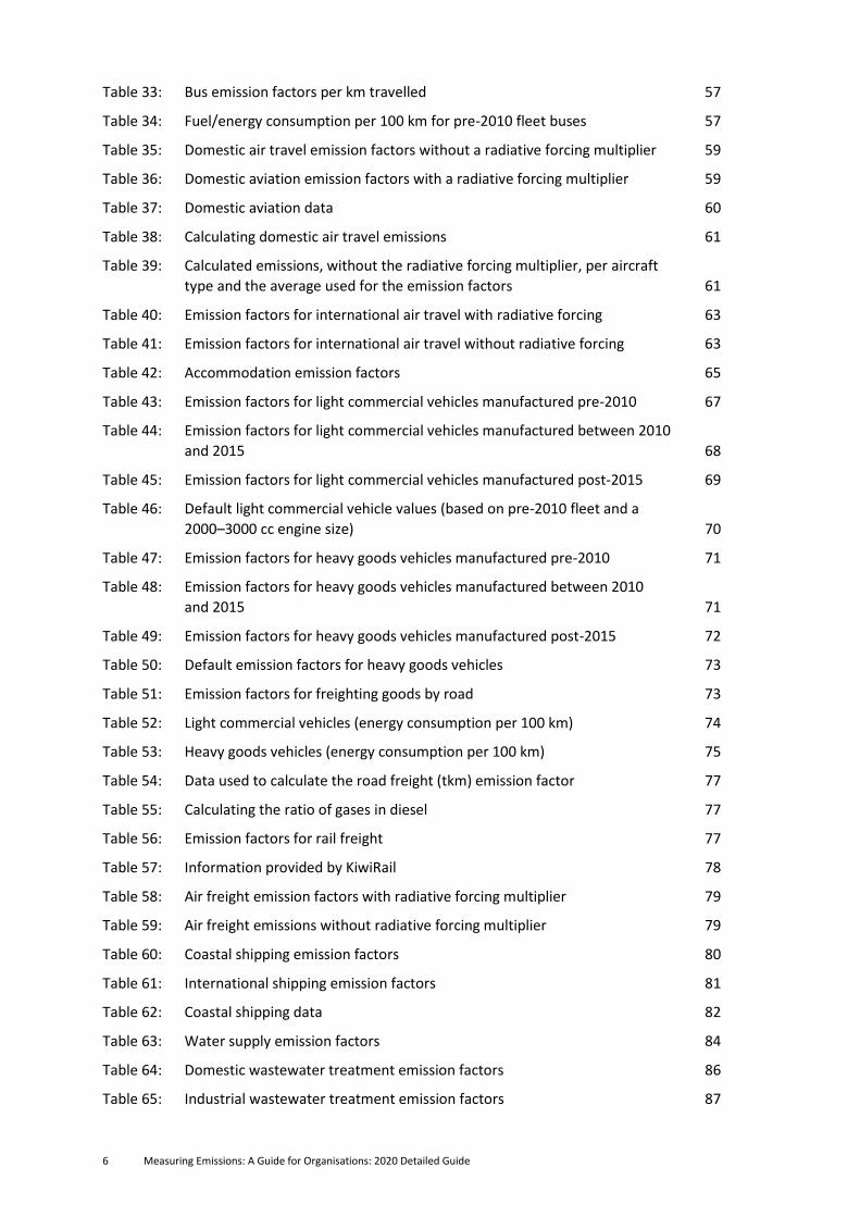
Table 33: Bus emission factors per km travelled 57
Table 34: Fuel/energy consumption per 100 km for pre-2010 fleet buses 57
Table 35: Domestic air travel emission factors without a radiative forcing multiplier 59
Table 36: Domestic aviation emission factors with a radiative forcing multiplier 59
Table 37: Domestic aviation data 60
Table 38: Calculating domestic air travel emissions 61
Table 39: Calculated emissions, without the radiative forcing multiplier, per aircraft
type and the average used for the emission factors 61
Table 40: Emission factors for international air travel with radiative forcing 63
Table 41: Emission factors for international air travel without radiative forcing 63
Table 42: Accommodation emission factors 65
Table 43: Emission factors for light commercial vehicles manufactured pre-2010 67
Table 44: Emission factors for light commercial vehicles manufactured between 2010
and 2015 68
Table 45: Emission factors for light commercial vehicles manufactured post-2015 69
Table 46: Default light commercial vehicle values (based on pre-2010 fleet and a
2000–3000 cc engine size) 70
Table 47: Emission factors for heavy goods vehicles manufactured pre-2010 71
Table 48: Emission factors for heavy goods vehicles manufactured between 2010
and 2015 71
Table 49: Emission factors for heavy goods vehicles manufactured post-2015 72
Table 50: Default emission factors for heavy goods vehicles 73
Table 51: Emission factors for freighting goods by road 73
Table 52: Light commercial vehicles (energy consumption per 100 km) 74
Table 53: Heavy goods vehicles (energy consumption per 100 km) 75
Table 54: Data used to calculate the road freight (tkm) emission factor 77
Table 55: Calculating the ratio of gases in diesel 77
Table 56: Emission factors for rail freight 77
Table 57: Information provided by KiwiRail 78
Table 58: Air freight emission factors with radiative forcing multiplier 79
Table 59: Air freight emissions without radiative forcing multiplier 79
Table 60: Coastal shipping emission factors 80
Table 61: International shipping emission factors 81
Table 62: Coastal shipping data 82
Table 63: Water supply emission factors 84
Table 64: Domestic wastewater treatment emission factors 86
Table 65: Industrial wastewater treatment emission factors 87
Measuring Emissions: A Guide for Organisations: 2020 Detailed Guide 7
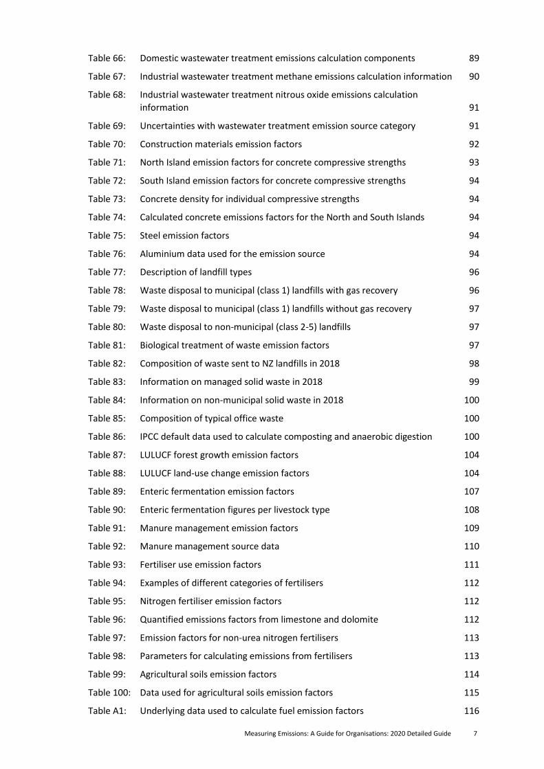
Table 66: Domestic wastewater treatment emissions calculation components 89
Table 67: Industrial wastewater treatment methane emissions calculation information 90
Table 68: Industrial wastewater treatment nitrous oxide emissions calculation
information 91
Table 69: Uncertainties with wastewater treatment emission source category 91
Table 70: Construction materials emission factors 92
Table 71: North Island emission factors for concrete compressive strengths 93
Table 72: South Island emission factors for concrete compressive strengths 94
Table 73: Concrete density for individual compressive strengths 94
Table 74: Calculated concrete emissions factors for the North and South Islands 94
Table 75: Steel emission factors 94
Table 76: Aluminium data used for the emission source 94
Table 77: Description of landfill types 96
Table 78: Waste disposal to municipal (class 1) landfills with gas recovery 96
Table 79: Waste disposal to municipal (class 1) landfills without gas recovery 97
Table 80: Waste disposal to non-municipal (class 2-5) landfills 97
Table 81: Biological treatment of waste emission factors 97
Table 82: Composition of waste sent to NZ landfills in 2018 98
Table 83: Information on managed solid waste in 2018 99
Table 84: Information on non-municipal solid waste in 2018 100
Table 85: Composition of typical office waste 100
Table 86: IPCC default data used to calculate composting and anaerobic digestion 100
Table 87: LULUCF forest growth emission factors 104
Table 88: LULUCF land-use change emission factors 104
Table 89: Enteric fermentation emission factors 107
Table 90: Enteric fermentation figures per livestock type 108
Table 91: Manure management emission factors 109
Table 92: Manure management source data 110
Table 93: Fertiliser use emission factors 111
Table 94: Examples of different categories of fertilisers 112
Table 95: Nitrogen fertiliser emission factors 112
Table 96: Quantified emissions factors from limestone and dolomite 112
Table 97: Emission factors for non-urea nitrogen fertilisers 113
Table 98: Parameters for calculating emissions from fertilisers 113
Table 99: Agricultural soils emission factors 114
Table 100: Data used for agricultural soils emission factors 115
Table A1: Underlying data used to calculate fuel emission factors 116
8 Measuring Emissions: A Guide for Organisations: 2020 Detailed Guide
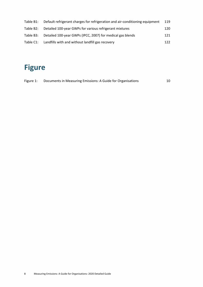
Table B1: Default refrigerant charges for refrigeration and air-conditioning equipment 119
Table B2: Detailed 100-year GWPs for various refrigerant mixtures 120
Table B3: Detailed 100-year GWPs (IPCC, 2007) for medical gas blends 121
Table C1: Landfills with and without landfill gas recovery 122
Figure
Figure 1: Documents in Measuring Emissions: A Guide for Organisations 10
Measuring Emissions: A Guide for Organisations: 2020 Detailed Guide 9
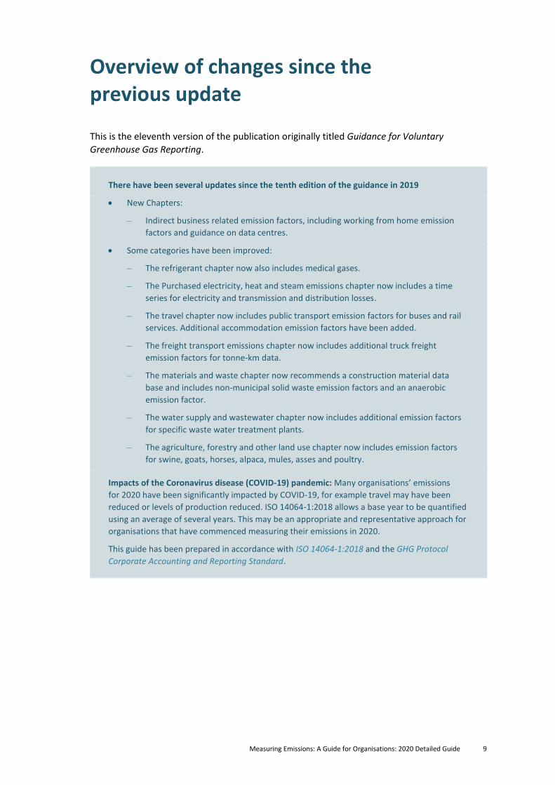
Overview of changes since the previous update
This is the eleventh version of the publication originally titled Guidance for Voluntary
Greenhouse Gas Reporting.
There have been several updates since the tenth edition of the guidance in 2019
• New Chapters:
‒ Indirect business related emission factors, including working from home emission
factors and guidance on data centres.
• Some categories have been improved:
‒ The refrigerant chapter now also includes medical gases.
‒ The Purchased electricity, heat and steam emissions chapter now includes a time
series for electricity and transmission and distribution losses.
‒ The travel chapter now includes public transport emission factors for buses and rail
services. Additional accommodation emission factors have been added.
‒ The freight transport emissions chapter now includes additional truck freight
emission factors for tonne-km data.
‒ The materials and waste chapter now recommends a construction material data
base and includes non-municipal solid waste emission factors and an anaerobic
emission factor.
‒ The water supply and wastewater chapter now includes additional emission factors
for specific waste water treatment plants.
‒ The agriculture, forestry and other land use chapter now includes emission factors
for swine, goats, horses, alpaca, mules, asses and poultry.
Impacts of the Coronavirus disease (COVID-19) pandemic: Many organisations’ emissions
for 2020 have been significantly impacted by COVID-19, for example travel may have been
reduced or levels of production reduced. ISO 14064-1:2018 allows a base year to be quantified
using an average of several years. This may be an appropriate and representative approach for
organisations that have commenced measuring their emissions in 2020.
This guide has been prepared in accordance with ISO 14064-1:2018 and the GHG Protocol
Corporate Accounting and Reporting Standard.

10 Measuring Emissions: A Guide for Organisations: 2020 Detailed Guide
1 Introduction
1.1 Purpose of this guide The Ministry for the Environment supports organisations acting on climate change. We
recognise there is strong interest from organisations across New Zealand to measure, report
and reduce their emissions. We prepared this guide to help you measure and report your
organisation’s greenhouse gas (GHG) emissions. Measuring and reporting empowers
organisations to manage and reduce emissions more effectively over time.
The guide aligns with and endorses the use of the GHG Protocol Corporate Accounting and
Reporting Standard (referred to as the GHG Protocol throughout the rest of the document) and
ISO 14064-1:2018 (see section 1.5). It provides information about preparing a GHG inventory
(section 0), emission factors (see sections 3–10, and the Emission Factors Workbook) and
methods to apply them to activity data.
We update the guide in line with international best practice and the New Zealand
Government’s Greenhouse Gas Inventory to provide new emission factors.
This Detailed Guide is part of a suite of documents that comprise Measuring Emissions: A Guide
for Organisations, listed in figure 1. The Detailed Guide explains how we derived these emission
factors and sets out the assumptions surrounding their use.
Figure 1: Documents in Measuring Emissions: A Guide for Organisations
Feedback
We welcome your feedback on this update. Please email [email protected].
Measuring Emissions: A Guide for Organisations: 2020 Detailed Guide 11
1.2 Important notes The information in this guide is intended to help organisations that want to report their GHG
emissions on a voluntary basis. This guide does not represent, or form part of, any mandatory
reporting framework or scheme.
The emission factors and methods in this guide are for sources common to many New Zealand
organisations and supports the recommended disclosure of GHG emissions consistent with the
Task Force on Climate-related Financial Disclosures (TCFD) framework. However, the complete
TCFD recommendations go beyond the scope of this guidance. For further guidance on these
please consult the TCFD website.1
The Task Force on Climate-related Financial Disclosures (TCFD) was set up by the Financial
Stability Board to increase transparency, stability, and resilience in financial markets. The TCFD
framework promotes consistent climate-related financial risk disclosures aligned with
investors’ needs and which supports organisations in understanding how to measure and
report on their climate change risks and opportunities.
In September 2020, New Zealand announced plans to introduce mandatory climate risk
reporting in line with the TCFD recommendations for all listed issuers and large banks,
investment managers and insurers. This guide and the emission factors and methods align
with the TCFD recommendations for disclosure of GHG emissions.
The emission factors and methods contained in this guide are for sources common to many
New Zealand organisations.
This guide, and the emission factors and methods, are not appropriate for a full life-cycle
assessment or product carbon footprinting. The factors presented in this guide only include
direct emissions from activities, and do not include all sources of emissions required for a full
life-cycle analysis. If you want to do a full life-cycle assessment, we recommend using UK BEIS
emission factors, which account for the life-cycle of those activities for a number of emission
sources, including well-to-tank for some categories. The GHG Protocol has also published
standards for the calculation of life-cycle emissions.2
This information is not appropriate for use in an emissions trading scheme. Organisations
required to participate in the New Zealand Emissions Trading Scheme (NZ ETS) need to comply
with the scheme-specific reporting requirements. The NZ ETS regulations determine which
emission factors and methods must be used to calculate and report emissions.
Users seeking guidance on preparing a regional inventory should refer to the GHG Protocol for
Community-scale Greenhouse Gas Emission Inventories.
If emission factors relevant to your organisation are not included in Measuring Emissions: A
Guide for Organisations, we suggest using alternatives such as those published by the UK
government: http://www.gov.uk/government/publications/greenhouse-gas-reporting-
conversion-factors-2018.
1 Task Force on Climate-related Financial Disclosures accessed via: www.fsb-tcfd.org/
2 GHG Protocol Product Standard accessed via: https://ghgprotocol.org/product-standard
12 Measuring Emissions: A Guide for Organisations: 2020 Detailed Guide
1.3 Gases included in the guide This guide covers the following greenhouse gases (GHGs): carbon dioxide (CO2), methane (CH4),
nitrous oxide (N2O), hydrofluorocarbons (HFCs), perfluorocarbons (PFCs), sulphur hexafluoride
(SF6), nitrogen trifluoride (NF3) and other gases (eg, Montreal Protocol refrigerant gases or
medical gases”.3
GHGs can trap differing amounts of heat in the atmosphere, meaning they have different
relative impacts on climate change. These are known as global warming potentials (GWPs).4
To enable a meaningful comparison between the seven gas types, GHG emissions are
commonly expressed as carbon dioxide equivalent or CO2-e. This is used throughout the guide.
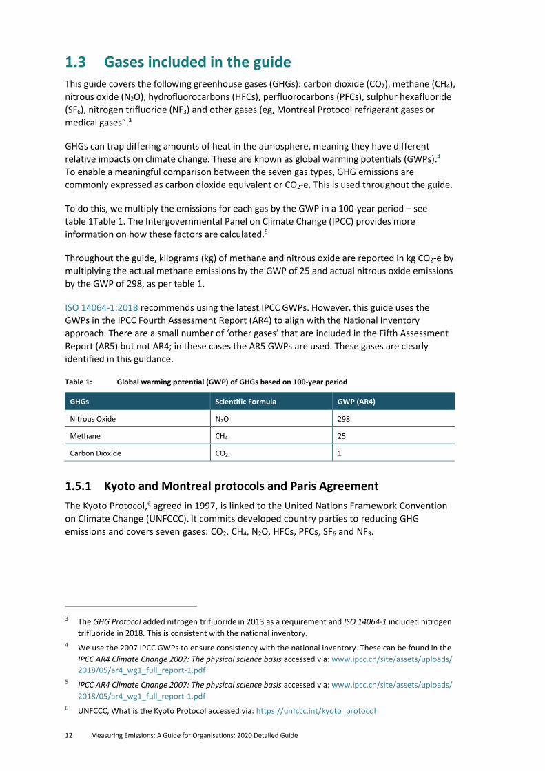
To do this, we multiply the emissions for each gas by the GWP in a 100-year period – see
table 1Table 1. The Intergovernmental Panel on Climate Change (IPCC) provides more
information on how these factors are calculated.5
Throughout the guide, kilograms (kg) of methane and nitrous oxide are reported in kg CO2-e by
multiplying the actual methane emissions by the GWP of 25 and actual nitrous oxide emissions
by the GWP of 298, as per table 1.
ISO 14064-1:2018 recommends using the latest IPCC GWPs. However, this guide uses the
GWPs in the IPCC Fourth Assessment Report (AR4) to align with the National Inventory
approach. There are a small number of ‘other gases’ that are included in the Fifth Assessment
Report (AR5) but not AR4; in these cases the AR5 GWPs are used. These gases are clearly
identified in this guidance.
Table 1: Global warming potential (GWP) of GHGs based on 100-year period
GHGs Scientific Formula GWP (AR4)
Nitrous Oxide N2O 298
Methane CH4 25
Carbon Dioxide CO2 1
1.5.1 Kyoto and Montreal protocols and Paris Agreement
The Kyoto Protocol,6 agreed in 1997, is linked to the United Nations Framework Convention
on Climate Change (UNFCCC). It commits developed country parties to reducing GHG
emissions and covers seven gases: CO2, CH4, N2O, HFCs, PFCs, SF6 and NF3.
3 The GHG Protocol added nitrogen trifluoride in 2013 as a requirement and ISO 14064-1 included nitrogen
trifluoride in 2018. This is consistent with the national inventory.
4 We use the 2007 IPCC GWPs to ensure consistency with the national inventory. These can be found in the
IPCC AR4 Climate Change 2007: The physical science basis accessed via: www.ipcc.ch/site/assets/uploads/
2018/05/ar4_wg1_full_report-1.pdf
5 IPCC AR4 Climate Change 2007: The physical science basis accessed via: www.ipcc.ch/site/assets/uploads/
2018/05/ar4_wg1_full_report-1.pdf
6 UNFCCC, What is the Kyoto Protocol accessed via: https://unfccc.int/kyoto_protocol
Measuring Emissions: A Guide for Organisations: 2020 Detailed Guide 13
The Montreal Protocol,7 agreed in 1987, is an international environmental agreement to protect the ozone layer by phasing out production and consumption of ozone-depleting substances (ODS). The Montreal Protocol includes chlorofluorocarbons (CFCs), hydrochlorofluorocarbons (HCFCs), hydrobromofluorocarbons (HBFCs), methyl bromide, carbon tetrachloride, methyl chloroform and halons. New Zealand prohibits imports of CFCs and HCFCs as part of our implementation of the protocol.
The Montreal Protocol added HFCs in 2016. The Montreal Protocol requires phasing out of HFCs and therefore has a significant role in mitigating climate change.
The 2015 Paris Agreement commits parties to put forward their best efforts to limit global temperature rise through nationally determined contributions (NDCs), and to strengthen these efforts over time. New Zealand’s inventory reporting under the Paris Agreement will be using GWPs from IPCC AR5. The first such inventory will be submitted in 2023.
1.4 Uncertainties We have used the following approach to disclose uncertainty, in order of preference.
• Disclose the data on the quantified uncertainty if known.
• Disclose the qualitative uncertainty if known based on expert judgement from those providing the data.
• Disclose the uncertainty ranges in the IPCC Guidelines if provided.
• Disclose that the uncertainty is unknown.
1.5 Standards to follow We recommend following ISO 14064-1:2018 and the GHG Protocol Corporate Accounting and
Reporting Standard. We wrote this guide to align with both.
• ISO 14064-1:20188 is shorter and more direct than the GHG Protocol. A PDF copy costs 158 Swiss francs.
• The GHG Protocol9 gives more description and context around what to do to produce an inventory. It is free to download.
Both standards provide comprehensive guidance on the core issues of GHG monitoring and
reporting at an organisational level, including:
• principles underlying monitoring and reporting
• setting organisational boundaries
• setting reporting boundaries
• establishing a base year
• managing the quality of a GHG inventory
• content of a GHG report.
7 UNDP, Montreal Protocol, accessed via: www.undp.org/content/undp/en/home/2030-agenda-for-
sustainable-development/planet/environment-and-natural-capital/chemicals-and-waste-management/ozone.html
8 Published by the International Organization for Standardization. This standard is closely based on the
GHG Protocol. 9 Developed jointly by the World Resources Institute (WRI) and the World Business Council for Sustainable
Development (WBCSD).
14 Measuring Emissions: A Guide for Organisations: 2020 Detailed Guide
1.5.1 How emission sources are categorised
The GHG Protocol places emission sources into Scope 1, Scope 2 and Scope 3 activities.
• Scope 1: Direct GHG emissions from sources owned or controlled by the company (ie, within the organisational boundary). For example, emissions from combustion of fuel in vehicles owned or controlled by the organisation.
• Scope 2: Indirect GHG emissions from the generation of purchased energy (in the form of electricity, heat or steam) that the organisation uses.
• Scope 3: Other indirect GHG emissions occurring because of the activities of the organisation but generated from sources that it does not own or control (eg, air travel).
ISO 14064-1:2018 categorises emissions as direct or indirect sources. This is to manage double
counting of emissions (such as between an electricity generator’s direct emissions associated
with generation and the indirect emissions linked to the user of that electricity). The
terminology of ‘Categories’ is used in ISO 14064-1:2018, replacing the use of ‘Scopes’.
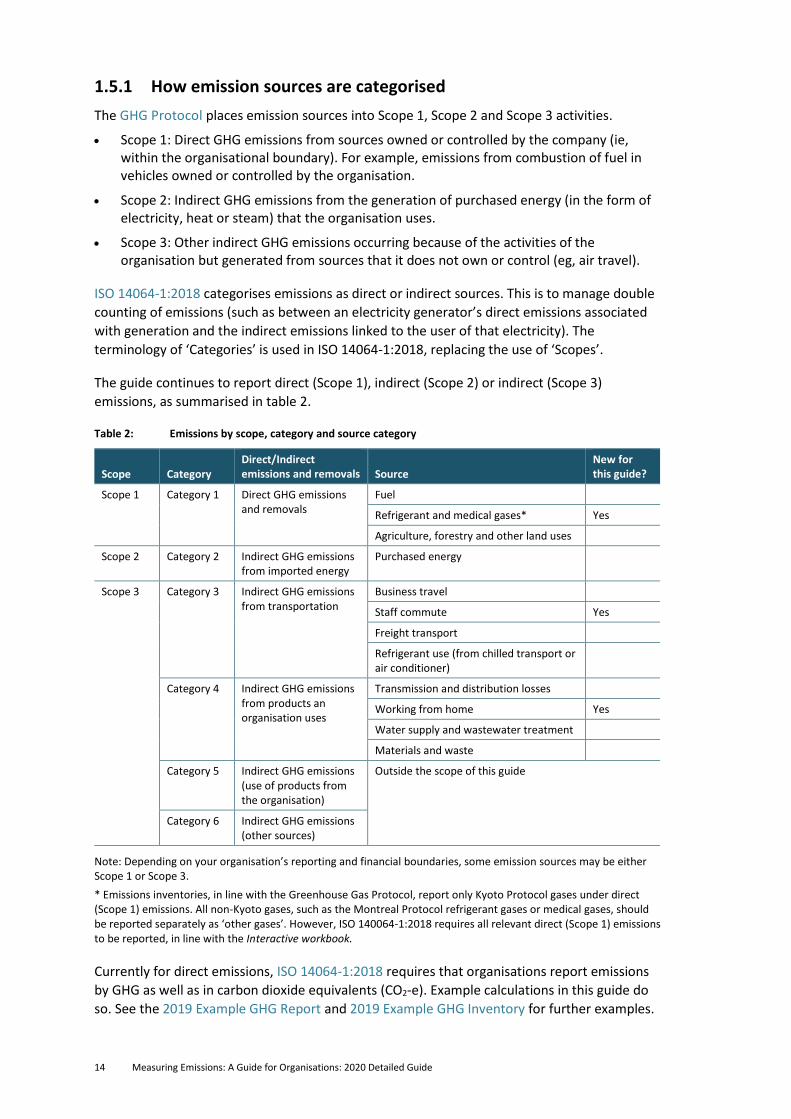
The guide continues to report direct (Scope 1), indirect (Scope 2) or indirect (Scope 3)
emissions, as summarised in table 2.
Table 2: Emissions by scope, category and source category
Scope Category Direct/Indirect emissions and removals Source
New for this guide?
Scope 1 Category 1 Direct GHG emissions and removals
Fuel
Refrigerant and medical gases* Yes
Agriculture, forestry and other land uses
Scope 2 Category 2 Indirect GHG emissions from imported energy
Purchased energy
Scope 3 Category 3 Indirect GHG emissions from transportation
Business travel
Staff commute Yes
Freight transport
Refrigerant use (from chilled transport or air conditioner)
Category 4 Indirect GHG emissions from products an organisation uses
Transmission and distribution losses
Working from home Yes
Water supply and wastewater treatment
Materials and waste
Category 5 Indirect GHG emissions (use of products from the organisation)
Outside the scope of this guide
Category 6 Indirect GHG emissions (other sources)
Note: Depending on your organisation’s reporting and financial boundaries, some emission sources may be either Scope 1 or Scope 3.
* Emissions inventories, in line with the Greenhouse Gas Protocol, report only Kyoto Protocol gases under direct (Scope 1) emissions. All non-Kyoto gases, such as the Montreal Protocol refrigerant gases or medical gases, should be reported separately as ‘other gases’. However, ISO 140064-1:2018 requires all relevant direct (Scope 1) emissions to be reported, in line with the Interactive workbook.
Currently for direct emissions, ISO 14064-1:2018 requires that organisations report emissions
by GHG as well as in carbon dioxide equivalents (CO2-e). Example calculations in this guide do
so. See the 2019 Example GHG Report and 2019 Example GHG Inventory for further examples.
Measuring Emissions: A Guide for Organisations: 2020 Detailed Guide 15
2 How to quantify and report GHG emissions
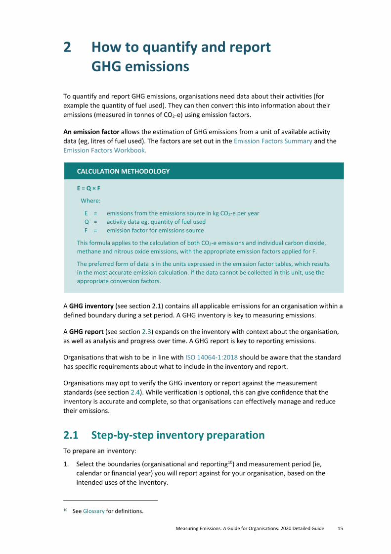
To quantify and report GHG emissions, organisations need data about their activities (for
example the quantity of fuel used). They can then convert this into information about their
emissions (measured in tonnes of CO2-e) using emission factors.
An emission factor allows the estimation of GHG emissions from a unit of available activity
data (eg, litres of fuel used). The factors are set out in the Emission Factors Summary and the
Emission Factors Workbook.
CALCULATION METHODOLOGY
E = Q × F
Where:
E = emissions from the emissions source in kg CO2-e per year
Q = activity data eg, quantity of fuel used
F = emission factor for emissions source
This formula applies to the calculation of both CO2-e emissions and individual carbon dioxide,
methane and nitrous oxide emissions, with the appropriate emission factors applied for F.
The preferred form of data is in the units expressed in the emission factor tables, which results
in the most accurate emission calculation. If the data cannot be collected in this unit, use the
appropriate conversion factors.
A GHG inventory (see section 2.1) contains all applicable emissions for an organisation within a
defined boundary during a set period. A GHG inventory is key to measuring emissions.
A GHG report (see section 2.3) expands on the inventory with context about the organisation,
as well as analysis and progress over time. A GHG report is key to reporting emissions.
Organisations that wish to be in line with ISO 14064-1:2018 should be aware that the standard
has specific requirements about what to include in the inventory and report.
Organisations may opt to verify the GHG inventory or report against the measurement
standards (see section 2.4). While verification is optional, this can give confidence that the
inventory is accurate and complete, so that organisations can effectively manage and reduce
their emissions.
2.1 Step-by-step inventory preparation To prepare an inventory:
1. Select the boundaries (organisational and reporting10) and measurement period (ie,
calendar or financial year) you will report against for your organisation, based on the
intended uses of the inventory.
10 See Glossary for definitions.
16 Measuring Emissions: A Guide for Organisations: 2020 Detailed Guide
2. Collect activity data on each emission source within the boundaries for that period.
3. Multiply the quantity used by the appropriate emission factor in a spreadsheet. See the
2019 Example GHG Inventory.
4. Produce a GHG report, if applicable. See section 2.3 and the 2019 Example GHG Report.
If this is the first year your organisation has produced an inventory, you can use it as a base
year for measuring the change in emissions over time (as long as the scope and boundaries
represent your usual operations, and that comparable reporting is used in future years). ISO
14064-1:2018 also allows a base year to be quantified using an average of several years. Due to
Covid-19 this may be an appropriate and representative approach for organisations that have
commenced measuring their emissions in 2020.
For some organisations, certain GHG emissions may contribute such a small portion of the
inventory that they make up less than 1 per cent of the total inventory. These are known as
de minimis11 and may be excluded from the total inventory, provided that the total of excluded
emissions does not exceed the materiality threshold. For example, if using a materiality
threshold of 5 per cent, the total of all emission sources excluded as de minimis must not
exceed 5 per cent of the inventory. Typically, an organisation estimates any emissions
considered de minimis using simplified methods to justify the classification. It is important
these are transparently documented and justified. You only need to re-estimate excluded
emissions in subsequent years if the assumptions change.
2.2 Using the emission factors Emission factors rely on historical data. This 2020 guide is based on New Zealand’s Greenhouse
Gas Inventory 1990–2018 as this was the latest complete set of data available. We intend to
update these emissions factors every second year, where more recent data is available.
If you use the Interactive Workbook, input your activity data and the emission factors
will be applied automatically. If you do not use the Interactive Workbook, simplified
example calculations are provided throughout chapter 4 to demonstrate how to use the
emission factors.12
Organisations can choose to report on a calendar- or financial-year basis. The chosen period
determines which historical factors to use.
Calendar year: If you are reporting on a calendar-year basis, use the latest published emission
factors. For example, if you are reporting emissions for the 2019 calendar year, use this 2020
guide, which largely relies on 2018 data.
Financial year: If you are reporting on a financial-year basis, use the guide that the greatest
portion of your data falls within. For example, if you are reporting for the 2019/2020 financial
year, use this 2020 guide. For a July to June reporting year, apply the more recent set of factors.
11 See Glossary for definition.
12 Note that the emission factors in the example calculations within this document, the Emission Factors
Summary and the Emission Factors Workbook are rounded. In the Interactive Workbook they are not. For
this reason, you may notice small discrepancies between the answers in the example calculations and the
answers provided in the Interactive Workbook.
Measuring Emissions: A Guide for Organisations: 2020 Detailed Guide 17
The emission factors in this guide are:
• default factors, used in the absence of better company- or industry-specific information
• consistent with the reporting requirements of ISO 14064-1:2018 and the GHG Protocol
• aligned with New Zealand’s Greenhouse Gas Inventory 1990-2018. This also means we use the GWPs from the AR4 to ensure consistency.
Under the reporting requirements of ISO 14064-1:2018 and the GHG Protocol, GHG emissions
should be reported in tonnes CO2-e. However, many emission factors are too small to be
reported meaningfully in tonnes, therefore this guide presents emission factors in kg CO2-e per
unit. Dividing by 1000 converts kg to tonnes (see example calculations on the following pages).
In line with the reporting requirements of ISO 14064-1:2018, the emission factors allow
calculation of carbon dioxide, methane and nitrous oxide separately, as well as the total
carbon dioxide equivalent for direct (Scope 1) emission sources.
Carbon dioxide emission factors are based on the carbon and energy content of a fuel.
Therefore, the carbon dioxide emissions remain constant irrespective of how a fuel is
combusted.
Non-carbon dioxide emissions (ie, methane and nitrous oxide) and emission factors depend
on the way the fuel is combusted.13 To reflect this variability, the guide provides uncertainty
estimates for direct (Scope 1) emission factors. Table 3 presents separate carbon dioxide
equivalent emission factors for residential, commercial and industrial users. It follows the
IPCC guidelines for combustion and adopts the uncertainties.14
We mainly derived these emission factors from technical information published by
New Zealand government agencies. Each section below provides the source for each
emission factor and describes how we derived the factors.
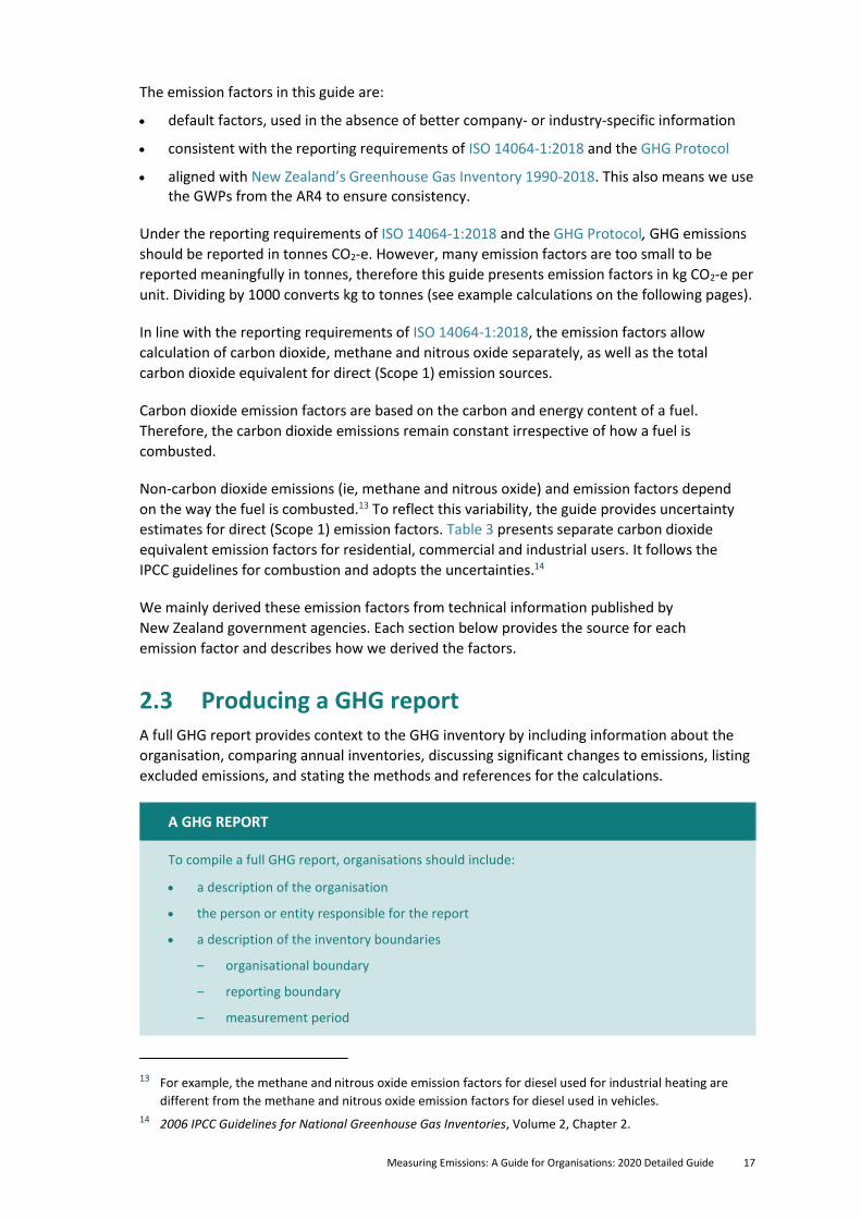
2.3 Producing a GHG report A full GHG report provides context to the GHG inventory by including information about the
organisation, comparing annual inventories, discussing significant changes to emissions, listing
excluded emissions, and stating the methods and references for the calculations.
A GHG REPORT
To compile a full GHG report, organisations should include:
• a description of the organisation
• the person or entity responsible for the report
• a description of the inventory boundaries
‒ organisational boundary
‒ reporting boundary
‒ measurement period
13 For example, the methane and nitrous oxide emission factors for diesel used for industrial heating are
different from the methane and nitrous oxide emission factors for diesel used in vehicles.
14 2006 IPCC Guidelines for National Greenhouse Gas Inventories, Volume 2, Chapter 2.

18 Measuring Emissions: A Guide for Organisations: 2020 Detailed Guide
A GHG REPORT
• the chosen base year (initial measurement period for comparing annual results)
• emissions (and removals where appropriate)
• for all seven GHGs separately in metric tonnes CO2-e
• emissions separated by scope
‒ total Scope 1 and 2 emissions
‒ specified Scope 3 emissions
• emissions from biologically sequestered carbon reported separately from the scopes
• a time series of emissions results from base year to present year
• significant emissions changes, including in the context of triggering any base year
recalculations
• the methodologies for calculating emissions, and references to key data sources
• impacts of uncertainty on the inventory
• any specific exclusions of sources, facilities or operations.
View an example reporting template on the GHG Protocol Corporate Standard webpage.
2.4 Verification Verification15 gives confidence about the GHG inventory and report. If you intend to publicly
release the inventory, we recommend it is independently verified to confirm calculations are
accurate, the inventory is complete and you have followed the correct methodologies.
2.4.1 Who should verify my inventory?
If you opt for verification, we recommend using verifiers who:
• are independent
• are members of a suitable professional organisation
• have experience with emissions inventories
• understand ISO 14064 and the GHG Protocol
• have effective internal peer review and quality control processes.
To help organisations assess a verifier’s qualifications, users may choose to use an accredited
body. For example, accreditation under the ISO 14065 standard confirms that verifiers are
suitably qualified and enables them to certify an inventory as being prepared in accordance
with ISO 14064-1:2018.
15 See
Glossary for definition.

Measuring Emissions: A Guide for Organisations: 2020 Detailed Guide 19
In New Zealand, the Joint Accreditation System of Australia and New Zealand (JAS-ANZ) issues
accreditations and publishes a list of accredited bodies on its website.16
16 View accredited bodies on the JAS-ANZ Register at www.jas-anz.org/accredited-bodies/all
20 Measuring Emissions: A Guide for Organisations: 2020 Detailed Guide
3 Fuel emission factors
Fuel can be categorised as stationary combustion or transport. This section also includes
biofuels, and the transmission and distribution losses for reticulated natural gas.
In line with the reporting requirements of ISO 14064-1:2018 and the GHG Protocol, we provide
emission factors for direct (Scope 1) sources to allow separate carbon dioxide, methane and
nitrous oxide calculations.
3.1 Overview of changes since previous update There has been no update to emission factors for stationary fuels, transport fuels, biofuels
and biomass.
3.2 Stationary combustion fuel Stationary combustion fuels are burnt in a fixed unit or asset, such as a boiler. Direct (Scope 1)
emissions occur from the combustion of fuels from sources owned or controlled by the
reporting organisation. If the organisation does not own or control the assets where
combustion takes place, then these emissions are indirect (Scope 3) emissions. For more
information see section 1.5.1.
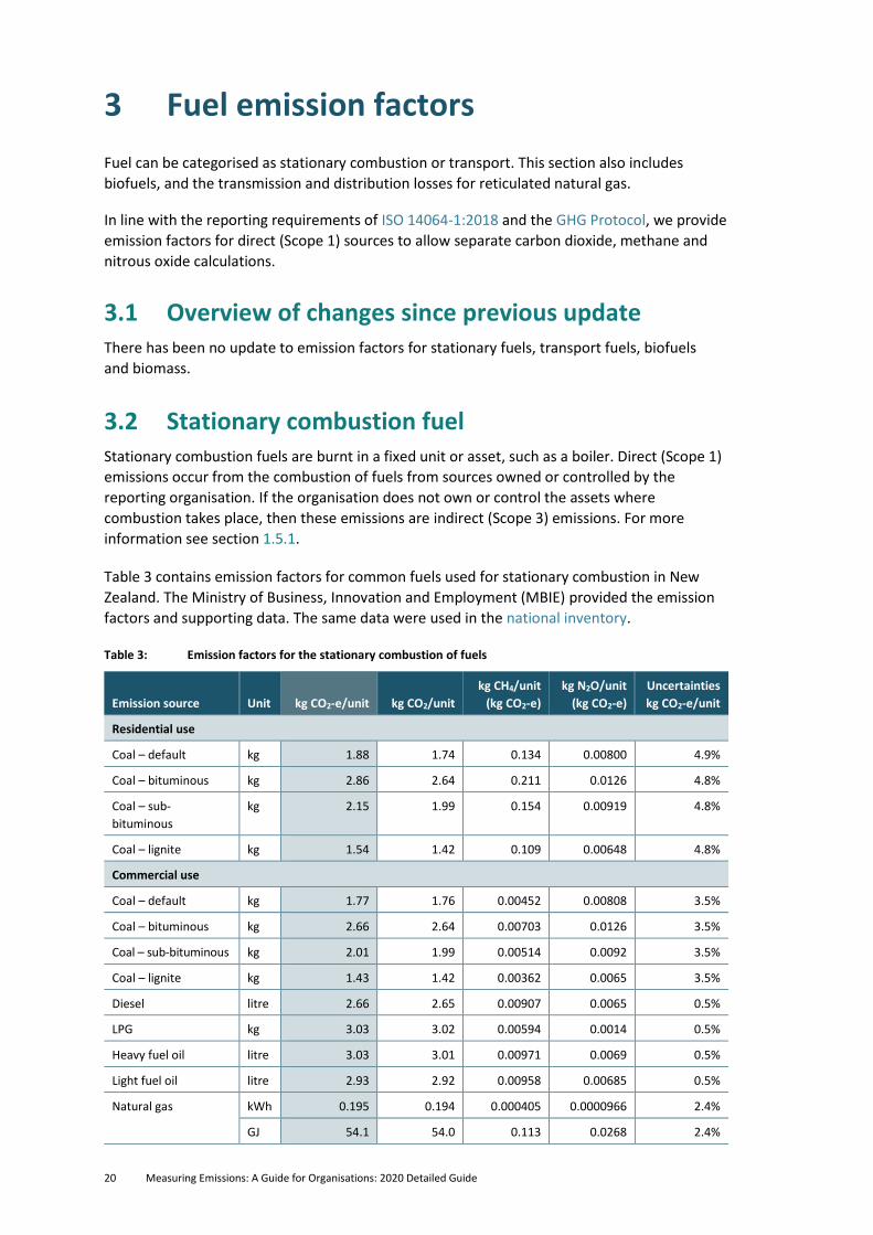
Table 3 contains emission factors for common fuels used for stationary combustion in New
Zealand. The Ministry of Business, Innovation and Employment (MBIE) provided the emission
factors and supporting data. The same data were used in the national inventory.
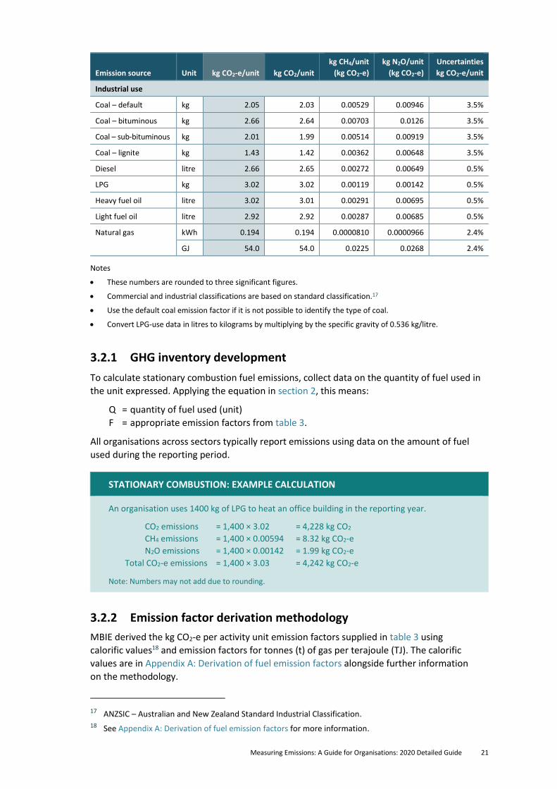
Table 3: Emission factors for the stationary combustion of fuels
Emission source Unit kg CO2-e/unit kg CO2/unit
kg CH4/unit
(kg CO2-e)
kg N2O/unit
(kg CO2-e)
Uncertainties
kg CO2-e/unit
Residential use
Coal – default kg 1.88 1.74 0.134 0.00800 4.9%
Coal – bituminous kg 2.86 2.64 0.211 0.0126 4.8%
Coal – sub-
bituminous
kg 2.15 1.99 0.154 0.00919 4.8%
Coal – lignite kg 1.54 1.42 0.109 0.00648 4.8%
Commercial use
Coal – default kg 1.77 1.76 0.00452 0.00808 3.5%
Coal – bituminous kg 2.66 2.64 0.00703 0.0126 3.5%
Coal – sub-bituminous kg 2.01 1.99 0.00514 0.0092 3.5%
Coal – lignite kg 1.43 1.42 0.00362 0.0065 3.5%
Diesel litre 2.66 2.65 0.00907 0.0065 0.5%
LPG kg 3.03 3.02 0.00594 0.0014 0.5%
Heavy fuel oil litre 3.03 3.01 0.00971 0.0069 0.5%
Light fuel oil litre 2.93 2.92 0.00958 0.00685 0.5%
Natural gas kWh 0.195 0.194 0.000405 0.0000966 2.4%
GJ 54.1 54.0 0.113 0.0268 2.4%
Measuring Emissions: A Guide for Organisations: 2020 Detailed Guide 21
Emission source Unit kg CO2-e/unit kg CO2/unit
kg CH4/unit
(kg CO2-e)
kg N2O/unit
(kg CO2-e)
Uncertainties
kg CO2-e/unit
Industrial use
Coal – default kg 2.05 2.03 0.00529 0.00946 3.5%
Coal – bituminous kg 2.66 2.64 0.00703 0.0126 3.5%
Coal – sub-bituminous kg 2.01 1.99 0.00514 0.00919 3.5%
Coal – lignite kg 1.43 1.42 0.00362 0.00648 3.5%
Diesel litre 2.66 2.65 0.00272 0.00649 0.5%
LPG kg 3.02 3.02 0.00119 0.00142 0.5%
Heavy fuel oil litre 3.02 3.01 0.00291 0.00695 0.5%
Light fuel oil litre 2.92 2.92 0.00287 0.00685 0.5%
Natural gas kWh 0.194 0.194 0.0000810 0.0000966 2.4%
GJ 54.0 54.0 0.0225 0.0268 2.4%
Notes
• These numbers are rounded to three significant figures.
• Commercial and industrial classifications are based on standard classification.17
• Use the default coal emission factor if it is not possible to identify the type of coal.
• Convert LPG-use data in litres to kilograms by multiplying by the specific gravity of 0.536 kg/litre.
3.2.1 GHG inventory development
To calculate stationary combustion fuel emissions, collect data on the quantity of fuel used in
the unit expressed. Applying the equation in section 2, this means:
Q = quantity of fuel used (unit)
F = appropriate emission factors from table 3.
All organisations across sectors typically report emissions using data on the amount of fuel
used during the reporting period.
STATIONARY COMBUSTION: EXAMPLE CALCULATION
An organisation uses 1400 kg of LPG to heat an office building in the reporting year.
CO2 emissions = 1,400 × 3.02 = 4,228 kg CO2
CH4 emissions = 1,400 × 0.00594 = 8.32 kg CO2-e
N2O emissions = 1,400 × 0.00142 = 1.99 kg CO2-e
Total CO2-e emissions = 1,400 × 3.03 = 4,242 kg CO2-e
Note: Numbers may not add due to rounding.
3.2.2 Emission factor derivation methodology
MBIE derived the kg CO2-e per activity unit emission factors supplied in table 3 using
calorific values18 and emission factors for tonnes (t) of gas per terajoule (TJ). The calorific
values are in Appendix A: Derivation of fuel emission factors alongside further information
on the methodology.
17 ANZSIC – Australian and New Zealand Standard Industrial Classification. 18 See Appendix A: Derivation of fuel emission factors for more information.
22 Measuring Emissions: A Guide for Organisations: 2020 Detailed Guide
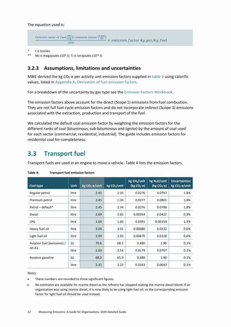
The equation used is:
𝐶𝑎𝑙𝑜𝑟𝑖𝑓𝑖𝑐 𝑣𝑎𝑙𝑢𝑒 𝑜𝑓 𝑓𝑢𝑒𝑙 (𝑀𝐽
𝑘𝑔)× 𝑒𝑚𝑖𝑠𝑠𝑖𝑜𝑛 𝑓𝑎𝑐𝑡𝑜𝑟 (
𝑡 𝑔𝑎𝑠
𝑇𝐽)
1000= 𝑒𝑚𝑖𝑠𝑠𝑖𝑜𝑛 𝑓𝑎𝑐𝑡𝑜𝑟 𝑘𝑔 𝑔𝑎𝑠/𝑘𝑔 𝑓𝑢𝑒𝑙
* t is tonnes
** MJ is megajoules (106 J); TJ is terajoules (1012 J)
3.2.3 Assumptions, limitations and uncertainties
MBIE derived the kg CO2-e per activity unit emission factors supplied in table 3 using calorific
values, listed in Appendix A: Derivation of fuel emission factors.
For a breakdown of the uncertainty by gas type see the Emission Factors Workbook.
The emission factors above account for the direct (Scope 1) emissions from fuel combustion.
They are not full fuel-cycle emission factors and do not incorporate indirect (Scope 3) emissions
associated with the extraction, production and transport of the fuel.
We calculated the default coal emission factor by weighting the emission factors for the
different ranks of coal (bituminous, sub-bituminous and lignite) by the amount of coal used
for each sector (commercial, residential, industrial). The guide includes emission factors for
residential coal for completeness.
3.3 Transport fuel Transport fuels are used in an engine to move a vehicle. Table 4 lists the emission factors.
Table 4: Transport fuel emission factors
Fuel type Unit kg CO2-e/unit kg CO2/unit
kg CH4/unit
(kg CO2-e)
kg N2O/unit
(kg CO2-e)
Uncertainties
kg CO2-e/unit
Regular petrol litre 2.45 2.35 0.0276 0.0797 1.8%
Premium petrol litre 2.45 2.34 0.0277 0.0801 1.8%
Petrol – default* litre 2.45 2.34 0.0276 0.0798 1.8%
Diesel litre 2.69 2.65 0.00354 0.0422 0.9%
LPG litre 1.64 1.60 0.0391 0.00150 1.3%
Heavy fuel oil litre 3.04 3.01 0.00680 0.0232 0.6%
Light fuel oil litre 2.94 2.92 0.00670 0.0228 0.6%
Aviation fuel (kerosene) /
Jet A1
GJ 70.6 68.2 0.480 1.90 0.1%
litre 2.63 2.54 0.0179 0.0707 0.1%
Aviation gasoline GJ 68.3 65.9 0.480 1.90 0.1%
litre 2.31 2.23 0.0163 0.0643 0.1%
Notes:
• These numbers are rounded to three significant figures.
• No estimates are available for marine diesel as the refinery has stopped making the marine diesel blend. If an
organisation was using marine diesel, it is now likely to be using light fuel oil; so the corresponding emission
factor for light fuel oil should be used instead.
Measuring Emissions: A Guide for Organisations: 2020 Detailed Guide 23
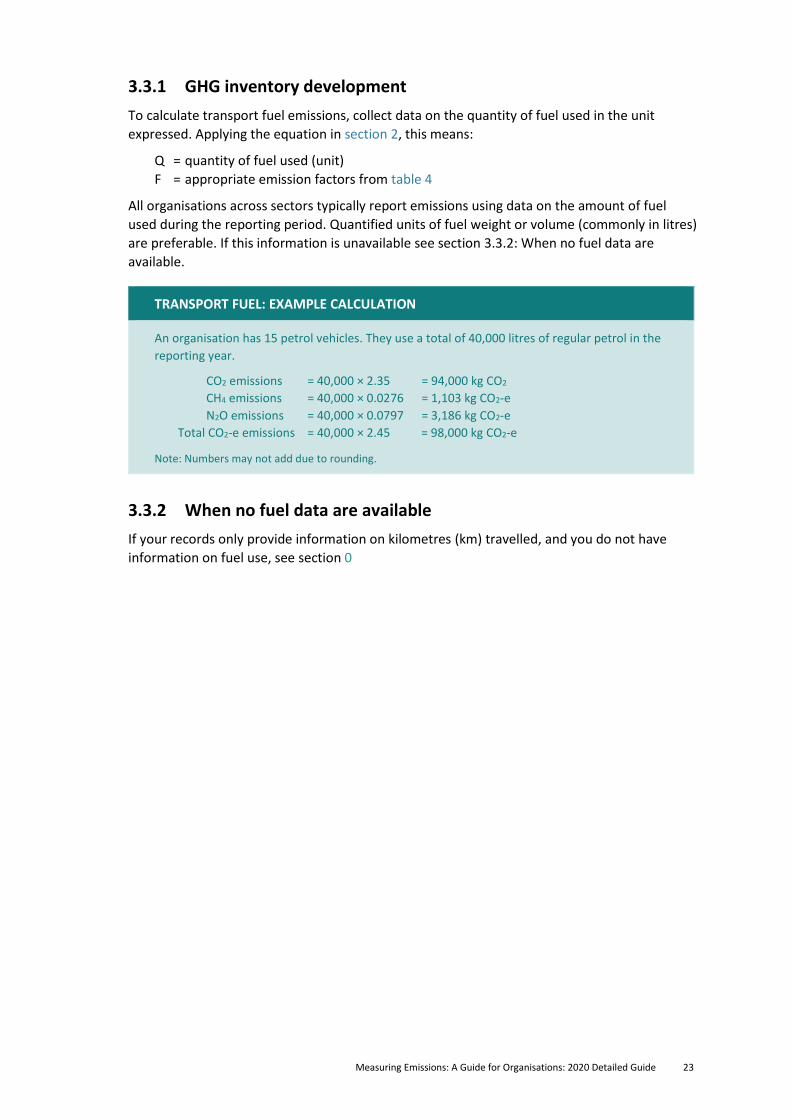
3.3.1 GHG inventory development
To calculate transport fuel emissions, collect data on the quantity of fuel used in the unit
expressed. Applying the equation in section 2, this means:
Q = quantity of fuel used (unit)
F = appropriate emission factors from table 4
All organisations across sectors typically report emissions using data on the amount of fuel
used during the reporting period. Quantified units of fuel weight or volume (commonly in litres)
are preferable. If this information is unavailable see section 3.3.2: When no fuel data are
available.
TRANSPORT FUEL: EXAMPLE CALCULATION
An organisation has 15 petrol vehicles. They use a total of 40,000 litres of regular petrol in the
reporting year.
CO2 emissions = 40,000 × 2.35 = 94,000 kg CO2
CH4 emissions = 40,000 × 0.0276 = 1,103 kg CO2-e
N2O emissions = 40,000 × 0.0797 = 3,186 kg CO2-e
Total CO2-e emissions = 40,000 × 2.45 = 98,000 kg CO2-e
Note: Numbers may not add due to rounding.
3.3.2 When no fuel data are available
If your records only provide information on kilometres (km) travelled, and you do not have
information on fuel use, see section 0
24 Measuring Emissions: A Guide for Organisations: 2020 Detailed Guide
Travel emission factors. Factors such as individual vehicle fuel efficiency and driving efficiency
mean that kilometre-based estimates of carbon dioxide equivalent emissions are less accurate
than calculating emissions based on fuel-use data. Therefore, only use the emission factors
based on distance travelled if information on fuel use is not available.
Calculating transport fuel based on dollars spent is less accurate and should only be applied to
taxis. See section 7.2.
3.3.3 Emission factor derivation methodology
We applied the same methodology to the transport fuels that we used to calculate the
stationary combustion fuels, using the raw data in table 4.
3.3.4 Assumptions, limitations and uncertainties
MBIE derived the kg CO2-e per activity unit emission factors in table 3 using calorific values. All
emission factors incorporate relevant oxidation factors sourced from the 2006 IPCC Guidelines
for National Greenhouse Gas Inventories.
The default petrol factor has not been updated since the last emissions factor publication and is
a weighted average of regular and premium petrol based on 2016 sales volume data from
Energy in New Zealand 2016 (MBIE, 2016). Use this default factor when petrol-use data do not
distinguish between regular and premium petrol.
As with the fuels for stationary combustion, these emission factors are not full fuel-cycle
emission factors and do not incorporate the indirect (Scope 3) emissions associated with the
extraction, production and transport of the fuel.
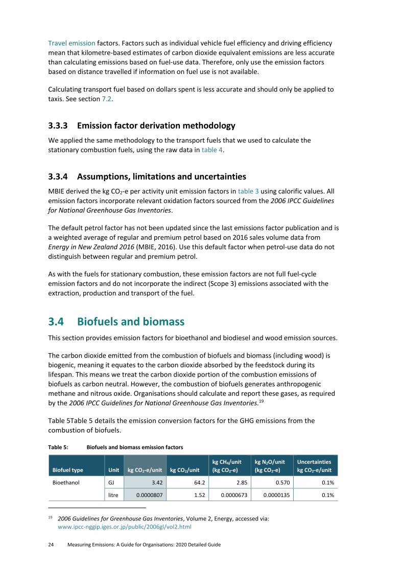
3.4 Biofuels and biomass This section provides emission factors for bioethanol and biodiesel and wood emission sources.
The carbon dioxide emitted from the combustion of biofuels and biomass (including wood) is
biogenic, meaning it equates to the carbon dioxide absorbed by the feedstock during its
lifespan. This means we treat the carbon dioxide portion of the combustion emissions of
biofuels as carbon neutral. However, the combustion of biofuels generates anthropogenic
methane and nitrous oxide. Organisations should calculate and report these gases, as required
by the 2006 IPCC Guidelines for National Greenhouse Gas Inventories.19
Table 5Table 5 details the emission conversion factors for the GHG emissions from the
combustion of biofuels.
Table 5: Biofuels and biomass emission factors
Biofuel type Unit kg CO2-e/unit kg CO2/unit
kg CH4/unit
(kg CO2-e)
kg N2O/unit
(kg CO2-e)
Uncertainties
kg CO2-e/unit
Bioethanol GJ 3.42 64.2 2.85 0.570 0.1%
litre 0.0000807 1.52 0.0000673 0.0000135 0.1%
19 2006 Guidelines for Greenhouse Gas Inventories, Volume 2, Energy, accessed via:
www.ipcc-nggip.iges.or.jp/public/2006gl/vol2.html
Measuring Emissions: A Guide for Organisations: 2020 Detailed Guide 25
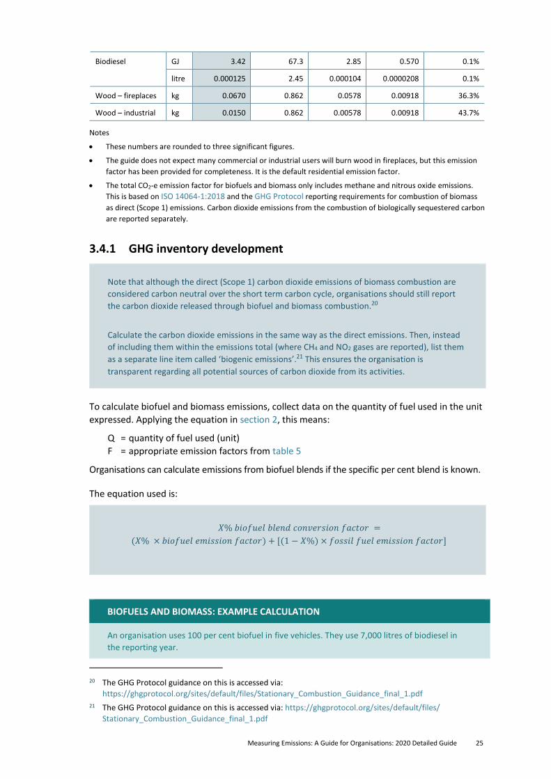
Biodiesel GJ 3.42 67.3 2.85 0.570 0.1%
litre 0.000125 2.45 0.000104 0.0000208 0.1%
Wood – fireplaces kg 0.0670 0.862 0.0578 0.00918 36.3%
Wood – industrial kg 0.0150 0.862 0.00578 0.00918 43.7%
Notes
• These numbers are rounded to three significant figures.
• The guide does not expect many commercial or industrial users will burn wood in fireplaces, but this emission
factor has been provided for completeness. It is the default residential emission factor.
• The total CO2-e emission factor for biofuels and biomass only includes methane and nitrous oxide emissions.
This is based on ISO 14064-1:2018 and the GHG Protocol reporting requirements for combustion of biomass
as direct (Scope 1) emissions. Carbon dioxide emissions from the combustion of biologically sequestered carbon
are reported separately.
3.4.1 GHG inventory development
Note that although the direct (Scope 1) carbon dioxide emissions of biomass combustion are
considered carbon neutral over the short term carbon cycle, organisations should still report
the carbon dioxide released through biofuel and biomass combustion.20
Calculate the carbon dioxide emissions in the same way as the direct emissions. Then, instead
of including them within the emissions total (where CH4 and NO2 gases are reported), list them
as a separate line item called ‘biogenic emissions’.21 This ensures the organisation is
transparent regarding all potential sources of carbon dioxide from its activities.
To calculate biofuel and biomass emissions, collect data on the quantity of fuel used in the unit
expressed. Applying the equation in section 2, this means:
Q = quantity of fuel used (unit)
F = appropriate emission factors from table 5
Organisations can calculate emissions from biofuel blends if the specific per cent blend is known.
The equation used is:
𝑋% 𝑏𝑖𝑜𝑓𝑢𝑒𝑙 𝑏𝑙𝑒𝑛𝑑 𝑐𝑜𝑛𝑣𝑒𝑟𝑠𝑖𝑜𝑛 𝑓𝑎𝑐𝑡𝑜𝑟 =
(𝑋% × 𝑏𝑖𝑜𝑓𝑢𝑒𝑙 𝑒𝑚𝑖𝑠𝑠𝑖𝑜𝑛 𝑓𝑎𝑐𝑡𝑜𝑟) + [(1 − 𝑋%) × 𝑓𝑜𝑠𝑠𝑖𝑙 𝑓𝑢𝑒𝑙 𝑒𝑚𝑖𝑠𝑠𝑖𝑜𝑛 𝑓𝑎𝑐𝑡𝑜𝑟]
BIOFUELS AND BIOMASS: EXAMPLE CALCULATION
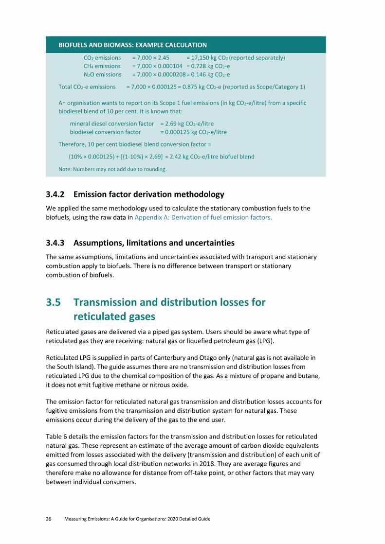
An organisation uses 100 per cent biofuel in five vehicles. They use 7,000 litres of biodiesel in
the reporting year.
20 The GHG Protocol guidance on this is accessed via:
https://ghgprotocol.org/sites/default/files/Stationary_Combustion_Guidance_final_1.pdf
21 The GHG Protocol guidance on this is accessed via: https://ghgprotocol.org/sites/default/files/
Stationary_Combustion_Guidance_final_1.pdf
26 Measuring Emissions: A Guide for Organisations: 2020 Detailed Guide
BIOFUELS AND BIOMASS: EXAMPLE CALCULATION
CO2 emissions = 7,000 × 2.45 = 17,150 kg CO2 (reported separately)
CH4 emissions = 7,000 × 0.000104 = 0.728 kg CO2-e
N2O emissions = 7,000 × 0.0000208 = 0.146 kg CO2-e
Total CO2-e emissions = 7,000 × 0.000125 = 0.875 kg CO2-e (reported as Scope/Category 1)
An organisation wants to report on its Scope 1 fuel emissions (in kg CO2-e/litre) from a specific
biodiesel blend of 10 per cent. It is known that:
mineral diesel conversion factor = 2.69 kg CO2-e/litre
biodiesel conversion factor = 0.000125 kg CO2-e/litre
Therefore, 10 per cent biodiesel blend conversion factor =
(10% × 0.000125) + [(1-10%) × 2.69] = 2.42 kg CO2-e/litre biofuel blend
Note: Numbers may not add due to rounding.
3.4.2 Emission factor derivation methodology
We applied the same methodology used to calculate the stationary combustion fuels to the
biofuels, using the raw data in Appendix A: Derivation of fuel emission factors.
3.4.3 Assumptions, limitations and uncertainties
The same assumptions, limitations and uncertainties associated with transport and stationary
combustion apply to biofuels. There is no difference between transport or stationary
combustion of biofuels.
3.5 Transmission and distribution losses for reticulated gases
Reticulated gases are delivered via a piped gas system. Users should be aware what type of
reticulated gas they are receiving: natural gas or liquefied petroleum gas (LPG).
Reticulated LPG is supplied in parts of Canterbury and Otago only (natural gas is not available in
the South Island). The guide assumes there are no transmission and distribution losses from
reticulated LPG due to the chemical composition of the gas. As a mixture of propane and butane,
it does not emit fugitive methane or nitrous oxide.
The emission factor for reticulated natural gas transmission and distribution losses accounts for
fugitive emissions from the transmission and distribution system for natural gas. These
emissions occur during the delivery of the gas to the end user.
Table 6 details the emission factors for the transmission and distribution losses for reticulated
natural gas. These represent an estimate of the average amount of carbon dioxide equivalents
emitted from losses associated with the delivery (transmission and distribution) of each unit of
gas consumed through local distribution networks in 2018. They are average figures and
therefore make no allowance for distance from off-take point, or other factors that may vary
between individual consumers.
Measuring Emissions: A Guide for Organisations: 2020 Detailed Guide 27
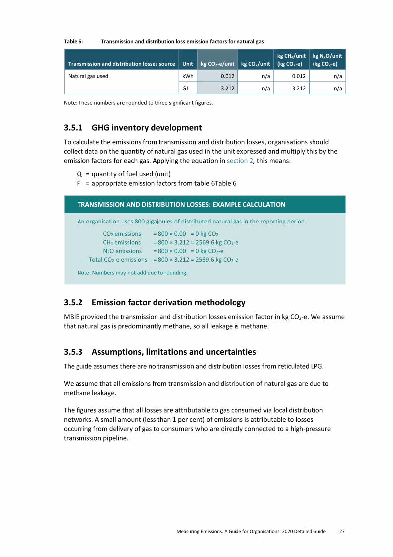
Table 6: Transmission and distribution loss emission factors for natural gas
Transmission and distribution losses source Unit kg CO2-e/unit kg CO2/unit
kg CH4/unit
(kg CO2-e)
kg N2O/unit
(kg CO2-e)
Natural gas used kWh 0.012 n/a 0.012 n/a
GJ 3.212 n/a 3.212 n/a
Note: These numbers are rounded to three significant figures.
3.5.1 GHG inventory development
To calculate the emissions from transmission and distribution losses, organisations should
collect data on the quantity of natural gas used in the unit expressed and multiply this by the
emission factors for each gas. Applying the equation in section 2, this means:
Q = quantity of fuel used (unit)
F = appropriate emission factors from table 6Table 6
TRANSMISSION AND DISTRIBUTION LOSSES: EXAMPLE CALCULATION
An organisation uses 800 gigajoules of distributed natural gas in the reporting period.
CO2 emissions = 800 × 0.00 = 0 kg CO2
CH4 emissions = 800 × 3.212 = 2569.6 kg CO2-e
N2O emissions = 800 × 0.00 = 0 kg CO2-e
Total CO2-e emissions = 800 × 3.212 = 2569.6 kg CO2-e
Note: Numbers may not add due to rounding.
3.5.2 Emission factor derivation methodology
MBIE provided the transmission and distribution losses emission factor in kg CO2-e. We assume
that natural gas is predominantly methane, so all leakage is methane.
3.5.3 Assumptions, limitations and uncertainties
The guide assumes there are no transmission and distribution losses from reticulated LPG.
We assume that all emissions from transmission and distribution of natural gas are due to
methane leakage.
The figures assume that all losses are attributable to gas consumed via local distribution
networks. A small amount (less than 1 per cent) of emissions is attributable to losses
occurring from delivery of gas to consumers who are directly connected to a high-pressure
transmission pipeline.
28 Measuring Emissions: A Guide for Organisations: 2020 Detailed Guide
4 Refrigerant and other gases use emission factors
4.1 Overview of changes since previous update This guide includes the 100-year GWPs of the Kyoto and Montreal Protocol gases. This is
consistent with the national inventory. We use the GWPs published in the IPCC Fourth
Assessment Report (IPCC AR4), in line with the UNFCCC, to which we submit New Zealand’s
Greenhouse Gas Inventory.
The eleventh version of the guide now includes selected medical anaesthetic gases. Where
IPCC AR4 GWPs are available these are used; where they are not available IPCC AR5 GWPs
are used instead.
4.2 Refrigerant use GHG emissions from HFCs are associated with unintentional leaks and spills from refrigeration
units, air conditioners and heat pumps. Quantities of HFCs in a GHG inventory may be small,
but HFCs have very high GWPs so emissions from this source may be material. Also, emissions
associated with this sector have grown significantly as they replace ozone depleting chemical
such as CFCs and HCFCs.
The list of refrigerant gases is continuously evolving with technology and scientific knowledge.
Be aware that if a known gas is not listed in this guide, it does not imply there is no impact.
Emissions from HFCs are determined by estimating refrigerant equipment leakage and
multiplying the leaked amount by the GWP of that refrigerant. There are three methods
depending on the data available – see section 4.2.2.
If you consider it likely that emissions from refrigerant equipment and leakage are a significant
proportion of your total emissions (ie, greater than 5 per cent), include them in your GHG
inventory. You may need to carry out a preliminary screening test to determine if this is a
material source.
If the reporting organisation owns or controls the refrigeration units, emissions from
refrigeration are direct (Scope 1). If the organisation leases the unit, associated emissions
should be reported under indirect (Scope 3) emissions.
4.2.1 Global warming potentials (GWPs) of refrigerants
Table 7 details the GWPs of the refrigerants included in this chapter. The GWP is effectively
the emission factor for each unit of refrigerant gas lost to the atmosphere. The guide uses
the GWPs from the IPCC’s Fourth Assessment Report22 to ensure consistency with the
national inventory.
22 IPCC Fourth Assessment Report: Climate Change 2007, Working Group 1: The Physical Science Basis,
2.10.2. Direct Global Warming Potentials: www.ipcc.ch/site/assets/uploads/2018/02/ar4-wg1-chapter2-
1.pdf
Measuring Emissions: A Guide for Organisations: 2020 Detailed Guide 29
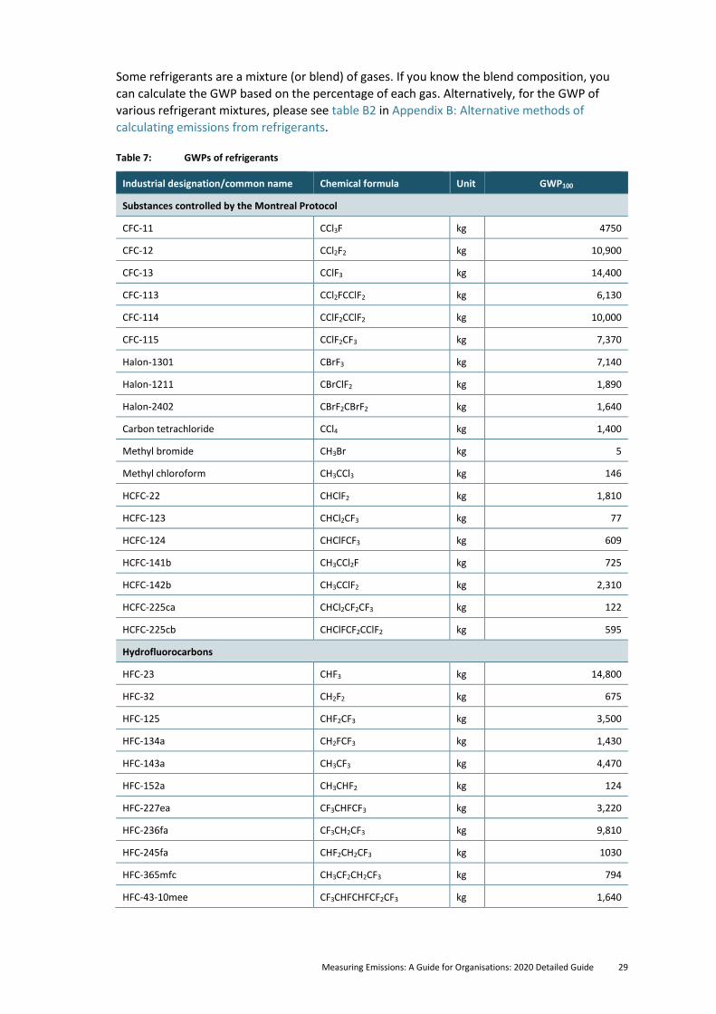
Some refrigerants are a mixture (or blend) of gases. If you know the blend composition, you
can calculate the GWP based on the percentage of each gas. Alternatively, for the GWP of
various refrigerant mixtures, please see table B2 in Appendix B: Alternative methods of
calculating emissions from refrigerants.
Table 7: GWPs of refrigerants
Industrial designation/common name Chemical formula Unit GWP100
Substances controlled by the Montreal Protocol
CFC-11 CCl3F kg 4750
CFC-12 CCl2F2 kg 10,900
CFC-13 CClF3 kg 14,400
CFC-113 CCl2FCClF2 kg 6,130
CFC-114 CClF2CClF2 kg 10,000
CFC-115 CClF2CF3 kg 7,370
Halon-1301 CBrF3 kg 7,140
Halon-1211 CBrClF2 kg 1,890
Halon-2402 CBrF2CBrF2 kg 1,640
Carbon tetrachloride CCl4 kg 1,400
Methyl bromide CH3Br kg 5
Methyl chloroform CH3CCl3 kg 146
HCFC-22 CHClF2 kg 1,810
HCFC-123 CHCl2CF3 kg 77
HCFC-124 CHClFCF3 kg 609
HCFC-141b CH3CCl2F kg 725
HCFC-142b CH3CClF2 kg 2,310
HCFC-225ca CHCl2CF2CF3 kg 122
HCFC-225cb CHClFCF2CClF2 kg 595
Hydrofluorocarbons
HFC-23 CHF3 kg 14,800
HFC-32 CH2F2 kg 675
HFC-125 CHF2CF3 kg 3,500
HFC-134a CH2FCF3 kg 1,430
HFC-143a CH3CF3 kg 4,470
HFC-152a CH3CHF2 kg 124
HFC-227ea CF3CHFCF3 kg 3,220
HFC-236fa CF3CH2CF3 kg 9,810
HFC-245fa CHF2CH2CF3 kg 1030
HFC-365mfc CH3CF2CH2CF3 kg 794
HFC-43-10mee CF3CHFCHFCF2CF3 kg 1,640
30 Measuring Emissions: A Guide for Organisations: 2020 Detailed Guide
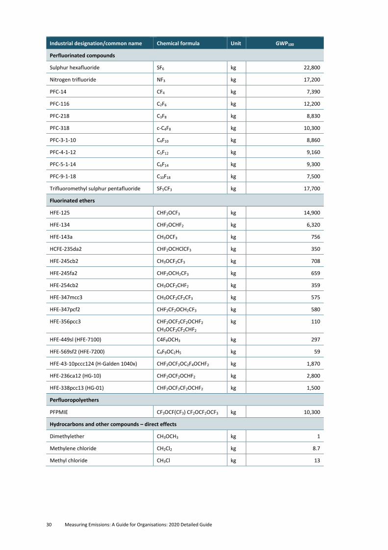
Industrial designation/common name Chemical formula Unit GWP100
Perfluorinated compounds
Sulphur hexafluoride SF6 kg 22,800
Nitrogen trifluoride NF3 kg 17,200
PFC-14 CF4 kg 7,390
PFC-116 C2F6 kg 12,200
PFC-218 C3F8 kg 8,830
PFC-318 c-C4F8 kg 10,300
PFC-3-1-10 C4F10 kg 8,860
PFC-4-1-12 C5F12 kg 9,160
PFC-5-1-14 C6F14 kg 9,300
PFC-9-1-18 C10F18 kg 7,500
Trifluoromethyl sulphur pentafluoride SF5CF3 kg 17,700
Fluorinated ethers
HFE-125 CHF2OCF3 kg 14,900
HFE-134 CHF2OCHF2 kg 6,320
HFE-143a CH3OCF3 kg 756
HCFE-235da2 CHF2OCHClCF3 kg 350
HFE-245cb2 CH3OCF2CF3 kg 708
HFE-245fa2 CHF2OCH2CF3 kg 659
HFE-254cb2 CH3OCF2CHF2 kg 359
HFE-347mcc3 CH3OCF2CF2CF3 kg 575
HFE-347pcf2 CHF2CF2OCH2CF3 kg 580
HFE-356pcc3 CHF2OCF2CF2OCHF2
CH3OCF2CF2CHF2
kg 110
HFE-449sl (HFE-7100) C4F9OCH3 kg 297
HFE-569sf2 (HFE-7200) C4F9OC2H5 kg 59
HFE-43-10pccc124 (H-Galden 1040x) CHF2OCF2OC2F4OCHF2 kg 1,870
HFE-236ca12 (HG-10) CHF2OCF2OCHF2 kg 2,800
HFE-338pcc13 (HG-01) CHF2OCF2CF2OCHF2 kg 1,500
Perfluoropolyethers
PFPMIE CF3OCF(CF3) CF2OCF2OCF3 kg 10,300
Hydrocarbons and other compounds – direct effects
Dimethylether CH3OCH3 kg 1
Methylene chloride CH2Cl2 kg 8.7
Methyl chloride CH3Cl kg 13
Measuring Emissions: A Guide for Organisations: 2020 Detailed Guide 31
4.2.2 GHG inventory development
There are three approaches to estimate HFC leakage from refrigeration equipment, depending
on the data available. The ideal method is the top-up method, Method A. Method B is the next
best option. Method C is the least preferred because it has the most assumptions.
It is stressed that for all methods, users must individually identify the type of refrigerant
because the GWPs vary widely.
Organisations should indicate the method(s) used in their inventories to reflect the levels of
accuracy and uncertainty.
4.2.3 Method A: Top-up
The best method to determine if emissions have occurred is through confirming if any top-ups
were necessary during the measurement period. A piece of equipment is ‘charged’ with
refrigerant gas, and any leaked gas must be replaced. Assuming that the system was full to
capacity before the leakage occurred and is full again after a top-up, the amount of top-up
gas is equal to the gas leaked or lost to the atmosphere. The equipment maintenance service
provider can typically provide information about the actual amount of refrigerant used to
replace what has leaked.
Gas used (kg) × GWP = Emissions (kg CO2-e)
Where:
• E = emissions from equipment in kg CO2-e
• GWP = the 100-year global warming potential of the refrigerant used in equipment (table 7).
4.2.4 Methods B and C: Screening
If top-up amounts are not available, we recommend using one of the following two methods
for estimating leakage, depending on the equipment and available information. Appendix B:
Alternative methods of calculating emissions from refrigerants details both methods.
Method B is based on default leakage rates and known refrigerant type and volume. Use Method
B when the type and amount of refrigerant held in a piece of equipment are known.
Method C is the same as Method B except that it allows default refrigerant quantities to be used
as well as default leakage rates. Use Method C to estimate both volume of refrigerant and
leakage rate when the amount of refrigerant held in a piece of equipment is not known.
Methods B and C are based on the screening approach outlined in the GHG Protocol HFC tool
(WRI/WBCSD, 2005).
For most equipment, Method B is acceptable, especially for factory and office situations where
refrigeration and air-conditioning equipment is incidental rather than central to operations.
In some cases, Method C is only suitable for a screening estimate. Screening is a way of
determining if the equipment should be included or excluded based on materiality of emissions
from refrigerants. Organisations should then try to source data based on the top-up method.
32 Measuring Emissions: A Guide for Organisations: 2020 Detailed Guide
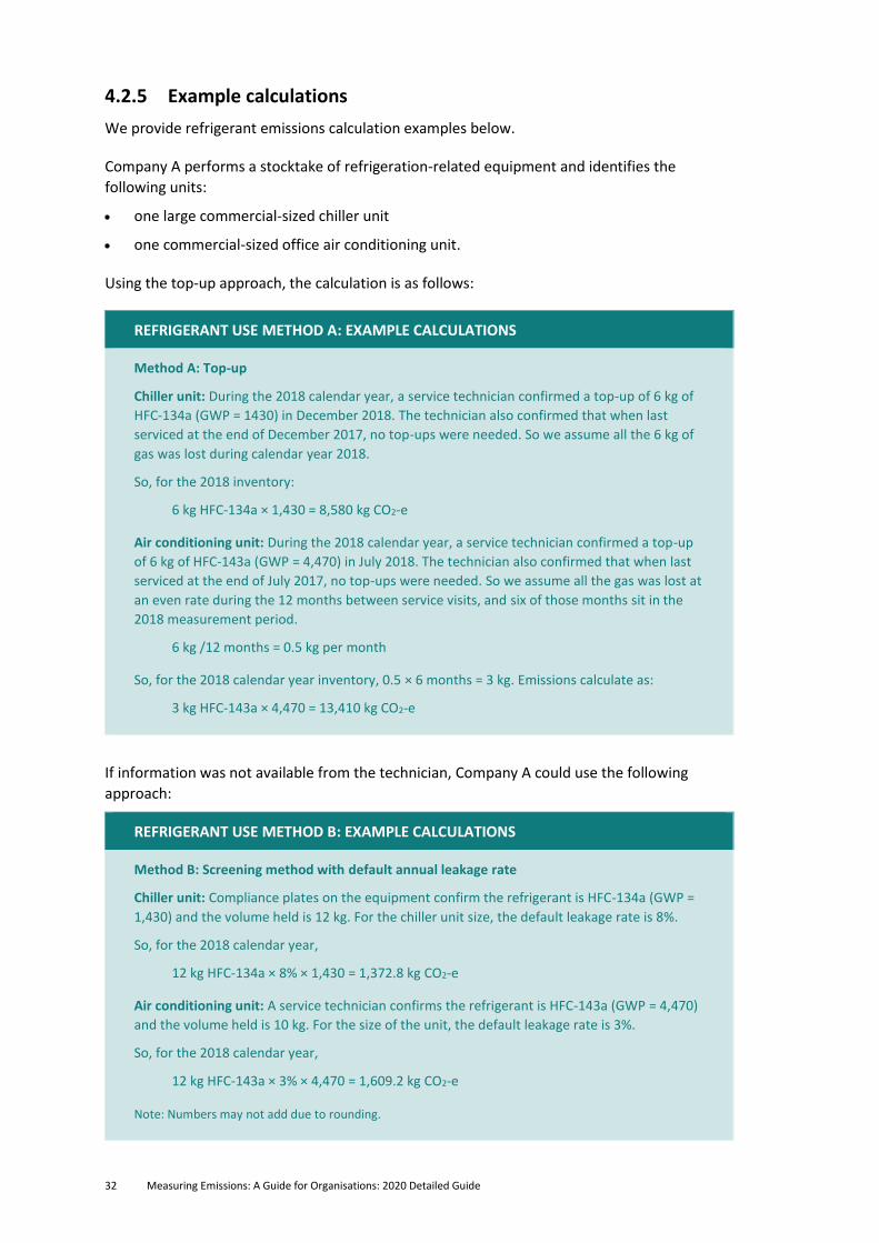
4.2.5 Example calculations
We provide refrigerant emissions calculation examples below.
Company A performs a stocktake of refrigeration-related equipment and identifies the
following units:
• one large commercial-sized chiller unit
• one commercial-sized office air conditioning unit.
Using the top-up approach, the calculation is as follows:
REFRIGERANT USE METHOD A: EXAMPLE CALCULATIONS
Method A: Top-up
Chiller unit: During the 2018 calendar year, a service technician confirmed a top-up of 6 kg of
HFC-134a (GWP = 1430) in December 2018. The technician also confirmed that when last
serviced at the end of December 2017, no top-ups were needed. So we assume all the 6 kg of
gas was lost during calendar year 2018.
So, for the 2018 inventory:
6 kg HFC-134a × 1,430 = 8,580 kg CO2-e
Air conditioning unit: During the 2018 calendar year, a service technician confirmed a top-up
of 6 kg of HFC-143a (GWP = 4,470) in July 2018. The technician also confirmed that when last
serviced at the end of July 2017, no top-ups were needed. So we assume all the gas was lost at
an even rate during the 12 months between service visits, and six of those months sit in the
2018 measurement period.
6 kg /12 months = 0.5 kg per month
So, for the 2018 calendar year inventory, 0.5 × 6 months = 3 kg. Emissions calculate as:
3 kg HFC-143a × 4,470 = 13,410 kg CO2-e
If information was not available from the technician, Company A could use the following
approach:
REFRIGERANT USE METHOD B: EXAMPLE CALCULATIONS
Method B: Screening method with default annual leakage rate
Chiller unit: Compliance plates on the equipment confirm the refrigerant is HFC-134a (GWP =
1,430) and the volume held is 12 kg. For the chiller unit size, the default leakage rate is 8%.
So, for the 2018 calendar year,
12 kg HFC-134a × 8% × 1,430 = 1,372.8 kg CO2-e
Air conditioning unit: A service technician confirms the refrigerant is HFC-143a (GWP = 4,470)
and the volume held is 10 kg. For the size of the unit, the default leakage rate is 3%.
So, for the 2018 calendar year,
12 kg HFC-143a × 3% × 4,470 = 1,609.2 kg CO2-e
Note: Numbers may not add due to rounding.
Measuring Emissions: A Guide for Organisations: 2020 Detailed Guide 33
The difference between Method A and Method B suggests that the leakage of refrigerant
exceeds the default leakage rate, so improved maintenance of the refrigeration systems
could help reduce leakage.
4.3 Medical gases use This section covers emissions from medical gases. Anaesthetic medical gases can be a
significant source of direct (Scope 1) emissions in hospitals. The most accurate way to
calculate emissions from medical gases is based on consumption data.
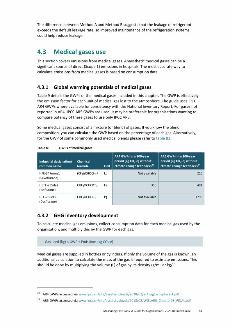
4.3.1 Global warming potentials of medical gases
Table 9 details the GWPs of the medical gases included in this chapter. The GWP is effectively
the emission factor for each unit of medical gas lost to the atmosphere. The guide uses IPCC
AR4 GWPs where available for consistency with the National Inventory Report. For gases not
reported in AR4, IPCC AR5 GWPs are used. It may be preferable for organisations wanting to
compare potency of these gases to use only IPCC AR5.
Some medical gases consist of a mixture (or blend) of gases. If you know the blend
composition, you can calculate the GWP based on the percentage of each gas. Alternatively,
for the GWP of some commonly used medical blends please refer to table B3.
Table 8: GWPs of medical gases
Industrial designation/
common name
Chemical
formula Unit
AR4 GWPs in a 100-year
period (kg CO2-e) without
climate change feedbacks23
AR5 GWPs in a 100-year
period (kg CO2-e) without
climate change feedbacks24
HFE-347mmz1
(Sevoflurane)
(CF3)2CHOCH2F kg Not available 216
HCFE-235da2
(Isoflurane)
CHF2OCHClCF3 kg 350 491
HFE-236ea2
(Desflurane)
CHF2OCHFCF3 kg Not available 1790
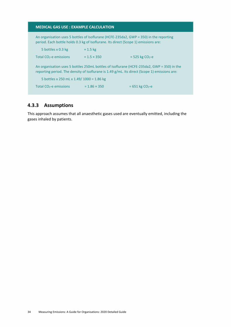
4.3.2 GHG inventory development
To calculate medical gas emissions, collect consumption data for each medical gas used by the
organisation, and multiply this by the GWP for each gas.
Gas used (kg) × GWP = Emissions (kg CO2-e)
Medical gases are supplied in bottles or cylinders. If only the volume of the gas is known, an
additional calculation to calculate the mass of the gas is required to estimate emissions. This
should be done by multiplying the volume (L) of gas by its density (g/mL or kg/L).
23 AR4 GWPs accessed via www.ipcc.ch/site/assets/uploads/2018/02/ar4-wg1-chapter2-1.pdf
24 AR5 GWPs accessed via www.ipcc.ch/site/assets/uploads/2018/02/WG1AR5_Chapter08_FINAL.pdf
34 Measuring Emissions: A Guide for Organisations: 2020 Detailed Guide
MEDICAL GAS USE : EXAMPLE CALCULATION
An organisation uses 5 bottles of Isoflurane (HCFE-235da2, GWP = 350) in the reporting
period. Each bottle holds 0.3 kg of Isoflurane. Its direct (Scope 1) emissions are:
5 bottles x 0.3 kg = 1.5 kg
Total CO2-e emissions = 1.5 × 350 = 525 kg CO2-e
An organisation uses 5 bottles 250mL bottles of Isoflurane (HCFE-235da2, GWP = 350) in the
reporting period. The density of Isoflurane is 1.49 g/mL. Its direct (Scope 1) emissions are:
5 bottles x 250 mL x 1.49/ 1000 = 1.86 kg
Total CO2-e emissions = 1.86 × 350 = 651 kg CO2-e
4.3.3 Assumptions
This approach assumes that all anaesthetic gases used are eventually emitted, including the
gases inhaled by patients.
Measuring Emissions: A Guide for Organisations: 2020 Detailed Guide 35
5 Purchased electricity, heat and steam emission factors
Purchased energy, in the form of electricity, heat or steam, is an indirect (Scope 2) emission.
This section also includes transmission and distribution losses for purchased electricity, which is
an indirect (Scope 3) emissions source.
Note that both the emission factor for purchased electricity and the emission factor for
transmission and distribution line losses align with the definitions in the GHG Protocol.
The guide provides information on reporting imported heat and steam and geothermal energy.
It does not provide emission factors for these categories as they are unique to a specific site.
5.1 Overview of changes since previous update In the eleventh version of the guide, we have included a time series of historic electricity
emission factors. This time series extends back to 2010, there is also an equivalent time series
for transmission and distribution losses.
There has been an update to the previous electricity emission factor as the data in the source
table has changed.
5.2 Direct emissions from purchased electricity from New Zealand grid
This guide applies to electricity purchased from a supplier that sources electricity from the
national grid (ie, purchased electricity consumed by end users). It does not cover on-site,
self-generated electricity.
The grid-average emission factor best reflects the carbon dioxide equivalent emissions
associated with the generation of a unit of electricity purchased from the national grid in
New Zealand in 2020. We recommend the use of the emissions factors in table 9 for all
electricity purchased from the national grid.
We calculate purchased electricity emission factors on a calendar-year basis, and based on the
average grid mix of generation types for the 2018 year. The emission factor accounts for the
emissions from fuel combustion at thermal power stations and fugitive emissions from the
generation of geothermal electricity. Thermal electricity is generated by burning fossil fuels.
The emission factor for purchased grid-average electricity does not include transmission and
distribution losses. We provide a separate average emission factor for this as an indirect
(Scope 3) emission source in section 5.3.
This emission factor also doesn’t reflect the real-world factors that influence the carbon
intensity of the grid such as time of year, time of day and geographical area. Therefore, a
grid-average emission factor may over- or underestimate your organisation’s GHG emissions.
Detailed additional guidance on reporting electricity emissions is available in the GHG Protocol
Scope 2 Guidance.
36 Measuring Emissions: A Guide for Organisations: 2020 Detailed Guide
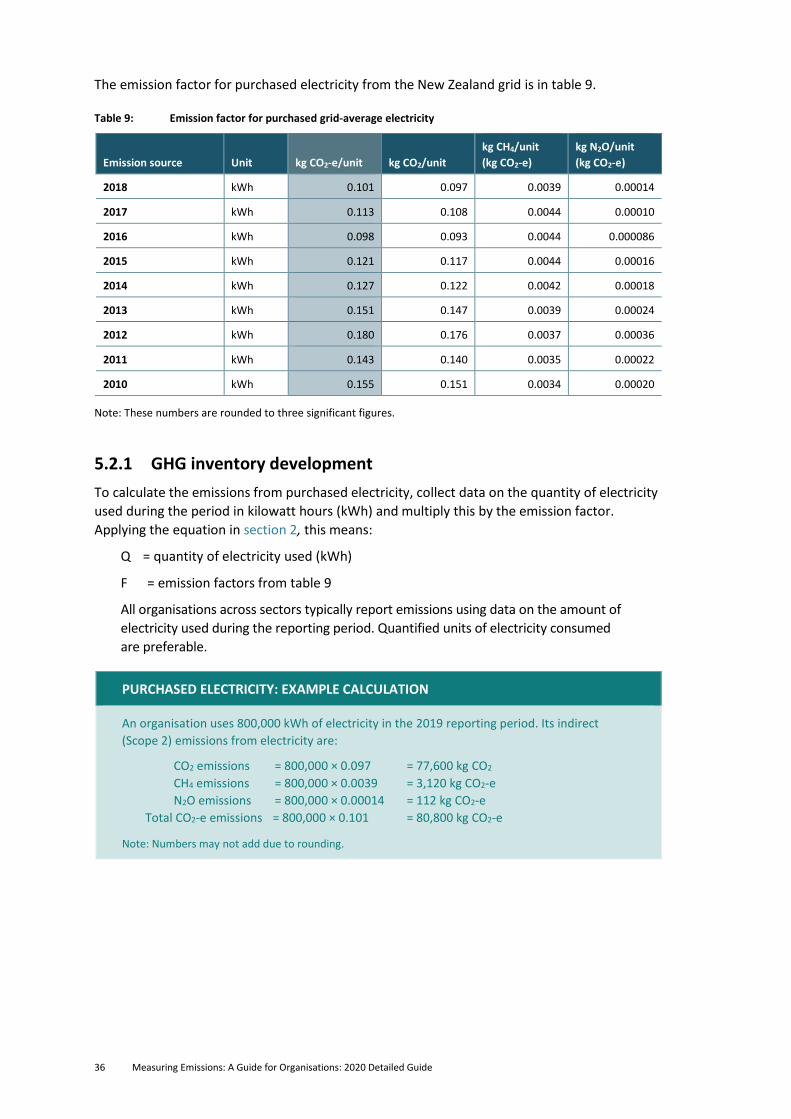
The emission factor for purchased electricity from the New Zealand grid is in table 9.
Table 9: Emission factor for purchased grid-average electricity
Emission source Unit kg CO2-e/unit kg CO2/unit
kg CH4/unit
(kg CO2-e)
kg N2O/unit
(kg CO2-e)
2018 kWh 0.101 0.097 0.0039 0.00014
2017 kWh 0.113 0.108 0.0044 0.00010
2016 kWh 0.098 0.093 0.0044 0.000086
2015 kWh 0.121 0.117 0.0044 0.00016
2014 kWh 0.127 0.122 0.0042 0.00018
2013 kWh 0.151 0.147 0.0039 0.00024
2012 kWh 0.180 0.176 0.0037 0.00036
2011 kWh 0.143 0.140 0.0035 0.00022
2010 kWh 0.155 0.151 0.0034 0.00020
Note: These numbers are rounded to three significant figures.
5.2.1 GHG inventory development
To calculate the emissions from purchased electricity, collect data on the quantity of electricity
used during the period in kilowatt hours (kWh) and multiply this by the emission factor.
Applying the equation in section 2, this means:
Q = quantity of electricity used (kWh)
F = emission factors from table 9
All organisations across sectors typically report emissions using data on the amount of
electricity used during the reporting period. Quantified units of electricity consumed
are preferable.
PURCHASED ELECTRICITY: EXAMPLE CALCULATION
An organisation uses 800,000 kWh of electricity in the 2019 reporting period. Its indirect
(Scope 2) emissions from electricity are:
CO2 emissions = 800,000 × 0.097 = 77,600 kg CO2
CH4 emissions = 800,000 × 0.0039 = 3,120 kg CO2-e
N2O emissions = 800,000 × 0.00014 = 112 kg CO2-e
Total CO2-e emissions = 800,000 × 0.101 = 80,800 kg CO2-e
Note: Numbers may not add due to rounding.
Measuring Emissions: A Guide for Organisations: 2020 Detailed Guide 37
5.2.2 Emission factor derivation methodology
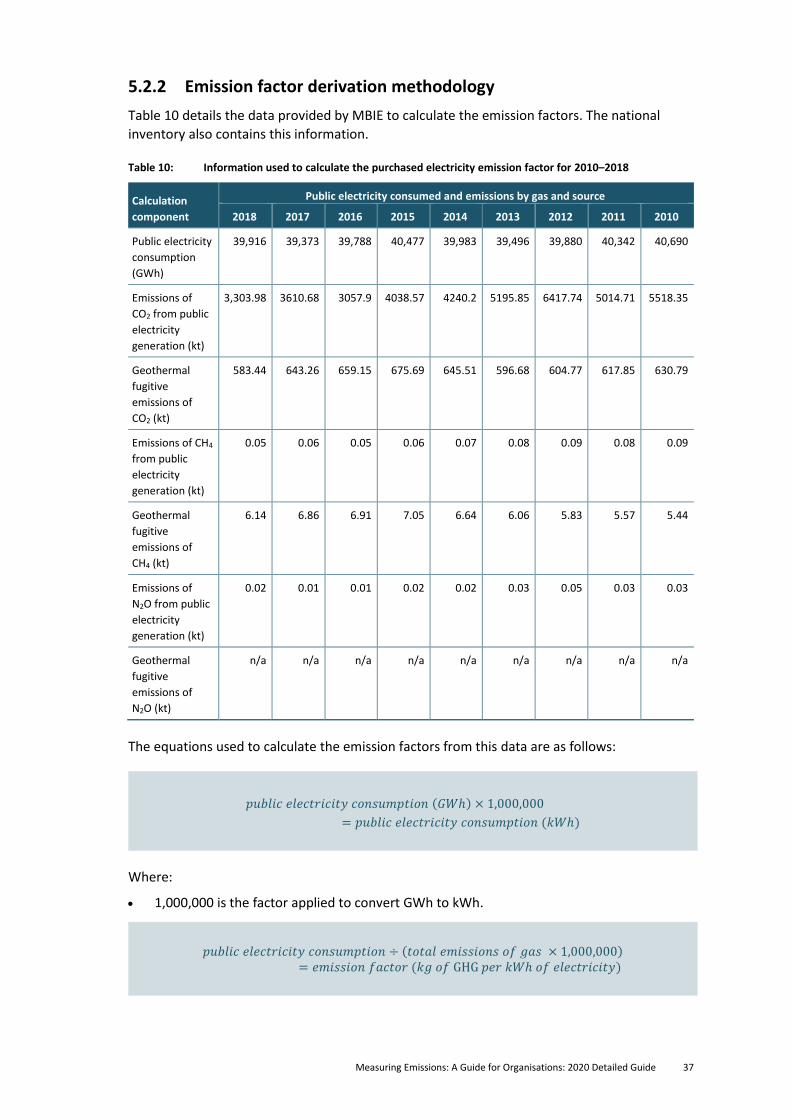
Table 10 details the data provided by MBIE to calculate the emission factors. The national
inventory also contains this information.
Table 10: Information used to calculate the purchased electricity emission factor for 2010–2018
Calculation
component
Public electricity consumed and emissions by gas and source
2018 2017 2016 2015 2014 2013 2012 2011 2010
Public electricity
consumption
(GWh)
39,916 39,373 39,788 40,477 39,983 39,496 39,880 40,342 40,690
Emissions of
CO2 from public
electricity
generation (kt)
3,303.98 3610.68 3057.9 4038.57 4240.2 5195.85 6417.74 5014.71 5518.35
Geothermal
fugitive
emissions of
CO2 (kt)
583.44 643.26 659.15 675.69 645.51 596.68 604.77 617.85 630.79
Emissions of CH4
from public
electricity
generation (kt)
0.05 0.06 0.05 0.06 0.07 0.08 0.09 0.08 0.09
Geothermal
fugitive
emissions of
CH4 (kt)
6.14 6.86 6.91 7.05 6.64 6.06 5.83 5.57 5.44
Emissions of
N2O from public
electricity
generation (kt)
0.02 0.01 0.01 0.02 0.02 0.03 0.05 0.03 0.03
Geothermal
fugitive
emissions of
N2O (kt)
n/a n/a n/a n/a n/a n/a n/a n/a n/a
The equations used to calculate the emission factors from this data are as follows:
𝑝𝑢𝑏𝑙𝑖𝑐 𝑒𝑙𝑒𝑐𝑡𝑟𝑖𝑐𝑖𝑡𝑦 𝑐𝑜𝑛𝑠𝑢𝑚𝑝𝑡𝑖𝑜𝑛 (𝐺𝑊ℎ) × 1,000,000
= 𝑝𝑢𝑏𝑙𝑖𝑐 𝑒𝑙𝑒𝑐𝑡𝑟𝑖𝑐𝑖𝑡𝑦 𝑐𝑜𝑛𝑠𝑢𝑚𝑝𝑡𝑖𝑜𝑛 (𝑘𝑊ℎ)
Where:
• 1,000,000 is the factor applied to convert GWh to kWh.
𝑝𝑢𝑏𝑙𝑖𝑐 𝑒𝑙𝑒𝑐𝑡𝑟𝑖𝑐𝑖𝑡𝑦 𝑐𝑜𝑛𝑠𝑢𝑚𝑝𝑡𝑖𝑜𝑛 ÷ (𝑡𝑜𝑡𝑎𝑙 𝑒𝑚𝑖𝑠𝑠𝑖𝑜𝑛𝑠 𝑜𝑓 𝑔𝑎𝑠 × 1,000,000)= 𝑒𝑚𝑖𝑠𝑠𝑖𝑜𝑛 𝑓𝑎𝑐𝑡𝑜𝑟 (𝑘𝑔 𝑜𝑓 GHG 𝑝𝑒𝑟 𝑘𝑊ℎ 𝑜𝑓 𝑒𝑙𝑒𝑐𝑡𝑟𝑖𝑐𝑖𝑡𝑦)
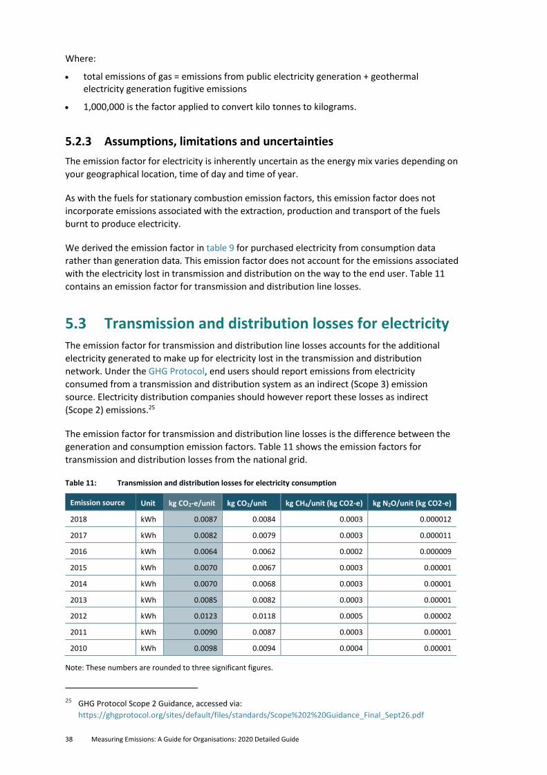
38 Measuring Emissions: A Guide for Organisations: 2020 Detailed Guide
Where:
• total emissions of gas = emissions from public electricity generation + geothermal electricity generation fugitive emissions
• 1,000,000 is the factor applied to convert kilo tonnes to kilograms.
5.2.3 Assumptions, limitations and uncertainties
The emission factor for electricity is inherently uncertain as the energy mix varies depending on
your geographical location, time of day and time of year.
As with the fuels for stationary combustion emission factors, this emission factor does not
incorporate emissions associated with the extraction, production and transport of the fuels
burnt to produce electricity.
We derived the emission factor in table 9 for purchased electricity from consumption data
rather than generation data. This emission factor does not account for the emissions associated
with the electricity lost in transmission and distribution on the way to the end user. Table 11
contains an emission factor for transmission and distribution line losses.
5.3 Transmission and distribution losses for electricity The emission factor for transmission and distribution line losses accounts for the additional
electricity generated to make up for electricity lost in the transmission and distribution
network. Under the GHG Protocol, end users should report emissions from electricity
consumed from a transmission and distribution system as an indirect (Scope 3) emission
source. Electricity distribution companies should however report these losses as indirect
(Scope 2) emissions.25
The emission factor for transmission and distribution line losses is the difference between the
generation and consumption emission factors. Table 11 shows the emission factors for
transmission and distribution losses from the national grid.
Table 11: Transmission and distribution losses for electricity consumption
Emission source Unit kg CO2-e/unit kg CO2/unit kg CH4/unit (kg CO2-e) kg N2O/unit (kg CO2-e)
2018 kWh 0.0087 0.0084 0.0003 0.000012
2017 kWh 0.0082 0.0079 0.0003 0.000011
2016 kWh 0.0064 0.0062 0.0002 0.000009
2015 kWh 0.0070 0.0067 0.0003 0.00001
2014 kWh 0.0070 0.0068 0.0003 0.00001
2013 kWh 0.0085 0.0082 0.0003 0.00001
2012 kWh 0.0123 0.0118 0.0005 0.00002
2011 kWh 0.0090 0.0087 0.0003 0.00001
2010 kWh 0.0098 0.0094 0.0004 0.00001
Note: These numbers are rounded to three significant figures.
25 GHG Protocol Scope 2 Guidance, accessed via:
https://ghgprotocol.org/sites/default/files/standards/Scope%202%20Guidance_Final_Sept26.pdf
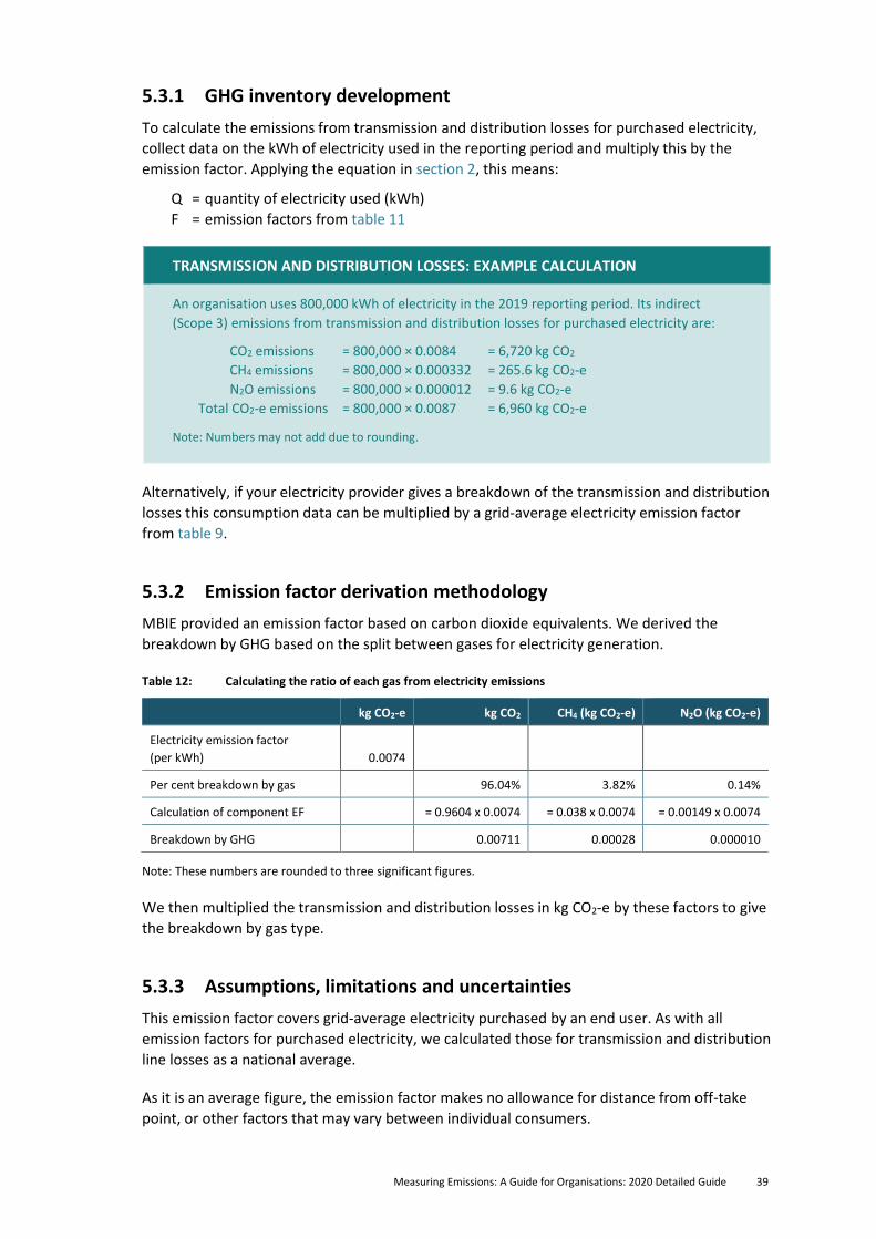
Measuring Emissions: A Guide for Organisations: 2020 Detailed Guide 39
5.3.1 GHG inventory development
To calculate the emissions from transmission and distribution losses for purchased electricity,
collect data on the kWh of electricity used in the reporting period and multiply this by the
emission factor. Applying the equation in section 2, this means:
Q = quantity of electricity used (kWh)
F = emission factors from table 11
TRANSMISSION AND DISTRIBUTION LOSSES: EXAMPLE CALCULATION
An organisation uses 800,000 kWh of electricity in the 2019 reporting period. Its indirect
(Scope 3) emissions from transmission and distribution losses for purchased electricity are:
CO2 emissions = 800,000 × 0.0084 = 6,720 kg CO2
CH4 emissions = 800,000 × 0.000332 = 265.6 kg CO2-e
N2O emissions = 800,000 × 0.000012 = 9.6 kg CO2-e
Total CO2-e emissions = 800,000 × 0.0087 = 6,960 kg CO2-e
Note: Numbers may not add due to rounding.
Alternatively, if your electricity provider gives a breakdown of the transmission and distribution
losses this consumption data can be multiplied by a grid-average electricity emission factor
from table 9.
5.3.2 Emission factor derivation methodology
MBIE provided an emission factor based on carbon dioxide equivalents. We derived the
breakdown by GHG based on the split between gases for electricity generation.
Table 12: Calculating the ratio of each gas from electricity emissions
kg CO2-e kg CO2 CH4 (kg CO2-e) N2O (kg CO2-e)
Electricity emission factor
(per kWh) 0.0074
Per cent breakdown by gas 96.04% 3.82% 0.14%
Calculation of component EF = 0.9604 x 0.0074 = 0.038 x 0.0074 = 0.00149 x 0.0074
Breakdown by GHG 0.00711 0.00028 0.000010
Note: These numbers are rounded to three significant figures.
We then multiplied the transmission and distribution losses in kg CO2-e by these factors to give
the breakdown by gas type.
5.3.3 Assumptions, limitations and uncertainties
This emission factor covers grid-average electricity purchased by an end user. As with all
emission factors for purchased electricity, we calculated those for transmission and distribution
line losses as a national average.
As it is an average figure, the emission factor makes no allowance for distance from off-take
point, or other factors that may vary between individual consumers.
40 Measuring Emissions: A Guide for Organisations: 2020 Detailed Guide
This emission factor does not incorporate the emissions associated with the extraction,
production and transport of the fuels burnt to produce the electricity.
5.4 Imported heat and steam Organisations that have a specific heat or steam external energy source (such as a district
heating scheme) can calculate emissions using an emission factor specific to that scheme.
This should be available from the owner of the external energy source.
5.5 Geothermal energy Organisations that have their own geothermal energy source can calculate emissions separately
using a unique emission factor. Depending on the steam coming from the borehole, there may
or may not be emissions associated with this energy type.
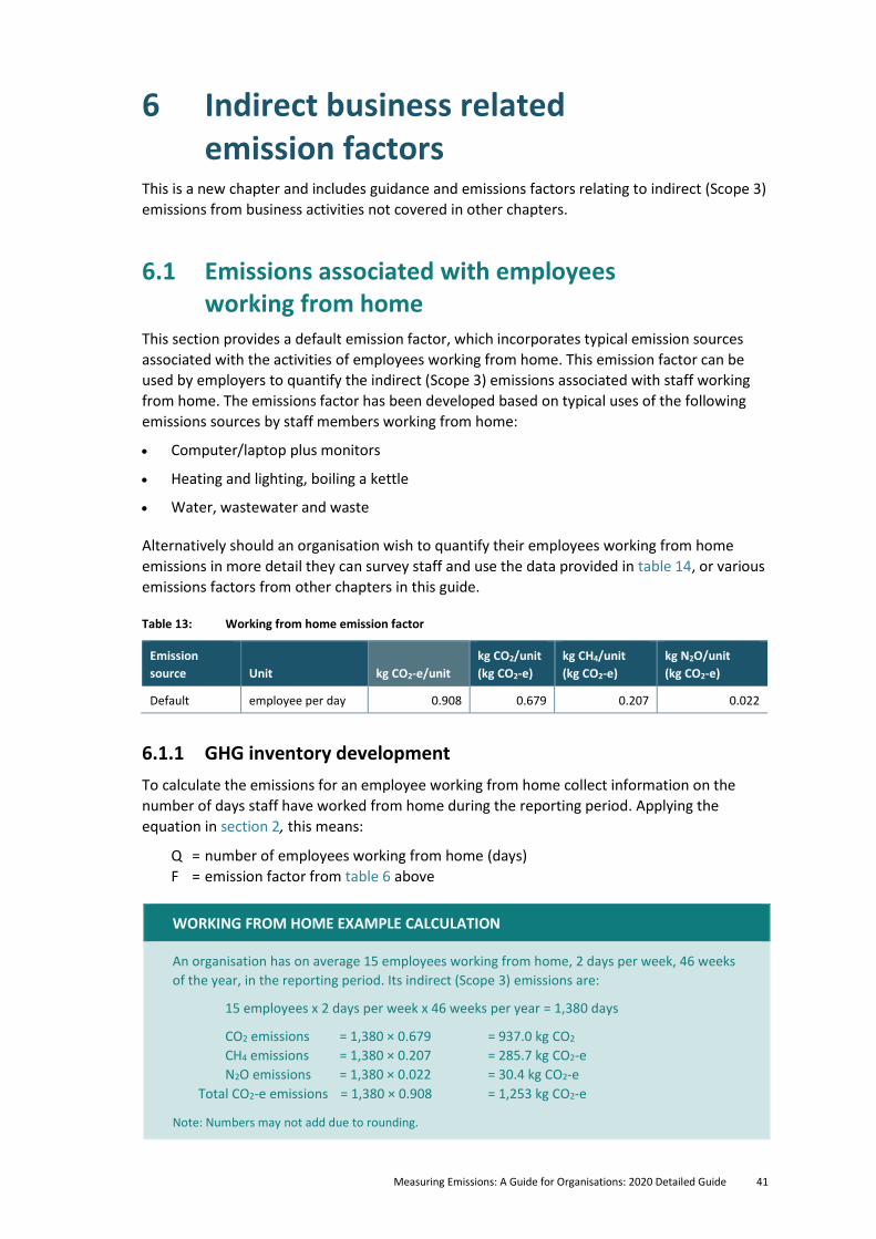
Measuring Emissions: A Guide for Organisations: 2020 Detailed Guide 41
6 Indirect business related emission factors
This is a new chapter and includes guidance and emissions factors relating to indirect (Scope 3)
emissions from business activities not covered in other chapters.
6.1 Emissions associated with employees working from home
This section provides a default emission factor, which incorporates typical emission sources
associated with the activities of employees working from home. This emission factor can be
used by employers to quantify the indirect (Scope 3) emissions associated with staff working
from home. The emissions factor has been developed based on typical uses of the following
emissions sources by staff members working from home:
• Computer/laptop plus monitors
• Heating and lighting, boiling a kettle
• Water, wastewater and waste
Alternatively should an organisation wish to quantify their employees working from home
emissions in more detail they can survey staff and use the data provided in table 14, or various
emissions factors from other chapters in this guide.
Table 13: Working from home emission factor
Emission
source Unit kg CO2-e/unit
kg CO2/unit
(kg CO2-e)
kg CH4/unit
(kg CO2-e)
kg N2O/unit
(kg CO2-e)
Default employee per day 0.908 0.679 0.207 0.022
6.1.1 GHG inventory development
To calculate the emissions for an employee working from home collect information on the
number of days staff have worked from home during the reporting period. Applying the
equation in section 2, this means:
Q = number of employees working from home (days)
F = emission factor from table 6 above
WORKING FROM HOME EXAMPLE CALCULATION
An organisation has on average 15 employees working from home, 2 days per week, 46 weeks
of the year, in the reporting period. Its indirect (Scope 3) emissions are:
15 employees x 2 days per week x 46 weeks per year = 1,380 days
CO2 emissions = 1,380 × 0.679 = 937.0 kg CO2
CH4 emissions = 1,380 × 0.207 = 285.7 kg CO2-e
N2O emissions = 1,380 × 0.022 = 30.4 kg CO2-e
Total CO2-e emissions = 1,380 × 0.908 = 1,253 kg CO2-e
Note: Numbers may not add due to rounding.
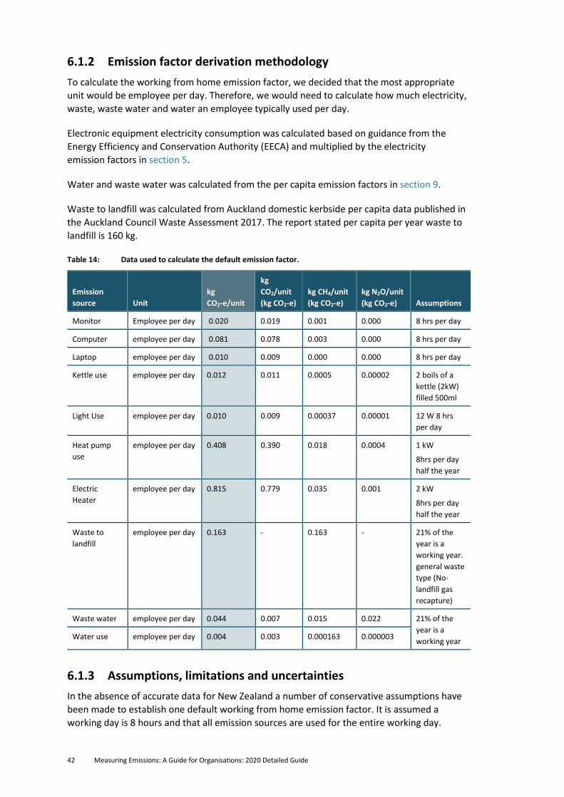
42 Measuring Emissions: A Guide for Organisations: 2020 Detailed Guide
6.1.2 Emission factor derivation methodology
To calculate the working from home emission factor, we decided that the most appropriate
unit would be employee per day. Therefore, we would need to calculate how much electricity,
waste, waste water and water an employee typically used per day.
Electronic equipment electricity consumption was calculated based on guidance from the
Energy Efficiency and Conservation Authority (EECA) and multiplied by the electricity
emission factors in section 5.
Water and waste water was calculated from the per capita emission factors in section 9.
Waste to landfill was calculated from Auckland domestic kerbside per capita data published in
the Auckland Council Waste Assessment 2017. The report stated per capita per year waste to
landfill is 160 kg.
Table 14: Data used to calculate the default emission factor.
Emission
source Unit
kg
CO2-e/unit
kg
CO2/unit
(kg CO2-e)
kg CH4/unit
(kg CO2-e)
kg N2O/unit
(kg CO2-e) Assumptions
Monitor Employee per day 0.020 0.019 0.001 0.000 8 hrs per day
Computer employee per day 0.081 0.078 0.003 0.000 8 hrs per day
Laptop employee per day 0.010 0.009 0.000 0.000 8 hrs per day
Kettle use employee per day 0.012 0.011 0.0005 0.00002 2 boils of a
kettle (2kW)
filled 500ml
Light Use employee per day 0.010 0.009 0.00037 0.00001 12 W 8 hrs
per day
Heat pump
use
employee per day 0.408 0.390 0.018 0.0004 1 kW
8hrs per day
half the year
Electric
Heater
employee per day 0.815 0.779 0.035 0.001 2 kW
8hrs per day
half the year
Waste to
landfill
employee per day 0.163 - 0.163 - 21% of the
year is a
working year.
general waste
type (No-
landfill gas
recapture)
Waste water employee per day 0.044 0.007 0.015 0.022 21% of the
year is a
working year Water use employee per day 0.004 0.003 0.000163 0.000003
6.1.3 Assumptions, limitations and uncertainties
In the absence of accurate data for New Zealand a number of conservative assumptions have
been made to establish one default working from home emission factor. It is assumed a
working day is 8 hours and that all emission sources are used for the entire working day.
Measuring Emissions: A Guide for Organisations: 2020 Detailed Guide 43
Heating, the biggest contributor to the emission factor, is assumed to be used half of the
year. In addition it is assumed that fifty percent of staff use heaters while fifty percent use
heat pumps. Likewise fifty percent of staff use desktops and fifty percent of staff use laptops.
It is assumed all staff use a monitor, a 12W LED light, and boil two cups (500 mL) of water
twice per day.
Based on working hours of 40 hours per week and 46 weeks of the year, waste water and
water use are assumed to be 21 per cent of the per capita emission factor for waste water
and water use. Furthermore, waste to landfill volume is assumed to be 21 per cent of Auckland
domestic kerbside refuse per capita per year as general waste disposed in a landfill without
gas recapture.
6.2 Guidance on the use of cloud-based data centres Emissions from data centres come under indirect (Scope 3) emissions. These emissions may
be significant for any organization that operates with large third party IT infrastructure.
Due to the diversity and country location of data centres utilized by organisations in
New Zealand it is not possible to produce a single emission factor that would inform users
of the kg CO2-e each gigabyte of data produces.
Therefore, organisations seeking to find out what the footprint is of the data centres where
their “cloud” is stored should contact the providers of their data centre to request this
information. Data centre providers such as Google, Microsoft and Amazon may be calculating
the total emissions from their data centres and therefore be able to inform users of the carbon
footprint of their usage.
44 Measuring Emissions: A Guide for Organisations: 2020 Detailed Guide
7 Travel emission factors
Travel emissions result from travel associated with (and generally paid for by) the
organisation. We provide factors for private and rental vehicles, taxis, public transport,
air travel and accommodation.
Travel emissions are indirect (Scope 3) if the organisation does not directly own or control
the vehicles used for travel. If the organisation owns or has an operating lease for the
vehicle(s) these emissions are direct (Scope 1) and should be accounted for in transport
fuels (see section 3.3).
Travel emission factors are in line with ISO 14064-1:2018 and the GHG Protocol. We also
include the methodology of the corresponding emission factors.
7.1 Overview of changes since previous update There has been one major change to travel emission factors since the previous version, which is
the introduction of public transport passenger emissions factors for passenger travel on bus
and rail. No data is currently available for ferries.
7.2 Passenger vehicles This section covers emissions from private vehicles for which mileage is claimed, rental vehicles
and taxi travel.
Travel in rental vehicles is a common source of direct (Scope 1) emissions for many
organisations, while staff mileage and taxi travel are indirect (Scope 3) emissions. As with
direct (Scope 1) emissions from transport fuels, the most accurate way to calculate emissions
is based on fuel consumption data. Fuel-use data are preferable because factors such as
individual vehicle fuel efficiency and driving efficiency mean that kilometre-based estimates
of emissions are less accurate. However, this information may not be easily available.
Fuel-use based emission factors are above in section 3.
If you only have information on kilometres travelled, use the emission factors in this section.
Factors such as individual vehicle fuel efficiency and driving efficiency mean that kilometre-
based estimates of carbon dioxide equivalent emissions are less accurate than calculating
emissions based on fuel-use data.
If the vehicle size and engine type are known, use the factors in table 16 to table 18. Table 19
lists default private car emission factors, and table 20 lists the rental car emission factors based
on distance travelled. Table 21 lists emission factors for taxi travel based on dollars spent and
kilometres travelled.
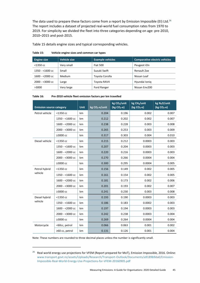
Measuring Emissions: A Guide for Organisations: 2020 Detailed Guide 45
The data used to prepare these factors come from a report by Emission Impossible (EI) Ltd.26
The report includes a dataset of projected real-world fuel consumption rates from 1970 to
2019. For simplicity we divided the fleet into three categories depending on age: pre-2010,
2010–2015 and post-2015.
Table 15 details engine sizes and typical corresponding vehicles.
Table 15: Vehicle engine sizes and common car types
Engine size Vehicle size Example vehicles Comparative electric vehicles
<1350 cc Very small Fiat 500 Peugeot iOn
1350 - <1600 cc Small Suzuki Swift Renault Zoe
1600 - <2000 cc Medium Toyota Corolla Nissan Leaf
2000 - <3000 cc Large Toyota RAV4 Hyundai Ioniq
>3000 Very large Ford Ranger Nissan Env200
Table 16: Pre-2010 vehicle fleet emission factors per km travelled
Emission source category Unit kg CO2-e/unit
kg CO2/unit
(kg CO2-e)
kg CH4/unit
(kg CO2-e)
kg N2O/unit
(kg CO2-e)
Petrol vehicle <1350 cc km 0.204 0.196 0.002 0.007
1350 - <1600 cc km 0.212 0.202 0.002 0.007
1600 - <2000 cc km 0.238 0.228 0.003 0.008
2000 - <3000 cc km 0.265 0.253 0.003 0.009
≥3000 cc km 0.317 0.303 0.004 0.010
Diesel vehicle <1350 cc km 0.215 0.212 0.0003 0.003
1350 - <1600 cc km 0.207 0.204 0.0003 0.003
1600 - <2000 cc km 0.220 0.216 0.0003 0.003
2000 - <3000 cc km 0.270 0.266 0.0004 0.004
≥3000 cc km 0.300 0.295 0.0004 0.005
Petrol hybrid
vehicle
<1350 cc km 0.156 0.149 0.002 0.005
1350 - <1600 cc km 0.161 0.154 0.002 0.005
1600 - <2000 cc km 0.181 0.173 0.002 0.006
2000 - <3000 cc km 0.201 0.193 0.002 0.007
≥3000 cc km 0.241 0.230 0.003 0.008
Diesel hybrid
vehicle
<1350 cc km 0.193 0.190 0.0003 0.003
1350 - <1600 cc km 0.186 0.183 0.0002 0.003
1600 - <2000 cc km 0.197 0.194 0.0003 0.003
2000 - <3000 cc km 0.242 0.238 0.0003 0.004
≥3000 cc km 0.269 0.264 0.0004 0.004
Motorcycle <60cc, petrol km 0.066 0.063 0.001 0.002
≥60 cc, petrol km 0.131 0.126 0.001 0.004
Note: These numbers are rounded to three decimal places unless the number is significantly small.
26 Real world energy use projections for VFEM (Report prepared for MoT), Emission Impossible, 2016. Online:
www.transport.govt.nz/assets/Uploads/Research/Transport-Outlook/Documents/a9189b9da0/Emission-
Impossible-Real-World-Energy-Use-Projections-for-VFEM-20160905.pdf
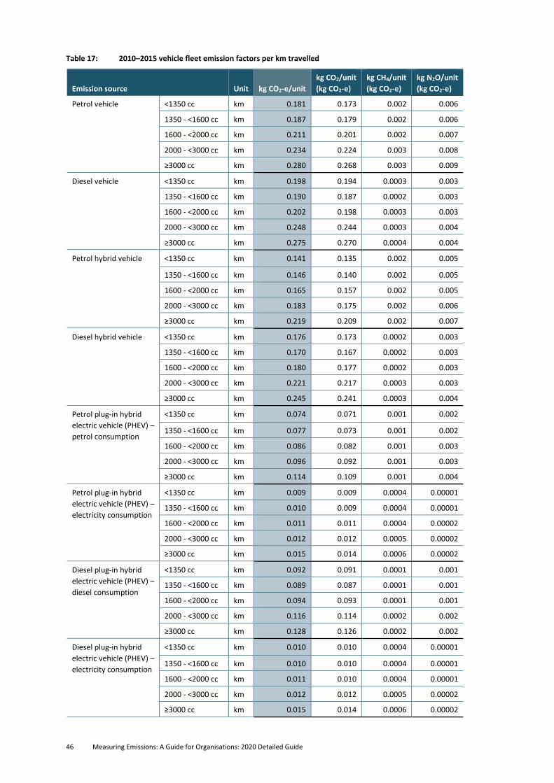
46 Measuring Emissions: A Guide for Organisations: 2020 Detailed Guide
Table 17: 2010–2015 vehicle fleet emission factors per km travelled
Emission source Unit kg CO2-e/unit
kg CO2/unit
(kg CO2-e)
kg CH4/unit
(kg CO2-e)
kg N2O/unit
(kg CO2-e)
Petrol vehicle <1350 cc km 0.181 0.173 0.002 0.006
1350 - <1600 cc km 0.187 0.179 0.002 0.006
1600 - <2000 cc km 0.211 0.201 0.002 0.007
2000 - <3000 cc km 0.234 0.224 0.003 0.008
≥3000 cc km 0.280 0.268 0.003 0.009
Diesel vehicle <1350 cc km 0.198 0.194 0.0003 0.003
1350 - <1600 cc km 0.190 0.187 0.0002 0.003
1600 - <2000 cc km 0.202 0.198 0.0003 0.003
2000 - <3000 cc km 0.248 0.244 0.0003 0.004
≥3000 cc km 0.275 0.270 0.0004 0.004
Petrol hybrid vehicle <1350 cc km 0.141 0.135 0.002 0.005
1350 - <1600 cc km 0.146 0.140 0.002 0.005
1600 - <2000 cc km 0.165 0.157 0.002 0.005
2000 - <3000 cc km 0.183 0.175 0.002 0.006
≥3000 cc km 0.219 0.209 0.002 0.007
Diesel hybrid vehicle <1350 cc km 0.176 0.173 0.0002 0.003
1350 - <1600 cc km 0.170 0.167 0.0002 0.003
1600 - <2000 cc km 0.180 0.177 0.0002 0.003
2000 - <3000 cc km 0.221 0.217 0.0003 0.003
≥3000 cc km 0.245 0.241 0.0003 0.004
Petrol plug-in hybrid
electric vehicle (PHEV) –
petrol consumption
<1350 cc km 0.074 0.071 0.001 0.002
1350 - <1600 cc km 0.077 0.073 0.001 0.002
1600 - <2000 cc km 0.086 0.082 0.001 0.003
2000 - <3000 cc km 0.096 0.092 0.001 0.003
≥3000 cc km 0.114 0.109 0.001 0.004
Petrol plug-in hybrid
electric vehicle (PHEV) –
electricity consumption
<1350 cc km 0.009 0.009 0.0004 0.00001
1350 - <1600 cc km 0.010 0.009 0.0004 0.00001
1600 - <2000 cc km 0.011 0.011 0.0004 0.00002
2000 - <3000 cc km 0.012 0.012 0.0005 0.00002
≥3000 cc km 0.015 0.014 0.0006 0.00002
Diesel plug-in hybrid
electric vehicle (PHEV) –
diesel consumption
<1350 cc km 0.092 0.091 0.0001 0.001
1350 - <1600 cc km 0.089 0.087 0.0001 0.001
1600 - <2000 cc km 0.094 0.093 0.0001 0.001
2000 - <3000 cc km 0.116 0.114 0.0002 0.002
≥3000 cc km 0.128 0.126 0.0002 0.002
Diesel plug-in hybrid
electric vehicle (PHEV) –
electricity consumption
<1350 cc km 0.010 0.010 0.0004 0.00001
1350 - <1600 cc km 0.010 0.010 0.0004 0.00001
1600 - <2000 cc km 0.011 0.010 0.0004 0.00001
2000 - <3000 cc km 0.012 0.012 0.0005 0.00002
≥3000 cc km 0.015 0.014 0.0006 0.00002
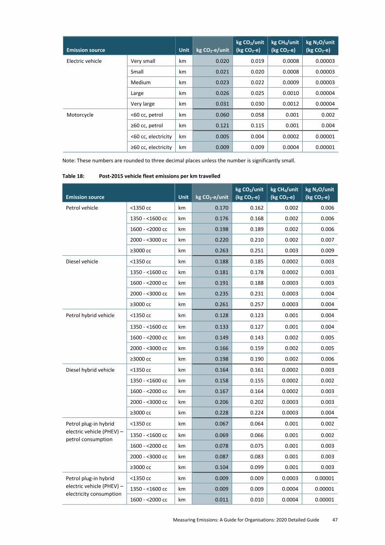
Measuring Emissions: A Guide for Organisations: 2020 Detailed Guide 47
Emission source Unit kg CO2-e/unit
kg CO2/unit
(kg CO2-e)
kg CH4/unit
(kg CO2-e)
kg N2O/unit
(kg CO2-e)
Electric vehicle Very small km 0.020 0.019 0.0008 0.00003
Small km 0.021 0.020 0.0008 0.00003
Medium km 0.023 0.022 0.0009 0.00003
Large km 0.026 0.025 0.0010 0.00004
Very large km 0.031 0.030 0.0012 0.00004
Motorcycle <60 cc, petrol km 0.060 0.058 0.001 0.002
≥60 cc, petrol km 0.121 0.115 0.001 0.004
<60 cc, electricity km 0.005 0.004 0.0002 0.00001
≥60 cc, electricity km 0.009 0.009 0.0004 0.00001
Note: These numbers are rounded to three decimal places unless the number is significantly small.
Table 18: Post-2015 vehicle fleet emissions per km travelled
Emission source Unit kg CO2-e/unit
kg CO2/unit
(kg CO2-e)
kg CH4/unit
(kg CO2-e)
kg N2O/unit
(kg CO2-e)
Petrol vehicle <1350 cc km 0.170 0.162 0.002 0.006
1350 - <1600 cc km 0.176 0.168 0.002 0.006
1600 - <2000 cc km 0.198 0.189 0.002 0.006
2000 - <3000 cc km 0.220 0.210 0.002 0.007
≥3000 cc km 0.263 0.251 0.003 0.009
Diesel vehicle <1350 cc km 0.188 0.185 0.0002 0.003
1350 - <1600 cc km 0.181 0.178 0.0002 0.003
1600 - <2000 cc km 0.191 0.188 0.0003 0.003
2000 - <3000 cc km 0.235 0.231 0.0003 0.004
≥3000 cc km 0.261 0.257 0.0003 0.004
Petrol hybrid vehicle <1350 cc km 0.128 0.123 0.001 0.004
1350 - <1600 cc km 0.133 0.127 0.001 0.004
1600 - <2000 cc km 0.149 0.143 0.002 0.005
2000 - <3000 cc km 0.166 0.159 0.002 0.005
≥3000 cc km 0.198 0.190 0.002 0.006
Diesel hybrid vehicle <1350 cc km 0.164 0.161 0.0002 0.003
1350 - <1600 cc km 0.158 0.155 0.0002 0.002
1600 - <2000 cc km 0.167 0.164 0.0002 0.003
2000 - <3000 cc km 0.206 0.202 0.0003 0.003
≥3000 cc km 0.228 0.224 0.0003 0.004
Petrol plug-in hybrid
electric vehicle (PHEV) –
petrol consumption
<1350 cc km 0.067 0.064 0.001 0.002
1350 - <1600 cc km 0.069 0.066 0.001 0.002
1600 - <2000 cc km 0.078 0.075 0.001 0.003
2000 - <3000 cc km 0.087 0.083 0.001 0.003
≥3000 cc km 0.104 0.099 0.001 0.003
Petrol plug-in hybrid
electric vehicle (PHEV) –
electricity consumption
<1350 cc km 0.009 0.009 0.0003 0.00001
1350 - <1600 cc km 0.009 0.009 0.0004 0.00001
1600 - <2000 cc km 0.011 0.010 0.0004 0.00001
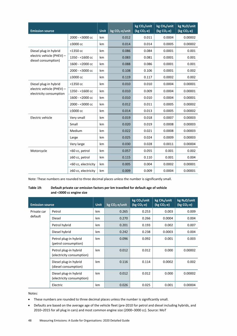
48 Measuring Emissions: A Guide for Organisations: 2020 Detailed Guide
Emission source Unit kg CO2-e/unit
kg CO2/unit
(kg CO2-e)
kg CH4/unit
(kg CO2-e)
kg N2O/unit
(kg CO2-e)
2000 - <3000 cc km 0.012 0.011 0.0004 0.00002
≥3000 cc km 0.014 0.014 0.0005 0.00002
Diesel plug-in hybrid
electric vehicle (PHEV) –
diesel consumption)
<1350 cc km 0.086 0.084 0.0001 0.001
1350 - <1600 cc km 0.083 0.081 0.0001 0.001
1600 - <2000 cc km 0.088 0.086 0.0001 0.001
2000 - <3000 cc km 0.108 0.106 0.0001 0.002
≥3000 cc km 0.119 0.117 0.0002 0.002
Diesel plug-in hybrid
electric vehicle (PHEV) –
electricity consumption
<1350 cc km 0.010 0.010 0.0004 0.00001
1350 - <1600 cc km 0.010 0.009 0.0004 0.00001
1600 - <2000 cc km 0.010 0.010 0.0004 0.00001
2000 - <3000 cc km 0.012 0.011 0.0005 0.00002
≥3000 cc km 0.014 0.013 0.0005 0.00002
Electric vehicle Very small km 0.019 0.018 0.0007 0.00003
Small km 0.020 0.019 0.0008 0.00003
Medium km 0.022 0.021 0.0008 0.00003
Large km 0.025 0.024 0.0009 0.00003
Very large km 0.030 0.028 0.0011 0.00004
Motorcycle <60 cc, petrol km 0.057 0.055 0.001 0.002
≥60 cc, petrol km 0.115 0.110 0.001 0.004
<60 cc, electricity km 0.005 0.004 0.0002 0.00001
≥60 cc, electricity km 0.009 0.009 0.0004 0.00001
Note: These numbers are rounded to three decimal places unless the number is significantly small.
Table 19: Default private car emission factors per km travelled for default age of vehicle
and <3000 cc engine size
Emission source Unit kg CO2-e/unit kg CO2/unit (kg CO2-e)
kg CH4/unit (kg CO2-e)
kg N2O/unit (kg CO2-e)
Private car
default
Petrol km 0.265 0.253 0.003 0.009
Diesel km 0.270 0.266 0.0004 0.004
Petrol hybrid km 0.201 0.193 0.002 0.007
Diesel hybrid km 0.242 0.238 0.0003 0.004
Petrol plug-in hybrid
(petrol consumption)
km 0.096 0.092 0.001 0.003
Petrol plug-in hybrid
(electricity consumption)
km 0.012 0.012 0.000 0.00002
Diesel plug-in hybrid
(diesel consumption)
km 0.116 0.114 0.0002 0.002
Diesel plug-in hybrid
(electricity consumption)
km 0.012 0.012 0.000 0.00002
Electric km 0.026 0.025 0.001 0.00004
Notes:
• These numbers are rounded to three decimal places unless the number is significantly small.
• Defaults are based on the average age of the vehicle fleet (pre-2010 for petrol and diesel including hybrids, and
2010–2015 for all plug in cars) and most common engine size (2000–3000 cc). Source: MoT
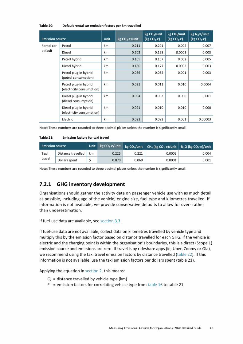
Measuring Emissions: A Guide for Organisations: 2020 Detailed Guide 49
Table 20: Default rental car emission factors per km travelled
Emission source Unit kg CO2-e/unit
kg CO2/unit
(kg CO2-e)
kg CH4/unit
(kg CO2-e)
kg N2O/unit
(kg CO2-e)
Rental car
default
Petrol km 0.211 0.201 0.002 0.007
Diesel km 0.202 0.198 0.0003 0.003
Petrol hybrid km 0.165 0.157 0.002 0.005
Diesel hybrid km 0.180 0.177 0.0002 0.003
Petrol plug-in hybrid
(petrol consumption)
km 0.086 0.082 0.001 0.003
Petrol plug-in hybrid
(electricity consumption)
km 0.021 0.011 0.010 0.0004
Diesel plug-in hybrid
(diesel consumption)
km 0.094 0.093 0.000 0.001
Diesel plug-in hybrid
(electricity consumption)
km 0.021 0.010 0.010 0.000
Electric km 0.023 0.022 0.001 0.00003
Note: These numbers are rounded to three decimal places unless the number is significantly small.
Table 21: Emission factors for taxi travel
Emission source Unit kg CO2-e/unit kg CO2/unit CH4 (kg CO2-e)/unit N2O (kg CO2-e)/unit
Taxi
travel
Distance travelled km 0.225 0.221 0.0003 0.004
Dollars spent $ 0.070 0.069 0.0001 0.001
Note: These numbers are rounded to three decimal places unless the number is significantly small.
7.2.1 GHG inventory development
Organisations should gather the activity data on passenger vehicle use with as much detail
as possible, including age of the vehicle, engine size, fuel type and kilometres travelled. If
information is not available, we provide conservative defaults to allow for over- rather
than underestimation.
If fuel-use data are available, see section 3.3.
If fuel-use data are not available, collect data on kilometres travelled by vehicle type and
multiply this by the emission factor based on distance travelled for each GHG. If the vehicle is
electric and the charging point is within the organisation’s boundaries, this is a direct (Scope 1)
emission source and emissions are zero. If travel is by rideshare apps (ie, Uber, Zoomy or Ola),
we recommend using the taxi travel emission factors by distance travelled (table 22). If this
information is not available, use the taxi emission factors per dollars spent (table 21).
Applying the equation in section 2, this means:
Q = distance travelled by vehicle type (km)
F = emission factors for correlating vehicle type from table 16 to table 21
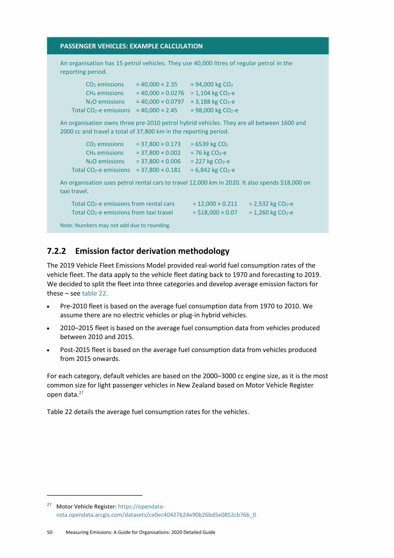
50 Measuring Emissions: A Guide for Organisations: 2020 Detailed Guide
PASSENGER VEHICLES: EXAMPLE CALCULATION
An organisation has 15 petrol vehicles. They use 40,000 litres of regular petrol in the
reporting period.
CO2 emissions = 40,000 × 2.35 = 94,000 kg CO2
CH4 emissions = 40,000 × 0.0276 = 1,104 kg CO2-e
N2O emissions = 40,000 × 0.0797 = 3,188 kg CO2-e
Total CO2-e emissions = 40,000 × 2.45 = 98,000 kg CO2-e
An organisation owns three pre-2010 petrol hybrid vehicles. They are all between 1600 and
2000 cc and travel a total of 37,800 km in the reporting period.
CO2 emissions = 37,800 × 0.173 = 6539 kg CO2
CH4 emissions = 37,800 × 0.002 = 76 kg CO2-e
N2O emissions = 37,800 × 0.006 = 227 kg CO2-e
Total CO2-e emissions = 37,800 × 0.181 = 6,842 kg CO2-e
An organisation uses petrol rental cars to travel 12,000 km in 2020. It also spends $18,000 on
taxi travel.
Total CO2-e emissions from rental cars = 12,000 × 0.211 = 2,532 kg CO2-e
Total CO2-e emissions from taxi travel = $18,000 × 0.07 = 1,260 kg CO2-e
Note: Numbers may not add due to rounding.
7.2.2 Emission factor derivation methodology
The 2019 Vehicle Fleet Emissions Model provided real-world fuel consumption rates of the
vehicle fleet. The data apply to the vehicle fleet dating back to 1970 and forecasting to 2019.
We decided to split the fleet into three categories and develop average emission factors for
these – see table 22.
• Pre-2010 fleet is based on the average fuel consumption data from 1970 to 2010. We assume there are no electric vehicles or plug-in hybrid vehicles.
• 2010–2015 fleet is based on the average fuel consumption data from vehicles produced between 2010 and 2015.
• Post-2015 fleet is based on the average fuel consumption data from vehicles produced from 2015 onwards.
For each category, default vehicles are based on the 2000–3000 cc engine size, as it is the most
common size for light passenger vehicles in New Zealand based on Motor Vehicle Register
open data.27
Table 22 details the average fuel consumption rates for the vehicles.
27 Motor Vehicle Register: https://opendata-
nzta.opendata.arcgis.com/datasets/ce0ec40427b24e90b26bd5e0852cb76b_0
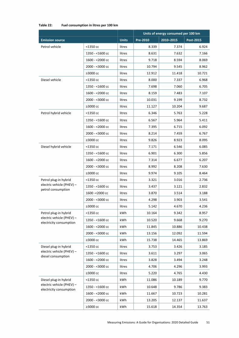
Measuring Emissions: A Guide for Organisations: 2020 Detailed Guide 51
Table 22: Fuel consumption in litres per 100 km
Units of energy consumed per 100 km
Emission source Units Pre-2010 2010–2015 Post-2015
Petrol vehicle <1350 cc litres 8.339 7.374 6.924
1350 - <1600 cc litres 8.631 7.632 7.166
1600 - <2000 cc litres 9.718 8.594 8.069
2000 - <3000 cc litres 10.794 9.545 8.962
≥3000 cc litres 12.912 11.418 10.721
Diesel vehicle <1350 cc litres 8.000 7.337 6.968
1350 - <1600 cc litres 7.698 7.060 6.705
1600 - <2000 cc litres 8.159 7.483 7.107
2000 - <3000 cc litres 10.031 9.199 8.732
≥3000 cc litres 11.127 10.204 9.687
Petrol hybrid vehicle <1350 cc litres 6.346 5.763 5.228
1350 - <1600 cc litres 6.567 5.964 5.411
1600 - <2000 cc litres 7.395 6.715 6.092
2000 - <3000 cc litres 8.214 7.459 6.767
≥3000 cc litres 9.826 8.923 8.095
Diesel hybrid vehicle <1350 cc litres 7.171 6.546 6.085
1350 - <1600 cc litres 6.901 6.300 5.856
1600 - <2000 cc litres 7.314 6.677 6.207
2000 - <3000 cc litres 8.992 8.208 7.630
≥3000 cc litres 9.974 9.105 8.464
Petrol plug-in hybrid
electric vehicle (PHEV) –
petrol consumption
<1350 cc litres 3.321 3.016 2.736
1350 - <1600 cc litres 3.437 3.121 2.832
1600 -<2000 cc litres 3.870 3.514 3.188
2000 - <3000 cc litres 4.298 3.903 3.541
≥3000 cc litres 5.142 4.670 4.236
Petrol plug-in hybrid
electric vehicle (PHEV) –
electricity consumption
<1350 cc kWh 10.164 9.342 8.957
1350 - <1600 cc kWh 10.520 9.668 9.270
1600 - <2000 cc kWh 11.845 10.886 10.438
2000 - <3000 cc kWh 13.156 12.092 11.594
≥3000 cc kWh 15.738 14.465 13.869
Diesel plug-in hybrid
electric vehicle (PHEV) –
diesel consumption
<1350 cc litres 3.753 3.426 3.185
1350 - <1600 cc litres 3.611 3.297 3.065
1600 - <2000 cc litres 3.828 3.494 3.248
2000 - <3000 cc litres 4.706 4.296 3.993
≥3000 cc litres 5.220 4.765 4.430
Diesel plug-in hybrid
electric vehicle (PHEV) –
electricity consumption
<1350 cc kWh 11.086 10.189 9.770
1350 - <1600 cc kWh 10.648 9.786 9.383
1600 - <2000 cc kWh 11.667 10.723 10.281
2000 - <3000 cc kWh 13.205 12.137 11.637
≥3000 cc kWh 15.618 14.354 13.763
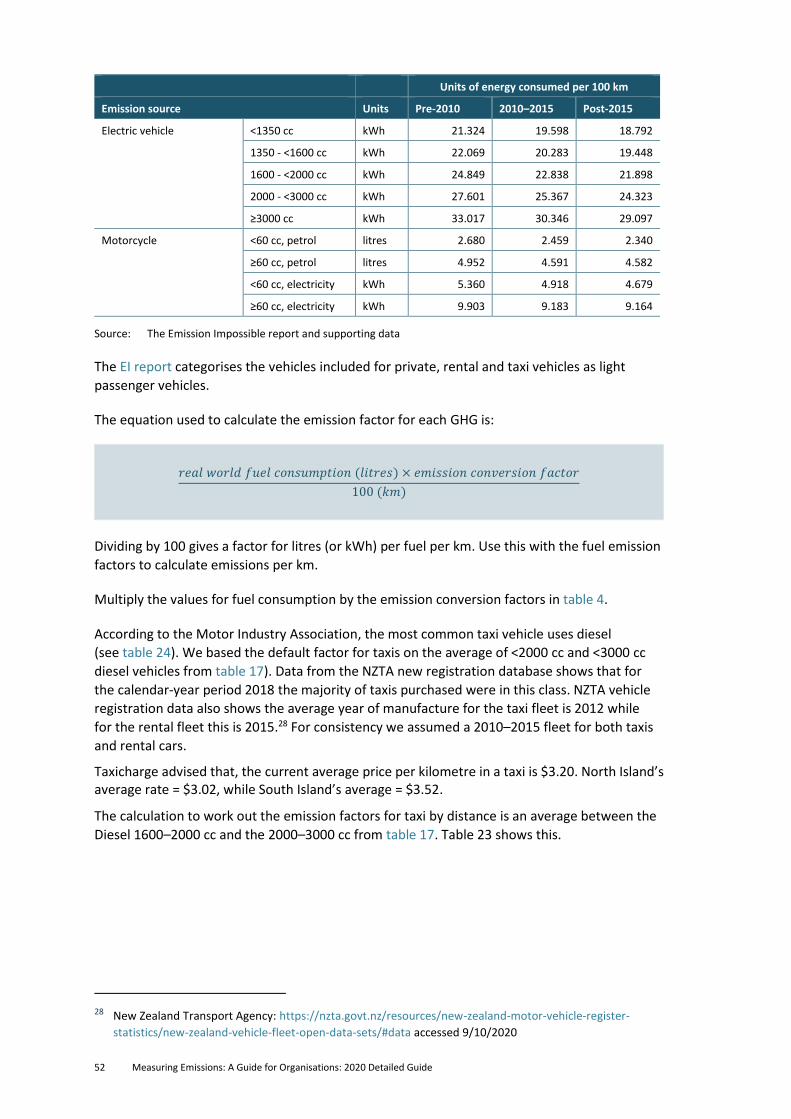
52 Measuring Emissions: A Guide for Organisations: 2020 Detailed Guide
Units of energy consumed per 100 km
Emission source Units Pre-2010 2010–2015 Post-2015
Electric vehicle <1350 cc kWh 21.324 19.598 18.792
1350 - <1600 cc kWh 22.069 20.283 19.448
1600 - <2000 cc kWh 24.849 22.838 21.898
2000 - <3000 cc kWh 27.601 25.367 24.323
≥3000 cc kWh 33.017 30.346 29.097
Motorcycle <60 cc, petrol litres 2.680 2.459 2.340
≥60 cc, petrol litres 4.952 4.591 4.582
<60 cc, electricity kWh 5.360 4.918 4.679
≥60 cc, electricity kWh 9.903 9.183 9.164
Source: The Emission Impossible report and supporting data
The EI report categorises the vehicles included for private, rental and taxi vehicles as light
passenger vehicles.
The equation used to calculate the emission factor for each GHG is:
𝑟𝑒𝑎𝑙 𝑤𝑜𝑟𝑙𝑑 𝑓𝑢𝑒𝑙 𝑐𝑜𝑛𝑠𝑢𝑚𝑝𝑡𝑖𝑜𝑛 (𝑙𝑖𝑡𝑟𝑒𝑠) × 𝑒𝑚𝑖𝑠𝑠𝑖𝑜𝑛 𝑐𝑜𝑛𝑣𝑒𝑟𝑠𝑖𝑜𝑛 𝑓𝑎𝑐𝑡𝑜𝑟
100 (𝑘𝑚)
Dividing by 100 gives a factor for litres (or kWh) per fuel per km. Use this with the fuel emission
factors to calculate emissions per km.
Multiply the values for fuel consumption by the emission conversion factors in table 4.
According to the Motor Industry Association, the most common taxi vehicle uses diesel
(see table 24). We based the default factor for taxis on the average of <2000 cc and <3000 cc
diesel vehicles from table 17). Data from the NZTA new registration database shows that for
the calendar-year period 2018 the majority of taxis purchased were in this class. NZTA vehicle
registration data also shows the average year of manufacture for the taxi fleet is 2012 while
for the rental fleet this is 2015.28 For consistency we assumed a 2010–2015 fleet for both taxis
and rental cars.
Taxicharge advised that, the current average price per kilometre in a taxi is $3.20. North Island’s average rate = $3.02, while South Island’s average = $3.52.
The calculation to work out the emission factors for taxi by distance is an average between the
Diesel 1600–2000 cc and the 2000–3000 cc from table 17. Table 23 shows this.
28 New Zealand Transport Agency: https://nzta.govt.nz/resources/new-zealand-motor-vehicle-register-
statistics/new-zealand-vehicle-fleet-open-data-sets/#data accessed 9/10/2020
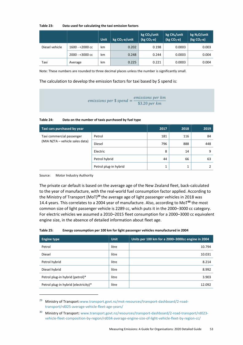
Measuring Emissions: A Guide for Organisations: 2020 Detailed Guide 53
Table 23: Data used for calculating the taxi emission factors
Unit kg CO2-e/unit
kg CO2/unit
(kg CO2-e)
kg CH4/unit
(kg CO2-e)
kg N2O/unit
(kg CO2-e)
Diesel vehicle 1600 - <2000 cc km 0.202 0.198 0.0003 0.003
2000 - <3000 cc km 0.248 0.244 0.0003 0.004
Taxi Average km 0.225 0.221 0.0003 0.004
Note: These numbers are rounded to three decimal places unless the number is significantly small.
The calculation to develop the emission factors for taxi based by $ spend is:
𝑒𝑚𝑖𝑠𝑠𝑖𝑜𝑛𝑠 𝑝𝑒𝑟 $ 𝑠𝑝𝑒𝑛𝑑 =𝑒𝑚𝑖𝑠𝑠𝑖𝑜𝑛𝑠 𝑝𝑒𝑟 𝑘𝑚
$3.20 𝑝𝑒𝑟 𝑘𝑚
Table 24: Data on the number of taxis purchased by fuel type
Taxi cars purchased by year 2017 2018 2019
Taxi commercial passenger
(MIA NZTA – vehicle sales data)
Petrol 181 116 84
Diesel 796 888 448
Electric 8 14 9
Petrol hybrid 44 66 63
Petrol plug-in hybrid 1 1 2
Source: Motor Industry Authority
The private car default is based on the average age of the New Zealand fleet, back-calculated
to the year of manufacture, with the real-world fuel consumption factor applied. According to
the Ministry of Transport (MoT)29 the average age of light passenger vehicles in 2018 was
14.4 years. This correlates to a 2004 year of manufacture. Also, according to MoT30 the most
common size of light passenger vehicle is 2289 cc, which puts it in the 2000–3000 cc category.
For electric vehicles we assumed a 2010–2015 fleet consumption for a 2000–3000 cc equivalent
engine size, in the absence of detailed information about fleet age.
Table 25: Energy consumption per 100 km for light passenger vehicles manufactured in 2004
Engine type Unit Units per 100 km for a 2000–3000cc engine in 2004
Petrol litre 10.794
Diesel litre 10.031
Petrol hybrid litre 8.214
Diesel hybrid litre 8.992
Petrol plug-in hybrid (petrol)* litre 3.903
Petrol plug-in hybrid (electricity)* litre 12.092
29 Ministry of Transport: www.transport.govt.nz/mot-resources/transport-dashboard/2-road-
transport/rd025-average-vehicle-fleet-age-years/
30 Ministry of Transport: www.transport.govt.nz/resources/transport-dashboard/2-road-transport/rd023-
vehicle-fleet-composition-by-region/rd034-average-engine-size-of-light-vehicle-fleet-by-region-cc/
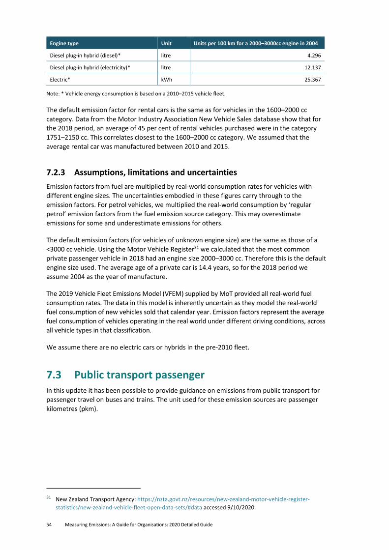
54 Measuring Emissions: A Guide for Organisations: 2020 Detailed Guide
Engine type Unit Units per 100 km for a 2000–3000cc engine in 2004
Diesel plug-in hybrid (diesel)* litre 4.296
Diesel plug-in hybrid (electricity)* litre 12.137
Electric* kWh 25.367
Note: * Vehicle energy consumption is based on a 2010–2015 vehicle fleet.
The default emission factor for rental cars is the same as for vehicles in the 1600–2000 cc
category. Data from the Motor Industry Association New Vehicle Sales database show that for
the 2018 period, an average of 45 per cent of rental vehicles purchased were in the category
1751–2150 cc. This correlates closest to the 1600–2000 cc category. We assumed that the
average rental car was manufactured between 2010 and 2015.
7.2.3 Assumptions, limitations and uncertainties
Emission factors from fuel are multiplied by real-world consumption rates for vehicles with
different engine sizes. The uncertainties embodied in these figures carry through to the
emission factors. For petrol vehicles, we multiplied the real-world consumption by ‘regular
petrol’ emission factors from the fuel emission source category. This may overestimate
emissions for some and underestimate emissions for others.
The default emission factors (for vehicles of unknown engine size) are the same as those of a
<3000 cc vehicle. Using the Motor Vehicle Register31 we calculated that the most common
private passenger vehicle in 2018 had an engine size 2000–3000 cc. Therefore this is the default
engine size used. The average age of a private car is 14.4 years, so for the 2018 period we
assume 2004 as the year of manufacture.
The 2019 Vehicle Fleet Emissions Model (VFEM) supplied by MoT provided all real-world fuel
consumption rates. The data in this model is inherently uncertain as they model the real-world
fuel consumption of new vehicles sold that calendar year. Emission factors represent the average
fuel consumption of vehicles operating in the real world under different driving conditions, across
all vehicle types in that classification.
We assume there are no electric cars or hybrids in the pre-2010 fleet.
7.3 Public transport passenger In this update it has been possible to provide guidance on emissions from public transport for
passenger travel on buses and trains. The unit used for these emission sources are passenger
kilometres (pkm).
31 New Zealand Transport Agency: https://nzta.govt.nz/resources/new-zealand-motor-vehicle-register-
statistics/new-zealand-vehicle-fleet-open-data-sets/#data accessed 9/10/2020
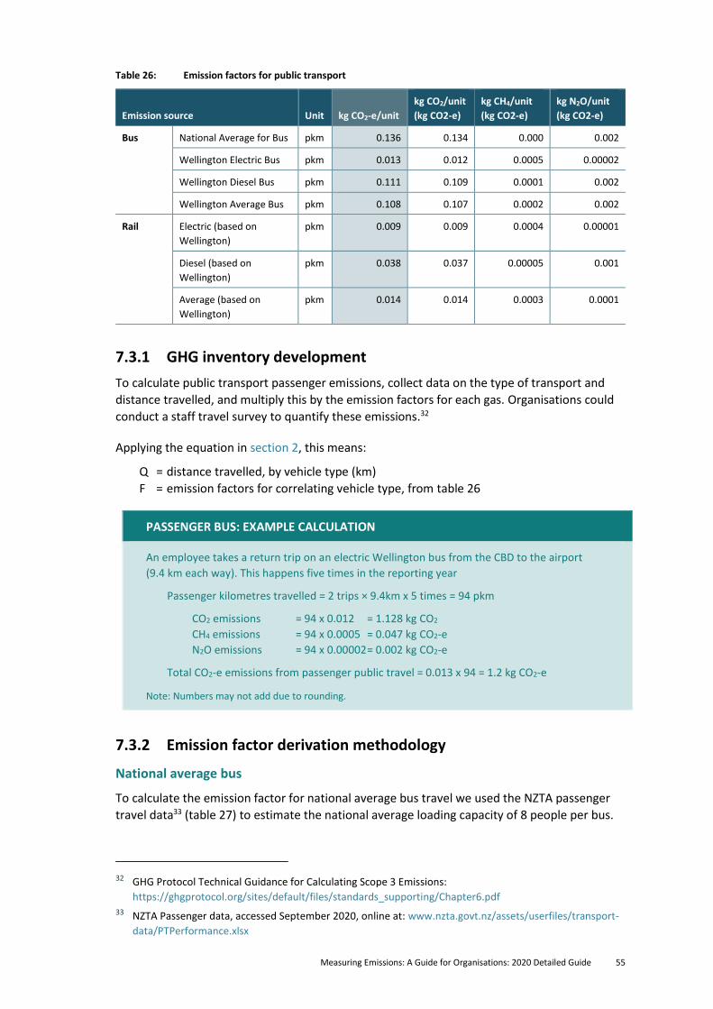
Measuring Emissions: A Guide for Organisations: 2020 Detailed Guide 55
Table 26: Emission factors for public transport
Emission source Unit kg CO2-e/unit
kg CO2/unit
(kg CO2-e)
kg CH4/unit
(kg CO2-e)
kg N2O/unit
(kg CO2-e)
Bus National Average for Bus pkm 0.136 0.134 0.000 0.002
Wellington Electric Bus pkm 0.013 0.012 0.0005 0.00002
Wellington Diesel Bus pkm 0.111 0.109 0.0001 0.002
Wellington Average Bus pkm 0.108 0.107 0.0002 0.002
Rail Electric (based on
Wellington)
pkm 0.009 0.009 0.0004 0.00001
Diesel (based on
Wellington)
pkm 0.038 0.037 0.00005 0.001
Average (based on
Wellington)
pkm 0.014 0.014 0.0003 0.0001
7.3.1 GHG inventory development
To calculate public transport passenger emissions, collect data on the type of transport and
distance travelled, and multiply this by the emission factors for each gas. Organisations could
conduct a staff travel survey to quantify these emissions.32
Applying the equation in section 2, this means:
Q = distance travelled, by vehicle type (km)
F = emission factors for correlating vehicle type, from table 26
PASSENGER BUS: EXAMPLE CALCULATION
An employee takes a return trip on an electric Wellington bus from the CBD to the airport
(9.4 km each way). This happens five times in the reporting year
Passenger kilometres travelled = 2 trips × 9.4km x 5 times = 94 pkm
CO2 emissions = 94 x 0.012 = 1.128 kg CO2
CH4 emissions = 94 x 0.0005 = 0.047 kg CO2-e
N2O emissions = 94 x 0.00002 = 0.002 kg CO2-e
Total CO2-e emissions from passenger public travel = 0.013 x 94 = 1.2 kg CO2-e
Note: Numbers may not add due to rounding.
7.3.2 Emission factor derivation methodology
National average bus
To calculate the emission factor for national average bus travel we used the NZTA passenger
travel data33 (table 27) to estimate the national average loading capacity of 8 people per bus.
32 GHG Protocol Technical Guidance for Calculating Scope 3 Emissions:
https://ghgprotocol.org/sites/default/files/standards_supporting/Chapter6.pdf
33 NZTA Passenger data, accessed September 2020, online at: www.nzta.govt.nz/assets/userfiles/transport-
data/PTPerformance.xlsx
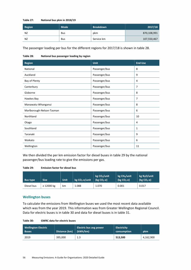
56 Measuring Emissions: A Guide for Organisations: 2020 Detailed Guide
Table 27: National bus pkm in 2018/19
Region Mode Breakdown 2017/18
NZ Bus pkm 870,108,991
NZ Bus Service km 107,550,467
The passenger loading per bus for the different regions for 2017/18 is shown in table 28.
Table 28: National bus passenger loading by region
Region Unit End Use
National Passenger/bus 8
Auckland Passenger/bus 9
Bay of Plenty Passenger/bus 4
Canterbury Passenger/bus 7
Gisborne Passenger/bus 8
Hawkes Bay Passenger/bus 7
Manawatu-Whanganui Passenger/bus 8
Marlborough-Nelson-Tasman Passenger/bus 6
Northland Passenger/bus 10
Otago Passenger/bus 4
Southland Passenger/bus 1
Taranaki Passenger/bus 9
Waikato Passenger/bus 6
Wellington Passenger/bus 11
We then divided the per km emission factor for diesel buses in table 29 by the national
passenger/bus loading rate to give the emissions per gas.
Table 29: Emission factor for diesel bus
Bus type Size Unit kg CO2-e/unit
kg CO2/unit
(kg CO2-e)
kg CH4/unit
(kg CO2-e)
kg N2O/unit
(kg CO2-e)
Diesel bus ≥ 12000 kg km 1.088 1.070 0.001 0.017
Wellington buses
To calculate the emissions from Wellington buses we used the most recent data available
which was from the year 2019. This information was from Greater Wellington Regional Council.
Data for electric buses is in table 30 and data for diesel buses is in table 31.
Table 30: GWRC data for electric buses
Wellington Electric
Buses Distance (km)
Electric bus avg power
(kWh/km)
Electricity
consumption pkm
2019 395,000 1.3 513,500 4,162,900
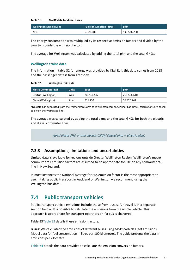
Measuring Emissions: A Guide for Organisations: 2020 Detailed Guide 57
Table 31: GWRC data for diesel buses
Wellington Diesel Buses Fuel consumption (litres) pkm
2019 5,923,000 143,526,200
The energy consumption was multiplied by its respective emission factors and divided by the
pkm to provide the emission factor.
The average for Wellington was calculated by adding the total pkm and the total GHGs.
Wellington trains data
The information in table 32 for energy was provided by Kiwi Rail, this data comes from 2018
and the passenger data is from Transdev.
Table 32: Wellington train data
Metro Commuter Rail Units 2018 pkm
Electric (Wellington) kWh 24,783,206 269,506,640
Diesel (Wellington) litres 811,253 57,925,242
*No data has been used from the Palmerston North to Wellington commuter line. For diesel, calculations are based
solely on the Wairarapa line.
The average was calculated by adding the total pkms and the total GHGs for both the electric
and diesel commuter lines.
(total diesel GHG + total electric GHG)/ (diesel pkm + electric pkm)
7.3.3 Assumptions, limitations and uncertainties
Limited data is available for regions outside Greater Wellington Region. Wellington’s metro
commuter rail emission factors are assumed to be appropriate for use on any commuter rail
line in New Zealand.
In most instances the National Average for Bus emission factor is the most appropriate to
use. If taking public transport in Auckland or Wellington we recommend using the
Wellington bus data.
7.4 Public transport vehicles Public transport vehicle emissions include those from buses. Air travel is in a separate
section below. It is possible to calculate the emissions from the whole vehicle. This
approach is appropriate for transport operators or if a bus is chartered.
Table 33Table 33 details these emission factors.
Buses: We calculated the emissions of different buses using MoT’s Vehicle Fleet Emissions
Model data for fuel consumption in litres per 100 kilometres. The guide presents the data in
emissions per kilometre.
Table 34 details the data provided to calculate the emission conversion factors.
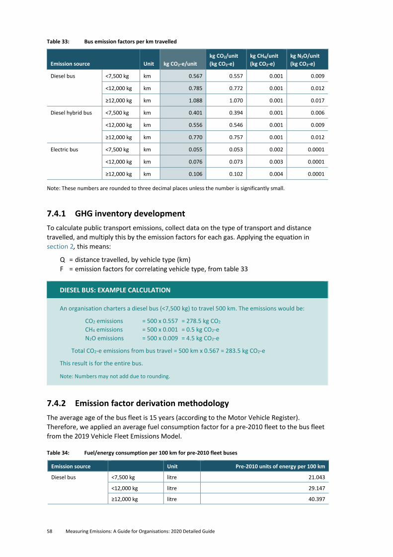
58 Measuring Emissions: A Guide for Organisations: 2020 Detailed Guide
Table 33: Bus emission factors per km travelled
Emission source Unit kg CO2-e/unit
kg CO2/unit
(kg CO2-e)
kg CH4/unit
(kg CO2-e)
kg N2O/unit
(kg CO2-e)
Diesel bus <7,500 kg km 0.567 0.557 0.001 0.009
<12,000 kg km 0.785 0.772 0.001 0.012
≥12,000 kg km 1.088 1.070 0.001 0.017
Diesel hybrid bus <7,500 kg km 0.401 0.394 0.001 0.006
<12,000 kg km 0.556 0.546 0.001 0.009
≥12,000 kg km 0.770 0.757 0.001 0.012
Electric bus <7,500 kg km 0.055 0.053 0.002 0.0001
<12,000 kg km 0.076 0.073 0.003 0.0001
≥12,000 kg km 0.106 0.102 0.004 0.0001
Note: These numbers are rounded to three decimal places unless the number is significantly small.
7.4.1 GHG inventory development
To calculate public transport emissions, collect data on the type of transport and distance
travelled, and multiply this by the emission factors for each gas. Applying the equation in
section 2, this means:
Q = distance travelled, by vehicle type (km)
F = emission factors for correlating vehicle type, from table 33
DIESEL BUS: EXAMPLE CALCULATION
An organisation charters a diesel bus (<7,500 kg) to travel 500 km. The emissions would be:
CO2 emissions = 500 x 0.557 = 278.5 kg CO2
CH4 emissions = 500 x 0.001 = 0.5 kg CO2-e
N2O emissions = 500 x 0.009 = 4.5 kg CO2-e
Total CO2-e emissions from bus travel = 500 km x 0.567 = 283.5 kg CO2-e
This result is for the entire bus.
Note: Numbers may not add due to rounding.
7.4.2 Emission factor derivation methodology
The average age of the bus fleet is 15 years (according to the Motor Vehicle Register).
Therefore, we applied an average fuel consumption factor for a pre-2010 fleet to the bus fleet
from the 2019 Vehicle Fleet Emissions Model.
Table 34: Fuel/energy consumption per 100 km for pre-2010 fleet buses
Emission source Unit Pre-2010 units of energy per 100 km
Diesel bus <7,500 kg litre 21.043
<12,000 kg litre 29.147
≥12,000 kg litre 40.397
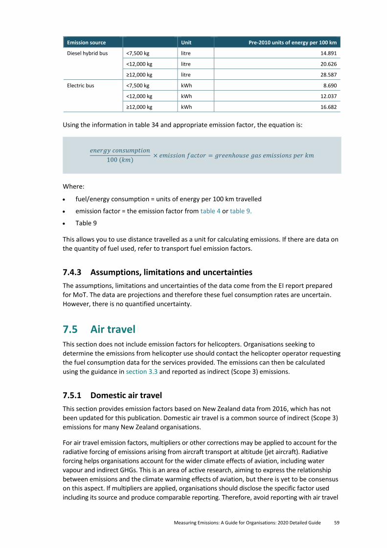
Measuring Emissions: A Guide for Organisations: 2020 Detailed Guide 59
Emission source Unit Pre-2010 units of energy per 100 km
Diesel hybrid bus <7,500 kg litre 14.891
<12,000 kg litre 20.626
≥12,000 kg litre 28.587
Electric bus <7,500 kg kWh 8.690
<12,000 kg kWh 12.037
≥12,000 kg kWh 16.682
Using the information in table 34 and appropriate emission factor, the equation is:
𝑒𝑛𝑒𝑟𝑔𝑦 𝑐𝑜𝑛𝑠𝑢𝑚𝑝𝑡𝑖𝑜𝑛
100 (𝑘𝑚) × 𝑒𝑚𝑖𝑠𝑠𝑖𝑜𝑛 𝑓𝑎𝑐𝑡𝑜𝑟 = 𝑔𝑟𝑒𝑒𝑛ℎ𝑜𝑢𝑠𝑒 𝑔𝑎𝑠 𝑒𝑚𝑖𝑠𝑠𝑖𝑜𝑛𝑠 𝑝𝑒𝑟 𝑘𝑚
Where:
• fuel/energy consumption = units of energy per 100 km travelled
• emission factor = the emission factor from table 4 or table 9.
• Table 9
This allows you to use distance travelled as a unit for calculating emissions. If there are data on
the quantity of fuel used, refer to transport fuel emission factors.
7.4.3 Assumptions, limitations and uncertainties
The assumptions, limitations and uncertainties of the data come from the EI report prepared
for MoT. The data are projections and therefore these fuel consumption rates are uncertain.
However, there is no quantified uncertainty.
7.5 Air travel This section does not include emission factors for helicopters. Organisations seeking to
determine the emissions from helicopter use should contact the helicopter operator requesting
the fuel consumption data for the services provided. The emissions can then be calculated
using the guidance in section 3.3 and reported as indirect (Scope 3) emissions.
7.5.1 Domestic air travel
This section provides emission factors based on New Zealand data from 2016, which has not
been updated for this publication. Domestic air travel is a common source of indirect (Scope 3)
emissions for many New Zealand organisations.
For air travel emission factors, multipliers or other corrections may be applied to account for the
radiative forcing of emissions arising from aircraft transport at altitude (jet aircraft). Radiative
forcing helps organisations account for the wider climate effects of aviation, including water
vapour and indirect GHGs. This is an area of active research, aiming to express the relationship
between emissions and the climate warming effects of aviation, but there is yet to be consensus
on this aspect. If multipliers are applied, organisations should disclose the specific factor used
including its source and produce comparable reporting. Therefore, avoid reporting with air travel
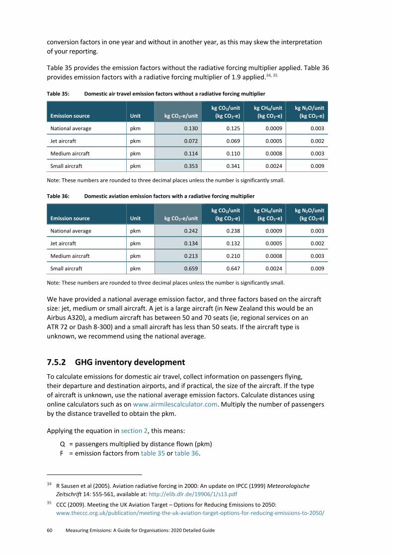
60 Measuring Emissions: A Guide for Organisations: 2020 Detailed Guide
conversion factors in one year and without in another year, as this may skew the interpretation
of your reporting.
Table 35 provides the emission factors without the radiative forcing multiplier applied. Table 36
provides emission factors with a radiative forcing multiplier of 1.9 applied.34, 35
Table 35: Domestic air travel emission factors without a radiative forcing multiplier
Emission source Unit kg CO2-e/unit
kg CO2/unit
(kg CO2-e)
kg CH4/unit
(kg CO2-e)
kg N2O/unit
(kg CO2-e)
National average pkm 0.130 0.125 0.0009 0.003
Jet aircraft pkm 0.072 0.069 0.0005 0.002
Medium aircraft pkm 0.114 0.110 0.0008 0.003
Small aircraft pkm 0.353 0.341 0.0024 0.009
Note: These numbers are rounded to three decimal places unless the number is significantly small.
Table 36: Domestic aviation emission factors with a radiative forcing multiplier
Emission source Unit kg CO2-e/unit
kg CO2/unit
(kg CO2-e)
kg CH4/unit
(kg CO2-e)
kg N2O/unit
(kg CO2-e)
National average pkm 0.242 0.238 0.0009 0.003
Jet aircraft pkm 0.134 0.132 0.0005 0.002
Medium aircraft pkm 0.213 0.210 0.0008 0.003
Small aircraft pkm 0.659 0.647 0.0024 0.009
Note: These numbers are rounded to three decimal places unless the number is significantly small.
We have provided a national average emission factor, and three factors based on the aircraft
size: jet, medium or small aircraft. A jet is a large aircraft (in New Zealand this would be an
Airbus A320), a medium aircraft has between 50 and 70 seats (ie, regional services on an
ATR 72 or Dash 8-300) and a small aircraft has less than 50 seats. If the aircraft type is
unknown, we recommend using the national average.
7.5.2 GHG inventory development
To calculate emissions for domestic air travel, collect information on passengers flying,
their departure and destination airports, and if practical, the size of the aircraft. If the type
of aircraft is unknown, use the national average emission factors. Calculate distances using
online calculators such as on www.airmilescalculator.com. Multiply the number of passengers
by the distance travelled to obtain the pkm.
Applying the equation in section 2, this means:
Q = passengers multiplied by distance flown (pkm)
F = emission factors from table 35 or table 36.
34 R Sausen et al (2005). Aviation radiative forcing in 2000: An update on IPCC (1999) Meteorologische
Zeitschrift 14: 555-561, available at: http://elib.dlr.de/19906/1/s13.pdf
35 CCC (2009). Meeting the UK Aviation Target – Options for Reducing Emissions to 2050:
www.theccc.org.uk/publication/meeting-the-uk-aviation-target-options-for-reducing-emissions-to-2050/
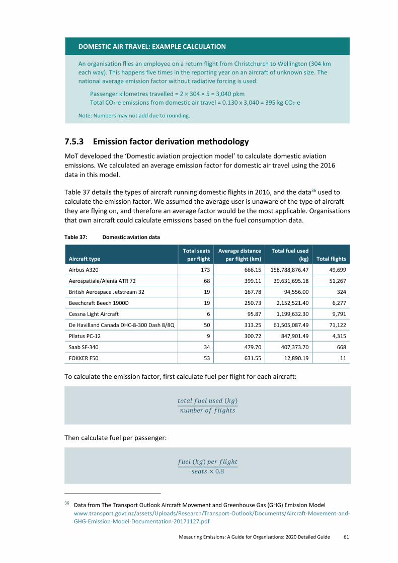
Measuring Emissions: A Guide for Organisations: 2020 Detailed Guide 61
DOMESTIC AIR TRAVEL: EXAMPLE CALCULATION
An organisation flies an employee on a return flight from Christchurch to Wellington (304 km
each way). This happens five times in the reporting year on an aircraft of unknown size. The
national average emission factor without radiative forcing is used.
Passenger kilometres travelled = 2 × 304 × 5 = 3,040 pkm
Total CO2-e emissions from domestic air travel = 0.130 x 3,040 = 395 kg CO2-e
Note: Numbers may not add due to rounding.
7.5.3 Emission factor derivation methodology
MoT developed the ‘Domestic aviation projection model’ to calculate domestic aviation
emissions. We calculated an average emission factor for domestic air travel using the 2016
data in this model.
Table 37 details the types of aircraft running domestic flights in 2016, and the data36 used to
calculate the emission factor. We assumed the average user is unaware of the type of aircraft
they are flying on, and therefore an average factor would be the most applicable. Organisations
that own aircraft could calculate emissions based on the fuel consumption data.
Table 37: Domestic aviation data
Aircraft type
Total seats
per flight
Average distance
per flight (km)
Total fuel used
(kg) Total flights
Airbus A320 173 666.15 158,788,876.47 49,699
Aerospatiale/Alenia ATR 72 68 399.11 39,631,695.18 51,267
British Aerospace Jetstream 32 19 167.78 94,556.00 324
Beechcraft Beech 1900D 19 250.73 2,152,521.40 6,277
Cessna Light Aircraft 6 95.87 1,199,632.30 9,791
De Havilland Canada DHC-8-300 Dash 8/8Q 50 313.25 61,505,087.49 71,122
Pilatus PC-12 9 300.72 847,901.49 4,315
Saab SF-340 34 479.70 407,373.70 668
FOKKER F50 53 631.55 12,890.19 11
To calculate the emission factor, first calculate fuel per flight for each aircraft:
𝑡𝑜𝑡𝑎𝑙 𝑓𝑢𝑒𝑙 𝑢𝑠𝑒𝑑 (𝑘𝑔)
𝑛𝑢𝑚𝑏𝑒𝑟 𝑜𝑓 𝑓𝑙𝑖𝑔ℎ𝑡𝑠
Then calculate fuel per passenger:
𝑓𝑢𝑒𝑙 (𝑘𝑔) 𝑝𝑒𝑟 𝑓𝑙𝑖𝑔ℎ𝑡
𝑠𝑒𝑎𝑡𝑠 × 0.8
36 Data from The Transport Outlook Aircraft Movement and Greenhouse Gas (GHG) Emission Model
www.transport.govt.nz/assets/Uploads/Research/Transport-Outlook/Documents/Aircraft-Movement-and-
GHG-Emission-Model-Documentation-20171127.pdf
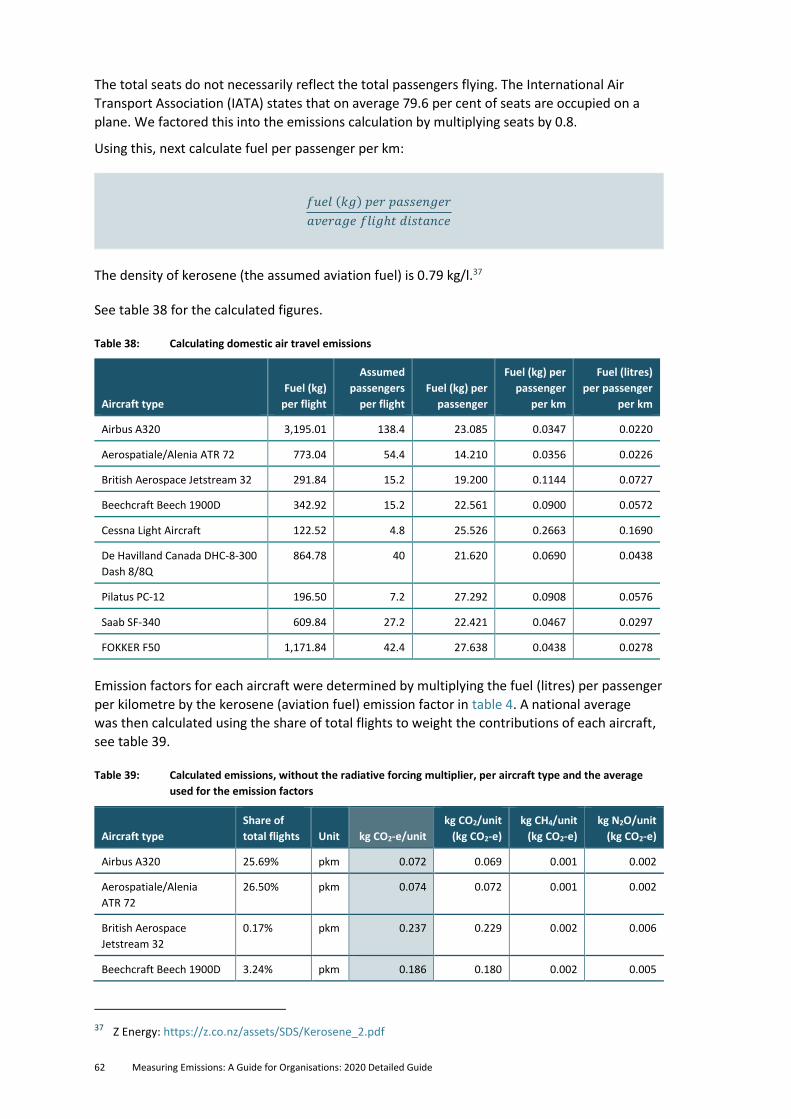
62 Measuring Emissions: A Guide for Organisations: 2020 Detailed Guide
The total seats do not necessarily reflect the total passengers flying. The International Air
Transport Association (IATA) states that on average 79.6 per cent of seats are occupied on a
plane. We factored this into the emissions calculation by multiplying seats by 0.8.
Using this, next calculate fuel per passenger per km:
𝑓𝑢𝑒𝑙 (𝑘𝑔) 𝑝𝑒𝑟 𝑝𝑎𝑠𝑠𝑒𝑛𝑔𝑒𝑟
𝑎𝑣𝑒𝑟𝑎𝑔𝑒 𝑓𝑙𝑖𝑔ℎ𝑡 𝑑𝑖𝑠𝑡𝑎𝑛𝑐𝑒
The density of kerosene (the assumed aviation fuel) is 0.79 kg/l.37
See table 38 for the calculated figures.
Table 38: Calculating domestic air travel emissions
Aircraft type
Fuel (kg)
per flight
Assumed
passengers
per flight
Fuel (kg) per
passenger
Fuel (kg) per
passenger
per km
Fuel (litres)
per passenger
per km
Airbus A320 3,195.01 138.4 23.085 0.0347 0.0220
Aerospatiale/Alenia ATR 72 773.04 54.4 14.210 0.0356 0.0226
British Aerospace Jetstream 32 291.84 15.2 19.200 0.1144 0.0727
Beechcraft Beech 1900D 342.92 15.2 22.561 0.0900 0.0572
Cessna Light Aircraft 122.52 4.8 25.526 0.2663 0.1690
De Havilland Canada DHC-8-300
Dash 8/8Q
864.78 40 21.620 0.0690 0.0438
Pilatus PC-12 196.50 7.2 27.292 0.0908 0.0576
Saab SF-340 609.84 27.2 22.421 0.0467 0.0297
FOKKER F50 1,171.84 42.4 27.638 0.0438 0.0278
Emission factors for each aircraft were determined by multiplying the fuel (litres) per passenger
per kilometre by the kerosene (aviation fuel) emission factor in table 4. A national average
was then calculated using the share of total flights to weight the contributions of each aircraft,
see table 39.
Table 39: Calculated emissions, without the radiative forcing multiplier, per aircraft type and the average
used for the emission factors
Aircraft type
Share of
total flights Unit kg CO2-e/unit
kg CO2/unit
(kg CO2-e)
kg CH4/unit
(kg CO2-e)
kg N2O/unit
(kg CO2-e)
Airbus A320 25.69% pkm 0.072 0.069 0.001 0.002
Aerospatiale/Alenia
ATR 72
26.50% pkm 0.074 0.072 0.001 0.002
British Aerospace
Jetstream 32
0.17% pkm 0.237 0.229 0.002 0.006
Beechcraft Beech 1900D 3.24% pkm 0.186 0.180 0.002 0.005
37 Z Energy: https://z.co.nz/assets/SDS/Kerosene_2.pdf
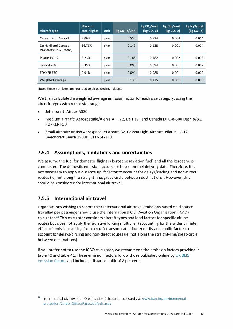
Measuring Emissions: A Guide for Organisations: 2020 Detailed Guide 63
Aircraft type
Share of
total flights Unit kg CO2-e/unit
kg CO2/unit
(kg CO2-e)
kg CH4/unit
(kg CO2-e)
kg N2O/unit
(kg CO2-e)
Cessna Light Aircraft 5.06% pkm 0.552 0.534 0.004 0.014
De Havilland Canada
DHC-8-300 Dash 8/8Q
36.76% pkm 0.143 0.138 0.001 0.004
Pilatus PC-12 2.23% pkm 0.188 0.182 0.002 0.005
Saab SF-340 0.35% pkm 0.097 0.094 0.001 0.002
FOKKER F50 0.01% pkm 0.091 0.088 0.001 0.002
Weighted average pkm 0.130 0.125 0.001 0.003
Note: These numbers are rounded to three decimal places.
We then calculated a weighted average emission factor for each size category, using the
aircraft types within that size range:
• Jet aircraft: Airbus A320
• Medium aircraft: Aerospatiale/Alenia ATR 72, De Havilland Canada DHC-8-300 Dash 8/8Q, FOKKER F50
• Small aircraft: British Aerospace Jetstream 32, Cessna Light Aircraft, Pilatus PC-12, Beechcraft Beech 1900D, Saab SF-340.
7.5.4 Assumptions, limitations and uncertainties
We assume the fuel for domestic flights is kerosene (aviation fuel) and all the kerosene is
combusted. The domestic emission factors are based on fuel delivery data. Therefore, it is
not necessary to apply a distance uplift factor to account for delays/circling and non-direct
routes (ie, not along the straight-line/great-circle between destinations). However, this
should be considered for international air travel.
7.5.5 International air travel
Organisations wishing to report their international air travel emissions based on distance
travelled per passenger should use the International Civil Aviation Organisation (ICAO)
calculator.38 This calculator considers aircraft types and load factors for specific airline
routes but does not apply the radiative forcing multiplier (accounting for the wider climate
effect of emissions arising from aircraft transport at altitude) or distance uplift factor to
account for delays/circling and non-direct routes (ie, not along the straight-line/great-circle
between destinations).
If you prefer not to use the ICAO calculator, we recommend the emission factors provided in
table 40 and table 41. These emission factors follow those published online by UK BEIS
emission factors and include a distance uplift of 8 per cent.
38 International Civil Aviation Organisation Calculator, accessed via: www.icao.int/environmental-
protection/CarbonOffset/Pages/default.aspx
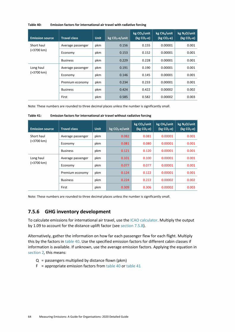
64 Measuring Emissions: A Guide for Organisations: 2020 Detailed Guide
Table 40: Emission factors for international air travel with radiative forcing
Emission source Travel class Unit kg CO2-e/unit
kg CO2/unit
(kg CO2-e)
kg CH4/unit
(kg CO2-e)
kg N2O/unit
(kg CO2-e)
Short haul
(<3700 km)
Average passenger pkm 0.156 0.155 0.00001 0.001
Economy pkm 0.153 0.152 0.00001 0.001
Business pkm 0.229 0.228 0.00001 0.001
Long haul
(>3700 km)
Average passenger pkm 0.191 0.190 0.00001 0.001
Economy pkm 0.146 0.145 0.00001 0.001
Premium economy pkm 0.234 0.233 0.00001 0.001
Business pkm 0.424 0.422 0.00002 0.002
First pkm 0.585 0.582 0.00002 0.003
Note: These numbers are rounded to three decimal places unless the number is significantly small.
Table 41: Emission factors for international air travel without radiative forcing
Emission source Travel class Unit kg CO2-e/unit
kg CO2/unit
(kg CO2-e)
kg CH4/unit
(kg CO2-e)
kg N2O/unit
(kg CO2-e)
Short haul
(<3700 km)
Average passenger pkm 0.082 0.081 0.00001 0.001
Economy pkm 0.081 0.080 0.00001 0.001
Business pkm 0.121 0.120 0.00001 0.001
Long haul
(>3700 km)
Average passenger pkm 0.101 0.100 0.00001 0.001
Economy pkm 0.077 0.077 0.00001 0.001
Premium economy pkm 0.124 0.122 0.00001 0.001
Business pkm 0.224 0.222 0.00002 0.002
First pkm 0.309 0.306 0.00002 0.003
Note: These numbers are rounded to three decimal places unless the number is significantly small.
7.5.6 GHG inventory development
To calculate emissions for international air travel, use the ICAO calculator. Multiply the output
by 1.09 to account for the distance uplift factor (see section 7.5.8).
Alternatively, gather the information on how far each passenger flew for each flight. Multiply
this by the factors in table 40. Use the specified emission factors for different cabin classes if
information is available. If unknown, use the average emission factors. Applying the equation in
section 2, this means:
Q = passengers multiplied by distance flown (pkm)
F = appropriate emission factors from table 40 or table 41
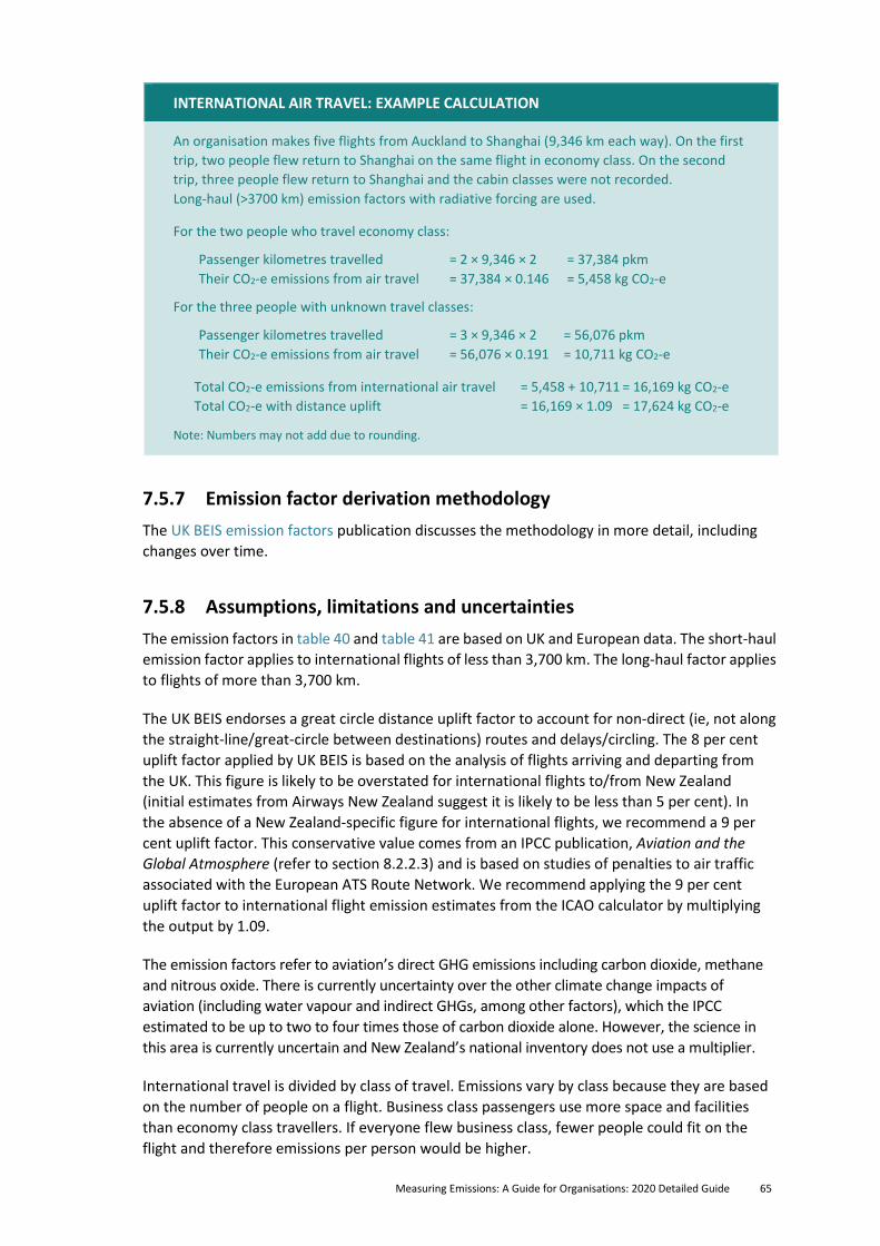
Measuring Emissions: A Guide for Organisations: 2020 Detailed Guide 65
INTERNATIONAL AIR TRAVEL: EXAMPLE CALCULATION
An organisation makes five flights from Auckland to Shanghai (9,346 km each way). On the first
trip, two people flew return to Shanghai on the same flight in economy class. On the second
trip, three people flew return to Shanghai and the cabin classes were not recorded.
Long-haul (>3700 km) emission factors with radiative forcing are used.
For the two people who travel economy class:
Passenger kilometres travelled = 2 × 9,346 × 2 = 37,384 pkm
Their CO2-e emissions from air travel = 37,384 × 0.146 = 5,458 kg CO2-e
For the three people with unknown travel classes:
Passenger kilometres travelled = 3 × 9,346 × 2 = 56,076 pkm
Their CO2-e emissions from air travel = 56,076 × 0.191 = 10,711 kg CO2-e
Total CO2-e emissions from international air travel = 5,458 + 10,711 = 16,169 kg CO2-e
Total CO2-e with distance uplift = 16,169 × 1.09 = 17,624 kg CO2-e
Note: Numbers may not add due to rounding.
7.5.7 Emission factor derivation methodology
The UK BEIS emission factors publication discusses the methodology in more detail, including
changes over time.
7.5.8 Assumptions, limitations and uncertainties
The emission factors in table 40 and table 41 are based on UK and European data. The short-haul
emission factor applies to international flights of less than 3,700 km. The long-haul factor applies
to flights of more than 3,700 km.
The UK BEIS endorses a great circle distance uplift factor to account for non-direct (ie, not along
the straight-line/great-circle between destinations) routes and delays/circling. The 8 per cent
uplift factor applied by UK BEIS is based on the analysis of flights arriving and departing from
the UK. This figure is likely to be overstated for international flights to/from New Zealand
(initial estimates from Airways New Zealand suggest it is likely to be less than 5 per cent). In
the absence of a New Zealand-specific figure for international flights, we recommend a 9 per
cent uplift factor. This conservative value comes from an IPCC publication, Aviation and the
Global Atmosphere (refer to section 8.2.2.3) and is based on studies of penalties to air traffic
associated with the European ATS Route Network. We recommend applying the 9 per cent
uplift factor to international flight emission estimates from the ICAO calculator by multiplying
the output by 1.09.
The emission factors refer to aviation’s direct GHG emissions including carbon dioxide, methane
and nitrous oxide. There is currently uncertainty over the other climate change impacts of
aviation (including water vapour and indirect GHGs, among other factors), which the IPCC
estimated to be up to two to four times those of carbon dioxide alone. However, the science in
this area is currently uncertain and New Zealand’s national inventory does not use a multiplier.
International travel is divided by class of travel. Emissions vary by class because they are based
on the number of people on a flight. Business class passengers use more space and facilities
than economy class travellers. If everyone flew business class, fewer people could fit on the
flight and therefore emissions per person would be higher.
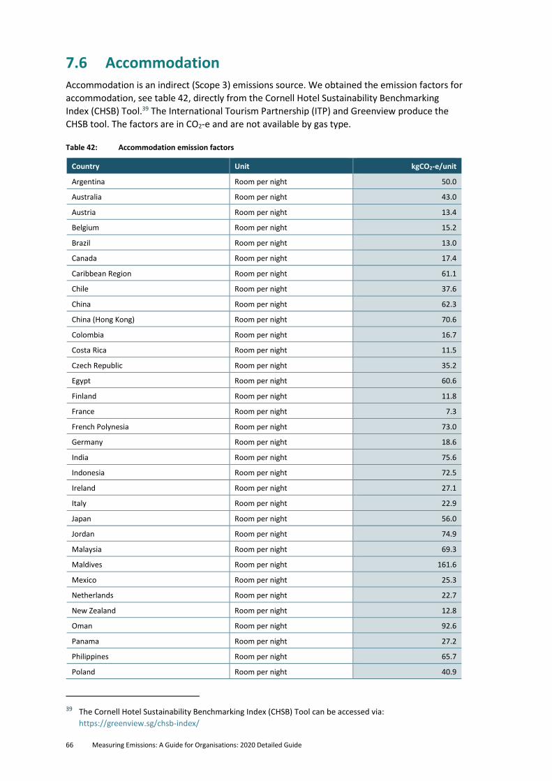
66 Measuring Emissions: A Guide for Organisations: 2020 Detailed Guide
7.6 Accommodation Accommodation is an indirect (Scope 3) emissions source. We obtained the emission factors for
accommodation, see table 42, directly from the Cornell Hotel Sustainability Benchmarking
Index (CHSB) Tool.39 The International Tourism Partnership (ITP) and Greenview produce the
CHSB tool. The factors are in CO2-e and are not available by gas type.
Table 42: Accommodation emission factors
Country Unit kgCO2-e/unit
Argentina Room per night 50.0
Australia Room per night 43.0
Austria Room per night 13.4
Belgium Room per night 15.2
Brazil Room per night 13.0
Canada Room per night 17.4
Caribbean Region Room per night 61.1
Chile Room per night 37.6
China Room per night 62.3
China (Hong Kong) Room per night 70.6
Colombia Room per night 16.7
Costa Rica Room per night 11.5
Czech Republic Room per night 35.2
Egypt Room per night 60.6
Finland Room per night 11.8
France Room per night 7.3
French Polynesia Room per night 73.0
Germany Room per night 18.6
India Room per night 75.6
Indonesia Room per night 72.5
Ireland Room per night 27.1
Italy Room per night 22.9
Japan Room per night 56.0
Jordan Room per night 74.9
Malaysia Room per night 69.3
Maldives Room per night 161.6
Mexico Room per night 25.3
Netherlands Room per night 22.7
New Zealand Room per night 12.8
Oman Room per night 92.6
Panama Room per night 27.2
Philippines Room per night 65.7
Poland Room per night 40.9
39 The Cornell Hotel Sustainability Benchmarking Index (CHSB) Tool can be accessed via:
https://greenview.sg/chsb-index/
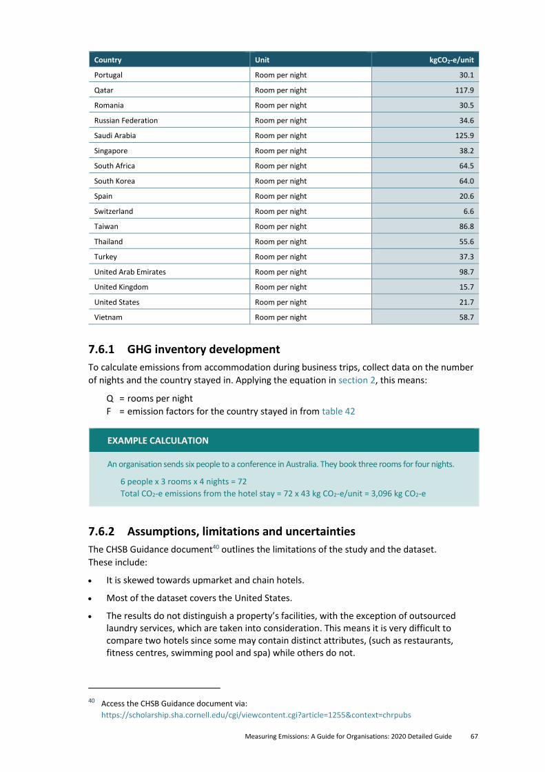
Measuring Emissions: A Guide for Organisations: 2020 Detailed Guide 67
Country Unit kgCO2-e/unit
Portugal Room per night 30.1
Qatar Room per night 117.9
Romania Room per night 30.5
Russian Federation Room per night 34.6
Saudi Arabia Room per night 125.9
Singapore Room per night 38.2
South Africa Room per night 64.5
South Korea Room per night 64.0
Spain Room per night 20.6
Switzerland Room per night 6.6
Taiwan Room per night 86.8
Thailand Room per night 55.6
Turkey Room per night 37.3
United Arab Emirates Room per night 98.7
United Kingdom Room per night 15.7
United States Room per night 21.7
Vietnam Room per night 58.7
7.6.1 GHG inventory development
To calculate emissions from accommodation during business trips, collect data on the number
of nights and the country stayed in. Applying the equation in section 2, this means:
Q = rooms per night
F = emission factors for the country stayed in from table 42
EXAMPLE CALCULATION
An organisation sends six people to a conference in Australia. They book three rooms for four nights.
6 people x 3 rooms x 4 nights = 72
Total CO2-e emissions from the hotel stay = 72 x 43 kg CO2-e/unit = 3,096 kg CO2-e
7.6.2 Assumptions, limitations and uncertainties
The CHSB Guidance document40 outlines the limitations of the study and the dataset.
These include:
• It is skewed towards upmarket and chain hotels.
• Most of the dataset covers the United States.
• The results do not distinguish a property’s facilities, with the exception of outsourced laundry services, which are taken into consideration. This means it is very difficult to compare two hotels since some may contain distinct attributes, (such as restaurants, fitness centres, swimming pool and spa) while others do not.
40 Access the CHSB Guidance document via:
https://scholarship.sha.cornell.edu/cgi/viewcontent.cgi?article=1255&context=chrpubs
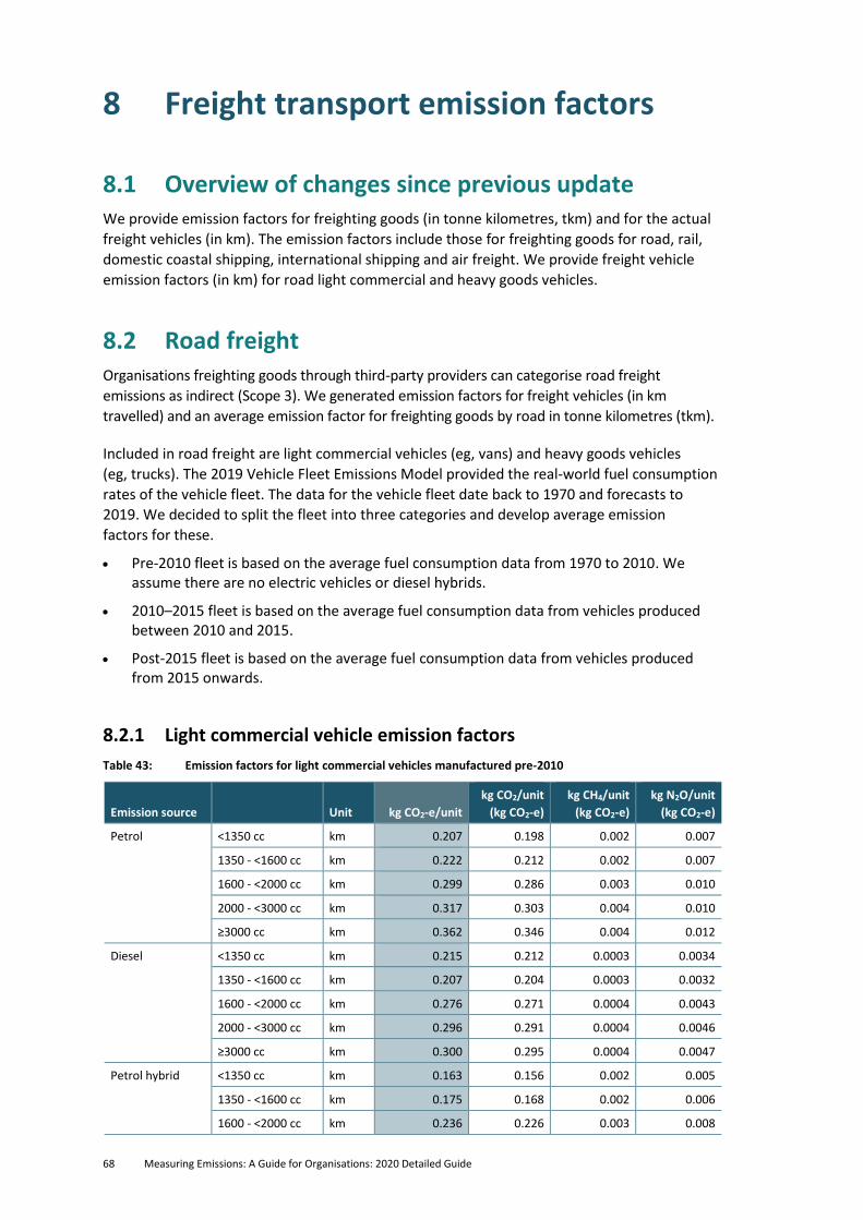
68 Measuring Emissions: A Guide for Organisations: 2020 Detailed Guide
8 Freight transport emission factors
8.1 Overview of changes since previous update We provide emission factors for freighting goods (in tonne kilometres, tkm) and for the actual
freight vehicles (in km). The emission factors include those for freighting goods for road, rail,
domestic coastal shipping, international shipping and air freight. We provide freight vehicle
emission factors (in km) for road light commercial and heavy goods vehicles.
8.2 Road freight Organisations freighting goods through third-party providers can categorise road freight
emissions as indirect (Scope 3). We generated emission factors for freight vehicles (in km
travelled) and an average emission factor for freighting goods by road in tonne kilometres (tkm).
Included in road freight are light commercial vehicles (eg, vans) and heavy goods vehicles
(eg, trucks). The 2019 Vehicle Fleet Emissions Model provided the real-world fuel consumption
rates of the vehicle fleet. The data for the vehicle fleet date back to 1970 and forecasts to
2019. We decided to split the fleet into three categories and develop average emission
factors for these.
• Pre-2010 fleet is based on the average fuel consumption data from 1970 to 2010. We assume there are no electric vehicles or diesel hybrids.
• 2010–2015 fleet is based on the average fuel consumption data from vehicles produced between 2010 and 2015.
• Post-2015 fleet is based on the average fuel consumption data from vehicles produced from 2015 onwards.
8.2.1 Light commercial vehicle emission factors
Table 43: Emission factors for light commercial vehicles manufactured pre-2010
Emission source Unit kg CO2-e/unit
kg CO2/unit
(kg CO2-e)
kg CH4/unit
(kg CO2-e)
kg N2O/unit
(kg CO2-e)
Petrol <1350 cc km 0.207 0.198 0.002 0.007
1350 - <1600 cc km 0.222 0.212 0.002 0.007
1600 - <2000 cc km 0.299 0.286 0.003 0.010
2000 - <3000 cc km 0.317 0.303 0.004 0.010
≥3000 cc km 0.362 0.346 0.004 0.012
Diesel <1350 cc km 0.215 0.212 0.0003 0.0034
1350 - <1600 cc km 0.207 0.204 0.0003 0.0032
1600 - <2000 cc km 0.276 0.271 0.0004 0.0043
2000 - <3000 cc km 0.296 0.291 0.0004 0.0046
≥3000 cc km 0.300 0.295 0.0004 0.0047
Petrol hybrid <1350 cc km 0.163 0.156 0.002 0.005
1350 - <1600 cc km 0.175 0.168 0.002 0.006
1600 - <2000 cc km 0.236 0.226 0.003 0.008
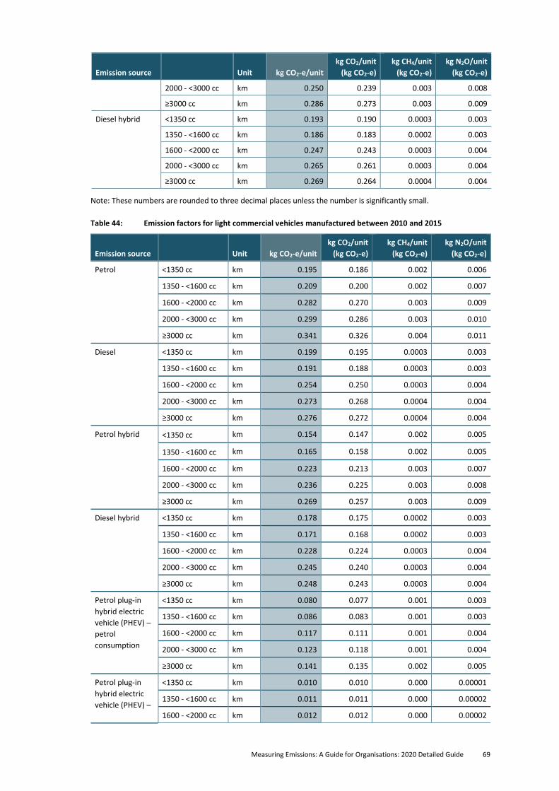
Measuring Emissions: A Guide for Organisations: 2020 Detailed Guide 69
Emission source Unit kg CO2-e/unit
kg CO2/unit
(kg CO2-e)
kg CH4/unit
(kg CO2-e)
kg N2O/unit
(kg CO2-e)
2000 - <3000 cc km 0.250 0.239 0.003 0.008
≥3000 cc km 0.286 0.273 0.003 0.009
Diesel hybrid <1350 cc km 0.193 0.190 0.0003 0.003
1350 - <1600 cc km 0.186 0.183 0.0002 0.003
1600 - <2000 cc km 0.247 0.243 0.0003 0.004
2000 - <3000 cc km 0.265 0.261 0.0003 0.004
≥3000 cc km 0.269 0.264 0.0004 0.004
Note: These numbers are rounded to three decimal places unless the number is significantly small.
Table 44: Emission factors for light commercial vehicles manufactured between 2010 and 2015
Emission source Unit kg CO2-e/unit
kg CO2/unit
(kg CO2-e)
kg CH4/unit
(kg CO2-e)
kg N2O/unit
(kg CO2-e)
Petrol <1350 cc km 0.195 0.186 0.002 0.006
1350 - <1600 cc km 0.209 0.200 0.002 0.007
1600 - <2000 cc km 0.282 0.270 0.003 0.009
2000 - <3000 cc km 0.299 0.286 0.003 0.010
≥3000 cc km 0.341 0.326 0.004 0.011
Diesel <1350 cc km 0.199 0.195 0.0003 0.003
1350 - <1600 cc km 0.191 0.188 0.0003 0.003
1600 - <2000 cc km 0.254 0.250 0.0003 0.004
2000 - <3000 cc km 0.273 0.268 0.0004 0.004
≥3000 cc km 0.276 0.272 0.0004 0.004
Petrol hybrid <1350 cc km 0.154 0.147 0.002 0.005
1350 - <1600 cc km 0.165 0.158 0.002 0.005
1600 - <2000 cc km 0.223 0.213 0.003 0.007
2000 - <3000 cc km 0.236 0.225 0.003 0.008
≥3000 cc km 0.269 0.257 0.003 0.009
Diesel hybrid <1350 cc km 0.178 0.175 0.0002 0.003
1350 - <1600 cc km 0.171 0.168 0.0002 0.003
1600 - <2000 cc km 0.228 0.224 0.0003 0.004
2000 - <3000 cc km 0.245 0.240 0.0003 0.004
≥3000 cc km 0.248 0.243 0.0003 0.004
Petrol plug-in
hybrid electric
vehicle (PHEV) –
petrol
consumption
<1350 cc km 0.080 0.077 0.001 0.003
1350 - <1600 cc km 0.086 0.083 0.001 0.003
1600 - <2000 cc km 0.117 0.111 0.001 0.004
2000 - <3000 cc km 0.123 0.118 0.001 0.004
≥3000 cc km 0.141 0.135 0.002 0.005
Petrol plug-in
hybrid electric
vehicle (PHEV) –
<1350 cc km 0.010 0.010 0.000 0.00001
1350 - <1600 cc km 0.011 0.011 0.000 0.00002
1600 - <2000 cc km 0.012 0.012 0.000 0.00002
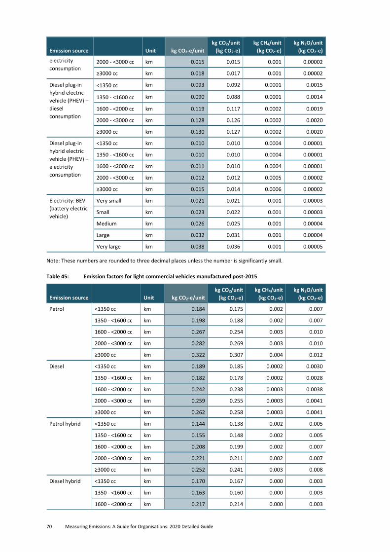
70 Measuring Emissions: A Guide for Organisations: 2020 Detailed Guide
Emission source Unit kg CO2-e/unit
kg CO2/unit
(kg CO2-e)
kg CH4/unit
(kg CO2-e)
kg N2O/unit
(kg CO2-e)
electricity
consumption 2000 - <3000 cc km 0.015 0.015 0.001 0.00002
≥3000 cc km 0.018 0.017 0.001 0.00002
Diesel plug-in
hybrid electric
vehicle (PHEV) –
diesel
consumption
<1350 cc km 0.093 0.092 0.0001 0.0015
1350 - <1600 cc km 0.090 0.088 0.0001 0.0014
1600 - <2000 cc km 0.119 0.117 0.0002 0.0019
2000 - <3000 cc km 0.128 0.126 0.0002 0.0020
≥3000 cc km 0.130 0.127 0.0002 0.0020
Diesel plug-in
hybrid electric
vehicle (PHEV) –
electricity
consumption
<1350 cc km 0.010 0.010 0.0004 0.00001
1350 - <1600 cc km 0.010 0.010 0.0004 0.00001
1600 - <2000 cc km 0.011 0.010 0.0004 0.00001
2000 - <3000 cc km 0.012 0.012 0.0005 0.00002
≥3000 cc km 0.015 0.014 0.0006 0.00002
Electricity: BEV
(battery electric
vehicle)
Very small km 0.021 0.021 0.001 0.00003
Small km 0.023 0.022 0.001 0.00003
Medium km 0.026 0.025 0.001 0.00004
Large km 0.032 0.031 0.001 0.00004
Very large km 0.038 0.036 0.001 0.00005
Note: These numbers are rounded to three decimal places unless the number is significantly small.
Table 45: Emission factors for light commercial vehicles manufactured post-2015
Emission source Unit kg CO2-e/unit
kg CO2/unit
(kg CO2-e)
kg CH4/unit
(kg CO2-e)
kg N2O/unit
(kg CO2-e)
Petrol <1350 cc km 0.184 0.175 0.002 0.007
1350 - <1600 cc km 0.198 0.188 0.002 0.007
1600 - <2000 cc km 0.267 0.254 0.003 0.010
2000 - <3000 cc km 0.282 0.269 0.003 0.010
≥3000 cc km 0.322 0.307 0.004 0.012
Diesel <1350 cc km 0.189 0.185 0.0002 0.0030
1350 - <1600 cc km 0.182 0.178 0.0002 0.0028
1600 - <2000 cc km 0.242 0.238 0.0003 0.0038
2000 - <3000 cc km 0.259 0.255 0.0003 0.0041
≥3000 cc km 0.262 0.258 0.0003 0.0041
Petrol hybrid <1350 cc km 0.144 0.138 0.002 0.005
1350 - <1600 cc km 0.155 0.148 0.002 0.005
1600 - <2000 cc km 0.208 0.199 0.002 0.007
2000 - <3000 cc km 0.221 0.211 0.002 0.007
≥3000 cc km 0.252 0.241 0.003 0.008
Diesel hybrid <1350 cc km 0.170 0.167 0.000 0.003
1350 - <1600 cc km 0.163 0.160 0.000 0.003
1600 - <2000 cc km 0.217 0.214 0.000 0.003
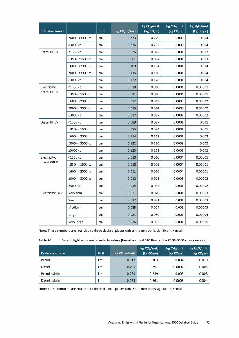
Measuring Emissions: A Guide for Organisations: 2020 Detailed Guide 71
Emission source Unit kg CO2-e/unit
kg CO2/unit
(kg CO2-e)
kg CH4/unit
(kg CO2-e)
kg N2O/unit
(kg CO2-e)
2000 - <3000 cc km 0.233 0.229 0.000 0.004
≥3000 cc km 0.236 0.232 0.000 0.004
Petrol PHEV <1350 cc km 0.075 0.072 0.001 0.002
1350 - <1600 cc km 0.081 0.077 0.001 0.003
1600 - <2000 cc km 0.109 0.104 0.001 0.004
2000 - <3000 cc km 0.115 0.110 0.001 0.004
≥3000 cc km 0.132 0.126 0.001 0.004
Electricity:
petrol PHEV
<1350 cc km 0.010 0.010 0.0004 0.00001
1350 - <1600 cc km 0.011 0.010 0.0004 0.00001
1600 - <2000 cc km 0.012 0.012 0.0005 0.00002
2000 - <3000 cc km 0.015 0.014 0.0006 0.00002
≥3000 cc km 0.017 0.017 0.0007 0.00002
Diesel PHEV <1350 cc km 0.089 0.087 0.0001 0.001
1350 - <1600 cc km 0.085 0.084 0.0001 0.001
1600 - <2000 cc km 0.114 0.112 0.0001 0.002
2000 - <3000 cc km 0.122 0.120 0.0002 0.002
≥3000 cc km 0.123 0.121 0.0002 0.002
Electricity:
diesel PHEV
<1350 cc km 0.010 0.010 0.0004 0.00001
1350 - <1600 cc km 0.010 0.009 0.0004 0.00001
1600 - <2000 cc km 0.011 0.010 0.0004 0.00001
2000 - <3000 cc km 0.012 0.011 0.0005 0.00002
≥3000 cc km 0.014 0.014 0.001 0.00002
Electricity: BEV Very small km 0.021 0.020 0.001 0.00003
Small km 0.022 0.021 0.001 0.00003
Medium km 0.025 0.024 0.001 0.00003
Large km 0.031 0.030 0.001 0.00004
Very large km 0.036 0.035 0.001 0.00005
Note: These numbers are rounded to three decimal places unless the number is significantly small.
Table 46: Default light commercial vehicle values (based on pre-2010 fleet and a 2000–3000 cc engine size)
Emission source Unit kg CO2-e/unit
kg CO2/unit
(kg CO2-e)
kg CH4/unit
(kg CO2-e)
kg N2O/unit
(kg CO2-e)
Petrol km 0.317 0.303 0.004 0.010
Diesel km 0.296 0.291 0.0004 0.005
Petrol hybrid km 0.250 0.239 0.003 0.008
Diesel hybrid km 0.265 0.261 0.0003 0.004
Note: These numbers are rounded to three decimal places unless the number is significantly small.
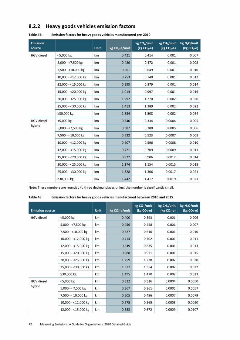
72 Measuring Emissions: A Guide for Organisations: 2020 Detailed Guide
8.2.2 Heavy goods vehicles emission factors
Table 47: Emission factors for heavy goods vehicles manufactured pre-2010
Emission
source Unit kg CO2-e/unit
kg CO2/unit
(kg CO2-e)
kg CH4/unit
(kg CO2-e)
kg N2O/unit
(kg CO2-e)
HGV diesel <5,000 kg km 0.421 0.414 0.001 0.007
5,000 - <7,500 kg km 0.480 0.472 0.001 0.008
7,500 - <10,000 kg km 0.661 0.649 0.001 0.010
10,000 - <12,000 kg km 0.753 0.740 0.001 0.012
12,000 - <15,000 kg km 0.895 0.879 0.001 0.014
15,000 - <20,000 kg km 1.014 0.997 0.001 0.016
20,000 - <25,000 kg km 1.292 1.270 0.002 0.020
25,000 - <30,000 kg km 1.413 1.389 0.002 0.022
≥30,000 kg km 1.534 1.508 0.002 0.024
HGV diesel
hybrid
<5,000 kg km 0.340 0.334 0.0004 0.005
5,000 - <7,500 kg km 0.387 0.380 0.0005 0.006
7,500 - <10,000 kg km 0.532 0.523 0.0007 0.008
10,000 - <12,000 kg km 0.607 0.596 0.0008 0.010
12,000 - <15,000 kg km 0.721 0.709 0.0009 0.011
15,000 - <20,000 kg km 0.922 0.906 0.0012 0.014
20,000 - <25,000 kg km 1.174 1.154 0.0015 0.018
25,000 - <30,000 kg km 1.328 1.306 0.0017 0.021
≥30,000 kg km 1.442 1.417 0.0019 0.023
Note: These numbers are rounded to three decimal places unless the number is significantly small.
Table 48: Emission factors for heavy goods vehicles manufactured between 2010 and 2015
Emission source Unit kg CO2-e/unit
kg CO2/unit
(kg CO2-e)
kg CH4/unit
(kg CO2-e)
kg N2O/unit
(kg CO2-e)
HGV diesel <5,000 kg km 0.400 0.393 0.001 0.006
5,000 - <7,500 kg km 0.456 0.448 0.001 0.007
7,500 - <10,000 kg km 0.627 0.616 0.001 0.010
10,000 - <12,000 kg km 0.714 0.702 0.001 0.011
12,000 - <15,000 kg km 0.849 0.835 0.001 0.013
15,000 - <20,000 kg km 0.988 0.971 0.001 0.015
20,000 - <25,000 kg km 1.259 1.238 0.002 0.020
25,000 - <30,000 kg km 1.377 1.354 0.002 0.022
≥30,000 kg km 1.495 1.470 0.002 0.023
HGV diesel
hybrid
<5,000 kg km 0.322 0.316 0.0004 0.0050
5,000 - <7,500 kg km 0.367 0.361 0.0005 0.0057
7,500 - <10,000 kg km 0.505 0.496 0.0007 0.0079
10,000 - <12,000 kg km 0.575 0.565 0.0008 0.0090
12,000 - <15,000 kg km 0.683 0.672 0.0009 0.0107
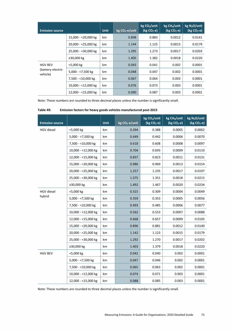
Measuring Emissions: A Guide for Organisations: 2020 Detailed Guide 73
Emission source Unit kg CO2-e/unit
kg CO2/unit
(kg CO2-e)
kg CH4/unit
(kg CO2-e)
kg N2O/unit
(kg CO2-e)
15,000 - <20,000 kg km 0.898 0.883 0.0012 0.0141
20,000 - <25,000 kg km 1.144 1.125 0.0015 0.0179
25,000 - <30,000 kg km 1.295 1.273 0.0017 0.0203
≥30,000 kg km 1.405 1.382 0.0018 0.0220
HGV BEV
(battery electric
vehicle)
<5,000 kg km 0.043 0.041 0.002 0.0001
5,000 - <7,500 kg km 0.048 0.047 0.002 0.0001
7,500 - <10,000 kg km 0.067 0.064 0.003 0.0001
10,000 - <12,000 kg km 0.076 0.073 0.003 0.0001
12,000 - <15,000 kg km 0.090 0.087 0.003 0.0001
Note: These numbers are rounded to three decimal places unless the number is significantly small.
Table 49: Emission factors for heavy goods vehicles manufactured post-2015
Emission source Unit kg CO2-e/unit
kg CO2/unit
(kg CO2-e)
kg CH4/unit
(kg CO2-e)
kg N2O/unit
(kg CO2-e)
HGV diesel <5,000 kg km 0.394 0.388 0.0005 0.0062
5,000 - <7,500 kg km 0.449 0.442 0.0006 0.0070
7,500 - <10,000 kg km 0.618 0.608 0.0008 0.0097
10,000 - <12,000 kg km 0.704 0.693 0.0009 0.0110
12,000 - <15,000 kg km 0.837 0.823 0.0011 0.0131
15,000 - <20,000 kg km 0.986 0.969 0.0013 0.0154
20,000 - <25,000 kg km 1.257 1.235 0.0017 0.0197
25,000 - <30,000 kg km 1.375 1.351 0.0018 0.0215
≥30,000 kg km 1.492 1.467 0.0020 0.0234
HGV diesel
hybrid
<5,000 kg km 0.315 0.309 0.0004 0.0049
5,000 - <7,500 kg km 0.359 0.353 0.0005 0.0056
7,500 - <10,000 kg km 0.493 0.485 0.0006 0.0077
10,000 - <12,000 kg km 0.562 0.553 0.0007 0.0088
12,000 - <15,000 kg km 0.668 0.657 0.0009 0.0105
15,000 - <20,000 kg km 0.896 0.881 0.0012 0.0140
20,000 - <25,000 kg km 1.142 1.123 0.0015 0.0179
25,000 - <30,000 kg km 1.292 1.270 0.0017 0.0202
≥30,000 kg km 1.403 1.379 0.0018 0.0220
HGV BEV <5,000 kg km 0.042 0.040 0.002 0.0001
5,000 - <7,500 kg km 0.047 0.046 0.002 0.0001
7,500 - <10,000 kg km 0.065 0.063 0.002 0.0001
10,000 - <12,000 kg km 0.074 0.071 0.003 0.0001
12,000 - <15,000 kg km 0.088 0.085 0.003 0.0001
Note: These numbers are rounded to three decimal places unless the number is significantly small.
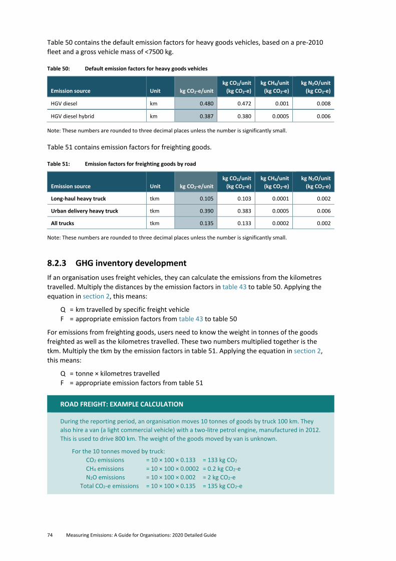
74 Measuring Emissions: A Guide for Organisations: 2020 Detailed Guide
Table 50 contains the default emission factors for heavy goods vehicles, based on a pre-2010
fleet and a gross vehicle mass of <7500 kg.
Table 50: Default emission factors for heavy goods vehicles
Emission source Unit kg CO2-e/unit
kg CO2/unit
(kg CO2-e)
kg CH4/unit
(kg CO2-e)
kg N2O/unit
(kg CO2-e)
HGV diesel km 0.480 0.472 0.001 0.008
HGV diesel hybrid km 0.387 0.380 0.0005 0.006
Note: These numbers are rounded to three decimal places unless the number is significantly small.
Table 51 contains emission factors for freighting goods.
Table 51: Emission factors for freighting goods by road
Emission source Unit kg CO2-e/unit
kg CO2/unit
(kg CO2-e)
kg CH4/unit
(kg CO2-e)
kg N2O/unit
(kg CO2-e)
Long-haul heavy truck tkm 0.105 0.103 0.0001 0.002
Urban delivery heavy truck tkm 0.390 0.383 0.0005 0.006
All trucks tkm 0.135 0.133 0.0002 0.002
Note: These numbers are rounded to three decimal places unless the number is significantly small.
8.2.3 GHG inventory development
If an organisation uses freight vehicles, they can calculate the emissions from the kilometres
travelled. Multiply the distances by the emission factors in table 43 to table 50. Applying the
equation in section 2, this means:
Q = km travelled by specific freight vehicle
F = appropriate emission factors from table 43 to table 50
For emissions from freighting goods, users need to know the weight in tonnes of the goods
freighted as well as the kilometres travelled. These two numbers multiplied together is the
tkm. Multiply the tkm by the emission factors in table 51. Applying the equation in section 2,
this means:
Q = tonne × kilometres travelled
F = appropriate emission factors from table 51
ROAD FREIGHT: EXAMPLE CALCULATION
During the reporting period, an organisation moves 10 tonnes of goods by truck 100 km. They
also hire a van (a light commercial vehicle) with a two-litre petrol engine, manufactured in 2012.
This is used to drive 800 km. The weight of the goods moved by van is unknown.
For the 10 tonnes moved by truck:
CO2 emissions = 10 × 100 × 0.133 = 133 kg CO2
CH4 emissions = 10 × 100 × 0.0002 = 0.2 kg CO2-e
N2O emissions = 10 × 100 × 0.002 = 2 kg CO2-e
Total CO2-e emissions = 10 × 100 × 0.135 = 135 kg CO2-e
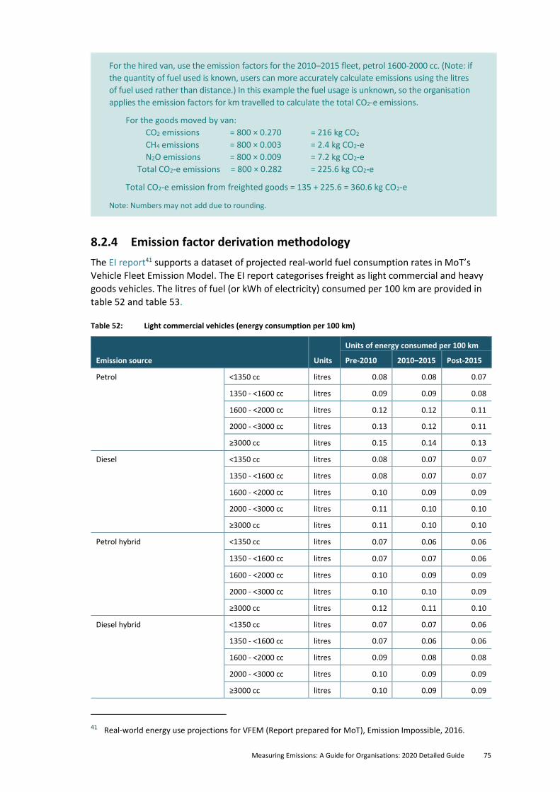
Measuring Emissions: A Guide for Organisations: 2020 Detailed Guide 75
For the hired van, use the emission factors for the 2010–2015 fleet, petrol 1600-2000 cc. (Note: if
the quantity of fuel used is known, users can more accurately calculate emissions using the litres
of fuel used rather than distance.) In this example the fuel usage is unknown, so the organisation
applies the emission factors for km travelled to calculate the total CO2-e emissions.
For the goods moved by van:
CO2 emissions = 800 × 0.270 = 216 kg CO2
CH4 emissions = 800 × 0.003 = 2.4 kg CO2-e
N2O emissions = 800 × 0.009 = 7.2 kg CO2-e
Total CO2-e emissions = 800 × 0.282 = 225.6 kg CO2-e
Total CO2-e emission from freighted goods = 135 + 225.6 = 360.6 kg CO2-e
Note: Numbers may not add due to rounding.
8.2.4 Emission factor derivation methodology
The EI report41 supports a dataset of projected real-world fuel consumption rates in MoT’s
Vehicle Fleet Emission Model. The EI report categorises freight as light commercial and heavy
goods vehicles. The litres of fuel (or kWh of electricity) consumed per 100 km are provided in
table 52 and table 53.
Table 52: Light commercial vehicles (energy consumption per 100 km)
Emission source Units
Units of energy consumed per 100 km
Pre-2010 2010–2015 Post-2015
Petrol <1350 cc litres 0.08 0.08 0.07
1350 - <1600 cc litres 0.09 0.09 0.08
1600 - <2000 cc litres 0.12 0.12 0.11
2000 - <3000 cc litres 0.13 0.12 0.11
≥3000 cc litres 0.15 0.14 0.13
Diesel <1350 cc litres 0.08 0.07 0.07
1350 - <1600 cc litres 0.08 0.07 0.07
1600 - <2000 cc litres 0.10 0.09 0.09
2000 - <3000 cc litres 0.11 0.10 0.10
≥3000 cc litres 0.11 0.10 0.10
Petrol hybrid <1350 cc litres 0.07 0.06 0.06
1350 - <1600 cc litres 0.07 0.07 0.06
1600 - <2000 cc litres 0.10 0.09 0.09
2000 - <3000 cc litres 0.10 0.10 0.09
≥3000 cc litres 0.12 0.11 0.10
Diesel hybrid <1350 cc litres 0.07 0.07 0.06
1350 - <1600 cc litres 0.07 0.06 0.06
1600 - <2000 cc litres 0.09 0.08 0.08
2000 - <3000 cc litres 0.10 0.09 0.09
≥3000 cc litres 0.10 0.09 0.09
41 Real-world energy use projections for VFEM (Report prepared for MoT), Emission Impossible, 2016.
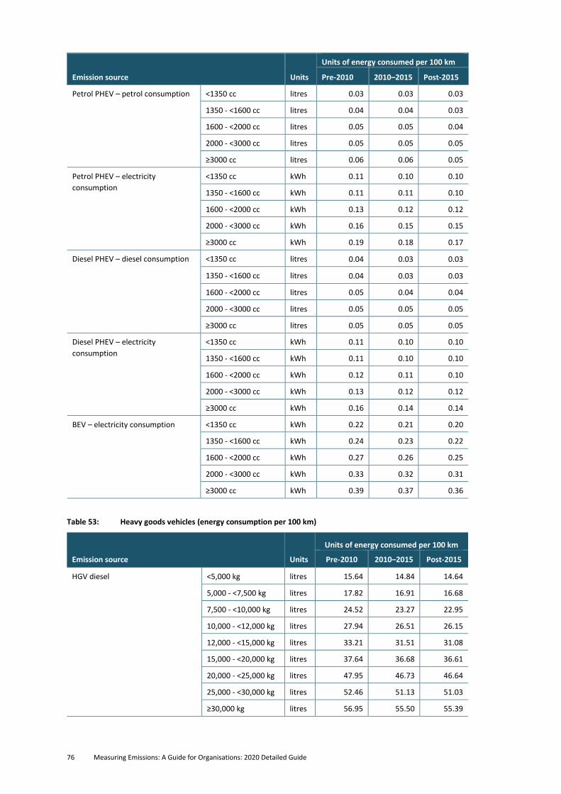
76 Measuring Emissions: A Guide for Organisations: 2020 Detailed Guide
Emission source Units
Units of energy consumed per 100 km
Pre-2010 2010–2015 Post-2015
Petrol PHEV – petrol consumption <1350 cc litres 0.03 0.03 0.03
1350 - <1600 cc litres 0.04 0.04 0.03
1600 - <2000 cc litres 0.05 0.05 0.04
2000 - <3000 cc litres 0.05 0.05 0.05
≥3000 cc litres 0.06 0.06 0.05
Petrol PHEV – electricity
consumption
<1350 cc kWh 0.11 0.10 0.10
1350 - <1600 cc kWh 0.11 0.11 0.10
1600 - <2000 cc kWh 0.13 0.12 0.12
2000 - <3000 cc kWh 0.16 0.15 0.15
≥3000 cc kWh 0.19 0.18 0.17
Diesel PHEV – diesel consumption <1350 cc litres 0.04 0.03 0.03
1350 - <1600 cc litres 0.04 0.03 0.03
1600 - <2000 cc litres 0.05 0.04 0.04
2000 - <3000 cc litres 0.05 0.05 0.05
≥3000 cc litres 0.05 0.05 0.05
Diesel PHEV – electricity
consumption
<1350 cc kWh 0.11 0.10 0.10
1350 - <1600 cc kWh 0.11 0.10 0.10
1600 - <2000 cc kWh 0.12 0.11 0.10
2000 - <3000 cc kWh 0.13 0.12 0.12
≥3000 cc kWh 0.16 0.14 0.14
BEV – electricity consumption <1350 cc kWh 0.22 0.21 0.20
1350 - <1600 cc kWh 0.24 0.23 0.22
1600 - <2000 cc kWh 0.27 0.26 0.25
2000 - <3000 cc kWh 0.33 0.32 0.31
≥3000 cc kWh 0.39 0.37 0.36
Table 53: Heavy goods vehicles (energy consumption per 100 km)
Emission source Units
Units of energy consumed per 100 km
Pre-2010 2010–2015 Post-2015
HGV diesel <5,000 kg litres 15.64 14.84 14.64
5,000 - <7,500 kg litres 17.82 16.91 16.68
7,500 - <10,000 kg litres 24.52 23.27 22.95
10,000 - <12,000 kg litres 27.94 26.51 26.15
12,000 - <15,000 kg litres 33.21 31.51 31.08
15,000 - <20,000 kg litres 37.64 36.68 36.61
20,000 - <25,000 kg litres 47.95 46.73 46.64
25,000 - <30,000 kg litres 52.46 51.13 51.03
≥30,000 kg litres 56.95 55.50 55.39
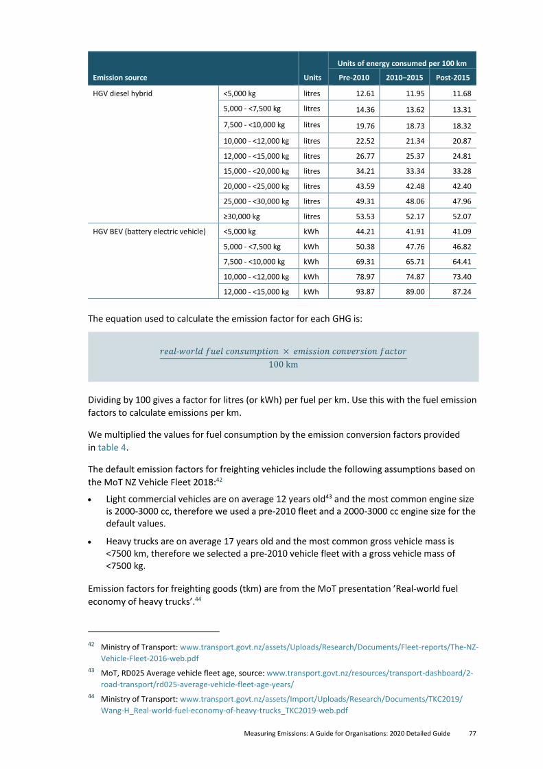
Measuring Emissions: A Guide for Organisations: 2020 Detailed Guide 77
Emission source Units
Units of energy consumed per 100 km
Pre-2010 2010–2015 Post-2015
HGV diesel hybrid <5,000 kg litres 12.61 11.95 11.68
5,000 - <7,500 kg litres 14.36 13.62 13.31
7,500 - <10,000 kg litres 19.76 18.73 18.32
10,000 - <12,000 kg litres 22.52 21.34 20.87
12,000 - <15,000 kg litres 26.77 25.37 24.81
15,000 - <20,000 kg litres 34.21 33.34 33.28
20,000 - <25,000 kg litres 43.59 42.48 42.40
25,000 - <30,000 kg litres 49.31 48.06 47.96
≥30,000 kg litres 53.53 52.17 52.07
HGV BEV (battery electric vehicle) <5,000 kg kWh 44.21 41.91 41.09
5,000 - <7,500 kg kWh 50.38 47.76 46.82
7,500 - <10,000 kg kWh 69.31 65.71 64.41
10,000 - <12,000 kg kWh 78.97 74.87 73.40
12,000 - <15,000 kg kWh 93.87 89.00 87.24
The equation used to calculate the emission factor for each GHG is:
𝑟𝑒𝑎𝑙˗𝑤𝑜𝑟𝑙𝑑 𝑓𝑢𝑒𝑙 𝑐𝑜𝑛𝑠𝑢𝑚𝑝𝑡𝑖𝑜𝑛 × 𝑒𝑚𝑖𝑠𝑠𝑖𝑜𝑛 𝑐𝑜𝑛𝑣𝑒𝑟𝑠𝑖𝑜𝑛 𝑓𝑎𝑐𝑡𝑜𝑟
100 km
Dividing by 100 gives a factor for litres (or kWh) per fuel per km. Use this with the fuel emission
factors to calculate emissions per km.
We multiplied the values for fuel consumption by the emission conversion factors provided
in table 4.
The default emission factors for freighting vehicles include the following assumptions based on
the MoT NZ Vehicle Fleet 2018:42
• Light commercial vehicles are on average 12 years old43 and the most common engine size is 2000-3000 cc, therefore we used a pre-2010 fleet and a 2000-3000 cc engine size for the default values.
• Heavy trucks are on average 17 years old and the most common gross vehicle mass is <7500 km, therefore we selected a pre-2010 vehicle fleet with a gross vehicle mass of <7500 kg.
Emission factors for freighting goods (tkm) are from the MoT presentation ’Real-world fuel
economy of heavy trucks’.44
42 Ministry of Transport: www.transport.govt.nz/assets/Uploads/Research/Documents/Fleet-reports/The-NZ-
Vehicle-Fleet-2016-web.pdf
43 MoT, RD025 Average vehicle fleet age, source: www.transport.govt.nz/resources/transport-dashboard/2-
road-transport/rd025-average-vehicle-fleet-age-years/
44 Ministry of Transport: www.transport.govt.nz/assets/Import/Uploads/Research/Documents/TKC2019/
Wang-H_Real-world-fuel-economy-of-heavy-trucks_TKC2019-web.pdf
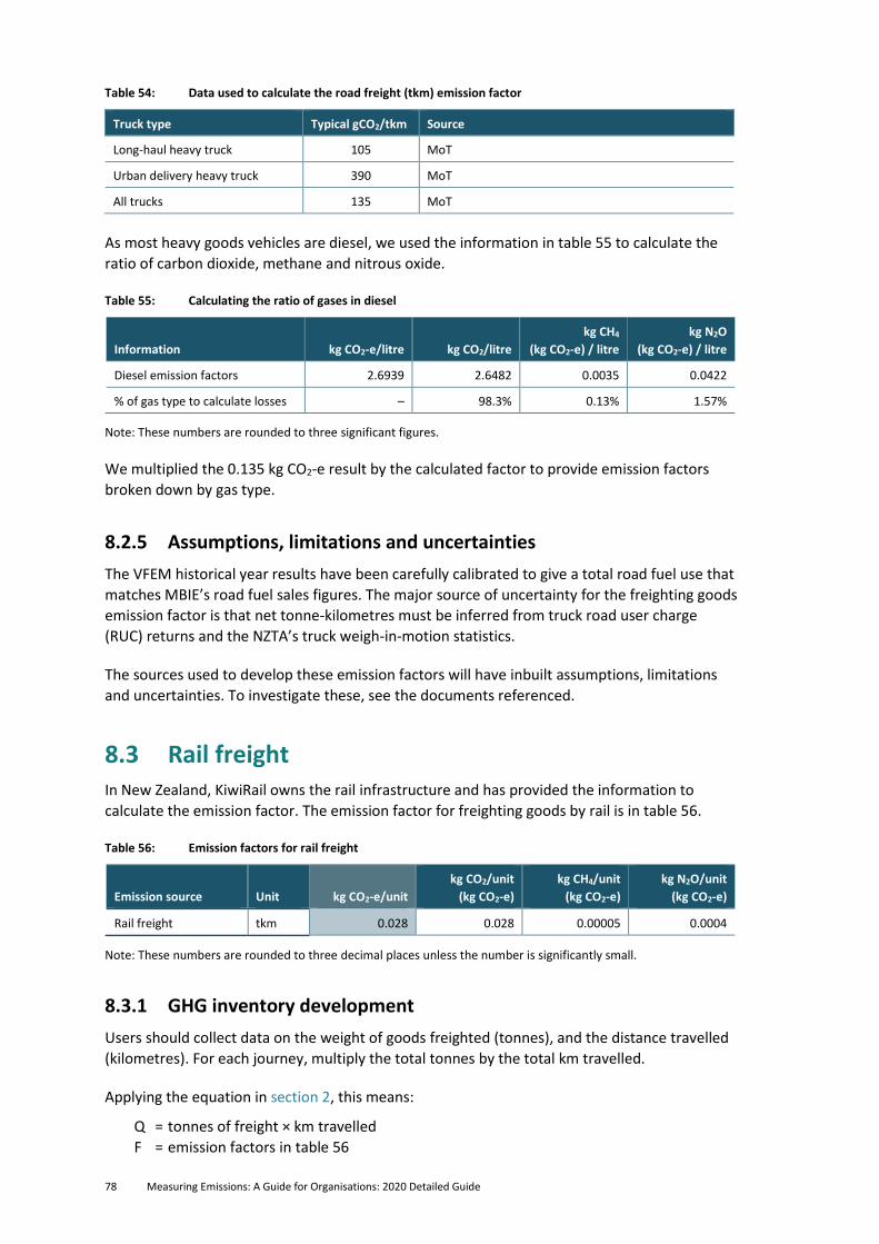
78 Measuring Emissions: A Guide for Organisations: 2020 Detailed Guide
Table 54: Data used to calculate the road freight (tkm) emission factor
Truck type Typical gCO2/tkm Source
Long-haul heavy truck 105 MoT
Urban delivery heavy truck 390 MoT
All trucks 135 MoT
As most heavy goods vehicles are diesel, we used the information in table 55 to calculate the
ratio of carbon dioxide, methane and nitrous oxide.
Table 55: Calculating the ratio of gases in diesel
Information kg CO2-e/litre kg CO2/litre
kg CH4
(kg CO2-e) / litre
kg N2O
(kg CO2-e) / litre
Diesel emission factors 2.6939 2.6482 0.0035 0.0422
% of gas type to calculate losses – 98.3% 0.13% 1.57%
Note: These numbers are rounded to three significant figures.
We multiplied the 0.135 kg CO2-e result by the calculated factor to provide emission factors
broken down by gas type.
8.2.5 Assumptions, limitations and uncertainties
The VFEM historical year results have been carefully calibrated to give a total road fuel use that
matches MBIE’s road fuel sales figures. The major source of uncertainty for the freighting goods
emission factor is that net tonne-kilometres must be inferred from truck road user charge
(RUC) returns and the NZTA’s truck weigh-in-motion statistics.
The sources used to develop these emission factors will have inbuilt assumptions, limitations
and uncertainties. To investigate these, see the documents referenced.
8.3 Rail freight In New Zealand, KiwiRail owns the rail infrastructure and has provided the information to
calculate the emission factor. The emission factor for freighting goods by rail is in table 56.
Table 56: Emission factors for rail freight
Emission source Unit kg CO2-e/unit
kg CO2/unit
(kg CO2-e)
kg CH4/unit
(kg CO2-e)
kg N2O/unit
(kg CO2-e)
Rail freight tkm 0.028 0.028 0.00005 0.0004
Note: These numbers are rounded to three decimal places unless the number is significantly small.
8.3.1 GHG inventory development
Users should collect data on the weight of goods freighted (tonnes), and the distance travelled
(kilometres). For each journey, multiply the total tonnes by the total km travelled.
Applying the equation in section 2, this means:
Q = tonnes of freight × km travelled
F = emission factors in table 56
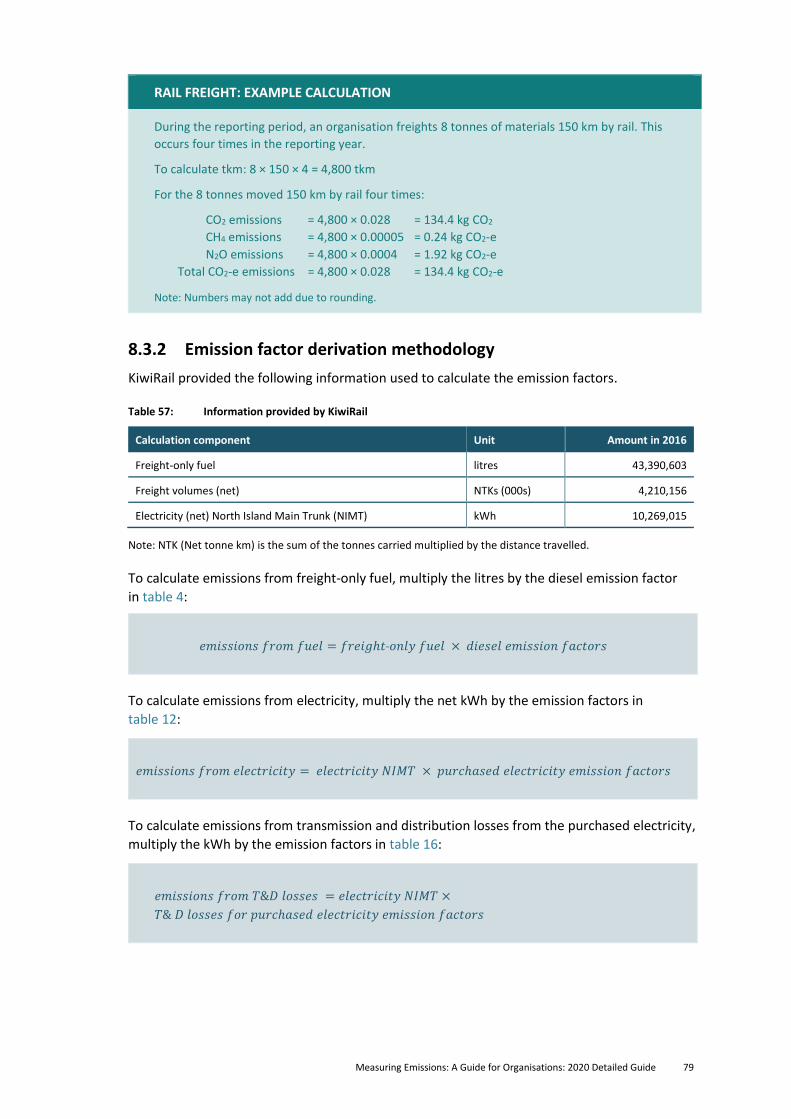
Measuring Emissions: A Guide for Organisations: 2020 Detailed Guide 79
RAIL FREIGHT: EXAMPLE CALCULATION
During the reporting period, an organisation freights 8 tonnes of materials 150 km by rail. This
occurs four times in the reporting year.
To calculate tkm: 8 × 150 × 4 = 4,800 tkm
For the 8 tonnes moved 150 km by rail four times:
CO2 emissions = 4,800 × 0.028 = 134.4 kg CO2
CH4 emissions = 4,800 × 0.00005 = 0.24 kg CO2-e
N2O emissions = 4,800 × 0.0004 = 1.92 kg CO2-e
Total CO2-e emissions = 4,800 × 0.028 = 134.4 kg CO2-e
Note: Numbers may not add due to rounding.
8.3.2 Emission factor derivation methodology
KiwiRail provided the following information used to calculate the emission factors.
Table 57: Information provided by KiwiRail
Calculation component Unit Amount in 2016
Freight-only fuel litres 43,390,603
Freight volumes (net) NTKs (000s) 4,210,156
Electricity (net) North Island Main Trunk (NIMT) kWh 10,269,015
Note: NTK (Net tonne km) is the sum of the tonnes carried multiplied by the distance travelled.
To calculate emissions from freight-only fuel, multiply the litres by the diesel emission factor
in table 4:
𝑒𝑚𝑖𝑠𝑠𝑖𝑜𝑛𝑠 𝑓𝑟𝑜𝑚 𝑓𝑢𝑒𝑙 = 𝑓𝑟𝑒𝑖𝑔ℎ𝑡˗𝑜𝑛𝑙𝑦 𝑓𝑢𝑒𝑙 × 𝑑𝑖𝑒𝑠𝑒𝑙 𝑒𝑚𝑖𝑠𝑠𝑖𝑜𝑛 𝑓𝑎𝑐𝑡𝑜𝑟𝑠
To calculate emissions from electricity, multiply the net kWh by the emission factors in
table 12:
𝑒𝑚𝑖𝑠𝑠𝑖𝑜𝑛𝑠 𝑓𝑟𝑜𝑚 𝑒𝑙𝑒𝑐𝑡𝑟𝑖𝑐𝑖𝑡𝑦 = 𝑒𝑙𝑒𝑐𝑡𝑟𝑖𝑐𝑖𝑡𝑦 𝑁𝐼𝑀𝑇 × 𝑝𝑢𝑟𝑐ℎ𝑎𝑠𝑒𝑑 𝑒𝑙𝑒𝑐𝑡𝑟𝑖𝑐𝑖𝑡𝑦 𝑒𝑚𝑖𝑠𝑠𝑖𝑜𝑛 𝑓𝑎𝑐𝑡𝑜𝑟𝑠
To calculate emissions from transmission and distribution losses from the purchased electricity,
multiply the kWh by the emission factors in table 16:
𝑒𝑚𝑖𝑠𝑠𝑖𝑜𝑛𝑠 𝑓𝑟𝑜𝑚 𝑇&𝐷 𝑙𝑜𝑠𝑠𝑒𝑠 = 𝑒𝑙𝑒𝑐𝑡𝑟𝑖𝑐𝑖𝑡𝑦 𝑁𝐼𝑀𝑇 ×
𝑇& 𝐷 𝑙𝑜𝑠𝑠𝑒𝑠 𝑓𝑜𝑟 𝑝𝑢𝑟𝑐ℎ𝑎𝑠𝑒𝑑 𝑒𝑙𝑒𝑐𝑡𝑟𝑖𝑐𝑖𝑡𝑦 𝑒𝑚𝑖𝑠𝑠𝑖𝑜𝑛 𝑓𝑎𝑐𝑡𝑜𝑟𝑠
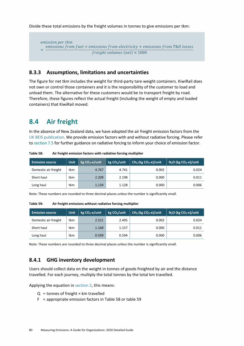
80 Measuring Emissions: A Guide for Organisations: 2020 Detailed Guide
Divide these total emissions by the freight volumes in tonnes to give emissions per tkm:
𝑒𝑚𝑖𝑠𝑠𝑖𝑜𝑛 𝑝𝑒𝑟 𝑡𝑘𝑚
= 𝑒𝑚𝑖𝑠𝑠𝑖𝑜𝑛𝑠 𝑓𝑟𝑜𝑚 𝑓𝑢𝑒𝑙 + 𝑒𝑚𝑖𝑠𝑠𝑖𝑜𝑛𝑠 𝑓𝑟𝑜𝑚 𝑒𝑙𝑒𝑐𝑡𝑟𝑖𝑐𝑖𝑡𝑦 + 𝑒𝑚𝑖𝑠𝑠𝑖𝑜𝑛𝑠 𝑓𝑟𝑜𝑚 𝑇&𝐷 𝑙𝑜𝑠𝑠𝑒𝑠
𝑓𝑟𝑒𝑖𝑔ℎ𝑡 𝑣𝑜𝑙𝑢𝑚𝑒𝑠 (𝑛𝑒𝑡) × 1000
8.3.3 Assumptions, limitations and uncertainties
The figure for net tkm includes the weight for third-party tare weight containers. KiwiRail does
not own or control those containers and it is the responsibility of the customer to load and
unload them. The alternative for these customers would be to transport freight by road.
Therefore, these figures reflect the actual freight (including the weight of empty and loaded
containers) that KiwiRail moved.
8.4 Air freight In the absence of New Zealand data, we have adopted the air freight emission factors from the
UK BEIS publication. We provide emission factors with and without radiative forcing. Please refer
to section 7.5 for further guidance on radiative forcing to inform your choice of emission factor.
Table 58: Air freight emission factors with radiative forcing multiplier
Emission source Unit kg CO2-e/unit kg CO2/unit CH4 (kg CO2-e)/unit N2O (kg CO2-e)/unit
Domestic air freight tkm 4.767 4.741 0.002 0.024
Short haul tkm 2.209 2.198 0.000 0.011
Long haul tkm 1.134 1.128 0.000 0.006
Note: These numbers are rounded to three decimal places unless the number is significantly small.
Table 59: Air freight emissions without radiative forcing multiplier
Emission source Unit kg CO2-e/unit kg CO2/unit CH4 (kg CO2-e)/unit N2O (kg CO2-e)/unit
Domestic air freight tkm 2.521 2.495 0.002 0.024
Short haul tkm 1.168 1.157 0.000 0.011
Long haul tkm 0.599 0.594 0.000 0.006
Note: These numbers are rounded to three decimal places unless the number is significantly small.
8.4.1 GHG inventory development
Users should collect data on the weight in tonnes of goods freighted by air and the distance
travelled. For each journey, multiply the total tonnes by the total km travelled.
Applying the equation in section 2, this means:
Q = tonnes of freight × km travelled
F = appropriate emission factors in Table 58 or table 59
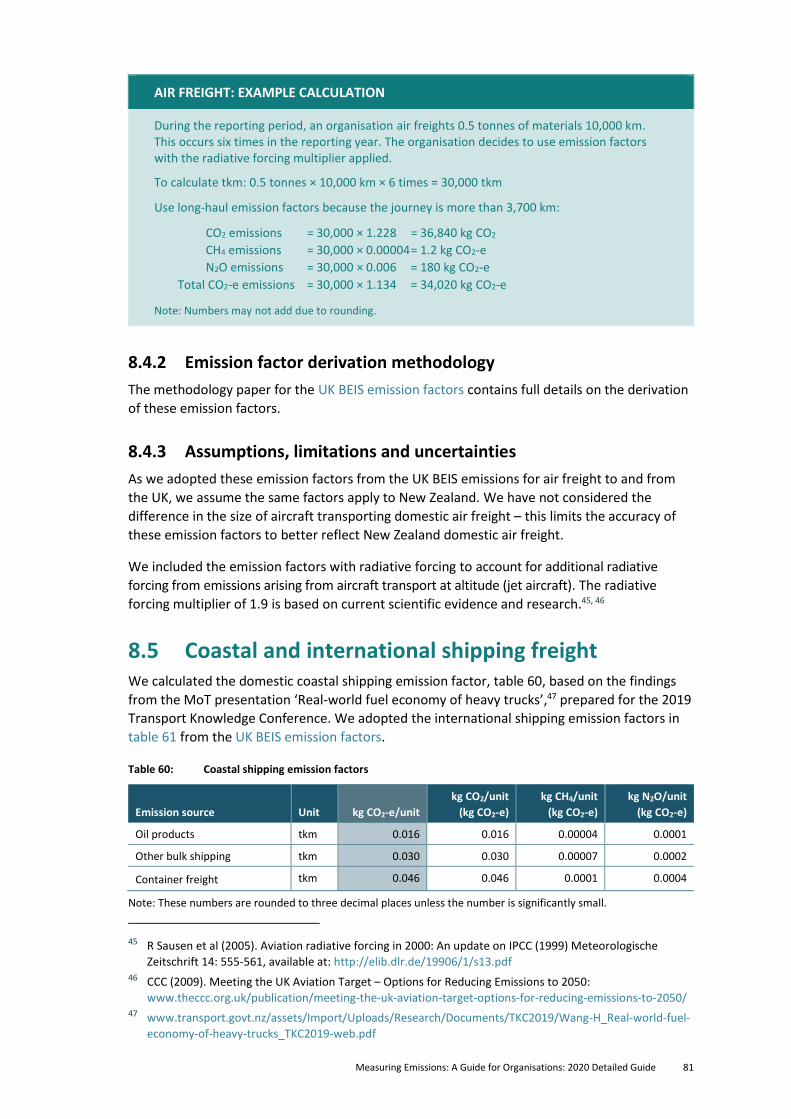
Measuring Emissions: A Guide for Organisations: 2020 Detailed Guide 81
AIR FREIGHT: EXAMPLE CALCULATION
During the reporting period, an organisation air freights 0.5 tonnes of materials 10,000 km. This occurs six times in the reporting year. The organisation decides to use emission factors with the radiative forcing multiplier applied.
To calculate tkm: 0.5 tonnes × 10,000 km × 6 times = 30,000 tkm
Use long-haul emission factors because the journey is more than 3,700 km:
CO2 emissions = 30,000 × 1.228 = 36,840 kg CO2
CH4 emissions = 30,000 × 0.00004 = 1.2 kg CO2-e
N2O emissions = 30,000 × 0.006 = 180 kg CO2-e
Total CO2-e emissions = 30,000 × 1.134 = 34,020 kg CO2-e
Note: Numbers may not add due to rounding.
8.4.2 Emission factor derivation methodology
The methodology paper for the UK BEIS emission factors contains full details on the derivation
of these emission factors.
8.4.3 Assumptions, limitations and uncertainties
As we adopted these emission factors from the UK BEIS emissions for air freight to and from
the UK, we assume the same factors apply to New Zealand. We have not considered the
difference in the size of aircraft transporting domestic air freight – this limits the accuracy of
these emission factors to better reflect New Zealand domestic air freight.
We included the emission factors with radiative forcing to account for additional radiative
forcing from emissions arising from aircraft transport at altitude (jet aircraft). The radiative
forcing multiplier of 1.9 is based on current scientific evidence and research.45, 46
8.5 Coastal and international shipping freight We calculated the domestic coastal shipping emission factor, table 60, based on the findings
from the MoT presentation ‘Real-world fuel economy of heavy trucks’,47 prepared for the 2019
Transport Knowledge Conference. We adopted the international shipping emission factors in
table 61 from the UK BEIS emission factors.
Table 60: Coastal shipping emission factors
Emission source Unit kg CO2-e/unit
kg CO2/unit
(kg CO2-e)
kg CH4/unit
(kg CO2-e)
kg N2O/unit
(kg CO2-e)
Oil products tkm 0.016 0.016 0.00004 0.0001
Other bulk shipping tkm 0.030 0.030 0.00007 0.0002
Container freight tkm 0.046 0.046 0.0001 0.0004
Note: These numbers are rounded to three decimal places unless the number is significantly small.
45 R Sausen et al (2005). Aviation radiative forcing in 2000: An update on IPCC (1999) Meteorologische
Zeitschrift 14: 555-561, available at: http://elib.dlr.de/19906/1/s13.pdf 46 CCC (2009). Meeting the UK Aviation Target – Options for Reducing Emissions to 2050:
www.theccc.org.uk/publication/meeting-the-uk-aviation-target-options-for-reducing-emissions-to-2050/ 47 www.transport.govt.nz/assets/Import/Uploads/Research/Documents/TKC2019/Wang-H_Real-world-fuel-
economy-of-heavy-trucks_TKC2019-web.pdf
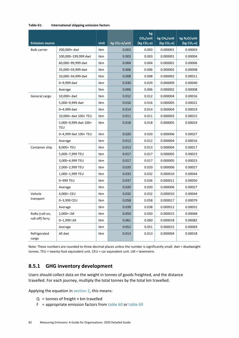
82 Measuring Emissions: A Guide for Organisations: 2020 Detailed Guide
Table 61: International shipping emission factors
Emission source Unit kg CO2-e/unit
kg
CO2/unit
(kg CO2-e)
kg CH4/unit
(kg CO2-e)
kg N2O/unit
(kg CO2-e)
Bulk carrier 200,000+ dwt tkm 0.003 0.003 0.000001 0.00003
100,000–199,999 dwt tkm 0.003 0.003 0.000001 0.00004
60,000–99,999 dwt tkm 0.004 0.004 0.000001 0.00006
35,000–59,999 dwt tkm 0.006 0.006 0.000002 0.00008
10,000–34,999 dwt tkm 0.008 0.008 0.000002 0.00011
0–9,999 dwt tkm 0.030 0.029 0.000009 0.00040
Average tkm 0.006 0.006 0.000002 0.00008
General cargo 10,000+ dwt tkm 0.012 0.012 0.000004 0.00016
5,000–9,999 dwt tkm 0.016 0.016 0.000005 0.00022
0–4,999 dwt tkm 0.014 0.014 0.000004 0.00019
10,000+ dwt 100+ TEU tkm 0.011 0.011 0.000003 0.00015
5,000–9,999 dwt 100+
TEU
tkm 0.018 0.018 0.000005 0.00024
0–4,999 dwt 100+ TEU tkm 0.020 0.020 0.000006 0.00027
Average tkm 0.012 0.012 0.000004 0.00016
Container ship 8,000+ TEU tkm 0.013 0.013 0.000004 0.00017
5,000–7,999 TEU tkm 0.017 0.017 0.000005 0.00023
3,000–4,999 TEU tkm 0.017 0.017 0.000005 0.00023
2,000–2,999 TEU tkm 0.020 0.020 0.000006 0.00027
1,000–1,999 TEU tkm 0.033 0.032 0.000010 0.00044
0–999 TEU tkm 0.037 0.036 0.000011 0.00050
Average tkm 0.020 0.020 0.000006 0.00027
Vehicle
transport
4,000+ CEU tkm 0.032 0.032 0.000010 0.00044
0–3,999 CEU tkm 0.058 0.058 0.000017 0.00079
Average tkm 0.039 0.038 0.000012 0.00052
RoRo (roll-on,
roll-off) ferry
2,000+ LM tkm 0.050 0.050 0.000015 0.00068
0–1,999 LM tkm 0.061 0.060 0.000018 0.00082
Average tkm 0.052 0.051 0.000015 0.00069
Refrigerated
cargo
All dwt tkm 0.013 0.013 0.000004 0.00018
Note: These numbers are rounded to three decimal places unless the number is significantly small. dwt = deadweight
tonnes. TEU = twenty-foot equivalent unit. CEU = car equivalent unit. LM = lanemetre.
8.5.1 GHG inventory development
Users should collect data on the weight in tonnes of goods freighted, and the distance
travelled. For each journey, multiply the total tonnes by the total km travelled.
Applying the equation in section 2, this means:
Q = tonnes of freight × km travelled
F = appropriate emission factors from table 60 or table 69
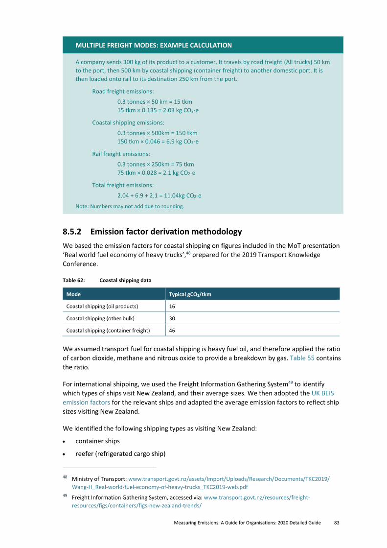
Measuring Emissions: A Guide for Organisations: 2020 Detailed Guide 83
MULTIPLE FREIGHT MODES: EXAMPLE CALCULATION
A company sends 300 kg of its product to a customer. It travels by road freight (All trucks) 50 km
to the port, then 500 km by coastal shipping (container freight) to another domestic port. It is
then loaded onto rail to its destination 250 km from the port.
Road freight emissions:
0.3 tonnes × 50 km = 15 tkm
15 tkm × 0.135 = 2.03 kg CO2-e
Coastal shipping emissions:
0.3 tonnes × 500km = 150 tkm
150 tkm × 0.046 = 6.9 kg CO2-e
Rail freight emissions:
0.3 tonnes × 250km = 75 tkm
75 tkm × 0.028 = 2.1 kg CO2-e
Total freight emissions:
2.04 + 6.9 + 2.1 = 11.04kg CO2-e
Note: Numbers may not add due to rounding.
8.5.2 Emission factor derivation methodology
We based the emission factors for coastal shipping on figures included in the MoT presentation
‘Real world fuel economy of heavy trucks’,48 prepared for the 2019 Transport Knowledge
Conference.
Table 62: Coastal shipping data
Mode Typical gCO2/tkm
Coastal shipping (oil products) 16
Coastal shipping (other bulk) 30
Coastal shipping (container freight) 46
We assumed transport fuel for coastal shipping is heavy fuel oil, and therefore applied the ratio
of carbon dioxide, methane and nitrous oxide to provide a breakdown by gas. Table 55 contains
the ratio.
For international shipping, we used the Freight Information Gathering System49 to identify
which types of ships visit New Zealand, and their average sizes. We then adopted the UK BEIS
emission factors for the relevant ships and adapted the average emission factors to reflect ship
sizes visiting New Zealand.
We identified the following shipping types as visiting New Zealand:
• container ships
• reefer (refrigerated cargo ship)
48 Ministry of Transport: www.transport.govt.nz/assets/Import/Uploads/Research/Documents/TKC2019/
Wang-H_Real-world-fuel-economy-of-heavy-trucks_TKC2019-web.pdf
49 Freight Information Gathering System, accessed via: www.transport.govt.nz/resources/freight-
resources/figs/containers/figs-new-zealand-trends/
84 Measuring Emissions: A Guide for Organisations: 2020 Detailed Guide
• bulk carrier
• RoRo (roll-on, roll-off)
• oil/gas tanker
• vehicle carrier
• general cargo.
We used MoT’s Freight Information Gathering System (FIGS)50 to find out the average sizes of
ships visiting New Zealand. Ships are measured in deadweight tonnes (dwt), twenty-foot
equivalent unit (TEU), car equivalent unit (CEU) or lanemetre (LM).
• Bulk carrier is 36,900 dwt and therefore in the 35,000–59,999 dwt category.
• General cargo is 15,800 dwt and therefore in the 10,000+ dwt category.
• Container ship is 2923 TEU and therefore in the 2000–2999 TEU category.
• Vehicle carrier (transport) is unknown and therefore the same as the UK average.
• RoRo ferry is unknown and therefore the same as the UK average.
• As there is only one emission factor for all refrigerated cargo an average was not necessary.
Emission factors for these have been adopted from the UK BEIS 2020 Guidance.51 Please refer
to that document for details on the methodology.
8.5.3 Assumptions, limitations and uncertainties
We assumed the New Zealand coastal shipping fleet is similar to that in the STREAM Freight
Handbook. These figures have a high degree of uncertainty as they are based on international
data for costal shipping.
We carried over the assumptions for the international shipping emission factors from the UK
BEIS 2020 emission factors.
50 Freight Information Gathering System, overseas ships, accessed via:
www.transport.govt.nz/resources/freight-resources/figs/overseas-ship-visits/
51 UK BEIS 2020 Guidance, accessed via: https://www.gov.uk/government/publications/greenhouse-gas-
reporting-conversion-factors-2020
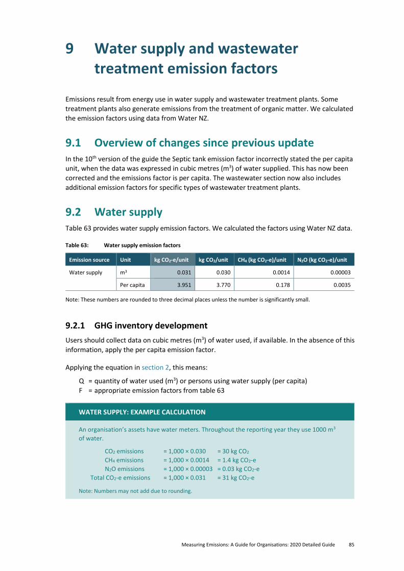
Measuring Emissions: A Guide for Organisations: 2020 Detailed Guide 85
9 Water supply and wastewater treatment emission factors
Emissions result from energy use in water supply and wastewater treatment plants. Some
treatment plants also generate emissions from the treatment of organic matter. We calculated
the emission factors using data from Water NZ.
9.1 Overview of changes since previous update In the 10th version of the guide the Septic tank emission factor incorrectly stated the per capita
unit, when the data was expressed in cubic metres (m3) of water supplied. This has now been
corrected and the emissions factor is per capita. The wastewater section now also includes
additional emission factors for specific types of wastewater treatment plants.
9.2 Water supply Table 63 provides water supply emission factors. We calculated the factors using Water NZ data.
Table 63: Water supply emission factors
Emission source Unit kg CO2-e/unit kg CO2/unit CH4 (kg CO2-e)/unit N2O (kg CO2-e)/unit
Water supply m3 0.031 0.030 0.0014 0.00003
Per capita 3.951 3.770 0.178 0.0035
Note: These numbers are rounded to three decimal places unless the number is significantly small.
9.2.1 GHG inventory development
Users should collect data on cubic metres (m3) of water used, if available. In the absence of this
information, apply the per capita emission factor.
Applying the equation in section 2, this means:
Q = quantity of water used (m3) or persons using water supply (per capita)
F = appropriate emission factors from table 63
WATER SUPPLY: EXAMPLE CALCULATION
An organisation’s assets have water meters. Throughout the reporting year they use 1000 m3
of water.
CO2 emissions = 1,000 × 0.030 = 30 kg CO2
CH4 emissions = 1,000 × 0.0014 = 1.4 kg CO2-e
N2O emissions = 1,000 × 0.00003 = 0.03 kg CO2-e
Total CO2-e emissions = 1,000 × 0.031 = 31 kg CO2-e
Note: Numbers may not add due to rounding.
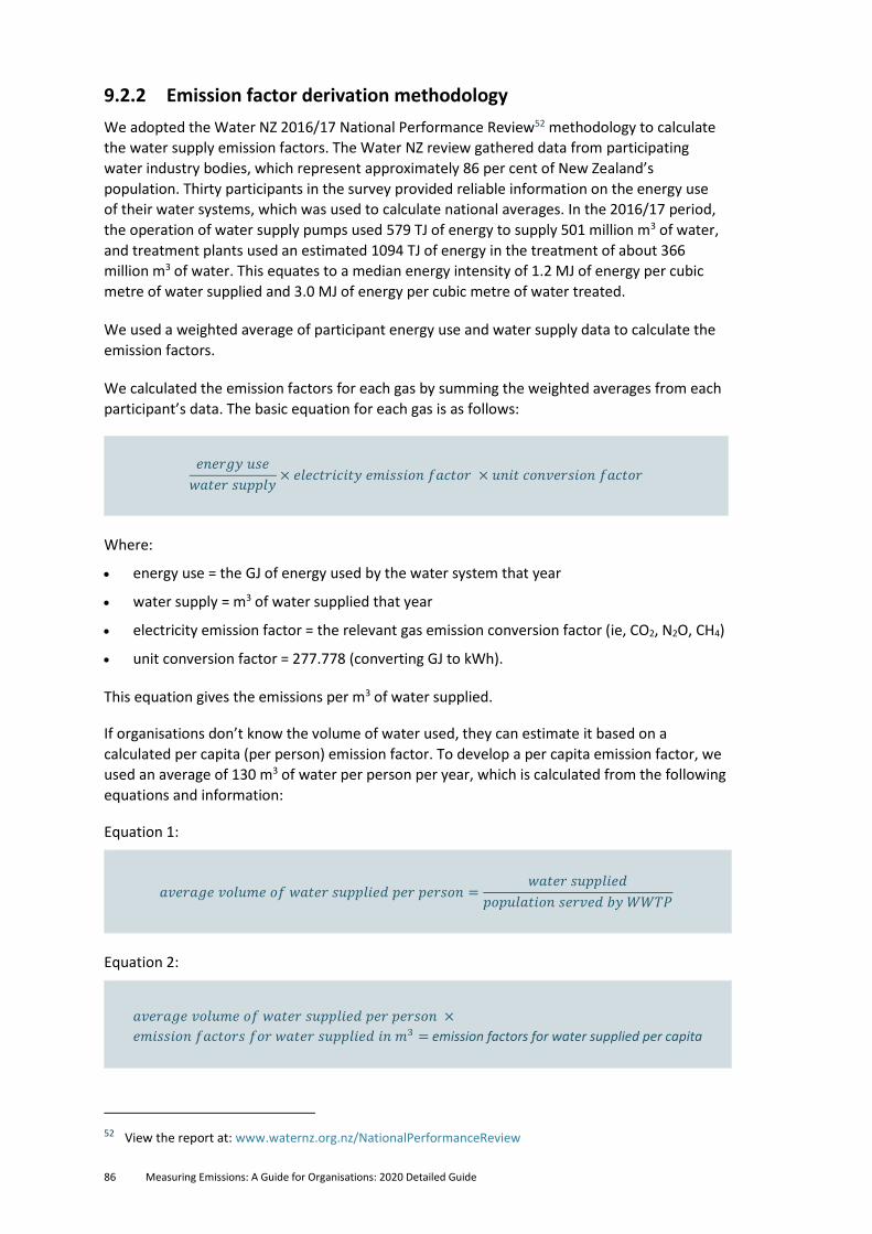
86 Measuring Emissions: A Guide for Organisations: 2020 Detailed Guide
9.2.2 Emission factor derivation methodology
We adopted the Water NZ 2016/17 National Performance Review52 methodology to calculate
the water supply emission factors. The Water NZ review gathered data from participating
water industry bodies, which represent approximately 86 per cent of New Zealand’s
population. Thirty participants in the survey provided reliable information on the energy use
of their water systems, which was used to calculate national averages. In the 2016/17 period,
the operation of water supply pumps used 579 TJ of energy to supply 501 million m3 of water,
and treatment plants used an estimated 1094 TJ of energy in the treatment of about 366
million m3 of water. This equates to a median energy intensity of 1.2 MJ of energy per cubic
metre of water supplied and 3.0 MJ of energy per cubic metre of water treated.
We used a weighted average of participant energy use and water supply data to calculate the
emission factors.
We calculated the emission factors for each gas by summing the weighted averages from each
participant’s data. The basic equation for each gas is as follows:
𝑒𝑛𝑒𝑟𝑔𝑦 𝑢𝑠𝑒
𝑤𝑎𝑡𝑒𝑟 𝑠𝑢𝑝𝑝𝑙𝑦× 𝑒𝑙𝑒𝑐𝑡𝑟𝑖𝑐𝑖𝑡𝑦 𝑒𝑚𝑖𝑠𝑠𝑖𝑜𝑛 𝑓𝑎𝑐𝑡𝑜𝑟 × 𝑢𝑛𝑖𝑡 𝑐𝑜𝑛𝑣𝑒𝑟𝑠𝑖𝑜𝑛 𝑓𝑎𝑐𝑡𝑜𝑟
Where:
• energy use = the GJ of energy used by the water system that year
• water supply = m3 of water supplied that year
• electricity emission factor = the relevant gas emission conversion factor (ie, CO2, N2O, CH4)
• unit conversion factor = 277.778 (converting GJ to kWh).
This equation gives the emissions per m3 of water supplied.
If organisations don’t know the volume of water used, they can estimate it based on a
calculated per capita (per person) emission factor. To develop a per capita emission factor, we
used an average of 130 m3 of water per person per year, which is calculated from the following
equations and information:
Equation 1:
𝑎𝑣𝑒𝑟𝑎𝑔𝑒 𝑣𝑜𝑙𝑢𝑚𝑒 𝑜𝑓 𝑤𝑎𝑡𝑒𝑟 𝑠𝑢𝑝𝑝𝑙𝑖𝑒𝑑 𝑝𝑒𝑟 𝑝𝑒𝑟𝑠𝑜𝑛 =𝑤𝑎𝑡𝑒𝑟 𝑠𝑢𝑝𝑝𝑙𝑖𝑒𝑑
𝑝𝑜𝑝𝑢𝑙𝑎𝑡𝑖𝑜𝑛 𝑠𝑒𝑟𝑣𝑒𝑑 𝑏𝑦 𝑊𝑊𝑇𝑃
Equation 2:
𝑎𝑣𝑒𝑟𝑎𝑔𝑒 𝑣𝑜𝑙𝑢𝑚𝑒 𝑜𝑓 𝑤𝑎𝑡𝑒𝑟 𝑠𝑢𝑝𝑝𝑙𝑖𝑒𝑑 𝑝𝑒𝑟 𝑝𝑒𝑟𝑠𝑜𝑛 ×
𝑒𝑚𝑖𝑠𝑠𝑖𝑜𝑛 𝑓𝑎𝑐𝑡𝑜𝑟𝑠 𝑓𝑜𝑟 𝑤𝑎𝑡𝑒𝑟 𝑠𝑢𝑝𝑝𝑙𝑖𝑒𝑑 𝑖𝑛 𝑚3 = emission factors for water supplied per capita
52 View the report at: www.waternz.org.nz/NationalPerformanceReview
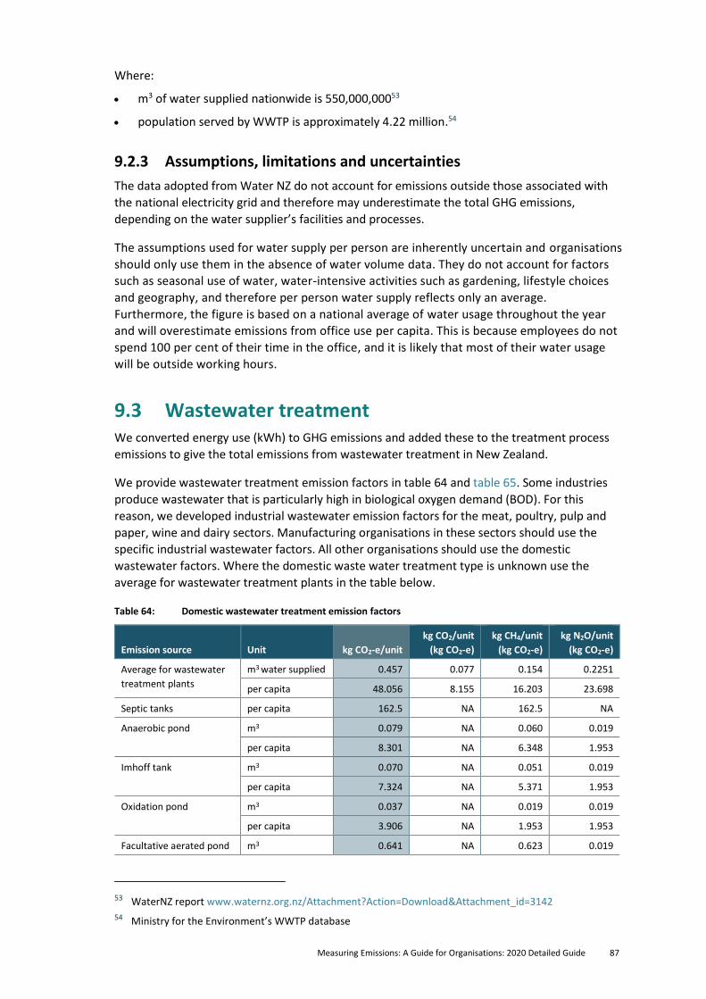
Measuring Emissions: A Guide for Organisations: 2020 Detailed Guide 87
Where:
• m3 of water supplied nationwide is 550,000,00053
• population served by WWTP is approximately 4.22 million.54
9.2.3 Assumptions, limitations and uncertainties
The data adopted from Water NZ do not account for emissions outside those associated with
the national electricity grid and therefore may underestimate the total GHG emissions,
depending on the water supplier’s facilities and processes.
The assumptions used for water supply per person are inherently uncertain and organisations
should only use them in the absence of water volume data. They do not account for factors
such as seasonal use of water, water-intensive activities such as gardening, lifestyle choices
and geography, and therefore per person water supply reflects only an average.
Furthermore, the figure is based on a national average of water usage throughout the year
and will overestimate emissions from office use per capita. This is because employees do not
spend 100 per cent of their time in the office, and it is likely that most of their water usage
will be outside working hours.
9.3 Wastewater treatment We converted energy use (kWh) to GHG emissions and added these to the treatment process
emissions to give the total emissions from wastewater treatment in New Zealand.
We provide wastewater treatment emission factors in table 64 and table 65. Some industries
produce wastewater that is particularly high in biological oxygen demand (BOD). For this
reason, we developed industrial wastewater emission factors for the meat, poultry, pulp and
paper, wine and dairy sectors. Manufacturing organisations in these sectors should use the
specific industrial wastewater factors. All other organisations should use the domestic
wastewater factors. Where the domestic waste water treatment type is unknown use the
average for wastewater treatment plants in the table below.
Table 64: Domestic wastewater treatment emission factors
Emission source Unit kg CO2-e/unit
kg CO2/unit
(kg CO2-e)
kg CH4/unit
(kg CO2-e)
kg N2O/unit
(kg CO2-e)
Average for wastewater
treatment plants
m3 water supplied 0.457 0.077 0.154 0.2251
per capita 48.056 8.155 16.203 23.698
Septic tanks per capita 162.5 NA 162.5 NA
Anaerobic pond m3 0.079 NA 0.060 0.019
per capita 8.301 NA 6.348 1.953
Imhoff tank m3 0.070 NA 0.051 0.019
per capita 7.324 NA 5.371 1.953
Oxidation pond m3 0.037 NA 0.019 0.019
per capita 3.906 NA 1.953 1.953
Facultative aerated pond m3 0.641 NA 0.623 0.019
53 WaterNZ report www.waternz.org.nz/Attachment?Action=Download&Attachment_id=3142
54 Ministry for the Environment’s WWTP database
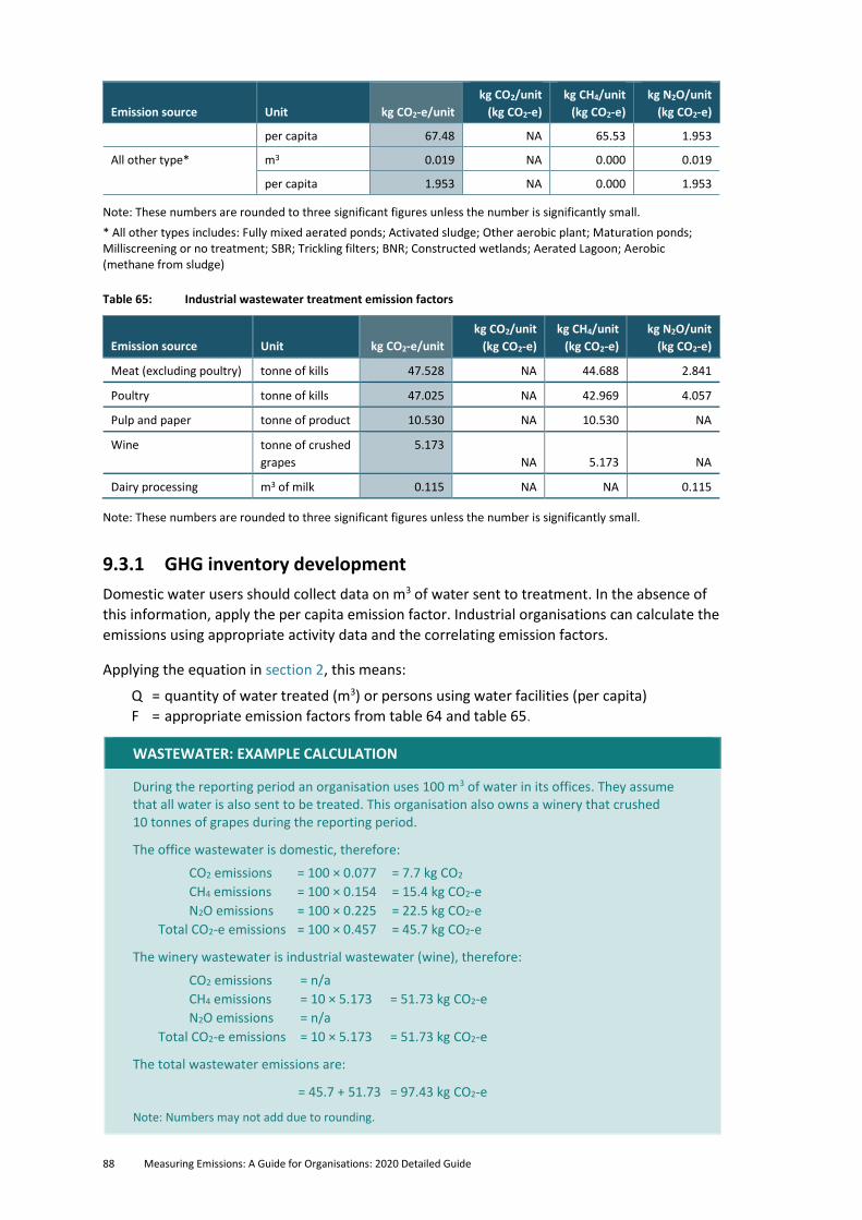
88 Measuring Emissions: A Guide for Organisations: 2020 Detailed Guide
Emission source Unit kg CO2-e/unit
kg CO2/unit
(kg CO2-e)
kg CH4/unit
(kg CO2-e)
kg N2O/unit
(kg CO2-e)
per capita 67.48 NA 65.53 1.953
All other type* m3 0.019 NA 0.000 0.019
per capita 1.953 NA 0.000 1.953
Note: These numbers are rounded to three significant figures unless the number is significantly small.
* All other types includes: Fully mixed aerated ponds; Activated sludge; Other aerobic plant; Maturation ponds; Milliscreening or no treatment; SBR; Trickling filters; BNR; Constructed wetlands; Aerated Lagoon; Aerobic (methane from sludge)
Table 65: Industrial wastewater treatment emission factors
Emission source Unit kg CO2-e/unit
kg CO2/unit
(kg CO2-e)
kg CH4/unit
(kg CO2-e)
kg N2O/unit
(kg CO2-e)
Meat (excluding poultry) tonne of kills 47.528 NA 44.688 2.841
Poultry tonne of kills 47.025 NA 42.969 4.057
Pulp and paper tonne of product 10.530 NA 10.530 NA
Wine tonne of crushed
grapes
5.173
NA 5.173 NA
Dairy processing m3 of milk 0.115 NA NA 0.115
Note: These numbers are rounded to three significant figures unless the number is significantly small.
9.3.1 GHG inventory development
Domestic water users should collect data on m3 of water sent to treatment. In the absence of
this information, apply the per capita emission factor. Industrial organisations can calculate the
emissions using appropriate activity data and the correlating emission factors.
Applying the equation in section 2, this means:
Q = quantity of water treated (m3) or persons using water facilities (per capita)
F = appropriate emission factors from table 64 and table 65.
WASTEWATER: EXAMPLE CALCULATION
During the reporting period an organisation uses 100 m3 of water in its offices. They assume that all water is also sent to be treated. This organisation also owns a winery that crushed 10 tonnes of grapes during the reporting period.
The office wastewater is domestic, therefore:
CO2 emissions = 100 × 0.077 = 7.7 kg CO2
CH4 emissions = 100 × 0.154 = 15.4 kg CO2-e
N2O emissions = 100 × 0.225 = 22.5 kg CO2-e
Total CO2-e emissions = 100 × 0.457 = 45.7 kg CO2-e
The winery wastewater is industrial wastewater (wine), therefore:
CO2 emissions = n/a
CH4 emissions = 10 × 5.173 = 51.73 kg CO2-e
N2O emissions = n/a
Total CO2-e emissions = 10 × 5.173 = 51.73 kg CO2-e
The total wastewater emissions are:
= 45.7 + 51.73 = 97.43 kg CO2-e
Note: Numbers may not add due to rounding.
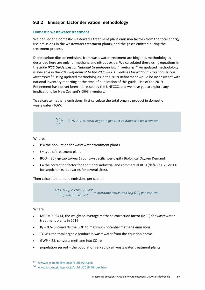
Measuring Emissions: A Guide for Organisations: 2020 Detailed Guide 89
9.3.2 Emission factor derivation methodology
Domestic wastewater treatment
We derived the domestic wastewater treatment plant emission factors from the total energy
use emissions in the wastewater treatment plants, and the gases emitted during the
treatment process.
Direct carbon dioxide emissions from wastewater treatment are biogenic, methodologies
described here are only for methane and nitrous oxide. We calculated these using equations in
the 2006 IPCC Guidelines for National Greenhouse Gas Inventories.55 An updated methodology
is available in the 2019 Refinement to the 2006 IPCC Guidelines for National Greenhouse Gas
Inventories.56 Using updated methodologies in the 2019 Refinement would be inconsistent with
national inventory reporting at the time of publication of this guide. Use of the 2019
Refinement has not yet been addressed by the UNFCCC, and we have yet to explore any
implications for New Zealand’s GHG inventory.
To calculate methane emissions, first calculate the total organic product in domestic
wastewater (TOW):
∑ 𝑃𝑖 × 𝐵𝑂𝐷 × 𝐼
𝑖
= 𝑡𝑜𝑡𝑎𝑙 𝑜𝑟𝑔𝑎𝑛𝑖𝑐 𝑝𝑟𝑜𝑑𝑢𝑐𝑡 𝑖𝑛 𝑑𝑜𝑚𝑒𝑠𝑡𝑖𝑐 𝑤𝑎𝑠𝑡𝑒𝑤𝑎𝑡𝑒𝑟
Where:
• P = the population for wastewater treatment plant i
• i = type of treatment plant
• BOD = 26 (kg/capita/year) country-specific, per-capita Biological Oxygen Demand
• I = the correction factor for additional industrial and commercial BOD (default 1.25 or 1.0 for septic tanks, but varies for several sites).
Then calculate methane emissions per capita:
𝑀𝐶𝐹 × 𝐵0 × 𝑇𝑂𝑊 × GWP
𝑝𝑜𝑝𝑢𝑙𝑎𝑡𝑖𝑜𝑛 𝑠𝑒𝑟𝑣𝑒𝑑= 𝑚𝑒𝑡ℎ𝑎𝑛𝑒 𝑒𝑚𝑖𝑠𝑠𝑖𝑜𝑛𝑠 (𝑘𝑔 𝐶𝐻4 𝑝𝑒𝑟 𝑐𝑎𝑝𝑖𝑡𝑎)
Where:
• MCF = 0.02414, the weighted-average methane correction factor (MCF) for wastewater treatment plants in 2016
• B0 = 0.625, converts the BOD to maximum potential methane emissions
• TOW = the total organic product in wastewater from the equation above
• GWP = 25, converts methane into CO2-e
• population served = the population served by all wastewater treatment plants.
55 www.ipcc-nggip.iges.or.jp/public/2006gl/ 56 www.ipcc-nggip.iges.or.jp/public/2019rf/index.html
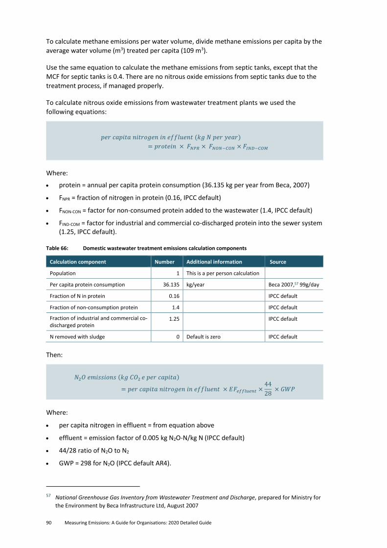
90 Measuring Emissions: A Guide for Organisations: 2020 Detailed Guide
To calculate methane emissions per water volume, divide methane emissions per capita by the
average water volume (m3) treated per capita (109 m3).
Use the same equation to calculate the methane emissions from septic tanks, except that the
MCF for septic tanks is 0.4. There are no nitrous oxide emissions from septic tanks due to the
treatment process, if managed properly.
To calculate nitrous oxide emissions from wastewater treatment plants we used the
following equations:
𝑝𝑒𝑟 𝑐𝑎𝑝𝑖𝑡𝑎 𝑛𝑖𝑡𝑟𝑜𝑔𝑒𝑛 𝑖𝑛 𝑒𝑓𝑓𝑙𝑢𝑒𝑛𝑡 (𝑘𝑔 𝑁 𝑝𝑒𝑟 𝑦𝑒𝑎𝑟)
= 𝑝𝑟𝑜𝑡𝑒𝑖𝑛 × 𝐹𝑁𝑃𝑅 × 𝐹𝑁𝑂𝑁−𝐶𝑂𝑁 × 𝐹𝐼𝑁𝐷−𝐶𝑂𝑀
Where:
• protein = annual per capita protein consumption (36.135 kg per year from Beca, 2007)
• FNPR = fraction of nitrogen in protein (0.16, IPCC default)
• FNON-CON = factor for non-consumed protein added to the wastewater (1.4, IPCC default)
• FIND-COM = factor for industrial and commercial co-discharged protein into the sewer system (1.25, IPCC default).
Table 66: Domestic wastewater treatment emissions calculation components
Calculation component Number Additional information Source
Population 1 This is a per person calculation
Per capita protein consumption 36.135 kg/year Beca 2007,57 99g/day
Fraction of N in protein 0.16 IPCC default
Fraction of non-consumption protein 1.4 IPCC default
Fraction of industrial and commercial co-discharged protein
1.25 IPCC default
N removed with sludge 0 Default is zero IPCC default
Then:
𝑁2𝑂 𝑒𝑚𝑖𝑠𝑠𝑖𝑜𝑛𝑠 (𝑘𝑔 𝐶𝑂2 𝑒 𝑝𝑒𝑟 𝑐𝑎𝑝𝑖𝑡𝑎)
= 𝑝𝑒𝑟 𝑐𝑎𝑝𝑖𝑡𝑎 𝑛𝑖𝑡𝑟𝑜𝑔𝑒𝑛 𝑖𝑛 𝑒𝑓𝑓𝑙𝑢𝑒𝑛𝑡 × 𝐸𝐹𝑒𝑓𝑓𝑙𝑢𝑒𝑛𝑡 ×44
28 × 𝐺𝑊𝑃
Where:
• per capita nitrogen in effluent = from equation above
• effluent = emission factor of 0.005 kg N2O-N/kg N (IPCC default)
• 44/28 ratio of N2O to N2
• GWP = 298 for N2O (IPCC default AR4).
57 National Greenhouse Gas Inventory from Wastewater Treatment and Discharge, prepared for Ministry for
the Environment by Beca Infrastructure Ltd, August 2007

Measuring Emissions: A Guide for Organisations: 2020 Detailed Guide 91
Divide these emissions per capita by the average volume of water treated (109 m3) per person
to give the emissions per m3.
Industrial wastewater treatment
As with domestic wastewater, we derived the emission factors for industrial wastewater
treatment from the total energy-use emissions in the wastewater treatment plants and the
gases emitted during the treatment process.
For the purpose of this guide, it is assumed there are no direct carbon dioxide emissions from
the treatment of wastewater, as all carbon dioxide emissions are biogenic. Therefore we have
calculated only methane and nitrous oxide emissions.
The equation followed to calculate methane emissions is:
𝑚𝑏𝐶𝑂𝐷 × 𝐸𝐹 × 𝐺𝑊𝑃 = 𝑚𝑒𝑡ℎ𝑎𝑛𝑒 𝑒𝑚𝑖𝑠𝑠𝑖𝑜𝑛 𝑓𝑎𝑐𝑡𝑜𝑟 (𝑘𝑔/𝑢𝑛𝑖𝑡)
Where:
• mbCOD = the unit biodegradable chemical oxygen demand load in kg per tonne of material processed (specified by industry type in table 55: Calculating the ratio of gases in diesel) (kg CODb)/t
• EF = emission factor in kg methane/kg COD
• GWP = global warming potential.
The following tables (table 67 and table 68) detail the information used in the calculations to
provide the industrial wastewater treatment emission factors.
Table 67: Industrial wastewater treatment methane emissions calculation information
Factor
Industry
Source
Pulp and
paper
Meat (excluding
poultry) Poultry Wine
Biodegradable chemical
oxygen demand load
(kg CODb/tonne)
36 50 50 12.42 Cardno (2015)
CH4 emission factor
(kg CH4/kg CODb)
0.0117 0.03575 0.034375 0.016661 Cardno (2015)
GWP 25 25 25 25 IPCC default AR4
It is assumed that the methods used to treat wastewater from dairy processing do not result in
methane emissions.
The equation used to calculate nitrous oxide emissions is:
𝑚𝑏𝐶𝑂𝐷 × 𝑁: 𝐶𝑂𝐷 × 𝐸𝐹 × (44
28) × 𝐺𝑊𝑃 = 𝑁 = 𝑛𝑖𝑡𝑟𝑜𝑢𝑠 𝑜𝑥𝑖𝑑𝑒 𝑒𝑚𝑖𝑠𝑠𝑖𝑜𝑛 𝑓𝑎𝑐𝑡𝑜𝑟 (
𝑘𝑔
𝑡𝑜𝑛𝑛𝑒𝑠)
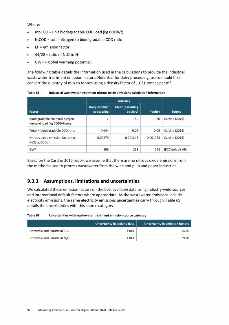
92 Measuring Emissions: A Guide for Organisations: 2020 Detailed Guide
Where:
• mbCOD = unit biodegradable COD load (kg CODb/t)
• N:COD = total nitrogen to biodegradable COD ratio
• EF = emission factor
• 44/28 = ratio of N2O to N2
• GWP = global warming potential.
The following table details the information used in the calculations to provide the industrial
wastewater treatment emission factors. Note that for dairy processing, users should first
convert the quantity of milk to tonnes using a density factor of 1.031 tonnes per m3.
Table 68: Industrial wastewater treatment nitrous oxide emissions calculation information
Factor
Industry
Source
Dairy product
processing
Meat (excluding
poultry) Poultry
Biodegradable chemical oxygen
demand load (kg CODb/tonne)
2 50 50 Cardno (2015)
Total N:biodegradable COD ratio 0.044 0.09 0.09 Cardno (2015)
Nitrous oxide emission factor (kg
N2O/kg CODb)
0.00279 0.001348 0.001925 Cardno (2015)
GWP 298 298 298 IPCC default AR4
Based on the Cardno 2015 report we assume that there are no nitrous oxide emissions from
the methods used to process wastewater from the wine and pulp and paper industries.
9.3.3 Assumptions, limitations and uncertainties
We calculated these emission factors on the best available data using industry-wide sources
and international default factors where appropriate. As the wastewater emissions include
electricity emissions, the same electricity emissions uncertainties carry through. Table 69
details the uncertainties with this source category.
Table 69: Uncertainties with wastewater treatment emission source category
Uncertainty in activity data Uncertainty in emission factors
Domestic and industrial CH4 ±10% ±40%
Domestic and industrial N2O ±10% ±90%
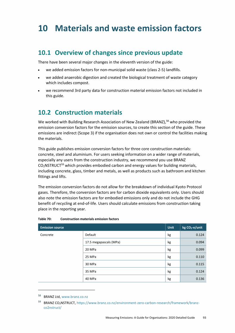
Measuring Emissions: A Guide for Organisations: 2020 Detailed Guide 93
10 Materials and waste emission factors
10.1 Overview of changes since previous update There have been several major changes in the eleventh version of the guide:
• we added emission factors for non-municipal solid waste (class 2-5) landfills.
• we added anaerobic digestion and created the biological treatment of waste category which includes compost.
• we recommend 3rd party data for construction material emission factors not included in this guide.
10.2 Construction materials We worked with Building Research Association of New Zealand (BRANZ),58 who provided the
emission conversion factors for the emission sources, to create this section of the guide. These
emissions are indirect (Scope 3) if the organisation does not own or control the facilities making
the materials.
This guide publishes emission conversion factors for three core construction materials:
concrete, steel and aluminium. For users seeking information on a wider range of materials,
especially any users from the construction industry, we recommend you use BRANZ
CO2NSTRUCT59 which provides embodied carbon and energy values for building materials,
including concrete, glass, timber and metals, as well as products such as bathroom and kitchen
fittings and lifts.
The emission conversion factors do not allow for the breakdown of individual Kyoto Protocol
gases. Therefore, the conversion factors are for carbon dioxide equivalents only. Users should
also note the emission factors are for embodied emissions only and do not include the GHG
benefit of recycling at end-of-life. Users should calculate emissions from construction taking
place in the reporting year.
Table 70: Construction materials emission factors
Emission source Unit kg CO2-e/unit
Concrete Default kg 0.124
17.5 megapascals (MPa) kg 0.094
20 MPa kg 0.099
25 MPa kg 0.110
30 MPa kg 0.115
35 MPa kg 0.124
40 MPa kg 0.136
58 BRANZ Ltd, www.branz.co.nz 59 BRANZ CO2NSTRUCT, https://www.branz.co.nz/environment-zero-carbon-research/framework/branz-
co2nstruct/
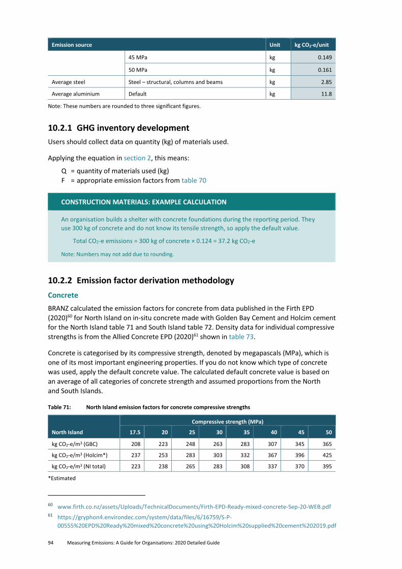
94 Measuring Emissions: A Guide for Organisations: 2020 Detailed Guide
Emission source Unit kg CO2-e/unit
45 MPa kg 0.149
50 MPa kg 0.161
Average steel Steel – structural, columns and beams kg 2.85
Average aluminium Default kg 11.8
Note: These numbers are rounded to three significant figures.
10.2.1 GHG inventory development
Users should collect data on quantity (kg) of materials used.
Applying the equation in section 2, this means:
Q = quantity of materials used (kg)
F = appropriate emission factors from table 70
CONSTRUCTION MATERIALS: EXAMPLE CALCULATION
An organisation builds a shelter with concrete foundations during the reporting period. They
use 300 kg of concrete and do not know its tensile strength, so apply the default value.
Total CO2-e emissions = 300 kg of concrete × 0.124 = 37.2 kg CO2-e
Note: Numbers may not add due to rounding.
10.2.2 Emission factor derivation methodology
Concrete
BRANZ calculated the emission factors for concrete from data published in the Firth EPD
(2020)60 for North Island on in-situ concrete made with Golden Bay Cement and Holcim cement
for the North Island table 71 and South Island table 72. Density data for individual compressive
strengths is from the Allied Concrete EPD (2020)61 shown in table 73.
Concrete is categorised by its compressive strength, denoted by megapascals (MPa), which is
one of its most important engineering properties. If you do not know which type of concrete
was used, apply the default concrete value. The calculated default concrete value is based on
an average of all categories of concrete strength and assumed proportions from the North
and South Islands.
Table 71: North Island emission factors for concrete compressive strengths
North Island
Compressive strength (MPa)
17.5 20 25 30 35 40 45 50
kg CO2-e/m3 (GBC) 208 223 248 263 283 307 345 365
kg CO2-e/m3 (Holcim*) 237 253 283 303 332 367 396 425
kg CO2-e/m3 (NI total) 223 238 265 283 308 337 370 395
*Estimated
60 www.firth.co.nz/assets/Uploads/TechnicalDocuments/Firth-EPD-Ready-mixed-concrete-Sep-20-WEB.pdf 61 https://gryphon4.environdec.com/system/data/files/6/16759/S-P-
00555%20EPD%20Ready%20mixed%20concrete%20using%20Holcim%20supplied%20cement%202019.pdf
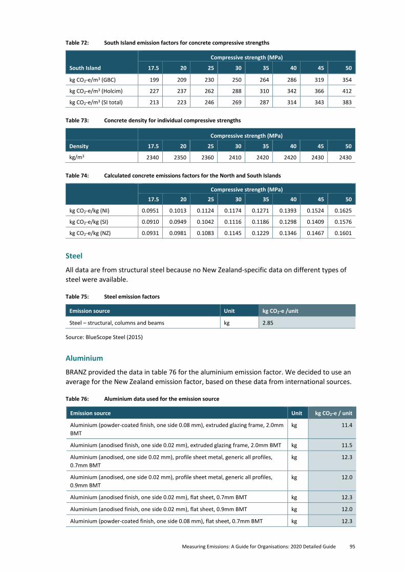
Measuring Emissions: A Guide for Organisations: 2020 Detailed Guide 95
Table 72: South Island emission factors for concrete compressive strengths
South Island
Compressive strength (MPa)
17.5 20 25 30 35 40 45 50
kg CO2-e/m3 (GBC) 199 209 230 250 264 286 319 354
kg CO2-e/m3 (Holcim) 227 237 262 288 310 342 366 412
kg CO2-e/m3 (SI total) 213 223 246 269 287 314 343 383
Table 73: Concrete density for individual compressive strengths
Compressive strength (MPa)
Density 17.5 20 25 30 35 40 45 50
kg/m3 2340 2350 2360 2410 2420 2420 2430 2430
Table 74: Calculated concrete emissions factors for the North and South Islands
Compressive strength (MPa)
17.5 20 25 30 35 40 45 50
kg CO2-e/kg (NI) 0.0951 0.1013 0.1124 0.1174 0.1271 0.1393 0.1524 0.1625
kg CO2-e/kg (SI) 0.0910 0.0949 0.1042 0.1116 0.1186 0.1298 0.1409 0.1576
kg CO2-e/kg (NZ) 0.0931 0.0981 0.1083 0.1145 0.1229 0.1346 0.1467 0.1601
Steel
All data are from structural steel because no New Zealand-specific data on different types of
steel were available.
Table 75: Steel emission factors
Emission source Unit kg CO2-e /unit
Steel – structural, columns and beams kg 2.85
Source: BlueScope Steel (2015)
Aluminium
BRANZ provided the data in table 76 for the aluminium emission factor. We decided to use an
average for the New Zealand emission factor, based on these data from international sources.
Table 76: Aluminium data used for the emission source
Emission source Unit kg CO2-e / unit
Aluminium (powder-coated finish, one side 0.08 mm), extruded glazing frame, 2.0mm
BMT
kg 11.4
Aluminium (anodised finish, one side 0.02 mm), extruded glazing frame, 2.0mm BMT kg 11.5
Aluminium (anodised, one side 0.02 mm), profile sheet metal, generic all profiles,
0.7mm BMT
kg 12.3
Aluminium (anodised, one side 0.02 mm), profile sheet metal, generic all profiles,
0.9mm BMT
kg 12.0
Aluminium (anodised finish, one side 0.02 mm), flat sheet, 0.7mm BMT kg 12.3
Aluminium (anodised finish, one side 0.02 mm), flat sheet, 0.9mm BMT kg 12.0
Aluminium (powder-coated finish, one side 0.08 mm), flat sheet, 0.7mm BMT kg 12.3
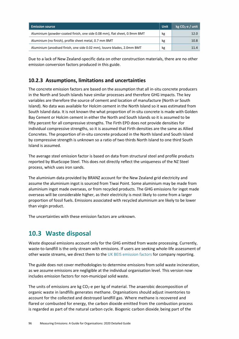
96 Measuring Emissions: A Guide for Organisations: 2020 Detailed Guide
Emission source Unit kg CO2-e / unit
Aluminium (powder-coated finish, one side 0.08 mm), flat sheet, 0.9mm BMT kg 12.0
Aluminium (no finish), profile sheet metal, 0.7 mm BMT kg 10.8
Aluminium (anodised finish, one side 0.02 mm), louvre blades, 2.0mm BMT kg 11.4
Due to a lack of New Zealand-specific data on other construction materials, there are no other
emission conversion factors produced in this guide.
10.2.3 Assumptions, limitations and uncertainties
The concrete emission factors are based on the assumption that all in-situ concrete producers
in the North and South Islands have similar processes and therefore GHG impacts. The key
variables are therefore the source of cement and location of manufacture (North or South
Island). No data was available for Holcim cement in the North Island so it was estimated from
South Island data. It is not known the what proportion of in-situ concrete is made with Golden
Bay Cement or Holcim cement in either the North and South Islands so it is assumed to be
fifty percent for all compressive strengths. The Firth EPD does not provide densities for
individual compressive strengths, so it is assumed that Firth densities are the same as Allied
Concretes. The proportion of in-situ concrete produced in the North Island and South Island
by compressive strength is unknown so a ratio of two thirds North Island to one third South
Island is assumed.
The average steel emission factor is based on data from structural steel and profile products
reported by BlueScope Steel. This does not directly reflect the uniqueness of the NZ Steel
process, which uses iron sands.
The aluminium data provided by BRANZ account for the New Zealand grid electricity and
assume the aluminium ingot is sourced from Tiwai Point. Some aluminium may be made from
aluminium ingot made overseas, or from recycled products. The GHG emissions for ingot made
overseas will be considerable higher, as their electricity is most likely to come from a larger
proportion of fossil fuels. Emissions associated with recycled aluminium are likely to be lower
than virgin product.
The uncertainties with these emission factors are unknown.
10.3 Waste disposal Waste disposal emissions account only for the GHG emitted from waste processing. Currently,
waste-to-landfill is the only stream with emissions. If users are seeking whole-life assessment of
other waste streams, we direct them to the UK BEIS emission factors for company reporting.
The guide does not cover methodologies to determine emissions from solid waste incineration,
as we assume emissions are negligible at the individual organisation level. This version now
includes emission factors for non-municipal solid waste.
The units of emissions are kg CO2-e per kg of material. The anaerobic decomposition of
organic waste in landfills generates methane. Organisations should adjust inventories to
account for the collected and destroyed landfill gas. Where methane is recovered and
flared or combusted for energy, the carbon dioxide emitted from the combustion process
is regarded as part of the natural carbon cycle. Biogenic carbon dioxide, being part of the
Measuring Emissions: A Guide for Organisations: 2020 Detailed Guide 97
natural cycle, is absorbed by living organic matter and released at the end of its life, and is
not included in these emission factors.
This update includes an emission factor for anaerobic digestion and this is grouped with
composting as a form of biological treatment of waste.
The type of landfill influences the GHG conversion factor, based on whether there is a methane
gas collection system.
Table 77: Description of landfill types
Landfill type Description
Municipal (class 1) landfills
With gas recovery
Municipal, well-managed Landfill where some of the CH4 produced during the
organic decomposition of waste is captured.
Municipal (class 1) landfills
Without gas recovery
Municipal, well-managed Landfill where the CH4 produced during organic
decomposition of waste escapes into the atmosphere.
Non-municipal (class 2-4)
landfills
Non-municipal landfills that accept a broader range of wastes where the CH4
produced during organic decomposition of waste escapes into the atmosphere.
Appendix C: Landfills with and without landfill gas recovery includes a list of class 1 landfills
with gas recovery.
If organisations are interested in calculating the emissions from recycling materials, they could
do so by independently accounting for the distance travelled by the waste to the recycling
plant, using freight emission factors (see section 8).
We calculated the waste-to-landfill emission conversion factors based on the national
inventory. table 78, table 79 and table 81 show the factors.
Table 78: Waste disposal to municipal (class 1) landfills with gas recovery
Emission source Unit kg CO2-e/unit
kg CO2/unit
(kg CO2-e)
kg CH4/unit
(kg CO2-e)
kg N2O/unit
(kg CO2-e)
Waste (known
composition)
Food kg 0.299 n/a 0.299 n/a
Garden kg 0.398 n/a 0.398 n/a
Paper kg 0.797 n/a 0.797 n/a
Wood kg 0.856 n/a 0.856 n/a
Textile kg 0.478 n/a 0.478 n/a
Nappies kg 0.478 n/a 0.478 n/a
Other (inert) kg n/a n/a n/a n/a
Waste (unknown
composition)
General waste kg 0.311 n/a 0.311 n/a
Office waste kg 0.489 n/a 0.489 n/a
Note: These numbers are rounded to three significant figures.
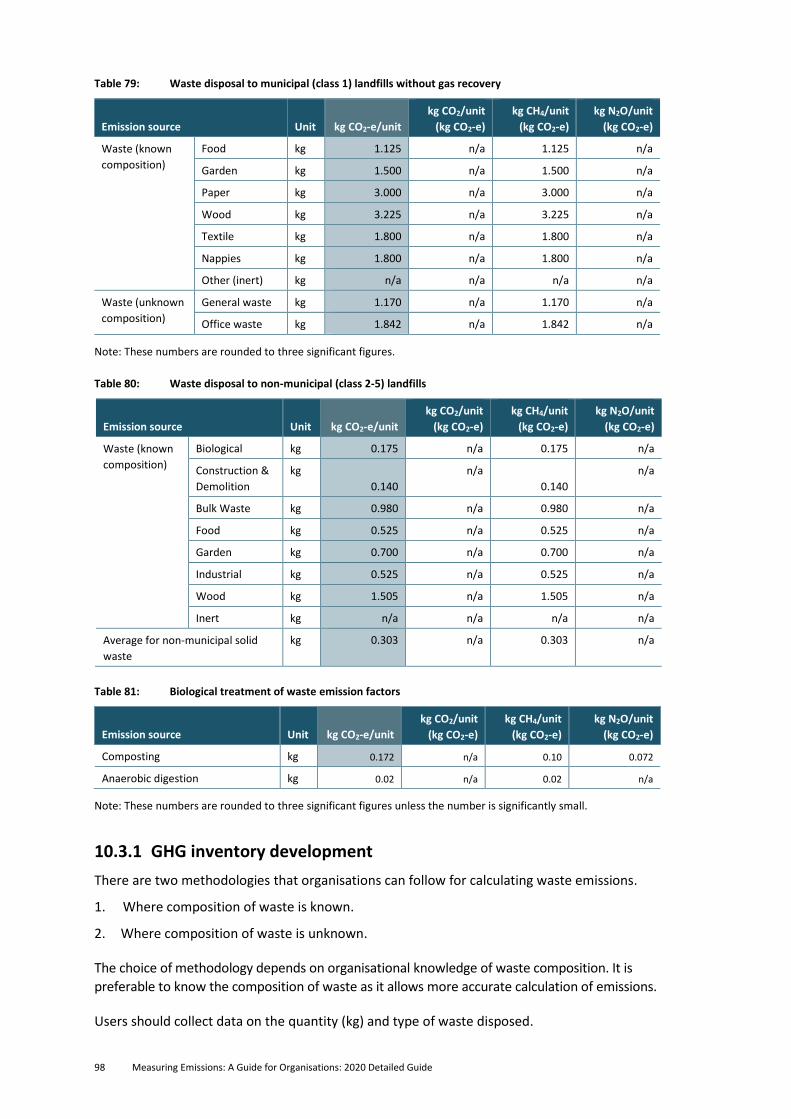
98 Measuring Emissions: A Guide for Organisations: 2020 Detailed Guide
Table 79: Waste disposal to municipal (class 1) landfills without gas recovery
Emission source Unit kg CO2-e/unit
kg CO2/unit
(kg CO2-e)
kg CH4/unit
(kg CO2-e)
kg N2O/unit
(kg CO2-e)
Waste (known
composition)
Food kg 1.125 n/a 1.125 n/a
Garden kg 1.500 n/a 1.500 n/a
Paper kg 3.000 n/a 3.000 n/a
Wood kg 3.225 n/a 3.225 n/a
Textile kg 1.800 n/a 1.800 n/a
Nappies kg 1.800 n/a 1.800 n/a
Other (inert) kg n/a n/a n/a n/a
Waste (unknown
composition)
General waste kg 1.170 n/a 1.170 n/a
Office waste kg 1.842 n/a 1.842 n/a
Note: These numbers are rounded to three significant figures.
Table 80: Waste disposal to non-municipal (class 2-5) landfills
Emission source Unit kg CO2-e/unit
kg CO2/unit
(kg CO2-e)
kg CH4/unit
(kg CO2-e)
kg N2O/unit
(kg CO2-e)
Waste (known
composition)
Biological kg 0.175 n/a 0.175 n/a
Construction &
Demolition
kg
0.140
n/a
0.140
n/a
Bulk Waste kg 0.980 n/a 0.980 n/a
Food kg 0.525 n/a 0.525 n/a
Garden kg 0.700 n/a 0.700 n/a
Industrial kg 0.525 n/a 0.525 n/a
Wood kg 1.505 n/a 1.505 n/a
Inert kg n/a n/a n/a n/a
Average for non-municipal solid
waste
kg 0.303 n/a 0.303 n/a
Table 81: Biological treatment of waste emission factors
Emission source Unit kg CO2-e/unit
kg CO2/unit
(kg CO2-e)
kg CH4/unit
(kg CO2-e)
kg N2O/unit
(kg CO2-e)
Composting kg 0.172 n/a 0.10 0.072
Anaerobic digestion kg 0.02 n/a 0.02 n/a
Note: These numbers are rounded to three significant figures unless the number is significantly small.
10.3.1 GHG inventory development
There are two methodologies that organisations can follow for calculating waste emissions.
1. Where composition of waste is known.
2. Where composition of waste is unknown.
The choice of methodology depends on organisational knowledge of waste composition. It is
preferable to know the composition of waste as it allows more accurate calculation of emissions.
Users should collect data on the quantity (kg) and type of waste disposed.
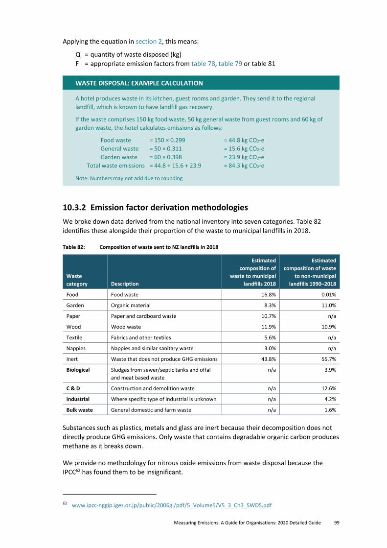
Measuring Emissions: A Guide for Organisations: 2020 Detailed Guide 99
Applying the equation in section 2, this means:
Q = quantity of waste disposed (kg)
F = appropriate emission factors from table 78, table 79 or table 81
WASTE DISPOSAL: EXAMPLE CALCULATION
A hotel produces waste in its kitchen, guest rooms and garden. They send it to the regional
landfill, which is known to have landfill gas recovery.
If the waste comprises 150 kg food waste, 50 kg general waste from guest rooms and 60 kg of
garden waste, the hotel calculates emissions as follows:
Food waste = 150 × 0.299 = 44.8 kg CO2-e
General waste = 50 × 0.311 = 15.6 kg CO2-e
Garden waste = 60 × 0.398 = 23.9 kg CO2-e
Total waste emissions = 44.8 + 15.6 + 23.9 = 84.3 kg CO2-e
Note: Numbers may not add due to rounding
10.3.2 Emission factor derivation methodologies
We broke down data derived from the national inventory into seven categories. Table 82
identifies these alongside their proportion of the waste to municipal landfills in 2018.
Table 82: Composition of waste sent to NZ landfills in 2018
Waste
category Description
Estimated
composition of
waste to municipal
landfills 2018
Estimated
composition of waste
to non-municipal
landfills 1990–2018
Food Food waste 16.8% 0.01%
Garden Organic material 8.3% 11.0%
Paper Paper and cardboard waste 10.7% n/a
Wood Wood waste 11.9% 10.9%
Textile Fabrics and other textiles 5.6% n/a
Nappies Nappies and similar sanitary waste 3.0% n/a
Inert Waste that does not produce GHG emissions 43.8% 55.7%
Biological Sludges from sewer/septic tanks and offal
and meat based waste
n/a 3.9%
C & D Construction and demolition waste n/a 12.6%
Industrial Where specific type of industrial is unknown n/a 4.2%
Bulk waste General domestic and farm waste n/a 1.6%
Substances such as plastics, metals and glass are inert because their decomposition does not
directly produce GHG emissions. Only waste that contains degradable organic carbon produces
methane as it breaks down.
We provide no methodology for nitrous oxide emissions from waste disposal because the
IPCC62 has found them to be insignificant.
62 www.ipcc-nggip.iges.or.jp/public/2006gl/pdf/5_Volume5/V5_3_Ch3_SWDS.pdf
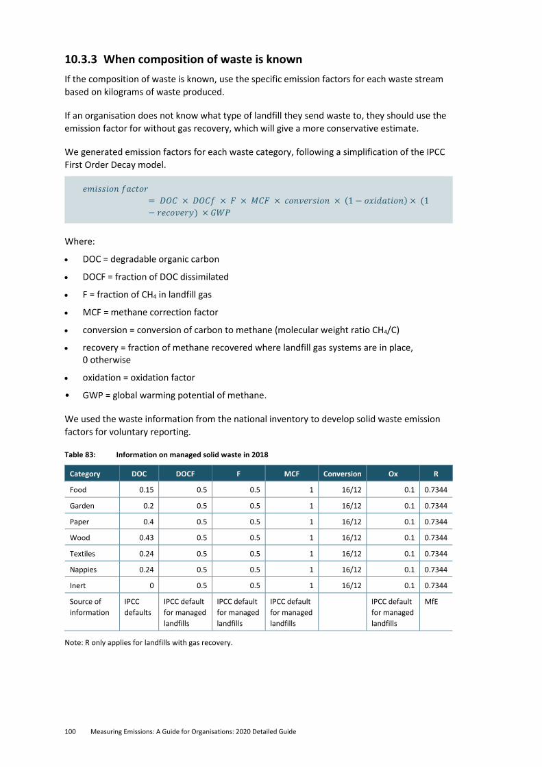
100 Measuring Emissions: A Guide for Organisations: 2020 Detailed Guide
10.3.3 When composition of waste is known
If the composition of waste is known, use the specific emission factors for each waste stream
based on kilograms of waste produced.
If an organisation does not know what type of landfill they send waste to, they should use the
emission factor for without gas recovery, which will give a more conservative estimate.
We generated emission factors for each waste category, following a simplification of the IPCC
First Order Decay model.
𝑒𝑚𝑖𝑠𝑠𝑖𝑜𝑛 𝑓𝑎𝑐𝑡𝑜𝑟
= 𝐷𝑂𝐶 × 𝐷𝑂𝐶𝑓 × 𝐹 × 𝑀𝐶𝐹 × 𝑐𝑜𝑛𝑣𝑒𝑟𝑠𝑖𝑜𝑛 × (1 − 𝑜𝑥𝑖𝑑𝑎𝑡𝑖𝑜𝑛) × (1
− 𝑟𝑒𝑐𝑜𝑣𝑒𝑟𝑦) × 𝐺𝑊𝑃
Where:
• DOC = degradable organic carbon
• DOCF = fraction of DOC dissimilated
• F = fraction of CH4 in landfill gas
• MCF = methane correction factor
• conversion = conversion of carbon to methane (molecular weight ratio CH4/C)
• recovery = fraction of methane recovered where landfill gas systems are in place, 0 otherwise
• oxidation = oxidation factor
• GWP = global warming potential of methane.
We used the waste information from the national inventory to develop solid waste emission
factors for voluntary reporting.
Table 83: Information on managed solid waste in 2018
Category DOC DOCF F MCF Conversion Ox R
Food 0.15 0.5 0.5 1 16/12 0.1 0.7344
Garden 0.2 0.5 0.5 1 16/12 0.1 0.7344
Paper 0.4 0.5 0.5 1 16/12 0.1 0.7344
Wood 0.43 0.5 0.5 1 16/12 0.1 0.7344
Textiles 0.24 0.5 0.5 1 16/12 0.1 0.7344
Nappies 0.24 0.5 0.5 1 16/12 0.1 0.7344
Inert 0 0.5 0.5 1 16/12 0.1 0.7344
Source of
information
IPCC
defaults
IPCC default
for managed
landfills
IPCC default
for managed
landfills
IPCC default
for managed
landfills
IPCC default
for managed
landfills
MfE
Note: R only applies for landfills with gas recovery.
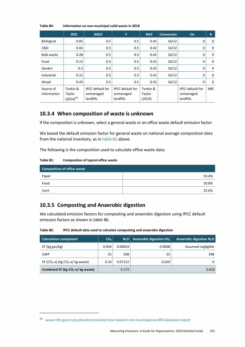
Measuring Emissions: A Guide for Organisations: 2020 Detailed Guide 101
Table 84: Information on non-municipal solid waste in 2018
DOC DOCF F MCF Conversion Ox R
Biological 0.05 0.5 0.5 0.42 16/12 0 0
C&D 0.04 0.5 0.5 0.42 16/12 0 0
Bulk waste 0.28 0.5 0.5 0.42 16/12 0 0
Food 0.15 0.5 0.5 0.42 16/12 0 0
Garden 0.2 0.5 0.5 0.42 16/12 0 0
Industrial 0.15 0.5 0.5 0.42 16/12 0 0
Wood 0.43 0.5 0.5 0.42 16/12 0 0
Source of
information
Tonkin &
Taylor
(2014)63
IPCC default for
unmanaged
landfills
IPCC default for
unmanaged
landfills
Tonkin &
Taylor
(2014)
IPCC default for
unmanaged
landfills
MfE
10.3.4 When composition of waste is unknown
If the composition is unknown, select a general waste or an office waste default emission factor.
We based the default emission factor for general waste on national average composition data
from the national inventory, as in table 82 above.
The following is the composition used to calculate office waste data.
Table 85: Composition of typical office waste
Composition of office waste
Paper 53.6%
Food 20.8%
Inert 25.6%
10.3.5 Composting and Anaerobic digestion
We calculated emission factors for composting and anaerobic digestion using IPCC default
emission factors as shown in table 86.
Table 86: IPCC default data used to calculate composting and anaerobic digestion
Calculation component CH4 N2O Anaerobic digestion CH4 Anaerobic digestion N2O
EF (kg gas/kg) 0.004 0.00024 0.0008 Assumed negligible
GWP 25 298 25 298
EF (CO2-e) (kg CO2-e/ kg waste) 0.10 0.07152 0.020 0
Combined EF (kg CO2-e/ kg waste) 0.172 0.020
63 www.mfe.govt.nz/publications/waste/new-zealand-non-municipal-landfill-database-report
102 Measuring Emissions: A Guide for Organisations: 2020 Detailed Guide
10.3.6 Assumptions, limitations and uncertainties
The uncertainties for emission factors used in methane emissions from managed municipal
landfills is ±40 per cent. This is consistent with the estimates in the IPCC Guidelines (IPCC,
2006a). The national inventory states that “It is set at this level because some, but not all, of
the estimates for methane recovery are based on metered gas-flow data”.
If an organisation has an advanced diversion system (to recycling and composting) then using
the ‘mixed waste’ category in the methodology will overestimate emissions. If an organisation
has no diversion system, then it could underestimate emissions.
The default emission factor for mixed waste is based on national average composition
data from the national inventory. Only waste to municipal and non-municipal landfills
are considered.
Previously, the emission factors for office waste represented an assumed default composition
(paper 53.6 per cent, garden and food 20.8 per cent and wood 0 per cent) for office waste,
based on waste data from government buildings. We separated garden and food waste in this
version of the guide, and assume that food represents all waste previously allocated to that
category. We assume the remaining 25.6 per cent is inert material.
Measuring Emissions: A Guide for Organisations: 2020 Detailed Guide 103
11 Agriculture, forestry and other land use emission factors
This category covers emissions produced by land use, land-use change and forestry
(LULUCF), livestock enteric fermentation, manure management and fertiliser use. Including
these sources is in line with New Zealand’s Greenhouse Gas Inventory 1990–2018.
We selected the emission factors below, based on appropriate available data and the
professional opinions of the Ministry for Primary Industries (MPI) and the Ministry for
the Environment.
• Land use, land-use change and forestry
− forest growth
− forest harvest and deforestation
• Agriculture
− enteric fermentation
− manure management
− fertiliser use
− agricultural soils (livestock).
Users should disclose in their inventories if they include animals grazing on land not owned by
the organisation.
11.1 Overview of changes since previous update This version of the guide includes additional emission factors for animal species including
swine, goats, horses, alpaca, mules, asses and poultry. This guide uses data from the
New Zealand Greenhouse Inventory which has revised methodologies and emissions
factors from the previous edition. These are summarised as:
• use of new N2O emission factors from animal excreta split by stock type and hill slope, applied using a new model to calculate the amount of livestock excreta deposited onto the different slopes: low (gradient between 0 degrees and 12 degrees), medium (between 12 degrees and 24 degrees) and steep (greater than 24 degrees gradient)
• use of revised activity data for the proportion of dairy goats in the overall farmed goat population
• minor improvements to the equations used to estimate energy efficiency for maintenance for beef cattle, sheep and deer, including the specification of a constant to more significant figures and reverting to the IPCC default value of 18.45 megajoules per kilogram of dry matter (MJ/kg DM) for the gross energy content of feed (from the previous values of 18.40 MJ/kg DM for cattle and deer, and 18.50 MJ/kg DM for sheep).
Please refer to section 5.1.5 (and other relevant sections) New Zealand’s Greenhouse Inventory
1990–2018 for further details.64
64 www.mfe.govt.nz/sites/default/files/media/Climate%20Change/new-zealands-greenhouse-gas-inventory-
1990-2018-vol-1.pdf
104 Measuring Emissions: A Guide for Organisations: 2020 Detailed Guide
11.2 Land use, land-use change and forestry (LULUCF)
11.2.1 Overview of the sector
GHG emissions from vegetation and soils due to human activities are reported in the land use,
land-use change and forestry (LULUCF) sector. This guide provides emission factors related to
forest growth, forest harvest and deforestation only. The term LULUCF is used for consistency
with the national inventory.
The LULUCF sector is responsible for both emitting GHG to the atmosphere (emissions ie,
through harvesting and deforestation) and removing GHG from the atmosphere (removals
ie, through vegetation growth and increasing organic carbon stored in soils). Most emissions
reported in this sector are due to forestry activities such as harvest operations in production
forests, and most removals are due to forest growth.
The basis for the methods given here is that the flux of carbon dioxide to and from the
atmosphere is due to the changes in carbon stocks in vegetation and soils. When emissions
exceed removals, LULUCF is a ‘net source’ and emissions are positive. When removals exceed
emissions, LULUCF is a ‘net sink’ and emissions are negative.
The guide provides methods to estimate the carbon stock change (or flux) that occurs from
forestry activities during the applicable measurement period. We do not provide methods
here to estimate carbon stock changes in non-forest vegetation, soils, harvested wood
products, or for the associated nitrous oxide and methane emissions. For more detail, see
the national inventory.
In line with ISO 14064-1:2018 and the GHG Protocol, organisations should consider LULUCF
emissions if they have forest land within their measurement boundary, or own land that has
been deforested during the measurement period.
Organisations with LULUCF emissions should calculate and report these separately from direct
and indirect (Scope 1, 2 and 3) emissions.
The emission factors in this guide are New Zealand-specific, derived from national averages.
Although the main aim of this section of the guide is to estimate stock changes from forestry
activities, it can also be used to estimate the total carbon stored for a given forest type in a
given area. This can help organisations understand the potential impact of some forestry
activities on emissions, and how to manage land use for carbon.
11.2.2 LULUCF emission factors
Planted forests
The emission factor for planted forest growth (shown in table 87) is based on the Land Use and
Carbon Analysis System (LUCAS) national sample. It represents the average annual increment
over 28 years. Note the emission factor accounts for both the gains from forest growth and
losses from any forest management activities up until the point of harvest.
The emission factor for planted forest harvest and deforestation is in table 88.
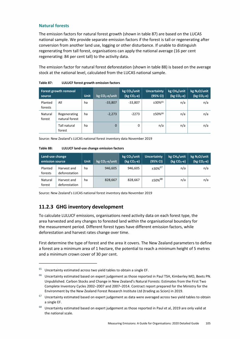
Measuring Emissions: A Guide for Organisations: 2020 Detailed Guide 105
Natural forests
The emission factors for natural forest growth (shown in table 87) are based on the LUCAS
national sample. We provide separate emission factors if the forest is tall or regenerating after
conversion from another land use, logging or other disturbance. If unable to distinguish
regenerating from tall forest, organisations can apply the national average (16 per cent
regenerating: 84 per cent tall) to the activity data.
The emission factor for natural forest deforestation (shown in table 88) is based on the average
stock at the national level, calculated from the LUCAS national sample.
Table 87: LULUCF forest growth emission factors
Forest growth removal
source Unit kg CO2-e/unit
kg CO2/unit
(kg CO2-e)
Uncertainty
(95% CI)
kg CH4/unit
(kg CO2-e)
kg N2O/unit
(kg CO2-e)
Planted
forests
All ha -33,807 -33,807 ±30%65 n/a n/a
Natural
forest
Regenerating
natural forest
ha -2,273 -2273 ±50%66 n/a n/a
Tall natural
forest
ha 0 0 n/a n/a n/a
Source: New Zealand’s LUCAS national forest inventory data November 2019
Table 88: LULUCF land-use change emission factors
Land-use change
emission source Unit kg CO2-e/unit
kg CO2/unit
(kg CO2-e)
Uncertainty
(95% CI)
kg CH4/unit
(kg CO2-e)
kg N2O/unit
(kg CO2-e)
Planted
forests
Harvest and
deforestation
ha 946,605 946,605 ±30%67 n/a n/a
Natural
forest
Harvest and
deforestation
ha 828,667 828,667 ±50%68 n/a n/a
Source: New Zealand’s LUCAS national forest inventory data November 2019
11.2.3 GHG inventory development
To calculate LULUCF emissions, organisations need activity data on each forest type, the
area harvested and any changes to forested land within the organisational boundary for
the measurement period. Different forest types have different emission factors, while
deforestation and harvest rates change over time.
First determine the type of forest and the area it covers. The New Zealand parameters to define
a forest are a minimum area of 1 hectare, the potential to reach a minimum height of 5 metres
and a minimum crown cover of 30 per cent.
65 Uncertainty estimated across two yield tables to obtain a single EF. 66 Uncertainty estimated based on expert judgement as those reported in Paul TSH, Kimberley MO, Beets PN.
Unpublished. Carbon Stocks and Change in New Zealand’s Natural Forests: Estimates from the First Two
Complete Inventory Cycles 2002–2007 and 2007–2014. Contract report prepared for the Ministry for the
Environment by the New Zealand Forest Research Institute Ltd (trading as Scion) in 2019. 67 Uncertainty estimated based on expert judgement as data were averaged across two yield tables to obtain
a single EF. 68 Uncertainty estimated based on expert judgement as those reported in Paul et al, 2019 are only valid at
the national scale.
106 Measuring Emissions: A Guide for Organisations: 2020 Detailed Guide
Forest types:
1. Tall natural forest: comprises mature indigenous forest, and may contain self-sown exotic
trees, such as wilding pines.
2. Regenerating natural forest: comprises indigenous and naturally occurring vegetation,
including broadleaved hardwood shrubland, mānuka–kānuka and other woody shrubland,
with potential to reach forest under its current management.
3. Planted forest: plantations of forest species mainly used for forestry, including:
− radiata pine (Pinus radiata)
− Douglas fir (Pseudotsuga menziesii)
− eucalypts (Eucalyptus spp)
− other planted species (with potential to reach ≥ 5 metre height at maturity in situ).
Organisations will also need records of forest harvest and deforestation activities (including
area in ha) to calculate the emissions from LULUCF. Sources of this information include:
1. Corporate or farm records for enterprises and organisations.
2. Geospatial analysis of the property or region.
3. The LUCAS Land Use Map69 can provide area by vegetation type at 1990, 2008, 2012 and
2016. It requires geospatial expertise to analyse and extract the data by region. This is free to
use and supports users in monitoring changes in their own land management practices.
4. The New Zealand Land Cover Database (LCDB)70 provides multi-temporal land cover. It
requires geospatial expertise to analyse and extract the data for sub-national analysis.
Using the sources detailed above to gather information on the land use, forest type and size,
organisations can apply the equation in section 2:
Q = area of land (ha)
F = appropriate emission factors (for land use) from table 87 and table 88
LAND USE, LAND-USE CHANGE AND FORESTRY: EXAMPLE CALCULATION
An organisation owns 4 ha of land: 3 ha are planted forest and 1 ha is regenerating natural
forest. During the reporting year the organisation harvested the planted forest for timber.
3 ha of planted forest were harvested, therefore:
CO2 emissions = 3 × 946,605 = 2,839,815 kg CO2-e
The removals (expressed as a negative) for the regenerating natural forest are:
CO2 removals = 1 × -2,273 = -2,273 kg CO2e
Therefore, total net CO2-e emissions = 2,839,815 – 2,273 = 2,837,542 kg CO2-e.
Note: Negative emissions are a carbon sink.
69 Land Use Carbon Analysis System (LUCAS) Land Use Map available at https://data.mfe.govt.nz/
70 LCDB available at https://lris.scinfo.org.nz/layer/48423-lcdb-v41-land-cover-database-version-41-
mainland-new-zealand/
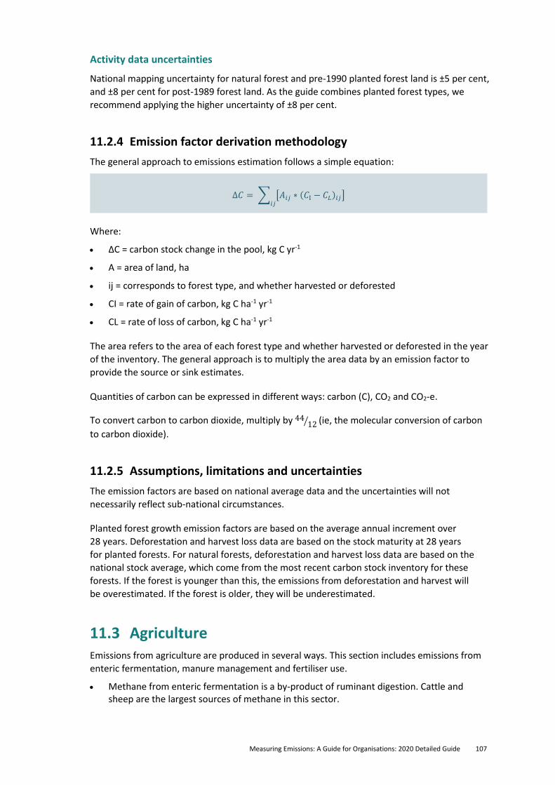
Measuring Emissions: A Guide for Organisations: 2020 Detailed Guide 107
Activity data uncertainties
National mapping uncertainty for natural forest and pre-1990 planted forest land is ±5 per cent,
and ±8 per cent for post-1989 forest land. As the guide combines planted forest types, we
recommend applying the higher uncertainty of ±8 per cent.
11.2.4 Emission factor derivation methodology
The general approach to emissions estimation follows a simple equation:
∆𝐶 = ∑ [𝐴𝑖𝑗 ∗ (𝐶I − 𝐶𝐿)𝑖𝑗]𝑖𝑗
Where:
• ∆C = carbon stock change in the pool, kg C yr-1
• A = area of land, ha
• ij = corresponds to forest type, and whether harvested or deforested
• CI = rate of gain of carbon, kg C ha-1 yr-1
• CL = rate of loss of carbon, kg C ha-1 yr-1
The area refers to the area of each forest type and whether harvested or deforested in the year
of the inventory. The general approach is to multiply the area data by an emission factor to
provide the source or sink estimates.
Quantities of carbon can be expressed in different ways: carbon (C), CO2 and CO2-e.
To convert carbon to carbon dioxide, multiply by 4412⁄ (ie, the molecular conversion of carbon
to carbon dioxide).
11.2.5 Assumptions, limitations and uncertainties
The emission factors are based on national average data and the uncertainties will not
necessarily reflect sub-national circumstances.
Planted forest growth emission factors are based on the average annual increment over
28 years. Deforestation and harvest loss data are based on the stock maturity at 28 years
for planted forests. For natural forests, deforestation and harvest loss data are based on the
national stock average, which come from the most recent carbon stock inventory for these
forests. If the forest is younger than this, the emissions from deforestation and harvest will
be overestimated. If the forest is older, they will be underestimated.
11.3 Agriculture Emissions from agriculture are produced in several ways. This section includes emissions from
enteric fermentation, manure management and fertiliser use.
• Methane from enteric fermentation is a by-product of ruminant digestion. Cattle and sheep are the largest sources of methane in this sector.
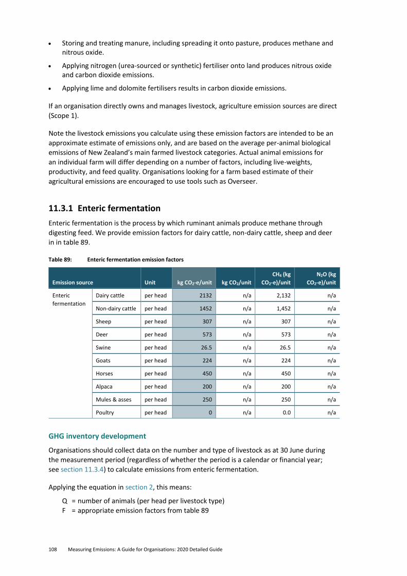
108 Measuring Emissions: A Guide for Organisations: 2020 Detailed Guide
• Storing and treating manure, including spreading it onto pasture, produces methane and nitrous oxide.
• Applying nitrogen (urea-sourced or synthetic) fertiliser onto land produces nitrous oxide and carbon dioxide emissions.
• Applying lime and dolomite fertilisers results in carbon dioxide emissions.
If an organisation directly owns and manages livestock, agriculture emission sources are direct
(Scope 1).
Note the livestock emissions you calculate using these emission factors are intended to be an
approximate estimate of emissions only, and are based on the average per-animal biological
emissions of New Zealand’s main farmed livestock categories. Actual animal emissions for
an individual farm will differ depending on a number of factors, including live-weights,
productivity, and feed quality. Organisations looking for a farm based estimate of their
agricultural emissions are encouraged to use tools such as Overseer.
11.3.1 Enteric fermentation
Enteric fermentation is the process by which ruminant animals produce methane through
digesting feed. We provide emission factors for dairy cattle, non-dairy cattle, sheep and deer
in in table 89.
Table 89: Enteric fermentation emission factors
Emission source Unit kg CO2-e/unit kg CO2/unit
CH4 (kg
CO2-e)/unit
N2O (kg
CO2-e)/unit
Enteric
fermentation
Dairy cattle per head 2132 n/a 2,132 n/a
Non-dairy cattle per head 1452 n/a 1,452 n/a
Sheep per head 307 n/a 307 n/a
Deer per head 573 n/a 573 n/a
Swine per head 26.5 n/a 26.5 n/a
Goats per head 224 n/a 224 n/a
Horses per head 450 n/a 450 n/a
Alpaca per head 200 n/a 200 n/a
Mules & asses per head 250 n/a 250 n/a
Poultry per head 0 n/a 0.0 n/a
GHG inventory development
Organisations should collect data on the number and type of livestock as at 30 June during
the measurement period (regardless of whether the period is a calendar or financial year;
see section 11.3.4) to calculate emissions from enteric fermentation.
Applying the equation in section 2, this means:
Q = number of animals (per head per livestock type)
F = appropriate emission factors from table 89

Measuring Emissions: A Guide for Organisations: 2020 Detailed Guide 109
ENTERIC FERMENTATION: EXAMPLE CALCULATION
An organisation owns 30 sheep and six dairy cows on 30 June during the reporting period.
They graze on land owned by the organisation.
CO2 emissions = 0
CH4 emissions = (30 × 307) + (6 × 2,132) = 22,002 kg CO2-e
N2O emissions = 0
Total CO2-e emissions = 22,002 kg CO2-e
Note: Numbers may not add due to rounding.
Emission factor derivation methodology
The national inventory publishes total emissions for enteric fermentation per livestock type,
along with population numbers. The Ministry of Primary Industries (MPI) supplied these same
data for the creation of emission factors. We used this information, shown in table 90, to
calculate the emission factors based on the following equation:
𝑒𝑚𝑖𝑠𝑠𝑖𝑜𝑛 𝑓𝑎𝑐𝑡𝑜𝑟 𝑝𝑒𝑟 𝑎𝑛𝑖𝑚𝑎𝑙 =𝑒𝑛𝑡𝑒𝑟𝑖𝑐 𝑓𝑒𝑟𝑚𝑒𝑛𝑡𝑎𝑡𝑖𝑜𝑛
𝑝𝑜𝑝𝑢𝑙𝑎𝑡𝑖𝑜𝑛
Note that the emission factors are based on data supplied for the national inventory. To ensure
consistency, organisations should report their population of livestock as at 30 June, regardless
of the measurement period.
MPI defines non-dairy cattle as beef breeds of cattle, including dairy-beef, as well as any beef
breeding stock.
Table 90: Enteric fermentation figures per livestock type
Animal 2018 population
Enteric fermentation emissions in 2018
(kt CH4) (as GHG)
Dairy cattle 6,385,541 544.46
Non-dairy cattle 3,721,262 216.09
Sheep 27,295,749 335.6
Deer 851,424 19.5
Swine 279,049 7.39
Goats 88,785 19.89
Horses 40,370 18.17
Alpaca 8,769 1.75
Mules & asses 141 0.035
Poultry 17,949,985 n/a
Note: kt is kilotonne.
Source: Based on figures from the Agricultural Inventory Model used in New Zealand’s Greenhouse Gas Inventory
1990–2018.
The emission conversion factors are in the Emission Factors Workbook.
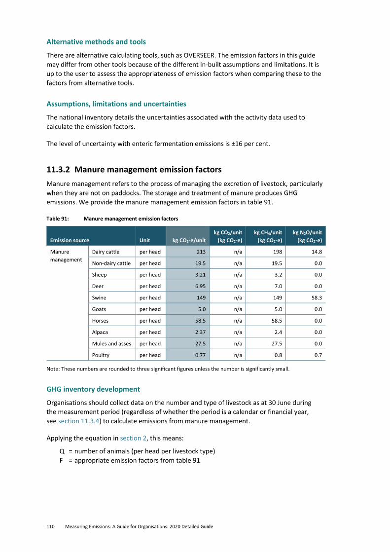
110 Measuring Emissions: A Guide for Organisations: 2020 Detailed Guide
Alternative methods and tools
There are alternative calculating tools, such as OVERSEER. The emission factors in this guide
may differ from other tools because of the different in-built assumptions and limitations. It is
up to the user to assess the appropriateness of emission factors when comparing these to the
factors from alternative tools.
Assumptions, limitations and uncertainties
The national inventory details the uncertainties associated with the activity data used to
calculate the emission factors.
The level of uncertainty with enteric fermentation emissions is ±16 per cent.
11.3.2 Manure management emission factors
Manure management refers to the process of managing the excretion of livestock, particularly
when they are not on paddocks. The storage and treatment of manure produces GHG
emissions. We provide the manure management emission factors in table 91.
Table 91: Manure management emission factors
Emission source Unit kg CO2-e/unit
kg CO2/unit
(kg CO2-e)
kg CH4/unit
(kg CO2-e)
kg N2O/unit
(kg CO2-e)
Manure
management
Dairy cattle per head 213 n/a 198 14.8
Non-dairy cattle per head 19.5 n/a 19.5 0.0
Sheep per head 3.21 n/a 3.2 0.0
Deer per head 6.95 n/a 7.0 0.0
Swine per head 149 n/a 149 58.3
Goats per head 5.0 n/a 5.0 0.0
Horses per head 58.5 n/a 58.5 0.0
Alpaca per head 2.37 n/a 2.4 0.0
Mules and asses per head 27.5 n/a 27.5 0.0
Poultry per head 0.77 n/a 0.8 0.7
Note: These numbers are rounded to three significant figures unless the number is significantly small.
GHG inventory development
Organisations should collect data on the number and type of livestock as at 30 June during
the measurement period (regardless of whether the period is a calendar or financial year,
see section 11.3.4) to calculate emissions from manure management.
Applying the equation in section 2, this means:
Q = number of animals (per head per livestock type)
F = appropriate emission factors from table 91
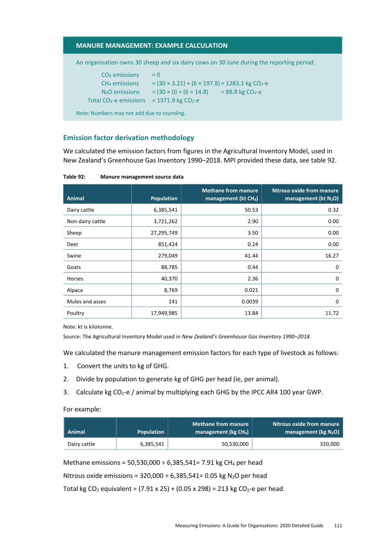
Measuring Emissions: A Guide for Organisations: 2020 Detailed Guide 111
MANURE MANAGEMENT: EXAMPLE CALCULATION
An organisation owns 30 sheep and six dairy cows on 30 June during the reporting period.
CO2 emissions = 0
CH4 emissions = (30 × 3.21) + (6 × 197.8) = 1283.1 kg CO2-e
N2O emissions = (30 × 0) + (6 × 14.8) = 88.8 kg CO2-e
Total CO2-e emissions = 1371.9 kg CO2-e
Note: Numbers may not add due to rounding.
Emission factor derivation methodology
We calculated the emission factors from figures in the Agricultural Inventory Model, used in
New Zealand’s Greenhouse Gas Inventory 1990–2018. MPI provided these data, see table 92.
Table 92: Manure management source data
Animal Population
Methane from manure
management (kt CH4)
Nitrous oxide from manure
management (kt N2O)
Dairy cattle 6,385,541 50.53 0.32
Non-dairy cattle 3,721,262 2.90 0.00
Sheep 27,295,749 3.50 0.00
Deer 851,424 0.24 0.00
Swine 279,049 41.44 16.27
Goats 88,785 0.44 0
Horses 40,370 2.36 0
Alpaca 8,769 0.021 0
Mules and asses 141 0.0039 0
Poultry 17,949,985 13.84 11.72
Note: kt is kilotonne.
Source: The Agricultural Inventory Model used in New Zealand’s Greenhouse Gas Inventory 1990–2018.
We calculated the manure management emission factors for each type of livestock as follows:
1. Convert the units to kg of GHG.
2. Divide by population to generate kg of GHG per head (ie, per animal).
3. Calculate kg CO2-e / animal by multiplying each GHG by the IPCC AR4 100 year GWP.
For example:
Animal Population
Methane from manure
management (kg CH4)
Nitrous oxide from manure
management (kg N2O)
Dairy cattle 6,385,541 50,530,000 320,000
Methane emissions = 50,530,000 ÷ 6,385,541= 7.91 kg CH4 per head
Nitrous oxide emissions = 320,000 ÷ 6,385,541= 0.05 kg N2O per head
Total kg CO2 equivalent = (7.91 x 25) + (0.05 x 298) = 213 kg CO2-e per head.
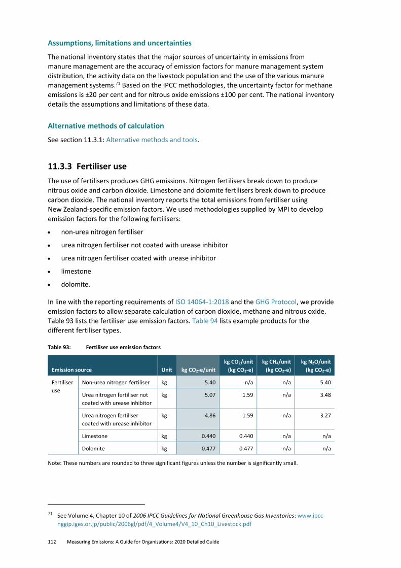
112 Measuring Emissions: A Guide for Organisations: 2020 Detailed Guide
Assumptions, limitations and uncertainties
The national inventory states that the major sources of uncertainty in emissions from
manure management are the accuracy of emission factors for manure management system
distribution, the activity data on the livestock population and the use of the various manure
management systems.71 Based on the IPCC methodologies, the uncertainty factor for methane
emissions is ±20 per cent and for nitrous oxide emissions ±100 per cent. The national inventory
details the assumptions and limitations of these data.
Alternative methods of calculation
See section 11.3.1: Alternative methods and tools.
11.3.3 Fertiliser use
The use of fertilisers produces GHG emissions. Nitrogen fertilisers break down to produce
nitrous oxide and carbon dioxide. Limestone and dolomite fertilisers break down to produce
carbon dioxide. The national inventory reports the total emissions from fertiliser using
New Zealand-specific emission factors. We used methodologies supplied by MPI to develop
emission factors for the following fertilisers:
• non-urea nitrogen fertiliser
• urea nitrogen fertiliser not coated with urease inhibitor
• urea nitrogen fertiliser coated with urease inhibitor
• limestone
• dolomite.
In line with the reporting requirements of ISO 14064-1:2018 and the GHG Protocol, we provide
emission factors to allow separate calculation of carbon dioxide, methane and nitrous oxide.
Table 93 lists the fertiliser use emission factors. Table 94 lists example products for the
different fertiliser types.
Table 93: Fertiliser use emission factors
Emission source Unit kg CO2-e/unit
kg CO2/unit
(kg CO2-e)
kg CH4/unit
(kg CO2-e)
kg N2O/unit
(kg CO2-e)
Fertiliser
use
Non-urea nitrogen fertiliser kg 5.40 n/a n/a 5.40
Urea nitrogen fertiliser not
coated with urease inhibitor
kg 5.07 1.59 n/a 3.48
Urea nitrogen fertiliser
coated with urease inhibitor
kg 4.86 1.59 n/a 3.27
Limestone kg 0.440 0.440 n/a n/a
Dolomite kg 0.477 0.477 n/a n/a
Note: These numbers are rounded to three significant figures unless the number is significantly small.
71 See Volume 4, Chapter 10 of 2006 IPCC Guidelines for National Greenhouse Gas Inventories: www.ipcc-
nggip.iges.or.jp/public/2006gl/pdf/4_Volume4/V4_10_Ch10_Livestock.pdf
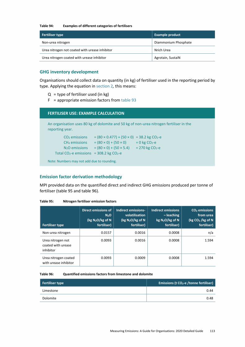
Measuring Emissions: A Guide for Organisations: 2020 Detailed Guide 113
Table 94: Examples of different categories of fertilisers
Fertiliser type Example product
Non-urea nitrogen Diammonium Phosphate
Urea nitrogen not coated with urease inhibitor Nrich Urea
Urea nitrogen coated with urease inhibitor Agrotain, SustaiN
GHG inventory development
Organisations should collect data on quantity (in kg) of fertiliser used in the reporting period by
type. Applying the equation in section 2, this means:
Q = type of fertiliser used (in kg)
F = appropriate emission factors from table 93
FERTILISER USE: EXAMPLE CALCULATION
An organisation uses 80 kg of dolomite and 50 kg of non-urea nitrogen fertiliser in the
reporting year.
CO2 emissions = (80 × 0.477) + (50 × 0) = 38.2 kg CO2-e
CH4 emissions = (80 × 0) + (50 × 0) = 0 kg CO2-e
N2O emissions = (80 × 0) + (50 × 5.4) = 270 kg CO2-e
Total CO2-e emissions = 308.2 kg CO2-e
Note: Numbers may not add due to rounding.
Emission factor derivation methodology
MPI provided data on the quantified direct and indirect GHG emissions produced per tonne of
fertiliser (table 95 and table 96).
Table 95: Nitrogen fertiliser emission factors
Fertiliser type
Direct emissions of
N2O
(kg N2O/kg of N
fertiliser)
Indirect emissions-
volatilisation
(kg N2O/kg of N
fertiliser)
Indirect emissions
– leaching
kg N2O/kg of N
fertiliser)
CO2 emissions
from urea
(kg CO2 /kg of N
fertiliser)
Non-urea nitrogen 0.0157 0.0016 0.0008 n/a
Urea nitrogen not
coated with urease
inhibitor
0.0093 0.0016 0.0008 1.594
Urea nitrogen coated
with urease inhibitor
0.0093 0.0009 0.0008 1.594
Table 96: Quantified emissions factors from limestone and dolomite
Fertiliser type Emissions (t CO2-e /tonne fertiliser)
Limestone 0.44
Dolomite 0.48
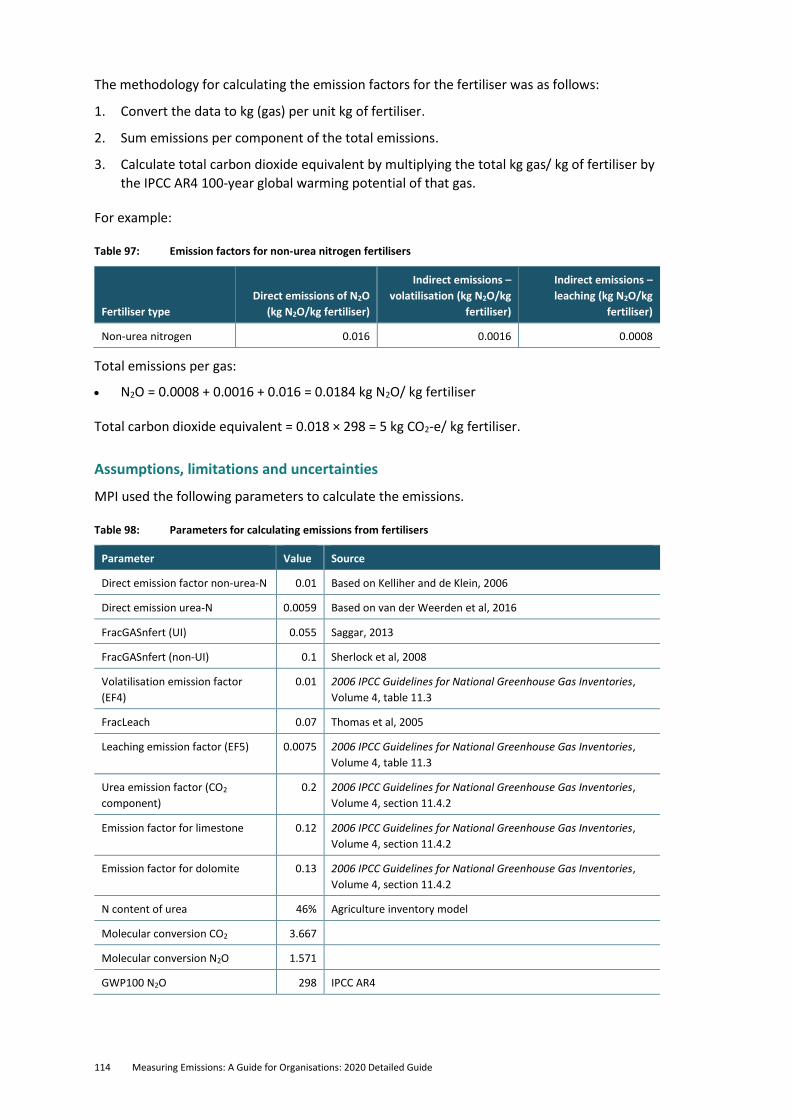
114 Measuring Emissions: A Guide for Organisations: 2020 Detailed Guide
The methodology for calculating the emission factors for the fertiliser was as follows:
1. Convert the data to kg (gas) per unit kg of fertiliser.
2. Sum emissions per component of the total emissions.
3. Calculate total carbon dioxide equivalent by multiplying the total kg gas/ kg of fertiliser by
the IPCC AR4 100-year global warming potential of that gas.
For example:
Table 97: Emission factors for non-urea nitrogen fertilisers
Fertiliser type
Direct emissions of N2O
(kg N2O/kg fertiliser)
Indirect emissions –
volatilisation (kg N2O/kg
fertiliser)
Indirect emissions –
leaching (kg N2O/kg
fertiliser)
Non-urea nitrogen 0.016 0.0016 0.0008
Total emissions per gas:
• N2O = 0.0008 + 0.0016 + 0.016 = 0.0184 kg N2O/ kg fertiliser
Total carbon dioxide equivalent = 0.018 × 298 = 5 kg CO2-e/ kg fertiliser.
Assumptions, limitations and uncertainties
MPI used the following parameters to calculate the emissions.
Table 98: Parameters for calculating emissions from fertilisers
Parameter Value Source
Direct emission factor non-urea-N 0.01 Based on Kelliher and de Klein, 2006
Direct emission urea-N 0.0059 Based on van der Weerden et al, 2016
FracGASnfert (UI) 0.055 Saggar, 2013
FracGASnfert (non-UI) 0.1 Sherlock et al, 2008
Volatilisation emission factor
(EF4)
0.01 2006 IPCC Guidelines for National Greenhouse Gas Inventories,
Volume 4, table 11.3
FracLeach 0.07 Thomas et al, 2005
Leaching emission factor (EF5) 0.0075 2006 IPCC Guidelines for National Greenhouse Gas Inventories,
Volume 4, table 11.3
Urea emission factor (CO2
component)
0.2 2006 IPCC Guidelines for National Greenhouse Gas Inventories,
Volume 4, section 11.4.2
Emission factor for limestone 0.12 2006 IPCC Guidelines for National Greenhouse Gas Inventories,
Volume 4, section 11.4.2
Emission factor for dolomite 0.13 2006 IPCC Guidelines for National Greenhouse Gas Inventories,
Volume 4, section 11.4.2
N content of urea 46% Agriculture inventory model
Molecular conversion CO2 3.667
Molecular conversion N2O 1.571
GWP100 N2O 298 IPCC AR4
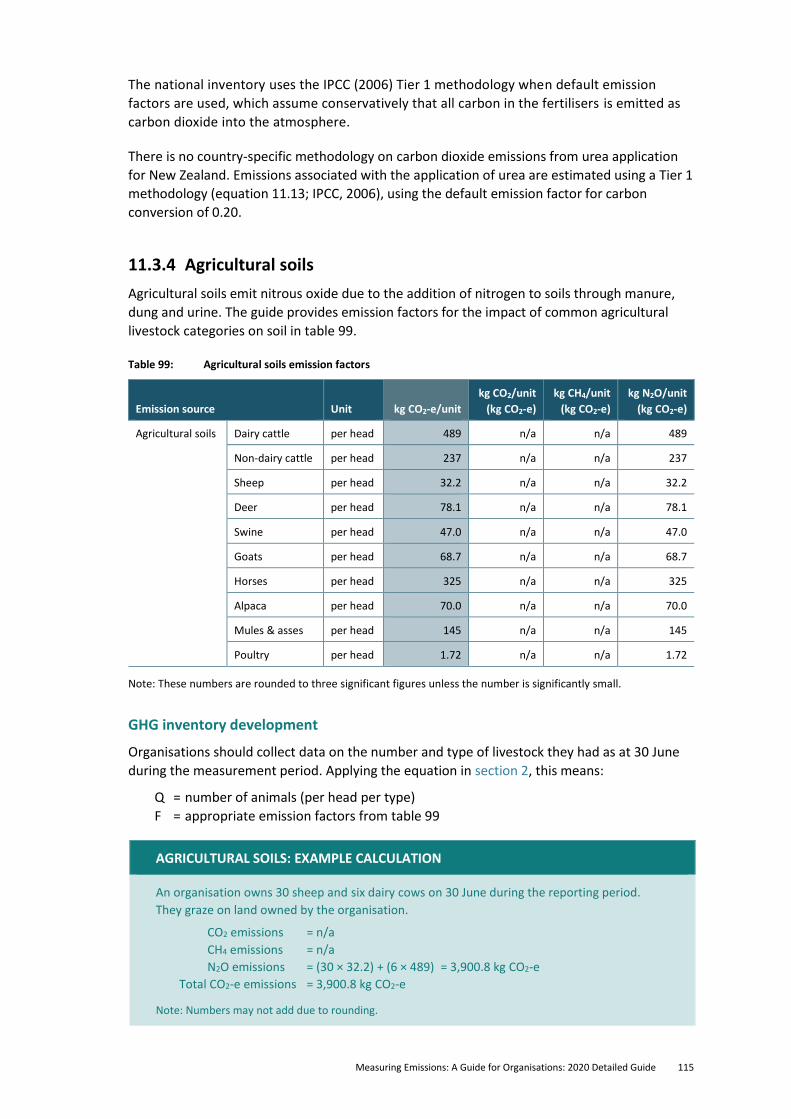
Measuring Emissions: A Guide for Organisations: 2020 Detailed Guide 115
The national inventory uses the IPCC (2006) Tier 1 methodology when default emission
factors are used, which assume conservatively that all carbon in the fertilisers is emitted as
carbon dioxide into the atmosphere.
There is no country-specific methodology on carbon dioxide emissions from urea application
for New Zealand. Emissions associated with the application of urea are estimated using a Tier 1
methodology (equation 11.13; IPCC, 2006), using the default emission factor for carbon
conversion of 0.20.
11.3.4 Agricultural soils
Agricultural soils emit nitrous oxide due to the addition of nitrogen to soils through manure,
dung and urine. The guide provides emission factors for the impact of common agricultural
livestock categories on soil in table 99.
Table 99: Agricultural soils emission factors
Emission source Unit kg CO2-e/unit
kg CO2/unit
(kg CO2-e)
kg CH4/unit
(kg CO2-e)
kg N2O/unit
(kg CO2-e)
Agricultural soils Dairy cattle per head 489 n/a n/a 489
Non-dairy cattle per head 237 n/a n/a 237
Sheep per head 32.2 n/a n/a 32.2
Deer per head 78.1 n/a n/a 78.1
Swine per head 47.0 n/a n/a 47.0
Goats per head 68.7 n/a n/a 68.7
Horses per head 325 n/a n/a 325
Alpaca per head 70.0 n/a n/a 70.0
Mules & asses per head 145 n/a n/a 145
Poultry per head 1.72 n/a n/a 1.72
Note: These numbers are rounded to three significant figures unless the number is significantly small.
GHG inventory development
Organisations should collect data on the number and type of livestock they had as at 30 June
during the measurement period. Applying the equation in section 2, this means:
Q = number of animals (per head per type)
F = appropriate emission factors from table 99
AGRICULTURAL SOILS: EXAMPLE CALCULATION
An organisation owns 30 sheep and six dairy cows on 30 June during the reporting period.
They graze on land owned by the organisation.
CO2 emissions = n/a
CH4 emissions = n/a
N2O emissions = (30 × 32.2) + (6 × 489) = 3,900.8 kg CO2-e
Total CO2-e emissions = 3,900.8 kg CO2-e
Note: Numbers may not add due to rounding.
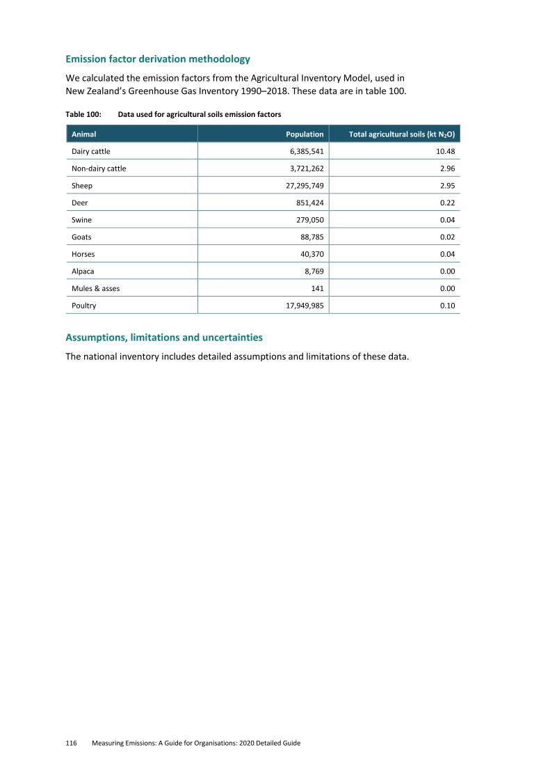
116 Measuring Emissions: A Guide for Organisations: 2020 Detailed Guide
Emission factor derivation methodology
We calculated the emission factors from the Agricultural Inventory Model, used in
New Zealand’s Greenhouse Gas Inventory 1990–2018. These data are in table 100.
Table 100: Data used for agricultural soils emission factors
Animal Population Total agricultural soils (kt N2O)
Dairy cattle 6,385,541 10.48
Non-dairy cattle 3,721,262 2.96
Sheep 27,295,749 2.95
Deer 851,424 0.22
Swine 279,050 0.04
Goats 88,785 0.02
Horses 40,370 0.04
Alpaca 8,769 0.00
Mules & asses 141 0.00
Poultry 17,949,985 0.10
Assumptions, limitations and uncertainties
The national inventory includes detailed assumptions and limitations of these data.
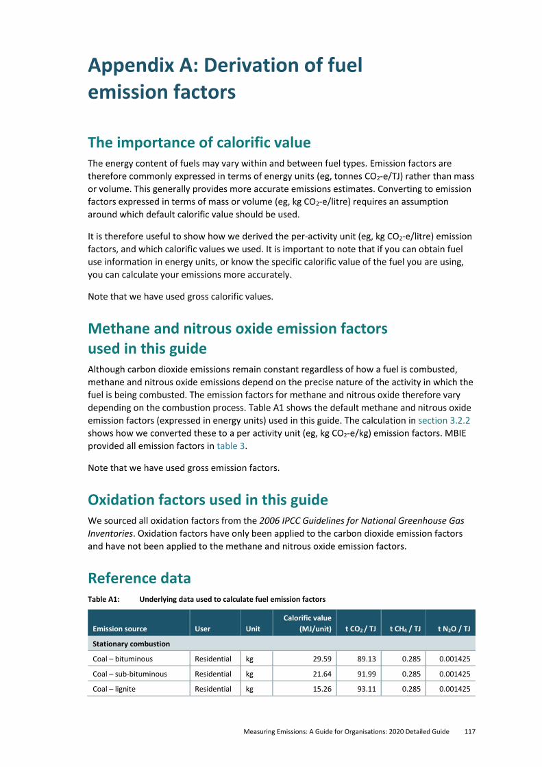
Measuring Emissions: A Guide for Organisations: 2020 Detailed Guide 117
Appendix A: Derivation of fuel emission factors
The importance of calorific value The energy content of fuels may vary within and between fuel types. Emission factors are
therefore commonly expressed in terms of energy units (eg, tonnes CO2-e/TJ) rather than mass
or volume. This generally provides more accurate emissions estimates. Converting to emission
factors expressed in terms of mass or volume (eg, kg CO2-e/litre) requires an assumption
around which default calorific value should be used.
It is therefore useful to show how we derived the per-activity unit (eg, kg CO2-e/litre) emission
factors, and which calorific values we used. It is important to note that if you can obtain fuel
use information in energy units, or know the specific calorific value of the fuel you are using,
you can calculate your emissions more accurately.
Note that we have used gross calorific values.
Methane and nitrous oxide emission factors used in this guide Although carbon dioxide emissions remain constant regardless of how a fuel is combusted,
methane and nitrous oxide emissions depend on the precise nature of the activity in which the
fuel is being combusted. The emission factors for methane and nitrous oxide therefore vary
depending on the combustion process. Table A1 shows the default methane and nitrous oxide
emission factors (expressed in energy units) used in this guide. The calculation in section 3.2.2
shows how we converted these to a per activity unit (eg, kg CO2-e/kg) emission factors. MBIE
provided all emission factors in table 3.
Note that we have used gross emission factors.
Oxidation factors used in this guide We sourced all oxidation factors from the 2006 IPCC Guidelines for National Greenhouse Gas
Inventories. Oxidation factors have only been applied to the carbon dioxide emission factors
and have not been applied to the methane and nitrous oxide emission factors.
Reference data Table A1: Underlying data used to calculate fuel emission factors
Emission source User Unit
Calorific value
(MJ/unit) t CO2 / TJ t CH4 / TJ t N2O / TJ
Stationary combustion
Coal – bituminous Residential kg 29.59 89.13 0.285 0.001425
Coal – sub-bituminous Residential kg 21.64 91.99 0.285 0.001425
Coal – lignite Residential kg 15.26 93.11 0.285 0.001425
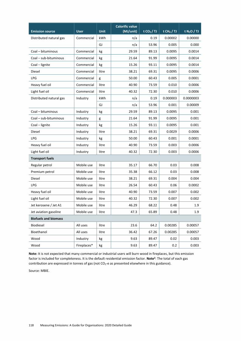
118 Measuring Emissions: A Guide for Organisations: 2020 Detailed Guide
Emission source User Unit
Calorific value
(MJ/unit) t CO2 / TJ t CH4 / TJ t N2O / TJ
Distributed natural gas Commercial kWh n/a 0.19 0.00002 0.00000
GJ n/a 53.96 0.005 0.000
Coal – bituminous Commercial kg 29.59 89.13 0.0095 0.0014
Coal – sub-bituminous Commercial kg 21.64 91.99 0.0095 0.0014
Coal – lignite Commercial kg 15.26 93.11 0.0095 0.0014
Diesel Commercial litre 38.21 69.31 0.0095 0.0006
LPG Commercial g 50.00 60.43 0.005 0.0001
Heavy fuel oil Commercial litre 40.90 73.59 0.010 0.0006
Light fuel oil Commercial litre 40.32 72.30 0.010 0.0006
Distributed natural gas Industry kWh n/a 0.19 0.000003 0.0000003
GJ n/a 53.96 0.001 0.00009
Coal – bituminous Industry kg 29.59 89.13 0.0095 0.001
Coal – sub-bituminous Industry g 21.64 91.99 0.0095 0.001
Coal – lignite Industry kg 15.26 93.11 0.0095 0.001
Diesel Industry litre 38.21 69.31 0.0029 0.0006
LPG Industry kg 50.00 60.43 0.001 0.0001
Heavy fuel oil Industry litre 40.90 73.59 0.003 0.0006
Light fuel oil Industry litre 40.32 72.30 0.003 0.0006
Transport fuels
Regular petrol Mobile use litre 35.17 66.70 0.03 0.008
Premium petrol Mobile use litre 35.38 66.12 0.03 0.008
Diesel Mobile use litre 38.21 69.31 0.004 0.004
LPG Mobile use litre 26.54 60.43 0.06 0.0002
Heavy fuel oil Mobile use litre 40.90 73.59 0.007 0.002
Light fuel oil Mobile use litre 40.32 72.30 0.007 0.002
Jet kerosene / Jet A1 Mobile use litre 46.29 68.22 0.48 1.9
Jet aviation gasoline Mobile use litre 47.3 65.89 0.48 1.9
Biofuels and biomass
Biodiesel All uses litre 23.6 64.2 0.00285 0.00057
Bioethanol All uses litre 36.42 67.26 0.00285 0.00057
Wood Industry kg 9.63 89.47 0.02 0.003
Wood Fireplaces* kg 9.63 89.47 0.2 0.003
Note: It is not expected that many commercial or industrial users will burn wood in fireplaces, but this emission
factor is included for completeness. It is the default residential emission factor. Note2: The total of each gas
contribution are expressed in tonnes of gas (not CO2-e as presented elsewhere in this guidance).
Source: MBIE.
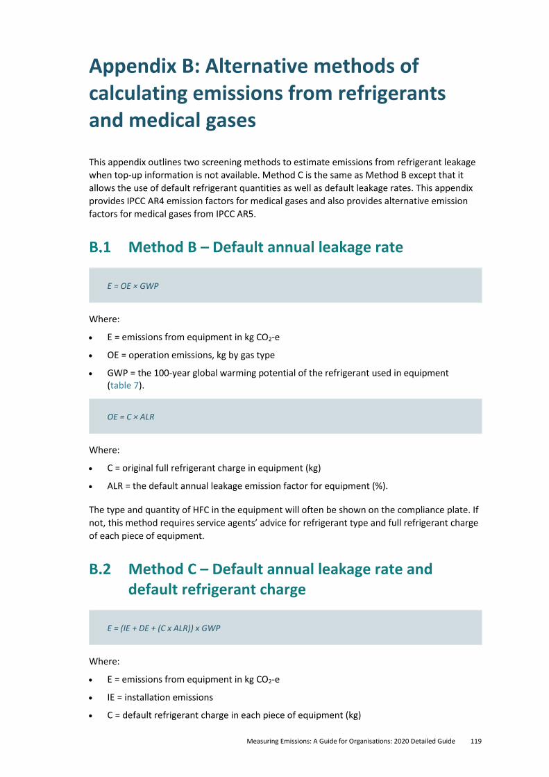
Measuring Emissions: A Guide for Organisations: 2020 Detailed Guide 119
Appendix B: Alternative methods of calculating emissions from refrigerants and medical gases
This appendix outlines two screening methods to estimate emissions from refrigerant leakage
when top-up information is not available. Method C is the same as Method B except that it
allows the use of default refrigerant quantities as well as default leakage rates. This appendix
provides IPCC AR4 emission factors for medical gases and also provides alternative emission
factors for medical gases from IPCC AR5.
Method B – Default annual leakage rate
E = OE × GWP
Where:
• E = emissions from equipment in kg CO2-e
• OE = operation emissions, kg by gas type
• GWP = the 100-year global warming potential of the refrigerant used in equipment (table 7).
OE = C × ALR
Where:
• C = original full refrigerant charge in equipment (kg)
• ALR = the default annual leakage emission factor for equipment (%).
The type and quantity of HFC in the equipment will often be shown on the compliance plate. If
not, this method requires service agents’ advice for refrigerant type and full refrigerant charge
of each piece of equipment.
B.2 Method C – Default annual leakage rate and default refrigerant charge
E = (IE + DE + (C x ALR)) x GWP
Where:
• E = emissions from equipment in kg CO2-e
• IE = installation emissions
• C = default refrigerant charge in each piece of equipment (kg)
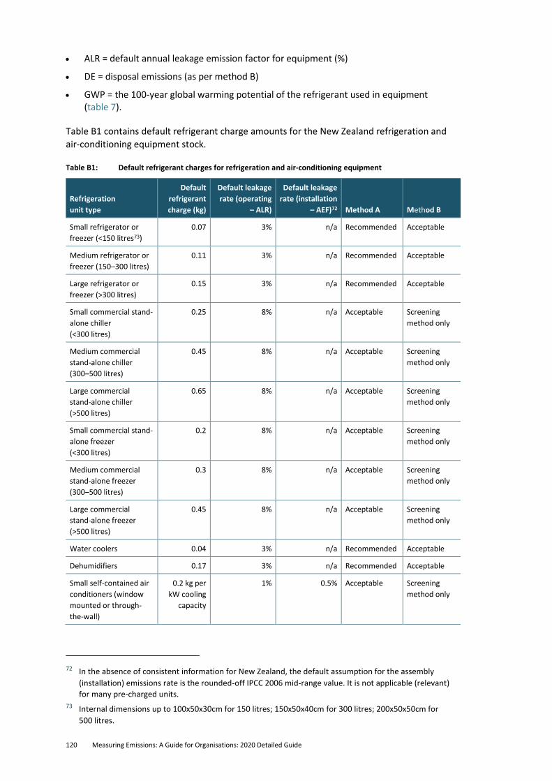
120 Measuring Emissions: A Guide for Organisations: 2020 Detailed Guide
• ALR = default annual leakage emission factor for equipment (%)
• DE = disposal emissions (as per method B)
• GWP = the 100-year global warming potential of the refrigerant used in equipment (table 7).
Table B1 contains default refrigerant charge amounts for the New Zealand refrigeration and
air-conditioning equipment stock.
Table B1: Default refrigerant charges for refrigeration and air-conditioning equipment
Refrigeration
unit type
Default
refrigerant
charge (kg)
Default leakage
rate (operating
– ALR)
Default leakage
rate (installation
– AEF)72 Method A Method B
Small refrigerator or
freezer (<150 litres73)
0.07 3% n/a Recommended Acceptable
Medium refrigerator or
freezer (150–300 litres)
0.11 3% n/a Recommended Acceptable
Large refrigerator or
freezer (>300 litres)
0.15 3% n/a Recommended Acceptable
Small commercial stand-
alone chiller
(<300 litres)
0.25 8% n/a Acceptable Screening
method only
Medium commercial
stand-alone chiller
(300–500 litres)
0.45 8% n/a Acceptable Screening
method only
Large commercial
stand-alone chiller
(>500 litres)
0.65 8% n/a Acceptable Screening
method only
Small commercial stand-
alone freezer
(<300 litres)
0.2 8% n/a Acceptable Screening
method only
Medium commercial
stand-alone freezer
(300–500 litres)
0.3 8% n/a Acceptable Screening
method only
Large commercial
stand-alone freezer
(>500 litres)
0.45 8% n/a Acceptable Screening
method only
Water coolers 0.04 3% n/a Recommended Acceptable
Dehumidifiers 0.17 3% n/a Recommended Acceptable
Small self-contained air
conditioners (window
mounted or through-
the-wall)
0.2 kg per
kW cooling
capacity
1% 0.5% Acceptable Screening
method only
72 In the absence of consistent information for New Zealand, the default assumption for the assembly
(installation) emissions rate is the rounded-off IPCC 2006 mid-range value. It is not applicable (relevant)
for many pre-charged units.
73 Internal dimensions up to 100x50x30cm for 150 litres; 150x50x40cm for 300 litres; 200x50x50cm for
500 litres.
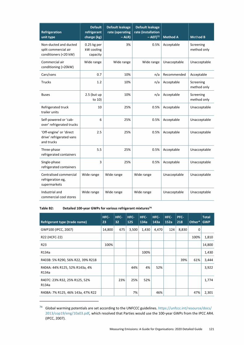
Measuring Emissions: A Guide for Organisations: 2020 Detailed Guide 121
Refrigeration
unit type
Default
refrigerant
charge (kg)
Default leakage
rate (operating
– ALR)
Default leakage
rate (installation
– AEF)72 Method A Method B
Non-ducted and ducted
split commercial air
conditioners (<20 kW)
0.25 kg per
kW cooling
capacity
3% 0.5% Acceptable Screening
method only
Commercial air
conditioning (>20kW)
Wide range Wide range Wide range Unacceptable Unacceptable
Cars/vans 0.7 10% n/a Recommended Acceptable
Trucks 1.2 10% n/a Acceptable Screening
method only
Buses 2.5 (but up
to 10)
10% n/a Acceptable Screening
method only
Refrigerated truck
trailer units
10 25% 0.5% Acceptable Unacceptable
Self-powered or ‘cab-
over’ refrigerated trucks
6 25% 0.5% Acceptable Unacceptable
‘Off-engine’ or ‘direct
drive’ refrigerated vans
and trucks
2.5 25% 0.5% Acceptable Unacceptable
Three-phase
refrigerated containers
5.5 25% 0.5% Acceptable Unacceptable
Single-phase
refrigerated containers
3 25% 0.5% Acceptable Unacceptable
Centralised commercial
refrigeration eg,
supermarkets
Wide range Wide range Wide range Unacceptable Unacceptable
Industrial and
commercial cool stores
Wide range Wide range Wide range Unacceptable Unacceptable
Table B2: Detailed 100-year GWPs for various refrigerant mixtures74
Refrigerant type (trade name)
HFC-
23
HFC-
32
HFC-
125
HFC-
134a
HFC-
143a
HFC-
152a
PFC-
218 Other*
Total
GWP
GWP100 (IPCC, 2007) 14,800 675 3,500 1,430 4,470 124 8,830 0
R22 (HCFC-22) 100% 1,810
R23 100% 14,800
R134a 100% 1,430
R403B: 5% R290, 56% R22, 39% R218 39% 61% 3,444
R404A: 44% R125, 52% R143a, 4%
R134a
44% 4% 52% 3,922
R407C: 23% R32, 25% R125, 52%
R134a
23% 25% 52% 1,774
R408A: 7% R125, 46% 143a, 47% R22 7% 46% 47% 2,301
74 Global warming potentials are set according to the UNFCCC guidelines. https://unfccc.int/resource/docs/
2013/cop19/eng/10a03.pdf, which resolved that Parties would use the 100-year GWPs from the IPCC AR4.
(IPCC, 2007).
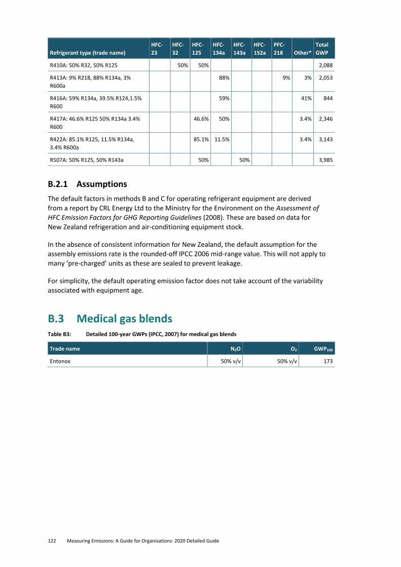
122 Measuring Emissions: A Guide for Organisations: 2020 Detailed Guide
Refrigerant type (trade name)
HFC-
23
HFC-
32
HFC-
125
HFC-
134a
HFC-
143a
HFC-
152a
PFC-
218 Other*
Total
GWP
R410A: 50% R32, 50% R125 50% 50% 2,088
R413A: 9% R218, 88% R134a, 3%
R600a
88% 9% 3% 2,053
R416A: 59% R134a, 39.5% R124,1.5%
R600
59% 41% 844
R417A: 46.6% R125 50% R134a 3.4%
R600
46.6% 50% 3.4% 2,346
R422A: 85.1% R125, 11.5% R134a,
3.4% R600a
85.1% 11.5% 3.4% 3,143
R507A: 50% R125, 50% R143a 50% 50% 3,985
B.2.1 Assumptions
The default factors in methods B and C for operating refrigerant equipment are derived
from a report by CRL Energy Ltd to the Ministry for the Environment on the Assessment of
HFC Emission Factors for GHG Reporting Guidelines (2008). These are based on data for
New Zealand refrigeration and air-conditioning equipment stock.
In the absence of consistent information for New Zealand, the default assumption for the
assembly emissions rate is the rounded-off IPCC 2006 mid-range value. This will not apply to
many ‘pre-charged’ units as these are sealed to prevent leakage.
For simplicity, the default operating emission factor does not take account of the variability
associated with equipment age.
B.3 Medical gas blends Table B3: Detailed 100-year GWPs (IPCC, 2007) for medical gas blends
Trade name N2O O2 GWP100
Entonox 50% v/v 50% v/v 173
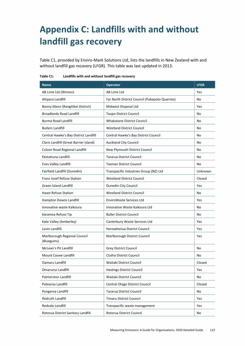
Measuring Emissions: A Guide for Organisations: 2020 Detailed Guide 123
Appendix C: Landfills with and without landfill gas recovery
Table C1, provided by Enviro-Mark Solutions Ltd, lists the landfills in New Zealand with and
without landfill gas recovery (LFGR). This table was last updated in 2013.
Table C1: Landfills with and without landfill gas recovery
Name Operator LFGR
AB Lime Ltd (Winton) AB Lime Ltd Yes
Ahipara Landfill Far North District Council (Pukepoto Quarries) No
Bonny Glenn (Rangitikei District) Midwest Disposal Ltd Yes
Broadlands Road Landfill Taupo District Council No
Burma Road Landfill Whakatane District Council No
Butlers Landfill Westland District Council No
Central Hawke’s Bay District Landfill Central Hawke’s Bay District Council No
Claris Landfill (Great Barrier Island) Auckland City Council No
Colson Road Regional Landfill New Plymouth District Council No
Eketahuna Landfill Tararua District Council No
Eves Valley Landfill Tasman District Council No
Fairfield Landfill (Dunedin) Transpacific Industries Group (NZ) Ltd Unknown
Franz Josef Refuse Station Westland District Council Closed
Green Island Landfill Dunedin City Council Yes
Haast Refuse Station Westland District Council No
Hampton Downs Landfill EnviroWaste Services Ltd Yes
Innovative waste Kaikoura Innovative Waste Kaikoura Ltd No
Karamea Refuse Tip Buller District Council No
Kate Valley (Amberley) Canterbury Waste Services Ltd Yes
Levin Landfill Horowhenua District Council Yes
Marlborough Regional Council
(Bluegums)
Marlborough District Council Yes
McLean’s Pit Landfill Grey District Council No
Mount Cooee Landfill Clutha District Council No
Oamaru Landfill Waitaki District Council Closed
Omarunui Landfill Hastings District Council Yes
Palmerston Landfill Waitaki District Council No
Patearoa Landfill Central Otago District Council Closed
Pongaroa Landfill Tararua District Council No
Redruth Landfill Timaru District Council Yes
Redvale Landfill Transpacific waste management Yes
Rotorua District Sanitary Landfill Rotorua District Council No
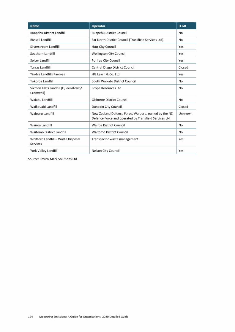
124 Measuring Emissions: A Guide for Organisations: 2020 Detailed Guide
Name Operator LFGR
Ruapehu District Landfill Ruapehu District Council No
Russell Landfill Far North District Council (Transfield Services Ltd) No
Silverstream Landfill Hutt City Council Yes
Southern Landfill Wellington City Council Yes
Spicer Landfill Porirua City Council Yes
Tarras Landfill Central Otago District Council Closed
Tirohia Landfill (Paeroa) HG Leach & Co. Ltd Yes
Tokoroa Landfill South Waikato District Council No
Victoria Flats Landfill (Queenstown/
Cromwell)
Scope Resources Ltd No
Waiapu Landfill Gisborne District Council No
Waikouaiti Landfill Dunedin City Council Closed
Waiouru Landfill New Zealand Defence Force, Waiouru, owned by the NZ
Defence Force and operated by Transfield Services Ltd
Unknown
Wairoa Landfill Wairoa District Council No
Waitomo District Landfill Waitomo District Council No
Whitford Landfill – Waste Disposal
Services
Transpacific waste management Yes
York Valley Landfill Nelson City Council Yes
Source: Enviro-Mark Solutions Ltd
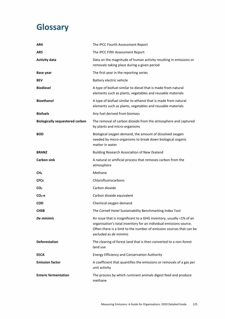
Measuring Emissions: A Guide for Organisations: 2020 Detailed Guide 125
Glossary
AR4 The IPCC Fourth Assessment Report
AR5 The IPCC Fifth Assessment Report
Activity data Data on the magnitude of human activity resulting in emissions or
removals taking place during a given period
Base year The first year in the reporting series
BEV Battery electric vehicle
Biodiesel A type of biofuel similar to diesel that is made from natural
elements such as plants, vegetables and reusable materials
Bioethanol A type of biofuel similar to ethanol that is made from natural
elements such as plants, vegetables and reusable materials
Biofuels Any fuel derived from biomass
Biologically sequestered carbon The removal of carbon dioxide from the atmosphere and captured
by plants and micro-organisms
BOD Biological oxygen demand, the amount of dissolved oxygen
needed by micro-organisms to break down biological organic
matter in water
BRANZ Building Research Association of New Zealand
Carbon sink A natural or artificial process that removes carbon from the
atmosphere
CH4 Methane
CFCs Chlorofluorocarbons
CO2 Carbon dioxide
CO2-e Carbon dioxide equivalent
COD Chemical oxygen demand
CHSB The Cornell Hotel Sustainability Benchmarking Index Tool
De minimis An issue that is insignificant to a GHG inventory, usually <1% of an
organisation’s total inventory for an individual emissions source.
Often there is a limit to the number of emission sources that can be
excluded as de minimis
Deforestation The clearing of forest land that is then converted to a non-forest
land use
EECA Energy Efficiency and Conservation Authority
Emission factor A coefficient that quantifies the emissions or removals of a gas per
unit activity
Enteric fermentation The process by which ruminant animals digest feed and produce
methane
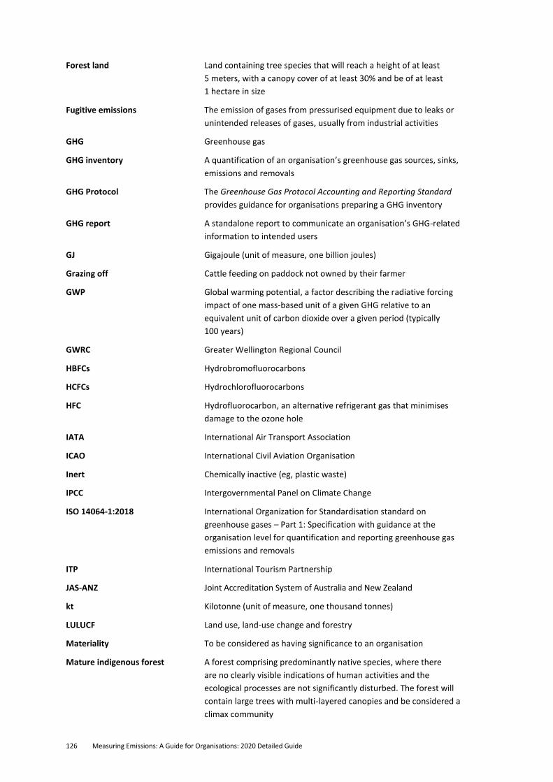
126 Measuring Emissions: A Guide for Organisations: 2020 Detailed Guide
Forest land Land containing tree species that will reach a height of at least
5 meters, with a canopy cover of at least 30% and be of at least
1 hectare in size
Fugitive emissions The emission of gases from pressurised equipment due to leaks or
unintended releases of gases, usually from industrial activities
GHG Greenhouse gas
GHG inventory A quantification of an organisation’s greenhouse gas sources, sinks,
emissions and removals
GHG Protocol The Greenhouse Gas Protocol Accounting and Reporting Standard
provides guidance for organisations preparing a GHG inventory
GHG report A standalone report to communicate an organisation’s GHG-related
information to intended users
GJ Gigajoule (unit of measure, one billion joules)
Grazing off Cattle feeding on paddock not owned by their farmer
GWP Global warming potential, a factor describing the radiative forcing
impact of one mass-based unit of a given GHG relative to an
equivalent unit of carbon dioxide over a given period (typically
100 years)
GWRC Greater Wellington Regional Council
HBFCs Hydrobromofluorocarbons
HCFCs Hydrochlorofluorocarbons
HFC Hydrofluorocarbon, an alternative refrigerant gas that minimises
damage to the ozone hole
IATA International Air Transport Association
ICAO International Civil Aviation Organisation
Inert Chemically inactive (eg, plastic waste)
IPCC Intergovernmental Panel on Climate Change
ISO 14064-1:2018 International Organization for Standardisation standard on
greenhouse gases – Part 1: Specification with guidance at the
organisation level for quantification and reporting greenhouse gas
emissions and removals
ITP International Tourism Partnership
JAS-ANZ Joint Accreditation System of Australia and New Zealand
kt Kilotonne (unit of measure, one thousand tonnes)
LULUCF Land use, land-use change and forestry
Materiality To be considered as having significance to an organisation
Mature indigenous forest A forest comprising predominantly native species, where there
are no clearly visible indications of human activities and the
ecological processes are not significantly disturbed. The forest will
contain large trees with multi-layered canopies and be considered a
climax community
Measuring Emissions: A Guide for Organisations: 2020 Detailed Guide 127
MBIE Ministry of Business, Innovation and Employment
MfE Ministry for the Environment
MoT Ministry of Transport
MPI Ministry of Primary Industries
Municipal landfill Landfill that accepts household waste as well as other wastes
National inventory New Zealand’s Greenhouse Gas Inventory
NDC Nationally determined contributions under the Paris Agreement
NF3 Nitrogen trifluoride
N2O Nitrous oxide
NZ ETS New Zealand Emissions Trading Scheme
NZTA Waka Kotahi New Zealand Transport Agency
ODS Ozone-depleting substances
Organisational boundary The boundary of the organisation as it applies to measurement of
GHG emissions. This typically aligns with legal and/or organisational
structure; a financial boundary must be drawn within this too
OVERSEER A New Zealand software platform that enables farmers and
growers to estimate and improve nutrient use on farms
PFC Perfluorocarbon
PHEV Plug-in hybrid electric vehicle
pkm Passenger-kilometre (unit of measure for transport)
Radiative forcing The difference between solar energy absorbed by the Earth and
that radiated back to space. Human activity has impacts which alter
radiative forcing
Refrigerants A substance or mixture used in a heat pump and refrigeration cycle
Removals Withdrawal of a GHG from the atmosphere by GHG sinks
Reporting boundary The emission sources included within an organisation’s operations,
including direct and indirect emission sources. It includes choosing
which indirect emission sources to report
Reticulated gas A piped gas system to deliver a gas such as LPG or natural gas to
a consumer
Scope Emission sources are categorised by Scope to manage risks and
impacts of double counting. There are three scopes in greenhouse
gas reporting: Scope 1 (direct emissions), Scope 2 (energy indirect
emissions) and Scope 3 (other indirect emissions)
SF6 Sulphur hexafluoride
Stationary combustion fuel Fuel used in an unmoving engine eg, a power plant or boiler
TFCD Task Force on Climate-related Financial Disclosures
tkm Tonne-kilometre (unit of measure for freight)

128 Measuring Emissions: A Guide for Organisations: 2020 Detailed Guide
Unique emission factor A value given to an activity based on how emissions intensive it is.
Experienced professionals must verify a unique emission factor. See
Climate Change (Unique Emission Factors) Regulations 2009 for
further information
Uplift factor Applied to take into account the combined ‘real-world’ effects on
fuel consumption (such as non-direct flight paths)
VFEM The 2019 Vehicle Fleet Emissions Model supplied by the Ministry of
Transport