Embed Size (px)
Citation preview
arX
iv:0
706.
4165
v3 [
hep-
ph]
16
Jan
2008
DESY 07-097
June 2007
Probing New Physics in the Neutrinoless Double Beta DecayUsing Electron Angular Correlation
A. Ali 1
Deutsches Elektronen-Synchrotron, DESY, 22607 Hamburg, Germany
A.V. Borisov2 , D.V. Zhuridov3
Faculty of Physics, Moscow State University, 119991 Moscow, Russia
Abstract
The angular correlation of the electrons emitted in the neutrinoless double beta decay (0ν2β) ispresented using a general Lorentz invariant effective Lagrangian for the leptonic and hadronic chargedweak currents. We show that the coefficient K in the angular correlation dΓ/d cos θ ∝ (1 − K cos θ) isessentially independent of the nuclear matrix element models and present its numerical values for the fivenuclei of interest (76Ge, 82Se, 100Mo, 130Te, and 136Xe), assuming that the 0ν2β-decays in these nucleiare induced solely by a light Majorana neutrino, νM . This coefficient varies between K = 0.81 (for the76Ge nucleus) and K = 0.88 (for the 82Se and 100Mo nuclei), calculated taking into account the effectsfrom the nucleon recoil, the S and P -waves for the outgoing electrons and the electron mass. Deviationof K from its values derived here would indicate the presence of New Physics (NP) in addition to a lightMajorana neutrino, and we work out the angular coefficients in several νM +NP scenarios for the 76Genucleus. As an illustration of the correlations among the 0ν2β observables (half-life T1/2, the coefficientK, and the effective Majorana neutrino mass |〈m〉|) and the parameters of the underlying NP model, weanalyze the left-right symmetric models, taking into account current phenomenological bounds on theright-handed WR-boson mass and the left-right mixing parameter ζ.
1e-mail: [email protected]: [email protected]: [email protected]
1
1 Introduction
It is now established beyond any doubt that the observed neutrinos have tiny but non-zero masses and theymix with each other, with both of these features following from the observation of the atmospheric andsolar neutrino oscillations and from the long baseline neutrino oscillation experiments [1]. Theoretically, itis largely anticipated that the neutrinos are Majorana particles. Experimental evidence for the neutrinolessdouble beta decay (0ν2β) would deliver a conclusive confirmation of the Majorana nature of neutrinos,establishing the existence of physics beyond the standard model. This is the overriding interest in carryingout these experiments and in the related phenomenology [2].
We recall that 0ν2β-decays are forbidden in the standard model (SM) by lepton number (LN) conser-vation, which is a consequence of the renormalizability of the SM. However, being the low energy limit ofa more general theory, an extended version of the SM could contain nonrenormalizable terms (tiny to becompatible with experiments), in particular, terms that violate LN and allow the 0ν2β decay. Probablemechanisms of LN violation may include exchanges by: Majorana neutrinos νM s [3, 4, 5] (the preferredmechanism after the observation of neutrino oscillations [1]), SUSY particles [6, 7, 8, 9, 10, 11], scalar bilin-ears (SBs) [12], e.g. doubly charged dileptons (the component ξ−− of the SU(2)L triplet Higgs scalar etc.),leptoquarks (LQs) [13], right-handed WR bosons [5, 14] etc. From these particles light νs are much lighterthan the electron and others are much heavier than the proton. Therefore, there are two possible classes ofmechanisms for the 0ν2β decay. With the light νs in the intermediate state the mechanism is called longrange and otherwise it is referred to as the short range mechanism. For both these classes, the separationof the lepton physics from the hadron physics takes place [15], which simplifies calculations. According tothe Schechter–Valle theorem [16], any mechanism inducing the 0ν2β decay produces an effective Majoranamass for the neutrino, which must therefore contribute to this decay. These various contributions will haveto be disentangled to extract information from the 0ν2β decay on the characteristics of the sources of LNviolation, in particular, on the neutrino masses and mixing. Measurements of the neutrinoless double betadecay in different nuclei will help in determining the underlying physics mechanism [17, 18].
Our aim in this paper is to examine the possibility to discriminate among the various possible mechanismscontributing to the 0ν2β-decays using the information on the angular correlation of the final electrons inthe process Ni(A,Z) → Nf(A,Z + 2) + e− + e−. A preliminary study along these lines was published byus in 2006 [19], with admittedly simplified treatment neglecting the nucleon recoil and the P -wave effectsin the outgoing electron wave function. We rectify these shortcomings and provide in this paper a detailedaccount of the improved treatment. Restricting ourselves to the long-range mechanism, treating the electronsrelativistically but with non-relativistic nucleons, we derive the angular correlation between the electronsusing the general Lorentz invariant effective Lagrangian involving the leptonic and hadronic charged weakcurrents. Generally, this angular correlation can be expressed as dΓ/d cos θ ∼ 1 − K cos θ, where θ is theangle between the electron momenta in the rest frame of the parent nucleus. Expressing K = B/A, with−1 < K < 1, we derive the analytic expressions for A and B for the effective Lagrangian characterized bythe coefficients ǫβαi encoding the standard, (V −A)⊗ (V −A), and new physics contributions (see Eq. (1)).Essential steps of these derivations are presented in section 2. The analytic expressions derived here confirmthe earlier detailed derivations by Doi et al. [5], and we specify where the treatment presented here transcendsthe earlier work. Specific cases are relegated to Appendix A (for the decays involving scalar nonstandardterms), Appendix B (for the vector nonstandard terms), and Appendix C (for the tensor nonstandard terms).We hope to return to the discussion of including the short-range mechanism, neglected in this paper, in futurework.
Numerical analysis of the electron angular correlation is presented in section 3, and the coefficient K forthe various underlying mechanisms in 0ν2β-decays are worked out. In particular, numerical values of K forthe five nuclei of current experimental interest: 76Ge, 82Se, 100Mo, 130Te, and 136Xe are presented for thelight Majorana neutrino νM case. Their values range from K = 0.81 (for the 76Ge nucleus) and K = 0.88(for the 82Se and 100Mo nuclei). To study the uncertainty in the nuclear matrix elements, we have employedthe so-called QRPA model with and without the p-n pairing for the 76Ge nucleus [20], and a more modernQRPA model, fixing the particle-particle pairing strength [21]. While the uncertainty due to the nuclearmatrix element model is quite marked for T1/2 in some cases, we show that it is rather modest for K, notexceeding 10% for the models discussed here. For the νM + NP scenarios, we remark that the nonstandard
2
coefficients ǫV−AV∓A, ǫ
TL
TR, and ǫTR
TLdo not change the value of the angular coefficient K. The contribution of the
scalar nonstandard term from the ǫS+PS∓P coefficients is found to be numerically small. So, what concerns the
angular correlation, we have essentially three distinct scenarios: (i) Standard (νM ), (ii) R-parity violatingSUSY (νM + ǫTR
TR), and (iii) left-right-symmetric models (νM + ǫV∓A
V+A). Numerical analysis of the coefficient
K in the extended νM +NP scenario is carried out for the decay of the 76Ge nucleus using the nuclear matrixelement model already specified.
We take a closer look at the underlying physics behind the coefficients ǫV∓AV∓A in section 4. These coefficients
appear in the context of the left-right symmetric models which are theoretically well motivated [22]. Also,the corresponding nuclear matrix elements are available in the literature. Making use of them, we work outthe correlations among the angular coefficient K, the half-life T1/2 and either the mass of the right-handedWR boson, mWR , or the W boson’s mixing angle ζ, taking into account the current bounds on the variousparameters. Results are presented in Figs. 1 – 4. The differential distribution dΓ/d cos θ for the 0ν2β decayof the 76Ge nucleus is shown in Fig. 5 for some representative values of |〈m〉| for mWR = 1, 1.5 TeV andfor an infinitely heavy mWR . It is seen that the effect of the right-handed WR-boson is more marked in theangular correlation for smaller values of |〈m〉|.
2 Angular correlation for the long range mechanism of 0ν2β decay
2.1 General effective Lagrangian
For the decay mediated by light νMs, the most general effective Lagrangian is the Lorentz invariant combi-nation of the leptonic jα and the hadronic Jα currents of definite tensor structure and chirality [23, 24]
L =GFVud√
2[(Uei + ǫV−A
V−A,i)jµiV −AJ
+V−A,µ +
∑
α,β
′
ǫβαijiβJ
+α +H.c.] , (1)
where the hadronic and leptonic currents are defined as: J+α = uOαd and jiβ = eOβνi; the leptonic currents
contain neutrino mass eigenstates and the index i runs over the light eigenstates. Here and thereafter, asummation over the repeated indices is assumed; α,β=V ∓A,S∓P ,TL,R (OTρ = 2σµνPρ, σ
µν = i2 [γ
µ, γν ],Pρ = (1∓γ5)/2 is the projector, ρ = L, R); the prime indicates the summation over all the Lorentz invariantcontributions, except for α = β = V − A, Uei is the PMNS mixing matrix [25] and Vud is the CKMmatrix element [1]. Note that in Eq. (1) the currents have been scaled relative to the strength of the usual
V − A interaction with GF being the Fermi coupling constant. The coefficients ǫβαi encode new physics,parametrizing deviations of the Lagrangian from the standard V −A current-current form and mixing of thenon-SM neutrinos.
In discussing the extension of the SM for the 0ν2β decay, Ref. [5] considered explicitly only nonstandardterms with
ǫV−AV+A,i = κ
g′VgVU ′ei, ǫV+A
V−A,i = ηV ′ei, ǫV+A
V+A,i = λg′VgVVei . (2)
Implicitly, also the contributions encoded by the coefficients ǫV−AV−A,i are discussed arising from the non-SM
contribution to Uei in SU(2)L×SU(2)R×U(1) models with mirror leptons (see Ref. [5], Eq. (A.2.17)). HereV , U ′ and V ′ are the 3 × 3 blocks of mixing matrices for non-SM neutrinos, e.g., for the usual SU(2)L ×SU(2)R × U(1) model V describes the lepton mixing for neutrinos from right-handed lepton doublets; forSU(2)L × SU(2)R × U(1) model with mirror leptons [26] U ′ (V ′) describes the lepton mixing for mirrorleft(right)-handed neutrinos [5] etc. The form factors gV and g′V are expressed through the mixing anglesfor left- and right-handed quarks. Thus, gV = cos θC = Vud and g′V = eiδ cos θ′C , with θC being the Cabibboangle, θ′C is its right-handed mixing analogoue, and the CP violating phase δ arises in these models due toboth the mixing of right-handed quarks and the mixing of left- and right-handed gauge bosons (see Ref. [5],Eq. (3.1.11)). The parameters κ, η, and λ characterize the strength of nonstandard effects. Below, we givesome illustrative examples relating the coefficients ǫV −A
V −A,i, ǫV+AV±A,i and the particle masses, couplings and the
mixing parameters in the underlying theoretical models.
In the R-parity-violating (RPV) SUSY accompanying the neutrino exchange mechanism [6, 7, 8, 9, 10, 11],SUSY particles (sleptons, squarks) are present in one of the two effective 4-fermion vertices. (The other vertex
3
contains the usual WL boson.) The nonzero parameters are
ǫV−AV−A,i =
1
2ηn1(q)RRUni, ǫS−P
S+P,i = 2ηn1(l)LLUni,
ǫS+PS+P,i = −1
4
(
ηn1(q)LR − 4ηn1(l)LR
)
U∗ni, ǫ
TR
TR,i =1
8ηn1(q)LRU
∗ni, (3)
where the index n runs over e, µ, τ (1, 2, 3), and the RPV Minimal Supersymmetric Model (MSSM)parameters ηs depend on the couplings of the RPV MSSM superpotential, the masses of the squarks andthe sleptons, the mixings among the squarks and among the sleptons. Concentrating on the dominantcontributions ǫS+P
S+P,i and ǫTR
TR,i (as the others are helicity-suppressed), one can express ηn1(q)LR and ηn1(l)LR as
follows [10]
ηn1(q)LR =∑
k
λ′11kλ′nk1
2√2GF
sin 2θd(k)
(
1
m2d1(k)
− 1
m2d2(k)
)
,
ηn1(l)LR =∑
k
λ′k11λn1k
2√2GF
sin 2θe(k)
(
1
m2e1(k)
− 1
m2e2(k)
)
, (4)
where k is the generation index, θd(k) and θe(k) are the squark and slepton mixing angles, respectively, mf1
and mf2are the sfermion mass eigenvalues, and λijk and λ′ijk are the RPV-couplings in the superpotential.
For the mechanism with LQs in one of the effective vertices [13], the nonzero coefficients are
ǫS+PS−P = −
√2
4GF
ǫVM2
V
, ǫS+PS+P = −
√2
4GF
ǫSM2
S
,
ǫV+AV−A = − 1
2GF
(
α(L)S
M2S
+α(L)V
M2V
)
, ǫV+AV+A = −
√2
4GF
(
α(R)S
M2S
+α(R)V
M2V
)
, (5)
whereǫβα = Ueiǫ
βαi, (6)
the parameters ǫS(V ), α(L)S(V ), and α
(R)S(V ) depend on the couplings of the renormalizable LQ-quark-lepton
interactions consistent with the SM gauge symmetry, the mixing parameters and the common mass scaleMS(V ) of the scalar (vector) LQs [27].
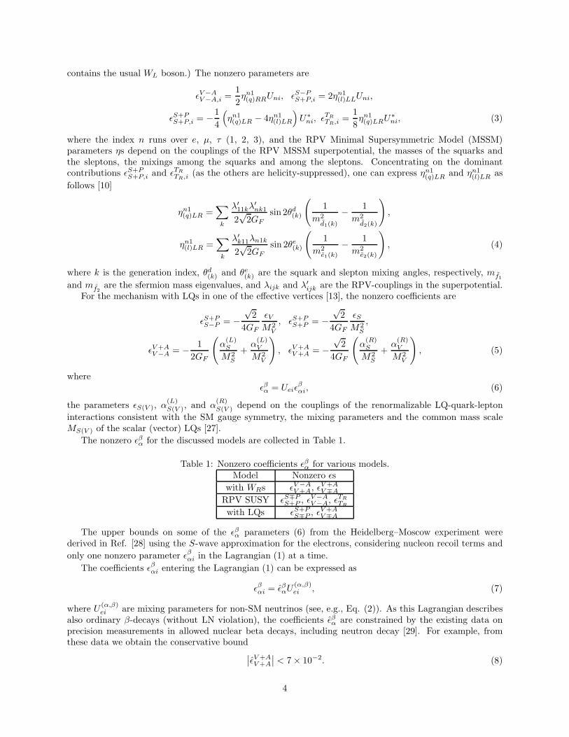
The nonzero ǫβα for the discussed models are collected in Table 1.
Table 1: Nonzero coefficients ǫβα for various models.Model Nonzero ǫs
with WRs ǫV −AV +A, ǫ
V +AV ∓A
RPV SUSY ǫS∓PS+P , ǫ
V−AV−A, ǫ
TR
TR
with LQs ǫS+PS∓P , ǫ
V+AV∓A
The upper bounds on some of the ǫβα parameters (6) from the Heidelberg–Moscow experiment werederived in Ref. [28] using the S-wave approximation for the electrons, considering nucleon recoil terms and
only one nonzero parameter ǫβαi in the Lagrangian (1) at a time.
The coefficients ǫβαi entering the Lagrangian (1) can be expressed as
ǫβαi = ǫβαU(α,β)ei , (7)
where U(α,β)ei are mixing parameters for non-SM neutrinos (see, e.g., Eq. (2)). As this Lagrangian describes
also ordinary β-decays (without LN violation), the coefficients ǫβα are constrained by the existing data onprecision measurements in allowed nuclear beta decays, including neutron decay [29]. For example, fromthese data we obtain the conservative bound
∣
∣ǫV +AV +A
∣
∣ < 7× 10⁻². (8)
4
From Eqs. (6), (7), (8) and the bound∣
∣ǫV+AV+A
∣
∣ < 7.9 × 10⁻⁷ (see section 3.2) we can assume that thenonstandard mixing is small:
|UeiVei| . 10−5, Vei = U(V+A,V+A)ei . (9)
2.2 Methods and approximations
We have calculated the leading order in the Fermi constant taking into account the leading contribution ofthe parameters ǫβα to the decay matrix elements using the approximation of the relativistic electrons andnon-relativistic nucleons. The wavefunction of an electron with the asymptotic momentum p and the spinprojection s can be expanded in terms of spherical waves as [5, 30]
eps(r) = eS1/2ps (r) + e
P1/2ps (r) + . . . (10)
We take into account the S1/2 and the P1/2 waves for the outgoing electrons:
eS1/2ps (r) =
(
g−1χs
f1σ · pχs
)
, (11)
eP1/2ps (r) = i
(
g1σ · rσ · pχs
−f−1σ · rχs
)
, (12)
with r = r/r, p = p/p and the two component spinor χs. We use the approximate radial wave functions [5]
(
g−1
f1
)
= A∓1
[
1− 1
6(pr)2
]
, (13)
(pr)2 =
(
3
2αZ
)2( r
R
)2
+ 3αZr
Rεr + (pr)2, (14)
(
g1f−1
)
= ±A∓1ξ±(ε)r
R, ξ± =
1
2αZ +
1
3(ε±me)R, (15)
including the finite de Broglie wave length correction (FBWC) for the S1/2 wave. Here R is the nuclear
radius, ε is the electron energy and α is the fine structure constant. For the normalization constants A±1
we use the approximate Eq. (45) (see below).The nucleon matrix elements of the color singlet quark currents are [8, 31, 32, 33]
〈P (k′)|u(1∓ γ5)d|N(k)〉 = ψ(k′)[
F(3)S (q2)∓ F
(3)P (q2)γ5
]
τ+ψ(k), (16)
〈P (k′)|uγµ(1∓ γ5)d|N(k)〉 = ψ(k′)
[
gV (q2)γµ ∓ gA(q
2)γµγ5 − igM (q2)σµνqν2mp
± gP (q2)γ5q
µ
]
τ+ψ(k),(17)
〈P (k′)|uσµν(1∓ γ5)d|N(k)〉 = ψ(k′)
[
Jµν ∓ i
2ǫµνρσJρσ
]
τ+ψ(k), (18)
Jµν = T(3)1 (q2)σµν +
iT(3)2
mp(γµqν − γνqµ) +
T(3)3
m2p
(σµρqρqν − σνρqρq
µ), (19)
where
ψ =
(
PN
)
(20)
is a nucleon isodoublet.The non-relativistic structure of the nucleon currents in the impulse approximation is derived using Refs
[32, 34], see Appendices A, B, and C. We have calculated the nucleon recoil terms including the recoil termsdue to the pseudoscalar form factor.
5
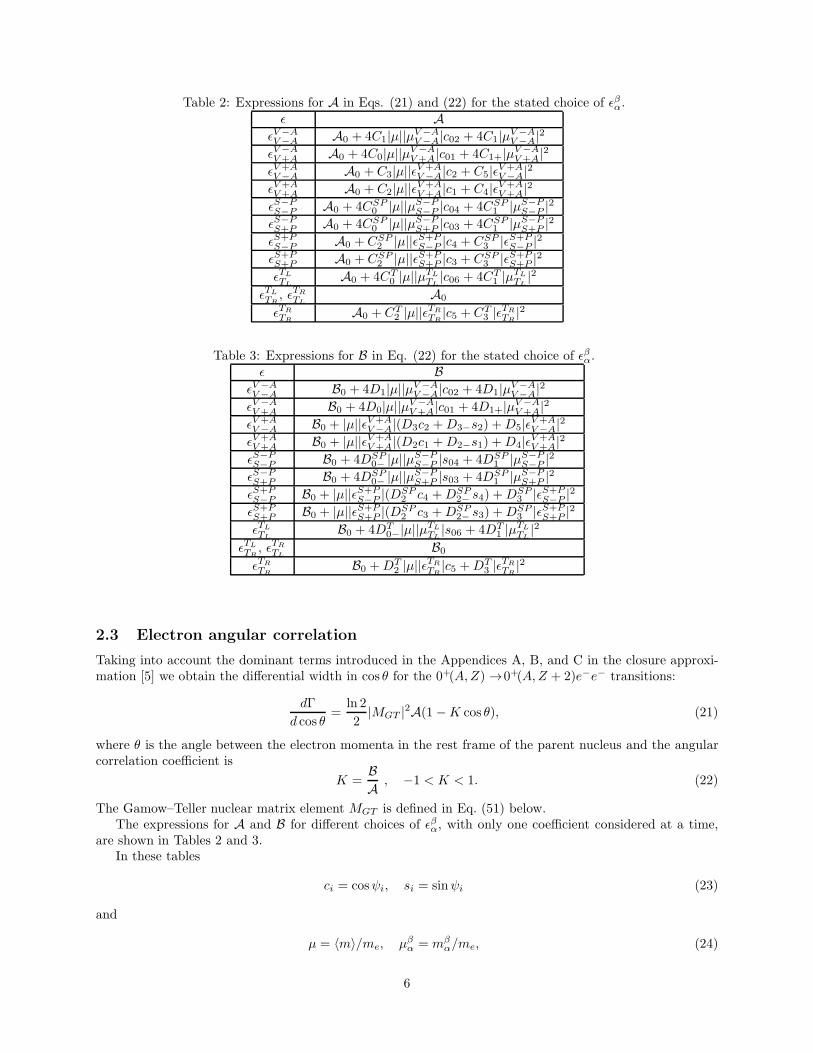
Table 2: Expressions for A in Eqs. (21) and (22) for the stated choice of ǫβα.ǫ A
ǫV−AV−A A0 + 4C1|µ||µV−A
V−A|c02 + 4C1|µV −AV −A|2
ǫV−AV+A A0 + 4C0|µ||µV −A
V +A|c01 + 4C1+|µV−AV+A|2
ǫV+AV−A A0 + C3|µ||ǫV +A
V −A|c2 + C5|ǫV+AV−A|2
ǫV+AV+A A0 + C2|µ||ǫV +A
V +A|c1 + C4|ǫV+AV+A|2
ǫS−PS−P A0 + 4CSP
0 |µ||µS−PS−P |c04 + 4CSP
1 |µS−PS−P |2
ǫS−PS+P A0 + 4CSP
0 |µ||µS−PS+P |c03 + 4CSP
1 |µS−PS+P |2
ǫS+PS−P A0 + CSP
2 |µ||ǫS+PS−P |c4 + CSP
3 |ǫS+PS−P |2
ǫS+PS+P A0 + CSP
2 |µ||ǫS+PS+P |c3 + CSP
3 |ǫS+PS+P |2
ǫTL
TLA0 + 4CT
0 |µ||µTL
TL|c06 + 4CT
1 |µTL
TL|2
ǫTL
TR, ǫTR
TLA0
ǫTR
TRA0 + CT
2 |µ||ǫTR
TR|c5 + CT
3 |ǫTR
TR|2
Table 3: Expressions for B in Eq. (22) for the stated choice of ǫβα.ǫ B
ǫV −AV −A B0 + 4D1|µ||µV−A
V−A|c02 + 4D1|µV−AV−A|2
ǫV −AV +A B0 + 4D0|µ||µV −A
V +A|c01 + 4D1+|µV −AV +A|2
ǫV +AV −A B0 + |µ||ǫV+A
V−A|(D3c2 +D3−s2) +D5|ǫV+AV−A|2
ǫV+AV+A B0 + |µ||ǫV +A
V +A|(D2c1 +D2−s1) +D4|ǫV+AV+A|2
ǫS−PS−P B0 + 4DSP
0− |µ||µS−PS−P |s04 + 4DSP
1 |µS−PS−P |2
ǫS−PS+P B0 + 4DSP
0− |µ||µS−PS+P |s03 + 4DSP
1 |µS−PS+P |2
ǫS+PS−P B0 + |µ||ǫS+P
S−P |(DSP2 c4 +DSP
2− s4) +DSP3 |ǫS+P
S−P |2ǫS+PS+P B0 + |µ||ǫS+P
S+P |(DSP2 c3 +DSP
2− s3) +DSP3 |ǫS+P
S+P |2ǫTL
TLB0 + 4DT
0−|µ||µTL
TL|s06 + 4DT
1 |µTL
TL|2
ǫTL
TR, ǫTR
TLB0
ǫTR
TRB0 +DT
2 |µ||ǫTR
TR|c5 +DT
3 |ǫTR
TR|2
2.3 Electron angular correlation
Taking into account the dominant terms introduced in the Appendices A, B, and C in the closure approxi-mation [5] we obtain the differential width in cos θ for the 0+(A,Z) →0+(A,Z + 2)e−e− transitions:
dΓ
d cos θ=
ln 2
2|MGT |2A(1 −K cos θ), (21)
where θ is the angle between the electron momenta in the rest frame of the parent nucleus and the angularcorrelation coefficient is
K =BA , −1 < K < 1. (22)
The Gamow–Teller nuclear matrix element MGT is defined in Eq. (51) below.The expressions for A and B for different choices of ǫβα, with only one coefficient considered at a time,
are shown in Tables 2 and 3.In these tables
ci = cosψi, si = sinψi (23)
and
µ = 〈m〉/me, µβα = mβ
α/me, (24)
6
with the standard effective Majorana mass 〈m〉 =∑i U2eimi and the nonstandard ones:
mS−PS∓P =
∑
i
UeiǫS−PS∓P,imi, mV −A
V ∓A =∑
i
UeiǫV−AV∓A,imi, mTL
TL,R=∑
i
UeiǫTL
TL,R,imi. (25)
The quantities A and B for all zero ǫβα are
A0 = C1|µ|2, B0 = D1|µ|2 (26)
and the relative phases are
ψ01 = arg(〈µ〉µV −A∗V +A ), ψ02 = arg(〈µ〉µV −A∗
V −A ),
ψ1 = arg(〈µ〉ǫV +A∗V +A ), ψ2 = arg(〈µ〉ǫV +A∗
V −A ),
ψ03 = arg(〈µ〉µS−P∗S+P ), ψ04 = arg(〈µ〉µS−P∗
S−P ),
ψ3 = arg(〈µ〉ǫS+P∗S+P ), ψ4 = arg(〈µ〉ǫS+P∗
S−P ),
ψ06 = arg(〈µ〉µTL∗TL
),
ψ5 = arg(〈µ〉ǫTR∗TR
), ψ6 = arg(〈µ〉ǫTR∗TL
). (27)
The coefficients Ci and C(SP,T )i in Table 2 are
C0 = (χ2F − 1)A01,
C1 = (χF − 1)2A01,
C1+ = (χF + 1)2A01,
C2 = (χF − 1)(χ2−A03 − χ1+A04),
C3 = −(χF − 1)(χ2+A03 − χ1−A04 − χ′PA05 + χ′
RA06),
C4 = χ22−A02 −
2
9χ1+χ2−A03 +
1
9χ21+A04,
C5 = χ22+A02 −
2
9χ1−χ2+A03 +
1
9χ21−A04 + χ′2
PA08 − χ′Pχ
′RA07 + χ′2
RA09; (28)
CSP0 = −(χF − 1)χSP
F ASP00 ,
CSP1 = χSP2
F ASP01 ,
CSP2 = (χF − 1)(2χSP
F0 − χSPP0 )A
SP02 ,
CSP3 = (2χSP
F0 − χSPP0 )
2ASP03 ; (29)
CT0 =
T(3)1
gA(χF − 1)AT
00,
CT1 =
(
T(3)1
gA
)2
AT01,
CT2 = −(χF − 1)
[
(χT ′RCσ
+ χT ′R + χT ′
RTσ− χT ′
RT )A01 +
(
1
3χT ′GT − 2χT ′
T
)
AT02
]
,
CT3 = (χT ′
RCσ+ χT ′
R + χT ′RTσ
− χT ′RT )
2A09 +
(
1
3χT ′GT − 2χT ′
T
)2
AT03 . (30)
The coefficients Di and D(SP,T )i entering in Table 3 are:
D0 = (χ2F − 1)B01,
D1 = (χF − 1)2B01, D1+ = (χF + 1)2B01,
7
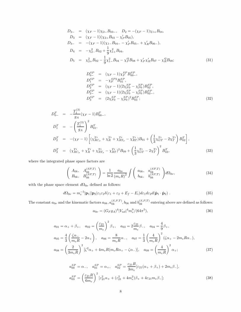
D2− = (χF − 1)χ2−B03−, D2 = −(χF − 1)χ1+B04,
D3 = (χF − 1)(χ2+B03 − χ′PB05),
D3− = −(χF − 1)(χ1−B04− − χ′PB05− + χ′
RB06−),
D4 = −χ22−B02 +
1
9χ21+B04,
D5 = χ22+B02 −
1
9χ21−B04 − χ′2
PB08 + χ′Pχ
′RB07 − χ′2
RB09; (31)
DSP0− = (χF − 1)χSP
F BSP00−,
DSP1 = −χSP2
F BSP01 ,
DSP2 = (χF − 1)(2χSP
F0 − χSPP0 )B
SP02 ,
DSP2− = (χF − 1)(2χSP
F0 − χSPP0 )B
SP02−,
DSP3 = (2χSP
F0 − χSPP0 )
2BSP03 ; (32)
DT0− = −T
(3)1
gA(χF − 1)BT
00−,
DT1 = −
(
T(3)1
gA
)2
BT01,
DT2 = −(χF − 1)
[
(χT ′RCσ
+ χT ′R + χT ′
RTσ− χT ′
RT )B01 +
(
1
3χT ′GT − 2χT ′
T
)
BT02
]
,
DT3 = (χT ′
RCσ+ χT ′
R + χT ′RTσ
− χT ′RT )
2B09 +
(
1
3χT ′GT − 2χT ′
T
)2
BT03, (33)
where the integrated phase space factors are
(
A0k, A(SP,T )0k
B0k, B(SP,T )0k
)
=1
ln 2
a0ν
(meR)2
∫
(
a0k, a(SP,T )0k
b0k, b(SP,T )0k
)
dΩ0ν , (34)
with the phase space element dΩ0ν defined as follows:
dΩ0ν = m−5e |p1||p2|ε1ε2δ(ε1 + ε2 + Ef − Ei)dε1dε2d(p1 · p2) . (35)
The constant a0ν and the kinematic factors a0k, a(S,P,T )0k , b0k and b
(S,P,T )0k entering above are defined as follows:
a0ν = (GF gA)4|Vud|4m9
e/(64π5), (36)
a01 = α+ + β+, a02 =
(
ε21me
)2
β+, a03 = 2ε21me
β−, a04 =4
9β+,
a05 =4
3
(
ζα−
meR− 2α+
)
, a06 =8
meRα−, a07 =
1
3
(
4
meR
)2
(ζα+ − 2meRα−),
a08 =
(
2
3meR
)2
[ζ2α+ + 4meR(meRα+ − ζα−)], a09 =
(
4
meR
)2
α+; (37)
aSP00 = α−, aSP
01 = α+, aSP02 =
ε21R
3me[ε21(α+ + β+) + 2meβ−],
aSP03 =
(
ε21R
6me
)2
[ε221α+ + (ε221 + 4m2e)β+ + 4ε21meβ−]; (38)
8
aT00 = 2β−, aT01 = 16α+ = 16aSP01 , aT02 =
8ζβ+meR
,
aT03 =
(
8ζ
meR
)2
β+; (39)
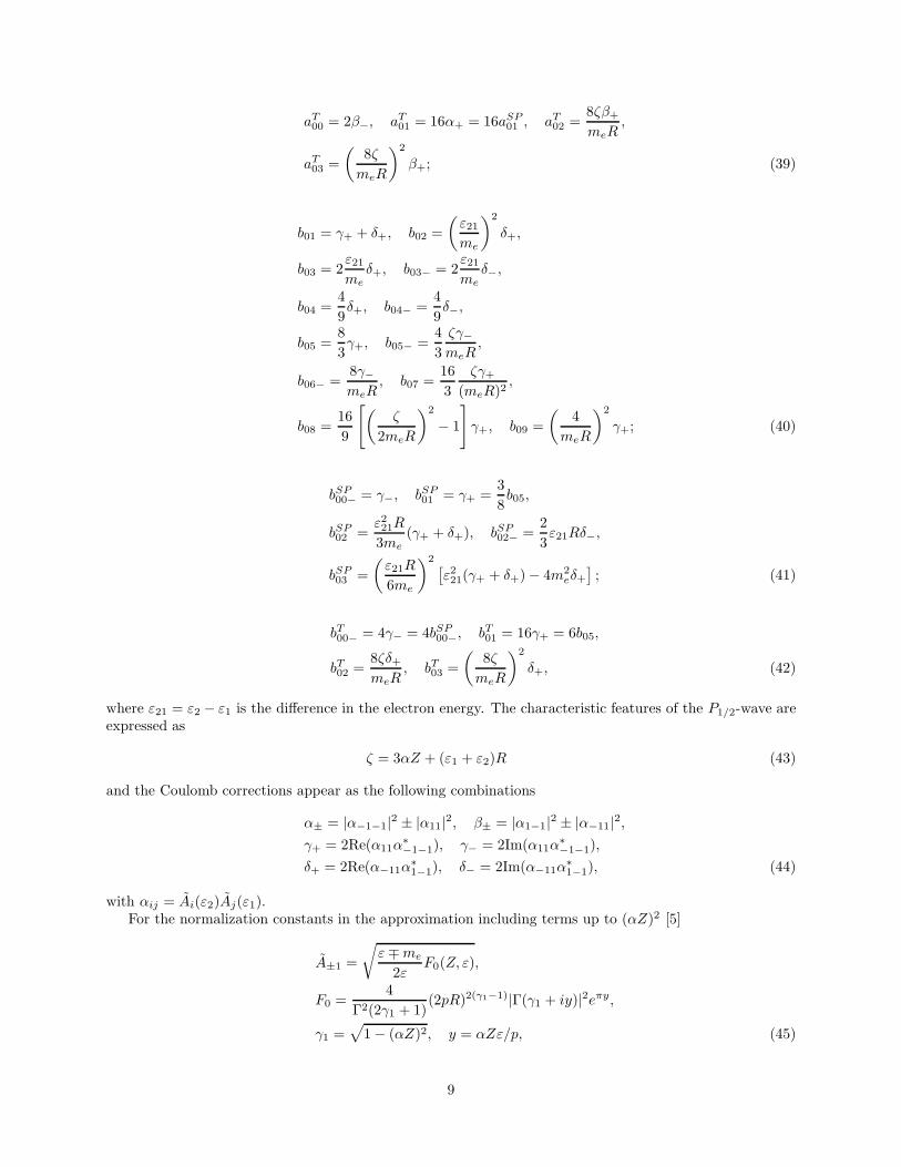
b01 = γ+ + δ+, b02 =
(
ε21me
)2
δ+,
b03 = 2ε21me
δ+, b03− = 2ε21me
δ−,
b04 =4
9δ+, b04− =
4
9δ−,
b05 =8
3γ+, b05− =
4
3
ζγ−meR
,
b06− =8γ−meR
, b07 =16
3
ζγ+(meR)2
,
b08 =16
9
[
(
ζ
2meR
)2
− 1
]
γ+, b09 =
(
4
meR
)2
γ+; (40)
bSP00− = γ−, bSP
01 = γ+ =3
8b05,
bSP02 =
ε221R
3me(γ+ + δ+), bSP
02− =2
3ε21Rδ−,
bSP03 =
(
ε21R
6me
)2[
ε221(γ+ + δ+)− 4m2eδ+]
; (41)
bT00− = 4γ− = 4bSP00−, bT01 = 16γ+ = 6b05,
bT02 =8ζδ+meR
, bT03 =
(
8ζ
meR
)2
δ+, (42)
where ε21 = ε2 − ε1 is the difference in the electron energy. The characteristic features of the P1/2-wave areexpressed as
ζ = 3αZ + (ε1 + ε2)R (43)
and the Coulomb corrections appear as the following combinations
α± = |α−1−1|2 ± |α11|2, β± = |α1−1|2 ± |α−11|2,γ+ = 2Re(α11α
∗−1−1), γ− = 2Im(α11α
∗−1−1),
δ+ = 2Re(α−11α∗1−1), δ− = 2Im(α−11α
∗1−1), (44)
with αij = Ai(ε2)Aj(ε1).For the normalization constants in the approximation including terms up to (αZ)2 [5]
A±1 =
√
ε∓me
2εF0(Z, ε),
F0 =4
Γ2(2γ1 + 1)(2pR)2(γ1−1)|Γ(γ1 + iy)|2eπy,
γ1 =√
1− (αZ)2, y = αZε/p, (45)
9
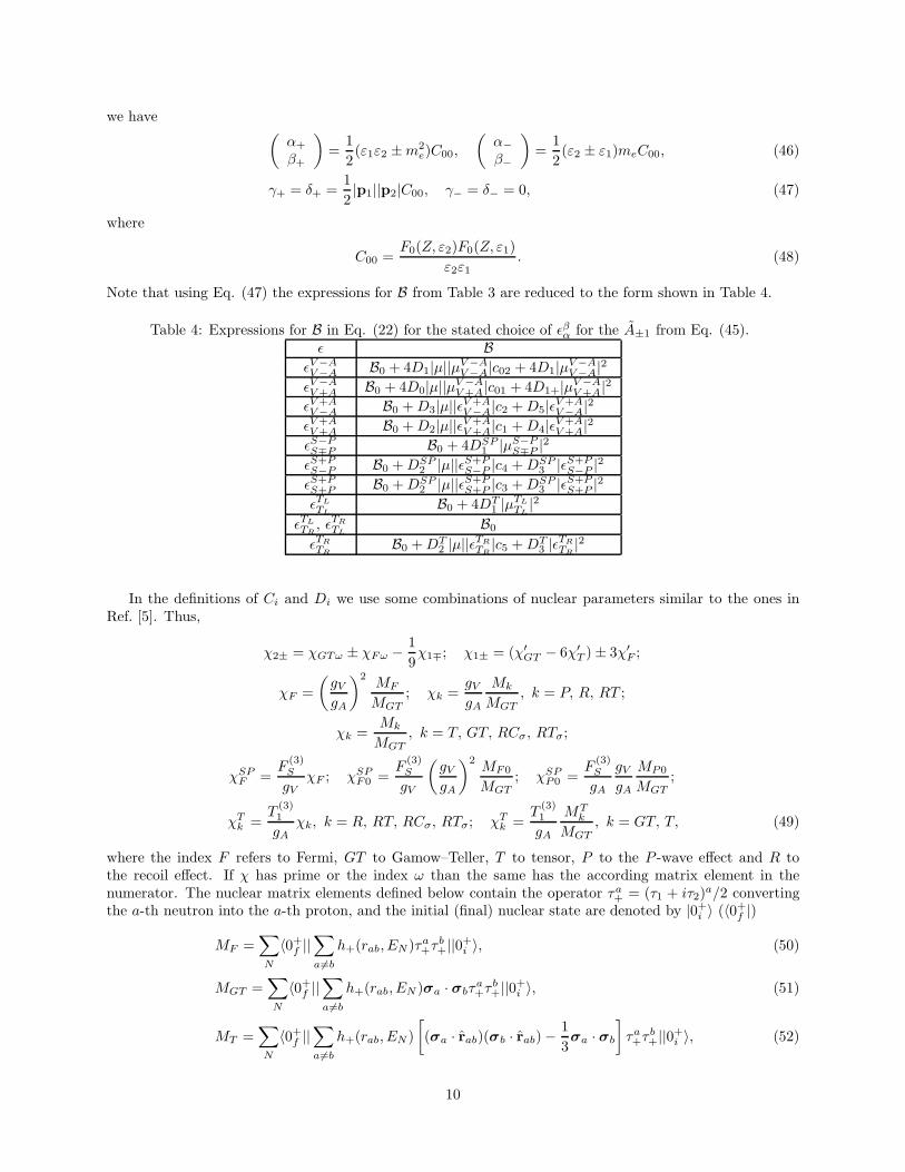
we have(
α+
β+
)
=1
2(ε1ε2 ±m2
e)C00,
(
α−
β−
)
=1
2(ε2 ± ε1)meC00, (46)
γ+ = δ+ =1
2|p1||p2|C00, γ− = δ− = 0, (47)
where
C00 =F0(Z, ε2)F0(Z, ε1)
ε2ε1. (48)
Note that using Eq. (47) the expressions for B from Table 3 are reduced to the form shown in Table 4.
Table 4: Expressions for B in Eq. (22) for the stated choice of ǫβα for the A±1 from Eq. (45).ǫ B
ǫV−AV−A B0 + 4D1|µ||µV−A
V−A|c02 + 4D1|µV−AV−A|2
ǫV−AV+A B0 + 4D0|µ||µV −A
V +A|c01 + 4D1+|µV −AV +A|2
ǫV+AV−A B0 +D3|µ||ǫV+A
V−A|c2 +D5|ǫV+AV−A|2
ǫV+AV+A B0 +D2|µ||ǫV +A
V +A|c1 +D4|ǫV+AV+A|2
ǫS−PS∓P B0 + 4DSP
1 |µS−PS∓P |2
ǫS+PS−P B0 +DSP
2 |µ||ǫS+PS−P |c4 +DSP
3 |ǫS+PS−P |2
ǫS+PS+P B0 +DSP
2 |µ||ǫS+PS+P |c3 +DSP
3 |ǫS+PS+P |2
ǫTL
TLB0 + 4DT
1 |µTL
TL|2
ǫTL
TR, ǫTR
TLB0
ǫTR
TRB0 +DT
2 |µ||ǫTR
TR|c5 +DT
3 |ǫTR
TR|2
In the definitions of Ci and Di we use some combinations of nuclear parameters similar to the ones inRef. [5]. Thus,
χ2± = χGTω ± χFω − 1
9χ1∓; χ1± = (χ′
GT − 6χ′T )± 3χ′
F ;
χF =
(
gVgA
)2MF
MGT; χk =
gVgA
Mk
MGT, k = P, R, RT ;
χk =Mk
MGT, k = T, GT, RCσ, RTσ;
χSPF =
F(3)S
gVχF ; χSP
F0 =F
(3)S
gV
(
gVgA
)2MF0
MGT; χSP
P0 =F
(3)S
gA
gVgA
MP0
MGT;
χTk =
T(3)1
gAχk, k = R, RT, RCσ, RTσ; χT
k =T
(3)1
gA
MTk
MGT, k = GT, T, (49)
where the index F refers to Fermi, GT to Gamow–Teller, T to tensor, P to the P -wave effect and R tothe recoil effect. If χ has prime or the index ω than the same has the according matrix element in thenumerator. The nuclear matrix elements defined below contain the operator τa+ = (τ1 + iτ2)
a/2 convertingthe a-th neutron into the a-th proton, and the initial (final) nuclear state are denoted by |0+i 〉 (〈0+f |)
MF =∑
N
〈0+f ||∑
a 6=b
h+(rab, EN )τa+τb+||0+i 〉, (50)
MGT =∑
N
〈0+f ||∑
a 6=b
h+(rab, EN )σa · σbτa+τ
b+||0+i 〉, (51)
MT =∑
N
〈0+f ||∑
a 6=b
h+(rab, EN )
[
(σa · rab)(σb · rab)−1
3σa · σb
]
τa+τb+||0+i 〉, (52)
10
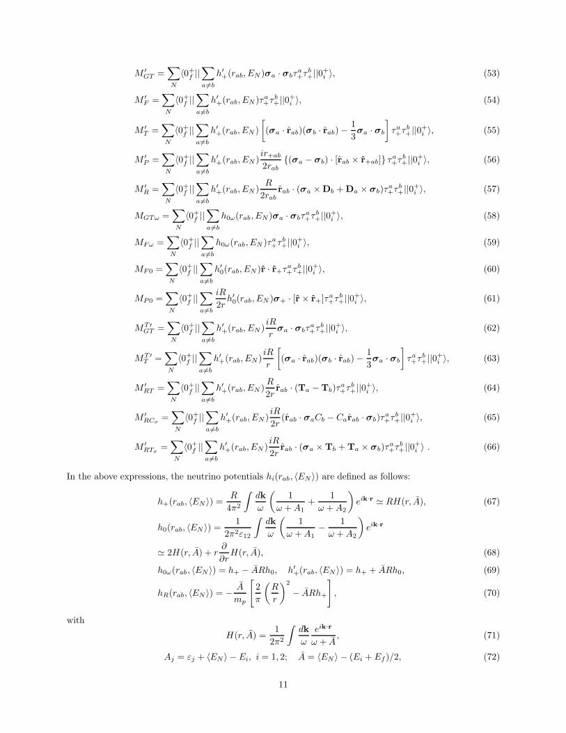
M ′GT =
∑
N
〈0+f ||∑
a 6=b
h′+(rab, EN )σa · σbτa+τ
b+||0+i 〉, (53)
M ′F =
∑
N
〈0+f ||∑
a 6=b
h′+(rab, EN )τa+τb+||0+i 〉, (54)
M ′T =
∑
N
〈0+f ||∑
a 6=b
h′+(rab, EN )
[
(σa · rab)(σb · rab)−1
3σa · σb
]
τa+τb+||0+i 〉, (55)
M ′P =
∑
N
〈0+f ||∑
a 6=b
h′+(rab, EN )ir+ab
2rab(σa − σb) · [rab × r+ab] τa+τb+||0+i 〉, (56)
M ′R =
∑
N
〈0+f ||∑
a 6=b
h′+(rab, EN )R
2rabrab · (σa ×Db +Da × σb)τ
a+τ
b+||0+i 〉, (57)
MGTω =∑
N
〈0+f ||∑
a 6=b
h0ω(rab, EN )σa · σbτa+τ
b+||0+i 〉, (58)
MFω =∑
N
〈0+f ||∑
a 6=b
h0ω(rab, EN )τa+τb+||0+i 〉, (59)
MF0 =∑
N
〈0+f ||∑
a 6=b
h′0(rab, EN )r · r+τa+τb+||0+i 〉, (60)
MP0 =∑
N
〈0+f ||∑
a 6=b
iR
2rh′0(rab, EN )σ+ · [r× r+]τ
a+τ
b+||0+i 〉, (61)
MT ′GT =
∑
N
〈0+f ||∑
a 6=b
h′+(rab, EN )iR
rσa · σbτ
a+τ
b+||0+i 〉, (62)
MT ′T =
∑
N
〈0+f ||∑
a 6=b
h′+(rab, EN )iR
r
[
(σa · rab)(σb · rab)−1
3σa · σb
]
τa+τb+||0+i 〉, (63)
M ′RT =
∑
N
〈0+f ||∑
a 6=b
h′+(rab, EN )R
2rrab · (Ta −Tb)τ
a+τ
b+||0+i 〉, (64)
M ′RCσ
=∑
N
〈0+f ||∑
a 6=b
h′+(rab, EN )iR
2r(rab · σaCb − Carab · σb)τ
a+τ
b+||0+i 〉, (65)
M ′RTσ
=∑
N
〈0+f ||∑
a 6=b
h′+(rab, EN )iR
2rrab · (σa ×Tb +Ta × σb)τ
a+τ
b+||0+i 〉 . (66)
In the above expressions, the neutrino potentials hi(rab, 〈EN 〉) are defined as follows:
h+(rab, 〈EN 〉) = R
4π2
∫
dk
ω
(
1
ω +A1+
1
ω +A2
)
eik·r ≃ RH(r, A), (67)
h0(rab, 〈EN 〉) = 1
2π2ε12
∫
dk
ω
(
1
ω +A1− 1
ω +A2
)
eik·r
≃ 2H(r, A) + r∂
∂rH(r, A), (68)
h0ω(rab, 〈EN 〉) = h+ − ARh0, h′+(rab, 〈EN 〉) = h+ + ARh0, (69)
hR(rab, 〈EN 〉) = − A
mp
[
2
π
(
R
r
)2
− ARh+
]
, (70)
with
H(r, A) =1
2π2
∫
dk
ω
eik·r
ω + A, (71)
Aj = εj + 〈EN 〉 − Ei, i = 1, 2; A = 〈EN 〉 − (Ei + Ef )/2, (72)
11
where rab is the distance between the nucleons a and b, and 〈EN 〉 is the average energy of the intermediatenucleus N .
To derive the expressions for A and B shown in Tables 2 and 3 we have used the formulas:
CA1
(
ǫS−PS∓P
)
=MGT
mS−PS∓P
me
F(3)S
gVχSPF ,
CA2
(
ǫS−PS∓P
)
= 0, CA2
(
ǫS+PS∓P
) r
r+= 2MGT ǫ
S+PS∓Pχ
SPF0 ,
CA5
(
ǫS−PS∓P
)
= 0, CA5
(
ǫS+PS∓P
) r
r+=MGT ǫ
S+PS∓Pχ
SPP0 ; (73)
ZX1
(
ǫV−AV−A
)
=MGT
(
µ+ 2µV−AV−A
)
(χF − 1),
ZX1
(
ǫV−AV+A
)
=MGT
[
µ(χF − 1) + 2µV−AV+A(χF + 1)
]
,
ZX3
(
ǫV+AV∓A
)
= ±MGT ǫV+AV∓A(χGTω ± χFω),
ZX4
(
ǫV+AV∓A
)
= ∓1
3MGT ǫ
V+AV∓Aχ1∓,
ZY6
(
ǫV+AV−A
) r
r+=MGT ǫ
V+AV−Aχ
′P ,
ZY4R
(
ǫV+AV−A
)
=MGT ǫV+AV−Aχ
′R; (74)
WU1
(
ǫTL
TL
)
= −4MGTµTL
TL
T(3)1
gA,
WV4R
(
ǫTR
TR
)
= −2MGT ǫTR
TR
T(3)1
gA(χ′
RCσ+ χ′
R + χT ′RTσ
− χT ′RT ),
WU2
(
ǫTR
TR
) r
r+= 2iMGT ǫ
TR
TR
T(3)1
gAχ′GT ,
WU7
(
ǫTR
TR
) r
r+= −4iMGT ǫ
TR
TR
T(3)1
gA
(
1
3χ′GT + 2χ′
T
)
. (75)
For all other arguments ǫβα these nucleon matrix elements have zero values, except for
ZX1
(
ǫV−AV∓A = 0
)
=MGTµ(χF − 1). (76)
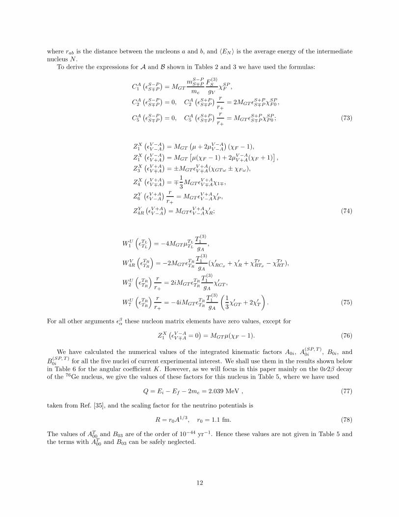
We have calculated the numerical values of the integrated kinematic factors A0i, A(SP, T )0i , B0i, and
B(SP, T )0i for all the five nuclei of current experimental interest. We shall use them in the results shown below
in Table 6 for the angular coefficient K. However, as we will focus in this paper mainly on the 0ν2β decayof the 76Ge nucleus, we give the values of these factors for this nucleus in Table 5, where we have used
Q = Ei − Ef − 2me = 2.039 MeV , (77)
taken from Ref. [35], and the scaling factor for the neutrino potentials is
R = r0A1/3, r0 = 1.1 fm. (78)
The values of AT00 and B03 are of the order of 10−44 yr−1. Hence these values are not given in Table 5 and
the terms with AT00 and B03 can be safely neglected.
12
Table 5: The integrated kinematic A- and B-factors [in 10−15yr−1] for the 0+ → 0+ transitionof the 0ν2β decay of 76Ge.
A01 6.69 B01 5.45A02 1.09×10 B02 8.95A03 3.76 B03 —A04 1.30 B04 1.21A05 2.08×10² B05 7.27A06 1.69×10³ — —A07 1.05×10⁵ B07 7.72×10⁴
A08 6.59×10³ B08 4.97×10³
A09 4.14×10⁵ B09 3.00×10⁵
ASP00 2.55 — —
ASP01 3.77 BSP
01 2.73ASP
02 1.18×10⁻¹ BSP02 7.20×10⁻²
ASP03 1.27×10⁻³ BSP
03 3.71×10⁻⁴
AT01 6.03×10 BT
01 4.36×10AT
02 1.50×10³ BT02 1.40×10³
AT03 7.67×10⁵ BT
03 7.16×10⁵
We recall that the analytic expressions associated with the coefficients ǫV+AV∓A given in this section and
the values of A0i from Table 5 confirm the results of Ref. [5]. The analytic expressions associated with the
coefficients ǫV−AV∓A, ǫ
S∓PS∓P , ǫ
TL,R
TL,Rand the values of A
(SP,T )0i , B0i, B
(SP,T )0i from Table 5 transcend the earlier
work.
3 Analysis of the electron angular correlation
3.1 Qualitative analysis
If the effects of all the interactions beyond the SM extended by the νM s, which we call the “nonstandard”effects, are zero (i.e., all ǫβα = 0), then K = B01/A01. Its values are given in Table 6 for various decayingnuclei. We will concentrate on the case of 76Ge nucleus in the following. In this case the correlation (21) isproportional to 1 − 0.81 cos θ. (Note that in the limit of me/(Ei − Ef ) → 0 we have α+ + β+ = γ+ + δ+and K = 1.) Tables 2 and 4 show that the presence of the “nonstandard” parameters ǫV−A
V∓A, ǫTL
TRor ǫTR
TL
does not change the value of K and therefore the form of the angular correlation. The presence of any otherparameter ǫβα does change this correlation. From the fact that there are no contributions due to P -wave andrecoil effects to the scalar nonstandard terms in the closure approximation (see Appendix A), it follows thatthe values of ASP
02 , ASP03 , BSP
02 , and BSP03 are small and there are two additional “nonstandard” parameters
that do not change significantly the form of the angular correlation, namely, ǫS+PS∓P .
Table 6: The values of angular correlation coefficient K for various decaying nuclei for the SM extended bythe νMs.
76Ge 82Se 100Mo 130Te 136XeK 0.81 0.88 0.88 0.85 0.84
Using Table 1 and taking into account the fact that |µβα| are suppressed in comparison with |ǫβα| by the
factor mi/me (the chiral suppression), we find the coefficient K and the set ǫ of nonzero ǫβαs that changethe 1 − 0.81 cosθ form of the correlation for the SM plus νM s, see Table 7 (the lower two entries). Theycorrespond to the following extensions of the SM: νM s plus RPV SUSY [10], νM s plus right-handed currents(RC) (connected with right-handed W bosons [5] or LQs [13]). Hence, the angular coefficient K can signalthe presence of these NP interactions.
13
Table 7: The angular correlation coefficient K for various SM extensions for decays of 76Ge.
SM extension ǫ KνM — 0.81
νM+RPV SUSY ǫTR
TR−1 < K < 1
νM+RC ǫV+AV∓A −1 < K < 1
We remark here that in our earlier analysis [19] we had neglected the P -wave and recoil effects, which isnot a good assumption. Our current study shows that these effects give significant contribution to the termswith ǫV+A
V−A and ǫTR
TR. Hence, they have to be included in any realistic analysis of the data, as and when it
becomes available. Including them, not only the model called νM+ RC but also the model νM+ RPV canessentially change the angular coefficient K from being 0.81 in the decay of the 76Ge nucleus. Left-rightsymmetric models belong to the class νM+ RC and we have studied these models in detail in section 4, wherethe correlations among the parameters K, T1/2 and either mWR or ζ are worked out for the case |〈m〉| 6= 0,cosψi = 0 considered in section 3.2.
Note that the decay half-life and angular correlation do not give any bounds on the parameters ǫTL
TRand
ǫTR
TLbecause the according expressions for A and B do not depend on them.
3.2 Quantitative analysis
Let us now consider some particular cases for the parameter space. We will analyze only the terms withǫV∓AV∓A as the corresponding nuclear matrix elements have been workd out in the literature. We use varioustypes of QRPA model for the 76Ge nucleus [20, 21] as a test case.
Using the case of |〈m〉| = 0, which gives conservative upper bounds on |µβα| and |ǫβα|, the decay half-life
is expressed from Eq. (21) as
T1/2 = ln 2/Γ =(
|MGT |2A)−1
. (79)
From Eq. (79), using Tables 2, 5 and the values of the nuclear matrix elements reported in Refs. [20, 21],we have the following expressions for the half-life [in yr] for various choices of the parameters |µV −A
V ∓A| and|ǫV+AV∓A|, taking only one parameter at a time:
T1/2 = 1.1(1.3)× 1012|µV−AV−A|−2, T1/2 = 3.2(4.0)× 1012|µV−A
V+A|−2, (80)
T1/2 = 4.0(21)× 1012|µV −AV −A|−2, T1/2 = 4.5(6.8)× 1012|µV −A
V +A|−2, (81)
T1/2 = 3.7(27)× 108|ǫV +AV −A|−2, T1/2 = 1.0(9.7)× 1013|ǫV+A
V+A|−2. (82)
Eq. (80) corresponds to using the pnQRPA model with particle-particle strength parameter gpp=1.02(1.06)[21] and Eqs (81)–(82) correspond to using the QRPA model without (with) the p-n pairing [20] (note thatthe definitions of the nuclear matrix elements χ′
P and χR in Ref. [20] differ from χ′P and χ′
R in Ref. [5] bythe factors 1/2 and 4/(meR), respectively). Comparing the numerical results in these equations, we notethat the dispersion in the half-lifes is less marked for the coefficient |µV −A
V +A|. However, the half-lifes involvingthe coefficients |µV −A
V −A| and |ǫV±AV+A| show a very strong nuclear matrix element dependence. For the QRPA
model worked out in [20], it is not clear to us if this is due to a numerical artifact or the treatment of theisoscalar neutron-proton pairing. An important, and related point, is how to fix correctly the particle-particlestrength of the nuclear Hamiltonian. Fixing the particle-particle pairing parameter, and varying it as donein [21], leads to rather stable values for the half-life of 76Ge nucleus. Clearly, these issues remain to befurther discussed and clarified. A detailed discussion of these nuclear models will take us far afield from themain point of our paper. The theoretical uncertainty in the nuclear matrix elements [2, 36] plays an essentialrole in the numerical analysis. However, as we show below, the nuclear-model dependence of the angularcoefficient K is rather modest.
14
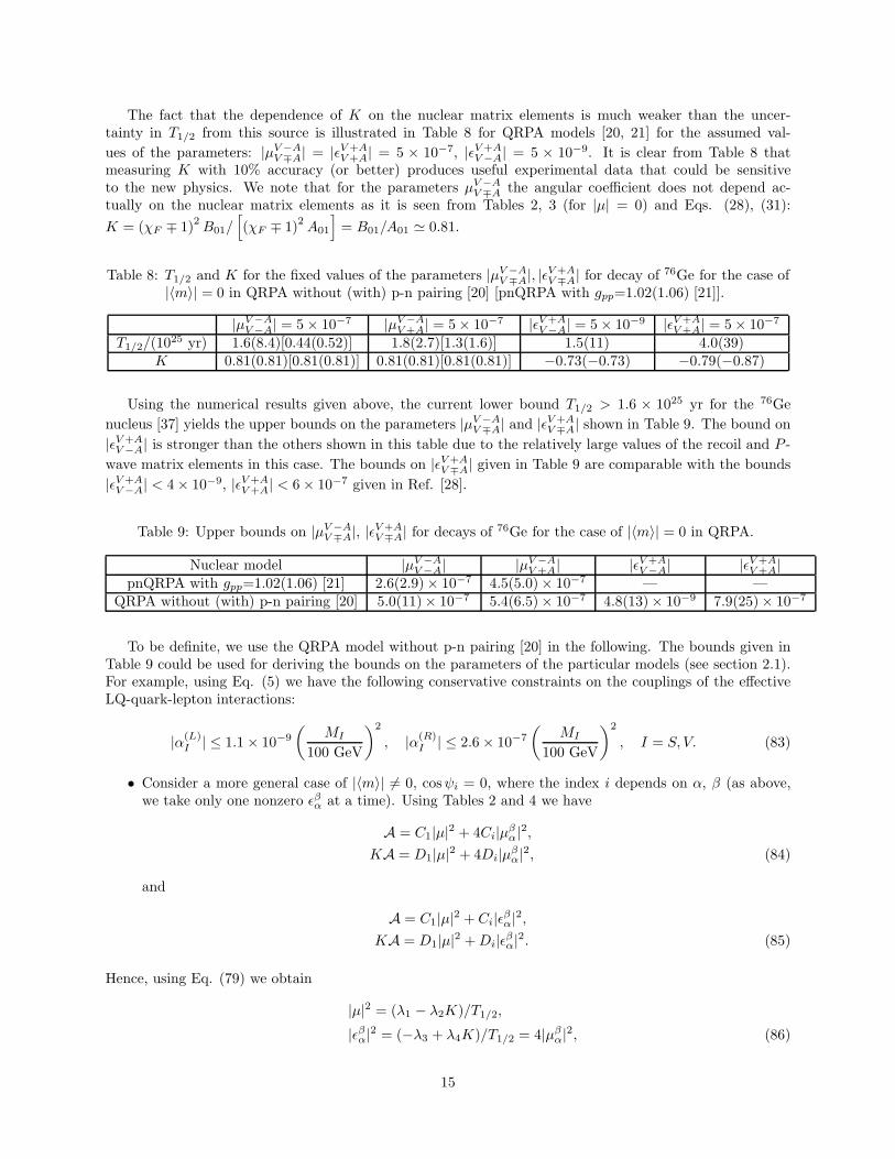
The fact that the dependence of K on the nuclear matrix elements is much weaker than the uncer-tainty in T1/2 from this source is illustrated in Table 8 for QRPA models [20, 21] for the assumed val-
ues of the parameters: |µV−AV∓A| = |ǫV+A
V+A| = 5 × 10⁻⁷, |ǫV+AV−A| = 5 × 10⁻⁹. It is clear from Table 8 that
measuring K with 10% accuracy (or better) produces useful experimental data that could be sensitiveto the new physics. We note that for the parameters µV−A
V∓A the angular coefficient does not depend ac-tually on the nuclear matrix elements as it is seen from Tables 2, 3 (for |µ| = 0) and Eqs. (28), (31):
K = (χF ∓ 1)2B01/
[
(χF ∓ 1)2A01
]
= B01/A01 ≃ 0.81.
Table 8: T1/2 and K for the fixed values of the parameters |µV −AV ∓A|, |ǫV+A
V∓A| for decay of 76Ge for the case of|〈m〉| = 0 in QRPA without (with) p-n pairing [20] [pnQRPA with gpp=1.02(1.06) [21]].
|µV −AV −A| = 5× 10⁻⁷ |µV−A
V+A| = 5× 10⁻⁷ |ǫV+AV−A| = 5× 10⁻⁹ |ǫV+A
V+A| = 5× 10⁻⁷
T1/2/(1025 yr) 1.6(8.4)[0.44(0.52)] 1.8(2.7)[1.3(1.6)] 1.5(11) 4.0(39)
K 0.81(0.81)[0.81(0.81)] 0.81(0.81)[0.81(0.81)] −0.73(−0.73) −0.79(−0.87)
Using the numerical results given above, the current lower bound T1/2 > 1.6 × 1025 yr for the 76Ge
nucleus [37] yields the upper bounds on the parameters |µV −AV ∓A| and |ǫV+A
V∓A| shown in Table 9. The bound on
|ǫV+AV−A| is stronger than the others shown in this table due to the relatively large values of the recoil and P -
wave matrix elements in this case. The bounds on |ǫV+AV∓A| given in Table 9 are comparable with the bounds
|ǫV+AV−A| < 4× 10⁻⁹, |ǫV+A
V+A| < 6× 10⁻⁷ given in Ref. [28].
Table 9: Upper bounds on |µV −AV ∓A|, |ǫV+A
V∓A| for decays of 76Ge for the case of |〈m〉| = 0 in QRPA.
Nuclear model |µV −AV −A| |µV −A
V +A| |ǫV+AV−A| |ǫV+A
V+A|pnQRPA with gpp=1.02(1.06) [21] 2.6(2.9)× 10−7 4.5(5.0)× 10−7 — —
QRPA without (with) p-n pairing [20] 5.0(11)× 10−7 5.4(6.5)× 10−7 4.8(13)× 10−9 7.9(25)× 10−7
To be definite, we use the QRPA model without p-n pairing [20] in the following. The bounds given inTable 9 could be used for deriving the bounds on the parameters of the particular models (see section 2.1).For example, using Eq. (5) we have the following conservative constraints on the couplings of the effectiveLQ-quark-lepton interactions:
|α(L)I | ≤ 1.1× 10⁻⁹
(
MI
100 GeV
)2
, |α(R)I | ≤ 2.6× 10⁻⁷
(
MI
100 GeV
)2
, I = S, V. (83)
• Consider a more general case of |〈m〉| 6= 0, cosψi = 0, where the index i depends on α, β (as above,we take only one nonzero ǫβα at a time). Using Tables 2 and 4 we have
A = C1|µ|2 + 4Ci|µβα|2,
KA = D1|µ|2 + 4Di|µβα|2, (84)
and
A = C1|µ|2 + Ci|ǫβα|2,KA = D1|µ|2 +Di|ǫβα|2. (85)
Hence, using Eq. (79) we obtain
|µ|2 = (λ1 − λ2K)/T1/2,
|ǫβα|2 = (−λ3 + λ4K)/T1/2 = 4|µβα|2, (86)
15
with the coefficients
λ1 =Di
|MGT |2∆i, λ2 =
Ci
|MGT |2∆i,
λ3 =D1
|MGT |2∆i, λ4 =
C1
|MGT |2∆i, (87)
where ∆i = C1Di −D1Ci.Using Eqs (86)–(87) we have for ǫV+A
V+A 6= 0
|µ|2 = (7.9 + 10K)× 1012/T1/2, |ǫV +AV +A|2 = (5.1− 6.3K)× 1012/T1/2 (88)
and for ǫV+AV−A 6= 0
|µ|2 = (7.7 + 10K)× 1012/T1/2, |ǫV+AV−A|2 = (1.9− 2.4K)× 108/T1/2, (89)
with T1/2 in years. Fig. 1 shows the correlation among |〈m〉|, T1/2, K (left) and the correlation among
|ǫV+AV+A|, T1/2, K (right) for the choice of a nonzero ǫV+A
V+A. Fig. 2 shows the same for the parameter ǫV+AV−A. It
is clear from Figs 1 and 2 that the closer is K to 1 for the fixed value of T1/2, the weaker is bounded |〈m〉|and stronger is bounded |ǫV+A
V∓A|. The correlations among |ǫV+AV∓A|, T1/2, K will be used in the next section in
the analysis of left-right symmetric models.Note that if several ǫβα are nonzero in the considered model than the respective interference terms should
be taken into account.
• To extract |µ|, |µβα|, |ǫβα|, ci in the general case of |〈m〉| 6= 0, ci 6= 0 we need to analyze the data on
at least two decaying nuclei. This analysis will be presented for the five nuclei already discussed in aforthcoming paper [38].
4 Electron angular correlation in left-right symmetric models
The experimental bounds on the ǫβα are connected with the masses of new particles, their mixing angles, andother parameters specific to particular extensions of the SM [5, 4, 8, 10, 12, 13]. To illustrate the kind ofcorrelations that the measurements of T1/2 and the angular correlation coefficient K in the 0ν2β decay wouldimply, we work out the case of the left-right symmetric models [22]. In the model SU(2)L × SU(2)R ×U(1)the parameters η and λ (see Eq. (2)) are expressed through the masses mWL and mWR of the left- andright-handed W bosons and their mixing angle ζ [5]:
η = − tan ζ, λ = (mWL/mWR)2, (90)
under the conditionmWL ≪ mWR . (91)
Eqs. (2) and (6) and the relation [5]Vei = V ′
ei (92)
of the SU(2)L × SU(2)R × U(1) model yield
ǫV+AV+A = λ
g′VgVUeiVei., ǫV+A
V−A = ηUeiVei. (93)
To reduce the number of free parameters, we assume the equality of the form factors of the left- and right-handed hadronic currents:
gV = g′V . (94)
The small masses of the observable νs are likely described by the seesaw formula that in the simplest casegives
mi ∼ m2D/MR, MR ≫ mD, (95)
16
with the Dirac mass scale mD (for the charged leptons and the light quarks mD ∼ 1 MeV) and the massscale MR of right νM s (in the majority of theories MR > 1 TeV). In the left-right symmetric models thesescales arise usually from the two scales of the vacuum expectation values of Higgs multiplets [22]. In theseesaw mechanism, the values of the mixing parameters Vei (for i numbering light mass states) have thesame order of magnitude as mD/MR. In our discussion we use two rather conservative values (compare withEq. (9))
ǫ = 10−6, 5× 10⁻⁷ (96)
for the mixing parameterǫ = |UeiVei|. (97)
We recall that here the summation index i runs only over the light neutrino mass eigenstates (the summationover the total mass spectrum including also heavy states gives strictly zero due to the orthogonality condition[5]).
From Eqs. (90), (93), (94), and (97) we have
mWR = mWL
(
ǫ/∣
∣ǫV+AV+A
∣
∣
)1/2, ζ = − arctan
(∣
∣ǫV+AV−A
∣
∣ /ǫ)
. (98)
Using Eq. (91) we note the approximate equality of mWL and the mass of the observed charged gauge bosonW1 (mW1
=80.4 GeV [1]).The correlation among mWR (ζ), K, and T1/2 for the case of |〈m〉| 6= 0, cosψi = 0 (see section 3.2)
is shown in Fig. 3 (4) for the two chosen values of ǫ. The numerical results for these figures have beenobtained using Eqs. (88) and (89). It is clear from Fig. 3 (4) that the closer is K to 1 for the fixed valueof T1/2 the stronger is the lower bound on mWR (the upper bound on ζ). However this bound is weakerthan the one mWR > 715 GeV, obtained from the electroweak fits [1]. There is still a more stringent boundmWR > 1.2 TeV, obtained in Ref. [39] for the 0ν2β decay mediated by heavy Majorana neutrinos usingarguments based on the vacuum stability [6] and additional theory input. We assume mWR ≥ 1 TeV in thenext figure.
While experiments in the 0ν2β decay would measure the product of the quantities called λ and theneutrino mixing matrix elements UeiVei in Eq. (93), collider experiments at the Tevatron and the LHC can,in principle, measure λ by determining mWR . Assuming these logically independent possibilities, we plotthe differential width (21) vs. cos θ in Fig. 5 for a set of values of |〈m〉| and mWR , taking ǫ
V +AV +A at a time
and assuming ǫ = 10−6. In this figure, we consider the values of |〈m〉|, starting from |〈m〉| ≤ 0.03 eV up to|〈m〉| = 5 meV, covering two of three scenarios of neutrino mass hierarchies and mixing angles: normal andinverted mass hierarchies (see Ref. [40] for a recent discussion and update). It is seen that the sensitivity ofthe electron angular correlation to the right-handed W -boson mass mWR increases with decreasing valuesof the effective Majorana neutrino mass |〈m〉|, as can be seen from Fig. 5 (right), where this correlation isshown for |〈m〉|=5 meV, 10 meV.
In conclusion, we have presented a detailed study of the electron angular correlation for the long rangemechanism of 0ν2β decays in a general theoretical context. This information, together with the ability ofobserving these decays in several nuclei, would help greatly in identifying the dominant mechanism underlyingthese decays. At present, no experiment is geared to measuring the angular correlation in 0ν2β decays, asthe main experimental thrust is on establishing a non-zero signal unambiguously in the first place. We notethat the running experiment NEMO3 has already measured the electron angular distribution for the twoneutrino double beta decay, and is capable of measuring this correlation in the future for the 0ν2β decayas well, assuming that the experimental sensitivity is sufficiently good to establish this decay [41]. Theproposed experimental facilities that can measure the electron angular correlation in the 0ν2β decays areSuperNEMO [42], MOON [43], and EXO [44]. We have argued in this paper that there is a strong case inbuilding at least one of them.
Acknowledgments
We thank Alexander Barabash and Fedor Simkovic for helpful discussions, and the referee of our paper forcritical comments which helped us in improving and correcting the earlier version of this manuscript. One
17
of us (DVZ) would like to thank DESY for the hospitality in Hamburg where a good part of this work wasdone.
A 0ν2β decay rate for scalar nonstandard terms
The nucleon currents in the impulse approximation in the nonrelativistic form are used in this paper [32, 34].Keeping all terms up to order p/mp in the nonrelativistic expansion we have
J+S∓P (x) =
∑
a
τa+δ(x− ra)(
F(3)S ∓ F
(3)P Ba
)
, Ba =σa · q2mp
, (99)
Jµ+V −A(x) =
∑
a
τa+δ(x − ra)[
gµ0(gV Ia − gACa) + gµm(gAσam − gVDma − gAP
ma )]
, (100)
Ca =σa ·Q2mp
− q0σa · qq2 +m2
π
, Dma =
Qm
2mpIa −
(
1 +gMgV
)
i[σa × q]m
2mp, Pm
a =qmσa · qq2 +m2
π
, (101)
where qµ = pµ − p′µ is the 4-momentum transferred from hadrons to leptons, Qµ = pµ + p′µ; pµ and p′µ arethe initial and final 4-momenta of a nucleon; mp is proton mass and mπ is pion mass.
We neglect the dipole dependence of the form factors F(3)S , F
(3)P , gV , gA, gM on the momentum transfer
and omit the zero argument of the form factors. Note that gV (0) = 1.Consider the pure SP case assuming 〈m〉 = 0. In terms of the combinations of hadronic currents
Jµ∓L = 〈F |J+
∓ |N〉〈N |Jµ+L |I〉, Jµ
L∓ = 〈F |Jµ+L |N〉〈N |J+
∓ |I〉, (102)
J+− = ǫS−P
S−P,iJ+S−P + ǫS−P
S+P,iJ+S+P , J+
+ = ǫS+PS+P,iJ
+S+P + ǫS+P
S−P,iJ+S−P , (103)
Jµ+L = UeiJ
µ+V−A , (104)
and the combinations
ℓL,Rµ =
sL,Rµ (2y, 1x)
ω +A1−sL,Rµ (1y, 2x)
ω +A2, (105)
ℓLλµ =sLλµ(2y, 1x)
ω +A1−sLλµ(1y, 2x)
ω +A2(106)
of electron currents
sL,Rµ (2y, 1x) = e2(y)γµ(1 ∓ γ5)e
c1(x), sLλµ(2y, 1x) = e2(y)γλ(1− γ5)γµe
c1(x), (107)
ei(x) ≡ episi(x), the matrix element is expressed as
RSP0ν =
1√2!
(
GF |Vud|√2
)2
2∑
i
∫
dxdydk
(2π)3eik·r
2ω
×∑
N
[
mi
(
Jµ−Lℓ
Rµ − Jµ
L−ℓLµ
)
+ kλ(
Jµ+Lℓ
Lλµ − Jµ
L+ℓLµλ
)]
, (108)
where r = y − x. By using the identities
sL,Rµ (1y, 2x) = sR,L
µ (2x, 1y), sLλµ(1y, 2x) = −sLµλ(2x, 1y), (109)
the algebraic formula
2(am± bn) = (a+ b)(m± n) + (a− b)(m∓ n), (110)
the constant
C0ν =G2
F |Vud|28√2π
2me
R(111)
18
and the neutrino potentials
(Hj , Hωj , Hlkj) = 4π
∫
dk
(2π)3eik·r
ω
(1, ω, kl)
ω +Aj, (112)
the matrix element (108) is expressed as
RSP0ν = −C0ν
∑
i
∑
N
(
mi
meMm
SP +MkSP
)
. (113)
Each part of this matrix element is expressed as a sum of nonvanishing (indexed by n) and vanishing(indexed by c) terms, in the closure approximation:
Mm,kSP = Mm,k
SP n + Mm,kSP c, (114)
MmSP n =
R
2
∫
dxdyTN (H1 +H2)
×[
(A1 +A1R)F05+ + (Ai
3 + Ai3R)F
i5+ +B1RF
0− + (Bi
3 + Bi3R)F
i−
]
, (115)
MmSP c =
R
2
∫
dxdyTN (H1 −H2)
×[
(A1 +A1R)F05− + (Ai
3 + Ai3R)F
i5− +B1RF
0+ + (Bi
3 + Bi3R)F
i+
]
, (116)
MkSP
n=
R
2me
∫
dxdyTN (Hω1 −Hω2)[
−(Ai4 + Ai
4R)Ei+ +B2RE−
]
+(H lk1 −H l
k2)[
−(A2 +A2R)El+ + (Alk
5 + Alk5R)E
k+ + (Bl
4 + Bl4R)E−
]
, (117)
MkSP
c=
R
2me
∫
dxdyTN (Hω1 +Hω2)[
−(Ai4 + Ai
4R)Ei− +B2RE+
]
+(H lk1 +H l
k2)[
−(A2 +A2R)El− + (Alk
5 + Alk5R)E
k− + (Bl
4 + Bl4R)E+
]
, (118)
with
TN = g2A〈F |∑
a
τa+|N〉〈N |∑
b
τb+|I〉δ(x − ra)δ(y − rb) . (119)
The electron currents are defined as:
F+ = 12 [u(yx)± u(xy)] , F5± =
1
2[u5(yx)± u5(xy)] ,
Fµ+ = 1
2 [uµ(yx)± uµ(xy)] , Fµ
5± =1
2[uµ5 (yx)± uµ5 (xy)] ,
Fµν+ = 1
2 [uµν(yx)± uµν(xy)] , Fµν
5± =1
2[uµν5 (yx)± uµν5 (xy)] ,
E± = F± + F5±, Ei± = F 0i
± + F 0i5±, (120)
with
u(yx) = e2(y)ec1(x), u5(yx) = e2(y)γ5e
c1(x),
uµ(yx) = e2(y)γµec1(x), uµ5 (yx) = e2(y)γ5γ
µec1(x),
uµν(yx) = −ie2(y)σµνec1(x), uµν5 (yx) = −ie2(y)γ5σµνec1(x) . (121)
The nucleon operator matrix elements are defined as follows:
A = A+AP , B = B +BP , (122)
19
A1 = 2G0V εS, A1R = −G0
AεSC+ −G0V εPB+,
A2 = 2G0V ε
′S, A2R = −G0
Aε′SC+ +G0
V ε′PB+,
Ai3 = G0
AεSσi+, Ai
3R = −G0AεPB
iσ+ −G0
V εSDi+, APi
3R = −G0AεSP
i+,
Ai4 = G0
Aε′Sσ
i+, Ai
4R = G0Aε
′PB
iσ+ −G0
V ε′SD
i+, APi
4R = −G0Aε
′SP
i+,
Alk5 = iεilkA
i4, Alk
5R = iεilkAi4R, (123)
B1R = −G0AεSC− +G0
V εPB−,
B2R = −G0Aε
′SC− −G0
V ε′PB−,
Bi3 = G0
AεSσi−, Bi
3R = −G0AεPB
iσ− −G0
V εSDi−, BPi
3R = −G0AεSP
i−,
Bi4 = G0
Aε′Sσ
i−, Bi
4R = G0Aε
′PB
iσ− −G0
V ε′SD
i−, BPi
4R = −G0Aε
′SP
i−, (124)
withB± = BaIb ± IaBb Bi
σ± = σiaBb ±Baσ
jb , P i
± = P iaIb ± IaP
ib . (125)
Under the exchange of running indices a and b (i.e. x ↔ y), nuclear operators A, electron currents E+
and F+ and neutrino potentials Hi and Hωi are even, while B, E−, F−, and Hki are odd.The constants are defined as:
GV =gVgA
[(
Uei + ǫV−AV−A,i
)
+ ǫV −AV +A,i
]
, GA =(
Uei + ǫV−AV−A,i
)
− ǫV −AV +A,i,
G0 = G(ǫ = 0), G0V =
gVgAUei, G0
A = Uei, (126)
εS =F
(3)S
gA
(
ǫS−PS−P,i + ǫS−P
S+P,i
)
, εP =F
(3)P
gA
(
ǫS−PS−P,i − ǫS−P
S+P,i
)
,
ε′S =F
(3)S
gA
(
ǫS+PS+P,i + ǫS+P
S−P,i
)
, ε′P =F
(3)P
gA
(
ǫS+PS+P,i − ǫS+P
S−P,i
)
. (127)
Note that in the notations of Ref. [5]:
t = u+ u5, tl = u0l + u0l5 . (128)
Since the nucleon recoil term Pa behaves as an even parity operator while the neutrino momentum k
and the recoil terms Ba, Ca, Da as odd ones, each of the Aj , k ·Aj , Bj , k ·Bj has a definite parity. Theoperators
A1, Ai3, A
i4, A
Pi3R, A
Pi4R; Bi
3, BPi3R;
r ·B4R, rlA2R, r
lAlk5R , (129)
have even parity and the operators
A1R, Ai3R, A
i4R; B1R, B2R, B
i3R;
r ·B4, r ·BP4R, r
lA2, rlAlk
5 , rlAPlk
5R , (130)
have odd parity. The odd-parity operators do not contribute to the 0+ → J+ transition in the case whereboth the electrons are in the S-wave state (the S − S case) with no de Broglie wave length correction (noFBWC).
Using the definitions of neutrino potentials
h+ =R
2(H1 +H2), h0 =
1
ε21(H1 −H2), h0ω =
R
ε21(Hω1 −Hω2),
h′+rl = −i rR
2
(
H lk1 +H l
k2
)
, h′0rl = −i r
ε21
(
H lk1 −H l
k2
)
, (131)
20
in the S − S case with no FWBC, Eqs. (115), (117) are reduced to
MmSP n,S−S =
∫
dxdyTNh+[
A1F05+ + (Ai
3 +APi3R)F
i5+
]
, (132)
MmSP c,S−S =
ε21R
2
∫
dxdyTNh0(Bi3 +BPi
3R)Fi+, (133)
MkSP
n,S−S= −1
2
ε21me
∫
dxdyTNh0ω(Ai4 +APi
4R)Ei+
+1
2
ε21me
∫
dxdyTNiR
rh′0r
l(
−A2REl+ +Alk
5REk+
)
, (134)
MkSP
c,S−S=
2
meR
∫
dxdyTNiR
2rh′+r ·B4RE+, (135)
where E, F are taken for x=0, y=0.For the 0+ → 0+ transition we have
∑
i
mi
me
∑
N
MmSP S−S = g2AC
A1 F
05+, (136)
∑
i
∑
N
MkSP
S−S= g2A
2
meRCB
4RcE+, (137)
with
CA1 = 〈mi
meh+A1〉, CB
4Rc = 〈 iR2rh′+r ·B4R〉, (138)
where r = r/r and 〈X〉 =∑i
∑
N
〈0+f ||X ||0+I 〉, with h = h(r, EN ).
In the S − P1/2 case with no FBWC for the 0+ → 0+ transition we have
MmSPn,S−P1/2
=
∫
dxdyTNh+(
Ai3RF
i5+ + Bi
3RFi−
)
, (139)
MmSP c,S−P1/2
=ε21R
2
∫
dxdyTNh0(
Ai3RF
i5− +Bi
3RFi+
)
, (140)
MkSP
n,S−P1/2= −1
2
ε21me
∫
dxdyTNh0ωAi4RE
i+
+1
2
ε21me
∫
dxdyTNiR
rh′0r
l[
−A2El+ + (Alk
5 +APlk5R )Ek
+
]
, (141)
MkSP
c,S−P1/2= − 1
meR
∫
dxdyTNh0ωAi4RE
i−
+2
meR
∫
dxdyTNiR
2rh′+r
l[
−A2El− + (Alk
5 +APlk5R )Ek
−
]
. (142)
The squared modulus of the matrix element (113), summed over the polarizations sj of the electrons andmultiplied by the phase space element (35), yields the differential decay rate for the 0+ → 0+ transition
dΓ =∑
s1,s2
|RSP0ν |2 m
5e
4π3dΩ0ν =
a0ν(meR)2
[
ASP0 − p1 · p2B
SP0
]
dΩ0ν , (143)
with a0ν being defined in Eq. (36). Here the coefficients are
ASP0 =
4∑
i=1
|Mi|2, (144)
BSP0 = Re(M1M
∗2 +M∗
1M2 +M3M∗4 +M∗
3M4), (145)
21
with
M1 = α∗−1−1
[
−CA1 +
2
meRCB
4Rc]
+
[(
meR
3
(
ζ
meR− 2
)
CA3R +
ε21R
3CA
3Rc)
r
2R
+ε221R
6me
(
CA2 − CA
5 − CA5R − CA
4R
) r
2R+
1
6
(
ζ
meR− 2
)
(
CA2 c − CA
5 c − CA5Rc − CA
4Rc)
]
+
[
(αZ)2
2meR
(
CA4 c + CA
4Rc − 3CB4RF c
)
]
, (146)
M2 = α∗11
[
CA1 +
2
meRCB
4Rc]
+
[(
meR
3
(
ζ
meR+ 2
)
CA3R − ε21R
3CA
3Rc)
r
2R
+ε221R
6me
(
CA2 − CA
5 − CA5R − CA
4R
) r
2R+
1
6
(
ζ
meR+ 2
)
(
CA2 c − CA
5 c − CA5Rc − CA
4Rc)
]
+
[
(αZ)2
2meR
(
CA4 c + CA
4Rc − 3CB4RF c
)
]
, (147)
M3 = α∗1−1
[
2
meRCB
4Rc]
+
[
ε21R
6
(
ε21me
+ 2
)
(
CA2 − CA
5 − CA5R − CA
4R
) r
2R
+1
6
ζ
meR
(
CA2 c − CA
5 c − CA5Rc − CA
4Rc)
]
+
[
(αZ)2
2meR
(
CA4 c + CA
4Rc − 3CB4RF c
)
]
, (148)
M4 = α∗−11
[
2
meRCB
4Rc]
+
[
ε21R
6
(
ε21me
− 2
)
(
CA2 − CA
5 − CA5R − CA
4R
) r
2R
+1
6
ζ
meR
(
CA2 c − CA
5 c − CA5Rc − CA
4Rc)
]
+
[
(αZ)2
2meR
(
CA4 c + CA
4Rc − 3CB4RF c
)
]
, (149)
where αij = Ai(ε2)Aj(ε1) and the nucleon matrix elements are
CB3R = 〈mi
me
i
rh+r ·B3R〉, CB
3Rc = 〈mi
me
i
2Rh0r+ ·B3R〉,
CA3R = 〈mi
me
i
2Rh+r+ ·A3R〉, CA
3Rc = 〈mi
me
i
rh0r ·A3R〉,
CA4R = 〈 i
2Rh0ωr+ ·A4R〉, CA
4Rc = 〈 iRh0ωr ·A4R〉,
CA2 = 〈 1
2rh′0r · r+A2〉, CA
2 c = 〈h′+A2〉,
CA5(R) = 〈 1
2Rh′0r
irj+Aij5(R)〉, CA
5(R)c = 〈1rh′+r
irj+Aij5(R))〉,
CB4RF = 〈 iR
2r
r2a + r2b2R2
h′+r ·B4R〉, (150)
with r+ = y + x = 2Rr+.The terms in the first brackets in Eqs. (146)–(149) come from the S − S case, the terms in the second
brackets come from the S − P1/2 case and in the third brackets there are the most important terms due tothe P1/2 − P1/2 case and FBWC.
Assuming now 〈m〉 6= 0 for the dominant terms we have
M1 = α∗−1−1
[
ZX1 − CA
1 +2
meRCB
4Rc]
+
[
ε221R
6me
(
CA2 − CA
5
) r
2R+
1
6
(
ζ
meR− 2
)
(
CA2 c − CA
5 c)
]
, (151)
22
M2 = α∗11
[
ZX1 + CA
1 +2
meRCB
4Rc]
+
[
ε221R
6me
(
CA2 − CA
5
) r
2R+
1
6
(
ζ
meR+ 2
)
(
CA2 c − CA
5 c)
]
, (152)
M3 = α∗1−1
[
ZX1 +
2
meRCB
4Rc]
+
[
ε21R
6
(
ε21me
+ 2
)
(
CA2 − CA
5
) r
2R+
1
6
ζ
meR
(
CA2 c − CA
5 c)
]
, (153)
M4 = α∗−11
[
ZX1 +
2
meRCB
4Rc]
+
[
ε21R
6
(
ε21me
− 2
)
(
CA2 − CA
5
) r
2R+
1
6
ζ
meR
(
CA2 c − CA
5 c)
]
. (154)
In the expressions for M1, ...,M4, the terms with ζ are due to the inclusion of the P -wave in the elec-tron wave function and those with CB
4R are from the inclusion of the nucleon recoil effect. In the closureapproximation there are no contributions due to the P -wave and the recoil effects. Note that some of thesubdominant terms should be taken into account in case of large cancellation among the dominant terms.
B 0ν2β decay rate for vector nonstandard terms
In this appendix we in general follow the derivation of Ref. [5]. However in addition to Ref. [5] we keep inour calculations the terms associated with the parameters ǫV−A
V∓A and the pseudoscalar form factor.The nucleon currents in the impulse approximation up to order p/mp in the nonrelativistic expansion are
[32, 34]:
Jµ+V∓A(x) =
∑
a
τa+δ(x− ra)[
gµ0(gV Ia ∓ gACa) + gµm(±gAσam − gVDma ∓ gAP
ma )]
, (155)
with Ca, Dma , Pm
a given in Eq. (101).In terms of SLµν , Vαµν , J
µναβ (α, β = L,R) [5] the matrix element
RV A0ν = C0ν
∑
i
∑
N
R
2me
∫
dxdy 4πdk
(2π)3eik·r
ω(miJ
µνLLSLµν + Jµν
LRVLµν + JµνRLVRµν) , (156)
may be expressed as
RV A0ν = C0ν
∑
i
∑
N
(
mi
meMm
VA +MkV A
)
,Mm,kV A = Mm,k
V A n + Mm,kVA c. (157)
The analogues of the Eqs. (C.2.11), (C.2.23), and (C.2.24) from Ref. [5] are as follows:
MmVAn ≡ Mmνn =
R
2
∫
dxdyTN (H1 +H2)[
(X1 + X1R)E+ + (Y i1 + Y i
1R)Ei−
]
, (158)
MmVAc ≡ Mmνc =
R
2
∫
dxdyTN (H1 −H2)[
(X1 + X1R)E− + (Y i1 + Y i
1R)Ei+
]
, (159)
MkV An ≡ MV+A(a)n =
R
me
∫
dxdyTN (Hω1 −Hω2)
×[
(X3 + X5R)F0+ + Y3RF
05− + (X l
5 + X l4R)F
l+ + (Y l
4 + Y l6R)F
l5−
]
+ (H lk1 +H l
k2)
×[
(X l5 + X l
3R)F0− + (Y l
3 + Y l5R)F
05+ + (X lk
4 + X lk6R)F
k− + (Y lk
6 + Y lk4R)F
k5+
]
, (160)
MkV Ac ≡ MV+A(a)c =
R
me
∫
dxdyTN (Hω1 +Hω2)
23
×[
(X3 + X5R)F0− + Y3RF
05+ + (X l
5 + X l4R)F
l− + (Y l
4 + Y l6R)F
l5+
]
+ (H lk1 −H l
k2)
×[
(X l5 + X l
3R)F0+ + (Y l
3 + Y l5R)F
05− + (X lk
4 + X lk6R)F
k+ + (Y lk
6 + Y lk4R)F
k5−
]
, (161)
with X = X + XP , Y = Y + Y P . The operators X and Y are defined in [5], except for the operatorY l6R = −Y l
5R which is defined to remove the minus sign from the Eqs. (160) and (161); X1 = X1S , Y1 = Y1S .The additional operators are
XP1R = G2
APiiσ+, XPl
3R = XPl4R = G−P
l+, XP
5R = GAεAPiiσ+,
XPlk6R = −GAεA
[
δlkPiiσ+ −
(
P lkσ+ + P kl
σ+
)]
+ iG+εilkPi+,
Y Pi1R = GVGAP
i− +G2
AiεijkPjkσ+, Y Plk
4R = −iG−εilkPi−,
Y Pl5R = iGAεAεlijP
ijσ+ −G+P
l−, Y Pl
6R = −iGAεAεlijPijσ+ −G+P
l−, (162)
withP ijσ+ = σi
aPjb + P i
aσjb . (163)
Under the exchange of running indices a and b, nuclear operators X , electron currents E+ and F+ andneutrino potentials Hi and Hωi are even, while Y , E−, F−, and Hki are odd.
New constants are defined as:
εV =gVgA
(
ǫV+AV+A,i + ǫV+A
V−A,i
)
, εA = ǫV+AV+A,i − ǫV+A
V−A,i. (164)
The operators
X1, XP1R; Y i
1 , YPi1R ;
X3, Xl5, X
P5R, X
Pl4R, r ·X3R, r
lX lk6R;
Y l4 , Y
Pl6R , r ·Y5R, r
lY lk4R , (165)
have even parity and the operators
X1R; Y i1R;X5R, X
l4R, r ·X5, r ·XP
3R, rlX lk
4 , rlXPlk
6R ;
Y3R, Yl6R, r ·Y3, r ·YP
5R, rlY lk
6 , rlY Plk4R , (166)
have odd parity.Using the definitions of the neutrino potentials from Eq. (131) and
hω =R2
2(Hω1 +Hω2) (167)
in the S − S case with no FBWC we have
MmVAn,S−S =
∫
dxdyTNh+(X1 +XP1R)E+, (168)
MmVAc,S−S =
ε21R
2
∫
dxdyTNh0(Yi1 + Y Pi
1R )Ei+, (169)
MkV An,S−S =
ε21me
∫
dxdyTNh0ω[
(X3 +XP5R)F
0+ + (X l
5 +XPl4R)F
l+
]
+4
meR
∫
dxdyTNiR
2rh′+r
l[
Y l5RF
05+ + Y lk
4RFk5+
]
, (170)
MkV Ac,S−S =
2
meR
∫
dxdyTNhω(Yl4 + Y Pl
6R )F l5+
+ε21me
∫
dxdyTNiR
rh′0r
l(
X l3RF
0+ +X lk
6RFk+
)
, (171)
24
where E and F are taken for x = y=0.For the 0+ → 0+ transition we have
∑
i
mi
me
∑
N
MmVAS−S = g2A(Z
X1 + ZXP
1R )E+, (172)
∑
i
∑
N
MkV A
S−S= g2A
[
ε21me
(ZX3 + ZXP
5R + ZX3Rc)F 0
+ +4
meRZY4RF
05+
]
, (173)
with
ZX1 = 〈mi
meh+X1〉, ZXP
1R = 〈mi
meh+X
P1R〉, ZX
3 = 〈h0ωX3〉,
ZY4R = 〈 iR
2rh′+r ·Y5R〉, ZXP
5R = 〈h0ωXP5R〉,
ZX3R
c= 〈 iR
rh′0r ·X3R〉. (174)
In the S − P1/2 case with no FBWC for the 0+ → 0+ transition we have
MmVAn,S−P1/2
=
∫
dxdyTNh+Yi1RE
i−, (175)
MmVAc,S−P1/2
=ε21R
2
∫
dxdyTNh0Yi1RE
i+, (176)
MkV An,S−P1/2
=ε21me
∫
dxdyTNh0ω(Xl4RF
l+ + Y l
6RFl5−)
+4
meR
∫
dxdyTNiR
2rh′+r
l[
(X lk4 +XPlk
6R )F k− + (Y lk
6 + Y Plk4R )F k
5+
]
, (177)
MkV Ac,S−P1/2
=2
meR
∫
dxdyTNhω(Xl4RF
l− + Y l
6RFl5+)
+ε21me
∫
dxdyTNiR
rh′0r
l[
(X lk4 +XPlk
6R )F k+ + (Y lk
6 + Y Plk4R )F k
5−
]
. (178)
The decay rate for the 0+ → 0+ transition takes the form
dΓ =∑
s1,s2
|R0ν |2m5
e
4π3dΩ0ν =
a0ν(meR)2
[
AV A0 − p1 · p2B
V A0
]
dΩ0ν , (179)
where the coefficients are
AV A0 =
4∑
i=1
|Ni|2, (180)
BV A0 = Re(N1N
∗2 +N∗
1N2 +N3N∗4 +N∗
3N4), (181)
with
N1 = α∗−1−1
[
ZX1 + ZXP
1R − 4
meRZY4R
]
+
[
mer
6
((
ζ
meR− 2
)
ZY1R +
ε221R
2meZY
1Rc)
+
2
3
(
ζ
meR− 2
)
(
ZY6 + ZY P
4R + ZY6Rc
) r
2R+
1
3
ε221R
me
(
ZY6R − 1
2(ZY
6 c + ZY4Rc)
)]
+
[
(αZ)2
meR(ZX
5 c + 3ZY5RF )
]
, (182)
N2 = α∗11
[
ZX1 + ZXP
1R +4
meRZY4R
]
+
[
mer
6
((
ζ
meR+ 2
)
ZY1R +
ε221R
2meZY
1Rc)
+
−2
3
(
ζ
meR+ 2
)
(
ZY6 + ZY P
4R + ZY6Rc
) r
2R− 1
3
ε221R
me
(
ZY6R − 1
2(ZY
6 c + ZY4Rc)
)]
25
+
[
− (αZ)2
meR(ZX
5 c + 3ZY5RF )
]
, (183)
N3 = α∗1−1
[
ZX1 + ZXP
1R − ε21me
(ZX3 + ZXP
5R + ZX3Rc)
]
+
[
r
6R
(
ζZY1R +
1
2ε21(ε21 + 2me)R
2ZY2R
)
+1
3
ε21me
ζ
(
ZX4R − 1
2(ZX
4 c + ZXP6R c)
)
r
2R− 1
3
(
ε21me
+ 2
)
(ZX4 + ZXP
6R − 2ZX4R)
]
, (184)
N4 = α∗−11
[
ZX1 + ZXP
1R +ε21me
(ZX3 + ZXP
5R + ZX3Rc)
]
+
[
r
6R
(
ζZY1R +
1
2ε21(ε21 − 2me)R
2ZY2R
)
−1
3
ε21me
ζ
(
ZX4R − 1
2(ZX
4 c + ZXP6R c)
)
r
2R+
1
3
(
ε21me
− 2
)
(ZX4 + ZXP
6R − 2ZX4R)
]
, (185)
where the terms in the first brackets in Eqs. (182)–(185) come from the S − S case and the terms in thesecond ones come from the S − P1/2 case. The terms in the third brackets in Eqs. (182)–(183) are the mostimportant terms of those that come from the P1/2 − P1/2 case and from the S − S case due to FBWC. Thenuclear matrix elements are
ZY1R = 〈mi
me
i
2Rh+r ·Y1R〉, ZY
1Rc = 〈mi
me
i
2Rh0r+ ·Y1R〉,
ZY6 = 〈− 1
2rh′+r
irj+Yij6 〉, ZY P
4R = 〈− 1
2rh′+r
irj+YPij4R 〉, ZY
6Rc = 〈 i
2Rhωr ·Y6R〉,
ZY6R = 〈 i
2Rh0ωr ·Y6R〉, ZY
6 c = 〈1rh′0r
irjY ij6 〉, ZY
4Rc = 〈1rh′0r
irjY ij4R〉,
ZX4R = 〈 i
2Rh0ωr+ ·X4R〉, ZX
4 c = 〈1rh′0r
irj+Xij4 〉, ZXP
6R c = 〈1rh′0r
irj+XPij6R 〉,
ZX4 = 〈1
rh′+r
irjX ij4 〉, ZX
5 c = 〈 ir2
2R2hω[ra × rb] ·X5〉, ZY
5RF = 〈 iR2r
r2a + r2b2R2
h′+r ·Y5R〉. (186)
The dominant terms give
N1 = α∗−1−1
[
ZX1 − 4
meRZY4R
]
+
[
2
3
(
ζ
meR− 2
)
ZY6
r
2R
]
, (187)
N2 = α∗11
[
ZX1 +
4
meRZY4R
]
+
[
−2
3
(
ζ
meR+ 2
)
ZY6
r
2R
]
, (188)
N3 = α∗1−1
[
ZX1 − ε21
meZX3
]
+
[
−1
3
(
ε21me
+ 2
)
ZX4
]
, (189)
N4 = α∗−11
[
ZX1 +
ε21me
ZX3
]
+
[
1
3
(
ε21me
− 2
)
ZX4
]
, (190)
that agrees with the Eq. (C.3.7) of Ref. [5] taking into account the correspondence with their notations:
ZX1 = Z1, ZX
3 = Z3, ZY6 = Z6,
ZY4R = Z4R, ZX
4R = Z5R, ZX4 = Z5, (191)
and the fact that Z2 is absent, as we have calculated only the leading contribution of the parameters ǫβα.Recall that in Ref. [5] the pseudoscalar form factor is not taken into account. However the terms associatedwith this form factor do not contribute to the dominant terms (187)–(190). Note that in the expressions forN1 and N2 given above, the terms with ζ are due to the inclusion of the P -wave in the electron wave functionand the ones with ZY
4R are due to the nucleon recoil effect. We remark that some of the subdominant terms,like those with ZX
4R, ZX4 c, ZY
6Rc, ZX5 c and ZY
5RF , should be taken into account in the case of largecancellation among the dominant terms. The same is valid for the contribution due to the pseudoscalar formfactor gAP
ia which yields corrections at about 10 % to the dominant terms.
26
C 0ν2β decay rate for tensor nonstandard terms
The nucleon currents in the impulse approximation up to order p/mp in the nonrelativistic expansion areused [32, 34], Jµ+
V −A from Eq. (100) and
Jµν+TL,R
(x) = T(3)1
∑
a
τa+δ(x− ra)
(gµkgν0 − gµ0gνk)T ka + gµmgνnεkmnσak
∓ i
2εµνρσ [(gρkgσ0 − gρ0gσk)Tak + gρrgσsεrskσak]
, (192)
T ka =
[
i(
T(3)1 − 2T
(3)2
)
qkIa + T(3)1 [σa ×Q]k
]
/(2T(3)1 mp), (193)
where, as before, qµ = pµ − p′µ is the 4-momentum transferred from hadrons to leptons, Qµ = pµ + p′µ,pµ and p′µ are the initial and final 4-momenta of a nucleon. We neglect the dipole dependence of the form
factors T(3)1 and T
(3)2 on the momentum transfer and omit the zero argument of the form factors.
Consider the pure TL,R case assuming 〈m〉 = 0. In terms of the hadronic currents
JαµνLTL,R
= 〈F |Jα+L |N〉〈N |Jµν+
TL,R|I〉, Jµνα
TL,RL = 〈F |Jµν+TL,R
|N〉〈N |Jα+L |I〉, (194)
Jµν+TL
= ǫTL
TL,iJµν+TL
+ ǫTL
TR,iJµν+TR
, Jµν+TR
= ǫTR
TR,iJµν+TR
+ ǫTR
TL,iJµν+TL
, (195)
Jµ+L = UeiJ
µ+V −A , (196)
and the leptonic tensors
ℓ1αµν =t1αµν(2y, 1x)
ω +A1−t1αµν(1y, 2x)
ω +A2, (197)
ℓ1αλµν =t1αλµν(2y, 1x)
ω +A1−t1αλµν(1y, 2x)
ω +A2, (198)
ℓ2µνα =t2µνα(2y, 1x)
ω +A1−t2µνα(1y, 2x)
ω +A2, (199)
ℓ2µνλα =t2µνλα(2y, 1x)
ω +A1−t2µνλα(1y, 2x)
ω +A2, (200)
with the electron currents defined as
t1αµν(2y, 1x) = e2(y)γα(1− γ5)σµνec1(x),
t1αλµν(2y, 1x) = e2(y)γα(1− γ5)γλσµνec1(x),
t2µνα(2y, 1x) = e2(y)σµν (1− γ5)γαec1(x),
t2µνλα(2y, 1x) = e2(y)σµνγλ(1− γ5)γαec1(x) , (201)
the matrix element is expressed as
RT0ν =
1√2!
(
GF |Vud|√2
)2
2∑
i
∫
dxdydk
(2π)3eik·r
2ω
×∑
N
[
mi
(
JαµνLTL
ℓ1αµν + JµναTLLℓ
2µνα
)
+ kλ(
JαµνLTR
ℓ1αλµν + JµναTRLℓ
2µνλα
)]
. (202)
For the electron currents we have the identities
t1αµν(1y, 2x) = −t2µνα(2y, 1x),t1αλµν (1y, 2x) = t2µνλα(2y, 1x). (203)
27
Using Eqs (110), (111), and (112), the matrix element (202) is expressed as
RT0ν = C0ν
∑
i
∑
N
(
mi
meMm
T +MkT
)
, (204)
Mm,kT = Mm,k
T n + Mm,kT c, (205)
with nonvanishing (n) and vanishing (c) in the closure approximation parts:
MmT n = R
∫
dxdyTN (H1 +H2)
×[
(U1 + U1R)F05+ + (U i
3 + U i3R)F
i5+ + V1RF
0− + (V i
3 + V i3R)F
i−
]
, (206)
MmT c = R
∫
dxdyTN (H1 −H2)
×[
(U1 + U1R)F05− + (U i
3 + U i3R)F
i5− + V1RF
0+ + (V i
3 + V i3R)F
i+
]
, (207)
MkT
n=
R
me
∫
dxdyTN (Hω1 −Hω2)[
V2RE− + (U i4 + U i
4R)F0i+ + (U ij
6 + U ij6R)F
ij+
]
+(Hik1 +Hi
k2)[
(V i4 + V i
4R)E+ + (U2 + U2R)F0i− + (U j
5 + U j5R)F
ij− + (U ij
7 + U ij7R)F
0j−
+(U ijk8 + U ijk
8R )F jk−
]
, (208)
MkT
c=
R
me
∫
dxdyTN (Hω1 +Hω2)[
V2RE+ + (U i4 + U i
4R)F0i− + (U ij
6 + U ij6R)F
ij−
]
+(Hik1 −Hi
k2)[
(V i4 + V i
4R)E− + (U2 + U2R)F0i+ + (U j
5 + U j5R)F
ij+ + (U ij
7 + U ij7R)F
0j+
+(U ijk8 + U ijk
8R )F jk+
]
, (209)
where the nucleon operators are
U = U + UP , V = V + V P , (210)
U1 = −2G0A(εT1
+ εT2)σaσb, UP
1R = G0A(εT1
+ εT2)P ii
σ+,
U1R = G0V (εT1
+ εT2)Dii
σ+ − iG0A(εT1
+ εT2)T ii
σ+,
U2 = 2iG0A(ε
′T1
+ ε′T2)σaσb, UP
2R = −iG0A(ε
′T1
+ ε′T2)P ii
σ+,
U2R = −iG0V (ε
′T1
+ ε′T2)Dii
σ+ +G0A(ε
′T1
+ ε′T2)T ii
σ+,
U i3 = −G0
V (εT1+ εT2
)σi+, UPi
3R = −iG0A(εT1
+ εT2)εijkP
jkσ−,
U i3R = G0
A(εT1+ εT2
)Ciσ+ − iG0
V (εT1+ εT2
)εijkDjkσ−
− iG0V (εT1
+ εT2)T i
+ − iG0A(εT1
+ εT2)εijkT
jkσ−,
U i4 = −iG0
V (ε′T1
+ ε′T2)σi
+, UPi4R = −G0
A(ε′T1
+ ε′T2)εijkP
jkσ−,
U i4R = iG0
A(ε′T1
+ ε′T2)Ci
σ+ −G0V (ε
′T1
+ ε′T2)εijkD
jkσ−
− G0V (ε
′T1
+ ε′T2)T i
+ + iG0A(ε
′T1
+ ε′T2)εijkT
jkσ−,
U i5 = −iG0
V (ε′T1
+ ε′T2)σi
+, UPi5R = G0
Aε′T1εijkP
jkσ−,
U i5R = −iG0
A(ε′T1
+ ε′T2)Ci
σ+ +G0V ε
′T1εijkD
jkσ−
− G0V (ε
′T1
+ ε′T2)T i
+ + iG0Aε
′T2εijkT
jkσ−,
U ij6 =
1
2G0
V (ε′T1
+ ε′T2)εijkσ
k+, UPij
6R = iG0A(ε
′T1
+ ε′T2)P ij
σ+,
28
U ij6R = −1
2G0
A(ε′T1
+ ε′T2)εijkC
kσ+ − i
2G0
V (ε′T1
+ ε′T2)εijkT
k+
+ iG0V (ε
′T1
+ ε′T2)Dij
σ+ − iG0A(ε
′T1
+ ε′T2)T ij
σ+,
U ij7 = +G0
V (ε′T1
+ ε′T2)εijkσ
k+ − 2iG0
A(ε′T1
+ ε′T2)(σi
aσjb + σj
aσib),
U ij7R = −G0
A(ε′T1
+ ε′T2)εijkC
kσ+ − iG0
V (ε′T1
+ ε′T2)εijkT
k+
+ iG0V (ε
′T1
+ ε′T2)(Dij
σ+ + Djiσ+)−G0
A(ε′T1
+ ε′T2)(T ij
σ+ + T jiσ+),
UPij7R = +iG0
A(ε′T1
+ ε′T2)(P ij
σ+ + P jiσ+),
U ijk8 = +
1
2G0
A(ε′T1
+ ε′T2)[εljk(σ
iaσ
lb + σl
aσib) + 2εilj(σ
laσ
kb + σk
aσlb)],
U ijk8R = −1
2G0
V (ε′T1
+ ε′T2)εljkD
liσ+ −G0
V εilj(ε′T1Dlk
σ+ + ε′T2Dkl
σ+)
− i
2G0
A(ε′T1
+ ε′T2)εljkT
ilσ+ − iG0
Aεilj(ε′T1T lkσ+ + ε′T2
T klσ+),
UPijk8R = −1
2G0
A(ε′T1
+ ε′T2)εljkP
liσ+ −G0
Aεilj(ε′T1P lkσ+ + ε′T2
P klσ+), (211)
V1R = −G0V (εT1 + εT2)D
iiσ− − iG0
A(εT1 + εT2)Tiiσ−, V P
1R = −G0A(εT1 + εT2
)P iiσ−,
V2R = −G0V (ε
′T1 + ε′T2)D
iiσ− + iG0
A(ε′T1 + ε′T2)T
iiσ−, V P
2R = −G0A(ε
′T1 + ε′T2
)P iiσ−,
V i3 = G0
V (εT1+ εT2
)σi− + 2iG0
A(εT1+ εT2
)[σa × σb]i,
V i3R = −G0
A(εT1 + εT2)Ciσ− + iG0
V (εT1+ εT2
)εijkDjkσ+
+ iG0V (εT1
+ εT2)T i
− − iG0A(εT1
+ εT2)εijkT
jkσ+,
V Pi3R = iG0
A(εT1+ εT2
)εijkPjkσ+,
V i4 = G0
V (ε′T1
+ ε′T2)σi
− − 2iG0A(ε
′T1
+ ε′T2)[σa × σb]
i,
V i4R = −G0
A(ε′T1 + ε′T2)C
iσ− + iG0
V (ε′T1
+ ε′T2)εijkD
jkσ+
− iG0V (ε
′T1
+ ε′T2)T i
− −G0A(ε
′T1
+ ε′T2)εijkT
jkσ+,
V Pi4R = iG0
A(ε′T1
+ ε′T2)εijkP
jkσ+, (212)
withT i± = T i
aIb ± IaTib , T ij
σ± = σiaT
jb ± T i
aσjb , X
ijσ± = σi
aXjb ±Xj
aσib, X = D, T, P. (213)
Under the exchange of indices a and b, nuclear operators U , electron currents F+ and neutrino potentialsHi and Hωi are even, while V , F−, and Hki are odd.
The new constants are defined as:
εT1=T
(3)1
gA
(
ǫTL
TL,i + ǫTL
TR,i
)
, εT2=T
(3)1
gA
(
ǫTL
TL,i − ǫTL
TR,i
)
,
ε′T1=T
(3)1
gA
(
ǫTR
TR,i + ǫTR
TL,i
)
, ε′T2=T
(3)1
gA
(
ǫTR
TR,i − ǫTR
TL,i
)
. (214)
The even parity operators are
U1, UP1R, k
iU2R, Ui3, U
Pi3R, U
i4, U
Pi4R, k
iU j5R, U
ij6 , U
Pij6R , kiU ij
7R, kiU ijk
8R ;
V P1R, V
P2R, V
i3 , V
Pi3R , k ·V4R; (215)
and the odd parity operators are
U1R, kiU2, k
iUP2R, U
i3R, U
i4R, k
iU j5 , k
iUPj5R , U
ij6R, k
iU ij7 , k
iUPij7R ,
kiU ijk8 , kiUPijk
8R ; V1R, V2R, Vi3R, k ·V4, k ·VP
4R. (216)
29
Using the definitions of the neutrino potentials from Eqs. (131) and (167), in the S − S case with noFBWC we have
MmT n,S−S = 2
∫
dxdyTNh+[
(U1 + UP1R)F
05+ + (U i
3 + UPi3R)F
i5+
]
, (217)
MmT c,S−S = ε21R
∫
dxdyTNh0[
V P1RF
0+ + (V i
3 + V Pi3R )F i
+
]
, (218)
MkT
n,S−S=ε21me
∫
dxdyTNh0ω
[
(U i4 + UPi
4R)F0i+ + (U ij
6 + UPij6R )F ij
+
]
+4
meR
∫
dxdyTNiR
2rh′+r ·V4RE+, (219)
MkT
c,S−S=
2
meR
∫
dxdyTNhωVP2RE+
+ε21me
∫
dxdyTNiR
rh′0r
i[
U2RF0i+ + U j
5RFij+ + U ij
7RF0j+ + U ijk
8R Fjk+
]
, (220)
where E and F are taken for x = y = 0.For the 0+ → 0+ transition we have
∑
i
mi
me
∑
N
MmT S−S = g2A
[
2(WU1 +WUP
1R )F 05+ + ε21RWV P
1R cF 0+
]
, (221)
∑
i
∑
N
MkT
S−S=
2g2AmeR
(2WV4R + WV P
2R c)E+, (222)
with
WU1 = 〈mi
meh+U1〉, WUP
1R = 〈mi
meh0U
P1R〉, WV P
1R c = 〈mi
meh0V
P1R〉,
WV4R = 〈 iR
2rh′+r ·V4R〉,
WV P2R
c= 〈hωV P
2R〉. (223)
In the S − P1/2 case with no FBWC for the 0+ → 0+ transition we have
MmT n,S−P1/2
= 2
∫
dxdyTNh+(
U i3RF
i5+ + V i
3RFi−
)
, (224)
MmT c,S−P1/2
= ε21R
∫
dxdyTNh0(
U i3RF
i5− + V i
3RFi+
)
, (225)
MkTn,S−P1/2
=ε21me
∫
dxdyTNh0ωUi4RF
0i+
+4
meR
∫
dxdyTNiR
2rh′+r
i[
(U2 + UP2R)F
0i− + (U ij
7 + UPij7R )F 0j
−
]
, (226)
MkTc,S−P1/2
=2
meR
∫
dxdyTNhωUi4RF
0i−
+ε21me
∫
dxdyTNiR
rh′0r
i[
(U2 + UP2R)F
0i+ + (U ij
7 + UPij7R )F 0j
+
]
. (227)
The decay rate for the 0+ → 0+ transition takes the form
dΓ =∑
s1,s2
|R0ν |2m5
e
4π3dΩ0ν =
a0ν(meR)2
[
AT0 − p1 · p2B
T0
]
dΩ0ν , (228)
where the coefficients are
AT0 =
4∑
i=1
|Oi|2, (229)
BT0 = Re(O1O
∗2 +O∗
1O2 +O3O∗4 +O∗
3O4), (230)
30
with
O1 = α∗−1−1
[
−2(WU1 +WUP
1R ) +2
meR(WV
4R + WV P2R c)
]
+
[
mer
3
(
ζ
meR− 2
)
WU3R +
ε221rR
6WU
3Rc]
+
[
−3(αZ)2
meR
(
WV4RF +
1
2WV P
2RF c)]
, (231)
O2 = α∗11
[
2(WU1 +WUP
1R ) +2
meR(WV
4R + WV P2R c)
]
+
+
[
−mer
3
(
ζ
meR+ 2
)
WU3R +
ε221rR
6WU
3Rc]
+
[
−3(αZ)2
meR
(
WV4RF +
1
2WV P
2RF c)]
, (232)
O3 = α∗1−1
[
−ε21RWV P1R c +
2
meR(WV
4R + WV P2R c)
]
+
[
mer
3
(
ε21me
+ 2
)
WV3R + ζ
ε21r
6WV
3Rc
+ε21R
3
(
ε21me
+ 2
)
(WU4R − WU
2 c − WU7 c − WUP
2R c − WUP7R c)
−4
3
ζ
meR(WU
2 +WU7 +WUP
2R +WUP7R − 1
2WU
4Rc)]
+
[
−3(αZ)2
meR
(
WV4RF +
1
2WV P
2RF c)]
,(233)
O4 = α∗−11
[
ε21RWV P1R c +
2
meR(WV
4R + WV P2R c)
]
+
[
−mer
3
(
ε21me
− 2
)
WV3R − ζ
ε21r
6WV
3Rc
+ε21R
3
(
ε21me
− 2
)
(WU4R − WU
2 c − WU7 c − WUP
2R c − WUP7R c)
−4
3
ζ
meR(WU
2 +WU7 +WUP
2R +WUP7R − 1
2WU
4Rc)]
+
[
−3(αZ)2
meR
(
WV4RF +
1
2WV P
2RF c)]
,(234)
where the terms in the first brackets in Eqs. (231)–(234) come from the S − S case and the terms in thesecond ones come from the S − P1/2 case. The terms in the third brackets in Eqs. (231)-(232) are the mostimportant terms of those that come from the S − S case due to FBWC. Note that in the S − S case thereis the contribution to Eqs. (231) and (232) from the (Hω1 +Hω2) combination in Eq. (209). Therefore thecontribution from the P1/2 − P1/2 case should not be taken into account.
The nuclear matrix elements are
WU3R = 〈mi
me
i
2Rh+r+ ·U3R〉, WU
3Rc = 〈mi
me
i
rh0r ·U3R〉,
WV3R = 〈mi
me
i
rh+r ·V3R〉, WV
3Rc = 〈mi
me
i
2Rh0r+ ·V3R〉,
WU4R = 〈 i
2Rh0ωr+ ·U4R〉,
WU2 c = 〈R
rh′0r · r+U2〉, WUP
2R c = 〈Rrh′0r · r+UP
2R〉,
WU7 c = 〈R
rh′0r
irj+Uij7 〉, WUP
7R c = 〈Rrh′0r
irj+UPij7R 〉. (235)
Assuming now 〈m〉 6= 0 for the dominant terms we have
O1 = α∗−1−1
[
ZX1 − 2WU
1 +2
meR(WV
4R + WV P2R c)
]
+
, (236)
O2 = α∗11
[
ZX1 + 2WU
1 +2
meR(WV
4R + WV P2R c)
]
+
, (237)
31
O3 = α∗1−1
[
ZX1 +
2
meR(WV
4R + WV P2R c)
]
+
[
ε21R
3
(
ε21me
+ 2
)
(WU4R − WU
2 c − WU7 c)−
4
3
ζ
meR(WU
2 +WU7 )
]
+
, (238)
O4 = α∗−11
[
ZX1 +
2
meR(WV
4R + WV P2R c)
]
+
[
ε21R
3
(
ε21me
− 2
)
(WU4R − WU
2 c − WU7 c)−
4
3
ζ
meR(WU
2 +WU7 )
]
+
. (239)
Again, in the above expressions, the terms with ζ are due to the inclusion of the P -wave in the electronwave function and the ones with WV P
2R and WX4R (X = U, V ) are due to the nucleon recoil effect.
32
References
[1] Particle Data Group: W.-M. Yao et al., J. Phys. G33, 1 (2006).
[2] S.R. Elliot and P. Vogel, Ann. Rev. Nucl. Part. Sci. 52, 115 (2002); P. Vogel, arXiv:hep-ph/0611243.
[3] Ya.B. Zeldovich and M.Yu. Khlopov, JETP Lett. 34, 141 (1981); Sov. Phys. Usp. 24, 755 (1981).
[4] M.G. Shchepkin, Sov. Phys. Usp. 27, 555 (1984).
[5] M. Doi, T. Kotani, and E. Takasugi, Prog. Theor. Phys. Suppl. 83, 1 (1985).
[6] R.N. Mohapatra, Phys. Rev. D34, 3457 (1986).
[7] J.D. Vergados, Phys. Lett. B184, 55 (1987).
[8] M. Hirsch, H.V. Klapdor-Kleingrothaus, and S.G. Kovalenko, Phys. Rev. Lett. 75, 17 (1995); Phys.Lett. B352, 1 (1995); Phys. Lett. B403, 291 (1997); Nucl. Phys. Proc. Suppl. A52, 257 (1997); Phys.Rev. D57, 1947 (1998).
[9] K.S. Babu and R.N. Mohapatra, Phys. Rev. Lett. 75, 2276 (1995).
[10] M. Hirsch, H.V. Klapdor-Kleingrothaus, and S.G. Kovalenko, Phys. Lett. B372, 181 (1996); B381, 488(Erratum) (1996); H. Pas, M. Hirsch, and H.V. Klapdor-Kleingrothaus, Phys.Lett. B459, 450 (1999).
[11] A. Faessler, S.G. Kovalenko, F. Simkovic, and J. Schwieger, Phys. Rev. Lett. 78, 183 (1997).
[12] H.V. Klapdor-Kleingrothaus and U. Sarkar, Phys. Lett. B554, 45 (2003).
[13] M. Hirsch, H.V. Klapdor-Kleingrothaus, and S.G. Kovalenko, Phys. Rev. D54, 4207 (1996).
[14] M. Hirsch, H.V. Klapdor-Kleingrothaus, and O. Panella, Phys. Lett. B374, 7 (1996).
[15] J.D. Vergados, Nucl. Phys. B (Proc. Suppl.) 143, 211 (2005) [arXiv:hep-ph/0409319].
[16] J. Schechter and J.W. Valle, Phys. Rev. D25, 2951 (1982); E. Takasugi, Phys. Lett. B149, 372 (1984);J.F. Nieves, Phys. Lett. B147, 375 (1984).
[17] F. Deppisch and H. Pas, Phys. Rev. Lett. 98, 232501 (2007) [arXiv:hep-ph/0612165].
[18] V.M. Gehman and S.R. Elliott, J. Phys. G 34, 667 (2007) [arXiv:hep-ph/0701099].
[19] A. Ali, A.V. Borisov, and D.V. Zhuridov, arXiv:hep-ph/0606072.
[20] G. Pantis, F. Simkovic, J.D. Vergados, and A. Faessler, Phys. Rev. C53, 695 (1996).
[21] M. Kortelainen and J. Suhonen, Phys. Rev. C 75, 051303 (2007) [arXiv:0705.0469 [nucl-th]].
[22] J.C. Pati and A. Salam, Phys. Rev. D10, 275 (1974); R.N. Mohapatra and J.C. Pati, Phys. Rev. D11,566, 2558 (1975); G. Senjanovic and R.N. Mohapatra, Phys. Rev. D12, 1502 (1975); R.N. Mohapatraand G. Senjanovic, Phys. Rev. D23, 165 (1981).
[23] H. Pas, M. Hirsch, H.V. Klapdor-Kleingrothaus, and S.G. Kovalenko, Phys. Lett. B453, 194 (1999).
[24] G. Gamov and E. Teller, Phys. Rev. 49, 895 (1936); S.F. Novaes, in “Particle and Fields”, Proc. 10thJ.A. Swieca Summer School, Sao Paulo, Brazil, 31 Jan – 12 Feb 1999 (World Scientific, Singapore, 2000)[arXiv:hep-ph/0001283].
[25] B. Pontecorvo, Sov. Phys. JETP 6, 429 (1958); Z. Maki, M. Nakagawa, and S. Sakata, Prog. Theor.Phys. 28, 870 (1962).
[26] J.C. Pati and A. Salam, Phys. Lett. B58, 333 (1975).
33
[27] W. Buchmuller, R. Ruckl, and D. Wyler, Phys. Lett. B191, 442 (1987).
[28] H.V. Klapdor-Kleingrothaus and H. Pas, in COSMO 99: 3rd International Conference on ParticlePhysics and the Early Universe, Trieste, Italy, 27 Sep – 3 Oct 1999; in H.V. Klapdor-Kleingrothaus (Ed.),“Sixty Years of Double Beta Decay” (World Scientific, Singapore, 2001), p. 755 [arXiv:hep-ph/0002109].
[29] N. Severijns, M. Beck, and O. Naviliat-Cuncic, Rev. Mod. Phys. 78, 991 (2006) [arXiv:nucl-ex/0605029].
[30] M.E. Rose, Relativistic Electron Theory (Wiley, New York, 1961).
[31] S.L. Adler et al., Phys. Rev. D11, 3309 (1975).
[32] T. Tomoda, Rep. Prog. Phys. 54, 53 (1991).
[33] J.D. Vergados, Phys. Rep. 361, 1 (2002).
[34] T. Ericson and W. Weise, Pions and Nuclei (Clarendon Press, Oxford, 1988).
[35] K. Zuber, Preprint IPPP-05-56, DCPT-05-114 ( 2005). Presented at IPPP Workshop on Matrix Ele-ments for Neutrinoless Double Beta Decay, Durham, England, 23–24 May 2005 [arXiv:nucl-ex/0511009].
[36] V.A. Rodin, A. Faessler, F. Simkovic, and P. Vogel, Czech. J. Phys. 56, 495 (2006); arXiv:0706.4304[nucl-th].
[37] C.E. Aalseth et al., Phys. Rev. D70, 078302 (2004).
[38] A. Ali, A.V. Borisov, and D.V. Zhuridov (work in progress).
[39] H.V. Klapdor-Kleingrothaus and U. Sarkar, Proc. Indian Natn. Sci. Acad. 70A, 251 (2004).
[40] S.M. Bilenky, Annales de la Fondation Louis de Broglie 31, no. 2–3, 139 (2006) [arXiv:hep-ph/0605172].
[41] A.S. Barabash and the NEMO Collaboration, Nucl. Phys. B (Proc. Suppl.) 138, 207 (2005); R. Arnoldet al., Phys. Rev. Lett. 95, 182302 (2005).
[42] F. Piquemal, Phys. Atom. Nucl. 69, 2096 (2006).
[43] M. Nomachi et al., Nucl. Phys. B (Proc. Suppl.) 138, 221 (2005).
[44] D. Akimov et al., Nucl. Phys. B (Proc. Suppl.) 138, 224 (2005).
34
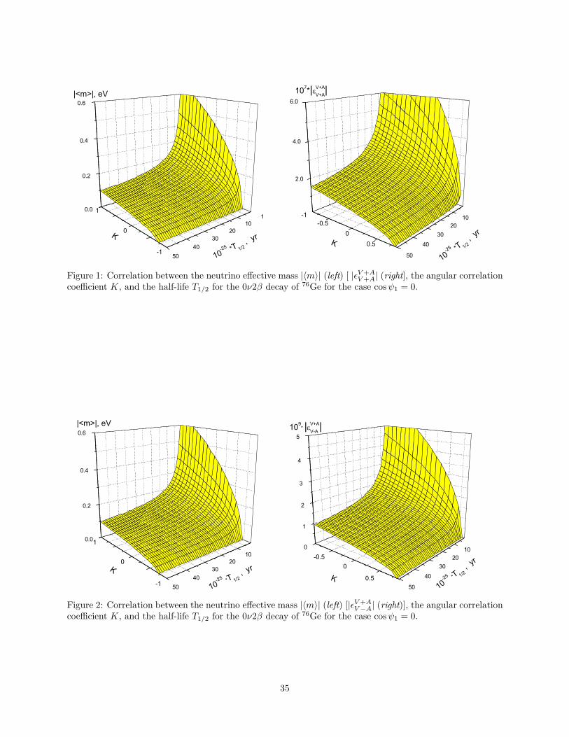
0.0
0.2
0.4
0.6
5040
3020
10
10-25 *T 1/2
, yrK
|<m>|, eV
-1
1
0
1
2.0
4.0
6.0
50
4030
2010
-0.5
10-25 *T 1/2
, yr
K 0
0.5
-1
107*| V+AV+A|
Figure 1: Correlation between the neutrino effective mass |〈m〉| (left) [ |ǫV +AV +A| (right], the angular correlation
coefficient K, and the half-life T1/2 for the 0ν2β decay of 76Ge for the case cosψ1 = 0.
0.0
0.2
0.4
0.6
5040
3020
10
|<m>|, eV
10-25 *T 1/2
, yrK
-1
1
0
0
1
2
3
4
5
50
4030
2010
10-25 *T 1/2
, yr
109* | V+A
V-A |
-0.5
0.5
0
K
Figure 2: Correlation between the neutrino effective mass |〈m〉| (left) [|ǫV+AV−A| (right)], the angular correlation
coefficient K, and the half-life T1/2 for the 0ν2β decay of 76Ge for the case cosψ1 = 0.
35
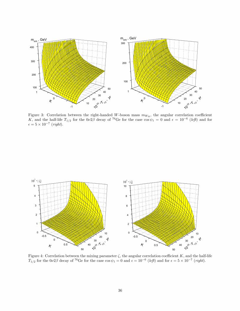
100
200
300
400
1020
3040
50
10-25 *T 1/2
, yr
K
-1
0
1
mWR , GeV
100
200
300
1020
3040
50
mWR , GeV
10-25 *T 1/2
, yr
K
-1
0
1
Figure 3: Correlation between the right-handed W -boson mass mWR , the angular correlation coefficientK, and the half-life T1/2 for the 0ν2β decay of 76Ge for the case cosψ1 = 0 and ǫ = 10−6 (left) and forǫ = 5× 10⁻⁷ (right).
0
1
2
3
4
5
50
4030
2010
*
10-25 *T 1/2
, yr
-0.5 0
0.5K
0
2
4
6
8
10
50
4030
2010
*
10-25 *T 1/2
, yr-0.5
K 0
0.5
Figure 4: Correlation between the mixing parameter ζ, the angular correlation coefficient K, and the half-lifeT1/2 for the 0ν2β decay of 76Ge for the case cosψ1 = 0 and ǫ = 10−6 (left) and for ǫ = 5× 10⁻⁷ (right).
36
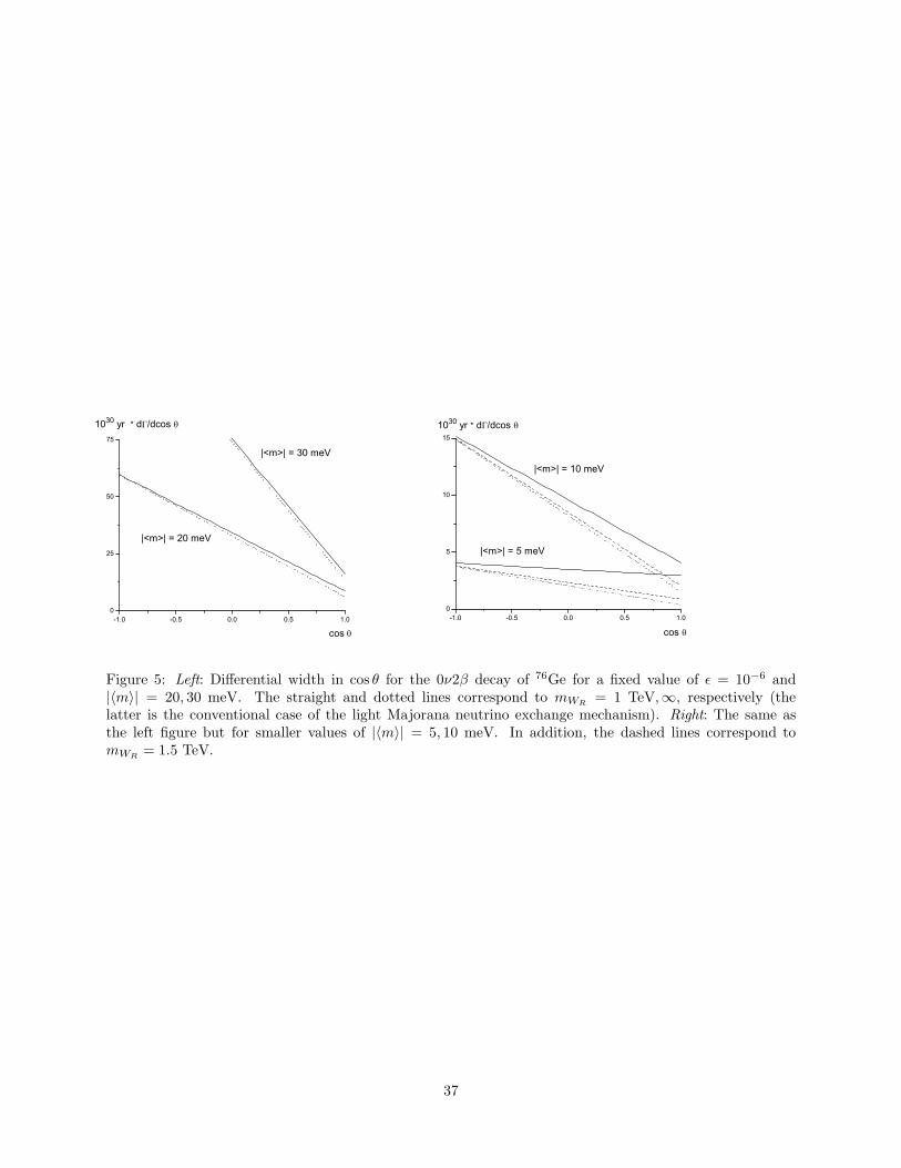
-1.0 -0.5 0.0 0.5 1.00
25
50
75
1030 yr * d /dcos
cos
|<m>| = 30 meV
|<m>| = 20 meV
-1.0 -0.5 0.0 0.5 1.00
5
10
15
|<m>| = 5 meV
cos
1030 yr * d /dcos
|<m>| = 10 meV
Figure 5: Left: Differential width in cos θ for the 0ν2β decay of 76Ge for a fixed value of ǫ = 10−6 and|〈m〉| = 20, 30 meV. The straight and dotted lines correspond to mWR = 1 TeV,∞, respectively (thelatter is the conventional case of the light Majorana neutrino exchange mechanism). Right: The same asthe left figure but for smaller values of |〈m〉| = 5, 10 meV. In addition, the dashed lines correspond tomWR = 1.5 TeV.
37