Finance and Economics Discussion Series

Federal Reserve Board, Washington, D.C.ISSN 1936-2854 (Print)

ISSN 2767-3898 (Online)

Desperate House Sellers: Distress Among Developers

Eileen van Straelen

2021-065

Please cite this paper as:van Straelen, Eileen (2021). “Desperate House Sellers: Distress Among Developers,” Financeand Economics Discussion Series 2021-065. Washington: Board of Governors of the FederalReserve System, https://doi.org/10.17016/FEDS.2021.065.

NOTE: Staff working papers in the Finance and Economics Discussion Series (FEDS) are preliminarymaterials circulated to stimulate discussion and critical comment. The analysis and conclusions set forthare those of the authors and do not indicate concurrence by other members of the research staff or theBoard of Governors. References in publications to the Finance and Economics Discussion Series (other thanacknowledgement) should be cleared with the author(s) to protect the tentative character of these papers.

Desperate House Sellers: Distress Among Developers

21st July 2021

Abstract

Using granular data on home builder housing developments from the 2006-09 housing

crisis, I show that builders spread house price shocks across geographically distinct projects

via their internal capital markets. Builders who experience losses in one area subsequently

sell homes in unaffected areas at a discount to raise cash quickly. Financially constrained

firms are more likely to cut prices of homes in healthy areas in response to losses in unhealthy

ones. Firms also smooth shocks across projects only during the crisis and not during the

boom. These results together suggest firm internal capital markets spread negative economic

shocks across space.

1

1 Introduction

Financial frictions can negatively affect economic activity. These frictions prevent firms from

accessing external funds, forcing them to rely on internal cash flows (Myers and Majluf, 1984).

From 2003-2009, internal funds made up 85% of total corporate financing.1 When firms rely

on internal financing, shocks to one part of the firm can propagate to other parts.2 These

within-firm spillovers are important because they cause firms to reduce investment in positive

NPV projects when financing constraints bind.3 These spillovers also indicate that economic

activity in different industries is linked through firms’ internal networks. But evidence of

within-firm spillovers affecting prices is limited.4 I present new findings on within-firm price

spillovers using granular data on the geographically distinct housing developments of home

builders. I show that during the 2006-09 housing crisis, when builders lost money on one

project, they cut prices on homes they had for sale in healthy, geographically distant projects

in order to speed up sales and generate cash quickly.

The home building industry provides a natural laboratory to study internal capital mar-

kets, overcoming several of the empirical concerns that make investigating this subject dif-

ficult. One of these concerns is the inability to precisely measure projects and their NPVs

within a firm. Conglomerate segment data, which has been used extensively in the past, is

often imprecise and has been found inaccurate (Whited, 2001). A second concern is endo-

geneity. Investment across different projects within a firm may be correlated because firms

subsidize failing projects with funds from healthy ones, or because all projects are exposed

to the same economic shocks. For example, different firm projects will experience the same

1See the Board of Governors of the Federal Reserve System, Flow of Funds Accounts of the United States,Table F.103.

2There is a large literature on internal capital markets, including work by Gertner et al. (1994), Rajanet al. (2000), Scharfstein and Stein (2000), and Stein (1997). Early seminal works in this area include Alchian(1969) and Williamson (1975).

3See Lamont (1997), Peek and Rosengren (2000), Giroud and Mueller (2017), Mondragon (2018) andCetorelli and Goldberg (2012).

4See e.g. Ge (2017), described in Section 1.1.

2

shock if the projects are located in the same area and therefore share exposure to the same

local economic conditions (Chevalier, 2004). My approach addresses both these concerns be-

cause I use granular data on housing developments to identify firm projects. These projects

are geographically distinct and therefore vary in their exposure to the 2006-09 housing crisis.

I find that a 10% (∼ one standard deviation) decrease in the value of a builder’s projects

in other markets leads to a 2.2% decrease in her house prices in unaffected areas. Models of

internal capital markets suggest that firms tend to cross-subsidize projects when access to

external financing is costly. Consistent with these models, I find that financially constrained

builders are more likely to spread shocks across projects. I also find no effect during the

2002-05 housing boom, a period when financing constraints did not bind because builders

could easily obtain credit. I show that when builders cut prices they sell homes more quickly

and that builders spread price shocks more to areas where a price cut produces a larger

decline in time-to-sale.

To analyze this industry, I construct a unique dataset of builder home sales matched to

builder finances. I start with a Corelogic dataset of housing transactions, which records rich

information on the characteristics of homes, such as square footage and property type. I

use these variables to control for differences in home quality between builders that would

otherwise confound the results. Next, note that if builders cut prices in healthy areas due

to internal capital markets, then the tendency to cut prices should correlate with builder

financial constraints. To test this hypothesis, I construct a variety of measures of financial

constraints, some that are generic in the corporate finance literature and some that are

unique to the home building industry and merge these to builder home sales. Finally, to

investigate if constrained builders cut prices to speed up sales, I gather data from realtor

listings that report homes’ time on the market and merge these listings to home sales. The

resulting dataset reports a home’s location, price, quality, and time-to-sale, creating a novel

setting to study internal capital markets and prices.

To conduct my empirical analysis, I compare prices for observationally identical homes

3

sold in the same zip code and year by different builders who differ in their exposure to house

price shocks in other areas. I measure a builder’s exposure to price shocks as the weighted

average change in prices in counties where the builder operates, with weights that reflect the

importance of each county in the builder’s overall portfolio. If I were to evaluate the effect

of a builder losing money in a given county on the builder’s pricing in that same county,

then any effect I find would be contaminated by local economic conditions. In contrast, in

my empirical design I separate local economic conditions from the builder’s condition by

evaluating a constrained builder’s pricing in a region separate from the one in which the

builder initially lost money. The effect is likely an underestimate because when shocked

builders cut prices, the prices of non-shocked builder homes may fall due to comparable

pricing.5 To test this, I show that when builders sell homes at a discount, the prices of

nearby, non-builder resale homes decline. In addition, the effect increases when I compare

the pricing of shocked and non-shocked builders within small time frames where comparable

pricing matters less.

The validity of my analysis rests on the assumption that a builder’s initial decision to

build in a housing bust area is independent of his potential pricing.6 This assumption will be

violated if the house price shock affects all regions and the builders who located in bust areas

serve a clientele more negatively affected by the common shock. To address this problem, I

perform a number of tests. First, if builders with exposure to bust markets, (shocked), cater

to a different clientele than builders without that exposure, (non-shocked), then I would

expect these builders to also differ in pricing before the 2006-09 crisis. To test this, I show

graphically that pricing for shocked and non-shocked builders only diverges during the crisis

period and not before. Second, if shocked builders sold to a different socio-economic group,

then there should be a difference in the luxury, quality, and neighborhood of the homes these

5See Campbell et al. (2011) and Guren (2018).6The housing bust period refers to years 2006-09 and the housing boom period refers to years 2002-05

throughout.

4

builders sell. To address this possibility, I show the effect remains robust to controlling for

zip code by year fixed effects and a host of variables describing home quality.

1.1 Related Literature

My results contribute to a broad literature in corporate finance on internal capital markets.

Papers in this area show that internal capital markets affect investment (Lamont, 1997),7

employment (Giroud and Mueller, 2017), and lending (Peek and Rosengren, 2000). Ge

(2017) also studies how internal capital markets affect prices but focuses specifically on the

life insurance industry, showing that distressed insurers lower premiums on contracts that

increase firm capital. Little is known about the effect of internal capital markets on prices

in durable goods industries, where buyers and sellers face search frictions and sellers must

invest time to find a buyer with a high value for their good. I show in the home builder

industry that firms respond to a loss in one project by slashing prices in geographically

distant projects, and I use detailed time-to-sale data from listings records to show that firms

cut prices to speed up sales. My findings have implications for price contagion in other

durable goods industries, such as the automobile and household goods industries.

In addition, my findings contribute to a growing literature on the propagation of lo-

cal geographic shocks (Bailey et al., 2017; Benmelech et al., 2014; Campbell et al., 2011;

DeFusco et al., 2018; Notowidigdo, 2011). Giroud and Mueller (2017) show that when a

negative economic shock affects one branch of a firm, the firm cuts employment in other,

geographically distant branches. I also show that firms spread negative economic shocks

across geography via their internal networks, but my paper has several important differences

from theirs. First, whereas Giroud and Mueller (2017) study employment, I study pricing,

a new margin of geographic contagion. Second, Giroud and Mueller (2017) do not observe

data on firm clientele, leaving them less able to address the concern that a firm cuts employ-

7See also Berger and Ofek (1995), Lang and Stulz (1994), and Shin and Park (1999).

5

ment in an unaffected project because the firm’s clientele has reduced demand. In contrast,

I have granular data on the physical characteristics of homes that builders sell which I use to

capture clientele differences between builders which would otherwise confound the results.

I also contribute to the literature on financial distress and prices. (Benmelech and

Bergman, 2008, 2009, 2011; Ortiz-Molina and Phillips, 2010; Pulvino, 1998). Theory sug-

gests that distressed firms, unable to access external finance, sell equipment at a discount

to industry outsiders in order to raise cash quickly (Bernanke and Gertler, 1989; Kiyotaki

and Moore, 1997; Shleifer and Vishny, 1992, 2011). I add to this literature by connecting

fire sales to internal capital markets. I show that builders do not restrict fire sale behavior

to a single floundering project, but also sell off assets from healthy, unrelated projects when

in distress. This paper is also related to the literature on the effects of financial distress

on inventory prices. Other work has studied this relationship for supermarkets, (Chevalier,

1995), consumer goods, (Kim, 2018), and goods underlying the PPI (Gilchrist et al., 2017).

Using granular data on product quality, price, and time-to-sale, I show in a durable goods

industry that distressed firms discount prices on inventory in order to make sales quickly.

Lastly, my findings add to a literature on home builders in a housing downturn. Haugh-

wout et al. (2012) and Nathanson and Zwick (2017) show that during the last housing boom,

home builders over-developed and created an excess supply of homes, fueling the subsequent

bust in house prices. My results provide evidence that home builders further contribute to

housing downturns by cutting home prices in unaffected regions.

2 Home Building Overview

2.1 Home Building Business Landscape

The home building industry is an important part of the U.S. economy. In 2017, 13% of

homes sales were of newly constructed homes, with a total market size of roughly $236

6

billion. During the last housing boom the industry was even larger; in 2005, at a market size

of approximately $381 billion, it was responsible for 20% of home sales.8 However, despite

its considerable size, the industry is also fragmented, with a few large firms and many small

builders. In 2007, the U.S. Economic Census reported a total of 98,067 home builders. These

builders range from large, publicly traded firms producing thousands of homes a year, to

one-person contractors hired by a home buyer to build a home to their specification. Indeed,

in 2007, 65% of home builders had sales receipts of less than $1 million. In this paper, I focus

on the large home building firms for two main reasons. First and foremost, small contractors

are unlikely to have more than one home on the market at any one time, and therefore would

not exhibit any kind of cross subsidizing behavior across distinct developments. Furthermore,

small builders are not geographically dispersed enough for their separate housing projects to

experience different shocks.9

Builders’ housing developments are constructed separately from each other and take

three to five years to develop. Builders buy land, develop the parcels, hire subcontractors

to construct homes on the parcels, and then sell those homes directly to households via

their in-house real estate agents. Builders construct both made-to-order and ready-made

homes, called “speculative” homes. Once a contract for a made-to-order home with a home

buyer is struck, the builder hires subcontractors to build the home to the preferences of the

buyer. Consequently, builder inventory consists mostly of tracts of land and partially and

fully completed homes. Builders often purchase land parcels using options, giving them the

right to buy the land outright at a certain price within a given time. Option prices tend

to be around 10% of the actual land value. When land values plummeted during the crisis,

builders with more of their land owned via options rather than owned outright should have

enjoyed a stronger financial position.

8See the U.S. Census, New Residential Sales, the Department of Housing and Urban Development, andthe National Association of Realtors.

9The large builders make up approximately 25% of new home sales in 2009.

7

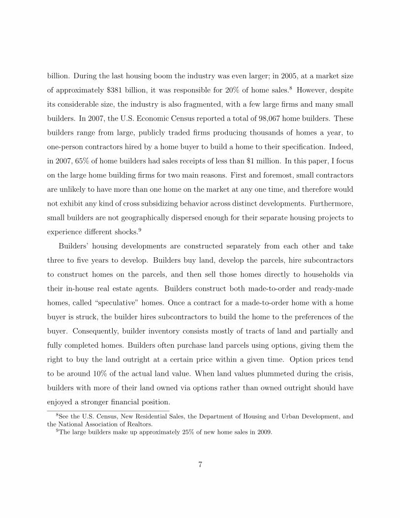
The large home builders have wide geographic dispersion. To illustrate this, Figure 1

reports the concentration in 2009 across U.S. counties of homes sold by the builders in my

sample in 2009. Builders operated in the West, Southwest, and along the eastern seaboard,

areas which experienced very different house price trajectories during the last crisis. My

sample, which is described in detail in Section 4, contains roughly 2,000 large builders. Table

I reports summary statistics on the geographic dispersion of these builders. In this sample,

the average builder sells 72 homes per year and operates in approximately 3 different states.

The number of states a builder builds homes in is not a complete measure of geographic

spread, since a builder may technically operate in two states but sell 99% of his homes in

one state, and 1% in the second. To get a better sense of a builder’s concentration across

states, I construct a geographic HHI equal to the squared sum of the fraction of homes a

builder sells in each state. The average builder in my sample has an HHI of 0.51, suggesting

equal concentration across two states. Public home builders are larger and more dispersed

than private ones; the average public home builder sells 4,265 homes per year and operates

in 14 states.

2.2 Home Building Financing

This paper focuses on large builders, defined as selling more than two homes per year and

operating in more than one county. The analysis of builder finances focuses on the subset of

large builders which are publicly traded and therefore report financial information. Public

builders finance themselves using cash from operations, unsecured public debt, revolving

credit facilities, mortgage notes, and operating leases. In Table I, I report summary statistics

on builder financing taken from the annual reports of public builders. Large public builders

have an average leverage ratio of 0.39, defined as the ratio of total debt to total assets.

From the 1970s, when the large home builder industry arose, until 2007, land prices had

8

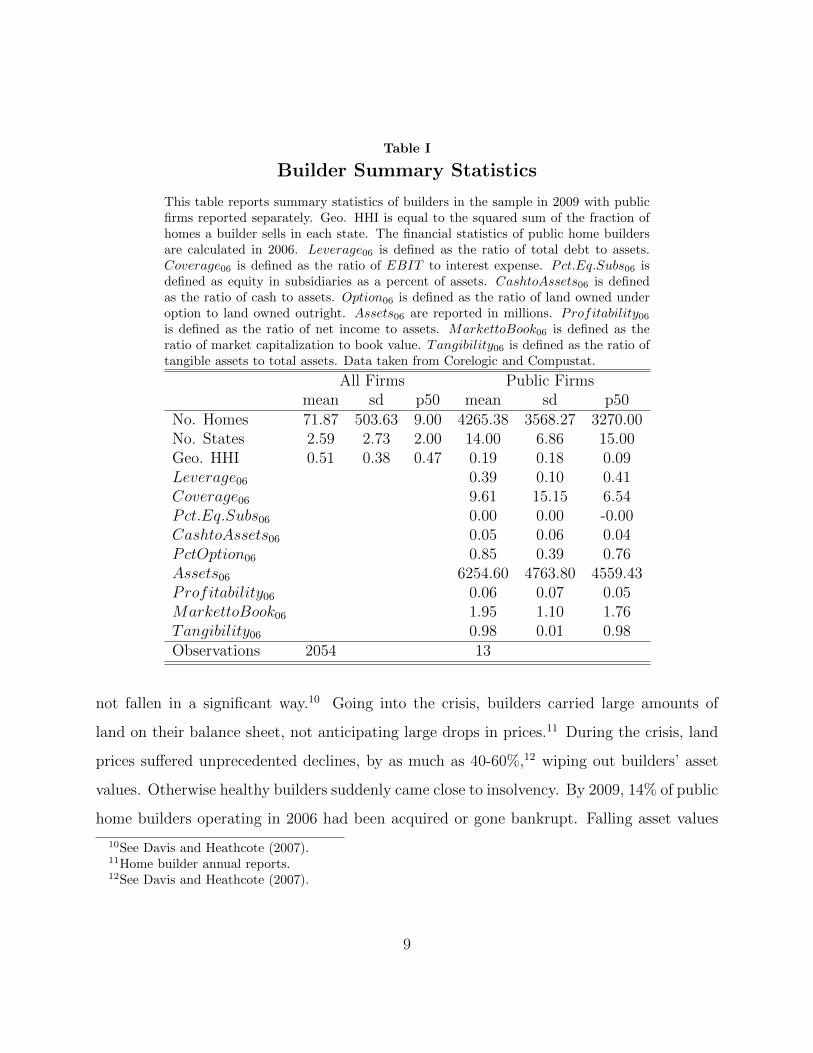
Table I

Builder Summary Statistics

This table reports summary statistics of builders in the sample in 2009 with publicfirms reported separately. Geo. HHI is equal to the squared sum of the fraction ofhomes a builder sells in each state. The financial statistics of public home buildersare calculated in 2006. Leverage06 is defined as the ratio of total debt to assets.Coverage06 is defined as the ratio of EBIT to interest expense. Pct.Eq.Subs06 isdefined as equity in subsidiaries as a percent of assets. CashtoAssets06 is definedas the ratio of cash to assets. Option06 is defined as the ratio of land owned underoption to land owned outright. Assets06 are reported in millions. Profitability06is defined as the ratio of net income to assets. MarkettoBook06 is defined as theratio of market capitalization to book value. Tangibility06 is defined as the ratio oftangible assets to total assets. Data taken from Corelogic and Compustat.

All Firms Public Firmsmean sd p50 mean sd p50

No. Homes 71.87 503.63 9.00 4265.38 3568.27 3270.00No. States 2.59 2.73 2.00 14.00 6.86 15.00Geo. HHI 0.51 0.38 0.47 0.19 0.18 0.09Leverage06 0.39 0.10 0.41Coverage06 9.61 15.15 6.54Pct.Eq.Subs06 0.00 0.00 -0.00CashtoAssets06 0.05 0.06 0.04PctOption06 0.85 0.39 0.76Assets06 6254.60 4763.80 4559.43Profitability06 0.06 0.07 0.05MarkettoBook06 1.95 1.10 1.76Tangibility06 0.98 0.01 0.98Observations 2054 13

not fallen in a significant way.10 Going into the crisis, builders carried large amounts of

land on their balance sheet, not anticipating large drops in prices.11 During the crisis, land

prices suffered unprecedented declines, by as much as 40-60%,12 wiping out builders’ asset

values. Otherwise healthy builders suddenly came close to insolvency. By 2009, 14% of public

home builders operating in 2006 had been acquired or gone bankrupt. Falling asset values

10See Davis and Heathcote (2007).11Home builder annual reports.12See Davis and Heathcote (2007).

9

(213,5195](43,213](8,43][1,8]No data

Figure 1. Builder geographic dispersion. This figure shows the geographic distribution of homes soldby the 2,054 builders in the main sample in 2009.

effectively cut off many builders from external financing during the crisis. Builders were

forced to rely on internally generated funds. This led them to sell off assets at a discount.13

Builders explicitly discuss their difficulty in accessing financing during the crisis in their

annual reports. D.R. Horton, one of the three largest public home builders in the U.S., writes

in its 2009 10-k:

“During this downturn in the home building industry, we have relied principally on the pos-

itive operating cash flow we have generated to meet our working capital needs and repay

outstanding indebtedness. We generated substantial operating cash flow during this time.

However, the downturn and the constriction of the credit markets have reduced the other

sources of liquidity available to us and increased our costs of capital.”

This is followed by a desire to sell off assets quickly:

“In light of the challenging home building market conditions experienced over the past few

years, we have been operating with a primary focus to generate cash flows through reduction

13Home builder annual reports.

10

in assets.”

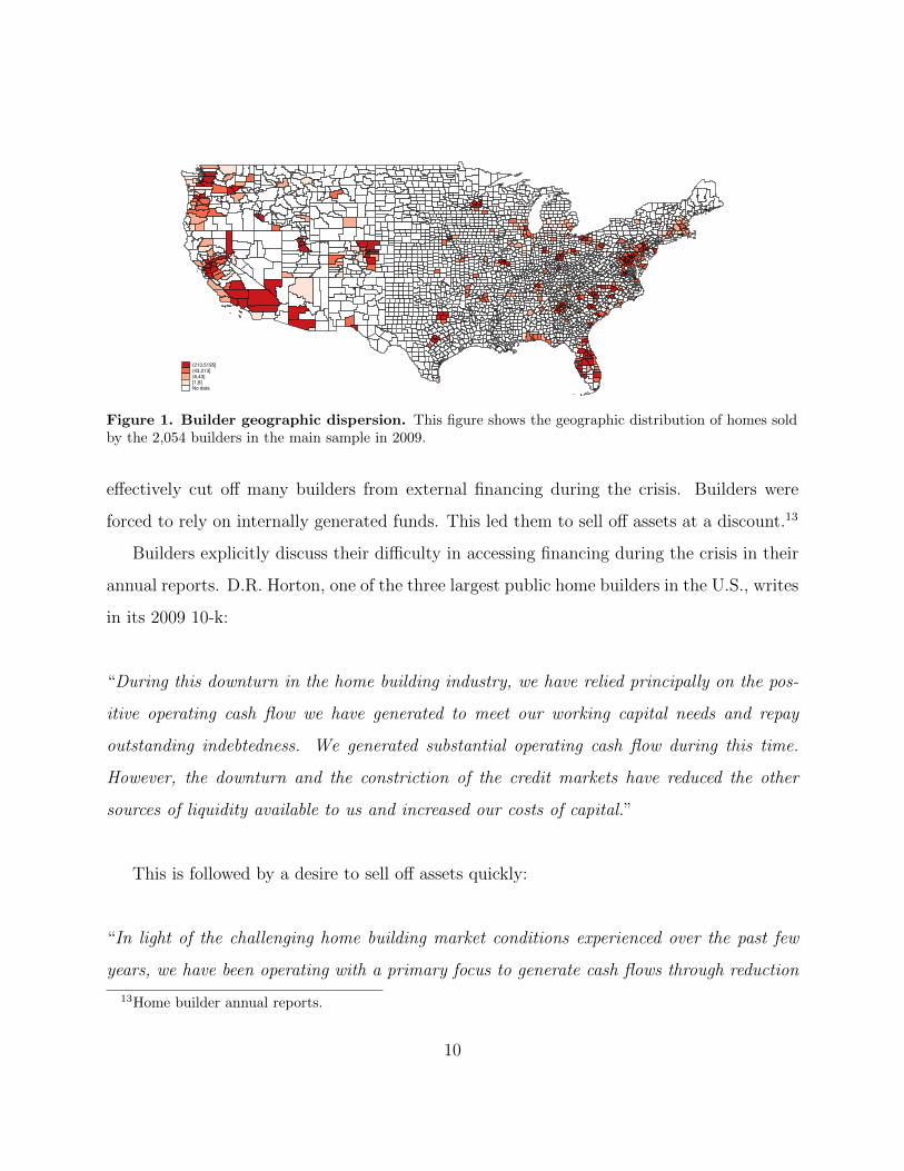
The credit crisis occurred simultaneously with an extreme reversal of economic fortune

for builders. In the run up to 2007, builders competed with each other to buy land in

hot markets like Las Vegas. The ensuing housing bust in those areas led to severe asset

impairments and sell-offs for builders holding that land. The right panel of Figure 2 plots

this decline, in which builder asset values peak in 2005 and then plummet between 2007 and

2010. As the annual reports make clear, builders responded to the decline in land values by

rapidly selling off land to build up cash reserves. The left panel of Figure 2 plots these steep

changes in builder cash: builders begin to dramatically accumulate cash beginning in 2006,

with cash holdings peaking in 2009.

0200

400

600

800

Cash $

(Mil)

2000 2002 2004 2006 2008 2010 2012 2014Year

(a) Panel A: Home Builder Cash

2000

3000

4000

5000

Assets

$(M

il)

2000 2002 2004 2006 2008 2010 2012 2014Year

(b) Panel B: Home Builder Assets

Figure 2. Home builder cash and assets. This figure plots average cash and assets between 2001 and2015 for the group of public home builders. All data taken from Compustat.

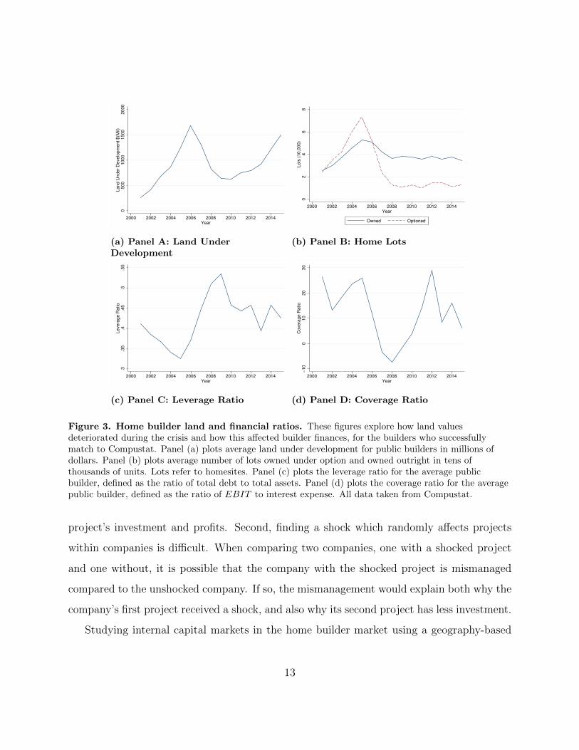
Figure 3 illustrates how declining land values contributed to a deteriorating financial

condition for builders. The upper left panel plots land under development over time. Land

under development peaks in 2006 and falls by more than half in 2008. This decline should

reflect three factors: builders selling off land, land value impairments, and builders choosing

11

to postpone development of their holdings. Lots owned and lots optioned, (shown in the

upper right panel), follow this behavior, as both lots owned and lots optioned peak in 2005

before falling sharply. Lots optioned rose more quickly in the boom and also fell more quickly

in the bust than lots owned outright. Since options are easier to dispense with than land, this

suggests builders may have preferred to sell off more land during the crisis than they actually

did. The decline in land values led to a dramatic increase in the leverage ratio of builders

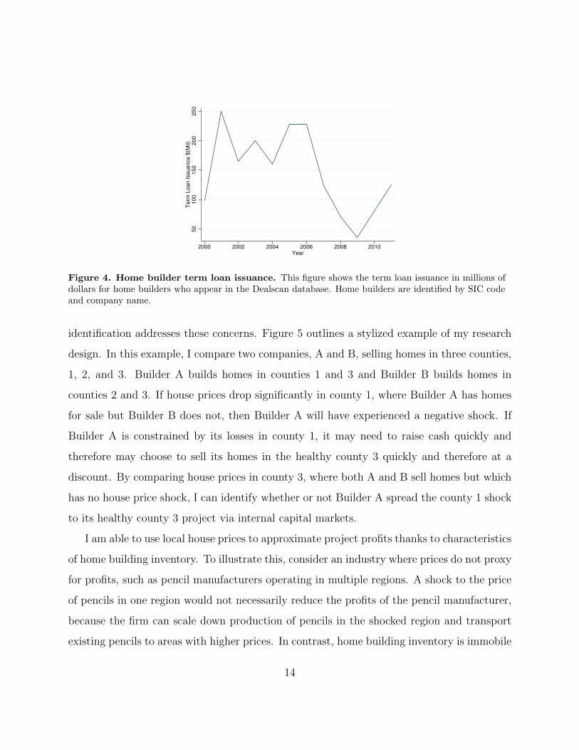
from 2005 to 2009, shown in the bottom left panel of Figure 3. The increase in leverage is all

the more striking because builders stopped issuing debt, as Figure 4 illustrates. The overall

leverage increase implies that the decline in builder asset values overwhelmed the decline in

debt issuance. Lastly, the bottom right panel of Figure 3 plots the average builder coverage

ratio over time, defined as the ratio of EBIT to interest expense. The coverage ratio proxies

for a firm’s ability to service its debt out of cash flow. Higher values indicate a healthier

financial position. The average coverage ratio becomes negative in 2008, reflecting the fact

that the average builder was making a loss during the crisis. Together, these figures suggest

that the decline in land prices damaged builders’ finances, effectively cutting them off from

external financing.

3 Identification Strategy

An ideal experiment to test internal capital markets would compare two identical companies,

each operating multiple projects, and would randomly assign a negative revenue shock to one

of the projects. Finding that the company with the shocked project diverts investment from

its unshocked project to its shocked project, while the company with all unshocked projects

makes no adjustment, is evidence of internal capital markets at work. Approximating this

experiment in the real world is difficult due to data limitations and endogeneity concerns.

First, most public firms do not report project-level investment. Therefore it is challenging

to identify what constitutes an independent project within a firm, and to measure each

12

05

00

10

00

15

00

20

00

La

nd

Un

de

r D

eve

lop

me

nt

$(M

il)

2000 2002 2004 2006 2008 2010 2012 2014Year

(a) Panel A: Land UnderDevelopment

02

46

8L

ots

(1

0,0

00

)

2000 2002 2004 2006 2008 2010 2012 2014Year

Owned Optioned

(b) Panel B: Home Lots

.3.3

5.4

.45

.5.5

5L

eve

rag

e R

atio

2000 2002 2004 2006 2008 2010 2012 2014Year

(c) Panel C: Leverage Ratio

−1

00

10

20

30

Co

ve

rag

e R

atio

2000 2002 2004 2006 2008 2010 2012 2014Year

(d) Panel D: Coverage Ratio

Figure 3. Home builder land and financial ratios. These figures explore how land valuesdeteriorated during the crisis and how this affected builder finances, for the builders who successfullymatch to Compustat. Panel (a) plots average land under development for public builders in millions ofdollars. Panel (b) plots average number of lots owned under option and owned outright in tens ofthousands of units. Lots refer to homesites. Panel (c) plots the leverage ratio for the average publicbuilder, defined as the ratio of total debt to total assets. Panel (d) plots the coverage ratio for the averagepublic builder, defined as the ratio of EBIT to interest expense. All data taken from Compustat.

project’s investment and profits. Second, finding a shock which randomly affects projects

within companies is difficult. When comparing two companies, one with a shocked project

and one without, it is possible that the company with the shocked project is mismanaged

compared to the unshocked company. If so, the mismanagement would explain both why the

company’s first project received a shock, and also why its second project has less investment.

Studying internal capital markets in the home builder market using a geography-based

13

50

10

01

50

20

02

50

Te

rm L

oa

n I

ssu

an

ce

$(M

il)

2000 2002 2004 2006 2008 2010Year

Figure 4. Home builder term loan issuance. This figure shows the term loan issuance in millions ofdollars for home builders who appear in the Dealscan database. Home builders are identified by SIC codeand company name.

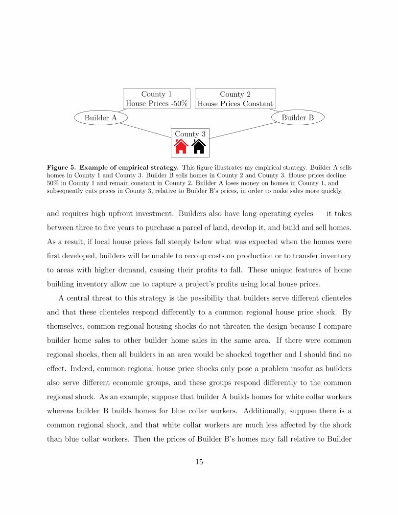
identification addresses these concerns. Figure 5 outlines a stylized example of my research

design. In this example, I compare two companies, A and B, selling homes in three counties,

1, 2, and 3. Builder A builds homes in counties 1 and 3 and Builder B builds homes in

counties 2 and 3. If house prices drop significantly in county 1, where Builder A has homes

for sale but Builder B does not, then Builder A will have experienced a negative shock. If

Builder A is constrained by its losses in county 1, it may need to raise cash quickly and

therefore may choose to sell its homes in the healthy county 3 quickly and therefore at a

discount. By comparing house prices in county 3, where both A and B sell homes but which

has no house price shock, I can identify whether or not Builder A spread the county 1 shock

to its healthy county 3 project via internal capital markets.

I am able to use local house prices to approximate project profits thanks to characteristics

of home building inventory. To illustrate this, consider an industry where prices do not proxy

for profits, such as pencil manufacturers operating in multiple regions. A shock to the price

of pencils in one region would not necessarily reduce the profits of the pencil manufacturer,

because the firm can scale down production of pencils in the shocked region and transport

existing pencils to areas with higher prices. In contrast, home building inventory is immobile

14

County 1House Prices -50%

County 3

County 2House Prices Constant

Builder A Builder B

Figure 5. Example of empirical strategy. This figure illustrates my empirical strategy. Builder A sellshomes in County 1 and County 3. Builder B sells homes in County 2 and County 3. House prices decline50% in County 1 and remain constant in County 2. Builder A loses money on homes in County 1, andsubsequently cuts prices in County 3, relative to Builder B’s prices, in order to make sales more quickly.

and requires high upfront investment. Builders also have long operating cycles — it takes

between three to five years to purchase a parcel of land, develop it, and build and sell homes.

As a result, if local house prices fall steeply below what was expected when the homes were

first developed, builders will be unable to recoup costs on production or to transfer inventory

to areas with higher demand, causing their profits to fall. These unique features of home

building inventory allow me to capture a project’s profits using local house prices.

A central threat to this strategy is the possibility that builders serve different clienteles

and that these clienteles respond differently to a common regional house price shock. By

themselves, common regional housing shocks do not threaten the design because I compare

builder home sales to other builder home sales in the same area. If there were common

regional shocks, then all builders in an area would be shocked together and I should find no

effect. Indeed, common regional house price shocks only pose a problem insofar as builders

also serve different economic groups, and these groups respond differently to the common

regional shock. As an example, suppose that builder A builds homes for white collar workers

whereas builder B builds homes for blue collar workers. Additionally, suppose there is a

common regional shock, and that white collar workers are much less affected by the shock

than blue collar workers. Then the prices of Builder B’s homes may fall relative to Builder

15

A’s, because Builder B’s clients, responding to the common shock, decrease their demand

for homes whereas Builder A’s clients are unaffected and their demand remains constant.

To address this problem, my analysis will exploit the rich geographic and structural detail

in the Corelogic housing transactions dataset.14 I restrict to home sales made in 2009 and

use zip code fixed effects to compare homes sold within the same zip code and year. I also

control for observables of the home, such as square footage and bathrooms.15 It is unlikely

that structurally similar homes, on the market in the same zip code and in the same year,

sell to different classes of customer.

I also address this problem by testing a specification which makes it less likely that a

builder’s shock is common to all regions. To do this, I calculate a builder’s shock using only

geographically distant counties. In particular, in robustness checks I generate results in which

a builder j’s county k-specific shock is calculated excluding house price changes occurring in

counties in the same state as county k. This analysis excludes builders operating in multiple

counties within a single state, and therefore the sample size falls. Despite the smaller number

of observations, the results are similar when using this more geographically distinct definition

of a builder’s exposure to other regions.

Of course, the decision of where to initially build developments is not randomly assigned.

Builders choose locations based on proximity to headquarters, projections for income and

population growth, and local land use regulations. The validity of my analysis rests on the

assumption that builders’ decisions to build in certain states during the housing boom period

do not correlate with their potential pricing in 2009, conditional on physical and geographic

characteristics of homes. In robustness checks I test the validity of this assumption by

showing that exposed and unexposed builders’ pricing follow parallel trends before the crisis.

Another potential threat is the possibility that builder geographic networks overlap with

14I describe the Corelogic dataset in detail in Section 4.15In robustness checks I control for zip code fixed effects interacted with home characteristics, to allow the

effect of home quality to vary by zip code, and find the results do not change.

16

networks of other agents, such as lenders, who may also spread shocks across geography

(Mondragon, 2018; Gilje et al., 2016; Cortes and Strahan, 2017). I address this threat

in my design because I compare homes selling within the same zipcode and year. If a

lender experiences losses in a housing bust area and transmits those losses to healthy areas

by cutting lending, then shocked and non-shocked builders in the healthy area should be

equally affected; a credit shock common to an entire zipcode cannot explain differential

pricing between builders within the same zipcode.

4 Data and Summary Statistics

For my analysis I merge home sales transactions to home builders’ finances and home listing

records. This section discusses the merging of the data and the construction of the variables

used in the paper.

My main source of data is the tax and deed databases from Corelogic. Corelogic is

a private company specializing in real estate data; they compile public records of housing

transactions and property tax assessments from U.S. county recorder offices. Corelogic’s deed

database records, for each house purchase, the seller name, buyer name, and detailed address

information. The Corelogic tax database consists of tax assessments made against homes;

these include information on home quality such as repairs and additions, as well as a variety

of details on homes’ structural characteristics. I merge the home purchase information from

the deed database to the house characteristics’ information in the tax database to create a

dataset of housing transactions with physical characteristics of homes.

Next, I impose a number of filters on the data in order to create a sample representative

of the U.S. new home market.16 First, I restrict to arms length transactions only. This

16Builder inventory mostly consists of homes and land lots. When builders are in distress, they may sell offland, in addition to homes, at a discount to raise cash quickly. When builders are in distress, the tendencyto make discounted sales may be stronger for land than for homes. To see why, recall that if a builder cutsprices on homes today, this will adversely impact the prices of homes he sells in the future, because homes

17

excludes, for example, home sales made between family members or spouses, which may

have distorted pricing. I further restrict to single family, condominium, and duplex homes.

I exclude foreclosure sales and any transactions made against the home (such as refis or

HELOCs), which do not represent a house purchase. I identify unique homes using the

Assessor’s Parcel Number (APN) variable, the APN sequence number, and county code.

The APN variable is created by the county recorder to identify unique homes. The APN

sequence number is an additional county variable used to ensure a home’s uniqueness in

conjunction with the APN variable. I then drop duplicate sales, in which the seller, buyer,

APN identifier, APN sequence number, county code, and sale amount are the same.

Within this sample of arms length transactions, I identify a subsample of sales of newly

constructed homes. I first restrict to homes built after 2000, to ensure the homes are in fact

recently built. This sample includes first as well as resales of new homes; I then restrict to

only the first sales of new homes.17 To validate my identification of new home sales, I compare

my data to new housing permits from the Census in Appendix Figure 10. I next clean the

seller name field using various string matching algorithms. String cleaning methods are not

sufficient to completely group homes to builders however, because several large builders sell

homes under subsidiary name brands. To ensure that I group together homes sold by the

same company but under different brand names, I manually match subsidiary builder names

to parent builder names for the public builders and largest private builders. I validate my

assignment of homes to builders using industry data in Appendix Figure 11.

To focus on home builders of reasonable size, I remove builders who sell no more than

two homes per year. To focus on builders with sufficient geographic dispersion, I require that

builders sell homes in more than one county. These restrictions narrow the sample to 98,151

are priced off sales of comparable homes. This pricing effect is not at play for land sales, which suggestsconstrained builders have more of an incentive to cut land as opposed to home prices. Unfortunately, detailedland sale data is not available in Corelogic.

17I use the APN variable to group together sales of the same home over time. Within the resulting panels,I classify the first transaction made against the home as the new home purchase.

18

home sales, corresponding to approximately 25% of new homes sales made in the U.S. in

2009. These home sales are made by a total of 2,054 unique builders.

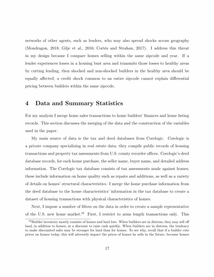
Table II reports summary statistics of the homes sold in this sample. The rich housing

characteristics that Corelogic provides, such as number of bathrooms and square footage, go

a long way towards determining the price of a home, and therefore are very useful controls

for home quality. The average home in my sample sells for $263,228 in 2009 dollars; for the

subset of homes sold by public builders, the mean home sells for $260,942. 92% of homes in

the sample are single family as opposed to condominiums. Large public builders often have

affiliated financing arms that offer mortgages to their customers. In 2009, builder mortgage

arms financed 32% of home sales in my sample. Corelogic reports additional controls, such

as fireplace type, roof type, and condition type, but these variables are not populated for a

large fraction of homes. Including all variables makes the sample size drop significantly, so

I do not use them in the main specification. Nonetheless, I show in robustness checks that

the results remain similar when these variables are included.

I use the updated seller name field to merge builder homes to builder financial information

from Compustat, Dealscan, and SDC Platinum. I obtain from Compustat builder financial

information as well as variables specific to home builders, such as lots owned, lots owned

under option, land under development, and equity in unconsolidated subsidiaries. I use

Compustat to construct the leverage ratio of a firm, which I define as the ratio of total debt

to assets. I also use Compustat to construct a builder’s coverage ratio, defined as the ratio

of EBIT to interest expense. I am able to obtain financial information from Compustat

for 33 home builders over the period 2001-2015. However, in 2009, only 13 builders report

finances in Compustat. I use Dealscan to obtain syndicated bank loan issuances for both

public and large private home builders. I use SDC Platinum to obtain information on public

bond issuances of builders. Lastly, I use the Zillow House Price Index for county level house

prices.

For time-to-sale information, I use Corelogic’s Multiple Listing Service (MLS) dataset,

19

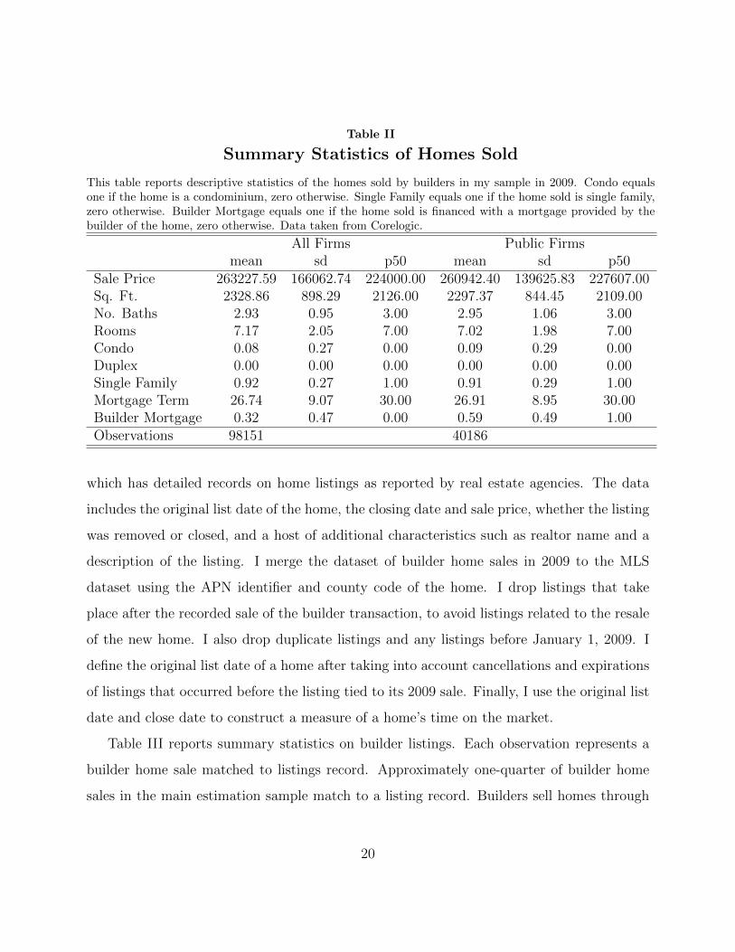
Table II

Summary Statistics of Homes Sold

This table reports descriptive statistics of the homes sold by builders in my sample in 2009. Condo equalsone if the home is a condominium, zero otherwise. Single Family equals one if the home sold is single family,zero otherwise. Builder Mortgage equals one if the home sold is financed with a mortgage provided by thebuilder of the home, zero otherwise. Data taken from Corelogic.

All Firms Public Firmsmean sd p50 mean sd p50

Sale Price 263227.59 166062.74 224000.00 260942.40 139625.83 227607.00Sq. Ft. 2328.86 898.29 2126.00 2297.37 844.45 2109.00No. Baths 2.93 0.95 3.00 2.95 1.06 3.00Rooms 7.17 2.05 7.00 7.02 1.98 7.00Condo 0.08 0.27 0.00 0.09 0.29 0.00Duplex 0.00 0.00 0.00 0.00 0.00 0.00Single Family 0.92 0.27 1.00 0.91 0.29 1.00Mortgage Term 26.74 9.07 30.00 26.91 8.95 30.00Builder Mortgage 0.32 0.47 0.00 0.59 0.49 1.00Observations 98151 40186

which has detailed records on home listings as reported by real estate agencies. The data

includes the original list date of the home, the closing date and sale price, whether the listing

was removed or closed, and a host of additional characteristics such as realtor name and a

description of the listing. I merge the dataset of builder home sales in 2009 to the MLS

dataset using the APN identifier and county code of the home. I drop listings that take

place after the recorded sale of the builder transaction, to avoid listings related to the resale

of the new home. I also drop duplicate listings and any listings before January 1, 2009. I

define the original list date of a home after taking into account cancellations and expirations

of listings that occurred before the listing tied to its 2009 sale. Finally, I use the original list

date and close date to construct a measure of a home’s time on the market.

Table III reports summary statistics on builder listings. Each observation represents a

builder home sale matched to listings record. Approximately one-quarter of builder home

sales in the main estimation sample match to a listing record. Builders sell homes through

20

their own offices within a development and advertise homes by listings on their websites,

often not using realtors. As a result, realtors often miss builder listings in MLS, leading to

the relatively low match rate between builder homes and listings. The average builder home

sells approximately six months after its original listing, and homes sold by public builders

sell slightly faster. Prices and home characteristics within the sample of homes that have a

listing record are similar to the prices and characteristics of homes in the larger estimation

sample described in Table II.

Table III

Summary Statistics of Home Listings

This table reports descriptive statistics of the listings of homes sold by builders in my sample in 2009. Condoequals one if the home is a condominium, zero otherwise. Single Family equals one if the home sold is singlefamily, zero otherwise. Time on the market is defined as the difference between listing date and closing date.Data taken from Corelogic.

All Firms Public Firmsmean sd p50 mean sd p50

Listing Time (Days) 166.24 145.31 127.00 124.07 99.80 100.00Sale Price 271524.17 159627.64 233025.00 265647.25 132711.53 235000.00Sq. Ft. 2449.48 954.21 2257.00 2429.00 895.20 2268.00No. Baths 2.99 1.09 3.00 3.01 1.44 3.00Condo 0.05 0.22 0.00 0.07 0.25 0.00Duplex 0.00 0.00 0.00 0.00 0.00 0.00Single Family 0.95 0.23 1.00 0.93 0.25 1.00Observations 23800 7053

5 Empirical Analysis & Results

5.1 Empirical Specification

My empirical strategy analyzes the effect of builder exposure to shocked regions on the prices

of builder homes in unshocked regions. I begin by constructing a measure of a builder’s

21

exposure to house price changes in distant counties in 2009.18 Suppose a builder j operates

in counties 1, . . . .., K in 2006. The shock to builder j, in month t in 2009, in county k, is

defined as the weighted average of the change in house prices between 2006 and 2009 in all

other counties 1, . . . , K the builder has homes in, excluding county k. The change in house

prices in a county is calculated using Zillow. The weights are the fraction of the number of

homes builder j has sold in 2006 in a given county r, over the total number of homes builder

j sold in 2006.

ω06,r,j =No.homes06,j,rNo.homes06,j

(1)

A negative shock indicates that a builder has recently sold a large proportion of her available

homes in areas where prices fell, and consequently is likely to have suffered losses.

The main specification is below:

Log(SalePricei,t,j,k,09) = β1

K∑r 6=k

ω06,r,j∆(HPr)06−09 + β2HPt,k + β3Xi + γs(i) + εi,t,j,k (2)

That is, I regress the log sale price of house i, sold in month t in 2009, in county k, by builder

j, on builder j’s shock measure, which is calculated excluding house prices in county k.19 20

For brevity, I denote the shock measure,∑K

r 6=k ω06,r,j∆(HPr)06−09, as ∆HP j,06−09. I include

controls HPt,k for log county level house prices each month.21 All specifications also include

18In robustness exercises I calculate a builder’s exposure to distant house price changes at the zip codelevel. Table XIX in the Appendix reports estimates using this measure, which are similar to using exposurecalculated at the county level.

19To focus on geographically very distinct counties, in robustness checks I generate results in which abuilder j’s county k-specific shock is calculated excluding house price changes occurring in the same stateas county k.

20In Equation 2 the outcome variable, house prices in 2009, overlaps with the final year of the shockmeasure, defined over 2006 to 2009, leaving open the possibility of reverse causality. I address this concernin Appendix Section 11.6 by re-estimating Equation 2 using house prices in 2010 as the outcome variable.

21To further control for local economic conditions, I also control for the change in the log of county levelhouse prices between 2006 and 2009. See Table XVIII of the Appendix.

22

zip code fixed effects, γs(i). Since I evaluate the effect only in 2009, zip code fixed effects are

equivalent to zip code by year fixed effects. This specification allows me to compare sales

of homes within a narrow geography and small time frame. Controls Xi include variables

describing the characteristics of the house i, including: number of bathrooms, square footage,

and property type (i.e., single family home, condo, or duplex). The geography fixed effects

coupled with the vector of structural controls go a long way towards fully describing the price

of the home. Standard errors are clustered at the county level throughout. In robustness

exercises in Appendix Section 11.5 I cluster at the builder level and find that the results are

similar.22

Before reviewing the results, I summarize the threats to validity for the design. First, it

is possible that the shock metric I define may not completely capture builder exposure to

ailing markets. I define a builder’s exposure to a region according to the number of homes a

builder sells there in 2006. However, if homes sold does not proxy well for inventory, then I

could mis-measure the shock. For example, if a builder has many homes on the market in Las

Vegas during the housing bust, she may in fact sell very few of those homes, because demand

has dried up. This builder’s asset values would have indeed dropped, but the builder’s shock

would not fall because the shock is calculated off of homes sold, not off of unsold inventory.

This will introduce observations into the analysis which have an incorrectly small shock value

and a large price response, which should bias the result downwards.

A related problem is the possibility that multiple county builders respond differently

to common regional shocks than single county builders. A single county builder has zero

exposure to other counties, and therefore will always have a shock of zero. During the crisis,

large multiple county builders, having at least some exposure to bust states, would often have

negative shocks. As a result, the shock could correlate with builder dispersion and hence with

22Equation 2 defines the outcome variable, house prices, in levels. A specification in levels can producebias if the outcome variable exhibits autocorrelation. To address this possibility, in the Appendix I estimatea specification in first differences and find the results remain similar.

23

builder size. If large builders happen to respond differently to common shocks than small

builders, then any effect found could be due to builder size rather than to internal capital

markets. To address this concern, I restrict the sample to homes sold by large, multiple

county builders.

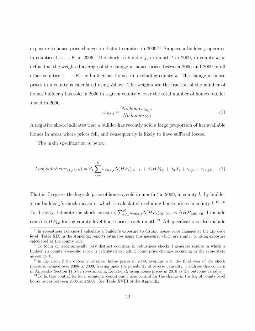
5.2 Results

Table IV presents results from Equation 2. β1 from Equation 2 is reported in the first row

along with its standard errors. Each column of the table corresponds to a specification with

a different set of housing characteristic controls. All specifications include zip code fixed

effects and log county level monthly house prices. The sample period corresponds to 2009,

and the shock is calculated over 2006-2009. Interpreting the coefficient from column 1, I

find that builders exposed to a negative 10% shock, (roughly one standard deviation of the

shock), sell homes for roughly 4% less than unexposed peers in 2009. As I add controls to

this specification, namely for square footage, bathrooms, and property type, the coefficient

falls somewhat in magnitude and remains stable in significance. In the most restrictive

specification in column 4, the coefficient implies that builders exposed to a negative 10%

shock sell homes for 2.2% less than unexposed peers. In columns 5 and 6 I restrict to the

subset of homes sold by public builders. In this smaller sample the standard errors increase

but the effect remains. The fact that the coefficient declines when adding property-specific

controls suggests that without the rich housing characteristics, I would likely be picking up

clientele differences between builders in addition to internal capital markets behavior.23

These results indicate that constrained builders cut inventory prices. Prior work by

Chevalier (1995) shows an opposite result to mine: in the supermarket industry, constrained

firms raise prices of inventory in order to access cash flow more quickly. My result differs

23Recall that Corelogic reports additional controls, such as fireplace type, roof type, and condition type,but that these variables are missing for a large fraction of homes. Including all variables makes the samplesize drop significantly, so I do not use them in Table IV. I show in robustness checks that the main effectsremain similar with their inclusion.

24

Table IV

House Prices and Builders’ Exposure to Other Markets

This table explores the effect of builders’ exposure to other housing markets on their pricing,measured at the housing transaction level. The dependent variable is the log of house pricesin 2009. The independent variable is the builder’s exposure to house price changes in distantcounties. A builder’s exposure, in a particular county k, is defined as the weighted average ofthe change in house prices between 2006 and 2009 in all other counties the builder has soldhomes in. The change in county house prices is calculated using Zillow. The weights are theratio of the number of homes the builder has sold in 2006 in a given county, over the totalnumber of homes the builder sold in 2006 (excluding sales in county k). All regressions areordinary least squares (OLS) and include zip code fixed effects and log county house prices.Standard errors are clustered by county and are reported in parentheses. ***, ** and * denotestatistical significance at the .1%, 1% and 5% levels, respectively.

All Firms Public Only(1) (2) (3) (4) (5) (6)

∆HP j,06−09 0.401∗∗∗ 0.226∗∗∗ 0.226∗∗∗ 0.218∗∗∗ 0.569∗ 0.236∗

(0.0834) (0.0371) (0.0371) (0.0373) (0.225) (0.120)Zip FE Yes Yes Yes Yes Yes YesCounty HP Yes Yes Yes Yes Yes YesSq. Ft. No Yes Yes Yes No YesBaths No No Yes Yes No YesProp. Type FE No No No Yes No YesR2 0.630 0.813 0.813 0.817 0.729 0.879N 97522 97522 97522 97522 40077 40077

from hers because the nature of supermarkets differs from that of home building. The two

industries have different methods of accessing cash flow quickly. A supermarket generates

cash in the short-run by raising prices on its goods. This is costly in the long-run because

higher prices today lead to customers over time switching to competitors, resulting in a

lower market share in the future. In contrast, home builders have a weaker incentive to grow

market share by cutting prices, because home builders compete with large numbers of resale

homes. Instead, a home builder cuts prices on homes in order to sell them more quickly and

thereby generate cash quickly. My results suggest that the effect found by Chevalier (1995)

may change depending on the degree of concentration in an industry.24

24Gilchrist et al. (2017) find evidence in line with Chevalier (1995) using goods underlying the PPI.

25

The granular housing controls in Equation 2 make it unlikely that shocked builders build

homes of lower quality than unshocked builders, which would explain the result in place

of an internal capital markets mechanism. However, it is still possible that there is some

unobserved difference in the quality of homes between shocked and unshocked builders that

is not picked up by the controls. If so, then a builder’s shock should also predict prices before

the crisis. To test this possibility, I run a placebo test in which I evaluate the effect of the

shock in all years between 2000 and 2014, not just in 2009 as in Equation 2. Equation 3

defines this placebo specification: now the sample includes first sales of all new homes sold

between 2000 and 2014.

Log(SalePricei,t,j,k) = β1∆HP j,06−09 +2014∑r

βr∆HPj,06−09 ∗ δr+

β2HPt,k + β3Xi + γs(i) + δy + εi,t,j,k

(3)

I regress the log sale price of house i, sold in month t, in county k, by builder j, on builder

j’s shock measure, interacted with dummies for each year between 2000 and 2014, denoted

by δy. I continue to define the shock measure over the 2006-2009 horizon as ∆HP j,06−09. I

plot the coefficients of the shock interacted with the year dummies in Figure 6. The figure

indicates that the shock becomes significant only beginning in 2007, and decays in size as the

crisis unwinds. I find no evidence of pre-existing differences between shocked and unshocked

builders before the crisis.

6 Mechanism

6.1 Financial Constraints

The results so far suggest that builders experiencing larger losses on homes sold in distant

counties are more likely to sell homes in unaffected areas at a discount. To interpret this

26

Figure 6. Effect of home builder shock by year. This figure tests for a pre-existing difference inprice between shocked and unshocked builders. A regression of log sale prices on a builder’s shock measureinteracted with a series of year dummies produce the estimates. A builder’s shock measure captures theexposure of a builder to other markets. The sample period spans 2000 to 2014. The base year is 2000 andis omitted. The 95% confidence intervals are calculated from standard errors clustered at the county level.The regression also includes zip code fixed effects as well as controls for property characteristics.

finding as evidence of internal capital markets, I need to show first, that the tendency to

spread shocks is stronger for more financially constrained firms, and second, that this effect

only occurs during periods of costly external finance.

I therefore investigate whether the effect varies with builder financial constraints. Mea-

suring a firm’s ability to obtain a loan is not straightforward. Previous corporate finance

literature often uses the leverage ratio as a proxy for financial constraints. One could imag-

ine, however, that having a large debt load suggests that banks are very willing to lend to

the firm, and therefore that the firm would easily be able to obtain additional financing. For

any given proxy, one can argue that it does not capture true financial constraints. To get

around this, I use a host of different proxies for financial constraint, some from the corporate

finance literature and some unique to home builders. If the tendency to spread a shock

across projects is always stronger for firms with higher proxies for constraints, it becomes

27

more likely that the mechanism explaining the result is financial constraints.

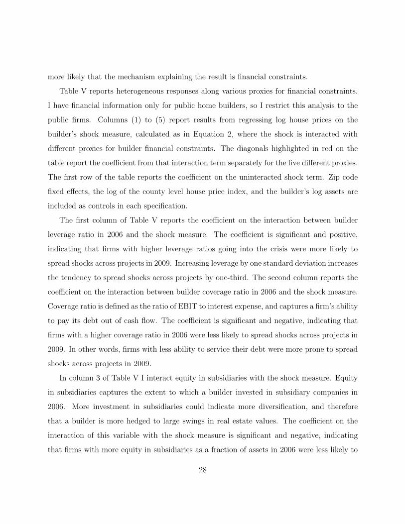
Table V reports heterogeneous responses along various proxies for financial constraints.

I have financial information only for public home builders, so I restrict this analysis to the

public firms. Columns (1) to (5) report results from regressing log house prices on the

builder’s shock measure, calculated as in Equation 2, where the shock is interacted with

different proxies for builder financial constraints. The diagonals highlighted in red on the

table report the coefficient from that interaction term separately for the five different proxies.

The first row of the table reports the coefficient on the uninteracted shock term. Zip code

fixed effects, the log of the county level house price index, and the builder’s log assets are

included as controls in each specification.

The first column of Table V reports the coefficient on the interaction between builder

leverage ratio in 2006 and the shock measure. The coefficient is significant and positive,

indicating that firms with higher leverage ratios going into the crisis were more likely to

spread shocks across projects in 2009. Increasing leverage by one standard deviation increases

the tendency to spread shocks across projects by one-third. The second column reports the

coefficient on the interaction between builder coverage ratio in 2006 and the shock measure.

Coverage ratio is defined as the ratio of EBIT to interest expense, and captures a firm’s ability

to pay its debt out of cash flow. The coefficient is significant and negative, indicating that

firms with a higher coverage ratio in 2006 were less likely to spread shocks across projects in

2009. In other words, firms with less ability to service their debt were more prone to spread

shocks across projects in 2009.

In column 3 of Table V I interact equity in subsidiaries with the shock measure. Equity

in subsidiaries captures the extent to which a builder invested in subsidiary companies in

2006. More investment in subsidiaries could indicate more diversification, and therefore

that a builder is more hedged to large swings in real estate values. The coefficient on the

interaction of this variable with the shock measure is significant and negative, indicating

that firms with more equity in subsidiaries as a fraction of assets in 2006 were less likely to

28

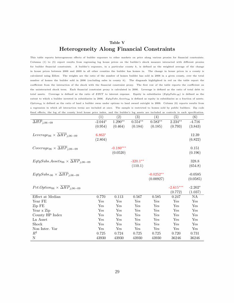
Table V

Heterogeneity Along Financial Constraints

This table reports heterogeneous effects of builder exposure to other markets on price along various proxies for financial constraints.

Columns (1) to (5) report results from regressing log house prices on the builder’s shock measure interacted with different proxies

for builder financial constraints. A builder’s exposure, in a particular county k, is defined as the weighted average of the change

in house prices between 2006 and 2009 in all other counties the builder has homes in. The change in house prices in a county is

calculated using Zillow. The weights are the ratio of the number of homes builder has sold in 2006 in a given county, over the total

number of homes the builder sold in 2006 (excluding sales in county k). The diagonals highlighted in red on the table report the

coefficient from the interaction of the shock with the financial constraint proxy. The first row of the table reports the coefficient on

the uninteracted shock term. Each financial constraint proxy is calculated in 2006. Leverage is defined as the ratio of total debt to

total assets. Coverage is defined as the ratio of EBIT to interest expense. Equity in subsidiaries (EqtySubs.06) is defined as the

extent to which a builder invested in subsidiaries in 2006. EqtySubs.Assets06 is defined as equity in subsidiaries as a fraction of assets.

Option06 is defined as the ratio of land a builder owns under options to land owned outright in 2006. Column (6) reports results from

a regression in which all interaction terms are included at once. The sample is restricted to homes sold by public builders. Zip code

fixed effects, the log of the county level house price index, and the builder’s log assets are included as controls in each specification.

(1) (2) (3) (4) (5) (6)

∆HP j,06−09 -2.044∗ 1.290∗∗ 0.554∗∗ 0.583∗∗ 2.234∗∗ -4.716(0.954) (0.464) (0.184) (0.185) (0.793) (3.843)

Leverage06 × ∆HP j,06−09 6.863∗ 12.39(2.804) (6.822)

Coverage06 × ∆HP j,06−09 -0.180∗∗∗ 0.151(0.0520) (0.196)

EqtySubs.Assets06 × ∆HP j,06−09 -320.1∗∗ 328.8(110.1) (654.8)

EqtySubs.06 × ∆HP j,06−09 -0.0252∗∗ -0.0585(0.00927) (0.0585)

Pct.Option06 × ∆HP j,06−09 -2.615∗∗∗ -2.202∗

(0.772) (1.037)Effect at Median 0.770 0.113 0.567 0.585 0.247 NAYear FE Yes Yes Yes Yes Yes YesZip FE Yes Yes Yes Yes Yes YesYear x Zip Yes Yes Yes Yes Yes YesCounty HP Index Yes Yes Yes Yes Yes YesLn Asset Yes Yes Yes Yes Yes YesShock Yes Yes Yes Yes Yes YesNon Inter. Var Yes Yes Yes Yes Yes YesR2 0.725 0.724 0.725 0.725 0.720 0.731N 43930 43930 43930 43930 36246 36246

29

spread shocks across projects in 2009. In other words, firms with possibly less diversification

going into the crisis were more prone to spread shocks across projects in 2009. The results

are similar when looking at equity in subsidiaries using levels rather than as a fraction of

assets.

I next use institutional details of the home building industry to construct a constraint

unique to builders. Column 5 reports the coefficient on the interaction between the ratio of

land a builder owned under options to land owned outright in 2006 and the shock measure.

Often, builders purchase land parcels using options, giving them the right to buy the land

outright at a certain price within a given date. When land values plummeted in 2009, builders

with more of their land owned via options rather than owned outright were in a stronger

financial position. The coefficient on the interaction of this variable with the shock measure is

significant and negative, indicating that firms more exposed to falling land values were more

prone to spread shocks across projects in 2009. Column 6 reports results from a regression

in which all interaction terms are included at once. Only Option06 remains significant, likely

because the multicollinearity of the proxies makes identifying separate effects difficult.

The first row of the bottom panel of Table V reports the effect of the shock calculated at

the median value of the financial constraint proxies. The effect of the shock at the median

value is positive for every measure used, indicating that in general, builders in this group

were spreading shocks across projects in 2009. For each proxy considered in Table V, builders

more likely to be financially constrained according to that proxy were more likely to spread

shocks across projects, evidence that the mechanism behind the effect is internal capital

markets.

The results in Table V exploit heterogeneity in financial constraints within the cross

section of public builders in 2009. However, there is also time series variation in financial

constraints within the builder industry as a whole. During the housing boom, credit stan-

dards were loose and builders could easily obtain loans, whereas the opposite was true during

the crisis. If the mechanism is internal capital markets, then in periods in which builders

30

could easily obtain loans, there should be no tendency for builders to spread shocks across

projects. Unconstrained builders will set listing times for their homes optimally, regardless

of whether they receive price shocks in distant projects. Because builders could easily obtain

financing during the boom period, there should be no effect.

To test this, I shift the main specification to the boom years, 2002 to 2005. In Equation

4, I regress the log sale price of house i, sold in month t in 2005, in county k, by builder j,

on builder j’s shock measure, which is calculated excluding house prices in county k.

Log(SalePricei,t,j,k,05) = β1∆HP j,02−05 + β2HPt,k + β3Xi + γs(i) + εi,t,j,k (4)

The shock measure is calculated as in Equation 2, but over years 2002 to 2005, as opposed to

over years 2006 to 2009 as in the main results. For brevity, in Equation 4, I denote the shock

measure during the boom,∑K

r 6=k ω02,r,j∆(HPr)02−05, as ∆HP j,02−05. Just like in Equation 2,

I include controls HPt,k for log county level house prices each month. All specifications also

include zip code fixed effects. Controls Xi include variables describing the characteristics

of house i, including: number of bathrooms, square footage, and property type (i.e., single

family home, condo, or duplex). Standard errors are clustered at the county level.

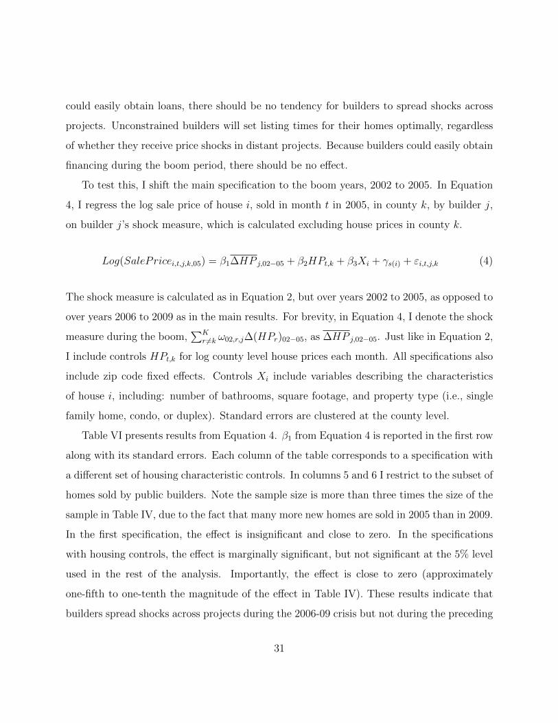
Table VI presents results from Equation 4. β1 from Equation 4 is reported in the first row

along with its standard errors. Each column of the table corresponds to a specification with

a different set of housing characteristic controls. In columns 5 and 6 I restrict to the subset of

homes sold by public builders. Note the sample size is more than three times the size of the

sample in Table IV, due to the fact that many more new homes are sold in 2005 than in 2009.

In the first specification, the effect is insignificant and close to zero. In the specifications

with housing controls, the effect is marginally significant, but not significant at the 5% level

used in the rest of the analysis. Importantly, the effect is close to zero (approximately

one-fifth to one-tenth the magnitude of the effect in Table IV). These results indicate that

builders spread shocks across projects during the 2006-09 crisis but not during the preceding

31

boom. Because builders were more likely to be financially unconstrained during the boom,

this finding is consistent with an internal capital markets mechanism. One threat to the

design is the possibility that builders learn from house price busts in crisis areas and use this

information to mark down prices in healthy regions in anticipation of the crisis spreading.

However, learning should occur during both booms and busts. Since I find linkages between

projects only during the crisis and not during the boom, learning cannot explain the results.

Table VI

House Prices and Builders’ Exposure to Other MarketsDuring the Boom

This table explores the effect of builders’ exposure to other housing markets on their pricing,measured at the housing transaction level during the boom period. The dependent variableis the log of house prices in 2005. The independent variable is the builder’s exposure to houseprice changes in distant counties in 2005. A builder’s exposure, in a particular county k, isdefined as the weighted average of the change in house prices between 2002 and 2005 in allother counties the builder has homes in. The change in house prices in a county is calculatedusing Zillow. The weights are the ratio of the number of homes builder has sold in 2002in a given county, over the total number of homes the builder sold in 2002 (excluding salesin county k). All regressions are ordinary least squares (OLS) and include zip code fixedeffects and log county house prices. Standard errors are clustered by county and are reportedin parentheses. ***, ** and * denote statistical significance at the .1%, 1% and 5% levels,respectively.

All Firms Public Only(1) (2) (3) (4) (5) (6)

∆HP j,02−05 -0.0501 -0.0424 -0.0419 -0.0424 0.113 -0.00473(0.0405) (0.0230) (0.0230) (0.0229) (0.128) (0.0628)

Zip FE Yes Yes Yes Yes Yes YesCounty HP Yes Yes Yes Yes Yes YesSq. Ft. No Yes Yes Yes No YesBaths No No Yes Yes No YesProp. Type FE No No No Yes No YesR2 0.687 0.833 0.833 0.835 0.773 0.886N 299847 299847 299847 299847 150926 150926

32

6.2 Effect on Listing Times

I find that builders respond to a loss in one project by cutting prices in unaffected projects.

For this result to imply that builders spread price shocks across projects via internal capital

markets, then it should be the case that when builders cut prices they sell homes faster. In

this section, I investigate whether builders experiencing negative shocks are more likely not

only to cut prices but also to sell their homes more quickly.25

I regress home listing times on the builder’s shock measure, calculated as in Equation 1,

using the same set of controls as in Equation 2. I estimate the regression on the sample of

homes that match to MLS, as described in Table III. Table VII reports coefficients on the

shock measure, β1, along with standard errors. The first five columns of the table refer to

specifications estimated over the full sample of builder home sales matched to MLS. The first

four columns use time-to-sale as the outcome variable and the fifth column uses sale price

as the outcome variable. The last two columns correspond to specifications restricted to the

sample of homes sold by public builders: columns 6 and 7 have time-to-sale and sale price

as outcome variables, respectively. All specifications include zip code by year fixed effects

and log county level monthly house prices. Interpreting the coefficient from column 4, I find

that builders exposed to a negative 10% shock, (roughly one standard deviation), sell homes

14 days more quickly.26 27 As I add controls to the specification using the full sample for

25A number of papers have shown that in general, cutting listing prices for homes results in faster timesto sale (Merlo et al., 2015; Genesove and Mayer, 1994; Levitt and Syverson, 2008). Guren (2018) shows thatthe effect of changing a home’s listing price on its time on the market is not linear in price. In particular,the relationship between price and time on the market is strongest when the home is above average price inan area. Builder home prices will almost always be above average price due to the new conditions of builderhomes, so this relationship should apply.

26To validate the result that constrained builders sell homes faster in the full sample of builder sales, inAppendix Section 11.3 I show that builders with exposure to housing bust markets are more likely to sell ahome in the same year it is built rather than in following years.

27I also validate my results against existing relationships between time-to-sale and price for resale homes.Guren (2018) finds that raising listing price of a home by 1% makes the home sell five to six days moreslowly. Interpreting the coefficient from Table IV, I find that builders with a negative shock of 4.6% cutprices by 1%. Using the listing times results in Table VII, I find that builders with a negative shock of 4.6%also sell homes 6 days more quickly, implying that when builders cut prices by 1% they sell homes 6 days

33

square footage, bathrooms, and property type, the coefficient remains stable in significance

and magnitude. Recall that the results from Table IV imply that builders exposed to a

negative 10% shock sell homes at a 2.2% discount. The coefficient in column 5 of Table

VII implies a similar result, that in the smaller sample of builder homes matched to listing

records, builders exposed to a negative 10% shock sell homes at a 2.1% discount.28 The

coefficient is not significant for the smaller, public only sample, which contains only 6,927

listings.

The results from columns 4 and 5 together indicate that builders trade off 2.1% in sale

price for selling 14 days sooner, implying an annualized discount rate of 72%. For comparison,

the average rate on builder debt is 14%29 during the boom period. Builders issued no debt

during the crisis. Builders likely only use internal financing from accelerated home sales when

external financing is excessively costly. If builders relied on an internal discount rate of 72%

in 2009, then the rate of external financing must have been greater than 72%, indicating that

the cost of external financing between the boom and the bust at the very least quadrupled

in size.

7 Heterogeneity

7.1 Time-to-Sale Sensitivity

The housing market features search frictions which produce a positive relationship between

price and time-to-sale. If builders are financially constrained and need cash quickly, they

faster. Assuming symmetric responses for raising and lowering listing price on time-to-sale, the relationshipI find is close to the one in Guren (2018).

28The above approach uses OLS to provide evidence that the duration until a home is sold is related to abuilder’s exposure to other markets. OLS assumes duration times are normally distributed; however, durationdata are often right skewed. I address the possibility that the normality assumption fails in Appendix Section11.2 by instead assuming that the homes’ duration times follow a Weibull distribution, which allows for fatright tails.

29Source: SDC Platinum.

34

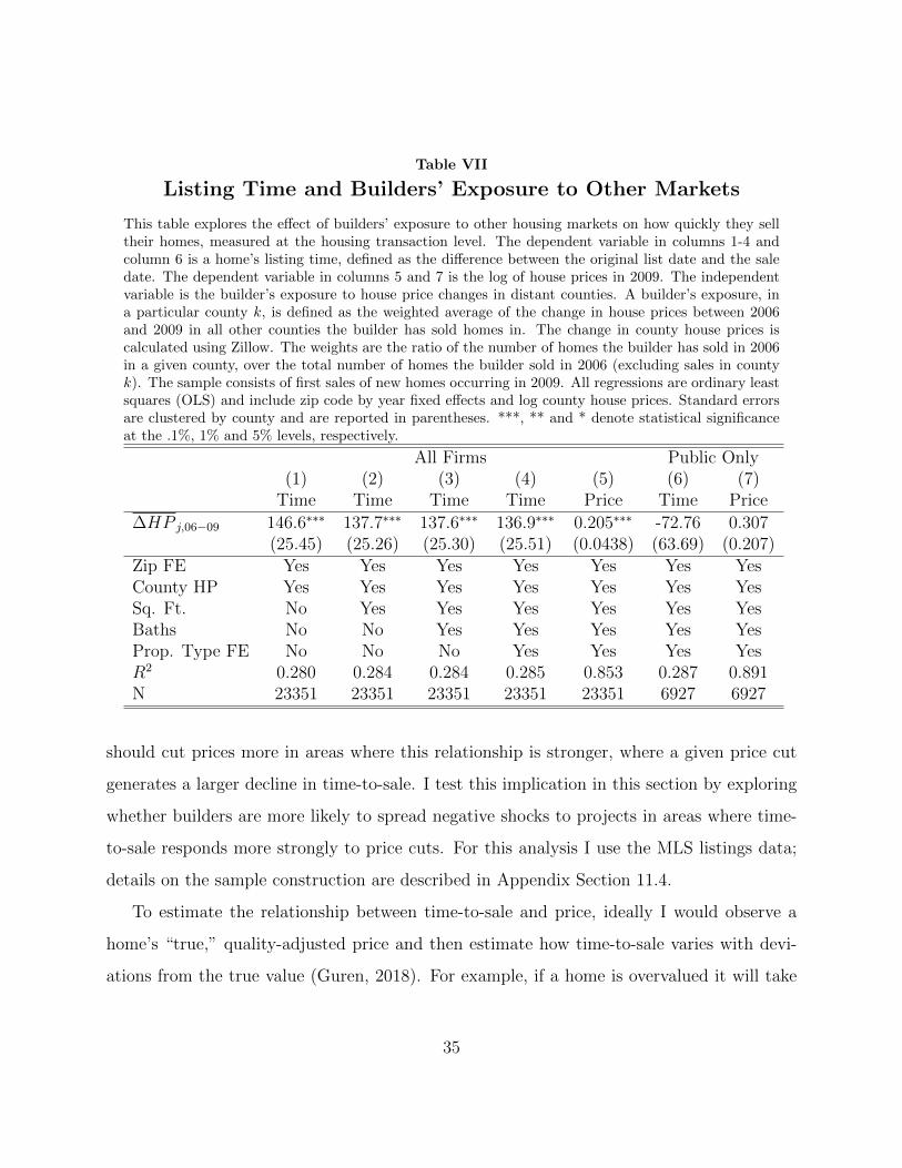
Table VII

Listing Time and Builders’ Exposure to Other Markets

This table explores the effect of builders’ exposure to other housing markets on how quickly they selltheir homes, measured at the housing transaction level. The dependent variable in columns 1-4 andcolumn 6 is a home’s listing time, defined as the difference between the original list date and the saledate. The dependent variable in columns 5 and 7 is the log of house prices in 2009. The independentvariable is the builder’s exposure to house price changes in distant counties. A builder’s exposure, ina particular county k, is defined as the weighted average of the change in house prices between 2006and 2009 in all other counties the builder has sold homes in. The change in county house prices iscalculated using Zillow. The weights are the ratio of the number of homes the builder has sold in 2006in a given county, over the total number of homes the builder sold in 2006 (excluding sales in countyk). The sample consists of first sales of new homes occurring in 2009. All regressions are ordinary leastsquares (OLS) and include zip code by year fixed effects and log county house prices. Standard errorsare clustered by county and are reported in parentheses. ***, ** and * denote statistical significanceat the .1%, 1% and 5% levels, respectively.

All Firms Public Only(1) (2) (3) (4) (5) (6) (7)

Time Time Time Time Price Time Price

∆HP j,06−09 146.6∗∗∗ 137.7∗∗∗ 137.6∗∗∗ 136.9∗∗∗ 0.205∗∗∗ -72.76 0.307(25.45) (25.26) (25.30) (25.51) (0.0438) (63.69) (0.207)

Zip FE Yes Yes Yes Yes Yes Yes YesCounty HP Yes Yes Yes Yes Yes Yes YesSq. Ft. No Yes Yes Yes Yes Yes YesBaths No No Yes Yes Yes Yes YesProp. Type FE No No No Yes Yes Yes YesR2 0.280 0.284 0.284 0.285 0.853 0.287 0.891N 23351 23351 23351 23351 23351 6927 6927

should cut prices more in areas where this relationship is stronger, where a given price cut

generates a larger decline in time-to-sale. I test this implication in this section by exploring

whether builders are more likely to spread negative shocks to projects in areas where time-

to-sale responds more strongly to price cuts. For this analysis I use the MLS listings data;

details on the sample construction are described in Appendix Section 11.4.

To estimate the relationship between time-to-sale and price, ideally I would observe a

home’s “true,” quality-adjusted price and then estimate how time-to-sale varies with devi-

ations from the true value (Guren, 2018). For example, if a home is overvalued it will take

35

longer to sell. In practice, we do not observe a home’s true value; instead I approximate

true value using a hedonic regression. To capture how time-to-sale changes with price, I

then estimate the relationship between the probability of sale within a given time and the

difference between realized price and predicted price (the mark-up).

To generate home i’s predicted price, pi,t, I regress log sale price, pi,t, on physical char-

acteristics, Xi, and date t and county k fixed effects, ξk,t, in Equation 5.

pi,t = βXi + ξk,t + εi,t (5)

I formalize the relationship between time-to-sale and price following Guren (2018), model-

ing the probability of a home selling within 13 weeks, di,t, as a function of predicted mark-up

and date and county fixed effects in Equation 6.

di,t = ρ (pi,t − pi,t)︸ ︷︷ ︸mark-up

+ξi,t + εi,t (6)

The mark-up is the residual from the hedonic regression in Equation 5. I estimate

Equation 6 grouping mark-up values into bins and I plot the coefficients on each mark-up

bin in Figure 7. Consistent with Guren (2018), the relationship between probability of sale

and mark-up in Figure 7 is concave and for positive mark-ups the relationship is negative.

When homes are overvalued, their probability of sale declines.

To identify regions where price cuts produce larger declines in time-to-sale, I generate

sensitivities of time-to-sale for each county.30 Next, I divide the main estimation sample into

quantiles according to the county time-to-sale elasticity to price and estimate Equation 2

within each quantile. I plot the coefficient on the builder shock measure from the regression

30I estimate Equation 6 within each county and define the county time-to-sale sensitivity as ρ ∗ (−1). Imultiply ρ by −1 for ease of interpretation.

36

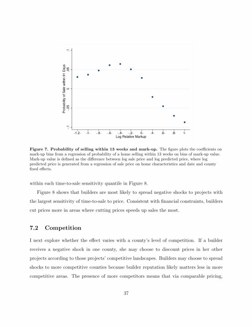
Figure 7. Probability of selling within 13 weeks and mark-up. The figure plots the coefficients onmark-up bins from a regression of probability of a home selling within 13 weeks on bins of mark-up value.Mark-up value is defined as the difference between log sale price and log predicted price, where logpredicted price is generated from a regression of sale price on home characteristics and date and countyfixed effects.

within each time-to-sale sensitivity quantile in Figure 8.

Figure 8 shows that builders are most likely to spread negative shocks to projects with

the largest sensitivity of time-to-sale to price. Consistent with financial constraints, builders

cut prices more in areas where cutting prices speeds up sales the most.

7.2 Competition

I next explore whether the effect varies with a county’s level of competition. If a builder

receives a negative shock in one county, she may choose to discount prices in her other

projects according to those projects’ competitive landscapes. Builders may choose to spread

shocks to more competitive counties because builder reputation likely matters less in more

competitive areas. The presence of more competitors means that via comparable pricing,

37

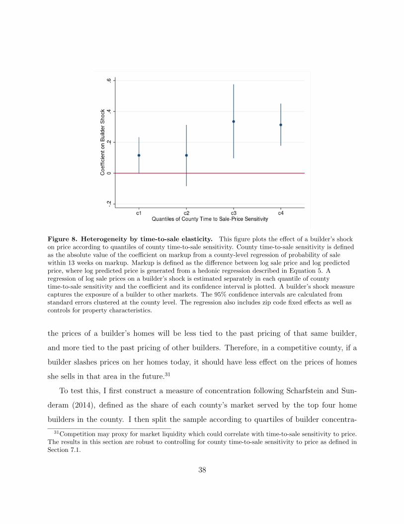
Figure 8. Heterogeneity by time-to-sale elasticity. This figure plots the effect of a builder’s shockon price according to quantiles of county time-to-sale sensitivity. County time-to-sale sensitivity is definedas the absolute value of the coefficient on markup from a county-level regression of probability of salewithin 13 weeks on markup. Markup is defined as the difference between log sale price and log predictedprice, where log predicted price is generated from a hedonic regression described in Equation 5. Aregression of log sale prices on a builder’s shock is estimated separately in each quantile of countytime-to-sale sensitivity and the coefficient and its confidence interval is plotted. A builder’s shock measurecaptures the exposure of a builder to other markets. The 95% confidence intervals are calculated fromstandard errors clustered at the county level. The regression also includes zip code fixed effects as well ascontrols for property characteristics.

the prices of a builder’s homes will be less tied to the past pricing of that same builder,

and more tied to the past pricing of other builders. Therefore, in a competitive county, if a

builder slashes prices on her homes today, it should have less effect on the prices of homes

she sells in that area in the future.31

To test this, I first construct a measure of concentration following Scharfstein and Sun-

deram (2014), defined as the share of each county’s market served by the top four home

builders in the county. I then split the sample according to quartiles of builder concentra-

31Competition may proxy for market liquidity which could correlate with time-to-sale sensitivity to price.The results in this section are robust to controlling for county time-to-sale sensitivity to price as defined inSection 7.1.

38

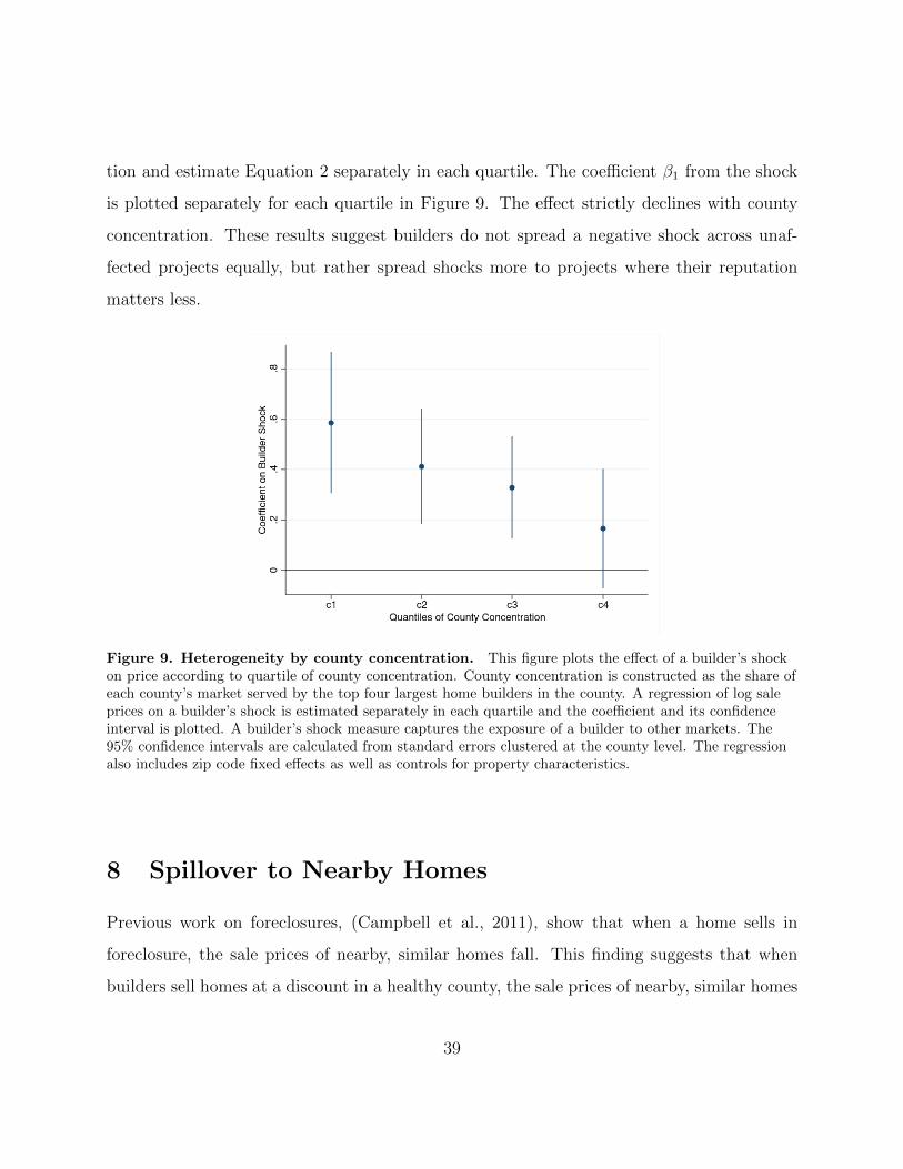
tion and estimate Equation 2 separately in each quartile. The coefficient β1 from the shock

is plotted separately for each quartile in Figure 9. The effect strictly declines with county

concentration. These results suggest builders do not spread a negative shock across unaf-

fected projects equally, but rather spread shocks more to projects where their reputation

matters less.

Figure 9. Heterogeneity by county concentration. This figure plots the effect of a builder’s shockon price according to quartile of county concentration. County concentration is constructed as the share ofeach county’s market served by the top four largest home builders in the county. A regression of log saleprices on a builder’s shock is estimated separately in each quartile and the coefficient and its confidenceinterval is plotted. A builder’s shock measure captures the exposure of a builder to other markets. The95% confidence intervals are calculated from standard errors clustered at the county level. The regressionalso includes zip code fixed effects as well as controls for property characteristics.

8 Spillover to Nearby Homes

Previous work on foreclosures, (Campbell et al., 2011), show that when a home sells in

foreclosure, the sale prices of nearby, similar homes fall. This finding suggests that when

builders sell homes at a discount in a healthy county, the sale prices of nearby, similar homes

39

may be affected. Declines in home prices are important; Mian and Sufi (2014) provide

evidence that declines in household net worth reduce consumer demand and employment.

Finding that in unaffected counties, a home sold at a discount by a constrained builder

causes nearby home prices to fall, suggests that builder internal networks are a channel of

geographic contagion.

I test for spillover pricing between builder and resale homes in this section. To identify

homes similar to builder ones, I restrict my sample to new homes, defined as those built after

2000. Recall I define a builder home sale as the first sale of a newly built home occurring

in 2009. To ensure I do not include any builder homes in this analysis of resale homes, I

require that the homes are first sold by a builder to a home-owner before 2008. I then restrict

my sample to sales of these homes occurring in 2009. A typical home in this group is first

sold from a builder to a home-owner in 2005, and then resold from the first home-owner

to another home-owner in 2009. These homes should be considered comparable to builder

homes, given their recent construction, but I will never count them as builder sales.

I next evaluate whether a shocked builder selling her home at a discount causes nearby

resale home prices to fall. I do this by testing if the sale price of a resale house is affected

by the shocks experienced by nearby builders. I define a resale home’s exposure to nearby

builder shocks as the weighted sum of the shocks experienced by builder homes sold in the

same zip code one month earlier. The weights in the sum are the inverse of the distance

between a resale house, i, and a builder house, j, referred to as distancei,j. Suppose a resale

home i is sold in zip code s in month t, and there are Jt−1 total builder homes sold in zip

code s in month t − 1. Then the aggregated shock for resale home i in zip code s, sold in

month t, is:

Aggr.Shocki,t,s,k,09 =

Jt−1∑j=1

1

distancei,j∗ shock∼k,j (7)

40

Where shock∼k,j is a builder’s shock,∑K

r 6=k ω06,r,j∆(HPr)06−09, or, ∆HP j,06−09, as defined

earlier in Equation 2. Intuitively, a shocked builder selling his house j at a discount in zip

code s, in month t − 1, will have a bigger effect on the sale price of house i in zip code s,

sold in month t, if the builder home j is closer to house i.

Equation 8 describes the main spillover specification.

LogSalePricei,t,s,k,09 = β1

Jt−1∑j=1

1

distancei,j∗ shock∼k,j + β2Xi+

HPt,k + γs(i) + δt + γs(i) ∗ δt + εi,t,s,k

(8)

I regress the log sale price of resale house i, sold in month t in 2009, in zip code s, in

county k, on home i’s exposure to nearby builder shocks, defined in Equation 7. I include

controls HPt,k for log county level house prices, as well as zip code fixed effects γs(i), and zip

code by year by month fixed effects, γs(i) ∗ δt. Controls Xi include variables describing the

characteristics of the house i.

Table VIII reports the results from Equation 8 in which the outcome variable is now

prices of resale homes. β1 is reported in the first row along with its standard errors. Each

column of the table corresponds to a specification with a different set of housing characteristic

controls. All specifications include zip code fixed effects and log county level monthly house

prices. Interpreting the coefficient from column 5, a home sale by a builder experiencing a

negative 10% shock causes the prices of resale homes within a 0.05 mi radius to fall by 1%.

To put this result in perspective, Campbell et al. (2011) find that a home sold in foreclosure

causes the prices of homes within a 0.05 mi radius to fall by 1%. When constrained builders

sell homes in healthy markets at a discount, nearby home prices fall. This result suggests

that builder internal capital markets serve as a channel of geographic contagion of negative

economic shocks.32

32Builder homes only make up a small fraction of total home sales in a county, so builders’ influence on

41

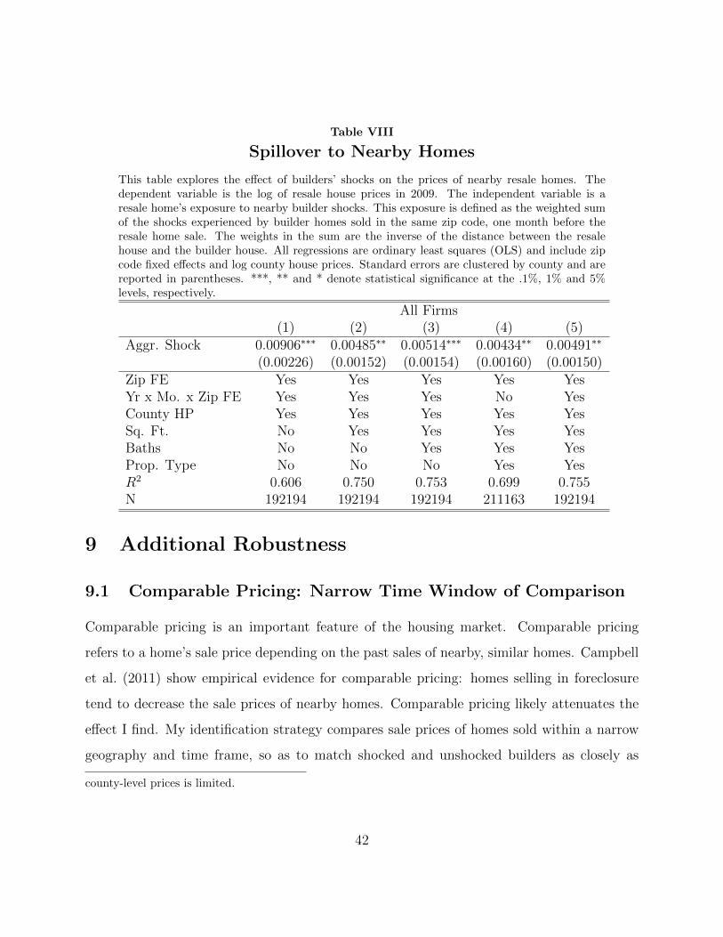
Table VIII

Spillover to Nearby Homes

This table explores the effect of builders’ shocks on the prices of nearby resale homes. Thedependent variable is the log of resale house prices in 2009. The independent variable is aresale home’s exposure to nearby builder shocks. This exposure is defined as the weighted sumof the shocks experienced by builder homes sold in the same zip code, one month before theresale home sale. The weights in the sum are the inverse of the distance between the resalehouse and the builder house. All regressions are ordinary least squares (OLS) and include zipcode fixed effects and log county house prices. Standard errors are clustered by county and arereported in parentheses. ***, ** and * denote statistical significance at the .1%, 1% and 5%levels, respectively.

All Firms(1) (2) (3) (4) (5)

Aggr. Shock 0.00906∗∗∗ 0.00485∗∗ 0.00514∗∗∗ 0.00434∗∗ 0.00491∗∗

(0.00226) (0.00152) (0.00154) (0.00160) (0.00150)Zip FE Yes Yes Yes Yes YesYr x Mo. x Zip FE Yes Yes Yes No YesCounty HP Yes Yes Yes Yes YesSq. Ft. No Yes Yes Yes YesBaths No No Yes Yes YesProp. Type No No No Yes YesR2 0.606 0.750 0.753 0.699 0.755N 192194 192194 192194 211163 192194

9 Additional Robustness

9.1 Comparable Pricing: Narrow Time Window of Comparison

Comparable pricing is an important feature of the housing market. Comparable pricing

refers to a home’s sale price depending on the past sales of nearby, similar homes. Campbell

et al. (2011) show empirical evidence for comparable pricing: homes selling in foreclosure

tend to decrease the sale prices of nearby homes. Comparable pricing likely attenuates the

effect I find. My identification strategy compares sale prices of homes sold within a narrow

geography and time frame, so as to match shocked and unshocked builders as closely as

county-level prices is limited.

42

possible. At the same time, homes sold within the same narrow geography and time frame

are also more likely to be priced off of each other. A shocked builder slashing prices on his

homes in one zip code will cause other builder homes in that same zip code to decline in

price. Comparable pricing of homes should therefore attenuate the effect.

To test that my effect would be stronger in the absence of comparable pricing, I narrow

the time fixed effects in Equation 2 from one year to one month. Comparable pricing is less

likely to have an effect in more narrow time frames because information on prices takes time

to disperse. In the extreme, if two homes sell on the same day, then neither home sale should

contaminate the price of the other.

Table IX reports results from adding zip code by year month fixed effects to Equation

2. β1 is reported in the first row along with its standard errors. Each column of the table

corresponds to a specification with a different set of housing characteristic controls. All

specifications include zip code by year month fixed effects and log county level monthly

house prices. The sample period corresponds to 2009, and the shock is calculated over 2006-

2009. Across every specification, the coefficient on β1 is larger than in the specifications

using only zip code by year fixed effects. This result suggests that comparable pricing likely

has attenuated the effect in Table IV.

9.2 Alternative Specifications

9.2.1 Additional Controls

The validity of my analysis rests on the assumption that shocked and unshocked builders do

not sell homes to different clienteles. If builders did sell to different socio-economic groups,

then there would be a difference in the luxury or quality of the homes builders sell. To test

the possibility that builders sell to different socio-economic groups, I add a host of additional

controls for housing quality to Equation 2, such as roof type, fireplace type, and condition

type. I do not include them in my main results in Table IV, because these variables are

43

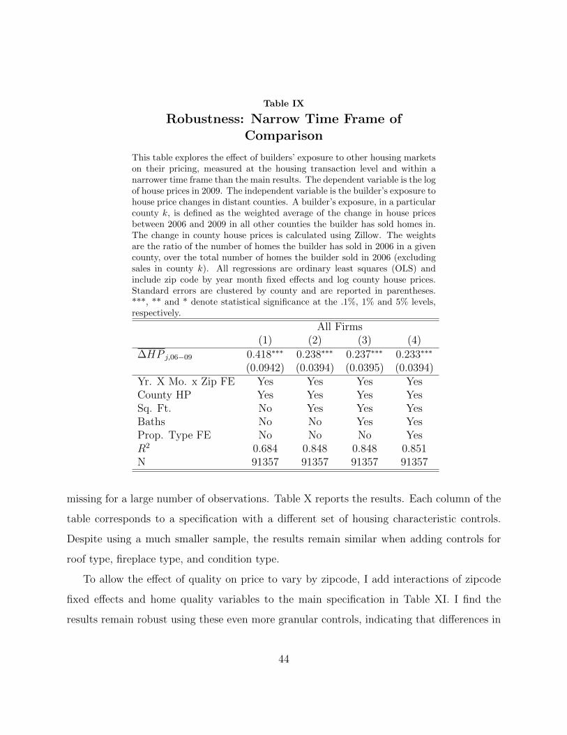
Table IX

Robustness: Narrow Time Frame ofComparison

This table explores the effect of builders’ exposure to other housing marketson their pricing, measured at the housing transaction level and within anarrower time frame than the main results. The dependent variable is the logof house prices in 2009. The independent variable is the builder’s exposure tohouse price changes in distant counties. A builder’s exposure, in a particularcounty k, is defined as the weighted average of the change in house pricesbetween 2006 and 2009 in all other counties the builder has sold homes in.The change in county house prices is calculated using Zillow. The weightsare the ratio of the number of homes the builder has sold in 2006 in a givencounty, over the total number of homes the builder sold in 2006 (excludingsales in county k). All regressions are ordinary least squares (OLS) andinclude zip code by year month fixed effects and log county house prices.Standard errors are clustered by county and are reported in parentheses.***, ** and * denote statistical significance at the .1%, 1% and 5% levels,respectively.

All Firms(1) (2) (3) (4)

∆HP j,06−09 0.418∗∗∗ 0.238∗∗∗ 0.237∗∗∗ 0.233∗∗∗

(0.0942) (0.0394) (0.0395) (0.0394)Yr. X Mo. x Zip FE Yes Yes Yes YesCounty HP Yes Yes Yes YesSq. Ft. No Yes Yes YesBaths No No Yes YesProp. Type FE No No No YesR2 0.684 0.848 0.848 0.851N 91357 91357 91357 91357

missing for a large number of observations. Table X reports the results. Each column of the

table corresponds to a specification with a different set of housing characteristic controls.

Despite using a much smaller sample, the results remain similar when adding controls for

roof type, fireplace type, and condition type.

To allow the effect of quality on price to vary by zipcode, I add interactions of zipcode

fixed effects and home quality variables to the main specification in Table XI. I find the

results remain robust using these even more granular controls, indicating that differences in

44

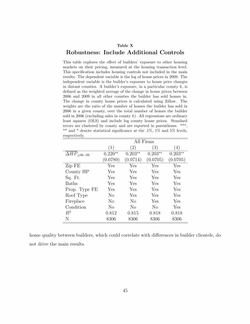
Table X

Robustness: Include Additional Controls

This table explores the effect of builders’ exposure to other housingmarkets on their pricing, measured at the housing transaction level.This specification includes housing controls not included in the mainresults. The dependent variable is the log of house prices in 2009. Theindependent variable is the builder’s exposure to house price changesin distant counties. A builder’s exposure, in a particular county k, isdefined as the weighted average of the change in house prices between2006 and 2009 in all other counties the builder has sold homes in.The change in county house prices is calculated using Zillow. Theweights are the ratio of the number of homes the builder has sold in2006 in a given county, over the total number of homes the buildersold in 2006 (excluding sales in county k). All regressions are ordinaryleast squares (OLS) and include log county house prices. Standarderrors are clustered by county and are reported in parentheses. ***,** and * denote statistical significance at the .1%, 1% and 5% levels,respectively.

All Firms(1) (2) (3) (4)

∆HP j,06−09 0.220∗∗ 0.203∗∗ 0.203∗∗ 0.203∗∗

(0.0789) (0.0714) (0.0705) (0.0705)Zip FE Yes Yes Yes YesCounty HP Yes Yes Yes YesSq. Ft. Yes Yes Yes YesBaths Yes Yes Yes YesProp. Type FE Yes Yes Yes YesRoof Type No Yes Yes YesFireplace No No Yes YesCondition No No No YesR2 0.812 0.815 0.818 0.818N 8306 8306 8306 8306

home quality between builders, which could correlate with differences in builder clientele, do

not drive the main results.

45

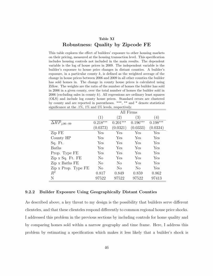
Table XI

Robustness: Quality by Zipcode FE

This table explores the effect of builders’ exposure to other housing marketson their pricing, measured at the housing transaction level. This specificationincludes housing controls not included in the main results. The dependentvariable is the log of house prices in 2009. The independent variable is thebuilder’s exposure to house price changes in distant counties. A builder’sexposure, in a particular county k, is defined as the weighted average of thechange in house prices between 2006 and 2009 in all other counties the builderhas sold homes in. The change in county house prices is calculated usingZillow. The weights are the ratio of the number of homes the builder has soldin 2006 in a given county, over the total number of homes the builder sold in2006 (excluding sales in county k). All regressions are ordinary least squares(OLS) and include log county house prices. Standard errors are clusteredby county and are reported in parentheses. ***, ** and * denote statisticalsignificance at the .1%, 1% and 5% levels, respectively.

All Firms(1) (2) (3) (4)

∆HP j,06−09 0.218∗∗∗ 0.201∗∗∗ 0.196∗∗∗ 0.198∗∗∗

(0.0373) (0.0321) (0.0333) (0.0334)Zip FE Yes Yes Yes YesCounty HP Yes Yes Yes YesSq. Ft. Yes Yes Yes YesBaths Yes Yes Yes YesProp. Type FE Yes Yes Yes YesZip x Sq. Ft. FE No Yes Yes YesZip x Baths FE No No Yes YesZip x Prop. Type FE No No No YesR2 0.817 0.849 0.859 0.862N 97522 97522 97522 97413

9.2.2 Builder Exposure Using Geographically Distant Counties

As described above, a key threat to my design is the possibility that builders serve different

clienteles, and that these clienteles respond differently to common regional house price shocks.

I addressed this problem in the previous sections by including controls for home quality and

by comparing homes sold within a narrow geography and time frame. Here, I address this

problem by estimating a specification which makes it less likely that a builder’s shock is

46

common to all regions. Specifically, I calculate a builder’s shock using only geographically

distant counties. I define a builder j’s county k-specific shock excluding house price changes

occurring in counties in the same state as county k. In Table XII I report results from

Equation 2, in which builder exposure to other markets has been modified to mean exposure

only to markets in other states. Each column of the table corresponds to a specification with

a different set of housing characteristic controls.

Table XII

Robustness: Geographically DistantCounties

This table explores the effect of builders’ exposure to very distant hous-ing markets on their pricing, measured at the housing transaction level.The dependent variable is the log of house prices in 2009. The inde-pendent variable is the builder’s exposure to house price changes indistant counties. A builder’s exposure, in a particular county k, is de-fined as the weighted average of the change in house prices between2006 and 2009 in all other counties the builder has sold homes in, ex-cluding counties in the same state as county k. The change in countyhouse prices is calculated using Zillow. The weights are the ratio of thenumber of homes the builder has sold in 2006 in a given county, overthe total number of homes the builder sold in 2006 (excluding salesin county k). All regressions are ordinary least squares (OLS) andinclude zip code fixed effects and log county house prices. Standarderrors are clustered by county and are reported in parentheses. ***,** and * denote statistical significance at the .1%, 1% and 5% levels,respectively.

All Firms(1) (2) (3) (4)

∆HP j,06−09 0.440∗∗∗ 0.211∗∗∗ 0.211∗∗∗ 0.206∗∗∗

(0.0825) (0.0398) (0.0398) (0.0406)Zip FE Yes Yes Yes YesCounty HP Yes Yes Yes YesSq. Ft. No Yes Yes YesBaths No No Yes YesProp. Type FE No No No YesR2 0.643 0.823 0.823 0.826N 84647 84647 84647 84647

47

This analysis will exclude builders operating in multiple counties within a single state,

and therefore the sample size falls. Nonetheless, the results remain similar to using this more

geographically distinct definition of a builder’s exposure to other regions. Interpreting the

coefficient from column 4, I find that a builder exposed to a 10% decline in house prices in

geographically distant markets cuts prices by 2.1%.

9.2.3 Resales of Distressed Builder Sales

If shocked builders sell to different socio-economic groups than non-shocked builders, then

there should be a difference in the quality of the homes these builders sell. In Table X I

test this possibility by controlling for a host of home quality characteristics, such as roof

type and foundation type, and find the results remain unchanged. Another way to test if

shocked builder homes have lower quality involves analyzing resales of builder homes. The

builder’s original financial condition should not affect the price of the home in the future.

Therefore, if a distressed builder home’s price is discounted due to the financial condition of

the builder, and not due to fundamentals of the home or its clientele, then the price of the

home will converge with time to the prices of non-distressed builder homes.

To investigate this idea, I test if the financial condition of the home’s builder, as captured

by the builder’s exposure to crisis areas, ∆HP j,06−09, predicts the home’s annualized rate of

return. Equation 9 reports this relationship. I regress the annualized return R of house i,

first sold by builder j in quarter t1 of 2009, and sold for a third time in quarter t3, in county k,

on builder j’s shock measure∑K

r 6=k ω06,r,j∆(HPr)06−09, which I denote as ∆HP j,06−09. Here

I include fixed effects ρi,t1,t3 for the quarter of the first sale interacted with the quarter of

the third sale. If a distressed builder home is not of lower quality than other builder homes,

then as the distressed builder home is sold in the future, its price should converge to other

home prices, resulting in a greater annualized return R and therefore a negative β1.

48

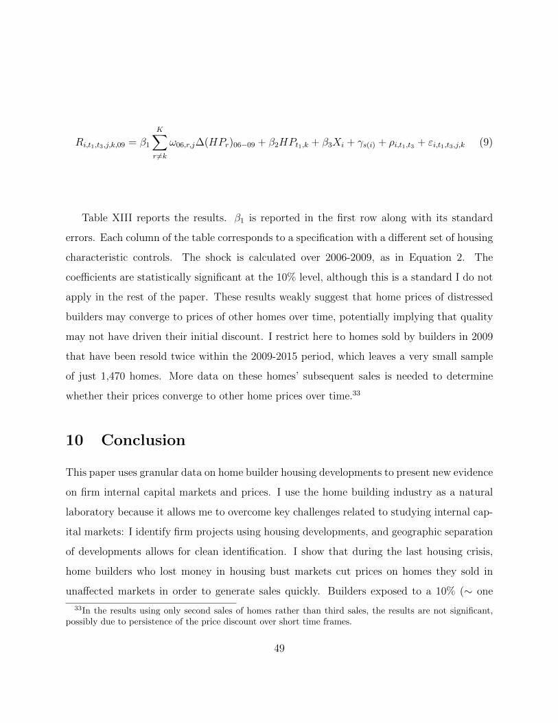
Ri,t1,t3,j,k,09 = β1

K∑r 6=k

ω06,r,j∆(HPr)06−09 + β2HPt1,k + β3Xi + γs(i) + ρi,t1,t3 + εi,t1,t3,j,k (9)

Table XIII reports the results. β1 is reported in the first row along with its standard

errors. Each column of the table corresponds to a specification with a different set of housing

characteristic controls. The shock is calculated over 2006-2009, as in Equation 2. The

coefficients are statistically significant at the 10% level, although this is a standard I do not

apply in the rest of the paper. These results weakly suggest that home prices of distressed

builders may converge to prices of other homes over time, potentially implying that quality

may not have driven their initial discount. I restrict here to homes sold by builders in 2009

that have been resold twice within the 2009-2015 period, which leaves a very small sample

of just 1,470 homes. More data on these homes’ subsequent sales is needed to determine

whether their prices converge to other home prices over time.33

10 Conclusion

This paper uses granular data on home builder housing developments to present new evidence

on firm internal capital markets and prices. I use the home building industry as a natural

laboratory because it allows me to overcome key challenges related to studying internal cap-

ital markets: I identify firm projects using housing developments, and geographic separation

of developments allows for clean identification. I show that during the last housing crisis,

home builders who lost money in housing bust markets cut prices on homes they sold in

unaffected markets in order to generate sales quickly. Builders exposed to a 10% (∼ one

33In the results using only second sales of homes rather than third sales, the results are not significant,possibly due to persistence of the price discount over short time frames.

49

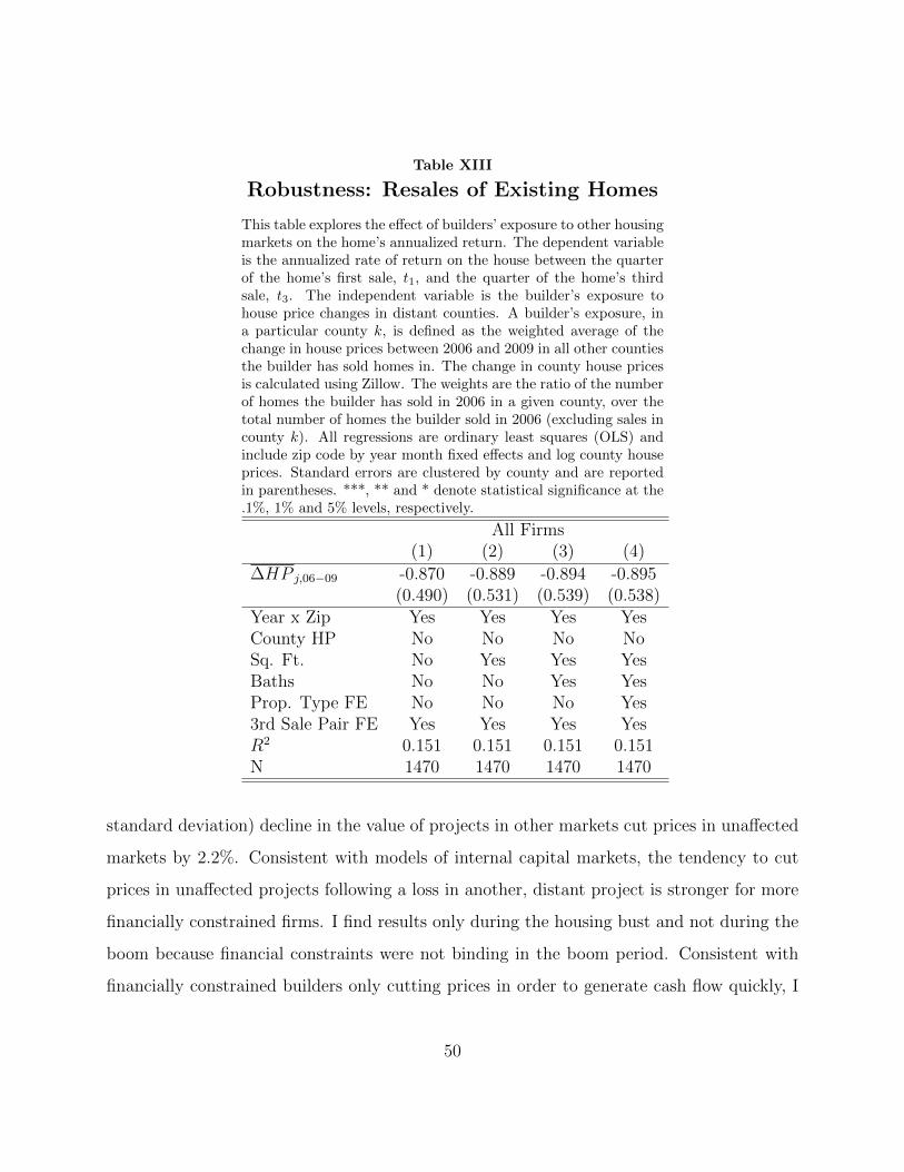
Table XIII

Robustness: Resales of Existing Homes

This table explores the effect of builders’ exposure to other housingmarkets on the home’s annualized return. The dependent variableis the annualized rate of return on the house between the quarterof the home’s first sale, t1, and the quarter of the home’s thirdsale, t3. The independent variable is the builder’s exposure tohouse price changes in distant counties. A builder’s exposure, ina particular county k, is defined as the weighted average of thechange in house prices between 2006 and 2009 in all other countiesthe builder has sold homes in. The change in county house pricesis calculated using Zillow. The weights are the ratio of the numberof homes the builder has sold in 2006 in a given county, over thetotal number of homes the builder sold in 2006 (excluding sales incounty k). All regressions are ordinary least squares (OLS) andinclude zip code by year month fixed effects and log county houseprices. Standard errors are clustered by county and are reportedin parentheses. ***, ** and * denote statistical significance at the.1%, 1% and 5% levels, respectively.

All Firms(1) (2) (3) (4)

∆HP j,06−09 -0.870 -0.889 -0.894 -0.895(0.490) (0.531) (0.539) (0.538)

Year x Zip Yes Yes Yes YesCounty HP No No No NoSq. Ft. No Yes Yes YesBaths No No Yes YesProp. Type FE No No No Yes3rd Sale Pair FE Yes Yes Yes YesR2 0.151 0.151 0.151 0.151N 1470 1470 1470 1470

standard deviation) decline in the value of projects in other markets cut prices in unaffected

markets by 2.2%. Consistent with models of internal capital markets, the tendency to cut

prices in unaffected projects following a loss in another, distant project is stronger for more

financially constrained firms. I find results only during the housing bust and not during the

boom because financial constraints were not binding in the boom period. Consistent with

financially constrained builders only cutting prices in order to generate cash flow quickly, I

50

show that when builders cut prices they sell homes faster and that builders are more likely

to spread price shocks to areas where price cuts lead to larger declines in time-to-sale.

This paper contributes to a large literature on the effects of financial frictions on economic

activity. When financial frictions force firms to rely on internal funds, shocks to one project

in a firm can affect unrelated projects. These spillovers matter because they imply that

financing constraints prevent firms from setting prices optimally. Moreover, they indicate

that negative economic shocks spread across geography via firm internal capital markets.

Bibliography

Alchian, A. A. Corporate management and property rights. Economic policy and the regu-

lation of corporate securities, 337:360, 1969.

Bailey, M., Cao, R., Kuchler, T., and Stroebel, J. The economic effects of social networks:

Evidence from the housing market. 2017.

Benmelech, E. and Bergman, N. K. Liquidation values and the credibility of financial contract

renegotiation: Evidence from us airlines. The Quarterly Journal of Economics, 123(4):

1635–1677, 2008.

Benmelech, E. and Bergman, N. K. Collateral pricing. Journal of financial Economics, 91

(3):339–360, 2009.

Benmelech, E. and Bergman, N. K. Bankruptcy and the collateral channel. The Journal of

Finance, 66(2):337–378, 2011.

Benmelech, E., Bergman, N., Milanez, A., and Mukharlyamov, V. The agglomeration of

bankruptcy. Technical report, National Bureau of Economic Research, 2014.

51

Berger, P. G. and Ofek, E. Diversification’s effect on firm value. Journal of financial eco-

nomics, 37(1):39–65, 1995.

Bernanke, B. and Gertler, M. Agency costs, net worth, and business fluctuation. American

Economic Review, 79(1):14–31, 1989.

Campbell, J. Y., Giglio, S., and Pathak, P. Forced sales and house prices. American

Economic Review, 101(5):2108–31, 2011.

Cetorelli, N. and Goldberg, L. S. Liquidity management of us global banks: Internal capital

markets in the great recession. Journal of International Economics, 88(2):299–311, 2012.

Chevalier, J. What do we know about cross-subsidization? evidence from merging firms.

Advances in Economic Analysis & Policy, 4(1), 2004.

Chevalier, J. A. Do lbo supermarkets charge more? an empirical analysis of the effects of

lbos on supermarket pricing. The Journal of Finance, 50(4):1095–1112, 1995.

Cortes, K. R. and Strahan, P. E. Tracing out capital flows: How financially integrated banks

respond to natural disasters. Journal of Financial Economics, 125(1):182–199, 2017.

Davis, M. A. and Heathcote, J. The price and quantity of residential land in the united

states. Journal of Monetary Economics, 54(8):2595–2620, 2007.

DeFusco, A., Ding, W., Ferreira, F., and Gyourko, J. The role of price spillovers in the

american housing boom. Journal of Urban Economics, 2018.

Ge, S. How do financial constraints affect product pricing? evidence from weather and life

insurance premiums. 2017.

Genesove, D. and Mayer, C. J. Equity and time to sale in the real estate market. Technical

report, National Bureau of Economic Research, 1994.

52

Gertner, R. H., Scharfstein, D. S., and Stein, J. C. Internal versus external capital markets.

The Quarterly Journal of Economics, 109(4):1211–1230, 1994.

Gilchrist, S., Schoenle, R., Sim, J., and Zakrajsek, E. Inflation dynamics during the financial

crisis. American Economic Review, 107(3):785–823, 2017.

Gilje, E. P., Loutskina, E., and Strahan, P. E. Exporting liquidity: Branch banking and

financial integration. The Journal of Finance, 71(3):1159–1184, 2016.

Giroud, X. and Mueller, H. M. Firms’ internal networks and local economic shocks. Technical

report, National Bureau of Economic Research, 2017.

Guren, A. M. House price momentum and strategic complementarity. Journal of Political

Economy, 126(3):1172–1218, 2018.

Haughwout, A., Peach, R. W., Sporn, J., and Tracy, J. The supply side of the housing boom

and bust of the 2000s. In Housing and the financial crisis, pages 69–104. University of

Chicago Press, 2012.

Kim, R. The effect of the credit crunch on output price dynamics: The corporate inventory

and liquidity management channel. 2018.

Kiyotaki, N. and Moore, J. Credit cycles. Journal of political economy, 105(2):211–248,

1997.

Lamont, O. Cash flow and investment: Evidence from internal capital markets. The Journal

of Finance, 52(1):83–109, 1997.

Lang, L. H. and Stulz, R. M. Tobin’s q, corporate diversification, and firm performance.

Journal of political economy, 102(6):1248–1280, 1994.

53

Levitt, S. D. and Syverson, C. Market distortions when agents are better informed: The

value of information in real estate transactions. The Review of Economics and Statistics,

90(4):599–611, 2008.

Merlo, A., Ortalo-Magne, F., and Rust, J. The home selling problem: Theory and evidence.

International Economic Review, 56(2):457–484, 2015.

Mian, A. and Sufi, A. What explains the 2007–2009 drop in employment? Econometrica,

82(6):2197–2223, 2014.

Mondragon, J. Household credit and employment in the great recession. Kilts Center for

Marketing at Chicago Booth–Nielsen Dataset Paper Series, pages 1–025, 2018.

Myers, S. C. and Majluf, N. S. Corporate financing and investment decisions when firms

have information that investors do not have. Journal of financial economics, 13(2):187–

221, 1984.

Nathanson, C. G. and Zwick, E. Arrested development: Theory and evidence of supply-

side speculation in the housing market. Technical report, National Bureau of Economic

Research, 2017.

Notowidigdo, M. J. The incidence of local labor demand shocks. Technical report, National

Bureau of Economic Research, 2011.

Ortiz-Molina, H. and Phillips, G. M. Asset liquidity and the cost of capital. Technical report,

National Bureau of Economic Research, 2010.

Peek, J. and Rosengren, E. S. Collateral damage: Effects of the japanese bank crisis on real

activity in the united states. American Economic Review, 90(1):30–45, 2000.

Pulvino, T. C. Do asset fire sales exist? an empirical investigation of commercial aircraft

transactions. The Journal of Finance, 53(3):939–978, 1998.

54

Rajan, R., Servaes, H., and Zingales, L. The cost of diversity: The diversification discount

and inefficient investment. The journal of Finance, 55(1):35–80, 2000.

Scharfstein, D. and Sunderam, A. Market power in mortgage lending and the transmission

of monetary policy. September, http://people. hbs. edu/asunderam/Mortgage, 20, 2014.

Scharfstein, D. S. and Stein, J. C. The dark side of internal capital markets: Divisional

rent-seeking and inefficient investment. The Journal of Finance, 55(6):2537–2564, 2000.

Shin, H.-H. and Park, Y. S. Financing constraints and internal capital markets: Evidence

from koreanchaebols’. Journal of corporate finance, 5(2):169–191, 1999.

Shleifer, A. and Vishny, R. Fire sales in finance and macroeconomics. Journal of Economic

Perspectives, 25(1):29–48, 2011.

Shleifer, A. and Vishny, R. W. Liquidation values and debt capacity: A market equilibrium

approach. The Journal of Finance, 47(4):1343–1366, 1992.

Stein, J. C. Internal capital markets and the competition for corporate resources. The

Journal of Finance, 52(1):111–133, 1997.

Whited, T. M. Is it inefficient investment that causes the diversification discount? The

Journal of Finance, 56(5):1667–1691, 2001.

Williamson, O. E. Markets and hierarchies. New York, 2630, 1975.

11 Appendix

11.1 Validate New Home Sales and Builder Assignment

I validate my measure of new home sales in this section by comparing new Census housing

permits to new home sales in my main estimation sample. First, I pull new housing permits

55

for only those counties which appear in Corelogic. The Census reports housing permits

according to category of home, in particular, 1, 2, 3, and 4+ unit dwellings. I focus on

single family, condominium, and duplex homes in Corelogic, so to match this definition

as closely as possible in the Census, I restrict to 1-3 unit dwellings.34 Reassuringly, the

correlation between my measure of new homes and Census new housing permits is 0.93.

Figure 10 plots the behavior of the two measures over time at the month level. Note that

the two measures should not be exactly the same because the Census reports housing starts,

whereas Corelogic reports finished home sales. As a result, we should expect a slight lag

between the two. Additionally, since there will be some housing constructions that are started

but never completed, the Census number of new housing starts may exceed the Corelogic

number of new homes sold. Overall, the two measures track each other closely, indicating

my identification of new homes is accurately picking up new house sales.

Next, I pull industry data to validate my classification of homes to builders. Recall

that I apply string matching methods to builder names from Corelogic transactions, and

group together homes according to these resulting company names. If my methods were not

adequate, then I should end up with market shares for builders that do not align with shares

reported in trade publications. To test this, I pull yearly rankings of builders from “Builder

Magazine,” an online trade report, in which rank is determined by number of homes sold.

I then rank builders in Corelogic in each year based on their number of homes sold. I plot

these two sets of rankings against each other in Figure 11. The plot comes close to fitting a

45 degree line, indicating that if a builder is ranked as number one in the trade publication

for selling the most homes that year, then I will also rank this builder as number one in

Corelogic for selling the most homes in that year. Over the full sample, approximately 60%

of firms listed in the trade publication appear in Corelogic.

34The 4+ unit dwelling Census category includes large condominiums which do not appear in my Corelogicsample.

56

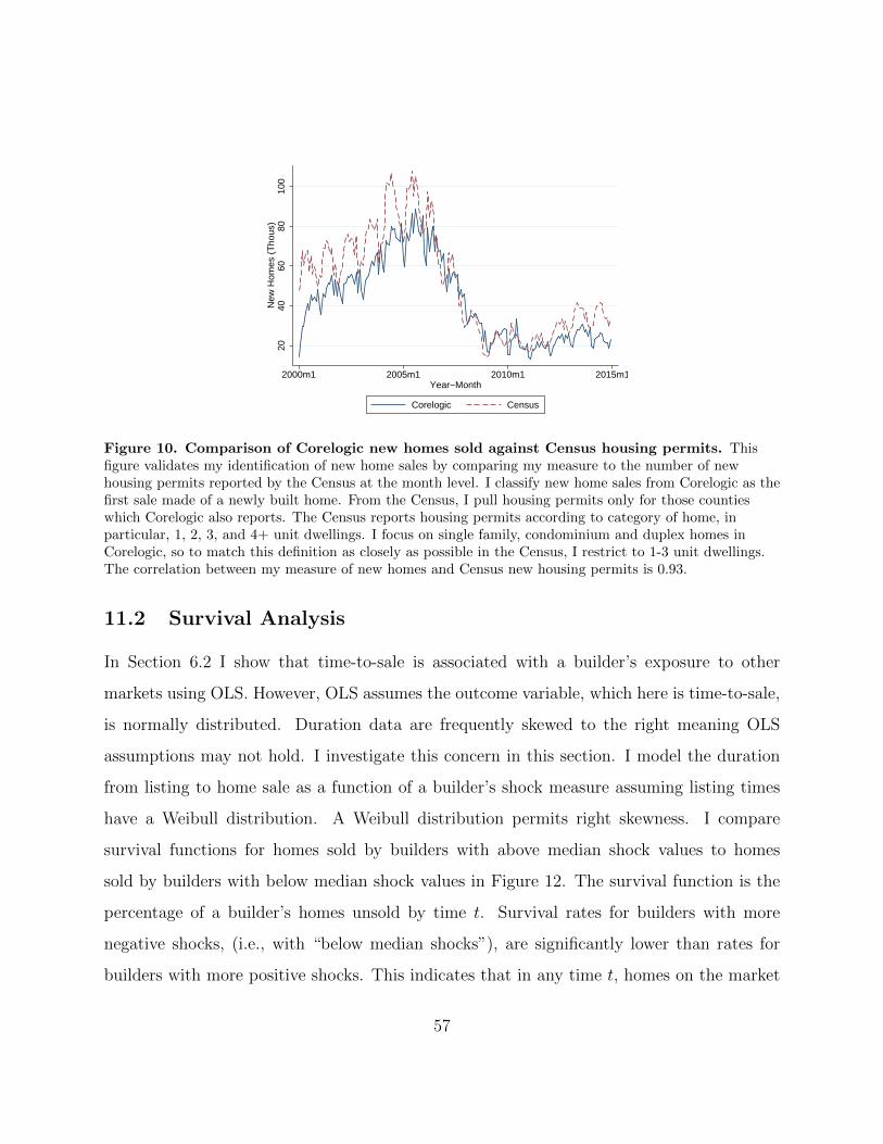
2040

6080

100

New

Hom

es (

Tho

us)

2000m1 2005m1 2010m1 2015m1Year−Month

Corelogic Census

Figure 10. Comparison of Corelogic new homes sold against Census housing permits. Thisfigure validates my identification of new home sales by comparing my measure to the number of newhousing permits reported by the Census at the month level. I classify new home sales from Corelogic as thefirst sale made of a newly built home. From the Census, I pull housing permits only for those countieswhich Corelogic also reports. The Census reports housing permits according to category of home, inparticular, 1, 2, 3, and 4+ unit dwellings. I focus on single family, condominium and duplex homes inCorelogic, so to match this definition as closely as possible in the Census, I restrict to 1-3 unit dwellings.The correlation between my measure of new homes and Census new housing permits is 0.93.

11.2 Survival Analysis

In Section 6.2 I show that time-to-sale is associated with a builder’s exposure to other

markets using OLS. However, OLS assumes the outcome variable, which here is time-to-sale,

is normally distributed. Duration data are frequently skewed to the right meaning OLS

assumptions may not hold. I investigate this concern in this section. I model the duration

from listing to home sale as a function of a builder’s shock measure assuming listing times

have a Weibull distribution. A Weibull distribution permits right skewness. I compare

survival functions for homes sold by builders with above median shock values to homes

sold by builders with below median shock values in Figure 12. The survival function is the

percentage of a builder’s homes unsold by time t. Survival rates for builders with more

negative shocks, (i.e., with “below median shocks”), are significantly lower than rates for

builders with more positive shocks. This indicates that in any time t, homes on the market

57

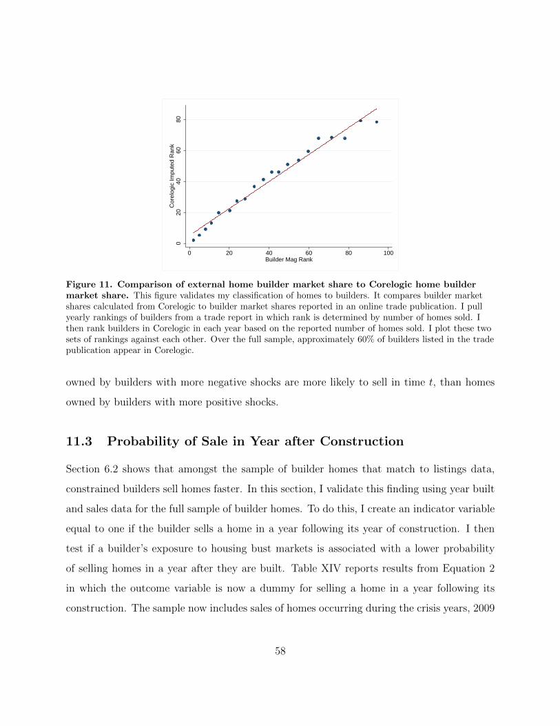
020

4060

80C

orel

ogic

Impu

ted

Ran

k

0 20 40 60 80 100Builder Mag Rank

Figure 11. Comparison of external home builder market share to Corelogic home buildermarket share. This figure validates my classification of homes to builders. It compares builder marketshares calculated from Corelogic to builder market shares reported in an online trade publication. I pullyearly rankings of builders from a trade report in which rank is determined by number of homes sold. Ithen rank builders in Corelogic in each year based on the reported number of homes sold. I plot these twosets of rankings against each other. Over the full sample, approximately 60% of builders listed in the tradepublication appear in Corelogic.

owned by builders with more negative shocks are more likely to sell in time t, than homes

owned by builders with more positive shocks.

11.3 Probability of Sale in Year after Construction

Section 6.2 shows that amongst the sample of builder homes that match to listings data,

constrained builders sell homes faster. In this section, I validate this finding using year built

and sales data for the full sample of builder homes. To do this, I create an indicator variable

equal to one if the builder sells a home in a year following its year of construction. I then

test if a builder’s exposure to housing bust markets is associated with a lower probability

of selling homes in a year after they are built. Table XIV reports results from Equation 2

in which the outcome variable is now a dummy for selling a home in a year following its

construction. The sample now includes sales of homes occurring during the crisis years, 2009

58

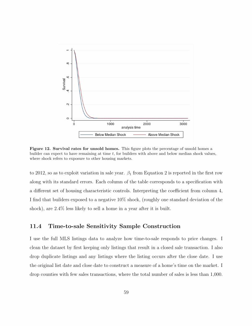
Figure 12. Survival rates for unsold homes. This figure plots the percentage of unsold homes abuilder can expect to have remaining at time t, for builders with above and below median shock values,where shock refers to exposure to other housing markets.

to 2012, so as to exploit variation in sale year. β1 from Equation 2 is reported in the first row

along with its standard errors. Each column of the table corresponds to a specification with

a different set of housing characteristic controls. Interpreting the coefficient from column 4,

I find that builders exposed to a negative 10% shock, (roughly one standard deviation of the

shock), are 2.4% less likely to sell a home in a year after it is built.

11.4 Time-to-sale Sensitivity Sample Construction

I use the full MLS listings data to analyze how time-to-sale responds to price changes. I

clean the dataset by first keeping only listings that result in a closed sale transaction. I also

drop duplicate listings and any listings where the listing occurs after the close date. I use

the original list date and close date to construct a measure of a home’s time on the market. I

drop counties with few sales transactions, where the total number of sales is less than 1,000.

59

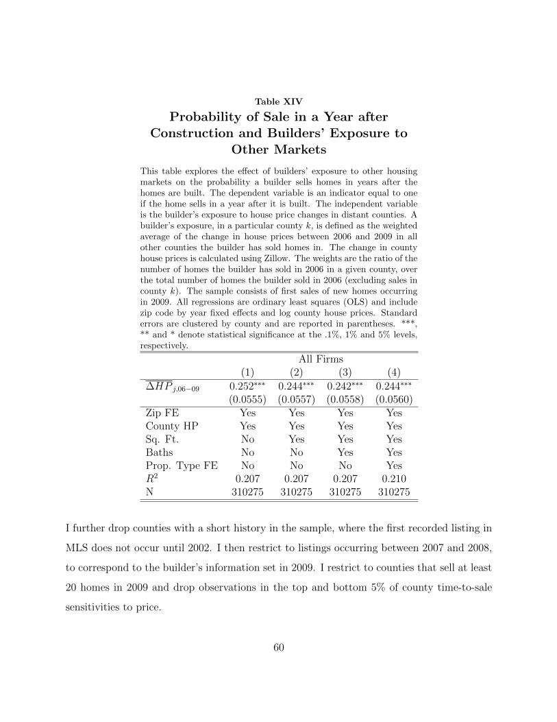
Table XIV

Probability of Sale in a Year afterConstruction and Builders’ Exposure to

Other Markets

This table explores the effect of builders’ exposure to other housingmarkets on the probability a builder sells homes in years after thehomes are built. The dependent variable is an indicator equal to oneif the home sells in a year after it is built. The independent variableis the builder’s exposure to house price changes in distant counties. Abuilder’s exposure, in a particular county k, is defined as the weightedaverage of the change in house prices between 2006 and 2009 in allother counties the builder has sold homes in. The change in countyhouse prices is calculated using Zillow. The weights are the ratio of thenumber of homes the builder has sold in 2006 in a given county, overthe total number of homes the builder sold in 2006 (excluding sales incounty k). The sample consists of first sales of new homes occurringin 2009. All regressions are ordinary least squares (OLS) and includezip code by year fixed effects and log county house prices. Standarderrors are clustered by county and are reported in parentheses. ***,** and * denote statistical significance at the .1%, 1% and 5% levels,respectively.

All Firms(1) (2) (3) (4)

∆HP j,06−09 0.252∗∗∗ 0.244∗∗∗ 0.242∗∗∗ 0.244∗∗∗

(0.0555) (0.0557) (0.0558) (0.0560)Zip FE Yes Yes Yes YesCounty HP Yes Yes Yes YesSq. Ft. No Yes Yes YesBaths No No Yes YesProp. Type FE No No No YesR2 0.207 0.207 0.207 0.210N 310275 310275 310275 310275

I further drop counties with a short history in the sample, where the first recorded listing in

MLS does not occur until 2002. I then restrict to listings occurring between 2007 and 2008,

to correspond to the builder’s information set in 2009. I restrict to counties that sell at least

20 homes in 2009 and drop observations in the top and bottom 5% of county time-to-sale

sensitivities to price.

60

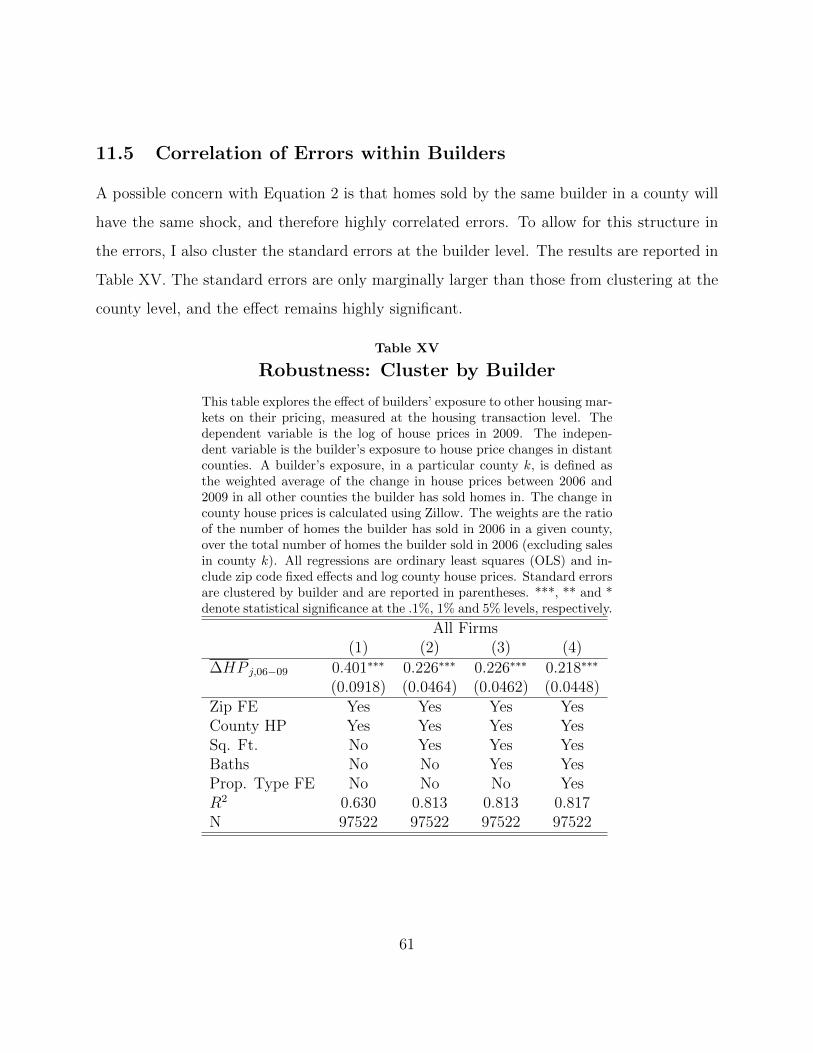
11.5 Correlation of Errors within Builders

A possible concern with Equation 2 is that homes sold by the same builder in a county will

have the same shock, and therefore highly correlated errors. To allow for this structure in

the errors, I also cluster the standard errors at the builder level. The results are reported in

Table XV. The standard errors are only marginally larger than those from clustering at the

county level, and the effect remains highly significant.

Table XV

Robustness: Cluster by Builder

This table explores the effect of builders’ exposure to other housing mar-kets on their pricing, measured at the housing transaction level. Thedependent variable is the log of house prices in 2009. The indepen-dent variable is the builder’s exposure to house price changes in distantcounties. A builder’s exposure, in a particular county k, is defined asthe weighted average of the change in house prices between 2006 and2009 in all other counties the builder has sold homes in. The change incounty house prices is calculated using Zillow. The weights are the ratioof the number of homes the builder has sold in 2006 in a given county,over the total number of homes the builder sold in 2006 (excluding salesin county k). All regressions are ordinary least squares (OLS) and in-clude zip code fixed effects and log county house prices. Standard errorsare clustered by builder and are reported in parentheses. ***, ** and *denote statistical significance at the .1%, 1% and 5% levels, respectively.

All Firms(1) (2) (3) (4)

∆HP j,06−09 0.401∗∗∗ 0.226∗∗∗ 0.226∗∗∗ 0.218∗∗∗

(0.0918) (0.0464) (0.0462) (0.0448)Zip FE Yes Yes Yes YesCounty HP Yes Yes Yes YesSq. Ft. No Yes Yes YesBaths No No Yes YesProp. Type FE No No No YesR2 0.630 0.813 0.813 0.817N 97522 97522 97522 97522

61

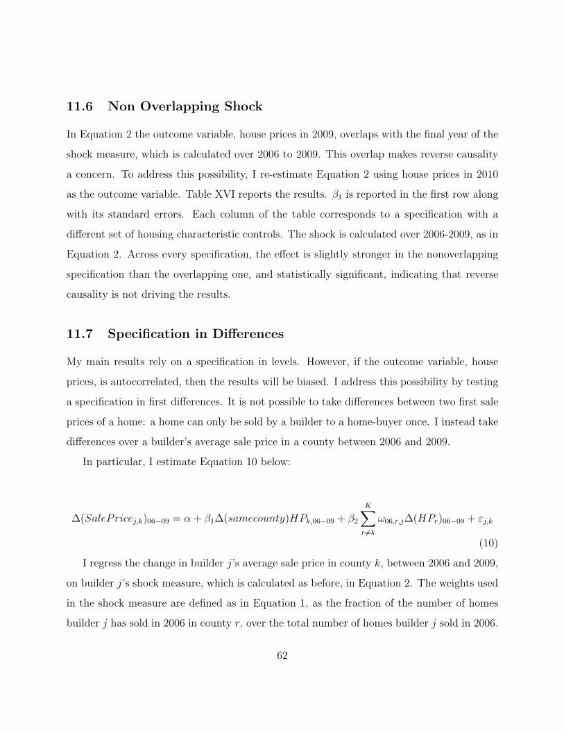
11.6 Non Overlapping Shock

In Equation 2 the outcome variable, house prices in 2009, overlaps with the final year of the

shock measure, which is calculated over 2006 to 2009. This overlap makes reverse causality

a concern. To address this possibility, I re-estimate Equation 2 using house prices in 2010

as the outcome variable. Table XVI reports the results. β1 is reported in the first row along

with its standard errors. Each column of the table corresponds to a specification with a

different set of housing characteristic controls. The shock is calculated over 2006-2009, as in

Equation 2. Across every specification, the effect is slightly stronger in the nonoverlapping

specification than the overlapping one, and statistically significant, indicating that reverse

causality is not driving the results.

11.7 Specification in Differences

My main results rely on a specification in levels. However, if the outcome variable, house

prices, is autocorrelated, then the results will be biased. I address this possibility by testing

a specification in first differences. It is not possible to take differences between two first sale

prices of a home: a home can only be sold by a builder to a home-buyer once. I instead take

differences over a builder’s average sale price in a county between 2006 and 2009.

In particular, I estimate Equation 10 below:

∆(SalePricej,k)06−09 = α + β1∆(samecounty)HPk,06−09 + β2

K∑r 6=k

ω06,r,j∆(HPr)06−09 + εj,k

(10)

I regress the change in builder j’s average sale price in county k, between 2006 and 2009,

on builder j’s shock measure, which is calculated as before, in Equation 2. The weights used

in the shock measure are defined as in Equation 1, as the fraction of the number of homes

builder j has sold in 2006 in county r, over the total number of homes builder j sold in 2006.

62

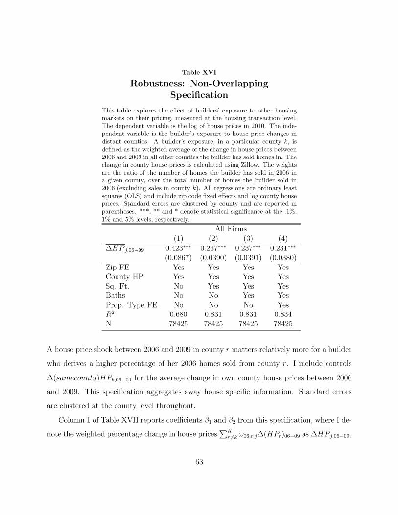
Table XVI

Robustness: Non-OverlappingSpecification

This table explores the effect of builders’ exposure to other housingmarkets on their pricing, measured at the housing transaction level.The dependent variable is the log of house prices in 2010. The inde-pendent variable is the builder’s exposure to house price changes indistant counties. A builder’s exposure, in a particular county k, isdefined as the weighted average of the change in house prices between2006 and 2009 in all other counties the builder has sold homes in. Thechange in county house prices is calculated using Zillow. The weightsare the ratio of the number of homes the builder has sold in 2006 ina given county, over the total number of homes the builder sold in2006 (excluding sales in county k). All regressions are ordinary leastsquares (OLS) and include zip code fixed effects and log county houseprices. Standard errors are clustered by county and are reported inparentheses. ***, ** and * denote statistical significance at the .1%,1% and 5% levels, respectively.

All Firms(1) (2) (3) (4)

∆HP j,06−09 0.423∗∗∗ 0.237∗∗∗ 0.237∗∗∗ 0.231∗∗∗

(0.0867) (0.0390) (0.0391) (0.0380)Zip FE Yes Yes Yes YesCounty HP Yes Yes Yes YesSq. Ft. No Yes Yes YesBaths No No Yes YesProp. Type FE No No No YesR2 0.680 0.831 0.831 0.834N 78425 78425 78425 78425

A house price shock between 2006 and 2009 in county r matters relatively more for a builder

who derives a higher percentage of her 2006 homes sold from county r. I include controls

∆(samecounty)HPk,06−09 for the average change in own county house prices between 2006

and 2009. This specification aggregates away house specific information. Standard errors

are clustered at the county level throughout.

Column 1 of Table XVII reports coefficients β1 and β2 from this specification, where I de-

note the weighted percentage change in house prices∑K

r 6=k ω06,r,j∆(HPr)06−09 as ∆HP j,06−09,

63

as before. The positive sign and statistical significance of the coefficient on ∆HP j,06−09 in-

dicates that builders spread price shocks to unaffected counties. Reassuringly, these results

indicate that the effect found in Table IV is not driven by autocorrelation in house prices.

I next test for an effect during the boom using the same specification. Column 2 of Table

XVII reports coefficients β1 and β2 from Equation 10 that has now been shifted back to the

boom period, 2002 to 2005. The coefficient on ∆HP j,02−05 is statistically insignificant and

much smaller in magnitude than the effect during the crisis. Thus, using specifications in

levels and in differences, I find that builders spread shocks only during the crisis and not

during the boom.

11.8 Additional Robustness

64

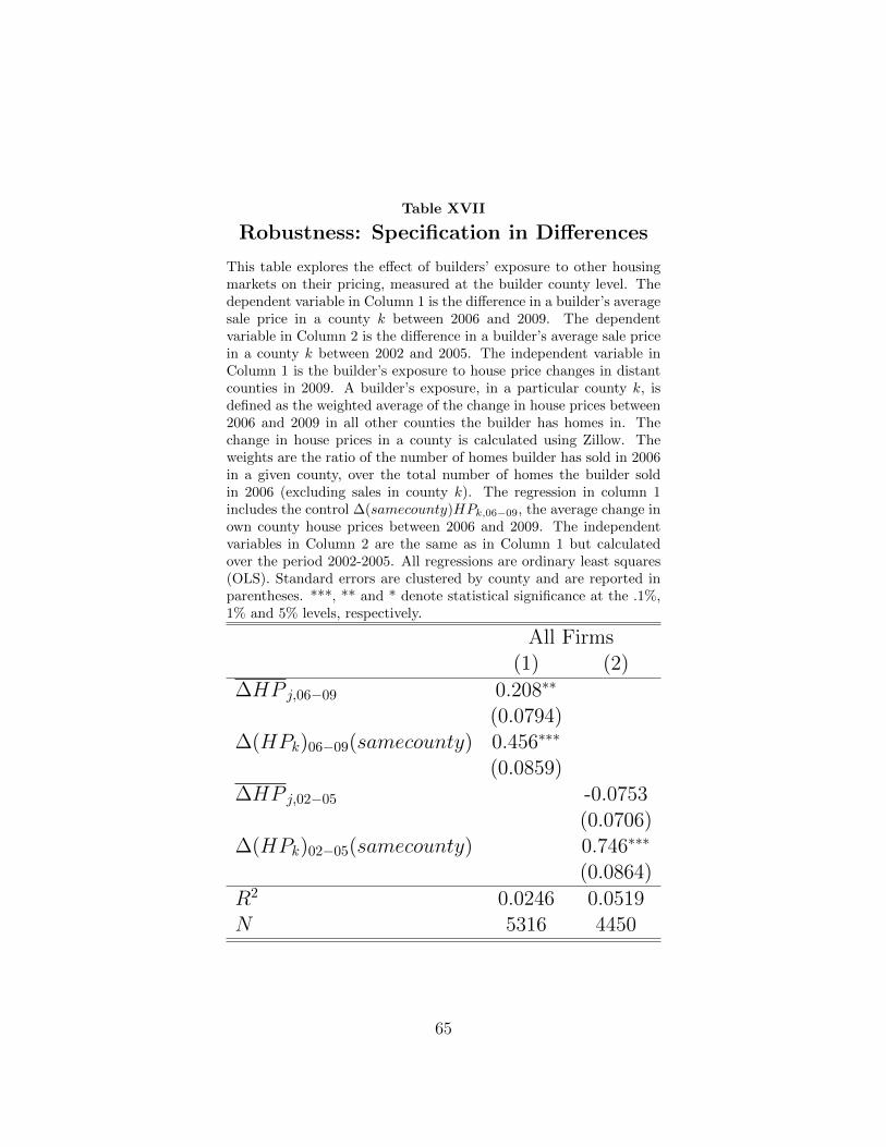
Table XVII

Robustness: Specification in Differences

This table explores the effect of builders’ exposure to other housingmarkets on their pricing, measured at the builder county level. Thedependent variable in Column 1 is the difference in a builder’s averagesale price in a county k between 2006 and 2009. The dependentvariable in Column 2 is the difference in a builder’s average sale pricein a county k between 2002 and 2005. The independent variable inColumn 1 is the builder’s exposure to house price changes in distantcounties in 2009. A builder’s exposure, in a particular county k, isdefined as the weighted average of the change in house prices between2006 and 2009 in all other counties the builder has homes in. Thechange in house prices in a county is calculated using Zillow. Theweights are the ratio of the number of homes builder has sold in 2006in a given county, over the total number of homes the builder soldin 2006 (excluding sales in county k). The regression in column 1includes the control ∆(samecounty)HPk,06−09, the average change inown county house prices between 2006 and 2009. The independentvariables in Column 2 are the same as in Column 1 but calculatedover the period 2002-2005. All regressions are ordinary least squares(OLS). Standard errors are clustered by county and are reported inparentheses. ***, ** and * denote statistical significance at the .1%,1% and 5% levels, respectively.

All Firms(1) (2)

∆HP j,06−09 0.208∗∗

(0.0794)∆(HPk)06−09(samecounty) 0.456∗∗∗

(0.0859)

∆HP j,02−05 -0.0753(0.0706)

∆(HPk)02−05(samecounty) 0.746∗∗∗

(0.0864)

R2 0.0246 0.0519N 5316 4450

65

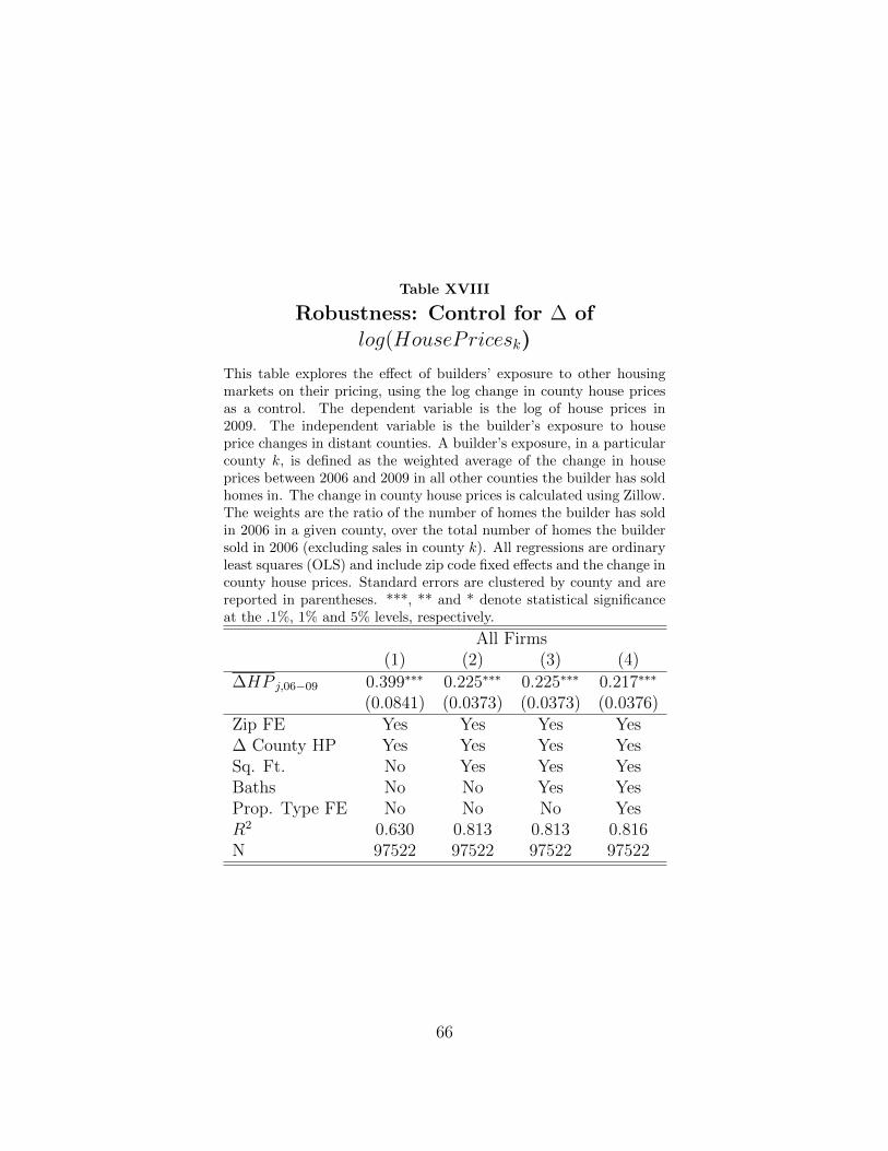
Table XVIII

Robustness: Control for ∆ oflog(HousePricesk)

This table explores the effect of builders’ exposure to other housingmarkets on their pricing, using the log change in county house pricesas a control. The dependent variable is the log of house prices in2009. The independent variable is the builder’s exposure to houseprice changes in distant counties. A builder’s exposure, in a particularcounty k, is defined as the weighted average of the change in houseprices between 2006 and 2009 in all other counties the builder has soldhomes in. The change in county house prices is calculated using Zillow.The weights are the ratio of the number of homes the builder has soldin 2006 in a given county, over the total number of homes the buildersold in 2006 (excluding sales in county k). All regressions are ordinaryleast squares (OLS) and include zip code fixed effects and the change incounty house prices. Standard errors are clustered by county and arereported in parentheses. ***, ** and * denote statistical significanceat the .1%, 1% and 5% levels, respectively.

All Firms(1) (2) (3) (4)

∆HP j,06−09 0.399∗∗∗ 0.225∗∗∗ 0.225∗∗∗ 0.217∗∗∗

(0.0841) (0.0373) (0.0373) (0.0376)Zip FE Yes Yes Yes Yes∆ County HP Yes Yes Yes YesSq. Ft. No Yes Yes YesBaths No No Yes YesProp. Type FE No No No YesR2 0.630 0.813 0.813 0.816N 97522 97522 97522 97522

66

Table XIX

Robustness: Exposure at Zip Code Level

This table explores the effect of builders’ exposure to other housingmarkets on their pricing, calculated at the zip code level. The de-pendent variable is the log of house prices in 2009. The independentvariable is the builder’s exposure to house price changes in distant zipcodes. A builder’s exposure, in a particular zip code k, is defined asthe weighted average of the change in house prices between 2006 and2009 in all other zip codes the builder has sold homes in. The changein zip code house prices is calculated using Zillow. The weights are theratio of the number of homes the builder has sold in 2006 in a givenzip code, over the total number of homes the builder sold in 2006 (ex-cluding sales in zip code k). All regressions are ordinary least squares(OLS) and include zip code fixed effects. Standard errors are clus-tered by county and are reported in parentheses. ***, ** and * denotestatistical significance at the .1%, 1% and 5% levels, respectively.

All Firms(1) (2) (3) (4)

∆HP j,06−09 0.405∗∗∗ 0.222∗∗∗ 0.222∗∗∗ 0.220∗∗∗

(0.0758) (0.0375) (0.0375) (0.0388)Zip FE Yes Yes Yes YesZip HP Yes Yes Yes YesSq. Ft. No Yes Yes YesBaths No No Yes YesProp. Type FE No No No YesR2 0.622 0.802 0.802 0.804N 81345 81345 81345 81345

67