Embed Size (px)
Citation preview

1
Designing Stated Choice Experiments:
State-of-the-ArtMichiel Bliemer
The University of Sydney, AustraliaInstitute of Transport & Logistics Studies
Delft University of Technology, The NetherlandsDepartment of Transport & Planning
John Rose
The University of Sydney, AustraliaInstitute of Transport & Logistics Studies
ETH Zurich
5th December 2007

2
Contents
• Stated choice experiments• Creating stated choice experiments• Generating experimental designs
o Full factorial designso Orthogonal designso Efficient designso Other designs (constrained, pivot, covariates)
• How to generate designs?

3
What are Stated Choice experiments?
Paper and Pencil Surveys
CAPI Surveys
Internet Surveys

4
What are Stated Choice experiments?
Paper and Pencil Surveys
CAPI Surveys
Internet Surveys

5
What are Stated Choice experiments?
Paper and Pencil Surveys
CAPI Surveys
Internet Surveys

6
Stated choice experiments
car train
20
5
30
4
Travel time (mins)
Fuel costs / fare ($)
Which alternative do you prefer?
next …

7
Stated choice experiments
car train
20
5
30
4
Travel time (mins)
Fuel costs / fare ($)
car train
25
6
25
5
Travel time (mins)
Fuel costs / fare ($)
car train
25
5
30
3
Travel time (mins)
Fuel costs / fare ($)

8
20 30
5 4
25 25
6 5
25 30
5 3
Stated choice experiments
car train
20
5
30
4
Travel time (mins)
Fuel costs / fare ($)
car train
Time Cost Time Cost
car train
25
6
25
5
Travel time (mins)
Fuel costs / fare ($)
car train
25
5
30
3
Travel time (mins)
Fuel costs / fare ($)
… … … …
… … … …
… … … …
Questionnaire Experimental design

9
Creating stated choice experiments
• Step 1: Specify model- which alternatives?- which attributes?- generic or alternative-specific parameters?- which model type (MNL, NL, ML)?
β β ββ β
= + ⋅ + ⋅
= ⋅ + ⋅0 1 2
3 2
car car car
train train train
U Time Cost
U Time Cost
alternative-specificparameters
genericparameter

10
Creating stated choice experiments
• Step 2: Generate experimental design- how many attribute levels?- which attribute levels (level range)?- how many choice situations?- which attribute level combinations?
car train
Time Cost Time Cost
25 3 40 2
30 1 35 4
20 5 30 2
20 3 15 2
25 1 20 4
30 5 25 4
11
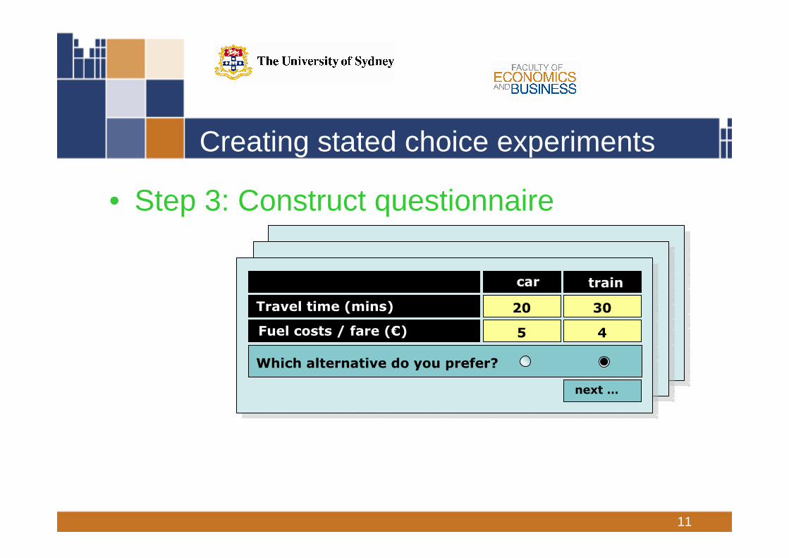
Creating stated choice experiments
• Step 3: Construct questionnaire
car train
20
5
30
4
Travel time (mins)
Fuel costs / fare (€)
Which alternative do you prefer?
next …

12
Experimental design
car train
Time Cost Time Cost
25 3 40 2
30 1 35 4
20 5 30 2
20 3 15 2
25 1 20 4
30 5 25 4
Given: number of alternatives, attributes, attribute levels/range
There are 3 x 3 x 6 x 2 = 108 possible different choice situations.
Full factorial designComplete set of all 108 choice situations.(typically too many for a single respondent)
Fractional factorial designSelect e.g. 6 choice situations from these possible 108 (gives 1,38·1012 potential designs)- orthogonal designs- efficient designs- other designs (constrained, pivot, …)

13
Full factorial designs
.
.
.
.
.
.
.
.
.
.
.
.
.
.
.
.
.
.
.
.
.
.
.
.
.
Advantages:- Includes all possible combinations of attribute levels- It can be used to estimate all main effects and interaction effects- Orthogonal (no correlations between attribute levels)
Disadvantages:- Too many questions for a single respondent- May contain “useless” choice situations
1 20 1 15 22 20 1 15 43 20 1 20 24 20 1 20 45 20 1 25 26 20 1 25 47 20 1 30 28 20 1 30 49 20 1 35 2
10 20 1 35 411 20 1 40 212 20 1 40 413 20 3 15 214 20 3 15 415 20 3 20 216 20 3 20 417 20 3 25 218 20 3 25 4
100 30 5 20 4101 30 5 25 2102 30 5 25 4103 30 5 30 2104 30 5 30 4105 30 5 35 2106 30 5 35 4107 30 5 40 2108 30 5 40 4

14
Orthogonal designs (traditional)
Advantages:- Orthogonal (no correlations between attribute levels)- Fractional factorial, so only a subset of choice situations
Disadvantages:- There may still be too many questions for a single respondent(the number of choice situations cannot be freely chosen)This problem may be solved by blocking.- It may not be possible to find an orthogonal design- May contain “useless” choice situations
1 20 3 35 22 25 5 15 23 30 1 25 24 25 3 25 45 30 5 35 46 20 1 15 47 20 1 30 28 25 3 40 29 30 5 20 2
10 30 1 20 411 20 3 30 412 25 5 40 413 25 1 15 214 30 3 25 215 20 5 35 216 30 5 40 417 20 1 20 418 25 3 30 419 25 5 30 420 30 1 40 421 20 3 20 422 30 3 35 423 20 5 15 424 25 1 25 425 25 5 20 226 30 1 30 227 20 3 40 228 20 1 40 229 25 3 20 230 30 5 30 231 30 3 15 432 20 5 25 433 25 1 35 434 20 5 25 235 25 1 35 236 30 3 15 2

15
Orthogonal designs (traditional)
Orthogonality may not be that important!
• orthogonality is usually lost in the data anyway, due to- missing blocks of observations- covariates (socio-economics, such as income or gender)
• orthogonality may not be important in estimating logit models,as it is the differences between the attribute levels that count
• non-orthogonal designs can yield more reliable parameter estimates

16
Optimal Orthogonal Choice Designs
• Optimal Orthogonal Designs (OOC) has been pioneered by Street (UTS)
• The aim of OOC designs is to:
• Maintain orthogonality in the design
• Within alternatives, not between alternatives
• Maximise the differences in the attribute levels across alternatives
• Force trade-offs between all attributes in every choice situation of the design

17
Optimal Orthogonal Choice Designs
• Optimal Orthogonal Designs (OOC) has been pioneered by Street (UTS)
• The aim of OOC designs is to:
• Maintain orthogonality in the design
• Within alternatives, not between alternatives
• Maximise the differences in the attribute levels across alternatives
• Force trade-offs between all attributes in every choice situation of the design

18
Optimal Orthogonal Choice Designs
http://survey.itls.usyd.edu.au/dating/SurveyController.php

19
Efficient designsAdvantages:- Fractional factorial, so only a subset of choice situations- More or less free choice in the number of choice situations(possibility to create smaller designs)- Aim to avoid “useless” choice situations- Improve the reliability of the parameter estimates
Disadvantages:- In general not orthogonal (not that important)- Prior parameter estimates (or prior distributions) are needed- Needs more computation power
1 20 5 35 22 25 5 25 23 30 3 20 24 25 1 40 45 30 3 30 46 20 1 15 4
1 30 3 15 42 30 1 35 43 30 1 20 44 20 1 25 45 25 5 30 26 20 3 35 27 20 1 20 48 25 3 40 29 25 5 25 2
10 20 5 15 211 30 5 30 212 25 3 40 4
20
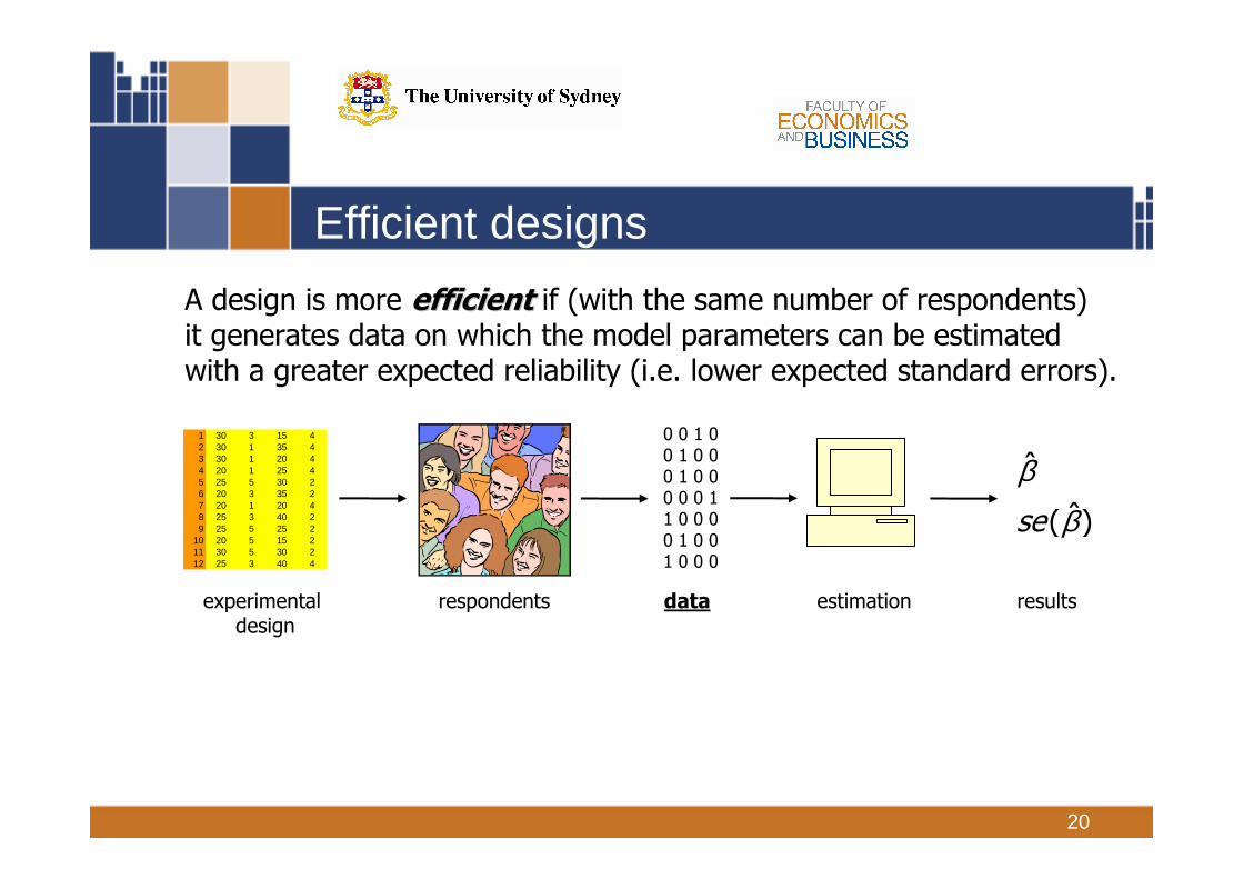
Efficient designs
A design is more efficientefficient if (with the same number of respondents)it generates data on which the model parameters can be estimatedwith a greater expected reliability (i.e. lower expected standard errors).
1 30 3 15 42 30 1 35 43 30 1 20 44 20 1 25 45 25 5 30 26 20 3 35 27 20 1 20 48 25 3 40 29 25 5 25 2
10 20 5 15 211 30 5 30 212 25 3 40 4
experimental design
respondents
0 0 1 00 1 0 00 1 0 00 0 0 11 0 0 00 1 0 01 0 0 0
data estimation
ββ
ˆ
ˆ( )se
results
21
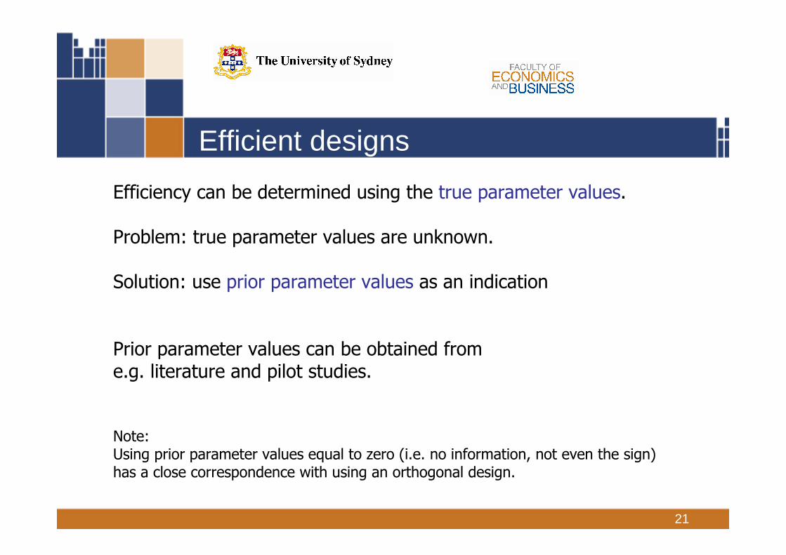
Efficient designs
Efficiency can be determined using the true parameter values.
Problem: true parameter values are unknown.
Solution: use prior parameter values as an indication
Prior parameter values can be obtained from e.g. literature and pilot studies.
Note: Using prior parameter values equal to zero (i.e. no information, not even the sign)has a close correspondence with using an orthogonal design.

22
Efficient designs
20 30
5 4
25 25
6 5
25 30
5 3
car train
20
3
30
6
Travel time (mins)
Fuel costs / fare ($)
car train
25
5
20
3
Travel time (mins)
Fuel costs / fare ($)
car train
30
3
25
4
Travel time (mins)
Fuel costs / fare ($)
= − ⋅ − ⋅= − ⋅ − ⋅0.2 0.05 0.1
0.04 0.1
car car car
train train train
U Time Cost
U Time Cost
= −= −0.9 (77%)
2.1 (23%)
car
train
U
U
= −= −1.3 (50%)
1.3 (50%)
car
train
U
U
= −= −1.2 (55%)
1.4 (45%)
car
train
U
U
Which choice situationwill provide the most information?
23
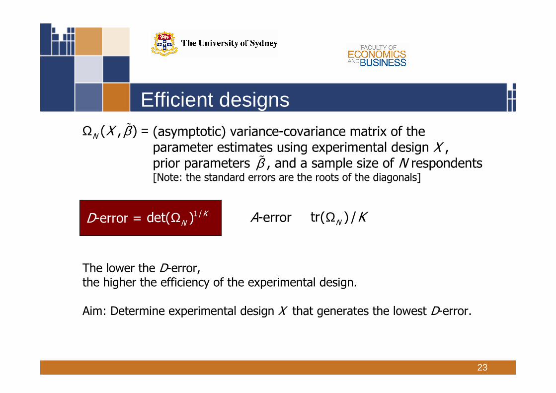
Efficient designs(asymptotic) variance-covariance matrix of the parameter estimates using experimental design X , prior parameters , and a sample size of N respondents[Note: the standard errors are the roots of the diagonals]
D-error = 1 /det( ) KNΩ
The lower the D-error, the higher the efficiency of the experimental design.
Aim: Determine experimental design X that generates the lowest D-error.
βΩ =( , )N X
β
Ωtr( ) /N KA-error =

24
Efficient designs
β β−
Ω = −
1
( , ) ( , )N NX I X
βββ β
∂=∂ ∂
2 ( , )( , )
'N
N
L XI X
β =( , )NL X Log-likelihood function
Determined (a) using Monte Carlo simulation, or(b) analytically

25
Efficient designs
β =∑∑∑( , ) logN isn isnn s i
L X y P
==1,
0,
isny if respondent n chooses alternative i in choice situation s
otherwise
=isnP probability that respondent n chooses alternative iin choice situation s

26
Efficient designs( )
( )β
β=∑exp ( , )
exp ( , )
i snisn
j snj
V XP
V X
( )
( )
( )( )
λ
λ
ββ
ββ
∈
∈∈
= ⋅
∑
∑∑ ∑
||
|
|
exp ( ,exp ( , )
exp ( , )exp ( , )
m
m
nk
m
k
jsn mj J isn m
isn
isn mj Jjsn k
k j J
V XV X
PV X
V X
( )( )β
ββ θ β
β= ∫∫∫ ∑
exp ( , )( | )
exp ( , )
i snisn
j snj
V XP g d
V X
MNL
NL
ML

27
Efficient designs
ββ β
∂ = − − ∂ ∂ ∑∑∑ ∑1 2 2
1 2
2* * *
* *
( , )ik sn isn ik sn jk sn jsn
n s i jk k
L Xx P x x P
ββ β
∂ = − − ∂ ∂ ∑∑ ∑1 1 1 1 2 2
1 1 2
2* *
*
( , )i k sn i sn i k sn jk sn jsn
n s ji k k
L Xx P x x P
( )β
β β
≠∂ = ∂ ∂ − − =
∑∑
∑∑
1 1 2 2 1 2
1 1 2 2 1 1 2 2 1 2
1 22
1 2
if ( , )
1 if
i k sn i k sn i sn i snn s
i k i k i k sn i k sn i sn i snn s
x x P P i iL X
x x P P i i
McFadden (1974)
Bliemer and Rose (2005)
MNL
Note: y drops out

28
Efficient designs
NL
β λ λβ β
λ λ λ
= = ∈ ∈ ∈
∈ = ∈
∂ = − − ∂ ∂
− − +
∑∑ ∑ ∑ ∑ ∑
∑ ∑ ∑
1 2 1 2
1 2 1 2 1 2
2 2 1
2 2
| | |1 1
| | |1
( ,( , ))( 1)
mk k mk mk
mk nk
S M
ms m mik s is m mik s mik s is m js m mjk sn s m i J i J j Jk k
M
m ms m is m mik s n ns is n nik s mik s is mi J n i J
L XP x P x x P P x
P P x P P x x P= ∈ ∈ ∈ ∈
− ∑ ∑ ∑ ∑ ∑1 2 1 2
1 1 2 1 2
| | |1 mk mk k mk mk
M
mik s is m mik s mik s is m js m mjk sm i J i J i J j J
x P x x P P x
β λ β λ λλ β = ∈ ∈ ∈ = ∈
∂ = − −
∂ ∂ ∑∑ ∑ ∑ ∑ ∑ ∑1 1 1 1 1 2 2
1 2 1 1 1 2 2
| |1 1
( ,( , ))log exp
m m i m k nk
S M
k m iks m s m is m m ik s n ns is n nik sn s i J k K i J n i Jm k
L Xx P P x P P x
( ) ββ λ
λ λβ β
= ∈ ∈
= ∈ ∈ ∈ ∈
− − =
∂ =∂ ∂
∑∑ ∑ ∑
∑ ∑ ∑ ∑
1 1 1
1 1
1 2
1 2 1 2
1 1 2 2
2
1 22 1
1
1 log exp , if ( ,( , ))
log exp log exp ,
m m i
m m i m m i
S
m s m s k m iksn s i J k K
m m S
m s m s k m iks k m ikss i J k K i J k K
P P x m mL X
P P x x
≠∑∑ 1 2if n
m m
Bliemer, Rose and Hensher (2006)
Note: y drops out

29
Efficient designsML Bliemer and Rose (2006)
Note: y drops out
( ) ( ) ( )( ) ( )
ϕ
ϕ ϕ
ϕ
µ σ ϕ ϕµ µ
ϕ ϕ ϕ ϕ
ϕ ϕ
∈ ∈ ∈ ∈
∈ ∈
∂ = − − − −∂ ∂
− ⋅ −−
∑∑ ∑ ∑ ∑ ∑∫
∑ ∑∫ ∫
∫
1 1 2 2 1 2 21 2 1 2
1 2
1 1 2 21 2
2 ( ,( , ))k k k k
k k
js jk s is ik s jk s is ik s js ik s is ik s hs hk si J i J i J h Js jk k
js jk s is ik s js jk s is ik si J i J
js
L XP x P x x P x P x P x P x d
P x P x d P x P x d
P d
( ) ( ) ( )( ) ( )
ϕ
ϕ ϕ
ϕ
µ σ ϕ ϕ ϕµ σ
ϕ ϕ ϕ ϕ ϕ
ϕ ϕ
∈ ∈ ∈ ∈
∈ ∈
∂ = − − − −∂ ∂
− ⋅ −−
∑∑ ∑ ∑ ∑ ∑∫
∑ ∑∫ ∫
∫
1 1 2 2 1 2 2 21 2 1 2
1 2
1 1 2 2 21 2
2 ( ,( , ))k k k k
k k
js jk s is ik s jk s is ik s js ik s is ik s hs hk s ki J i J i J h Js jk k
js jk s is ik s js jk s is ik s ki J i J
js
L XP x P x x P x P x P x P x d
P x P x d P x P x d
P d
( ) ( ) ( )( ) ( )
ϕ
ϕ ϕ
ϕ
µ σ ϕ ϕ ϕ ϕσ σ
ϕ ϕ ϕ ϕ ϕ
ϕ ϕ
∈ ∈ ∈ ∈
∈ ∈
∂ = − − − −∂ ∂
− ⋅ −−
∑∑ ∑ ∑ ∑ ∑∫
∑ ∑∫ ∫
∫
1 1 2 2 1 2 2 1 21 2 1 2
1 2
1 1 1 2 2 21 2
2 ( ,( , ))k k k k
k k
js jk s is ik s jk s is ik s js ik s is ik s hs hk s k ki J i J i J h Js jk k
js jk s is ik s k js jk s is ik s ki J i J
js
L XP x P x x P x P x P x P x d
P x P x d P x P x d
P d

30
Efficient designs
Interesting observation:
If all respondents face the same choice situations, then
1
1( , ) ( , )N X X
Nβ βΩ = Ω Hence, we can derive the asymptotic variance-covariance (AVC) matrix
with N respondents from the AVC matrix from a single respondent.
Furthermore:
β β= 1
1( , ) ( , )Nse X se X
N

31
Efficient designs
β( , )INse X
N
standard error
0 10 20 30 40 50
β1 ( , )Ise X
N
standard error
0 10 20 30 40 50
β( , )IINse X
β1 ( , )Ise X
β1 ( , )IIse X
Investing in more respondents Investing in better design
β( , )INse X

32
Efficient designs Bayesian efficient designs
Fixed values Probability distributions
What if the priors are unreliable?
traintraintrain
carcarcar
CostTimeU
CostTimeU
.~~
.~~~
23
210
βββββ
+=
++=
1.0~
2 −=β )0,5.0(~~
2 −Uβ
β2
Prob.
β2
Prob.
β2
Prob.
Instead of assumed fixed prior parameter values, we can assume prior parameter distributions.
or)05.0,1.0(~~
2 −Nβ

33
What if the priors are unreliable?Efficient designs:
Minimize D-error =
Bayesian efficient designs:
Minimize Expected D-error =
A Bayesian efficient design is a more “stable” design that willbe relatively efficient over a range of prior parameter values.
( )βΩ 1 /
det ( , )K
N X
( )β
β β ω βΩ∫∫∫
1 /
det ( , ) ( | )K
N X f d
This integral can be approximated by• pseudo-Monte Carlo simulation• Modified Latin Hybercube sampling• quasi-Monte Carlo simulation (e.g., Halton, Sobol draws)• Guassian quadrature

34
Other designs
Constrained designsSome attribute level combinations may not occur
Pivot designsAttribute levels pivoted from a knowledge base, so the design isoptimized for each individual or the whole population.
E.g. levels: [-50%, 0%, +50%]Respondent 1: travel time = 60 min. levels = 30, 60, 90Respondent 2: travel time = 10 min. levels = 5, 10, 15
Designs with covariatesAdding covariates (e.g. income, gender) to utility function changesthe efficiency of the design. One can create designs optimal foreach individual or the whole population.

35
How to generate designs?
Algorithms for finding efficient designs:
• Modified Federov algorithms• RSC (relabeling, swapping, cycling) algorithms•…

36
How to generate designs?
Step 1:Create canditure set
full / fractional factorial
Step 2:Create design by selecting choice situations from canditure set
design
Step 3:Compute efficiency error
D-error = ?
Step 4:Store design withlowest efficiencyerror next
iteration
Modified Federov Algorithm (Cook and Nachtsheim, 1980)

37
How to generate designs?
RSC Algorithm (Huber and Zwerina, 1996)
Step 1:Create columnsfor each attribute
Step 2:Create design by combiningthe columns for all attributes
Step 3:Compute efficiency error
D-error = ?
Step 4:Store design withlowest efficiencyerror next
iteration
design

38
Example
β β β ββ β β β β
= + + += + + + +
1 1 2 2 1 3 2 4
0 1 1 2 2 1 3 2 4
A A A A A A A
B B B B B B B B
V X X X X
V X X X X
β ββ ββ β β
= == == − = =
1 2
1 2
0 1 2
0.4 0.3
0.3 0.6
1.2 0.4 0.7A A
B B B
MNL model:
Priors:
Attribute levels:
= = = == = = =
1 11 2 3 42 2
1 11 2 3 42 2
2,4,6; 1,3,5; 2 ,3,3 ; 4,6,8;
2,4,6; 1,3,5; 2 ,4,5 ; 4,6,8.
A A A A
B B B B
X X X X
X X X X

39
Example
G1 G2 A1 A2 G1 G2 B0 B1 B21 4 3 2.5 4 6 3 1 4 82 2 3 3 6 4 1 1 5.5 63 2 5 3.5 4 6 5 1 2.5 84 4 1 2.5 8 2 3 1 4 45 6 1 2.5 8 2 3 1 5.5 66 6 5 3.5 6 6 5 1 2.5 47 2 5 2.5 4 4 5 1 5.5 88 4 1 3.5 4 6 1 1 2.5 69 2 3 3 6 2 1 1 5.5 8
10 6 1 3 8 2 1 1 4 411 4 5 3.5 6 4 5 1 2.5 412 6 3 3 8 4 3 1 4 6
correlation matrix:
G1 G2 A1 A2 G1 G2 B1 B2G1 1.00G2 -0.38 1.00A1 0.00 0.38 1.00A2 0.63 -0.50 -0.25 1.00G1 -0.13 0.50 0.50 -0.75 1.00G2 0.00 0.75 0.13 -0.25 0.38 1.00B1 -0.25 -0.25 -0.75 0.25 -0.63 -0.38 1.00B2 -0.63 0.25 -0.25 -0.63 0.25 0.00 0.38 1.00
D-error = 1.7470
“Random” design

40
Example
Orthogonal design
G1 G2 A1 A2 G1 G2 B0 B1 B21 4 1 3.5 6 2 3 1 4 42 2 1 3.5 8 6 5 1 4 83 2 3 3 4 6 1 1 5.5 44 2 3 3 6 2 3 1 2.5 45 4 3 3 6 2 3 1 5.5 86 6 1 2.5 4 4 5 1 5.5 67 6 5 3.5 8 4 1 1 5.5 68 6 1 2.5 8 4 1 1 2.5 69 4 5 2.5 8 6 5 1 4 4
10 6 5 3.5 4 4 5 1 2.5 611 4 3 3 4 6 1 1 2.5 812 2 5 2.5 6 2 3 1 4 8
correlation matrix:
G1 G2 A1 A2 G1 G2 B1 B2G1 1.00G2 0.00 1.00A1 0.00 0.00 1.00A2 0.00 0.00 0.00 1.00G1 0.00 0.00 0.00 0.00 1.00G2 0.00 0.00 0.00 0.00 0.00 1.00B1 0.00 0.00 0.00 0.00 0.00 0.00 1.00B2 0.00 0.00 0.00 0.00 0.00 0.00 0.00 1.00
D-error = 0.4251

41
ExampleEfficient design
G1 G2 A1 A2 G1 G2 B0 B1 B21 4 3 3 4 6 3 1 4 62 2 3 3 6 4 3 1 5.5 63 6 1 2.5 8 2 5 1 4 84 4 1 3.5 4 4 5 1 2.5 45 4 5 3.5 6 4 1 1 5.5 66 6 5 2.5 4 2 1 1 2.5 87 6 3 3 6 4 3 1 4 48 2 5 2.5 6 6 1 1 5.5 49 2 5 3.5 8 6 1 1 2.5 8
10 4 1 3.5 8 2 5 1 5.5 611 2 1 2.5 8 6 5 1 2.5 412 6 3 3 4 2 3 1 4 8
correlation matrix:
G1 G2 A1 A2 G1 G2 B1 B2G1 1.00G2 -0.13 1.00A1 -0.13 0.00 1.00A2 -0.38 -0.25 0.00 1.00G1 -0.75 0.25 0.00 0.13 1.00G2 0.13 -1.00 0.00 0.25 -0.25 1.00B1 -0.13 0.13 0.13 0.13 -0.13 -0.13 1.00B2 0.38 0.25 0.00 0.00 -0.50 -0.25 -0.13 1.00
D-error = 0.1949

42
Example
Orthogonal efficient design
correlation matrix:G1 G2 A1 A2 G1 G2 B0 B1 B2
1 4 5 3.5 8 6 1 1 4 82 4 3 3 4 6 5 1 2.5 43 2 5 3.5 6 2 3 1 4 44 6 1 3.5 8 4 5 1 2.5 65 4 1 2.5 6 2 3 1 4 86 6 5 2.5 4 4 1 1 2.5 67 6 1 3.5 4 4 1 1 5.5 68 6 5 2.5 8 4 5 1 5.5 69 2 3 3 4 6 5 1 5.5 8
10 2 3 3 6 2 3 1 2.5 811 4 3 3 6 2 3 1 5.5 412 2 1 2.5 8 6 1 1 4 4
G1 G2 A1 A2 G1 G2 B1 B2G1 1.00G2 0.00 1.00A1 0.00 0.00 1.00A2 0.00 0.00 0.00 1.00G1 0.00 0.00 0.00 0.00 1.00G2 0.00 0.00 0.00 0.00 0.00 1.00B1 0.00 0.00 0.00 0.00 0.00 0.00 1.00B2 0.00 0.00 0.00 0.00 0.00 0.00 0.00 1.00
D-error = 0.2918

43
Example
1.75
0.43
0.290.19
random orthogonal orth-efficient efficient
D-error
1.5 x
2.3 x
9.2 x

44
Example
1 1 3
2 3 2
4 4
, ,, ,,
A B B
A A B
A B
X X XX X XX X
3, 52, 45, 7
3, 4, 52, 3, 45, 6, 7
3, 3⅔, 4⅓, 52, 2⅔, 3⅓, 45, 5⅔, 6⅓, 7
2, 61, 54, 8
2, 4, 61, 3, 54, 6, 8
2, 3⅓, 4⅔, 61, 2⅓, 3⅔, 54, 5⅓, 6⅔, 8
1, 70, 63, 9
1, 4, 70, 3, 63, 6, 9
1, 3, 5, 70, 2, 4, 63, 5, 7, 9
attribute levels
1 1 3
2 3 2
4 4
, ,, ,,
A B B
A A B
A B
X X XX X XX X
1 1 3
2 3 2
4 4
, ,, ,,
A B B
A A B
A B
X X XX X XX X
narrow attribute level range wide
number of levels
β β β ββ β β β β
= + + += + + + +
1 1 2 2 1 3 2 4
0 1 1 2 2 1 3 2 4
A A A A A A A
B B B B B B B B
V X X X X
V X X X X
0.28 0.09 0.04
0.38 0.11 0.06
0.43 0.13 0.07
D-errors:

45
Optimal Choice Probability Designs
• Optimal choice percentage designs are basically D-efficient designs that are made more efficient by assuming that one attribute has continuous attribute levels (e.g., price)
• Pre-determined attribute levels (e.g., 1,3,5) put a constraint on the efficiency of a design; the efficiency could be improved if the attribute level is assumed continuous on a range (e.g., [1,5])

46
• Which choice situation yields the lowest D-error?
Optimal Choice Probability Designs (cont’d)
1 1 2 2
1 1 2 2
A
B
U A A
U B B
β ββ β
= += +
1
2
0.1
0.2
ββ
==
Model: Priors:
0.50, 0.50A BP P= =
0.01, 0.99A BP P= =
0.18, 0.82A BP P= =
0.40, 0.60A BP P= =

47
• In case of a generic model with two alternatives, the following optimal choice probabilities hold:
• What are the optimal probabilities for 3 or more alternatives?• What if the model is not generic?
Optimal Choice Probability Designs (cont’d)
Source: Johnson et al. (2006)
These probabilitiesare sometimes calledMagic P values

48
Generating Optimal Choice Prob. Designs
• Step 1: Generate orthogonal design for first alternative
• Step 2: Generate orthogonal designs for second alternative using a fold-over (reversing attribute levels)
• Step 3: Select attribute with continuous levels
• Step 4: Look up optimal choice probabilities from table
• Step 5: Change attribute levels of the continuous attribute such that in each choice situation these optimal choice probabilities are matched

49
Generating Optimal Choice Prob. Designs
• Consider generic model with 2 alternatives and 5 attributes (assume first attribute has continuous levels)
D-error = 3.5846
D-error = 0.2969
lowest D-error with fixed levels: 0.3750

50
Questions?
??
?
?
??
?
?
?? ?
?
??
?
?
??
?
?
??
?
?
??
??
?
?
?? ?
??
?

51
Thank you!


![[31] Designing Experiments Using Spotted Microarrays to](https://img.pdfslide.us/doc/110x75/61cedc675654e4620c490735/31-designing-experiments-using-spotted-microarrays-to-.jpg)