Graduate Theses and Dissertations Iowa State University Capstones, Theses andDissertations

2010

Designing effective and efficient incentive policiesfor renewable in generation expansion planningYing ZhouIowa State University

Follow this and additional works at: https://lib.dr.iastate.edu/etd

Part of the Industrial Engineering Commons

This Thesis is brought to you for free and open access by the Iowa State University Capstones, Theses and Dissertations at Iowa State University DigitalRepository. It has been accepted for inclusion in Graduate Theses and Dissertations by an authorized administrator of Iowa State University DigitalRepository. For more information, please contact digirep@iastate.edu.

Recommended CitationZhou, Ying, "Designing effective and efficient incentive policies for renewable in generation expansion planning" (2010). GraduateTheses and Dissertations. 11653.https://lib.dr.iastate.edu/etd/11653

Designing effective and efficient incentive policies for renewable energy in

generation expansion planning

by

Ying Zhou

A thesis submitted to the graduate faculty

in partial fulfillment of the requirements for the degree of

MASTER OF SCIENCE

Major: Industrial Engineering

Program of Study Committee:Lizhi Wang, Major Professor

Sarah M. RyanJames D. McCalley

Iowa State University

Ames, Iowa

2010

Copyright c© Ying Zhou , 2010. All rights reserved.

ii

DEDICATION

I would like to dedicate this thesis to my parents Fumin Zhou and Fengzhen Shao without

whose support I would not have been able to complete this work. I would also like to thank

my brother Qiang Zhou and friends for their loving guidance during the writing of this work.

iii

TABLE OF CONTENTS

LIST OF TABLES . . . . . . . . . . . . . . . . . . . . . . . . . . . . . . . . . . . v

LIST OF FIGURES . . . . . . . . . . . . . . . . . . . . . . . . . . . . . . . . . . vi

ACKNOWLEDGEMENTS . . . . . . . . . . . . . . . . . . . . . . . . . . . . . . vii

ABSTRACT . . . . . . . . . . . . . . . . . . . . . . . . . . . . . . . . . . . . . . . viii

CHAPTER 1. OVERVIEW . . . . . . . . . . . . . . . . . . . . . . . . . . . . . 1

1.1 Introduction to Policies for Renewable Energy . . . . . . . . . . . . . . . . . . . 1

1.1.1 Policies for renewable energy . . . . . . . . . . . . . . . . . . . . . . . . 1

1.1.2 Evaluation of an incentive policy . . . . . . . . . . . . . . . . . . . . . . 3

1.2 Bilevel Optimization for Incentive Policy Design . . . . . . . . . . . . . . . . . 3

1.3 Research Objective . . . . . . . . . . . . . . . . . . . . . . . . . . . . . . . . . . 5

1.4 Thesis Organization . . . . . . . . . . . . . . . . . . . . . . . . . . . . . . . . . 7

CHAPTER 2. REVIEW OF LITERATURE . . . . . . . . . . . . . . . . . . . 8

2.1 Generation Expansion Planning . . . . . . . . . . . . . . . . . . . . . . . . . . . 8

2.2 Policies for Renewable Energy . . . . . . . . . . . . . . . . . . . . . . . . . . . . 9

2.3 Inverse Optimization . . . . . . . . . . . . . . . . . . . . . . . . . . . . . . . . . 10

CHAPTER 3. MODELING AND ALGORITHM . . . . . . . . . . . . . . . . 11

3.1 GEP and Policy Design Modeling . . . . . . . . . . . . . . . . . . . . . . . . . . 11

3.1.1 Notations . . . . . . . . . . . . . . . . . . . . . . . . . . . . . . . . . . . 11

3.1.2 The generation expansion planning model . . . . . . . . . . . . . . . . . 14

3.1.3 The incentive policy design model . . . . . . . . . . . . . . . . . . . . . 17

3.1.4 The mandatory policy model . . . . . . . . . . . . . . . . . . . . . . . . 18

iv

3.2 Algorithm for Incentive Policy Design Model . . . . . . . . . . . . . . . . . . . 18

3.2.1 Definition of inverse mixed integer linear program . . . . . . . . . . . . 18

3.2.2 Cutting plane algorithm for inverse optimization . . . . . . . . . . . . . 19

3.2.3 Heuristic algorithm for incentive policy design model . . . . . . . . . . . 21

CHAPTER 4. CASE STUDY . . . . . . . . . . . . . . . . . . . . . . . . . . . . 24

4.1 Data Source . . . . . . . . . . . . . . . . . . . . . . . . . . . . . . . . . . . . . . 24

4.2 Implementation . . . . . . . . . . . . . . . . . . . . . . . . . . . . . . . . . . . . 28

4.3 Results . . . . . . . . . . . . . . . . . . . . . . . . . . . . . . . . . . . . . . . . . 28

4.3.1 Different cases of policies . . . . . . . . . . . . . . . . . . . . . . . . . . 28

4.3.2 Sensitivity analysis of the policies . . . . . . . . . . . . . . . . . . . . . . 33

CHAPTER 5. CONCLUSION AND FUTURE WORK . . . . . . . . . . . . 40

5.1 Conclusion . . . . . . . . . . . . . . . . . . . . . . . . . . . . . . . . . . . . . . 40

5.2 Future Work . . . . . . . . . . . . . . . . . . . . . . . . . . . . . . . . . . . . . 41

5.2.1 Future research on modeling . . . . . . . . . . . . . . . . . . . . . . . . 41

5.2.2 Further improvement of algorithm and data . . . . . . . . . . . . . . . . 41

5.2.3 Writing an open source software . . . . . . . . . . . . . . . . . . . . . . 41

BIBLIOGRAPHY . . . . . . . . . . . . . . . . . . . . . . . . . . . . . . . . . . . 42

v

LIST OF TABLES

Table 4.1 Coal supply network . . . . . . . . . . . . . . . . . . . . . . . . . . . . 25

Table 4.2 Existing electricity generation capacity . . . . . . . . . . . . . . . . . . 27

Table 4.3 Transmission data . . . . . . . . . . . . . . . . . . . . . . . . . . . . . . 27

Table 4.4 Cost of new coal and wind generation units . . . . . . . . . . . . . . . 27

vi

LIST OF FIGURES

Figure 1.1 Research objectives . . . . . . . . . . . . . . . . . . . . . . . . . . . . . 6

Figure 3.1 Illustration of AlgInvMILP . . . . . . . . . . . . . . . . . . . . . . . . . . 21

Figure 3.2 Heuristic algorithm for incentive policy design . . . . . . . . . . . . . . 22

Figure 4.1 Coal supply network . . . . . . . . . . . . . . . . . . . . . . . . . . . . 25

Figure 4.2 Electric power transmission model . . . . . . . . . . . . . . . . . . . . . 26

Figure 4.3 GEP costs under mandatory policy . . . . . . . . . . . . . . . . . . . . 30

Figure 4.4 GEP costs and taxes under tax policy . . . . . . . . . . . . . . . . . . 31

Figure 4.5 GEP costs and subsidies under subsidy policy . . . . . . . . . . . . . . 32

Figure 4.6 GEP costs and incentives under tax-subsidy policy . . . . . . . . . . . 34

Figure 4.7 GEP costs before and after coal production costs increase . . . . . . . 35

Figure 4.8 GEP costs before and after wind investment costs decrease . . . . . . 36

Figure 4.9 Incentives costs before and after wind investment costs decrease . . . 37

Figure 4.10 The total GEP costs in two situations . . . . . . . . . . . . . . . . . . 38

Figure 4.11 The total incentive costs in two situations . . . . . . . . . . . . . . . . 39

vii

ACKNOWLEDGEMENTS

I would like to take this opportunity to express my thanks to those who helped me with

various aspects of conducting research and the writing of this thesis. First and foremost, Dr.

Lizhi Wang for his guidance, patience and support throughout this research and the writing

of this thesis. His insights and words of encouragement have often inspired me and renewed

my hopes for completing my graduate education. I would also like to thank my committee

members for their efforts and contributions to this work: Dr. Sarah Ryan and Dr. James

McCalley. I would additionally like to thank my friends for their help during the writing of

this work.

viii

ABSTRACT

We present a bilevel optimization approach to designing effective and efficient incentive

policies for promoting renewable energy. The effectiveness of an incentive policy is its capability

to achieve a goal that would not be achievable without it. Renewable portfolio standard is

used in this thesis as the policy goal. The efficiency of an incentive policy is measured by

the amount of intervention, such as taxes collected and subsidies paid, to achieve the policy

goal. We obtain the most effective and efficient incentive policies in the context of generation

expansion planning, in which a planner makes investment decisions to serve project demand of

electricity. A case study is conducted on an integrated coal and electricity network representing

the contiguous United States. Numerical analysis from the case study provides insights on the

comparison of various incentive policies. The sensitivity of the incentive policies with respect

to coal production, energy investment costs, and transmission capacity is also studied.

1

CHAPTER 1. OVERVIEW

1.1 Introduction to Policies for Renewable Energy

Renewable energy is energy which comes from natural resources such as sunlight, wind,

rain, tides, and geothermal heat, which are renewable. Despite significant environmental and

social benefits, renewable energy is economically and technically disadvantaged [1]. In 2009,

President Barack Obama in the inaugural addresses called for the expanded use of renewable

energy to meet the twin challenges of energy security and climate change. The president’s plan

calls for renewable energy to supply 10% of the nation’s electricity by 2012, rising to 25% by

2025. In 2008, only 7% of the U.S. energy consumption came from renewable sources, with

84% from fossil fuels and 9% from nuclear [2].

Key barriers holding back the acceptance of renewable energy technologies, identified by

the Office of Energy Efficiency and Renewable Energy at DOE [3], include lack of government

policy support, high capital cost, and poor perception by public of renewable energy aesthetics.

Often the results of barriers is to put renewable energy at economic, regulatory, or institutional

disadvantage relative to other forms of energy supply.

1.1.1 Policies for renewable energy

In an effort to overcome these barriers, many countries around the world have implemented

various environmental policies [4, 5, 6, 7, 8], most of which belong to one of the three major

types:

• Mandates such as renewable portfolio standard (RPS), which is a regulation that requires

2

the increased production of energy from renewable energy sources, such as wind, solar,

biomass, and geothemal. As of June 2010, mandatory RPS policies have been passed

in 31 U.S. states and the the District of Columbia, with six additional states approv-

ing conditional or non-mandatory renewable goals. According to a new market study,

state renewable portfolio standards will be the most critical driver determining the pace

of U.S. renewable growth going forward. Meanwhile, state RPSs would be significantly

strengthened if complemented by a federal RPS or energy policy that addresses transmis-

sion bottlenecks which will be critical to sustaining renewable growth toward the middle

of the next decade.

• Incentives such as carbon tax, which is an environmental tax that is levied on the carbon

content of fuels. A carbon tax is a price instrument because it sets a price for carbon

dioxide emissions from burning of fossil fuels, such as coal, petroleum products such as

gasoline and natural gas. Accordingly, a carbon tax increases the competitiveness of non-

carbon technologies compared to the traditional burning of fossil fuels, to help protect

the environment.

• Markets such as cap-and-trade, which is a market-based approach used to control pollu-

tion by providing economic incentives for achieving reductions in the emission of pollu-

tants. Cap and trade is an environmental policy tool that delivers results with a manda-

tory cap on emission while providing sources flexibility in how they comply. Successful

cap and trade programs reward innovation, efficiency, and early action and provide strict

environmental accountability without inhibiting economic growth. Example of success-

ful cap and trade programs include the nationwide Acid Rain Program and the regional

NOx Budget Trading Program in the Northeast. Additionally, EPA issued the Clear Air

Interstate Rule (CAIR) on March 10, 2005, to build on the success of these programs

and achieve significant additional emission reductions.

3

1.1.2 Evaluation of an incentive policy

We evaluate the effectiveness of an incentive policy by its capability to achieve a renewable

portfolio standard, which requires a minimal percentage of electricity generation come from

renewable energy sources. This evaluation is conducted in the context of generation expansion

planning (GEP) [9, 10, 11, 12, 13, 14, 15], because the current installed renewable generation

capacity is far less than sufficient to meet the renewable portfolio standards set by many states

in America [16]. Without policy intervention, generation expansion planning in restructured

electricity markets is mainly profit-maximization and cost-minimization oriented [10], which

would lead to the least expensive – and most likely the least renewable – energy portfolio. An

effective policy would be able to improve the cost competitiveness of renewable energy in the

short term and accelerate technology development in the long term.

Besides effectiveness, cost efficiency is another important measure of an incentive policy,

which is based on how much intervention it takes to achieve a policy goal. The intervention

includes taxes collected, subsidies paid, or GEP cost increase as a result of the policies. The

less intervention it takes to achieve a goal, the more efficient a policy is, since taxes and GEP

cost increases need to be borne by the energy system and subsidies require expenditure of tax

payers’ money. Cost efficiency of renewable energy policies is a worldwide grand challenge

[17, 18, 19, 20, 21], especially under the current economy.

1.2 Bilevel Optimization for Incentive Policy Design

We presents a novel bilevel optimization approach to designing effective and efficient in-

centive policies.

A typical optimization problem is a forward problem since it needs to find an optimal given

the values of parameters, which include cost coefficients and constraints. Inverse optimization

[27, 28, 30, 35, 37] is a branch of bilevel optimization that deals with finding a minimal pertur-

bation of the objective function of an optimization problem in order to make a target solution

4

optimal.

In the GEP context, the target solution is an expansion strategy that represents a health-

ier tradeoff between economic benefit and environmental impact but would not be optimal

under a cost-minimization framework, and the minimal perturbation is the most efficient in-

centive policy that could make the target expansion strategy become optimal under the policy

intervention. Let the GEP problem be represented with the following mixed integer linear

program

min c>x (1.1)

s. t. Ax ≥ b (1.2)

x ≥ 0, xI ∈ Z|I|, (1.3)

where A ∈ Rm×n, b ∈ Rm, c ∈ Rn, and I ⊆ {1, ..., n}. Without any policy intervention,

suppose x∗ is the optimal solution to the GEP (1.1)-(1.3), which can be expected to include

little or no investment in renewable energy.

Suppose our target investment strategy is required to satisfy an additional constraint

Hx ≤ h, which is represents the policy effectiveness requirement, such as including a healthier

portfolio of investment in renewable and non-renewable energy. The incentive policy design

problem can be mathematically posed as to find a minimal incentive perturbation ∆c, measured

by some norm f(∆c, x), such that the target solution x becomes optimal to the incentivized

GEP:

minx,∆c

f(∆c, x) (1.4)

s. t. Hx ≤ h (1.5)

x ∈ argminx{(c+ ∆c)>x : Ax ≥ b, x ≥ 0, xI ∈ Z|I|}. (1.6)

5

1.3 Research Objective

Many [22, 23, 25, 26] studies have analyzed the environmental policies adopted at the fed-

eral and/or state level for promoting renewable energy. Most of these studies focus on the

consequences and implications of the policies. The main objective of our research is to address

a perhaps more fundamental issue: how the policies should be designed in the first place to be

most effective and efficient?

The first objective is to present efficient and efficiency incentive policies design models.

For such purpose, recent advances [27, 28] in inverse optimization have provided suitable mod-

eling tools. In [29], we introduced an earlier and over simplified inverse optimization model

for incentive policy design, in which the target investment strategy is supposed to be exoge-

nously determined rather than endogenously obtained by the model. The models presented

here extend such unrealistic limitation and provide a more powerful decision tool to not only

design incentive policies but also obtain the optimal investment tradeoff. Here constraint (??)

enforces the effectiveness of the policy, constraint (1.6) anticipates the consequences of the pol-

icy, and objective (1.4) minimizes the policy intervention (thus maximize the policy efficiency).

The second objective is to present new algorithm for the incentive policy design models.

The incentive policy design model is a complex bilevel problem, in which the the upper level

has a nonlinear nonconvex objective function and the lower level involves both continuous and

discrete decision variables. As far as we are aware of, there are no existing algorithms for

solving bilevel problems of such complexity. We try to propose a heuristic algorithm for this

problem.

The third objective is to demonstrate our models and solution techniques through a case

study, which is an integrated coal and electricity network of the U.S. continent with real his-

torical data. We compare the effectiveness and efficiency of the mandatory renewable portfolio

standard and several incentive policies, representing the production tax credit, investment tax

6

Figure 1.1 Research objectives

credit, carbon taxes, etc.

In summary, the objectives are to:

• Design incentive policies to stimulate the renewable energy’s development to overcome

the limitations of existing policies.

• Present efficient algorithm to solve the incentive policy design models based on the ex-

isting algorithm for the inverse optimization.

• Demonstrate our models and solution techniques through a case study and analyze the

sensitivity of our models.

7

1.4 Thesis Organization

Chapter 2 reviews the relevant literatures about the generation expansion planning, policies

for renewable energy and inverse algorithm. Chapter 3 introduces the incentive policy design

and mandatory policy models and proposes a heuristic algorithm for the incentive policy de-

sign model. Chapter 4 presents a case study on an integrated coal and electricity networks.

Algorithm implementation, computational experiment results are reported. Conclusion and

future research follow in Chapter 5.

8

CHAPTER 2. REVIEW OF LITERATURE

In this chapter, we review some literatures on models for GEP, government incentive poli-

cies and inverse optimization.

2.1 Generation Expansion Planning

The optimization models for GEP include: game-theoretic models, stochastic programming

models and multiobjective models etc. Chuang et al. [11] and Murphy et al. [15] apply the

Cournot model of oligopoly to model GEP. The model of Chuang et al. incorporate plant

capacity limitations and energy balance constraint in competitive environments dominated by

auction markets. They present an analytical formulation of the generation planning process

involving decisions on new plant construction at a single point in time with multiple technol-

ogy options available. Murphy et al. analyze three capacity expansion models in the context

of a restructured electricity industry. The first model assumes a perfect, competitive equilib-

rium. The second model (open-loop Cournot game) extends the Cournot model to include

investments in new generation capacities. The third model (closed-loop Cournot game) sep-

arates the investment and sales decision with investment in the first stage and sale in the

second stage. Mo et al. [14] and Lopez et al. [12] model the GEP using stochastic program-

ming. Mo et al. provide a method using Markov Chains to handle some uncertainties such

as energy demand and prices of energy carriers. The new model can construct a connection

between investment decision, time, construction periods, and uncertainty. Lopez et al. present

a stochastic programming with probabilistic constraints to consider random events in genera-

tion and transmission expansion. Meza et al. [13], Antunes et al. [10] and Ahmed et al. [9]

9

propose a multiobjective model for generation expansion planning (MGEP). The objectives

of the model in [13] are the minimization of investment, operation and transmission costs,

environment impact, imports of fuel and fuel prices risks of the whole system. Multiobjective

linear programming and analytical hierarchy process are made use of to solve this problem.

The model of Antunes et al. is presented to provide decision support in the evaluation of power

generation capacity expansion policies. The objective functions are the total expansion cost,

the environmental impact associated with the installed power capacity and the environmental

impact associated with the energy output. Ahmed et al. use a scenario tree approach to

model the evolution of uncertain demand and cost parameters, and fixed-charge cost function

to model the economies of scale in expansion costs.

2.2 Policies for Renewable Energy

There exists a vast literature on policies to support renewable energy and reduce gas emis-

sion. We list five policies: generation subsidy for renewable energy [5, 23], tax on fossil fuel

energy [24], portfolio standards [7], subsidies for R&D [8, 26] and price on carbon [6]. Loiter

and Norberg-Bohm [23] present a study of technological and policy history of the develop-

ment of wind power in the United States. Greenberg and Murphy [5] provide a framework

for representing selected price-oriented government regulations in mathematical programming

model of a market. Roy et al. [24] evaluate the cost and benefits of energy taxation as a

policy instrument to conserve energy and reduce CO2 emissions. Rader and Norgaard [7] pro-

vide the correct use of economics can fashion policies to structure the market so that social

goal of reliability, environmental quality and equity are attained most efficiently. Nemet and

Baker [26] compare effects of R&D and demand subsidies on the future costs of purely organic

photovoltaics (PV) which is not currently commercially available. They combine an expert

elicitation and a manufacturing cost model to compare the outcomes of policy choices over

various scenarios. Solomon and Banerjee [8] survey the global status of hydrogen energy re-

search and devlopment (R&D) and public policy. Goulder [6] considers alternative tax designs

10

that different according to the tax treatment of internationally trades goods and the use of tax

revenues.

2.3 Inverse Optimization

Inverse problems originated from geophysical sciences [30], in which the values of model pa-

rameters must be inferred from values of given observable parameters. Since Burton and Toint

published their paper on an instance of the inverse shortest paths problem, inverse problems

have been studied extensively by researchers. There has been a number of papers concerning

inverse optimization problems, such as inverse linear programming [31], inverse maximum flow

and minimum cut [32], inverse minimum assignment [31], inverse minimum spanning tree [33],

inverse shortest arborescence [34], etc. The purpose of these inverse problems is to make mini-

mum change on the parameters in these problems so that a given feasible solution will become

the optimal one. Existing studies [35, 37] of inverse optimization have mainly focused on in-

verse linear programming problems, in which the lower level optimization is a linear program.

The inverse linear programming problem has first been investigated by [36]. They formulate

the inverse linear programming problem as a new linear program. Wang [28] extends this

model to inverse mixed integer linear programming problems, which allow the lower level to

contain integer variables as well as continuous ones. This is particularly important for GEP,

in which the discrete nature of some investment decisions must be taken into account.

11

CHAPTER 3. MODELING AND ALGORITHM

3.1 GEP and Policy Design Modeling

In this section, we present our incentive policy design model, which consists of two levels of

optimization. At the lower level, a central decision maker is supposed to expand the generation

capacity of an energy system to serve projected load with minimum total cost, including both

generation costs and investment costs. At the upper level, a policy maker aims to influence

the decision of the lower level planner by applying incentive policies. We also introduce a

mandatory policy model, in which the generation expansion planner is required to have a

certain percentage of power generation from renewable sources. The notations used in this

section are are summarized in Section 3.1.1. The optimization models of the GEP and incentive

policy design are presented in Sections 3.1.2 and 3.1.3, respectively.

3.1.1 Notations

Sets

• I: Set of coal production nodes.

• J : Set of electricity generation nodes.

• K: Set of transportation links that connect nodes in I and nodes in J .

• L: Set of transmission lines that connect nodes in J .

Parameters

• Gi: Coal production capacity (ton) at node i ∈ I.

12

• PCi : Coal production cost ($/ton) at node i ∈ I.

• Fk: Coal transportation capacity (ton) at link k ∈ K.

• P Tk : Coal transportation cost ($/ton) at link k ∈ K.

• AC , AE : Rows in the node-arc incidence matrix in the undirected network comprised of

{I ∪ J ,K} that correspond to nodes I and J , respectively.

• Dj : Average electricity demand (MW) at node j ∈ J .

• BCj : Overnight investment cost ($) of new coal generation units at node j ∈ J .

• BWj : Overnight investment cost ($) of new wind generation units at node j ∈ J .

• V Cj : Variable operating and maintenance (O&M) cost ($/MWh) for existing coal gener-

ation units at node j ∈ J .

• V Wj : Variable O&M cost ($/MWh) for existing wind generation units at node j ∈ J .

• V NCj : Variable O&M ($/MWh) cost of new coal generation units at node j ∈ J .

• V NWj : Variable O&M ($/MWh) cost of new wind generation units at node j ∈ J .

• FCj : Fixed variable O&M ($/MW) cost of new coal generation units at node j ∈ J .

• FWj : Fixed variable O&M ($/MW) cost of new wind generation units at node j ∈ J .

• QCj : Total capacity (MW) of the existing coal generation units at node j ∈ J .

• QWj : Total capacity (MW) of the existing wind generation units at node j ∈ J .

• ∆QCj : Total capacity (MW) of one new coal generation unit at node j ∈ J .

• ∆QWj : Total capacity (MW) of one new wind generation unit at node j ∈ J .

• Tl: Capacity of transmission line l ∈ L.

13

• H: Power transfer distribution factors (PTDF) matrix. PTDF matrix gives the linear

relation between net injection at each node and power flow through line. Net injection

is the total power flow going into a node less the total power flow going out of it.

• α: Tonnage of coal needed to generate one MWh of electricity (ton/MWh).

• RC : Discount factor of overnight investment cost for new coal generation units.

• RW : Discount factor of overnight investment cost for new wind generation units.

• r: Percentage requirement of a renewable portfolio standard.

Lower Level Decision Variables

• fk: Quantity (ton) of coal transported through link k ∈ K.

• gi: Quantity (ton) of coal production at node i ∈ I.

• xj : Quantity (MWh) of electricity generated by existing coal generation units at node

j ∈ J .

• yj : Quantity (MWh) of electricity generated by existing wind generation units at node

j ∈ J .

• ∆xj : Quantity (MWh) of electricity generated by new coal generation units at node

j ∈ J .

• ∆yj : Quantity (MWh) of electricity generated by new wind generation units at node

j ∈ J .

• NCj : Integer number of new coal generation units at node j ∈ J .

• NWj : Integer number of new wind generation units at node j ∈ J .

Upper Level Decision Variables

• sBW

j : Investment subsidy policy ($) for new wind generation units at node j ∈ J .

14

• sV W

j : Production subsidy policy ($) for existing wind generation units at node j ∈ J .

• sV NW

j : Production subsidy policy ($) for new wind generation units at node j ∈ J .

• tBC

j : Investment tax policy ($) for coal generation units at node j ∈ J .

• tV C

j : Production tax policy ($) for existing coal generation units at node j ∈ J .

• tV NC

j : Production tax policy ($) for new coal generation units at node j ∈ J .

3.1.2 The generation expansion planning model

In a GEP problem, a planner aims to expand the generation capacity of an energy system

to serve projected load with minimum cost. The energy system we consider consists of an

electricity generation/transmission network and a coal production/transportation network.

In the electricity network, we use J to denote the set of electricity generation nodes and

L the set of transmission lines that connect these nodes. In the coal network, I is the set of

coal production nodes and K is the set of transportation links that connect coal nodes I an

electricity nodes J .

At each coal production node i ∈ I, the coal production capacity is Gi (ton) and the cost

is PCi ($/ton). For each link k ∈ K, the transportation capacity is Fk (ton) and the trans-

portation cost is P Tk ($/ton).

At each electricity generation node j ∈ J , the overnight investment costs of new coal and

wind generation units are BCj ($) and BW

j ($), respectively. RCj and RW

j are the respective

discount factors that convert the lump sum costs to hourly costs. The variable O&M costs

of new coal and wind generation units are V NCj ($/MWh) and V NW

j ($/MWh), respectively.

The fixed variable O&M costs of new coal and wind generation units are FCj ($/MW) and FW

j

($/MW), respectively. The capacity of one additional coal or wind generation unit is ∆QCj

15

(MW) or ∆QWj (MW), respectively.

In the undirected network defined by N = {I ∪ J ,K}, we use AC and AE to denote the

rows in the node-arc incidence matrix that correspond to nodes I and J , respectively. At each

node j ∈ J , the average electricity demand is Dj (MWh); the total capacity of the existing coal

generation units is QCj (MW); the total capacity of the existing renewable generation units is

QWj (MW); variable operating and maintenance (O&M) cost for existing coal generation units

is V Cj ($/MWh); the variable O&M cost for existing renewable power generation units is V W

j

($/MWh). For each link l ∈ L, Tl (MW) is the capacity of transmission line l. We denote H

as the power transfer distribution factors (PTDF) matrix and α (ton/MWh) as the tonnage

of non-renewable needed to generate a MWh of electricity.

We introduce the decision variables in the GEP model as follows. At each coal production

node i ∈ I, gi (ton) is the quantity of coal production. For each link k ∈ K, fk (ton) is the

quantity of coal transported through link k ∈ K. At each electricity generation node j ∈ J ,

xj , yj , ∆xj , and ∆yj are MWh of electricity generation by existing coal, existing wind, new

coal, and new wind generation units, respectively. NC and NW are integer number of new

coal and wind generation units. The base case GEP model can be formulated as the following

mixed integer linear program.

16

min (PC)>g + (P T )>f + (V C)>x+ (V NC)>∆x+ (V W )>y + (V NW )>∆y

+(RCBC + FC)>∆QCNC + (RWBW + FW )>∆QWNW (3.1)

s. t. α(x+ ∆x) ≤ AEf (3.2)

g = ACf (3.3)

H(x+ ∆x+ y + ∆y −D) ≤ Tl (3.4)

1>(x+ ∆x+ y + ∆y −D) = 0 (3.5)

0 ≤ ∆x ≤ ∆QCNC (3.6)

0 ≤ ∆y ≤ ∆QWNW (3.7)

0 ≤ x ≤ QC (3.8)

0 ≤ y ≤ QW (3.9)

0 ≤ f ≤ F (3.10)

0 ≤ g ≤ G (3.11)

NC , NW integer. (3.12)

The objective function (3.1) is to minimize total GEP costs, including coal production

and transportation cost, fixed and variable O&M cost, and discounted overnight investment

cost. Constraint (3.2) is the coal supply capacity for electricity generation; (3.3) equates coal

production and the amount available for transportation; (3.4) is the electricity transmission

capacity limit; (3.5) is the network conservation constraint; (3.6) is the capacity of new coal

generation units; constraint (3.7) is the capacity of new wind generation units; constraint (3.8)

is the capacity of existing coal generation units; (3.9) is the capacity constraint of existing wind

generation units; (3.10) is the capacity constraint of existing coal transportation; (3.11) is the

capacity constraint of coal production; and (3.12) requires that the number of new generation

units be an integer.

17

3.1.3 The incentive policy design model

The incentive policy design model is a bilevel optimization problem. The lower level is a

GEP problem under tax and/or subsidy intervention:

min (PC)>g + (P T )>f + (V C + tVC

)>x+ (∆V C + tVNC

)>∆x

+(V W − sV W)>y + (V NW − sV NW

)>∆y

+(RCBC + FC + tBC

)>∆QCNC + (RWBW + FW − sBW)>∆QWNW (3.13)

s. t. Constraints (3.2)-(3.12). (3.14)

Here tVC, tV

NC, tB

Care the taxes on x,∆x,NC , and sV W

, sV NW, sBW

are the subsidies on

y,∆y,NW , respectively.

The upper level’s incentive policy design model is

min (tVC

)>x+ (tVNC

)>∆x+ (tBC

)>∆QCNC

+(sV W)>y + (sV NW

)>∆y + (sBW)>∆QWNW

+(PC)>g + (P T )>f + (V C)>x+ (V NC)>∆x+ (V W )>y + (V NW )>∆y

+(RCBC + FC)>∆QCNC + (RWBW + FW )>∆QWNW

−constant (3.15)

s. t. 1>(y + ∆y) ≥ r · 1>(x+ ∆x+ y + ∆y) (3.16)

{x,∆x, y,∆y,NW , NC} ∈ argmin{(3.13) : Constraints (3.2)-(3.12)}. (3.17)

The objective function (3.15) is to minimize the total cost of policy intervention, including

taxes collected (first line), subsidies paid (second line), and the GEP cost increase (third and

fourth lines). The constant term is the GEP cost without policy intervention calculated from

(3.1)-(3.12). Constraint (3.16) uses the renewable portfolio standard that require 100r% as the

implicit policy goal, and (3.17) is the anticipated response from the lower level.

18

3.1.4 The mandatory policy model

We also present the GEP under mandatory policy model to provide a benchmark com-

parison. In this model, no taxes or subsidies are imposed to the objective function, but the

renewable portfolio standard is explicitly enforced to the GEP problem as an additional con-

straint:

min Objective (3.1) (3.18)

s. t. 1>(y + ∆y) ≥ r · 1>(x+ ∆x+ y + ∆y) (3.19)

Constraints (3.2)-(3.12). (3.20)

3.2 Algorithm for Incentive Policy Design Model

The base case GEP model (3.1)-(3.12) and the GEP under mandatory policy model (3.18)-

(3.20) are mixed integer programs, for which there exist efficient solvers. However, the incentive

policy design model (3.15)-(3.17) is a complex bilevel problem, in which the upper level has

a nonlinear non-convex objective function and the lower level involves both continuous and

discrete decision variables. As far as we are aware of, there are no existing algorithms for

solving bilevel problems of such complexity. In this section, we propose a heuristic algorithm

for this problem.

We first introduce a revised version of the cutting plane algorithm from [28] for solving the

inverse mixed integer linear programming (InvMILP) problem, and then present the heuristic

algorithm that uses the InvMILP algorithm as a subroutine to solve the incentive policy design

problem (3.15)-(3.17).

3.2.1 Definition of inverse mixed integer linear program

Let IP(A, b, c, I) denote an instance of mixed integer linear program (MILP)

maxx{c>x : Ax ≤ b, x ≥ 0, xI ∈ Z}, (3.21)

19

where A ∈ Rm×n, b ∈ Rm, c ∈ Rn, and I ⊆ {1, ..., n}. An InvMILP is to minimally perturb c

in order to make the given feasible solution xd optimal. In other words, it’s to find a direction

d that satisfies two conditions. Firstly, the direction d makes given feasible solution xd optimal

to MILP ([28]); secondly, the difference between c and d, measured by ||c − d||, is minimal

among all the directions that can make xd optimal. In this thesis, we focus our discussion on

the weighted L1 norm, so ||c− d|| becomes w>|c− d|, where w ∈ Rn+ is a constant vector. The

straightforward formulation of the InvMILP under the weighted L1 norm is

mind{w>|c− d| : xd ∈ argmaxx{d>x : Ax ≤ b, x ≥ 0, xI ∈ Z}}. (3.22)

3.2.2 Cutting plane algorithm for inverse optimization

We first introduce a revised version of the cutting plane algorithm from ([28]) for solving

the InvMILP, which we refer to as AlgInvMILP. The AlgInvMILP algorithm solves InvMILP

problems defined as follows. For a given solution x ∈ Rn to the mixed integer linear program

(1.1)-(1.3), find a minimal intervention t, s ∈ Rn+, measured by x>(t+ s), such that x becomes

an optimal solution to min{(c+ t− s)>x : constraints (1.2)-(1.3)}:

min x>(t+ s) (3.23)

s.t. x ∈ argmin{(c+ t− s)>x : constraints (1.2)-(1.3)}. (3.24)

Here t and s represent tax and subsidy policies, respectively, and the objective function (3.23)

is to minimize the dollar amount of incentive policy intervention, either as subsidies paid to

wind generation or taxed collected from coal generation. The AlgInvMILP algorithm consists of

the following steps.

Step 0: Initialize S0 = ∅.

20

Step 1: Let (y∗, t∗, s∗) be an optimal solution to the following linear program:

miny,t,s

x>t+ x>s (3.25)

s. t. A>y ≤ c+ t− s (3.26)

(c+ t− s)>x ≤ (c+ t− s)>x0, ∀x0 ∈ S0 (3.27)

y, t, s ≥ 0. (3.28)

Step 2: Let x0 be an optimal solution to min{(c + t∗ − s∗)>x : Ax ≥ b, x ≥ 0, xI ∈ Z|I|}. If

(c+ t∗ − s∗)>x ≤ (c+ t∗ − s∗)>x0, then stop. Otherwise update S0 = S0 ∪ {x0} and go

back to Step 1.

Theorem 1. AlgInvMILP terminates finitely with an optimal solution to InvMILP (3.22) [28].

Remark 1. In Step 0, S0 is initialized, which denotes the set of known extreme points

of the convex hull of {Ax ≤ b, x ≥ 0, xI ∈ Z|I|}. The set S0 will be updated as new extreme

points are discovered. Step 1 generates a lower bound solution (c+t∗−s∗) that has the minimal

intervention but may or may not make x optimal. Therefore, Step 2 checks the optimality of

x with respect to min{(c + t∗ − s∗)>x : Ax ≥ b, x ≥ 0, xI ∈ Z|I|}. If the answer is positive,

then (t∗, s∗) is proved to be the optimal solution to (3.23)-(3.24); otherwise a new extreme

point x0 is generated and added to the set S0. The Step 1-Step 2 loop continues until the

optimality of x is confirmed in Step 2. A detailed proof of finite convergence of AlgInvMILP to

exact optimality can be found in [28].

Remark 2. Tax only or subsidy only policies can be modeled by adding additional con-

straints s = 0 or t = 0 to (3.25)-(3.28), respectively.

Remark 3. Although this algorithm is proved in [28] to finitely converge to the optimal

solution to (3.23)-(3.24), it is insufficient to solve the incentive policy design model (3.15)-

(3.17). This is because the algorithm only finds the optimal incentive policy for a prescribed

GEP solution x, but the incentive policy design model needs to find the optimal GEP solution

21

endogenously rather than take it as exogenously provided. As illustrated in Figure 3.1, the

GEP problem is inherently cost minimization oriented. Therefore, an incentive policy (t, s) is

indispensable to achieve any GEP solution x that compromises cost efficiency for more renew-

able energy. The incentive policy design model (3.15)-(3.17) requires both an optimal GEP

solution x and the most efficient policy (t, s) to achieve it.

cost6

renewable-

sxc

s xs s s s?

cJ

JJJ

c+ t− s

Figure 3.1 Illustration of AlgInvMILP

3.2.3 Heuristic algorithm for incentive policy design model

In the incentive policy design problem (3.15)-(3.17), the lower level’s decisions are not pre-

determined except that they should satisfy constraint (3.19), so the above algorithm does not

directly solve this problem. We propose the following heuristic algorithm for problem (3.15)-

(3.17):

Step A: Obtain 1001 GEP solutions. The first 1000 solutions are optimal solutions to

(3.13)-(3.14) with 1000 randomly generated incentive policies (sV W, sV NW

, sBW, tV

C, tV

NC, tB

C).

22

The 1001st solution is an optimal solution to the GEP under mandatory policy model (3.18)-

(3.20).

Step B: For each GEP solution, treat it as x and use the AlgInvMILP algorithm to obtain

the optimal incentive. Among the 1001 incentive policies, choose the optimal one with respect

to objective (3.15).

Figure 3.2 Heuristic algorithm for incentive policy design

Remark 4. The need for the above heuristic algorithm is justified by two major difficulties

of the model (3.15)-(3.17). First, the lower level contains both continuous and discrete decision

variables. In a GEP problem, many investment decisions are inherently discrete, e.g., the deci-

23

sion to invest in a new wind farm in a specific location will incur a significant amount of capital

cost that is independent of and non-proportional to the magnitude of generation capacity. This

difficulty can be mitigated to some extent by ignoring the integrality constraints, which will

reduced the constraint (3.17) to its complementary slackness conditions. The second difficulty

with model (3.15)-(3.17) is the non-convexity and nonlinearity of the objective function (3.15).

This is much more serious than the first one because there exists a finitely converging ex-

act algorithm for the model with a linear objective function, but even integrality constraints

are relaxed, the resulting model is still a nonlinear non-convex mathematical program with

complementary constraints, for which even a local optimal solution is in general extremely

hard to obtain. The heuristic algorithm we present tries to fish a good solution by randomly

generating a large number of GEP solutions and then comparing their corresponding optimal

incentive policies. A GEP solution will linearize the objective function (3.15) and make the

model finitely solvable to global optimality by AlgInvMILP.

24

CHAPTER 4. CASE STUDY

In this section, we conduct a case study on an integrated energy system that consists of elec-

tricity generation/transmission and coal production/transportation networks. The integrated

network represents the contiguous United States, which consists of 17 electricity generation

nodes, 11 coal production nodes, 29 electricity transmission lines, and 187 transportation links

connecting every coal production node with every electricity generation node.

4.1 Data Source

The coal network is illustrated in Figure 4.1 (data source: Energy Information Adminis-

tration [2]). Table 4.1 summarizes the supply regions that the coal supply nodes represent

as well as their production capacity and average minemouth price (data source: [38, 39, 40]).

The electricity generation network is illustrated in Figure 4.2 and the regions that the nodes

represent are summarized in Table 4.2 (data source: [41]). Table 4.2 also gives the supply and

demand of electricity. Electricity transmission capacity data are given in Table 4.3. Table 4.4

presents overnight investment, variable O&M, and fixed O&M costs, which are obtained from

[42]. We use α as 0.2.

25

Figure 4.1 Coal supply network

Table 4.1 Coal supply network

Supply node RegionProductive capacity Average minemouth

(103 tons) price (2002 $/ton)A Northwest 8,166 15.90B Powder River Basin 53,581 17.48C Rocky Mountains 70,508 22.61D Southwest 44,173 19.78E North Dakota Lignite 33,500 13.27F Other Western Interior 3,228 23.28G Gulf Coast Lignite 54,549 13.03H Illinois Basin 114,917 22.10I Northern Appalachia 167,772 24.01J Central Appalachia 317,957 25.21K Southern Appalachia 29,661 25.36

26

Figure 4.2 Electric power transmission model

27

Table 4.2 Existing electricity generation capacity

Node j Region QCj QW

j Dj

1 Northwest 1,241 2,765 13,6602 California 34 2,537 17,2343 Arizona-New Mexico-Southern Nevada 552 496 8,0574 Rocky Mountain 1,190 1,527 3,5555 Mid-Continent 6,672 478 9,9406 Southwest 8,420 1,199 13,5477 Texas 3,317 6,698 19,7728 Mid-America 15,134 3,256 18,9049 East Central 22,195 300 36,70410 Energy Electric System 3,981 1 9,29111 Tennessee Valley Authority 4,067 29 10,75612 Virginia-Caolinas 7,006 0 21,58613 Southern Company 9,587 0 15,79514 Florida Reliability Coordinating 1,785 0 14,81915 Mid-Atlantic Area Council 7,317 374 19,13616 New York ISO 1,326 6 11,02917 ISO New England 973 43 9,137

Table 4.3 Transmission data

Link l Tl Link l Tl Link l Tl Link l Tl

1-2 6,820 1-3 1,140 1-4 3,050 1-5 1504-5 310 3-4 650 2-3 9,965 3-6 4205-6 1,979 5-10 2,020 5-8 2,216 6-8 2,2176-7 793 6-10 1,640 8-10 2,808 8-11 1,4478-9 2,898 9-11 1,599 10-11 381 10-13 2,065

11-13 2,740 11-12 2,564 13-14 3,600 12-13 1,0199-12 2,064 12-15 3,850 9-15 2,343 15-16 2,75516-17 1,600

Table 4.4 Cost of new coal and wind generation units

Total Variables FixedSize Overnight Cost O&M O&M

Type (MW) ($/MW) ($/MWh) ($/MW)Coal 600 1,534,000 4.46 26,790Wind 50 1,434,000 0.00 29,480Wind Offshore 100 2,872,000 0.00 87,050

28

4.2 Implementation

The heuristic algorithm is programmed in Matlab, Tomlab and Cplex. Matlab is the in-

terface software we use. Tomlab and Cplex are called by Matlab as tools to take charge of the

calculations of optimization problems.

MATLAB stands for “MAtrix LABoratory” developed by MathWorks, which allows ma-

trix manipulations, plotting of functions and data, implementation of algorithms, creation of

user interfaces. It is one of the fast and most enjoyable ways to solve problems numerically.

The version we used in our implementation is Matlab 7.6.0 (R2008a). Tomlab is a general

purpose development and modeling environment in MATLAB for research, teaching and prac-

tical solution of optimization problems. It enables a wider range of problems to be solved in

MATLAB and provides many additional solvers. The version that we use is Tomlab is v6.1.

Cplex optimizes are designed to solve large, difficult problems quickly and with minimal user

intervention. The version we use is Cplex 11.0.

“MipAssign” is the main function that we use to set up a mix integer linear problem:

“Prob = mipAssign(...)”. It’s then possible to solve the problem by using the Tomlab solver

“mipSolve” with the call: Result = mipSolve(Prob).

4.3 Results

4.3.1 Different cases of policies

We first consider the GEP problem under the following cases of policies.

Case 0: GEP with no policies. In this case, no environmental policies are im-

posed, thus economic benefit is the only criterion for GEP. The base case GEP model (3.1)-

(3.12) is solved, and the optimal solution shows that a total investment cost of (V NC)>∆x+

(RCBC + FC)>∆QCNC = $1M/hour is spent on new coal-fired generation nationally and

29

only (V NW )>∆y + (RWBW + FW )>∆QWNW = $4,000/hour on new wind generation. Such

imbalanced investments would make the current 8% renewable energy portfolio even smaller.

Case 1: GEP with mandatory policy. In this case, the mandatory renewable port-

folio standard is enforce to the energy system. Economic benefit is still the only criterion for

GEP, but the mandatory policy is treated as an additional hard constraint. The GEP under

mandatory policy model (3.18)-(3.20) is solved for the percentage requirement r of renewable

portfolio standard ranging from 10% to 25%, and the total GEP cost from the optimal objective

function (3.18) is plotted as a function of r in Figure 4.3. Although mandatory policies could

effectively enforced policy goals, they are oftentimes unpopular, especially when renewable en-

ergy resources and techniques are too scarce and costly to meet the requirements. Figure 4.3

shows that if 25% of renewable generation was required under the current situation, the total

GEP cost would be almost doubled, and this cost increase would be borne by the lower level

energy system. Moreover, it remains a challenge to share the burden created by the mandatory

policy among individual power suppliers in a fair manner.

Case 2: GEP with tax policy.In this case, the tax policy is used to penalize nonrenew-

able energy investment and generation. No additional constraints are imposed on the GEP

problem, but any generation from non-renewable energy is taxed. This policy reflects the Car-

bon Tax policy. Although carbon taxes are usually on a $/ton basis and imposed on carbon

emissions rather than on electricity generation, we could use the emissions rates to translate

such policies to a $/MWh basis on non-renewable energy generation, which facilitates the com-

parison with subsidy policies. The tax policy is obtained using our optimal incentive policy

design model (3.15)-(3.17) with an additional constraint that sV W, sV NW

, sBW= 0, since sub-

sidies are not used. The GEP costs from the third and fourth lines of (3.15) and taxes from the

first line in (3.15) are plotted as functions of r in Figure 4.4. The white bars are GEP costs,

the shaded ones are tax costs, and the solid curve is the GEP cost under mandatory policy.

This figure shows the effectiveness of tax policies in achieving renewable portfolio standards.

30

Figure 4.3 GEP costs under mandatory policy

However, the efficiency of the tax policies are extremely low, since the tax costs are close to

or even higher than GEP costs. Another drawback is that even when the power suppliers

have already achieved r× 100% renewable energy generation, it still needs to pay taxes on the

remaining (1 − r) × 100% non-renewable generation. Therefore, even the most efficient tax

policy appears to be too inefficient.

Case 3: GEP with subsidy policy. In this case, the subsidy policy is used to stimu-

late more renewable energy investment and generation. No additional constraints are imposed

on the GEP problem, but any investment in and generation from renewable energy is sub-

31

Figure 4.4 GEP costs and taxes under tax policy

sidized. This policy reflects the Renewable Production and Investment Tax Credits policies.

The subsidy policy is obtained using our optimal incentive policy design model (3.15)-(3.17)

with an additional constraint that tBC, tV

C, tV

NC= 0, since taxes are not used. The GEP

costs and subsidies are plotted as functions of r in Figure 4.5. Unlike in Figure 4.4, here the

combined white and shaded bars are GEP costs and shaded ones are subsidies from the second

line in (3.15), thus the white bars alone represent the net costs to the energy system. This

figure shows that, to achieve the same goal, it requires spending much less subsidy dollars

than collecting tax dollars. However, the efficiency of the subsidy policies is still low, since

the energy system’s net costs are not affected by increasing renewable portfolio standards and

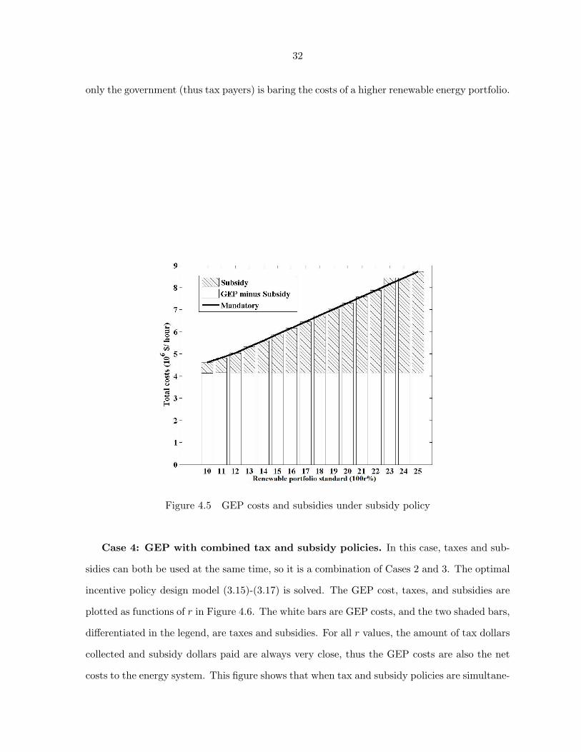
32

only the government (thus tax payers) is baring the costs of a higher renewable energy portfolio.

Figure 4.5 GEP costs and subsidies under subsidy policy

Case 4: GEP with combined tax and subsidy policies. In this case, taxes and sub-

sidies can both be used at the same time, so it is a combination of Cases 2 and 3. The optimal

incentive policy design model (3.15)-(3.17) is solved. The GEP cost, taxes, and subsidies are

plotted as functions of r in Figure 4.6. The white bars are GEP costs, and the two shaded bars,

differentiated in the legend, are taxes and subsidies. For all r values, the amount of tax dollars

collected and subsidy dollars paid are always very close, thus the GEP costs are also the net

costs to the energy system. This figure shows that when tax and subsidy policies are simultane-

33

ously imposed, they are much more efficient than either one type alone. The combined policies

require less taxes and less subsidies, and result in neutral government revenue. It is also worth

noting that the incentive policies are particularly efficient when the renewable portfolio goal is

below 17%; much more incentives would be needed to achieve a higher policy goal. Of course,

this threshold is dependent upon specific data being used, yet it demonstrates the capability of

our incentive policy design models to determine appropriate policy goals taking into account

the implications to the energy system. Compared to mandatory policy, the incentive policy

leads to similar net GEP costs, but it also provides a consistent penalty/incentive mechanism

to all power suppliers.

4.3.2 Sensitivity analysis of the policies

We also conduct sensitivity analysis on the efficiency of the policies with respect to coal

production costs increase, wind energy investment costs decrease, and transmission capacity

expansion.

As fossil fuel reserves become more and more depleted, the production cost can be expected

to have an increasing trend in the future. Figure 4.7 is the counterpart of Figure 4.6 with the

coal production costs being doubled. Although the GEP costs are almost doubled, the amount

of incentives required to achieve a same policy goal is only slightly reduced. This is because

wind operation cost is already lower than that of coal, whereas the wind capital investment

cost is the real bottleneck that needs to be overcome by policy intervention.

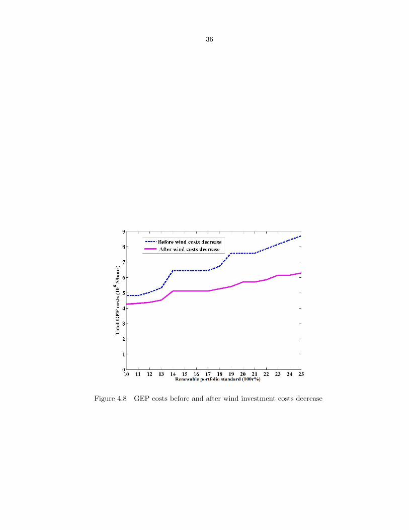
For the past decade, renewable energy techniques have made significant progress and the

investment costs continue to fall. Figures 4.8 and 4.9 compare the GEP costs and incentives,

respectively, before and after the wind investment costs are reduced by 50%. With such costs

decrease, not only the GEP costs are greatly reduced, it also requires much less incentives

to achieve a same policy goal. These results demonstrate the sensitivity of the efficiency of

34

Figure 4.6 GEP costs and incentives under tax-subsidy policy

incentive policies with respect to capital investment cost, which also validate the long-term

impact of incentive policies in promoting renewable energy.

Transmission capacity is another factor that could affect the effectiveness and efficiency

of policies. In many cases, inadequate transmission capacity is a bottleneck for remote and

windy areas to deliver wind power to load zones, thus building new transmission lines could

effectively increase renewable energy generation. However, we show an example in which the

removal of transmission lines would also increase the efficiency of incentive policies. We consider

our electricity transmission network with links 1-2 and 2-3 removed, which makes California

35

Figure 4.7 GEP costs before and after coal production costs increase

isolated from external supply of energy. Figures 4.10 and 4.11 compare the GEP costs and

incentives before and after the removal of the links. Without the two links, although the

GEP costs would be higher, it would actually require less incentives to achieve same renewable

portfolio goals. This is because wind would become a pivotal resource for electricity generation

when external supply becomes unavailable and local coal transportation has reached its limit.

Therefore, careful analysis is necessary to determine the actual effect of addition or removal of

transmission lines on renewable energy generation and policies.

36

Figure 4.8 GEP costs before and after wind investment costs decrease

37

Figure 4.9 Incentives costs before and after wind investment costs decrease

38

Figure 4.10 The total GEP costs in two situations

39

Figure 4.11 The total incentive costs in two situations

40

CHAPTER 5. CONCLUSION AND FUTURE WORK

5.1 Conclusion

We propose a bilevel optimization framework for designing effective and efficient incentive

policies to promote renewable energy in a generation capacity planning problem. The effective

of an incentive policy is its capability to achieve a goal that would not be achievable without

it, whereas the efficiency is defined as the amount of intervention, including tax collected,

subsidies paid, and GEP cost increase, to achieve the policy goal. The lower the intervention

to achieve a goal, the higher the efficiency.

Our analysis of the incentive policies, as well as the comparison with mandatory ones, are

in the context of generation expansion planning problem, in which the energy system makes

the investment decisions to meet projected demand. The objective of our proposed inverse

optimization model is to achieve a policy goal of renewable portfolio standard by promoting

more investment in renewable energy with a minimal amount of policy intervention.

An integrated energy system with a coal production/transportation network and an elec-

tricity generation/transmission network representing the contiguous United States is used for

a case study to demonstrate our approach. We gain the following insights from the results: (1)

incentive policies, if designed carefully with our proposed inverse optimization model, could

achieve the same policy goal as mandatory policies both effectively and efficiently; (2) com-

bining taxes and subsidies in an incentive policy is much more efficient than using either one

alone; (3) there could exist a policy threshold beyond which the efficiency of incentive policies

dramatically drops; (4) renewable investment costs decrease has a greater impact than non-

41

renewable generation costs increase on the efficiency of incentive policies; and (5) the addition

of transmission lines may or may not improve the efficiency of incentive policies.

5.2 Future Work

5.2.1 Future research on modeling

We will incorporate uncertainties about certain data parameters. The real circumstances in

the integrated energy system are however characterized by imperfect information about data,

namely electricity demands and fuel prices. A stochastic optimization problem formulation

would enable handling uncertain data.

5.2.2 Further improvement of algorithm and data

In this thesis, the incentive policy design model is solved by the heuristic algorithm. There

is no other heuristic algorithm for the policy design policy, we can’t compare the efficiency.

In the future study, we will conduct more research on further improvement of our heuristic

algorithm. By comparing the optimal solution, we can further study the efficiency of the

incentive policy design model. Moreover, the inverse optimization still needs more efficient

algorithm. In addition, We will improve data quality and quantity. Many of the assumptions

and modeling choices that have been made are the result of data limitations. A more complete

and accurate set of data would facilitate a more comprehensive analysis.

5.2.3 Writing an open source software

As far as we know, there is no software available for designing effective and efficient incentive

policies. We can write our algorithm into an open source software and publish it for researcher

or policy makers to design incentive policies.

42

BIBLIOGRAPHY

[1] World Energy Assessment 2004. [Online]. Available:

http://www.undp.org/energy/weaover2004.html.

[2] Energy Information Administration. [Online]. Available: http://www.eia.doe.gov.

[3] Nontechnical Barriers to Solar Energy Use: Review of Recent Literature. [Online]. Avail-

able: http://www.nrel.gov/docs/fy07osti/40116.pdf

[4] Gielecki, M., Mayes, F., Prete, L. (2000). Incentive, mandates, and government programs

for promoting renewable energies, renewable energy 2000: issues and trends. Technical

report, DOE/Energy Information Administration.

[5] Greenberg, H. J., Murphy, F. H. (1985). Computing market equilibria with price regula-

tions using mathematical programming. Operations Research, 33 (5), 935–954.

[6] Goulder, L. H.(1992). Carbon tax design and U.S. industry performance. Tax Policy and

the Economy, 6:59–104.

[7] Rader, N. A., Norgaard, R. B.(1996). Efficiency and sustainability in restructured elec-

tricity markets: the renewables portfolio standard. The Electricity Journal, 9 (6), 37–49.

[8] Solomon, B. D, Banerjee, A. (2006). A global survey of hydrogen energy research, develop-

ment and policy. Energy Policy, 34 (7), 781–792.

[9] Ahmed, S., King,A. J., Parija, G. (2003). A multi-stage stochastic integer programming

approach for capacity expansion under uncertainty. Journal of Global Optimization, 26,

3–24.

43

[10] Antunes, C. H., Martins, A. G., Brito, I. S.(2004). A multiple objective mixed integer

linear programming model for power generation expansion planning. Energy, 29, 613–627.

[11] Chuang, A. S., Wu, F., Varaiya, P.(2001). A game-theoretic model for generation expan-

sion planning: problem formulation and numerical comparisons. IEEE Transactions on

Power Systems, 16 (4), 885–891.

[12] Lopez,J. A., Ponnambalam, K., Quintana, V. H.(2009). Generation and transmission

expan- sion under risk using stochastic programming. IEEE Transactions on Power Sys-

tems, 22 (3), 1369–1378.

[13] Meza, J. L. C., Yildirim, M. B., Masud, A. S. M.(2007) . A model for the multiperiod multi-

objective power generation expansion problem. IEEE Transactions on Power Systems,

22 (2), 871–878.

[14] Mo, B., Hegge, J., Wangensteen, I.(1991). Stochastic generation expansion planning by

means of stochasticdynamic programming. IEEE Transactions on Power Systems, 6 (2),

662–668.

[15] Murphy, F. H., Smeers, Y.(2005). Generation capacity expansion in imperfectly compet-

itive restructured electricity markets. Operations Research, 53 (4), 646–661.

[16] States with Renewable Portfolio Standards. http://apps1.eere.energy.gov/states/maps/renewable

portfolio states.cfm.

[17] Berry, T., Jaccard, M.(2001). The renewable portfolio standard: design considerations

and an implementation survey. Energy Policy, 29, 263–277.

[18] Blok, K. (2006). Renewable energy policies in the European Union. Energy Policy, 34,

251–255.

[19] Chupka, M. W.(2003). Designing effective renewable markets. The Electricity Journal,

16 (4), 46–57.

44

[20] Mitchell, C., Bauknecht, D., Connor. P. M. (2006). Effectiveness through risk reduction:

a comparison of the renewable obligation in england and wales and the feed-in system in

Germany. Energy Policy, 24, 297–305.

[21] Palmer, K., Burtraw, D. (2005). Cost-effectiveness of renewable electricity policies. Energy

Economics, 27, 873–894.

[22] Bloom, J.(1982). Long-range generation planning using decomposition and probabilistic

simu- lation. IEEE Transactions on Power Apparatus and Systems, 101 (4), 797–802.

[23] Loiter, J. M., Norberg-Bohm, V.(1999). Technology policy and renewable energy: public

roles in the development of new energy technologies. Energy Policy, 27, 85–97.

[24] Roy, B., Kerry, K., Kip, V. W. (1995). Energy Taxation as a policy instrument to Re-

duce CO2 Emissions: A Net Benefit Analysis Journal of Environmental Economics and

Management 29 (1), 1–24.

[25] Majumdar, S., Chattopadhyay, D.(1999). A model for integrated analysis of generation

capacity expansion and financial planning. IEEE Transactions on Power Systems, 14 (2),

466–471.

[26] Nemet, G.F., Baker, E. (2009) Demand subsidies versus R&D: comparing the uncertain

impacts of policy on a pre-commercial low-carbon energy technology, The Energy Journal,

30 (4), 873–894.

[27] Duan, Z., Wang, L.(2010). Parallel algorithms for the inverse mixed integer linear program-

ming problem. Under review.

[28] Wang, L.(2009). Cutting plane algorithms for the inverse mixed integer linear program-

ming problem. Operations Research Letters, 37 (2), 114–117.

[29] Zhou, Y, Wang, L, McCalley, J. D.(2010). Effective incentives design for renewable energy

generation expansion planning: An inverse optimization approach. Proceedings of the

IEEE PES General Meeting, 2010.

45

[30] Menke, W.(1989). Geophysical data analysis: discrete inverse theory. Academic Press, San

Diego.

[31] Zhang, J., Liu, Z.(1996). Calculating some inverse linear programming problem. Journal

of Computational and Applied Mathematics, 72, 261–273.

[32] Yang, C., Zhang, J.(1997). Inverse maximum flow and minimum cut problems. Optimiza-

tion, 40, 147–170.

[33] Zhang, J., Liu, Z., Ma, Z.(1996). On inverse problem of minimum spanning tree with

partition constraints. ZOR-Mathematical Methods of Operations Research, 44, 347–358.

[34] Hu, Z., Liu, Z.(1998). A strongly polynomial algorithm for the inverse arborescence prob-

lem. Discrete Applied Mathematics, 82, 135–154.

[35] Ahuja, R. K., Orlin, J. B.(2001). Inverse optimization. Operations Research, 49 (5), 771–

783, 2001.

[36] Zhang, Z.(1999). Solution Structure of Some Inverse Combinatorial Optimization Prob-

lems. Journal of Combinatorial Optimization , 3, 127–139.

[37] Heuberger, C. (2004). Inverse combinatorial optimization: a survey on problems, methods,

and results. Journal of Combinatorial Optimization, 8, 329–361.

[38] Energy Information Administration, Annual Coal Report 2002, DOE/EIA-0584 (2002),

Washington, DC, 2003.

[39] Energy Information Administration, Annual Energy Outlook 2005, DOE/EIA-0383 (2005),

Washington, DC, February 2005.

[40] Energy Information Administration, Annual Energy Review 2002, DOE/EIA-0384 (2002),

Washington, DC, October 2003.

[41] Quelhas, A.(2006). Economic effciency of the energy ows from the primary resource sup-

pliers to the electric load centers. Ph.D. dissertation, Iowa State University, 2006.

46

[42] DOE EIA Report: DOE/EIA-0554, June 2008 on Generation Technologies Cost. [Online].

Available: http:// www.eia.doe.gov/fuelelectric.html.