Designing an optimal connected nature reserve

Applied Mathematical Modelling 36 (2012) 2213–2223

Contents lists available at SciVerse ScienceDirect

Applied Mathematical Modelling

journal homepage: www.elsevier .com/locate /apm

Designing an optimal connected nature reserve

Alain Billionnet ⇑Laboratoire CEDRIC, Ecole Nationale Supérieure d’Informatique pour l’Industrie et l’Entreprise, 1, square de la résistance, 91025 Evry cedex, France

a r t i c l e i n f o

Article history:Received 18 December 2010Received in revised form 21 July 2011Accepted 9 August 2011Available online 18 August 2011

Keywords:Conservation planningSpatial considerationsConnected networkInteger programming

0307-904X/$ - see front matter � 2011 Elsevier Incdoi:10.1016/j.apm.2011.08.002

⇑ Tel.: +33 1 69 36 73 33; fax: +33 1 69 36 73 05E-mail address: [email protected]

a b s t r a c t

We consider a landscape divided into elementary cells, each of these cells containing somespecies to be protected. We search to select a set of cells to form a natural reserve in orderto protect all the species present in the landscape. A species is considered protected if it ispresent in a certain number of cells of the reserve. There is an important spatial constraintconcerning the set of selected cells: a species must be able to go from any cell to any cellwithout leaving the reserve. An integer linear programming model was proposed by Önaland Briers [2] for this reserve selection problem, but the size of the problems which can behandled by this model is limited: several hours of computation are required for solvinginstances with hundred of cells and hundred of species. Having proposed an improvementof this model which reduces appreciably the computation time, we propose anotherinteger linear programming model, easy to carry out, which allows to obtain, in a few sec-onds of computation, optimal or near-optimal solutions for instances with hundred of cellsand hundred of species. However, the computation time becomes prohibitive for instanceswith more than 200 cells and 100 species. But, this approach can be particularly useful tosolve the problem, in an approximate way, by aggregation of cells as proposed by Önal andBriers [2].

� 2011 Elsevier Inc. All rights reserved.

1. Introduction

The increase of the human population and the development of its activities result in dramatic habitat loss for numerousspecies with, as a consequence, a decline of the biodiversity. The creation of protected areas is the main tool for species pres-ervation but the available means to protect these zones are obviously limited. It is thus important to select them efficiently.The problem was studied a lot, and numerous publications are available in the biological conservation literature (see, forexample [1]). In this article, we are concerned with completely connected reserves. In such reserves, the species can movefrom any site to any site without leaving the reserve. The reader may refer to the article by Önal and Briers [2] for a detaileddiscussion of the relevance of such reserves. As mentioned by these authors, to define a connected reserve of minimal sizeand allowing to protect a predefined set of species is a complex combinatorial optimization problem. They formulate theproblem by an integer linear program and present some computational experiments showing that only small-sized instancescan be solved by this program. We propose here a slight improvement of this model, inspired by a well known formulationfor the classical traveling salesman problem. This formulation allows the solution of the reserve selection problem to bestrongly accelerated in comparison with the formulation proposed by Önal and Briers [2], but does not allow to handleinstances of significantly larger size. We also propose another simple integer linear programming model which allows toquickly obtain optimal or near-optimal solutions for medium-sized instances. This heuristics approach is particularly easyto implement because it uses only standard integer linear programming software. It allows to obtain, in a few seconds of

. All rights reserved.

.

http://dx.doi.org/10.1016/j.apm.2011.08.002

mailto:[email protected]

http://dx.doi.org/10.1016/j.apm.2011.08.002

http://www.sciencedirect.com/science/journal/0307904X

http://www.elsevier.com/locate/apm

2214 A. Billionnet / Applied Mathematical Modelling 36 (2012) 2213–2223

computation, optimal or near-optimal solutions for instances containing hundred of cells and hundred of species. However,when the instances contain more than 200 cells and 100 species, the computation time becomes prohibitive. But, this ap-proach can be very useful to solve the problem, in an approximate way, by aggregation of cells as proposed by Önal andBriers [2].

2. The problem

Let S = {s1,s2, . . . ,sp} be the set of species concerned by the study. To simplify the presentation, we suppose, in a classicway, that the studied zone is represented by a matrix C of m � n square cells. For every cell cij of this matrix, we knowthe species present in this cell. More exactly, the Boolean parameter aijk is equal to 1 if and only if the species sk is presentin the cell cij. Two cells are considered as adjacent if they share a common side. Furthermore, we denote by bk the number ofcells of the matrix C where the species sk is present. We thus try to select a minimal number of cells such that:

1. Every species sk (k = 1, . . . ,p) is present in at least ek (ek P 1) of the selected cells (only in bk cells if bk < ek). In other words,the species sk must be present in at least min(ek,bk) cells of the reserve.

2. There is a possible movement from any cell of the reserve to any cell of the reserve without leaving the reserve, and ingoing progressively from a cell to an adjacent cell.

2.1. Graph formulation

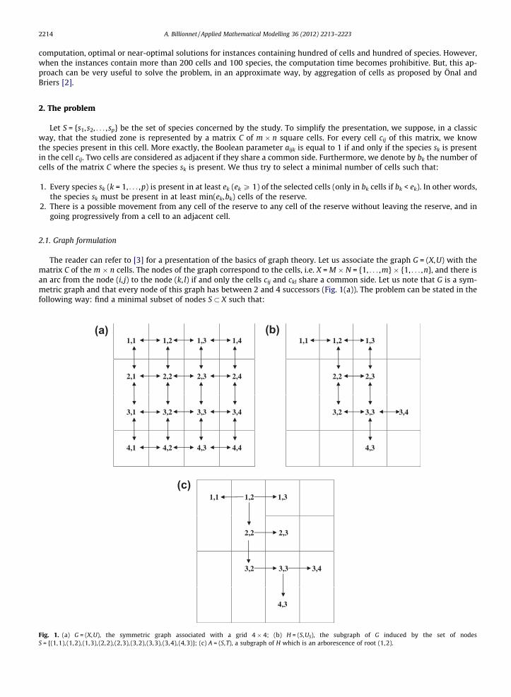
The reader can refer to [3] for a presentation of the basics of graph theory. Let us associate the graph G = (X,U) with thematrix C of the m � n cells. The nodes of the graph correspond to the cells, i.e. X = M � N = {1, . . . ,m} � {1, . . . ,n}, and there isan arc from the node (i, j) to the node (k, l) if and only the cells cij and ckl share a common side. Let us note that G is a sym-metric graph and that every node of this graph has between 2 and 4 successors (Fig. 1(a)). The problem can be stated in thefollowing way: find a minimal subset of nodes S � X such that:

1,1 1,2 1,3 1,4 1,1 1,2 1,3

2,1 2,2 2,3 2,4 2,2 2,3

3,1 3,2 3,3 3,4 3,2 3,3 3,4

4,1 4,2 4,3 4,4 4,3

1,1 1,2 1,3

2,2 2,3

3,2 3,3 3,4

4,3

(a) (b)

(c)

Fig. 1. (a) G = (X,U), the symmetric graph associated with a grid 4 � 4; (b) H = (S,US), the subgraph of G induced by the set of nodesS = {(1,1), (1,2), (1,3), (2,2), (2,3), (3,2), (3,3), (3,4), (4,3)}; (c) A = (S,T), a subgraph of H which is an arborescence of root (1,2).

A. Billionnet / Applied Mathematical Modelling 36 (2012) 2213–2223 2215

1. Every species sk is present in at least min(ek,bk) nodes of S.2. The subgraph induced by S is connected (Fig. 1(b)) or, equivalently, for each couple of nodes (x,y) of S, there exits a path of

G from x to y using only nodes of S.

The point 2 can be also stated as follows: the subgraph of G induced by the set of nodes S contains an arborescence, i.e. agraph A = (S,T) satisfying the following properties (Fig. 1(c)):

1. Each node of A has at most one direct predecessor.2. The number of arcs in A is equal to jSj � 1.3. A does not contains circuits.

3. Modeling the problem by integer linear programming

Integer linear programming is a classical tool in operations research that can be applied to a lot of optimization problems.The technique is known and well-tried but must be carefully implemented since some formulations may require a prohib-itive computation time (see, for example [4,5]). Indeed, several models are often possible for the same problem, and thechoice of a good one is particularly important. First of all, we recall in this section the integer linear programming modelproposed by Önal and Briers [2], and then we propose a slight improvement of this model. This improvement concernsthe modeling, by integer linear programming, of the search, in a graph, for a subset of arcs which does not contain circuits.This modeling is inspired by a classic model for the famous traveling salesman problem (see, for example [6]).

3.1. Model 1 [2]

Let us remind that we search for a subset of cells satisfying some properties as regard to the species present in these cells,and such that the subgraph induced by these cells contains an arborescence. There are two types of variables in this model:the Boolean variables xij which are equal to 1 if and only if the node (i, j) is selected, and the Boolean variables yijkl which areequal to 1 if and only if the arc ((i, j), (k, l)), i.e. the arc going from (i, j) to (k, l), is retained to form the arborescence. The mixed-integer linear program (P1) is proposed by Önal and Briers [2].

ðP1Þ minX

ði;jÞ2M�N

xij

s:t:Xm

i¼1

Xn

j¼1

aijkxij P minðek; bkÞ k ¼ 1; . . . ; p; ð1:1ÞX

ðk;lÞ2Aþij

yijkl 6 4xij ði; jÞ 2 M � N; ð1:2Þ

X

ði;jÞ2A�kl

yijkl 6 xkl ðk; lÞ 2 M � N; ð1:3Þ

X

ðði;jÞ;ðk;lÞÞ2U

yijkl ¼X

ði;jÞ2M�N

xij � 1; ð1:4Þ

zijkl P wij þ 1� Pð1� yijklÞ ðði; jÞ; ðk; lÞÞ 2 U; ð1:5Þwkl ¼

X

ði;jÞ2A�kl

zijkl ðk; lÞ 2 M � N; ð1:6Þ

zijkl P 0; yijkl 2 f0;1g ðði; jÞ; ðk; lÞÞ 2 U; ð1:7Þxij 2 f0;1g ði; jÞ 2 M � N: ð1:8Þ

Recall that U is the set of arcs of the graph associated with the grid. For all ði; jÞ 2 M � N ¼ f1; . . . ;mg � f1; . . . ;ng; Aþij is theset of nodes successors of the node (i, j) and A�ij is the set of nodes predecessors of the node (i, j). In other words,Aþij ¼ ðk; lÞ 2 X : ðði; jÞ; ðk; lÞÞ 2 Uf g and A�ij ¼ ðk; lÞ 2 X : ððk; lÞ; ði; jÞÞ 2 Uf g. P is a sufficiently large constant (an upper boundof the number of cells in an optimal reserve). The objective function expresses the number of cells selected to form the re-serve. The constraint (1.1) expresses the fact that each species must be present in at least min(ek,bk) cells of the reserve. Gi-ven a subset S of nodes and x its characteristic vector, a vector y of RjUj defines an arborescence on the subgraph induced by Sif and only if the constraints (1.2)–(1.8) are satisfied. The constraint (1.2) imposes that, if a node is not selected, then thenumber of retained arcs of which this node is the initial extremity is equal to 0. In the contrary case, this constraint playsno role because, in a graph associated with a grid, the number of arcs leaving each node is less than or equal to 4. The con-straint (1.3) expresses that if the node (k, l) is not retained then no arcs ending in (k, l) can be retained. Should the oppositeoccur, at most one arc ending in (k, l) can be retained. The constraint (1.4) imposes that the number of retained arcs is equalto the number of selected nodes minus one. The constraints (1.5)–(1.7) where P is a sufficiently large constant, eliminate thepossibility of cycle formation [2]. Let us note that it would be easy in such a model to take into account the acquisition costsof the cells. Let us suppose that the cost of the cell cij is equal to dij. This cost can be taken into account in the objective


function by searching for a reserve of minimal cost and satisfying the constraints. The objective function to be minimizedwould be then

Pði;jÞ2M�Ndijxij. We can also take into account these costs by introducing a budgetary constraintP

ði;jÞ2M�Ndijxij 6 B, where B is the available budget.

3.2. An improvement of Model 1: Model 2

This improvement concerns the constraints of (P1) defining an arborescence, that is the constraints (1.2)–(1.8). We keepthe constraints (1.3), (1.4) and (1.8), we replace the constraint (1.2) by yijkl 6 xij ((i, j), (k, l)) 2 U, and we replace the constraintswhich forbid circuits, that is constraints (1.5)–(1.7), by the constraints tkl P tij + 1 � P(1 � yijkl) for every arc ((i, j), (k, l)) of U;tij P 0 is a real variable associated with each node (i, j). So, we obtain the mixed-integer linear program (P2).

ðP2Þ minX

ði;jÞ2M�N

xij

s:t:Xm

i¼1

Xn

j¼1

aijkxij P minðek; bkÞ k ¼ 1; . . . ; p; ð2:1Þ

yijkl 6 xij ðði; jÞ; ðk; lÞÞ 2 U; ð2:2ÞX

ði;jÞ2A�kl

yijkl 6 xkl ðk; lÞ 2 M � N; ð2:3Þ

X

ðði;jÞ;ðk;lÞÞ2U

yijkl ¼X

ði;jÞ2M�N

xij � 1; ð2:4Þ

tkl P tij þ 1� Pð1� yijklÞ ðði; jÞ; ðk; lÞÞ 2 U; ð2:5Þtij P 0; xij 2 f0;1g ði; jÞ 2 M � N; ð2:6Þyijkl 2 f0;1g ðði; jÞ; ðk; lÞÞ 2 U: ð2:7Þ

The constraints (2.2)–(2.5), together with the constraints (2.6) and (2.7) which specify the nature of the variables, impose toretain a set of nodes and a set of arcs forming an arborescence. The constraint (2.2) imposes that the arc ((i, j), (k, l)) cannot beretained if the node (i, j) corresponding to the initial extremity of this arc is not retained. The constraint (2.3) is identical tothe constraint (1.3). Finally, the constraint (2.5) forbids that a circuit be formed by the retained arcs. This set of constraints,where P is a sufficiently large constant, is similar to those which are used in some formulations of the traveling salesmanproblem to eliminate sub-tours by using a polynomial number of constraints (see, for example [6]). A nonnegative valuetij is assigned to each node (i, j) of the graph and, if the arc ((i, j), (k, l)) is retained (yijkl = 1) then tkl must be greater than orequal to tij + 1. So, the set of retained arcs cannot form a circuit. If the arc ((i, j), (k, l)) is not retained (yijkl = 0) then the con-straints (2.5) is always satisfied (if the values of tij are less than or equal to P � 1). Note that the summation over (k, l) is pos-sible in constraint (2.2). This gives the constraint (1.2). This replacement of (2.2) by (1.2) reduces the total number ofconstraints but deteriorates slightly the optimal value of the continuous relaxation of (P2). Computational experiments haveshown that (2.2) was more efficient than (1.2). Models 1 and 2 are presented for a land area represented by a matrix of m � nsquare cells but they could be easily extended to a land area divided into an arbitrary set of cells.

4. Models 1 and 2: computational experiments

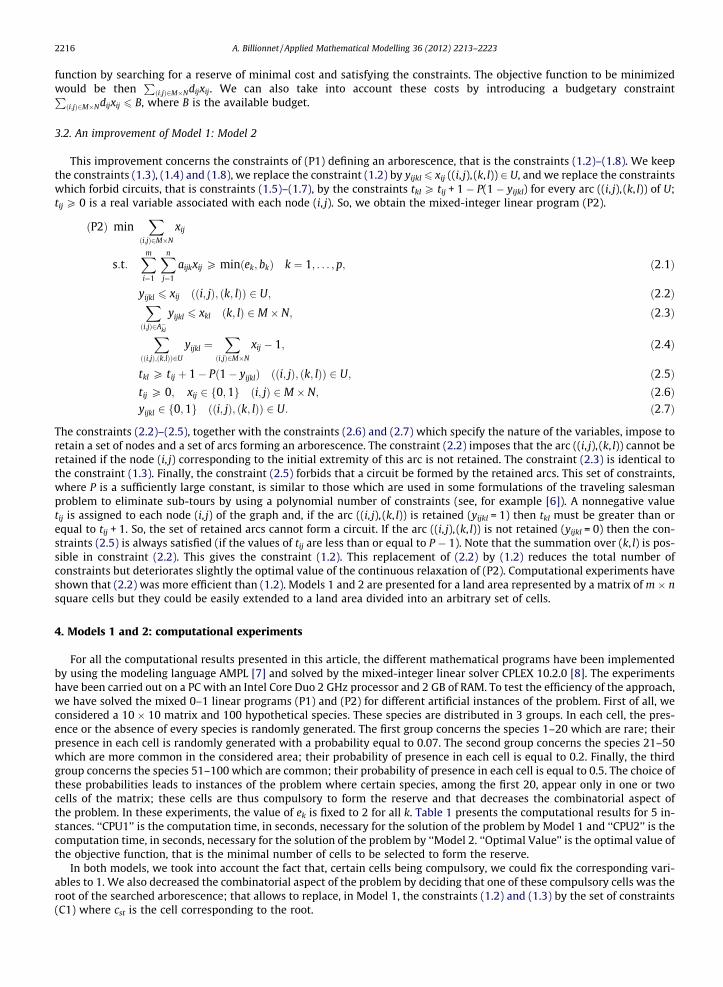
For all the computational results presented in this article, the different mathematical programs have been implementedby using the modeling language AMPL [7] and solved by the mixed-integer linear solver CPLEX 10.2.0 [8]. The experimentshave been carried out on a PC with an Intel Core Duo 2 GHz processor and 2 GB of RAM. To test the efficiency of the approach,we have solved the mixed 0–1 linear programs (P1) and (P2) for different artificial instances of the problem. First of all, weconsidered a 10 � 10 matrix and 100 hypothetical species. These species are distributed in 3 groups. In each cell, the pres-ence or the absence of every species is randomly generated. The first group concerns the species 1–20 which are rare; theirpresence in each cell is randomly generated with a probability equal to 0.07. The second group concerns the species 21–50which are more common in the considered area; their probability of presence in each cell is equal to 0.2. Finally, the thirdgroup concerns the species 51–100 which are common; their probability of presence in each cell is equal to 0.5. The choice ofthese probabilities leads to instances of the problem where certain species, among the first 20, appear only in one or twocells of the matrix; these cells are thus compulsory to form the reserve and that decreases the combinatorial aspect ofthe problem. In these experiments, the value of ek is fixed to 2 for all k. Table 1 presents the computational results for 5 in-stances. ‘‘CPU1’’ is the computation time, in seconds, necessary for the solution of the problem by Model 1 and ‘‘CPU2’’ is thecomputation time, in seconds, necessary for the solution of the problem by ‘‘Model 2. ‘‘Optimal Value’’ is the optimal value ofthe objective function, that is the minimal number of cells to be selected to form the reserve.

In both models, we took into account the fact that, certain cells being compulsory, we could fix the corresponding vari-ables to 1. We also decreased the combinatorial aspect of the problem by deciding that one of these compulsory cells was theroot of the searched arborescence; that allows to replace, in Model 1, the constraints (1.2) and (1.3) by the set of constraints(C1) where cst is the cell corresponding to the root.

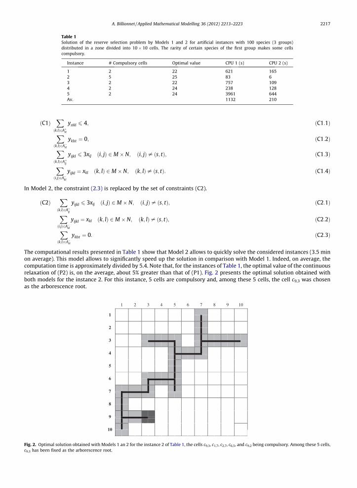
Table 1Solution of the reserve selection problem by Models 1 and 2 for artificial instances with 100 species (3 groups)distributed in a zone divided into 10 � 10 cells. The rarity of certain species of the first group makes some cellscompulsory.

Instance # Compulsory cells Optimal value CPU 1 (s) CPU 2 (s)

1 2 22 621 1652 5 25 83 63 2 22 757 1094 2 24 238 1285 2 24 3961 644Av. 1132 210

Fig. 2.c9,3 has


ðC1ÞX

ðk;lÞ2Aþst

ystkl 6 4; ðC1:1Þ

X

ðk;lÞ2A�st

yklst ¼ 0; ðC1:2Þ

X

ðk;lÞ2Aþij

yijkl 6 3xij ði; jÞ 2 M � N; ði; jÞ– ðs; tÞ; ðC1:3Þ

X

ði;jÞ2A�kl

yijkl ¼ xkl ðk; lÞ 2 M � N; ðk; lÞ – ðs; tÞ: ðC1:4Þ

In Model 2, the constraint (2.3) is replaced by the set of constraints (C2).

ðC2ÞX

ðk;lÞ2Aþij

yijkl 6 3xij ði; jÞ 2 M � N; ði; jÞ– ðs; tÞ; ðC2:1Þ

X

ði;jÞ2A�kl

yijkl ¼ xkl ðk; lÞ 2 M � N; ðk; lÞ– ðs; tÞ; ðC2:2Þ

X

ðk;lÞ2A�st

yklst ¼ 0: ðC2:3Þ

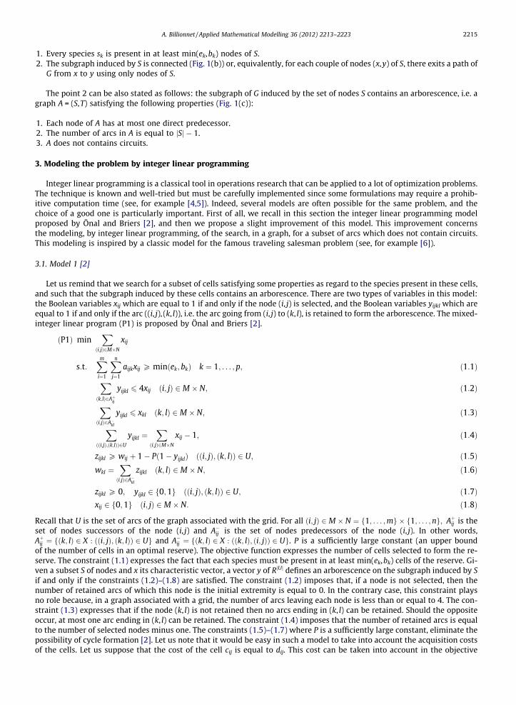
The computational results presented in Table 1 show that Model 2 allows to quickly solve the considered instances (3.5 minon average). This model allows to significantly speed up the solution in comparison with Model 1. Indeed, on average, thecomputation time is approximately divided by 5.4. Note that, for the instances of Table 1, the optimal value of the continuousrelaxation of (P2) is, on the average, about 5% greater than that of (P1). Fig. 2 presents the optimal solution obtained withboth models for the instance 2. For this instance, 5 cells are compulsory and, among these 5 cells, the cell c9,3 was chosenas the arborescence root.

Optimal solution obtained with Models 1 an 2 for the instance 2 of Table 1, the cells c9,3, c1,7, c2,7, c6,5, and c9,2 being compulsory. Among these 5 cells,been fixed as the arborescence root.

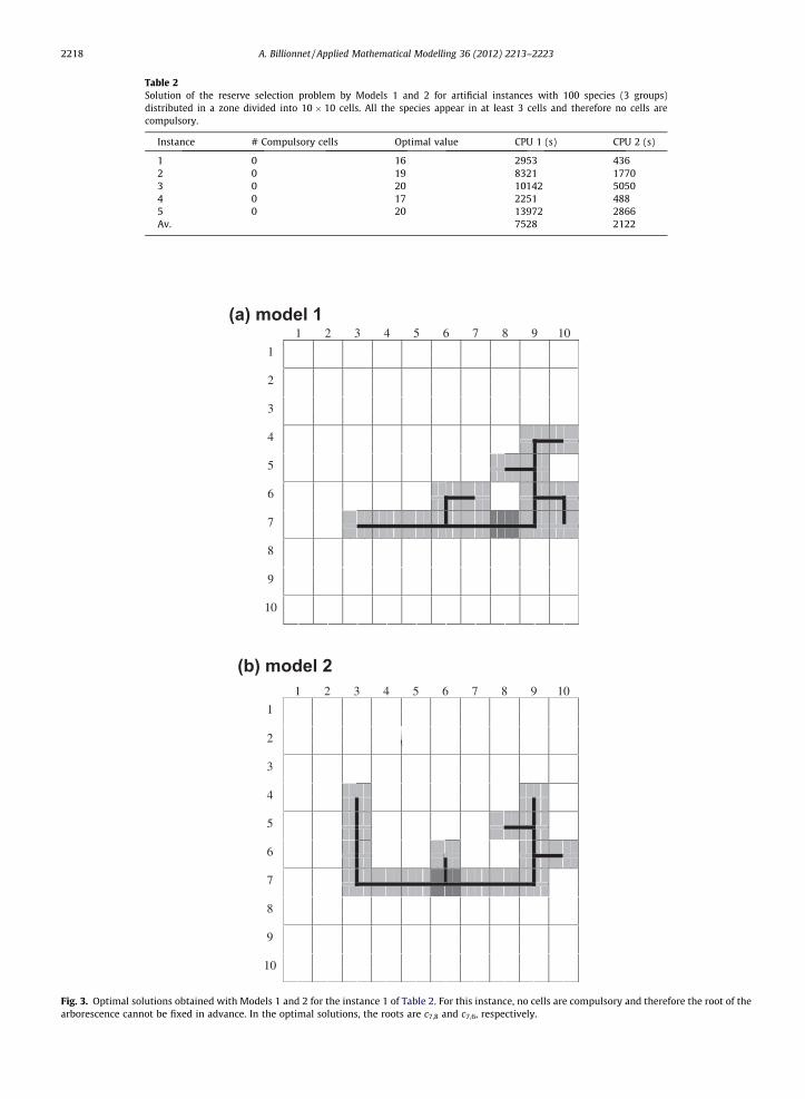
Table 2Solution of the reserve selection problem by Models 1 and 2 for artificial instances with 100 species (3 groups)distributed in a zone divided into 10 � 10 cells. All the species appear in at least 3 cells and therefore no cells arecompulsory.

Instance # Compulsory cells Optimal value CPU 1 (s) CPU 2 (s)

1 0 16 2953 4362 0 19 8321 17703 0 20 10142 50504 0 17 2251 4885 0 20 13972 2866Av. 7528 2122

1 2 3 4 5 6 7 8 9 10

1

2

3

4

5

6

7

8

9

10

1 2 3 4 5 6 7 8 9 10

1

2

3

4

5

6

7

8

9

10

(b) model 2

(a) model 1

Fig. 3. Optimal solutions obtained with Models 1 and 2 for the instance 1 of Table 2. For this instance, no cells are compulsory and therefore the root of thearborescence cannot be fixed in advance. In the optimal solutions, the roots are c7,8 and c7,6, respectively.



In the second series of experiments we kept a 10 � 10 matrix and 100 hypothetical species but, to generate instances, wemodified the probabilities of presence of the different species in each cell so that no cell is compulsory. It means that everyspecies appears in at least 3 cells of the matrix. In these experiments, the species are always distributed in 3 groups. The firstgroup concerns the species 1–20, the probability of presence of which in each cell is equal to 0.1. The second group concernsthe species 21–50, the probability of presence of which in each cell is equal to 0.2. Finally, the third group concerns the spe-cies 51–100, the probability of presence of which in each cell is equal to 0.5. Table 2 presents the computational results forModel 1 and Model 2 for 5 instances. These computational results show that Models 1 and 2 allow to solve the consideredinstances. However, computation times are much more important (approximately 125 min and 35 min on average, respec-tively) than in the case where some cells are compulsory (Table 1). The results of Table 2 also show that Model 2 allows tosignificantly speed up the solution in comparison with Model 1. Indeed, on average, the computation time is approximatelydivided by 3.5. Note that, for the instances of Table 2, the optimal value of the continuous relaxation of (P2) is, on the average,about 3% greater than that of (P1). The Fig. 3 presents the optimal solutions obtained with Models 1 and 2 for the instance 1of Table 2.

As mentioned at the beginning of this section, the computational experiments were carried out with the AMPL modelinglanguage coupled with the solver CPLEX. To confirm the results presented in Tables 1 and 2 and showing the efficiency ofModel 2, we have conducted some computational experiments with another linear programming tool: the MPL modelinglanguage coupled with the XA solver [9]. The XA solver is much less efficient than the CPLEX solver, but it allowed us tocompare solution times of Models 1 and 2. For 10 instances randomly generated, with 8 � 8 cells, 50 species and nomandatory cells, none has been solved by Model 1 in less than 1800 s of computation time. In contrast, all these instanceshave been solved by Model 2 within this time limit with an average computing time of 209 s. The efficiency of Model 1 overModel 2 can be explained by two factors. First, in Model 1, mn variables wij, 4mn-2m-2n variables zijkl, and 5mn-2m-2n con-straints are used to prohibit the circuits while, in Model 2, mn variables tij and 4mn-2m-2n constraints are sufficient. Then, inall the experiments we conducted, the optimal value of the continuous relaxation of Model 2 is slightly higher than theoptimum value of the continuous relaxation of Model 1. For the 10 instances mentioned above, the average improvementis of about 4%.

5. A new model: Model 3

In this section, we present a formulation of the problem, always by integer linear programming, but a little more restric-tive. The experiments carried out on this formulation show that it often allows to obtain very quickly an optimal solution ofthe problem (at least in our experimental conditions). Let us note however that the solution obtained by this model can benon-optimal. So, Model 3 can be used to solve large problems by an approach consisting of the aggregation of cells as it isproposed by Önal and Briers [2]. Indeed with this model, the solution of every sub-problem is quickly obtained, what is notthe case with the model proposed by these authors (Model 1). Model 3 differs from Model 2 by the constraints forbidding thecircuits. In Model 2, constraints (2.5) prevent the retained arcs to form a circuit. It is known that these type of constraints is

1 2 3 4 5 6 7 8 9 10

1

2

3

4

5

6

7

8

9

10

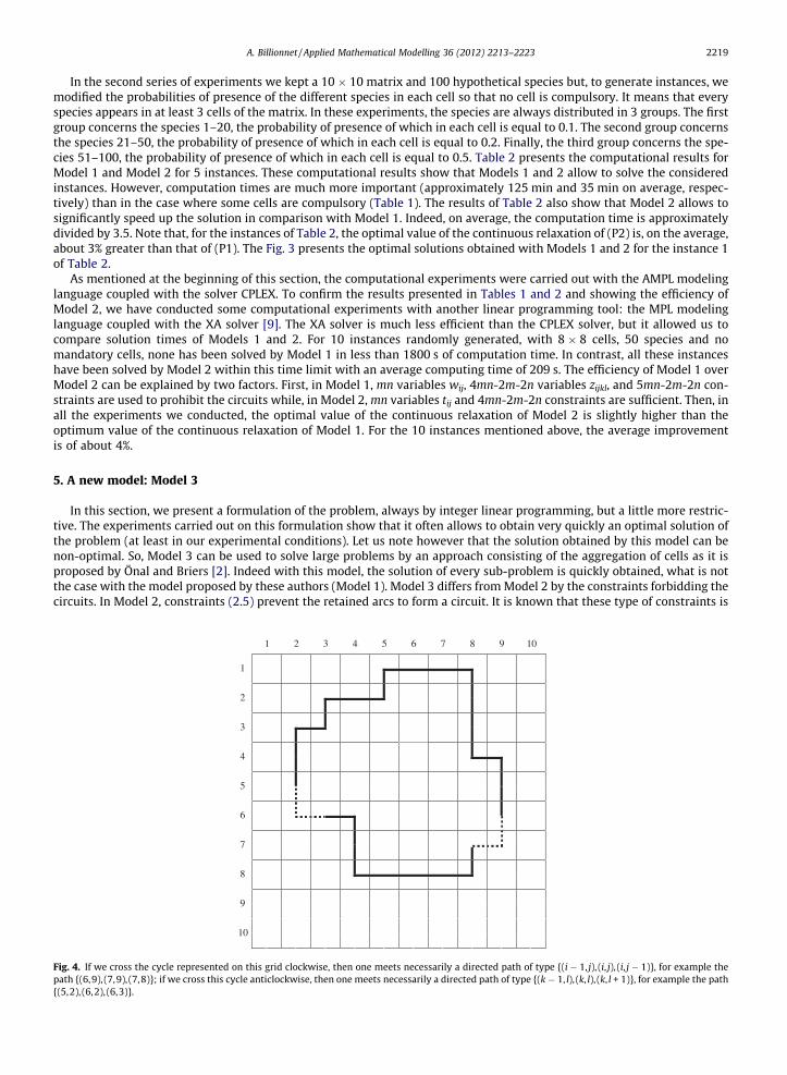
Fig. 4. If we cross the cycle represented on this grid clockwise, then one meets necessarily a directed path of type {(i � 1, j), (i, j), (i, j � 1)}, for example thepath {(6,9), (7,9), (7,8)}; if we cross this cycle anticlockwise, then one meets necessarily a directed path of type {(k � 1, l), (k, l), (k, l + 1)}, for example the path{(5,2), (6,2), (6,3)}.

),1( ji −↓

)1,( −ji ← ),( ji

),1( ji −↓

),( ji → )1,( +ji

Fig. 5. These two types of directed path of length 2 are forbidden by constraints (C3.2) and (C3.3).


not very effective, for example for the traveling salesman problem. We are going to replace them by other constraints. First ofall, we introduce the classic constraints forbidding the circuits of length 2, then constraints specific to the considered graph –associated with a grid – and based on the following idea: so that the arborescence solution does not contain circuits, it isenough to forbid, besides the circuits of length 2, the directed paths of two arcs and of type {(i � 1, j), (i, j), (i, j � 1)} or{(i � 1, j), (i, j), (i, j + 1)}. If the first type of path is forbidden, we cannot retain clockwise circuits of length greater than 2,and, if the second type of path is forbidden, we cannot retain anticlockwise circuits of length greater than 2 (Fig. 4).Wecan now express Model 3 from Model 2 by replacing the constraint (2.5) and the constraint tij P 0 by the three constraints(C3).

ðC3Þ yijkl þ yklij 6 1 ðði; jÞ; ðk; lÞÞ 2 U; k > i or l > j; ðC3:1Þyi�1;j;i;j þ yi;j;i;j�1 6 1 ði; jÞ 2 M � N; i P 2; j P 2; ðC3:2Þyi�1;j;i;j þ yi;j;i;jþ1 6 1 ði; jÞ 2 M � N; i P 2; j 6 n� 1: ðC3:3Þ

Let (P3) be the corresponding mathematical program. The constraint (C3.1) forbids the circuits of length 2. The constraints(C3.2) and (C3.3), by forbidding certain directed paths of length 2, forbid the circuits of length greater than 2. The variables tij

((i, j) 2M � N) of (P2) do not appear any more in (P3). Note that the reserves shown in Fig. 3 can be obtained by Model 3.Indeed, constraints (C3.2) and (C3.3) eliminate the directed paths of length 2 presented in Fig. 5. It is clear that both rootedtrees of Fig. 3 do not contain these types of directed path.

6. Experiments on Model 3

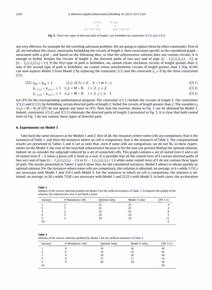
Take back the same instances as for Models 1 and 2: first of all, the instances where some cells are compulsory, that is theinstances of Table 1, and then the instances where no cell is compulsory, that is the instances of Table 2. The computationalresults are presented in Tables 3 and 4. Let us note that, even if some cells are compulsory, we do not fix, in these experi-ments on the Model 3, the root of the searched arborescence because to fix the root can prevent finding the optimal solution.Indeed, let us consider the subgraph induced by a set of connected cells. This graph contains a set of rooted trees E and a setof rooted trees E � E when a given cell is fixed as a root. It is possible that all the rooted trees of E contain directed paths oftwo arcs and of type {(i � 1, j), (i, j), (i, j � 1)} or {(i � 1, j), (i, j), (i, j + 1)} while some rooted trees of E do not contain these typesof path. The results presented in Tables 3 and 4 show that, for the considered instances, Model 3 allows to obtain quickly anoptimal solution. For the instances where some cells are compulsory, this solution is obtained, on average, in 6 s while 1132 sare necessary with Model 1 and 210 s with Model 2. For the instances in which no cell is compulsory, the solution is ob-tained, on average, in 26 s while 7528 s are necessary with Model 1 and 2122 s with Model 2. In both cases, the acceleration

Table 3Solution of the reserve selection problem by Model 3 for the artificial instances of Table 1. To improve the quality of thesolution, the arborescence root is not fixed a priori.

Instance # Mandatory cells Optimal value Model 3 value CPU 3 (s)

1 2 22 22 42 5 25 25 23 2 22 22 84 2 24 24 35 2 24 24 13Av. 6

Table 4Solution of the reserve selection problem by Model 3 for the artificial instances of Table 2.

Instance # Mandatory cells Optimal value Model 3 value CPU 3 (s)

1 0 16 16 102 0 19 19 453 0 20 20 394 0 17 17 145 0 20 20 20Av. 26

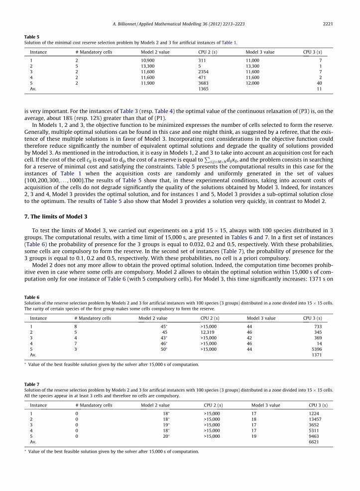
Table 5Solution of the minimal cost reserve selection problem by Models 2 and 3 for artificial instances of Table 1.

Instance # Mandatory cells Model 2 value CPU 2 (s) Model 3 value CPU 3 (s)

1 2 10,900 311 11,000 72 5 13,300 5 13,300 13 2 11,600 2354 11,600 74 2 11,600 471 11,600 25 2 11,900 3683 12,000 40Av. 1365 11


is very important. For the instances of Table 3 (resp. Table 4) the optimal value of the continuous relaxation of (P3) is, on theaverage, about 18% (resp. 12%) greater than that of (P1).

In Models 1, 2 and 3, the objective function to be minimized expresses the number of cells selected to form the reserve.Generally, multiple optimal solutions can be found in this case and one might think, as suggested by a referee, that the exis-tence of these multiple solutions is in favor of Model 3. Incorporating cost considerations in the objective function couldtherefore reduce significantly the number of equivalent optimal solutions and degrade the quality of solutions providedby Model 3. As mentioned in the introduction, it is easy in Models 1, 2 and 3 to take into account an acquisition cost for eachcell. If the cost of the cell cij is equal to dij, the cost of a reserve is equal to

Pði;jÞ2M�Ndijxij, and the problem consists in searching

for a reserve of minimal cost and satisfying the constraints. Table 5 presents the computational results in this case for theinstances of Table 1 when the acquisition costs are randomly and uniformly generated in the set of values{100,200,300, . . . ,1000}.The results of Table 5 show that, in these experimental conditions, taking into account costs ofacquisition of the cells do not degrade significantly the quality of the solutions obtained by Model 3. Indeed, for instances2, 3 and 4, Model 3 provides the optimal solution, and for instances 1 and 5, Model 3 provides a sub-optimal solution closeto the optimum. The results of Table 5 also show that Model 3 provides a solution very quickly, in contrast to Model 2.

7. The limits of Model 3

To test the limits of Model 3, we carried out experiments on a grid 15 � 15, always with 100 species distributed in 3groups. The computational results, with a time limit of 15,000 s, are presented in Tables 6 and 7. In a first set of instances(Table 6) the probability of presence for the 3 groups is equal to 0.032, 0.2 and 0.5, respectively. With these probabilities,some cells are compulsory to form the reserve. In the second set of instances (Table 7), the probability of presence for the3 groups is equal to 0.1, 0.2 and 0.5, respectively. With these probabilities, no cell is a priori compulsory.

Model 2 does not any more allow to obtain the proved optimal solution. Indeed, the computation time becomes prohib-itive even in case where some cells are compulsory. Model 2 allows to obtain the optimal solution within 15,000 s of com-putation only for one instance of Table 6 (with 5 compulsory cells). For Model 3, this time significantly increases: 1371 s on

Table 6Solution of the reserve selection problem by Models 2 and 3 for artificial instances with 100 species (3 groups) distributed in a zone divided into 15 � 15 cells.The rarity of certain species of the first group makes some cells compulsory to form the reserve.


1 8 45⁄ >15,000 44 7332 5 45 12,319 46 3453 4 43⁄ >15,000 42 3694 7 46⁄ >15,000 46 145 3 50⁄ >15,000 44 5396Av. 1371

⁄ Value of the best feasible solution given by the solver after 15,000 s of computation.

Table 7Solution of the reserve selection problem by Models 2 and 3 for artificial instances with 100 species (3 groups) distributed in a zone divided into 15 � 15 cells.All the species appear in at least 3 cells and therefore no cells are compulsory.


1 0 18⁄ >15,000 17 12242 0 18⁄ >15,000 18 134573 0 19⁄ >15,000 17 36524 0 18⁄ >15,000 17 53115 0 20⁄ >15,000 19 9463Av. 6621


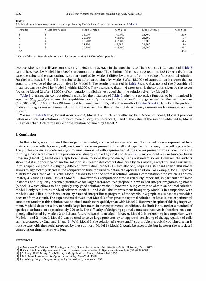
Table 8Solution of the minimal cost reserve selection problem by Models 2 and 3 for artificial instances of Table 5.


1 8 22,000⁄ >15,000 22,700 2292 5 23,600⁄ >15,000 23,400 973 4 19,200⁄ >15,000 19,300 5154 7 21,200 13,983 21,200 185 3 20,500⁄ >15,000 21,000 857Av. 343



average when some cells are compulsory, and 6621 s on average in the opposite case. The instances 1, 3, 4 and 5 of Table 6cannot be solved by Model 2 in 15,000 s of computation time. The solution of the instance 2 requires 12,319 seconds. In thatcase, the value of the near-optimal solution supplied by Model 3 differs by one unit from the value of the optimal solution.For the instances 1, 3, 4 and 5, the value of the solution obtained by Model 2 after 15,000 s of computation is greater than orequal to the value of the solution given by Model 3. The results presented in Table 7 show that none of the 5 consideredinstances can be solved by Model 2 within 15,000 s. They also show that, in 4 cases over 5, the solution given by the solver(by using Model 2) after 15,000 s of computation is slightly less good than the solution given by Model 3.

Table 8 presents the computational results for the instances of Table 6 when the objective function to be minimized isequal to

Pði;jÞ2M�Ndijxij where the acquisition costs dij are randomly and uniformly generated in the set of values

{100,200,300, . . . ,1000}. The CPU time limit has been fixed to 15,000 s. The results of Tables 6 and 8 show that the problemof determining a reserve of minimal cost is rather easier than the problem of determining a reserve with a minimal numberof cells.

We see in Table 8 that, for instances 2 and 4, Model 3 is much more efficient than Model 2. Indeed, Model 3 providesbetter or equivalent solutions and much more quickly. For Instance 1, 3 and 5, the value of the solution obtained by Model3 is at less than 3.2% of the value of the solution obtained by Model 2.

8. Conclusion

In this article, we considered the design of completely connected nature reserves. The studied zone is represented by amatrix of m � n cells. For every cell, we know the species present in the cell and capable of surviving if the cell is protected.The problem consists in determining a minimal number of cells representing all the species present in the studied zone andforming a connected space. This problem was already studied by Önal and Briers [2] who proposed a mixed-integer linearprogram (Model 1), based on a graph formulation, to solve the problem by using a standard solver. However, the authorsshow that it is difficult to obtain the solution in a reasonable computation time by this model, except for small instances.In this paper, we propose a slightly different formulation (Model 2) which also only requires a standard solver. This modelallows to significantly decrease the computation time required to obtain the optimal solution. For example, for 100 speciesdistributed on a zone of 100 cells, Model 2 allows to find the optimal solution within a computation time which is approx-imately 4.5 times as small as with Model 1. However this computation time is relatively important, in particular for someinstances and it quickly becomes prohibitive for larger instances. We propose a new mixed-integer programming model(Model 3) which allows to find quickly very good solutions without, however, being certain to obtain an optimal solution.Model 3 only requires a standard solver as Models 1 and 2 do. The improvement brought by Model 3 in comparison withModels 1 and 2 lies in the formulation, by a mixed-integer linear program, of the search, in a graph, of a subset of arcs whichdoes not form a circuit. The experiments showed that Model 3 often gave the optimal solution (at least in our experimentalconditions) and that this solution was obtained much more quickly than with Model 2. However, in spite of this big improve-ment, Model 3 does not allow to handle large instances. In our experimental conditions, the limit is situated at a hundred ofspecies distributed on approximately 200 cells. The difficulty of designing optimal connected reserves is therefore not com-pletely eliminated by Models 2 and 3 and future research is needed. However, Model 3 is interesting in comparison withModels 1 and 2. Indeed, Model 3 can be used to solve large problems by an approach consisting of the aggregation of cellsas it is proposed by Önal and Briers [2]. With Model 3, the solution of every (small) sub-problem is quickly obtained, what isnot the case with the model proposed by these authors (Model 1). Model 2 would be acceptable, but however the associatedcomputation time is relatively long.

References

[1] A. Moilanen, K.A. Wilson, H.P. Possingham (Eds.), Spatial Conservation Prioritization, Oxford University Press, 2009.[2] H. Önal, R.A. Briers, Optimal selection of a connected reserve network, Operations Research 54 (2006) 379–388.[3] J.A. Bondy, U.S.R. Murty, Graph Theory with Applications, Elsevier Science Ltd, 1976.[4] E.M.L. Beale, Introduction to Optimization, Wiley, New-York, 1988.[5] L.A. Wolsey, Integer Programming, Wiley-Interscience, New York, 1998.


[6] R.S. Garfinkel, Motivation and modeling, in: E.L. Lawler, J.K. Lenstra, A.H.G. Rinnooy Kan, D.B. Shmoys (Eds.), The Traveling Salesman Problem, JohnWiley & Sons, New York, 1985. Ch. 2.

[7] R. Fourer, D.M. Gay, B.W. Kernighan, AMPL, a modeling language for mathematical programming, Boyd & Fraser Publishing Company, Danvers, USA.,1993.

[8] CPLEX, ILOG CPLEX 10.2.0 Reference Manual, ILOG CPLEX Division, Gentilly, France, 2007.[9] MPL Modeling System (4.1), Maximal Software Technology, Arlington, VA 22201, USA.

Documents

Designing an optimal connected nature reserve