Embed Size (px)
Citation preview
3
SAND2004-0522 Unlimited Release Printed June 2004
DESIGN STUDIES FOR TWIST-COUPLED WIND TURBINE BLADES
James Locke and Ulyses Valencia
Wichita State University National Institute for Aviation Research
Wichita, Kansas 67260-0093
Abstract
This study presents results obtained for four hybrid designs of the Northern Power Systems (NPS) 9.2-meter prototype version of the ERS-100 wind turbine rotor blade. The ERS-100 wind turbine rotor blade was designed and developed by TPI composites. The baseline design uses e-glass unidirectional fibers in combination with ±45-degree and random mat layers for the skin and spar cap. This project involves developing structural finite element models of the baseline design and carbon hybrid designs with and without twist-bend coupling. All designs were evaluated for a unit load condition and two extreme wind conditions. The unit load condition was used to evaluate the static deflection, twist and twist-coupling parameter. Maximum deflections and strains were determined for the extreme wind conditions. Linear and nonlinear buckling loads were determined for a tip load condition. The results indicate that carbon fibers can be used to produce twist-coupled designs with comparable deflections, strains and buckling loads to the e-glass baseline.

4
Acknowledgments
This project was supported by Sandia National Laboratories under Contract No. 26964. The authors would like to thank Daniel Laird, Thomas Ashwill and Paul Veers for their guidance and support. The NuMAD training provided by Daniel Laird is very much appreciated.
5
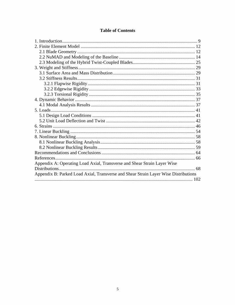
Table of Contents 1. Introduction..................................................................................................................... 9 2. Finite Element Model ................................................................................................... 12
2.1 Blade Geometry ...................................................................................................... 12 2.2 NuMAD and Modeling of the Baseline .................................................................. 14 2.3 Modeling of the Hybrid Twist-Coupled Blades...................................................... 25
3. Weight and Stiffness ..................................................................................................... 29 3.1 Surface Area and Mass Distribution ....................................................................... 29 3.2 Stiffness Results...................................................................................................... 31
3.2.1 Flapwise Rigidity ............................................................................................. 31 3.2.2 Edgewise Rigidity............................................................................................ 33 3.2.3 Torsional Rigidity ............................................................................................ 35
4. Dynamic Behavior ........................................................................................................ 37 4.1 Modal Analysis Results .......................................................................................... 37
5. Loads............................................................................................................................. 41 5.1 Design Load Conditions ......................................................................................... 41 5.2 Unit Load Deflection and Twist ............................................................................. 42
6. Strains ........................................................................................................................... 46 7. Linear Buckling ............................................................................................................ 54 8. Nonlinear Buckling....................................................................................................... 58
8.1 Nonlinear Buckling Analysis.................................................................................. 58 8.2 Nonlinear Buckling Results .................................................................................... 59
Recommendations and Conclusions ................................................................................. 64 References......................................................................................................................... 66 Appendix A: Operating Load Axial, Transverse and Shear Strain Layer Wise Distributions...................................................................................................................... 68 Appendix B: Parked Load Axial, Transverse and Shear Strain Layer Wise Distributions......................................................................................................................................... 102
6
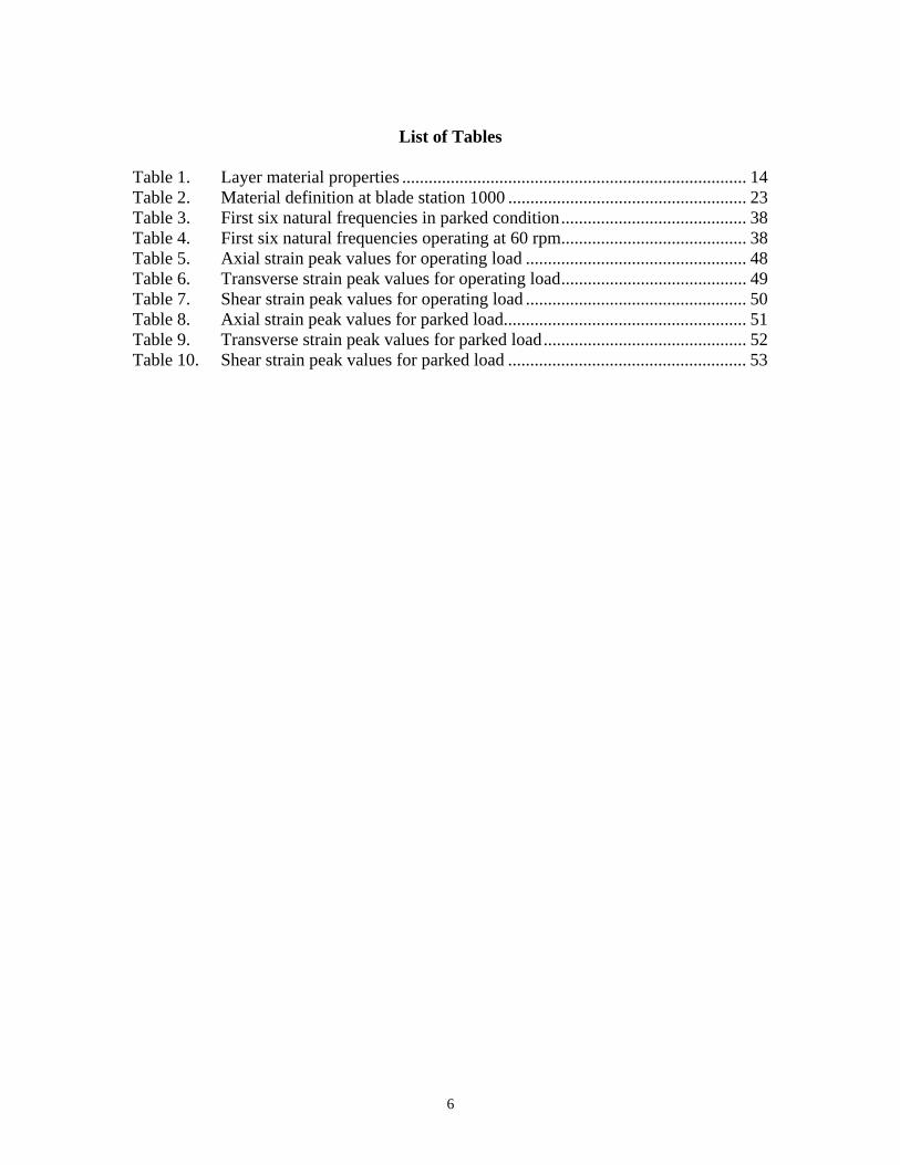
List of Tables
Table 1. Layer material properties .............................................................................. 14 Table 2. Material definition at blade station 1000 ...................................................... 23 Table 3. First six natural frequencies in parked condition.......................................... 38 Table 4. First six natural frequencies operating at 60 rpm.......................................... 38 Table 5. Axial strain peak values for operating load .................................................. 48 Table 6. Transverse strain peak values for operating load.......................................... 49 Table 7. Shear strain peak values for operating load .................................................. 50 Table 8. Axial strain peak values for parked load....................................................... 51 Table 9. Transverse strain peak values for parked load.............................................. 52 Table 10. Shear strain peak values for parked load ...................................................... 53
7
List of Figures
Figure 1. NPS-100 prototype blade planform .......................................................... 12 Figure 2. Chord length distribution .......................................................................... 12 Figure 3. Geometric twist distribution ..................................................................... 13 Figure 4. Typical structural cross section................................................................. 13 Figure 5. Breakdown of material usage in the NPS-100.......................................... 14 Figure 6. Aerodynamic geometry defining station 2200.......................................... 16 Figure 7. Structural geometric defining points at station 2200 ................................ 17 Figure 8. Layer and shear web representation.......................................................... 18 Figure 9. Mesh variations due to numbers of elements and airfoil points. .............. 19 Figure 10. Real constant variations due to airfoil non symmetry vs. symmetry........ 20 Figure 11. NPS-100 stations in mm ........................................................................... 21 Figure 12. NuMAD material definition...................................................................... 22 Figure 13. Blade station 2200 as defined in NuMAD................................................ 23 Figure 14. Blade station 2200 ANSYS model ........................................................... 23 Figure 15. ANSYS finite element model of the NPS-100 ......................................... 24 Figure 16. Coupled lay ups (from Karaolis, Reference 3) ......................................... 25 Figure 17. ANSYS layer stacking sequence for 20 degree carbon substitution......... 26 Figure 18. Spar cap axial stiffness coefficient ........................................................... 27 Figure 19. Spar cap twist-coupling coefficient .......................................................... 27 Figure 20. Required carbon thickness for C520 spar cap layer.................................. 28 Figure 21. Approximate surface area distribution for the NPS-100 prototype blade. 29 Figure 22. Approximate total mass ............................................................................ 30 Figure 23. Approximate mass distribution ................................................................. 30 Figure 24. Application of a 500 lb flapwise tip load.................................................. 31 Figure 25. Flapwise bending angle............................................................................. 32 Figure 26. Flapwise bending stiffness........................................................................ 32 Figure 27. Application of a 500 lb edgewise tip load ................................................ 33 Figure 28. Edgewise bending angle ........................................................................... 34 Figure 29. Edgewise bending stiffness....................................................................... 34 Figure 30. Application of a 1000 N-m torque ............................................................ 35 Figure 31. Torsional twist angle................................................................................. 36 Figure 32. Torsional stiffness..................................................................................... 36 Figure 33. First Mode (flatwise) (top), and Second Mode (edgewise) (bottom) ....... 39 Figure 34. Third Mode (Top)(mixed), and Fourth Mode (bottom) (mixed) .............. 40 Figure 35. Flapwise Bending Moment ....................................................................... 41 Figure 36. Blade bending deflection .......................................................................... 42 Figure 37. Twist Angle Comparison for the NPS-100 with 1000lb (4-250 lb load)
distributed load applied at 3, 4.5, 6.5 and 8m. .......................................................... 43 Figure 38. Twist-coupling parameter β ...................................................................... 45 Figure 39. High strain areas shown by arrows ........................................................... 46 Figure 40. NPS-100 baseline linear buckling............................................................. 54 Figure 41. NPS-100 0-degree carbon linear buckling................................................ 55 Figure 42. NPS-100 15-degree carbon linear buckling.............................................. 55
8
Figure 43. NPS-100 20-degree carbon linear buckling.............................................. 56 Figure 44. Linear buckling root bending moment...................................................... 57 Figure 45. Loading scheme for the nonlinear analysis............................................... 59 Figure 46. NPS-100 0-degree carbon nonlinear buckling load factor versus
cumulative iterations................................................................................................. 60 Figure 47. NPS-100 0-degree carbon nonlinear buckling load factor versus tip
deflection……………………………………………………………………………60 Figure 48. NPS-100 15-degree carbon nonlinear buckling load factor versus
cumulative iterations................................................................................................. 61 Figure 49. NPS-100 15-degree carbon nonlinear buckling load factor versus tip
deflection……………………………………………………………………………61 Figure 50. NPS-100 20-degree carbon nonlinear buckling load factor versus
cumulative iterations................................................................................................. 62 Figure 51. NPS-100 20-degree carbon nonlinear buckling load factor versus tip
deflection……………………………………………………………………………62 Figure 52. Nonlinear buckling root bending moment ................................................ 63
9
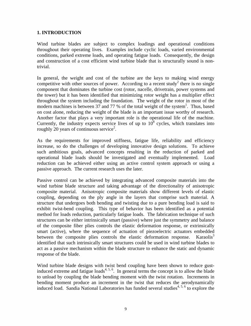
1. INTRODUCTION Wind turbine blades are subject to complex loadings and operational conditions throughout their operating lives. Examples include cyclic loads, varied environmental conditions, parked extreme loads, and operating fatigue loads. Consequently, the design and construction of a cost efficient wind turbine blade that is structurally sound is non-trivial. In general, the weight and cost of the turbine are the keys to making wind energy competitive with other sources of power. According to a recent study2 there is no single component that dominates the turbine cost (rotor, nacelle, drivetrain, power systems and the tower) but it has been identified that minimizing rotor weight has a multiplier effect throughout the system including the foundation. The weight of the rotor in most of the modern machines is between 37 and 77 % of the total weight of the system1. Thus, based on cost alone, reducing the weight of the blade is an important issue worthy of research. Another factor that plays a very important role is the operational life of the machine. Currently, the industry expects service lives of up to 108 cycles, which translates into roughly 20 years of continuous service2. As the requirements for improved stiffness, fatigue life, reliability and efficiency increase, so do the challenges of developing innovative design solutions. To achieve such ambitious goals, advanced concepts resulting in the reduction of parked and operational blade loads should be investigated and eventually implemented. Load reduction can be achieved either using an active control system approach or using a passive approach. The current research uses the later. Passive control can be achieved by integrating advanced composite materials into the wind turbine blade structure and taking advantage of the directionality of anisotropic composite material. Anisotropic composite materials show different levels of elastic coupling, depending on the ply angle in the layers that comprise such material. A structure that undergoes both bending and twisting due to a pure bending load is said to exhibit twist-bend coupling. This type of behavior has been identified as a potential method for loads reduction, particularly fatigue loads. The fabrication technique of such structures can be either intrinsically smart (passive) where just the symmetry and balance of the composite fiber plies controls the elastic deformation response, or extrinsically smart (active), where the sequence of actuation of piezoelectric actuators embedded between the composite plies controls the elastic deformation response. Karaolis3 identified that such intrinsically smart structures could be used in wind turbine blades to act as a passive mechanism within the blade structure to enhance the static and dynamic response of the blade. Wind turbine blade designs with twist bend coupling have been shown to reduce gust-induced extreme and fatigue loads4, 5, 6. In general terms the concept is to allow the blade to unload by coupling the blade bending moment with the twist rotation. Increments in bending moment produce an increment in the twist that reduces the aerodynamically induced load. Sandia National Laboratories has funded several studies4, 5, 6 to explore the
10
overall benefits of the twist-coupled blades. The results of these studies indicate that a 10% decrease in fatigue loads throughout the system can be achieved with high levels of coupling, but with relatively low levels of twist. The overall level of load reduction depends on the loading environment and the amount of coupling in the structural material. Ong and Tsai7, 8, 9 at Stanford University have conducted initial studies in material usage, design and manufacturing. These studies suggest that there is a need for higher stiffness fibers to produce significant coupling. The requirement for higher blade stiffness means that conventional glass fiber materials must be fully or partially replaced with carbon fibers. Carbon fibers are not currently used on most commercial wind turbine blades because carbon is more costly than glass, and blades with a combination of glass and carbon could have areas with significant strain concentrations and potential fatigue problems. These detailed design issues must be further studied before twist coupling is implemented by the wind industry. The challenge is to manufacture a cost effective and durable blade that meets or exceeds all certification requirements. Studies performed by Mike Zuteck Consulting, Wichita State University, and Global Energy Concepts10, have addressed major issues related to the implementation of bend-twist coupling. The results suggest that there is a good possibility that twist coupled blades can be successfully manufactured, but the detailed design issues still need to be resolved. Potential blade designs (including material choice, fiber placement, and internal structure) need to be evaluated in order to define a cost effective and durable twist-coupled blade. As part of these combined efforts to further investigate the feasibility of bend-twist coupled blades, Wichita State University has been contracted by Sandia National Laboratories to evaluate the performance of a conventional glass blade design compared with bend-twist coupled designs. For this study a finite element model of an existing prototype blade, the NPS-100 manufactured for Northern Power Systems by TPI Composites of Warren, RI, has been created and used as a baseline for all calculations and comparisons. The main objectives of this work are to:
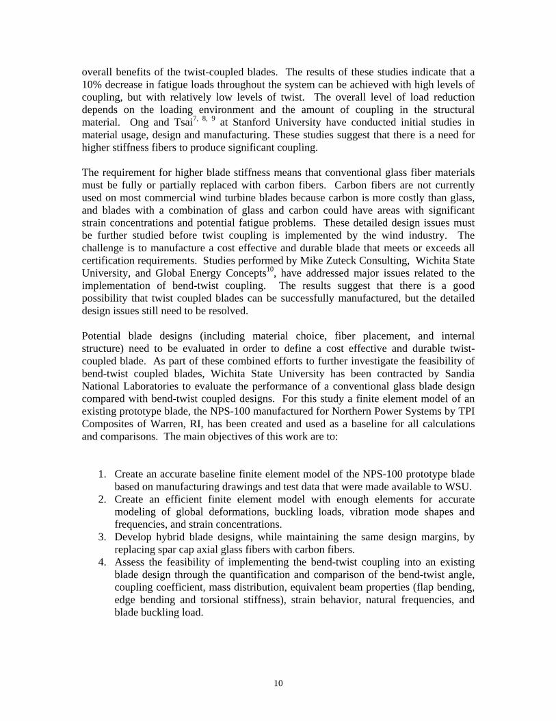
1. Create an accurate baseline finite element model of the NPS-100 prototype blade based on manufacturing drawings and test data that were made available to WSU.
2. Create an efficient finite element model with enough elements for accurate modeling of global deformations, buckling loads, vibration mode shapes and frequencies, and strain concentrations.
3. Develop hybrid blade designs, while maintaining the same design margins, by replacing spar cap axial glass fibers with carbon fibers.
4. Assess the feasibility of implementing the bend-twist coupling into an existing blade design through the quantification and comparison of the bend-twist angle, coupling coefficient, mass distribution, equivalent beam properties (flap bending, edge bending and torsional stiffness), strain behavior, natural frequencies, and blade buckling load.

11
This report summarizes the finite element modeling and corresponding results for the baseline and hybrid NPS-100 blade finite element models. Different degrees of bend-twist coupling have been implemented through the replacement of spar cap axial glass fibers with carbon fibers at different orientations. Although this is not an optimum design, it is a good starting point for examining the detailed issues of a carbon hybrid, twist coupled derivative of the NPS-100 blade. All results are based on ANSYS shell finite elements models that were developed using the Numerical Manufacturing and Design tool (NuMAD)11.
12
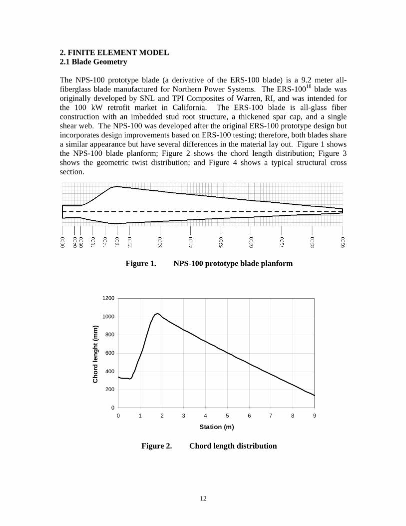
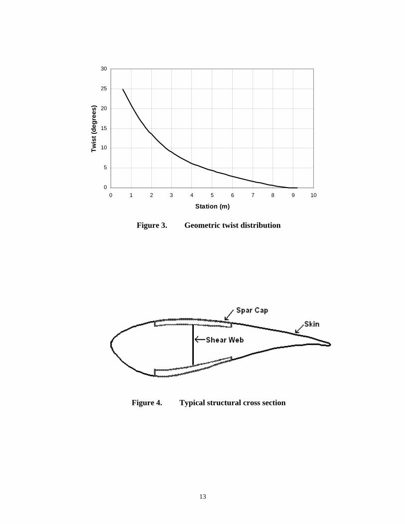
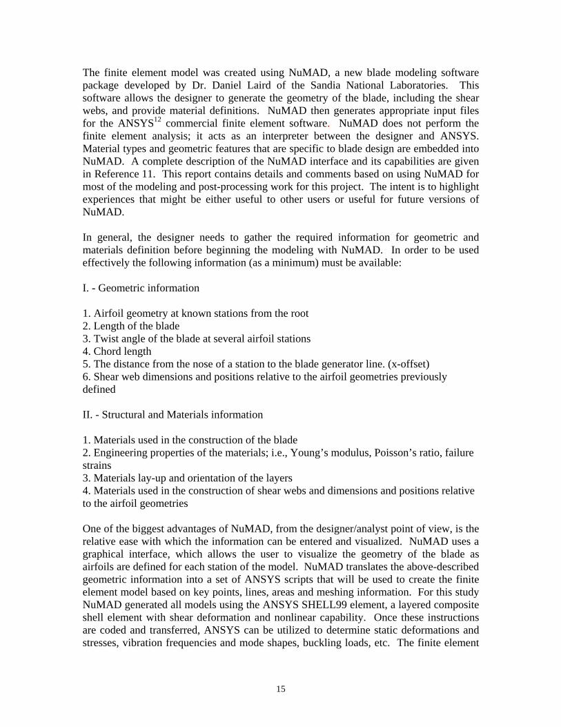
2. FINITE ELEMENT MODEL 2.1 Blade Geometry The NPS-100 prototype blade (a derivative of the ERS-100 blade) is a 9.2 meter all-fiberglass blade manufactured for Northern Power Systems. The ERS-10018 blade was originally developed by SNL and TPI Composites of Warren, RI, and was intended for the 100 kW retrofit market in California. The ERS-100 blade is all-glass fiber construction with an imbedded stud root structure, a thickened spar cap, and a single shear web. The NPS-100 was developed after the original ERS-100 prototype design but incorporates design improvements based on ERS-100 testing; therefore, both blades share a similar appearance but have several differences in the material lay out. Figure 1 shows the NPS-100 blade planform; Figure 2 shows the chord length distribution; Figure 3 shows the geometric twist distribution; and Figure 4 shows a typical structural cross section.
Figure 1. NPS-100 prototype blade planform
0
200
400
600
800
1000
1200
0 1 2 3 4 5 6 7 8 9
Station (m)
Cho
rd le
nght
(mm
)
Figure 2. Chord length distribution
13
0
5
10
15
20
25
30
0 1 2 3 4 5 6 7 8 9 10
Station (m)
Twis
t (de
gree
s)
Figure 3. Geometric twist distribution
Figure 4. Typical structural cross section

14
2.2 NuMAD and Modeling of the Baseline The NPS-100 prototype design consists of a surface gel coat, e-glass unidirectional fibers, ±45-degree and random mat layers for the skin and spar cap. Balsa core material is also used in the trailing edge and the spar shear web. Figure 5 and Table 1 describe the breakdown of material usage in the spar caps as a function of blade section. The terminology used in Table 1 and Figure 5 is defined as follows: C520 for e-glass unidirectional fibers, C260 for the lower stiffness glass fibers used in the ±45º layers, ¾ Mat for random mat glass fibers, Gel Coat for the thin layer of surface coating material, DBM1208 for 3 layers of material as described in Table 1, and DBM1708 for 3 layers of material as described in Table 1.
0
1
2
3
4
5
6
7
8
9
10
1.0 1.4 3.2 7.2 8.2
Blade Radial STA, m
Thic
knes
s, m
m
C520
DBM1208
DBM1708
3/4 Mat
Gel Coat
Figure 5. Breakdown of material usage in the NPS-100
Material E1,
GPa E2, GPa
G12, GPa
ν12
C520 48.2 11.7 6.48 0.30 C260 43.0 8.90 4.50 0.27 ¾ Mat 7.58 7.58 6.48 0.30 Gel Coat 3.44 3.44 1.32 0.30 Carbon 130 10.3 7.17 0.28 DBM1208 3 layers
+45º Fiberglass (0.186 mm)/ ¾ Mat (0.186 mm)/ -45º Fiberglass (0.186 mm)
DBM1708 3 layers
+45º Fiberglass (0.296 mm)/ ¾ Mat (0.296 mm)/ -45º Fiberglass (0.296 mm)
Table 1. Layer material properties
15
The finite element model was created using NuMAD, a new blade modeling software package developed by Dr. Daniel Laird of the Sandia National Laboratories. This software allows the designer to generate the geometry of the blade, including the shear webs, and provide material definitions. NuMAD then generates appropriate input files for the ANSYS12 commercial finite element software. NuMAD does not perform the finite element analysis; it acts as an interpreter between the designer and ANSYS. Material types and geometric features that are specific to blade design are embedded into NuMAD. A complete description of the NuMAD interface and its capabilities are given in Reference 11. This report contains details and comments based on using NuMAD for most of the modeling and post-processing work for this project. The intent is to highlight experiences that might be either useful to other users or useful for future versions of NuMAD. In general, the designer needs to gather the required information for geometric and materials definition before beginning the modeling with NuMAD. In order to be used effectively the following information (as a minimum) must be available: I. - Geometric information 1. Airfoil geometry at known stations from the root 2. Length of the blade 3. Twist angle of the blade at several airfoil stations 4. Chord length 5. The distance from the nose of a station to the blade generator line. (x-offset) 6. Shear web dimensions and positions relative to the airfoil geometries previously defined II. - Structural and Materials information 1. Materials used in the construction of the blade 2. Engineering properties of the materials; i.e., Young’s modulus, Poisson’s ratio, failure strains 3. Materials lay-up and orientation of the layers 4. Materials used in the construction of shear webs and dimensions and positions relative to the airfoil geometries One of the biggest advantages of NuMAD, from the designer/analyst point of view, is the relative ease with which the information can be entered and visualized. NuMAD uses a graphical interface, which allows the user to visualize the geometry of the blade as airfoils are defined for each station of the model. NuMAD translates the above-described geometric information into a set of ANSYS scripts that will be used to create the finite element model based on key points, lines, areas and meshing information. For this study NuMAD generated all models using the ANSYS SHELL99 element, a layered composite shell element with shear deformation and nonlinear capability. Once these instructions are coded and transferred, ANSYS can be utilized to determine static deformations and stresses, vibration frequencies and mode shapes, buckling loads, etc. The finite element
16
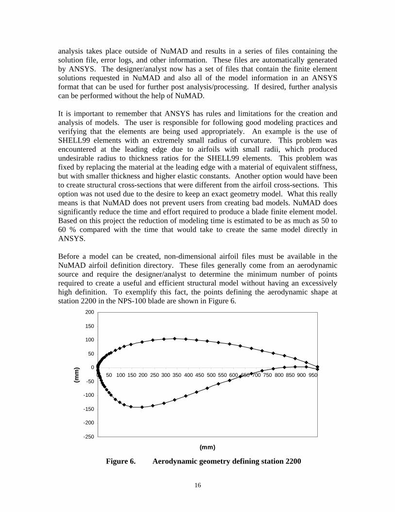
analysis takes place outside of NuMAD and results in a series of files containing the solution file, error logs, and other information. These files are automatically generated by ANSYS. The designer/analyst now has a set of files that contain the finite element solutions requested in NuMAD and also all of the model information in an ANSYS format that can be used for further post analysis/processing. If desired, further analysis can be performed without the help of NuMAD. It is important to remember that ANSYS has rules and limitations for the creation and analysis of models. The user is responsible for following good modeling practices and verifying that the elements are being used appropriately. An example is the use of SHELL99 elements with an extremely small radius of curvature. This problem was encountered at the leading edge due to airfoils with small radii, which produced undesirable radius to thickness ratios for the SHELL99 elements. This problem was fixed by replacing the material at the leading edge with a material of equivalent stiffness, but with smaller thickness and higher elastic constants. Another option would have been to create structural cross-sections that were different from the airfoil cross-sections. This option was not used due to the desire to keep an exact geometry model. What this really means is that NuMAD does not prevent users from creating bad models. NuMAD does significantly reduce the time and effort required to produce a blade finite element model. Based on this project the reduction of modeling time is estimated to be as much as 50 to 60 % compared with the time that would take to create the same model directly in ANSYS. Before a model can be created, non-dimensional airfoil files must be available in the NuMAD airfoil definition directory. These files generally come from an aerodynamic source and require the designer/analyst to determine the minimum number of points required to create a useful and efficient structural model without having an excessively high definition. To exemplify this fact, the points defining the aerodynamic shape at station 2200 in the NPS-100 blade are shown in Figure 6.
-250
-200
-150
-100
-50
0
50
100
150
200
0 50 100 150 200 250 300 350 400 450 500 550 600 650 700 750 800 850 900 950
(mm)
(mm
)
Figure 6. Aerodynamic geometry defining station 2200
17
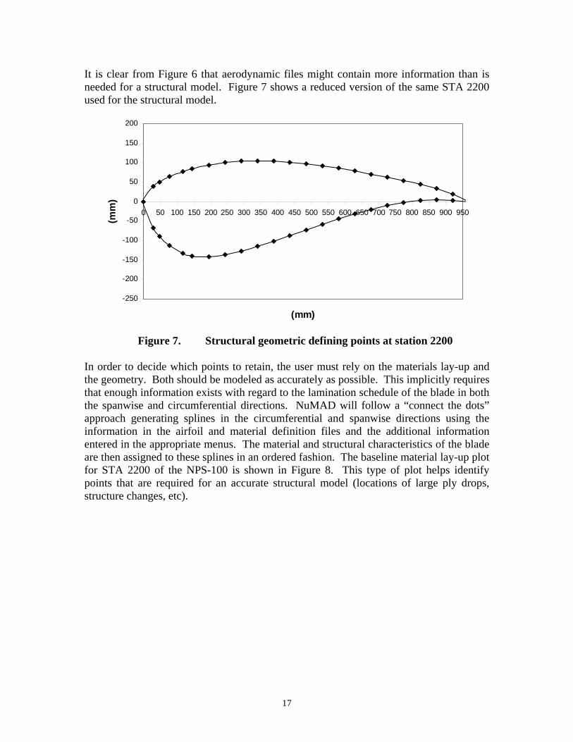
It is clear from Figure 6 that aerodynamic files might contain more information than is needed for a structural model. Figure 7 shows a reduced version of the same STA 2200 used for the structural model.
-250
-200
-150
-100
-50
0
50
100
150
200
0 50 100 150 200 250 300 350 400 450 500 550 600 650 700 750 800 850 900 950
(mm)
(mm
)
Figure 7. Structural geometric defining points at station 2200
In order to decide which points to retain, the user must rely on the materials lay-up and the geometry. Both should be modeled as accurately as possible. This implicitly requires that enough information exists with regard to the lamination schedule of the blade in both the spanwise and circumferential directions. NuMAD will follow a “connect the dots” approach generating splines in the circumferential and spanwise directions using the information in the airfoil and material definition files and the additional information entered in the appropriate menus. The material and structural characteristics of the blade are then assigned to these splines in an ordered fashion. The baseline material lay-up plot for STA 2200 of the NPS-100 is shown in Figure 8. This type of plot helps identify points that are required for an accurate structural model (locations of large ply drops, structure changes, etc).
18
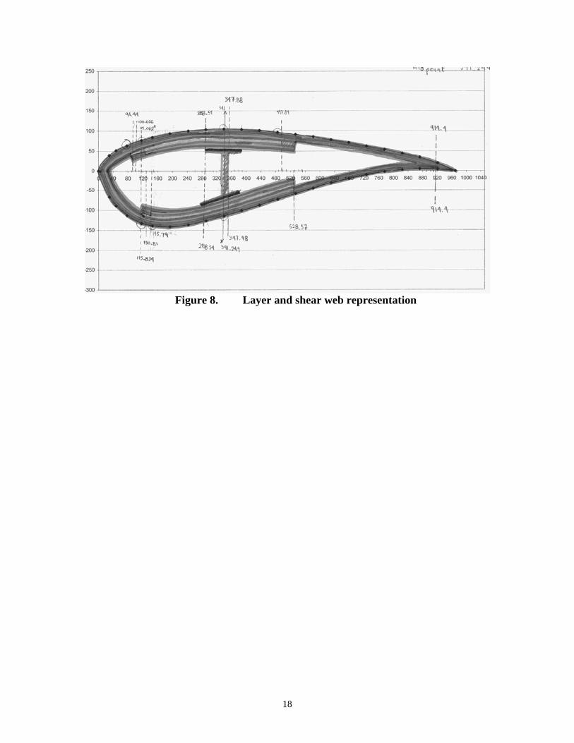
Figure 8. Layer and shear web representation
19
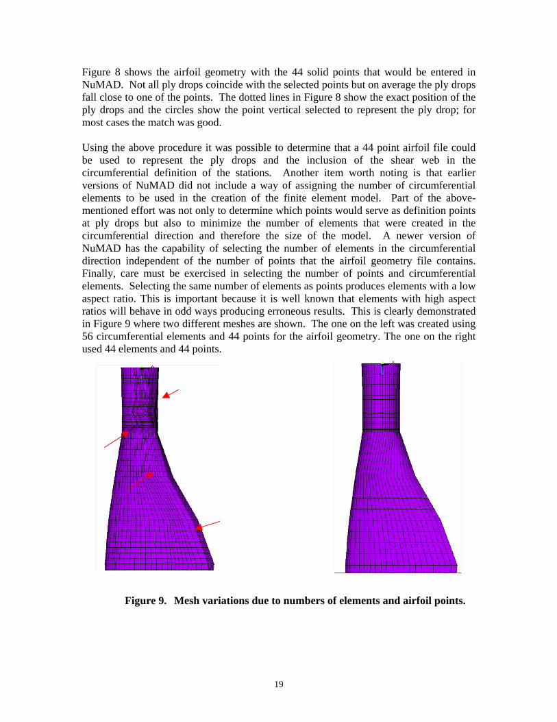
Figure 8 shows the airfoil geometry with the 44 solid points that would be entered in NuMAD. Not all ply drops coincide with the selected points but on average the ply drops fall close to one of the points. The dotted lines in Figure 8 show the exact position of the ply drops and the circles show the point vertical selected to represent the ply drop; for most cases the match was good. Using the above procedure it was possible to determine that a 44 point airfoil file could be used to represent the ply drops and the inclusion of the shear web in the circumferential definition of the stations. Another item worth noting is that earlier versions of NuMAD did not include a way of assigning the number of circumferential elements to be used in the creation of the finite element model. Part of the above-mentioned effort was not only to determine which points would serve as definition points at ply drops but also to minimize the number of elements that were created in the circumferential direction and therefore the size of the model. A newer version of NuMAD has the capability of selecting the number of elements in the circumferential direction independent of the number of points that the airfoil geometry file contains. Finally, care must be exercised in selecting the number of points and circumferential elements. Selecting the same number of elements as points produces elements with a low aspect ratio. This is important because it is well known that elements with high aspect ratios will behave in odd ways producing erroneous results. This is clearly demonstrated in Figure 9 where two different meshes are shown. The one on the left was created using 56 circumferential elements and 44 points for the airfoil geometry. The one on the right used 44 elements and 44 points.
Figure 9. Mesh variations due to numbers of elements and airfoil points.
20
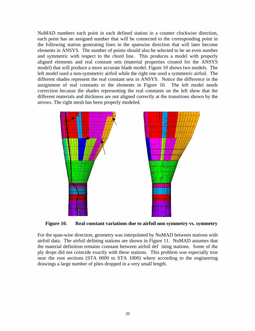
NuMAD numbers each point in each defined station in a counter clockwise direction, each point has an assigned number that will be connected to the corresponding point in the following station generating lines in the spanwise direction that will later become elements in ANSYS. The number of points should also be selected to be an even number and symmetric with respect to the chord line. This produces a model with properly aligned elements and real constant sets (material properties created for the ANSYS model) that will produce a more accurate blade model. Figure 10 shows two models. The left model used a non-symmetric airfoil while the right one used a symmetric airfoil. The different shades represent the real constant sets in ANSYS. Notice the difference in the assignment of real constants to the elements in Figure 10. The left model needs correction because the shades representing the real constants on the left show that the different materials and thickness are not aligned correctly at the transitions shown by the arrows. The right mesh has been properly modeled.
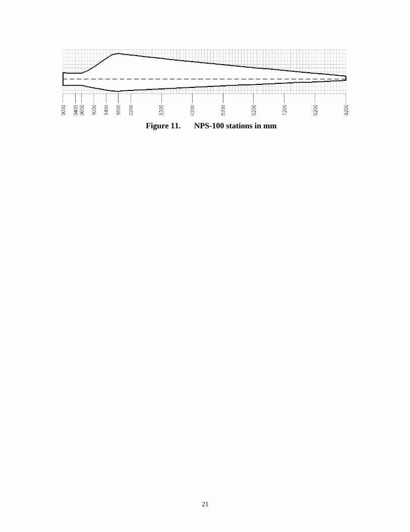
Figure 10. Real constant variations due to airfoil non symmetry vs. symmetry For the span-wise direction, geometry was interpolated by NuMAD between stations with airfoil data. The airfoil defining stations are shown in Figure 11. NuMAD assumes that the material definition remains constant between airfoil def ining stations. Some of the ply drops did not coincide exactly with these stations. This problem was especially true near the root sections (STA 0000 to STA 1000) where according to the engineering drawings a large number of plies dropped in a very small length.
21
Figure 11. NPS-100 stations in mm
22
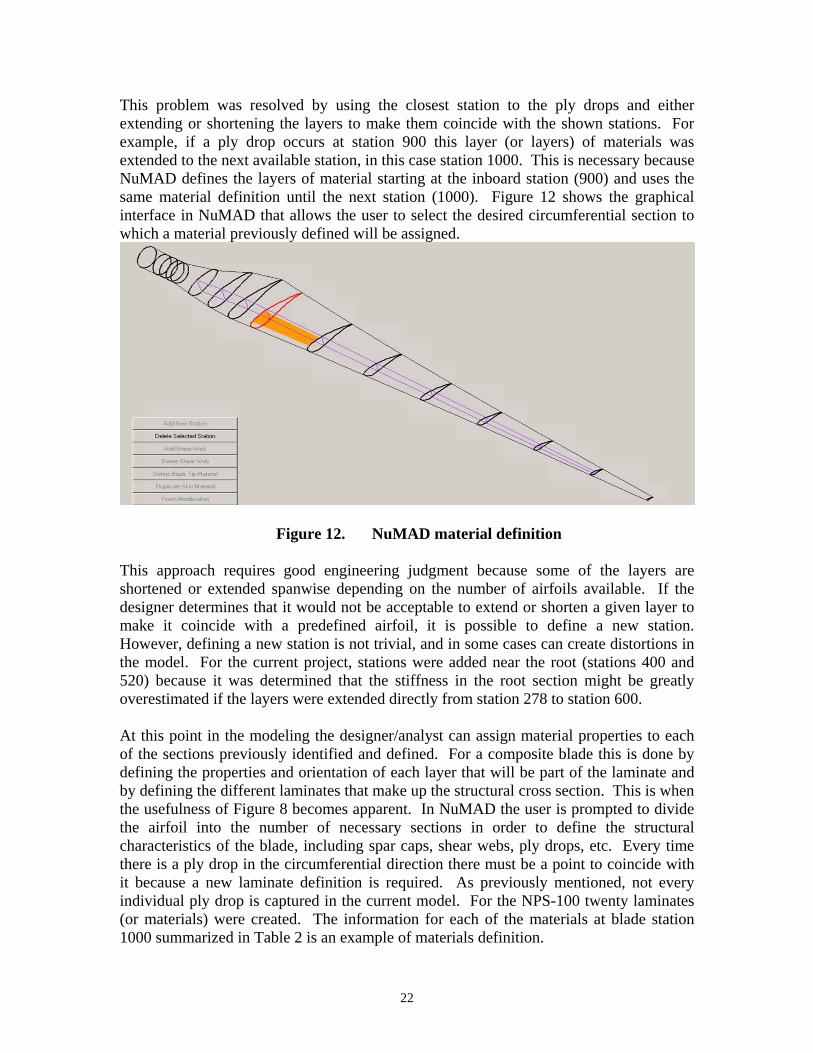
This problem was resolved by using the closest station to the ply drops and either extending or shortening the layers to make them coincide with the shown stations. For example, if a ply drop occurs at station 900 this layer (or layers) of materials was extended to the next available station, in this case station 1000. This is necessary because NuMAD defines the layers of material starting at the inboard station (900) and uses the same material definition until the next station (1000). Figure 12 shows the graphical interface in NuMAD that allows the user to select the desired circumferential section to which a material previously defined will be assigned.
Figure 12. NuMAD material definition This approach requires good engineering judgment because some of the layers are shortened or extended spanwise depending on the number of airfoils available. If the designer determines that it would not be acceptable to extend or shorten a given layer to make it coincide with a predefined airfoil, it is possible to define a new station. However, defining a new station is not trivial, and in some cases can create distortions in the model. For the current project, stations were added near the root (stations 400 and 520) because it was determined that the stiffness in the root section might be greatly overestimated if the layers were extended directly from station 278 to station 600. At this point in the modeling the designer/analyst can assign material properties to each of the sections previously identified and defined. For a composite blade this is done by defining the properties and orientation of each layer that will be part of the laminate and by defining the different laminates that make up the structural cross section. This is when the usefulness of Figure 8 becomes apparent. In NuMAD the user is prompted to divide the airfoil into the number of necessary sections in order to define the structural characteristics of the blade, including spar caps, shear webs, ply drops, etc. Every time there is a ply drop in the circumferential direction there must be a point to coincide with it because a new laminate definition is required. As previously mentioned, not every individual ply drop is captured in the current model. For the NPS-100 twenty laminates (or materials) were created. The information for each of the materials at blade station 1000 summarized in Table 2 is an example of materials definition.
23
Material Number Layer I II III IV V
1 Gelcoat Gelcoat Gelcoat Gelcoat Gelcoat 2 3/4 Mat 3/4 Mat 3/4 Mat 3/4 Mat 3/4 Mat 3 DBM1708 DBM1708 DBM1708 DBM1708 DBM1708 4 DBM1208 DBM1208 DBM1208 DBM1208 Balsa (Aft Panel Balsa)5 Balsa (Nose Balsa) C520 C520 C520 DBM1208 6 DBM1208 C520 C520 C520 7 DBM1708 C520 C520 C520 8 C520 C520 C520 9 C520 C520 C520
10 C520 C520 C520 11 DBM1208 DBM1208 DBM1208 12 DBM1708 DBM1708 DBM1708 13 DBM1708 14 DBM1708 15 DBM1708 16 DBM1708
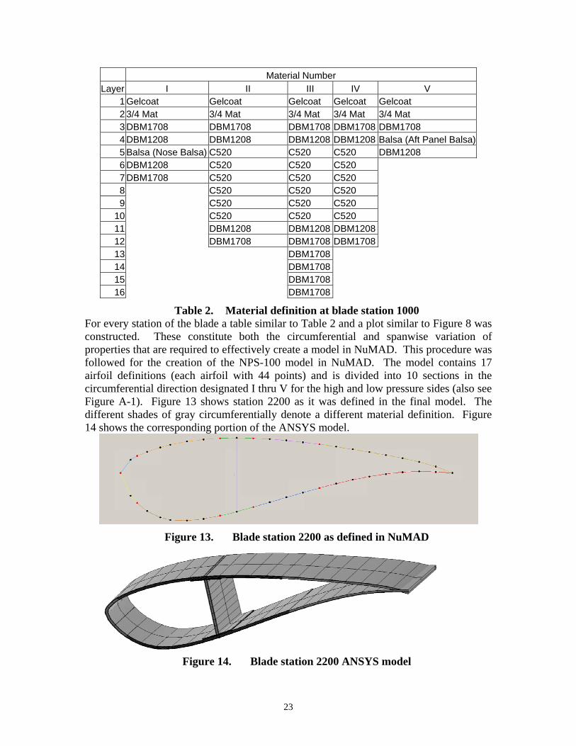
Table 2. Material definition at blade station 1000 For every station of the blade a table similar to Table 2 and a plot similar to Figure 8 was constructed. These constitute both the circumferential and spanwise variation of properties that are required to effectively create a model in NuMAD. This procedure was followed for the creation of the NPS-100 model in NuMAD. The model contains 17 airfoil definitions (each airfoil with 44 points) and is divided into 10 sections in the circumferential direction designated I thru V for the high and low pressure sides (also see Figure A-1). Figure 13 shows station 2200 as it was defined in the final model. The different shades of gray circumferentially denote a different material definition. Figure 14 shows the corresponding portion of the ANSYS model.
Figure 13. Blade station 2200 as defined in NuMAD
Figure 14. Blade station 2200 ANSYS model
24
Using this same modeling approach, three more models were created using NuMAD.
• 0 degrees carbon substitution • 15 degrees carbon substitution • 20 degrees carbon substitution
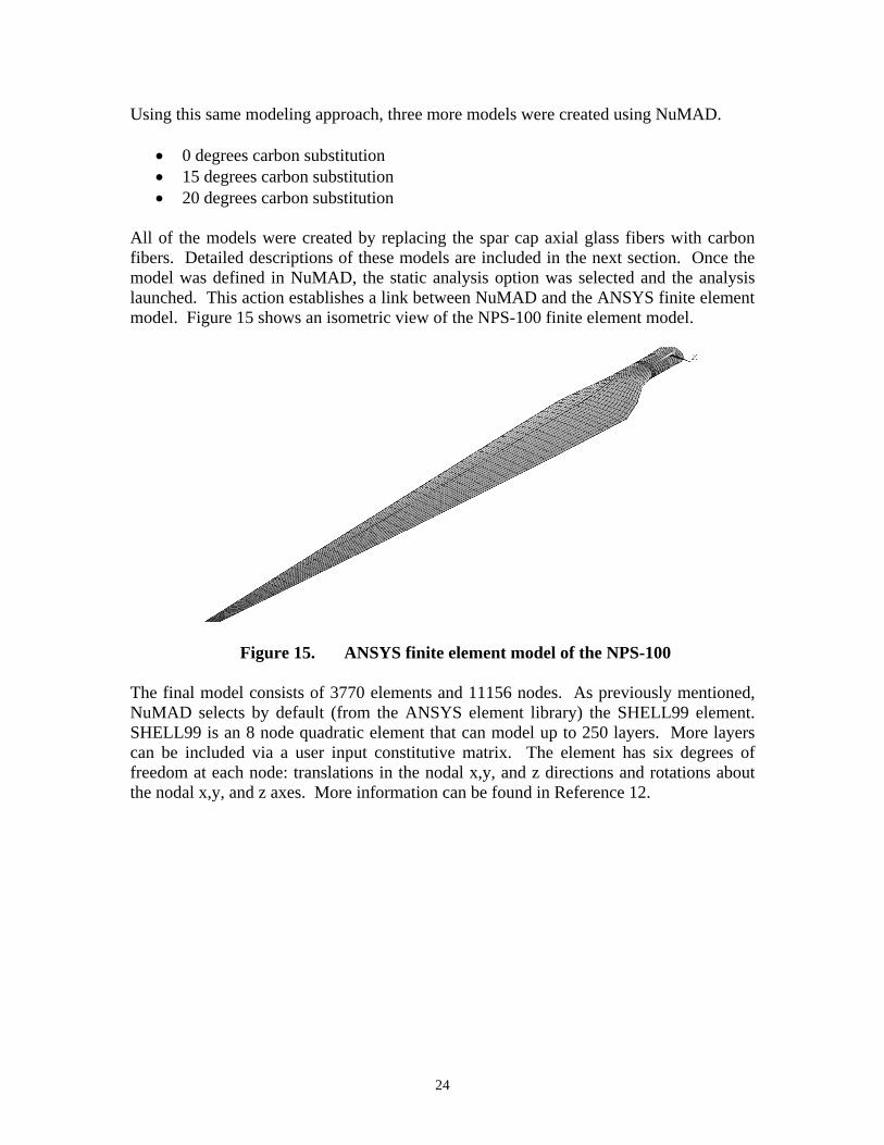
All of the models were created by replacing the spar cap axial glass fibers with carbon fibers. Detailed descriptions of these models are included in the next section. Once the model was defined in NuMAD, the static analysis option was selected and the analysis launched. This action establishes a link between NuMAD and the ANSYS finite element model. Figure 15 shows an isometric view of the NPS-100 finite element model.
Figure 15. ANSYS finite element model of the NPS-100 The final model consists of 3770 elements and 11156 nodes. As previously mentioned, NuMAD selects by default (from the ANSYS element library) the SHELL99 element. SHELL99 is an 8 node quadratic element that can model up to 250 layers. More layers can be included via a user input constitutive matrix. The element has six degrees of freedom at each node: translations in the nodal x,y, and z directions and rotations about the nodal x,y, and z axes. More information can be found in Reference 12.

25
2.3 Modeling of the Hybrid Twist-Coupled Blades The main objective of this project is to evaluate the feasibility of implementing the twist-coupled designs into an existing blade. The all-glass NPS-100 prototype blade is the baseline for all comparisons. Twist-coupling can be introduced either geometrically (using blade sweep) or by using unbalanced off axis fibers oriented at an angle θ with respect to the primary loading direction. The off axis fibers result in extensional-shear coupling at the layer level with either twist bend or twist extensional coupling at the blade level. These two types of coupling are depicted in Figure 16. The mirror symmetric lay-up, shown in Figure 16a, produces twist bend coupling.
Figure 16. Coupled lay ups (from Karaolis, Reference 3) For the present study the mirror lay up, Figure 16a, is implemented by changing the C520 unidirectional fibers in the spar caps to off-axis carbon fibers. GEC10 used a similar approach to implement twist-bend coupling for a conventional design. Their results demonstrate that spar cap off-axis carbon fibers are very effective for small amounts of twist. Two key advantages in using this approach are: 1) the same basic manufacturing technology can be employed to produce the blades, and 2) a carbon-hybrid design uses a limited amount of the more expensive carbon material. NuMAD’s capability to assign different orientations to each of the originally defined layers of material was used to define the mirror lay up. The procedure followed was to use the original baseline model and replace the layers of C520 in the spar caps with carbon and then modify the orientation θ of the selected layers. Figure 17 shows one of the element layer stacking sequences generated in ANSYS for the 20-degree carbon substitution on the low-pressure side of the blade.

26
Figure 17. ANSYS layer stacking sequence for 20 degree carbon substitution A beam theory model13 was used to evaluate the effect of replacing the spar cap unidirectional C520 material with carbon fibers oriented at an angle θ . The beam theory model relates N , the axial force per unit width in the spar caps, to the axial strain, ε , and the shear flow, q :
qN 21 βεβ += (1) where the constants 1β and 2β , in terms of the classical lamination theory ][A matrix14, are given as
1
22
226
664
422
2612162
4
22
22
212
111 ,
−
⎟⎟⎠
⎞⎜⎜⎝
⎛−=
⎟⎟⎠
⎞⎜⎜⎝
⎛−=−−=
AA
A
AAA
AAAA
β
ββββ
β
(2)
and the coefficients of the ][A matrix for an N-layer laminate are defined as:
( )∑=
=N
kkkijij tQA
1 (3)
where ( )
kijQ = transformed reduced stiffness, kt = layer thickness (4)
27
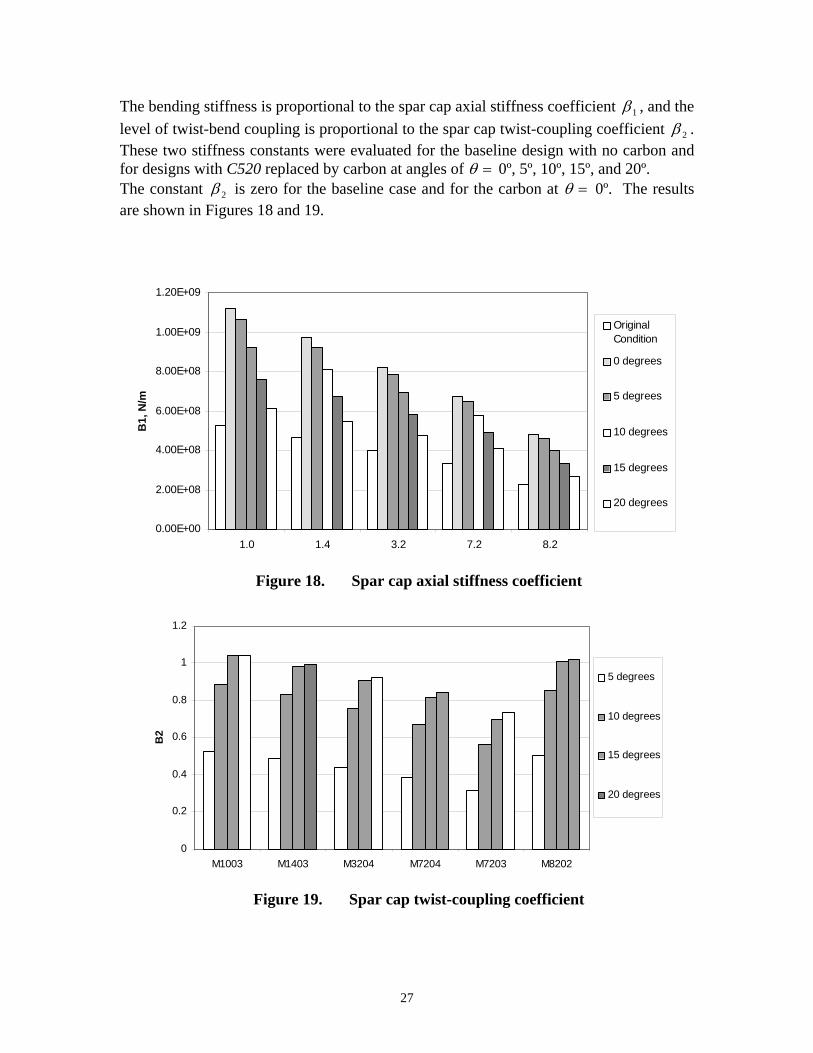
The bending stiffness is proportional to the spar cap axial stiffness coefficient 1β , and the level of twist-bend coupling is proportional to the spar cap twist-coupling coefficient 2β . These two stiffness constants were evaluated for the baseline design with no carbon and for designs with C520 replaced by carbon at angles of =θ 0º, 5º, 10º, 15º, and 20º. The constant 2β is zero for the baseline case and for the carbon at =θ 0º. The results are shown in Figures 18 and 19.
0.00E+00
2.00E+08
4.00E+08
6.00E+08
8.00E+08
1.00E+09
1.20E+09
1.0 1.4 3.2 7.2 8.2
B1,
N/m
OriginalCondition
0 degrees
5 degrees
10 degrees
15 degrees
20 degrees
Figure 18. Spar cap axial stiffness coefficient
0
0.2
0.4
0.6
0.8
1
1.2
M1003 M1403 M3204 M7204 M7203 M8202
B2
5 degrees
10 degrees
15 degrees
20 degrees
Figure 19. Spar cap twist-coupling coefficient
28
As shown in Figure 18, the maximum spar cap axial stiffness coefficient is for the carbon at =θ 0º; whereas, the maximum spar cap twist-coupling coefficient is for the carbon at
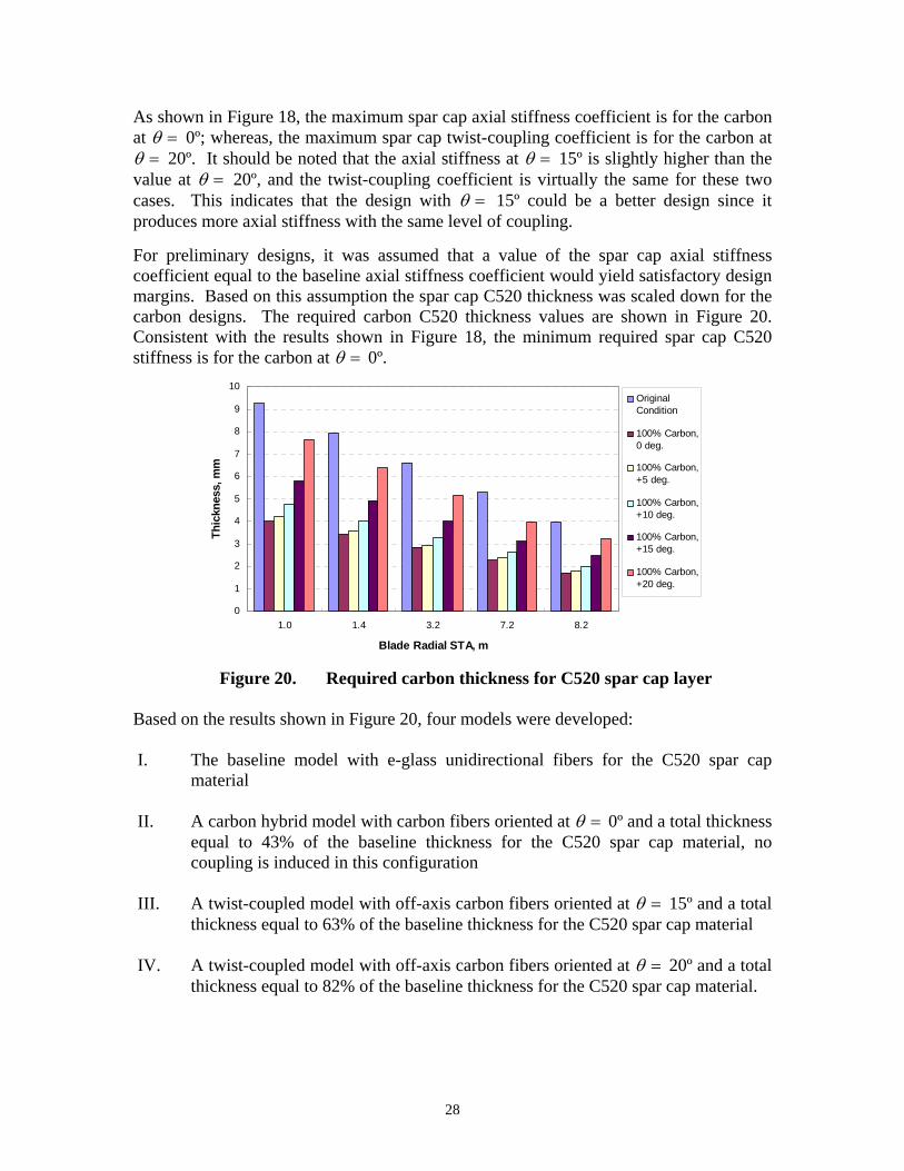
=θ 20º. It should be noted that the axial stiffness at =θ 15º is slightly higher than the value at =θ 20º, and the twist-coupling coefficient is virtually the same for these two cases. This indicates that the design with =θ 15º could be a better design since it produces more axial stiffness with the same level of coupling. For preliminary designs, it was assumed that a value of the spar cap axial stiffness coefficient equal to the baseline axial stiffness coefficient would yield satisfactory design margins. Based on this assumption the spar cap C520 thickness was scaled down for the carbon designs. The required carbon C520 thickness values are shown in Figure 20. Consistent with the results shown in Figure 18, the minimum required spar cap C520 stiffness is for the carbon at =θ 0º.
0
1
2
3
4
5
6
7
8
9
10
1.0 1.4 3.2 7.2 8.2
Blade Radial STA, m
Thic
knes
s, m
m
OriginalCondition
100% Carbon,0 deg.
100% Carbon,+5 deg.
100% Carbon,+10 deg.
100% Carbon,+15 deg.
100% Carbon,+20 deg.
Figure 20. Required carbon thickness for C520 spar cap layer
Based on the results shown in Figure 20, four models were developed: I. The baseline model with e-glass unidirectional fibers for the C520 spar cap
material II. A carbon hybrid model with carbon fibers oriented at =θ 0º and a total thickness
equal to 43% of the baseline thickness for the C520 spar cap material, no coupling is induced in this configuration
III. A twist-coupled model with off-axis carbon fibers oriented at =θ 15º and a total
thickness equal to 63% of the baseline thickness for the C520 spar cap material IV. A twist-coupled model with off-axis carbon fibers oriented at =θ 20º and a total
thickness equal to 82% of the baseline thickness for the C520 spar cap material.
29
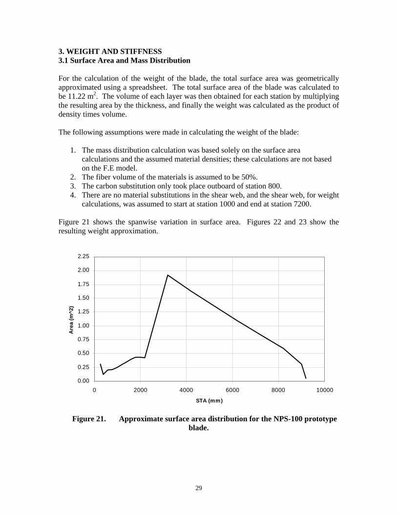
3. WEIGHT AND STIFFNESS 3.1 Surface Area and Mass Distribution For the calculation of the weight of the blade, the total surface area was geometrically approximated using a spreadsheet. The total surface area of the blade was calculated to be 11.22 m2. The volume of each layer was then obtained for each station by multiplying the resulting area by the thickness, and finally the weight was calculated as the product of density times volume. The following assumptions were made in calculating the weight of the blade:
1. The mass distribution calculation was based solely on the surface area calculations and the assumed material densities; these calculations are not based on the F.E model.
2. The fiber volume of the materials is assumed to be 50%. 3. The carbon substitution only took place outboard of station 800. 4. There are no material substitutions in the shear web, and the shear web, for weight
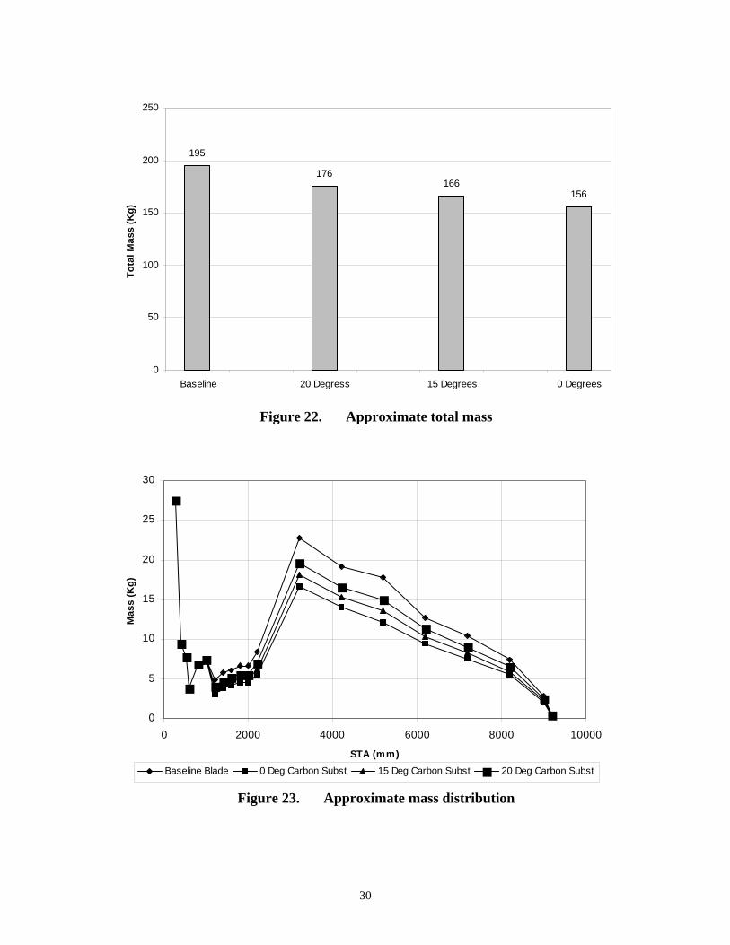
calculations, was assumed to start at station 1000 and end at station 7200. Figure 21 shows the spanwise variation in surface area. Figures 22 and 23 show the resulting weight approximation.
0.00
0.25
0.50
0.75
1.00
1.25
1.50
1.75
2.00
2.25
0 2000 4000 6000 8000 10000
STA (mm)
Are
a (m
^2)
Figure 21. Approximate surface area distribution for the NPS-100 prototype
blade.
30
195
176166
156
0
50
100
150
200
250
Baseline 20 Degress 15 Degrees 0 Degrees
Tota
l Mas
s (K
g)
Figure 22. Approximate total mass
0
5
10
15
20
25
30
0 2000 4000 6000 8000 10000
STA (mm)
Mas
s (K
g)
Baseline Blade 0 Deg Carbon Subst 15 Deg Carbon Subst 20 Deg Carbon Subst
Figure 23. Approximate mass distribution

31
3.2 Stiffness Results Based on the assumption that an equivalent value of the spar cap axial stiffness coefficient would yield satisfactory results, models I through IV were developed following the information shown in Figure 20. At this stage the main goal was to obtain a flapwise bending stiffness (EI) for models II through IV that was the same as the baseline. The results obtained by the finite element analysis for the baseline were compared with preliminary unpublished data that were provided by Mike Zuteck, of MDZ Consulting. As indicated in the following section, Mike Zuteck’s estimated stiffness and the finite element determined stiffness are in good agreement in the flapwise direction. The models were also used to evaluate the edgewise and torsional stiffness of the blade. For this set of analyses the blade was treated as a cantilever beam with all of the model degrees of freedom constrained at the root section. 3.2.1 Flapwise Rigidity To study the flapwise rigidity, two 250 lb loads were applied to the tip of the blade as shown in Figure 24.
Figure 24. Application of a 500 lb flapwise tip load From the deformed results the vertical deflection was recorded and both the bending angle and bending rate per unit length were calculated following the same approach used by McKrittick, Cairns and Mandell in Reference 15 described as follows. The leading and trailing edge nodes were selected for the angle calculations. The bending stiffness is then approximated using:
dzdMEI/θ
= (5)
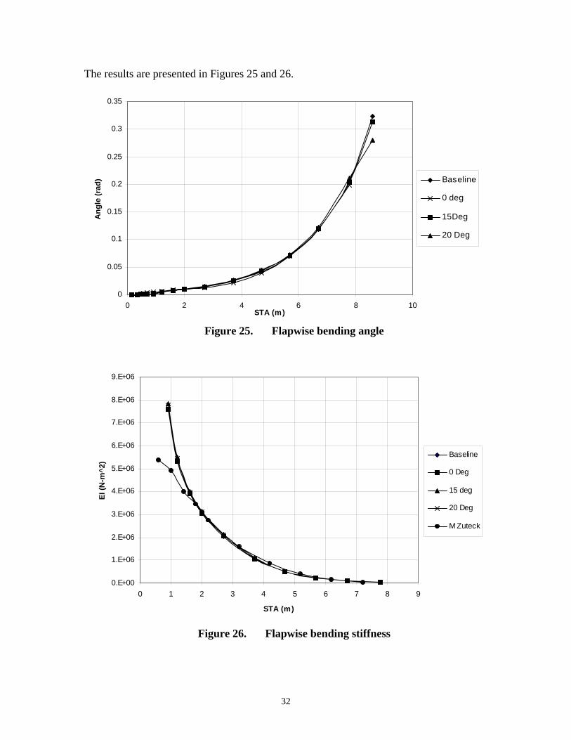
32
The results are presented in Figures 25 and 26.
0
0.05
0.1
0.15
0.2
0.25
0.3
0.35
0 2 4 6 8 10STA (m)
Ang
le (r
ad) Baseline
0 deg
15Deg
20 Deg
Figure 25. Flapwise bending angle
0.E+00
1.E+06
2.E+06
3.E+06
4.E+06
5.E+06
6.E+06
7.E+06
8.E+06
9.E+06
0 1 2 3 4 5 6 7 8 9
STA (m)
EI (N
-m^2
)
Baseline
0 Deg
15 deg
20 Deg
M Zuteck
Figure 26. Flapwise bending stiffness
33
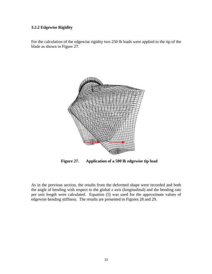
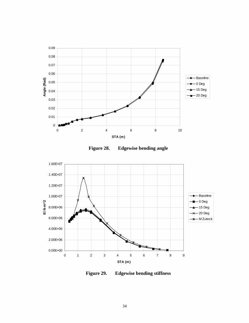
3.2.2 Edgewise Rigidity For the calculation of the edgewise rigidity two 250 lb loads were applied to the tip of the blade as shown in Figure 27.
Figure 27. Application of a 500 lb edgewise tip load As in the previous section, the results from the deformed shape were recorded and both the angle of bending with respect to the global z axis (longitudinal) and the bending rate per unit length were calculated. Equation (5) was used for the approximate values of edgewise bending stiffness. The results are presented in Figures 28 and 29.
34
0
0.01
0.02
0.03
0.04
0.05
0.06
0.07
0.08
0.09
0 2 4 6 8 10
STA (m)
Ang
le (R
ad) Baseline
0 Deg
15 Deg
20 Deg
Figure 28. Edgewise bending angle
0.00E+00
2.00E+06
4.00E+06
6.00E+06
8.00E+06
1.00E+07
1.20E+07
1.40E+07
1.60E+07
0 1 2 3 4 5 6 7 8 9
STA (m)
EI N
-m^2
Baseline
0 Deg
15 Deg
20 Deg
M Zuteck
Figure 29. Edgewise bending stiffness
35
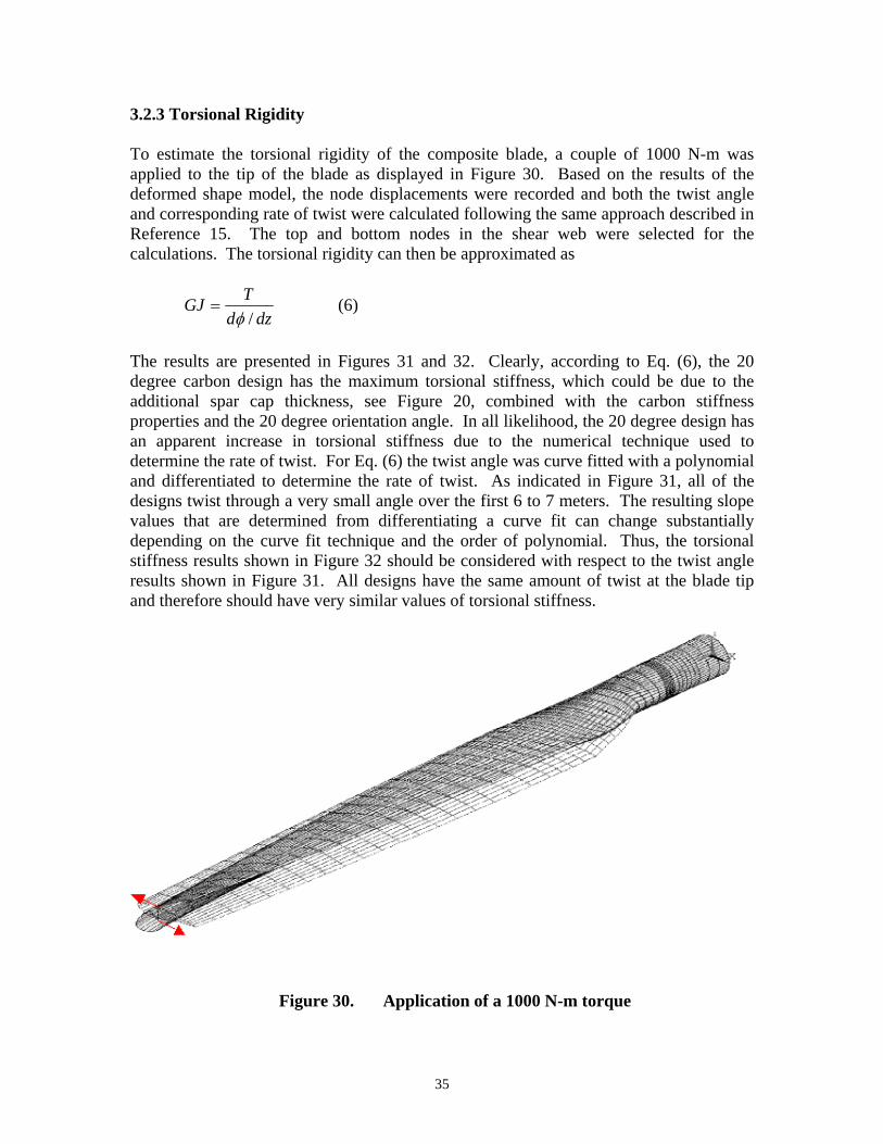
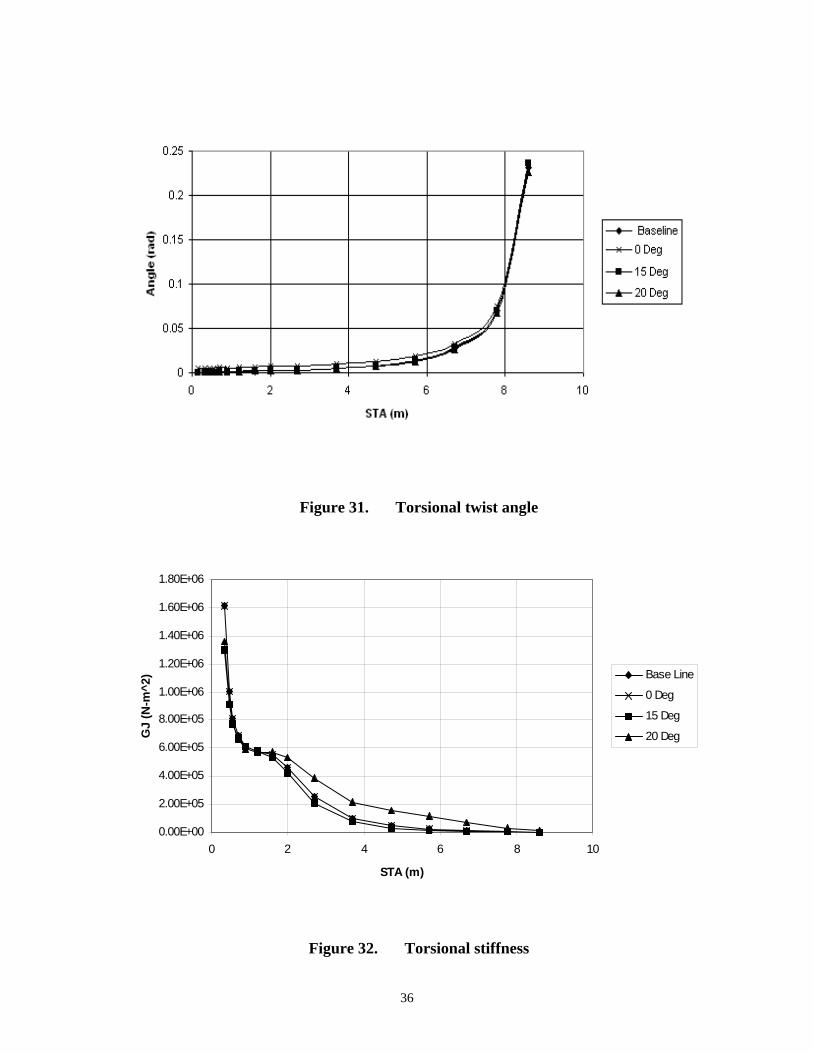
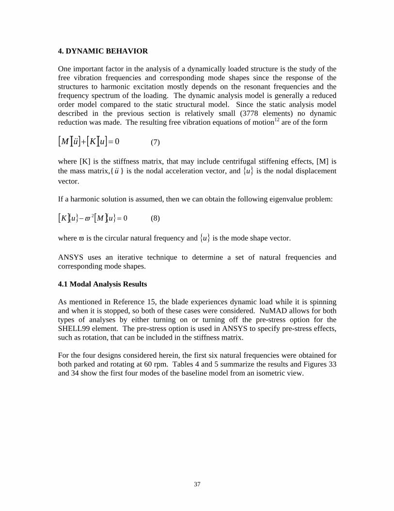
3.2.3 Torsional Rigidity To estimate the torsional rigidity of the composite blade, a couple of 1000 N-m was applied to the tip of the blade as displayed in Figure 30. Based on the results of the deformed shape model, the node displacements were recorded and both the twist angle and corresponding rate of twist were calculated following the same approach described in Reference 15. The top and bottom nodes in the shear web were selected for the calculations. The torsional rigidity can then be approximated as
dzdTGJ/φ
= (6)
The results are presented in Figures 31 and 32. Clearly, according to Eq. (6), the 20 degree carbon design has the maximum torsional stiffness, which could be due to the additional spar cap thickness, see Figure 20, combined with the carbon stiffness properties and the 20 degree orientation angle. In all likelihood, the 20 degree design has an apparent increase in torsional stiffness due to the numerical technique used to determine the rate of twist. For Eq. (6) the twist angle was curve fitted with a polynomial and differentiated to determine the rate of twist. As indicated in Figure 31, all of the designs twist through a very small angle over the first 6 to 7 meters. The resulting slope values that are determined from differentiating a curve fit can change substantially depending on the curve fit technique and the order of polynomial. Thus, the torsional stiffness results shown in Figure 32 should be considered with respect to the twist angle results shown in Figure 31. All designs have the same amount of twist at the blade tip and therefore should have very similar values of torsional stiffness.
Figure 30. Application of a 1000 N-m torque
36
Figure 31. Torsional twist angle
0.00E+00
2.00E+05
4.00E+05
6.00E+05
8.00E+05
1.00E+06
1.20E+06
1.40E+06
1.60E+06
1.80E+06
0 2 4 6 8 10
STA (m)
GJ
(N-m
^2) Base Line
0 Deg
15 Deg
20 Deg
Figure 32. Torsional stiffness
37
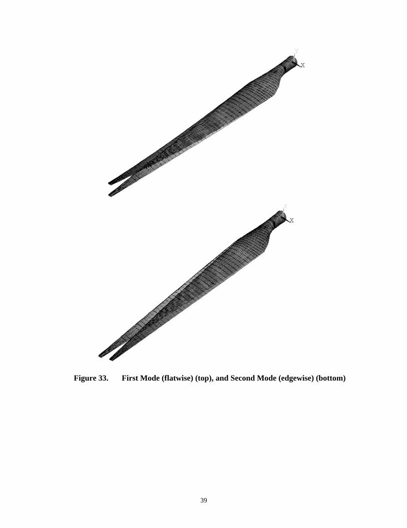
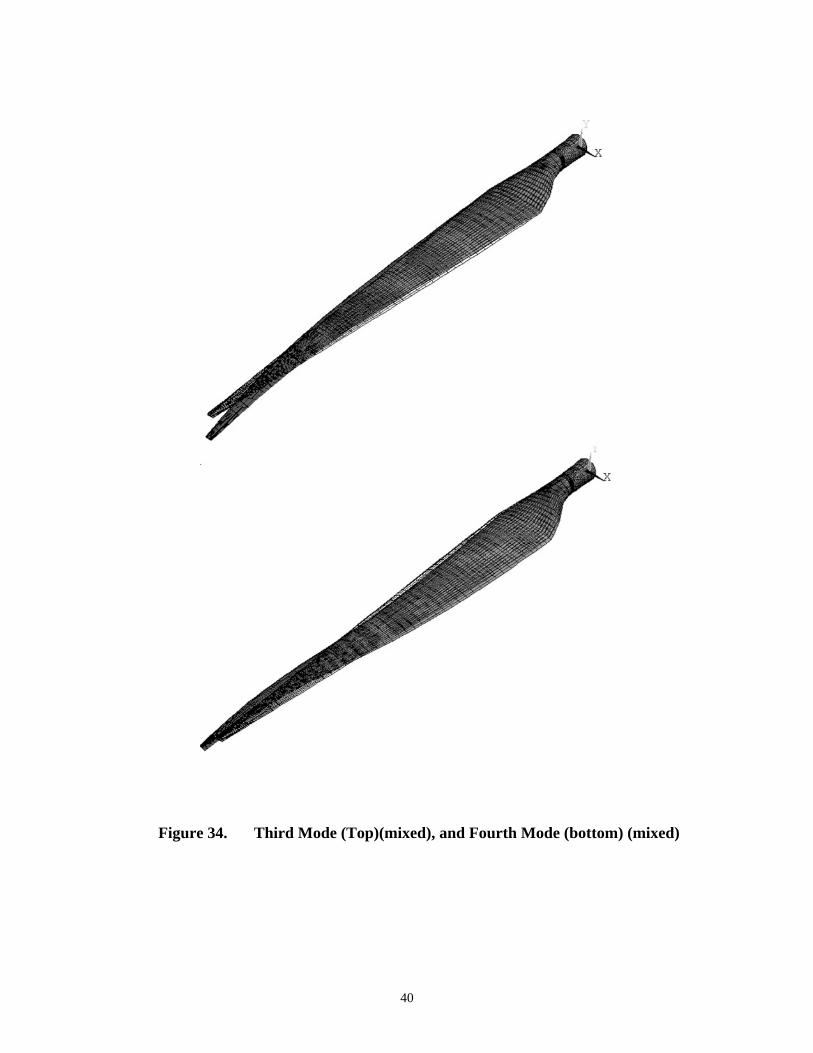
4. DYNAMIC BEHAVIOR One important factor in the analysis of a dynamically loaded structure is the study of the free vibration frequencies and corresponding mode shapes since the response of the structures to harmonic excitation mostly depends on the resonant frequencies and the frequency spectrum of the loading. The dynamic analysis model is generally a reduced order model compared to the static structural model. Since the static analysis model described in the previous section is relatively small (3778 elements) no dynamic reduction was made. The resulting free vibration equations of motion12 are of the form [ ][ ] [ ][ ] 0=+ uKuM && (7) where [K] is the stiffness matrix, that may include centrifugal stiffening effects, [M] is the mass matrix,{u&& } is the nodal acceleration vector, and { }u is the nodal displacement vector. If a harmonic solution is assumed, then we can obtain the following eigenvalue problem: [ ]{ } [ ]{ } 02 =− uMuK ϖ (8) where ϖ is the circular natural frequency and { }u is the mode shape vector. ANSYS uses an iterative technique to determine a set of natural frequencies and corresponding mode shapes. 4.1 Modal Analysis Results As mentioned in Reference 15, the blade experiences dynamic load while it is spinning and when it is stopped, so both of these cases were considered. NuMAD allows for both types of analyses by either turning on or turning off the pre-stress option for the SHELL99 element. The pre-stress option is used in ANSYS to specify pre-stress effects, such as rotation, that can be included in the stiffness matrix. For the four designs considered herein, the first six natural frequencies were obtained for both parked and rotating at 60 rpm. Tables 4 and 5 summarize the results and Figures 33 and 34 show the first four modes of the baseline model from an isometric view.
38
Parked
1st. 2nd 3rd 4th 5th 6th Hz Hz Hz Hz Hz Hz
Base Line 4.524 7.13 12.265 22.434 24.583 34.824 (flapwise) (edgewise) (flapwise) (mixed) (mixed) (mixed)
0 Degree 5.452 8.326 14.8 26.421 29.059 38.329 (flapwise) (edgewise) (flapwise) (mixed) (mixed) (mixed)
15 Degree 5.099 7.958 14.004 25.309 27.652 37.538 (flapwise) (edgewise) (flapwise) (mixed) (mixed) (mixed)
20 Degree 4.839 7.664 13.285 24.239 26.481 36.84 (flapwise) (edgewise) (flapwise) (mixed) (mixed) (mixed)
Table 3. First six natural frequencies in parked condition Operating at 60RPM
1st. 2nd 3rd 4th 5th 6th Hz Hz Hz Hz Hz Hz
Base Line 4.707 7.222 12.478 22.597 24.715 35.016 (flapwise) (edgewise) (flapwise) (mixed) (mixed) (mixed)
0 Degree 5.6 8.407 14.975 26.561 29.185 38.49 (flapwise) (edgewise) (flapwise) (mixed) (mixed) (mixed)
15 Degree 5.257 8.042 14.19 25.451 27.791 37.706 (flapwise) (edgewise) (flapwise) (mixed) (mixed) (mixed)
20 Degree 5.007 7.75 13.482 24.388 26.63 37.017 (flapwise) (edgewise) (flapwise) (mixed) (mixed) (mixed)
Table 4. First six natural frequencies operating at 60 rpm
39
Figure 33. First Mode (flatwise) (top), and Second Mode (edgewise) (bottom)
40
Figure 34. Third Mode (Top)(mixed), and Fourth Mode (bottom) (mixed)
41
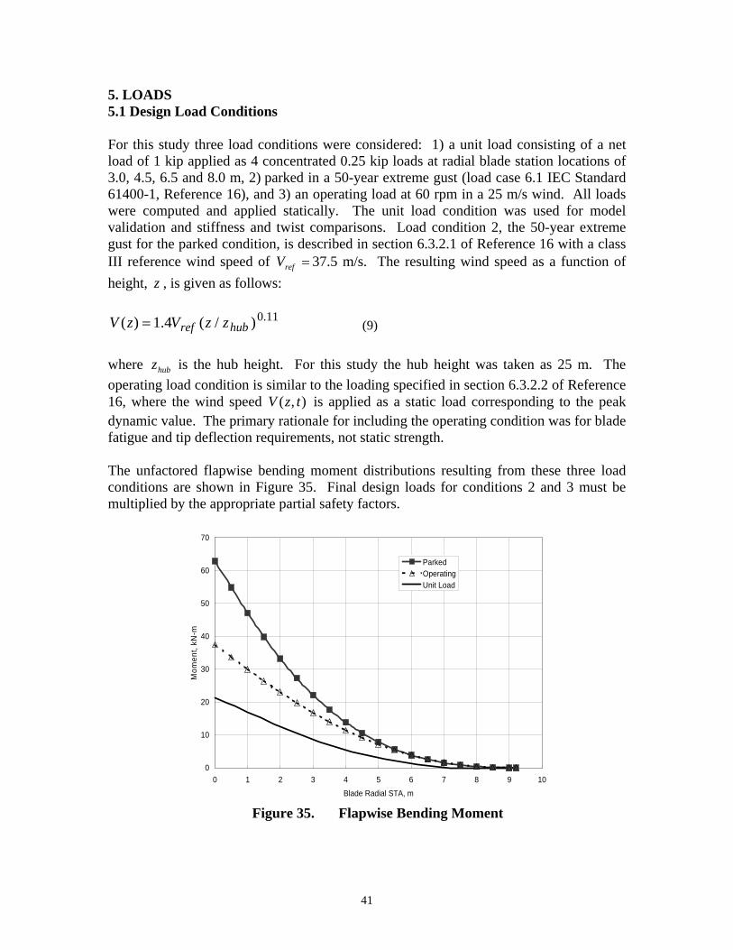
5. LOADS 5.1 Design Load Conditions For this study three load conditions were considered: 1) a unit load consisting of a net load of 1 kip applied as 4 concentrated 0.25 kip loads at radial blade station locations of 3.0, 4.5, 6.5 and 8.0 m, 2) parked in a 50-year extreme gust (load case 6.1 IEC Standard 61400-1, Reference 16), and 3) an operating load at 60 rpm in a 25 m/s wind. All loads were computed and applied statically. The unit load condition was used for model validation and stiffness and twist comparisons. Load condition 2, the 50-year extreme gust for the parked condition, is described in section 6.3.2.1 of Reference 16 with a class III reference wind speed of =refV 37.5 m/s. The resulting wind speed as a function of height, z , is given as follows:
11.0)/(4.1)( hubref zzVzV = (9)
where hubz is the hub height. For this study the hub height was taken as 25 m. The operating load condition is similar to the loading specified in section 6.3.2.2 of Reference 16, where the wind speed ),( tzV is applied as a static load corresponding to the peak dynamic value. The primary rationale for including the operating condition was for blade fatigue and tip deflection requirements, not static strength. The unfactored flapwise bending moment distributions resulting from these three load conditions are shown in Figure 35. Final design loads for conditions 2 and 3 must be multiplied by the appropriate partial safety factors.
0
10
20
30
40
50
60
70
0 1 2 3 4 5 6 7 8 9 10Blade Radial STA, m
Mom
ent,
kN-m
ParkedOperatingUnit Load
Figure 35. Flapwise Bending Moment
42
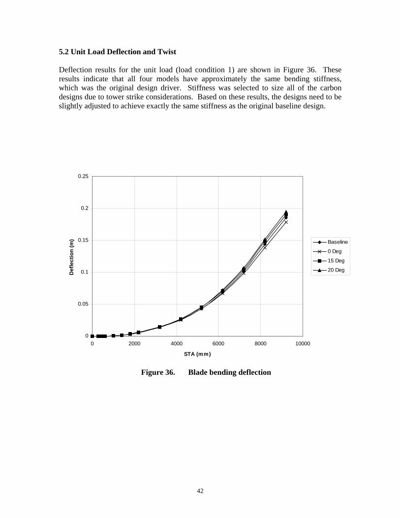
5.2 Unit Load Deflection and Twist Deflection results for the unit load (load condition 1) are shown in Figure 36. These results indicate that all four models have approximately the same bending stiffness, which was the original design driver. Stiffness was selected to size all of the carbon designs due to tower strike considerations. Based on these results, the designs need to be slightly adjusted to achieve exactly the same stiffness as the original baseline design.
0
0.05
0.1
0.15
0.2
0.25
0 2000 4000 6000 8000 10000
STA (mm)
Def
lect
ion
(m) Baseline
0 Deg
15 Deg
20 Deg
Figure 36. Blade bending deflection
43
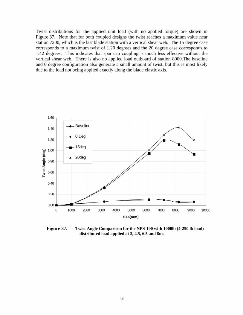
Twist distributions for the applied unit load (with no applied torque) are shown in Figure 37. Note that for both coupled designs the twist reaches a maximum value near station 7200, which is the last blade station with a vertical shear web. The 15 degree case corresponds to a maximum twist of 1.20 degrees and the 20 degree case corresponds to 1.42 degrees. This indicates that spar cap coupling is much less effective without the vertical shear web. There is also no applied load outboard of station 8000.The baseline and 0 degree configuration also generate a small amount of twist, but this is most likely due to the load not being applied exactly along the blade elastic axis.
0.00
0.20
0.40
0.60
0.80
1.00
1.20
1.40
1.60
0 1000 2000 3000 4000 5000 6000 7000 8000 9000 10000
STA(mm)
Twis
t Ang
le (d
eg)
Baseline
0 Deg
15deg
20deg
Figure 37. Twist Angle Comparison for the NPS-100 with 1000lb (4-250 lb load)
distributed load applied at 3, 4.5, 6.5 and 8m.
44
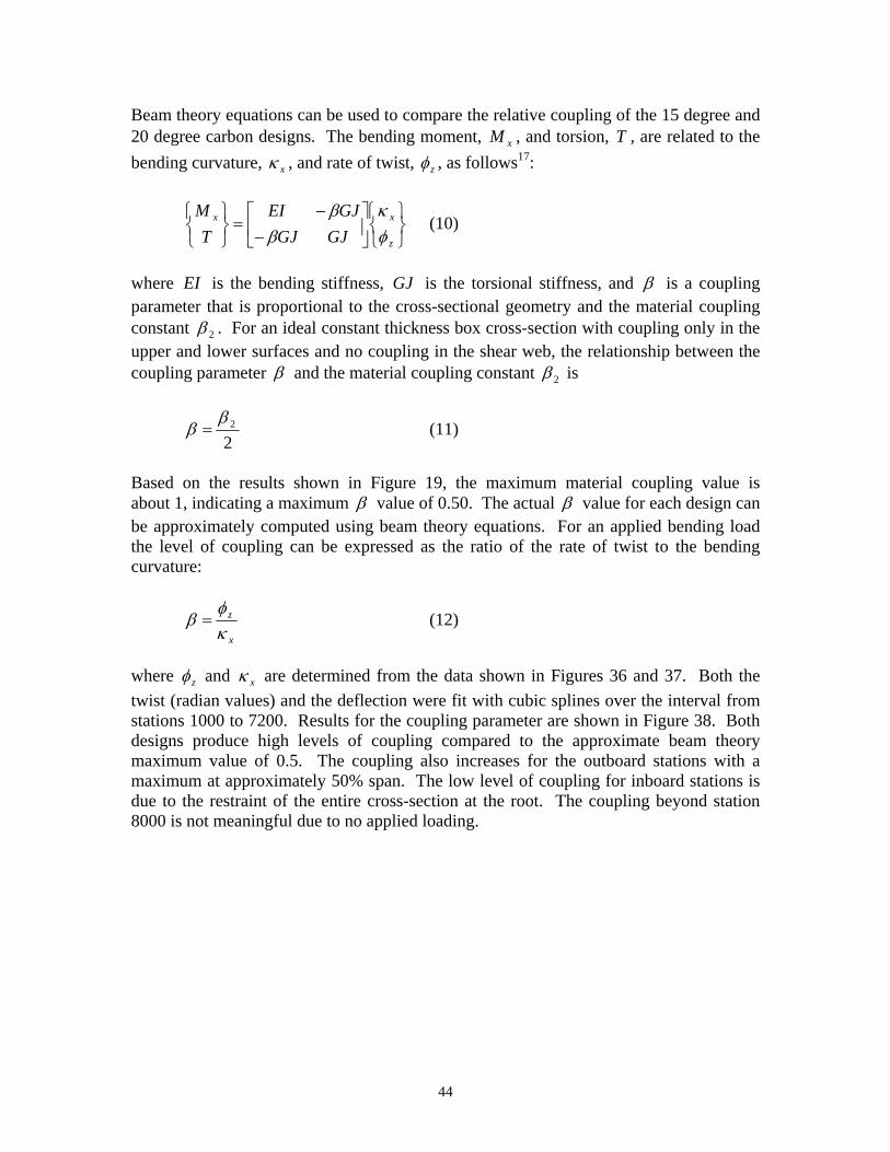
Beam theory equations can be used to compare the relative coupling of the 15 degree and 20 degree carbon designs. The bending moment, xM , and torsion, T , are related to the bending curvature, xκ , and rate of twist, zφ , as follows17:
⎭⎬⎫
⎩⎨⎧
⎥⎦
⎤⎢⎣
⎡−
−=
⎭⎬⎫
⎩⎨⎧
z
xx
GJGJGJEI
TM
φκ
ββ
(10)
where EI is the bending stiffness, GJ is the torsional stiffness, and β is a coupling parameter that is proportional to the cross-sectional geometry and the material coupling constant 2β . For an ideal constant thickness box cross-section with coupling only in the upper and lower surfaces and no coupling in the shear web, the relationship between the coupling parameter β and the material coupling constant 2β is
22β
β = (11)
Based on the results shown in Figure 19, the maximum material coupling value is about 1, indicating a maximum β value of 0.50. The actual β value for each design can be approximately computed using beam theory equations. For an applied bending load the level of coupling can be expressed as the ratio of the rate of twist to the bending curvature:
x
z
κφ
β = (12)
where zφ and xκ are determined from the data shown in Figures 36 and 37. Both the twist (radian values) and the deflection were fit with cubic splines over the interval from stations 1000 to 7200. Results for the coupling parameter are shown in Figure 38. Both designs produce high levels of coupling compared to the approximate beam theory maximum value of 0.5. The coupling also increases for the outboard stations with a maximum at approximately 50% span. The low level of coupling for inboard stations is due to the restraint of the entire cross-section at the root. The coupling beyond station 8000 is not meaningful due to no applied loading.
45
0.30
0.35
0.40
0.45
0.50
0.55
0.60
0.65
0.70
0 1 2 3 4 5 6 7 8Blade Radial STA, m
Cou
plin
g P
aram
eter
Carbon 15 degrees
Carbon 20 degrees
Figure 38. Twist-coupling parameter β
46
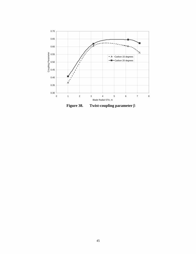
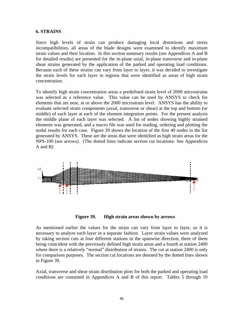
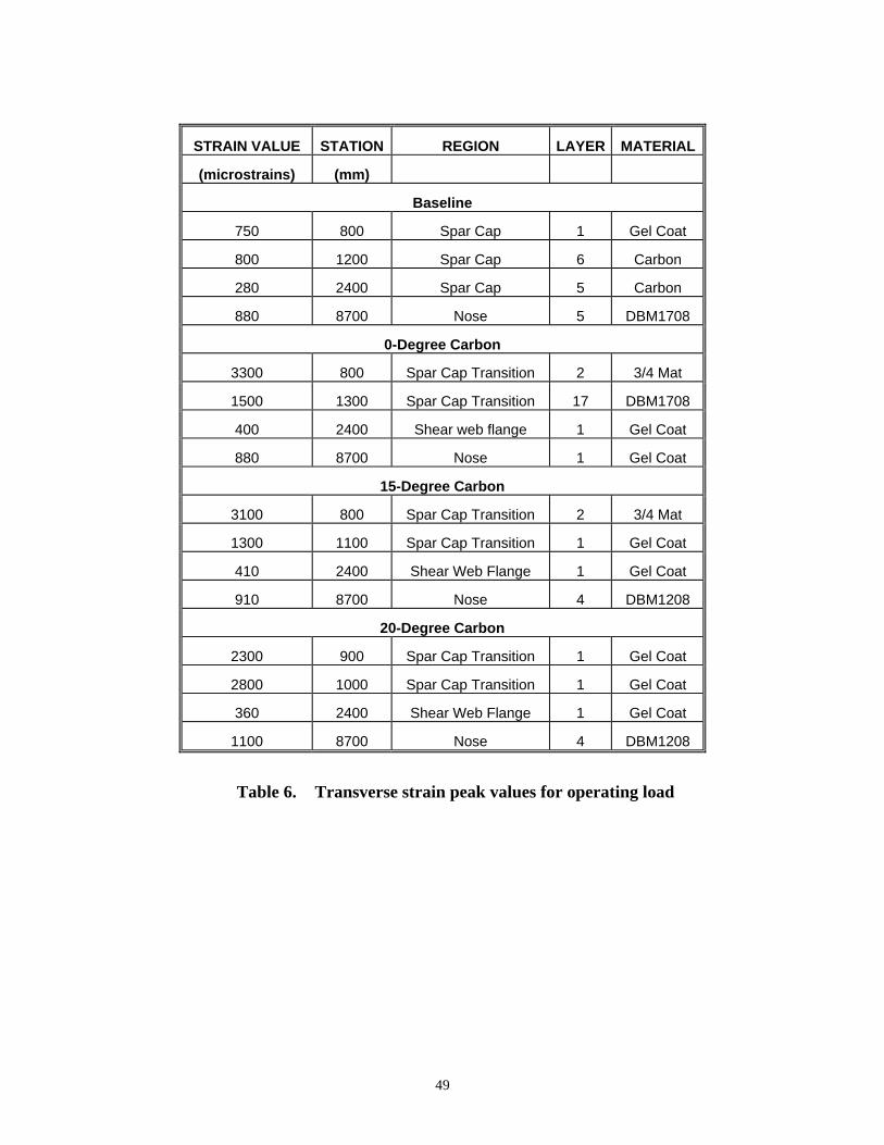
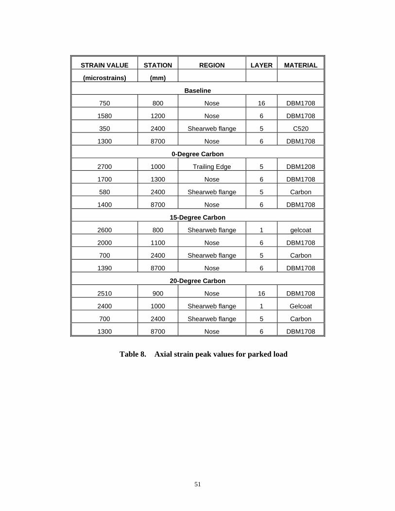
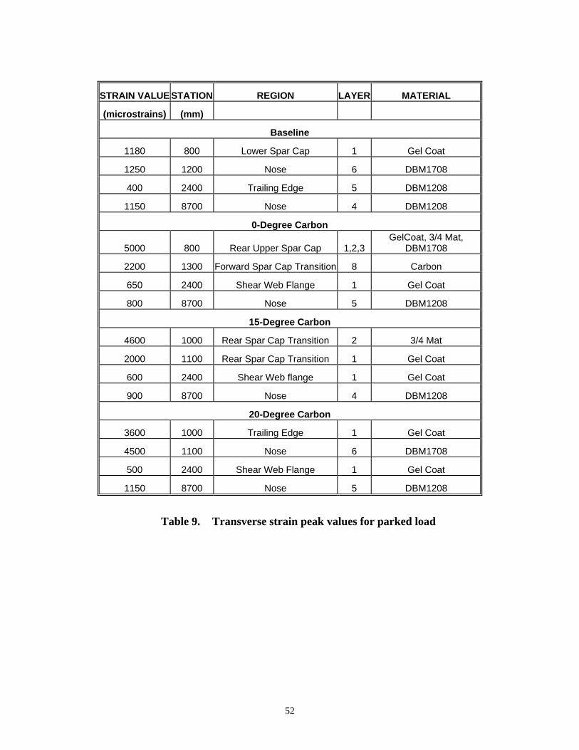
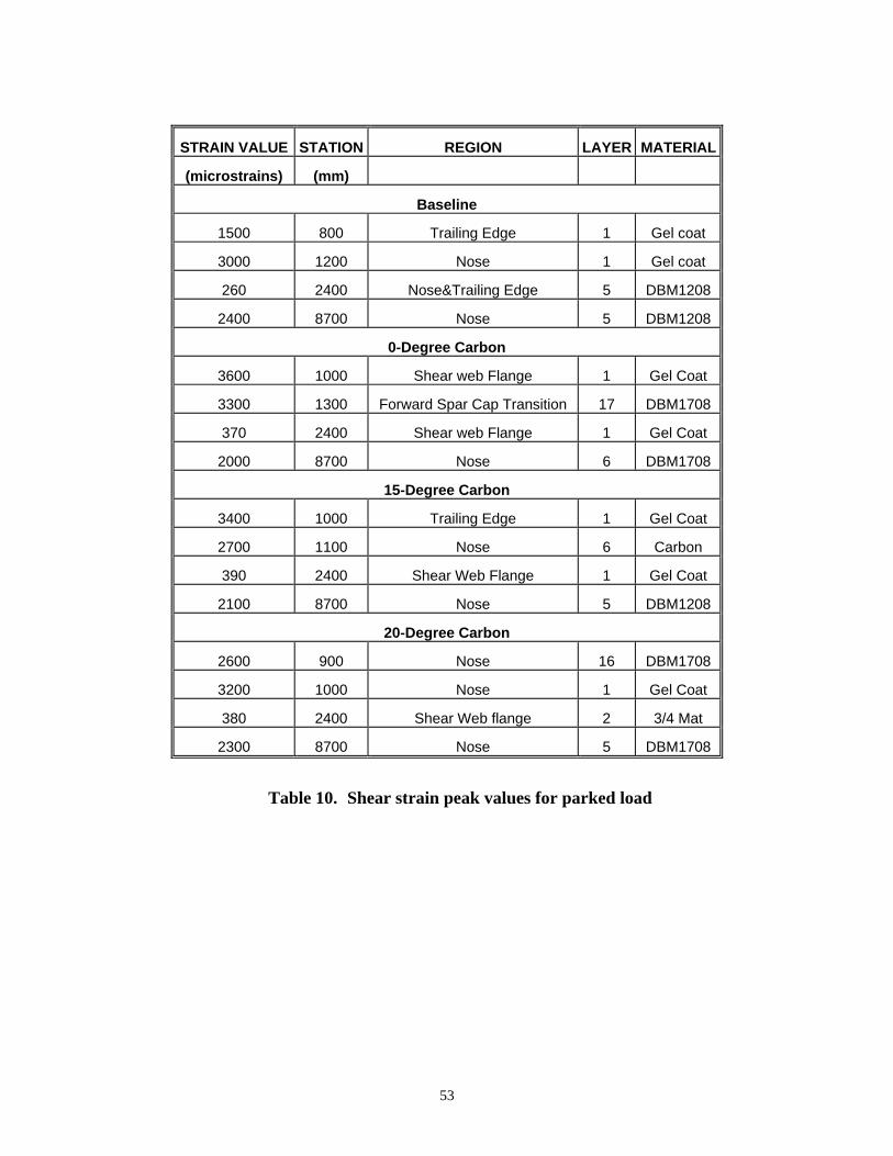
6. STRAINS Since high levels of strain can produce damaging local distortions and stress incompatibilities, all areas of the blade designs were examined to identify maximum strain values and their location. In this section summary results (see Appendices A and B for detailed results) are presented for the in-plane axial, in-plane transverse and in-plane shear strains generated by the application of the parked and operating load conditions. Because each of these strains can vary from layer to layer, it was decided to investigate the strain levels for each layer in regions that were identified as areas of high strain concentration. To identify high strain concentration areas a predefined strain level of 2000 microstrains was selected as a reference value. This value can be used by ANSYS to check for elements that are near, at or above the 2000 microstrain level. ANSYS has the ability to evaluate selected strain components (axial, transverse or shear) at the top and bottom (or middle) of each layer at each of the element integration points. For the present analysis the middle plane of each layer was selected. A list of nodes showing highly strained elements was generated, and a macro file was used for reading, ordering and plotting the nodal results for each case. Figure 39 shows the location of the first 40 nodes in the list generated by ANSYS. These are the areas that were identified as high strain areas for the NPS-100 (see arrows). (The dotted lines indicate section cut locations- See Appendices A and B)
Figure 39. High strain areas shown by arrows As mentioned earlier the values for the strain can vary from layer to layer, so it is necessary to analyze each layer in a separate fashion. Layer strain values were analyzed by taking section cuts at four different stations in the spanwise direction, three of them being coincident with the previously defined high strain areas and a fourth at station 2400 where there is a relatively “normal” distribution of strains. The cut at station 2400 is only for comparison purposes. The section cut locations are denoted by the dotted lines shown in Figure 39. Axial, transverse and shear strain distribution plots for both the parked and operating load conditions are contained in Appendices A and B of this report. Tables 5 through 10

47
summarize the strain peak values, corresponding blade station and layer for each of the strain distribution plots presented in the Appendices.
48
STRAIN VALUE STATION REGION LAYER MATERIAL
(microstrains) (mm)
Baseline
550 800 Nose 16 DBM1708
900 1200 Nose 6 Carbon
280 2400 Shear Web Flange 5 Carbon
1050 8700 Nose 6 DBM1708
0-Degree Carbon
1750 1000 Shear web Flange 1 Gel Coat
1100 1300 Forward Spar Cap Transition 17 DBM1708
470 2400 Shear web Flange 1 Gel Coat
1600 8700 Nose 6 DBM1708
15-Degree Carbon
1210 1000 Trailing Edge 1 Gel Coat
1220 1100 Nose 6 DBM1708
550 2400 Shear Web Flange 1 Gel Coat
1550 8700 Nose 5 DBM1208
20-Degree Carbon
1780 900 Nose 16 DBM1708
1200 1000 Nose 1 Gel Coat
550 2400 Shear Web flange 2 3/4 Mat
1410 8700 Nose 5 DBM1208
Table 5. Axial strain peak values for operating load
49
STRAIN VALUE STATION REGION LAYER MATERIAL
(microstrains) (mm)
Baseline
750 800 Spar Cap 1 Gel Coat
800 1200 Spar Cap 6 Carbon
280 2400 Spar Cap 5 Carbon
880 8700 Nose 5 DBM1708
0-Degree Carbon
3300 800 Spar Cap Transition 2 3/4 Mat
1500 1300 Spar Cap Transition 17 DBM1708
400 2400 Shear web flange 1 Gel Coat
880 8700 Nose 1 Gel Coat
15-Degree Carbon
3100 800 Spar Cap Transition 2 3/4 Mat
1300 1100 Spar Cap Transition 1 Gel Coat
410 2400 Shear Web Flange 1 Gel Coat
910 8700 Nose 4 DBM1208
20-Degree Carbon
2300 900 Spar Cap Transition 1 Gel Coat
2800 1000 Spar Cap Transition 1 Gel Coat
360 2400 Shear Web Flange 1 Gel Coat
1100 8700 Nose 4 DBM1208
Table 6. Transverse strain peak values for operating load

50
STRAIN VALUE STATION REGION LAYER MATERIAL
(microstrains) (mm)
Baseline
890 800 Trailing edge 1 Gel Coat
1800 1200 Nose 1 Gel Coat
250 2400 Nose 6 DBM1208
1580 8700 Nose 4 DBM1208
0-Degree Carbon
2400 1000 Rear Spar Cap 1 Gel Coat
2300 1300 Fwd Spar Cap 17 DBM1208
300 2400 Nose 3 DBM1708
2300 8700 Nose 6 DBM1708
15-Degree Carbon
2300 1000 Rear Spar Cap 1 Gel Coat
1900 1100 Nose 6 DBM1708
310 2400 Nose 7 DBM1708
2300 8700 Nose 5 DBM1208
20-Degree Carbon
1700 900 Nose 16 DBM1708
2300 1000 Nose 1 Gel Coat
310 2400 Nose 7 DBM1708
2400 8700 Nose 5 DBM1208
Table 7. Shear strain peak values for operating load
51
STRAIN VALUE STATION REGION LAYER MATERIAL
(microstrains) (mm)
Baseline
750 800 Nose 16 DBM1708
1580 1200 Nose 6 DBM1708
350 2400 Shearweb flange 5 C520
1300 8700 Nose 6 DBM1708
0-Degree Carbon
2700 1000 Trailing Edge 5 DBM1208
1700 1300 Nose 6 DBM1708
580 2400 Shearweb flange 5 Carbon
1400 8700 Nose 6 DBM1708
15-Degree Carbon
2600 800 Shearweb flange 1 gelcoat
2000 1100 Nose 6 DBM1708
700 2400 Shearweb flange 5 Carbon
1390 8700 Nose 6 DBM1708
20-Degree Carbon
2510 900 Nose 16 DBM1708
2400 1000 Shearweb flange 1 Gelcoat
700 2400 Shearweb flange 5 Carbon
1300 8700 Nose 6 DBM1708
Table 8. Axial strain peak values for parked load
52
STRAIN VALUE STATION REGION LAYER MATERIAL
(microstrains) (mm)
Baseline
1180 800 Lower Spar Cap 1 Gel Coat
1250 1200 Nose 6 DBM1708
400 2400 Trailing Edge 5 DBM1208
1150 8700 Nose 4 DBM1208
0-Degree Carbon
5000 800 Rear Upper Spar Cap 1,2,3 GelCoat, 3/4 Mat,
DBM1708
2200 1300 Forward Spar Cap Transition 8 Carbon
650 2400 Shear Web Flange 1 Gel Coat
800 8700 Nose 5 DBM1208
15-Degree Carbon
4600 1000 Rear Spar Cap Transition 2 3/4 Mat
2000 1100 Rear Spar Cap Transition 1 Gel Coat
600 2400 Shear Web flange 1 Gel Coat
900 8700 Nose 4 DBM1208
20-Degree Carbon
3600 1000 Trailing Edge 1 Gel Coat
4500 1100 Nose 6 DBM1708
500 2400 Shear Web Flange 1 Gel Coat
1150 8700 Nose 5 DBM1208
Table 9. Transverse strain peak values for parked load
53
STRAIN VALUE STATION REGION LAYER MATERIAL
(microstrains) (mm)
Baseline
1500 800 Trailing Edge 1 Gel coat
3000 1200 Nose 1 Gel coat
260 2400 Nose&Trailing Edge 5 DBM1208
2400 8700 Nose 5 DBM1208
0-Degree Carbon
3600 1000 Shear web Flange 1 Gel Coat
3300 1300 Forward Spar Cap Transition 17 DBM1708
370 2400 Shear web Flange 1 Gel Coat
2000 8700 Nose 6 DBM1708
15-Degree Carbon
3400 1000 Trailing Edge 1 Gel Coat
2700 1100 Nose 6 Carbon
390 2400 Shear Web Flange 1 Gel Coat
2100 8700 Nose 5 DBM1208
20-Degree Carbon
2600 900 Nose 16 DBM1708
3200 1000 Nose 1 Gel Coat
380 2400 Shear Web flange 2 3/4 Mat
2300 8700 Nose 5 DBM1708
Table 10. Shear strain peak values for parked load
54
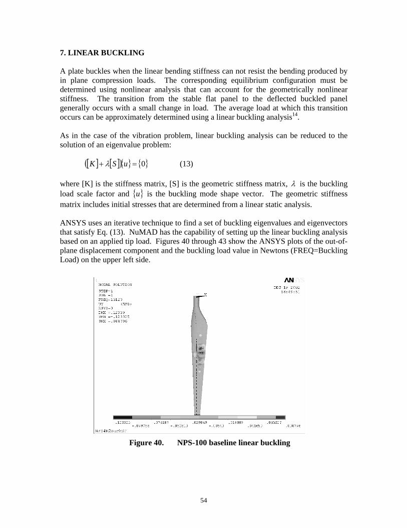
7. LINEAR BUCKLING A plate buckles when the linear bending stiffness can not resist the bending produced by in plane compression loads. The corresponding equilibrium configuration must be determined using nonlinear analysis that can account for the geometrically nonlinear stiffness. The transition from the stable flat panel to the deflected buckled panel generally occurs with a small change in load. The average load at which this transition occurs can be approximately determined using a linear buckling analysis14. As in the case of the vibration problem, linear buckling analysis can be reduced to the solution of an eigenvalue problem:
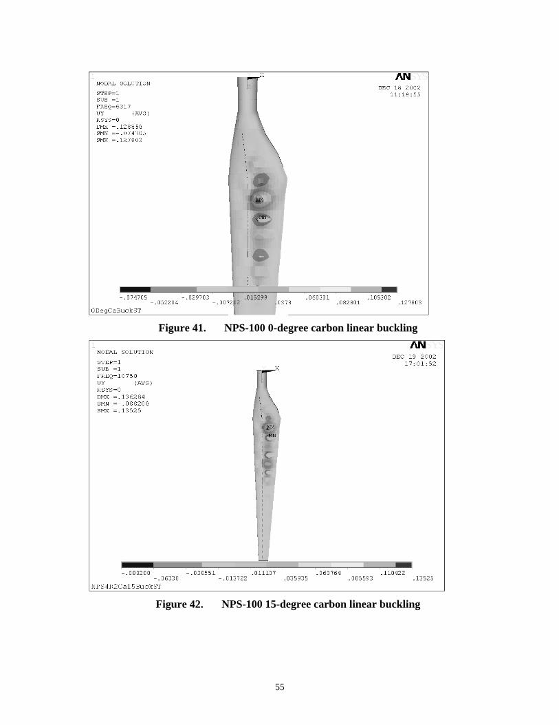
[ ] [ ]( ){ } { }0=+ uSK λ (13) where [K] is the stiffness matrix, [S] is the geometric stiffness matrix, λ is the buckling load scale factor and { }u is the buckling mode shape vector. The geometric stiffness matrix includes initial stresses that are determined from a linear static analysis. ANSYS uses an iterative technique to find a set of buckling eigenvalues and eigenvectors that satisfy Eq. (13). NuMAD has the capability of setting up the linear buckling analysis based on an applied tip load. Figures 40 through 43 show the ANSYS plots of the out-of-plane displacement component and the buckling load value in Newtons (FREQ=Buckling Load) on the upper left side.
Figure 40. NPS-100 baseline linear buckling
55
Figure 41. NPS-100 0-degree carbon linear buckling
Figure 42. NPS-100 15-degree carbon linear buckling

56
Figure 43. NPS-100 20-degree carbon linear buckling
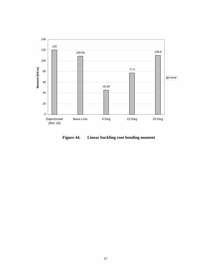
For these analyses, the linear buckling eigenvalues were determined for a unit tip condition, with the tip load applied at the last station with a spar shear web (station 7200). For analysis purposes, the buckling model did not include any blade stations outboard of station 7200. The buckling occurs at approximately 35% span, which is consistent with the test results (31% span) reported in Reference 18. Linear buckling root bending moment (tip buckling load x 7.2 m) results are shown in Figure 44. The load levels required to produce linear buckling are very close for the baseline and 20-degree carbon designs. The 15-degree design buckles at a substantially lower load, which is due the reduced spar cap thickness (63% of the baseline C520 thickness for the 15-degree design compared to 82% of the baseline C520 thickness for the 20-degree design) and corresponding reduced bending stiffness. The baseline linear buckling load of approximately 110 kN-m compares well with the experimental value of 120 kN-m.18
57
120
108.56
45.48
77.4
109.9
0
20
40
60
80
100
120
140
Experimetal(Ref. 18)
Base Line 0 Deg 15 Deg 20 Deg
Mom
ent (
KN
-m)
Linear
Figure 44. Linear buckling root bending moment
58
8. NONLINEAR BUCKLING Nonlinear buckling is a more involved and complex analysis in terms of formulation and solution time than the linear one because higher order strain terms, that are dependent on the displacement, must be included in the equations . This type of analysis requires elements and a solution method that can deal with large deflection geometric nonlinearities. NuMAD does not currently support nonlinear analysis; therefore, all nonlinear buckling analyses were performed directly with ANSYS outside of the NuMAD environment. 8.1 Nonlinear Buckling Analysis The basic method followed was to perform a nonlinear static analysis where the loads were gradually increased until a load level was reached such that the structure became unstable. The overall procedure is summarized as follows:
1. Use one of the models created in NuMAD and copy the master.db ANSYS file to a new directory
2. Open the file and apply the boundary condition at the root and a unit tip load 3. Select a static linear analysis including the pre-stress option "PSTRES”. This is
the same option as described in the vibration problem section. 4. Perform the linear analysis 5. Select a new analysis and choose the Eigen buckling with the Block Lanczos
mode extraction option 6. Use the MXPAND command to expand the modes to be calculated. This basically
means that ANSYS will write the mode shapes to the results file so they are available for the subsequent analysis, i.e. the nonlinear analysis.
7. Perform the linear eigen buckling analysis. 8. Select the "update geometry option" to introduce the imperfections calculated in
the previous analysis. 9. Select a new analysis and choose "static". 10. Select the large deformation effects to be included. 11. Apply the loads.
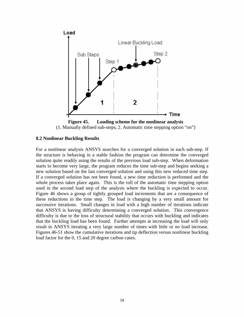
For this analysis a two-load step scheme was utilized. The ANSYS manual defines a load step as a configuration of loads for which a solution is obtained. Each load step is divided into one or more sub-steps where the solutions are calculated. In nonlinear static analysis this allows for the gradual increase of load from a desired level to another in a more or less controlled fashion and the calculation of a solution at each sub-step. The first load step was one that increased the load from zero up to a value near the previously calculated linear buckling load. The second load step increases the load past the expected buckling load. For the second load step the automatic time stepping option of ANSYS was selected to capture as precisely as possible the nonlinear buckling load. Figure 45 shows the loading scheme used for the nonlinear analysis.
59
Figure 45. Loading scheme for the nonlinear analysis
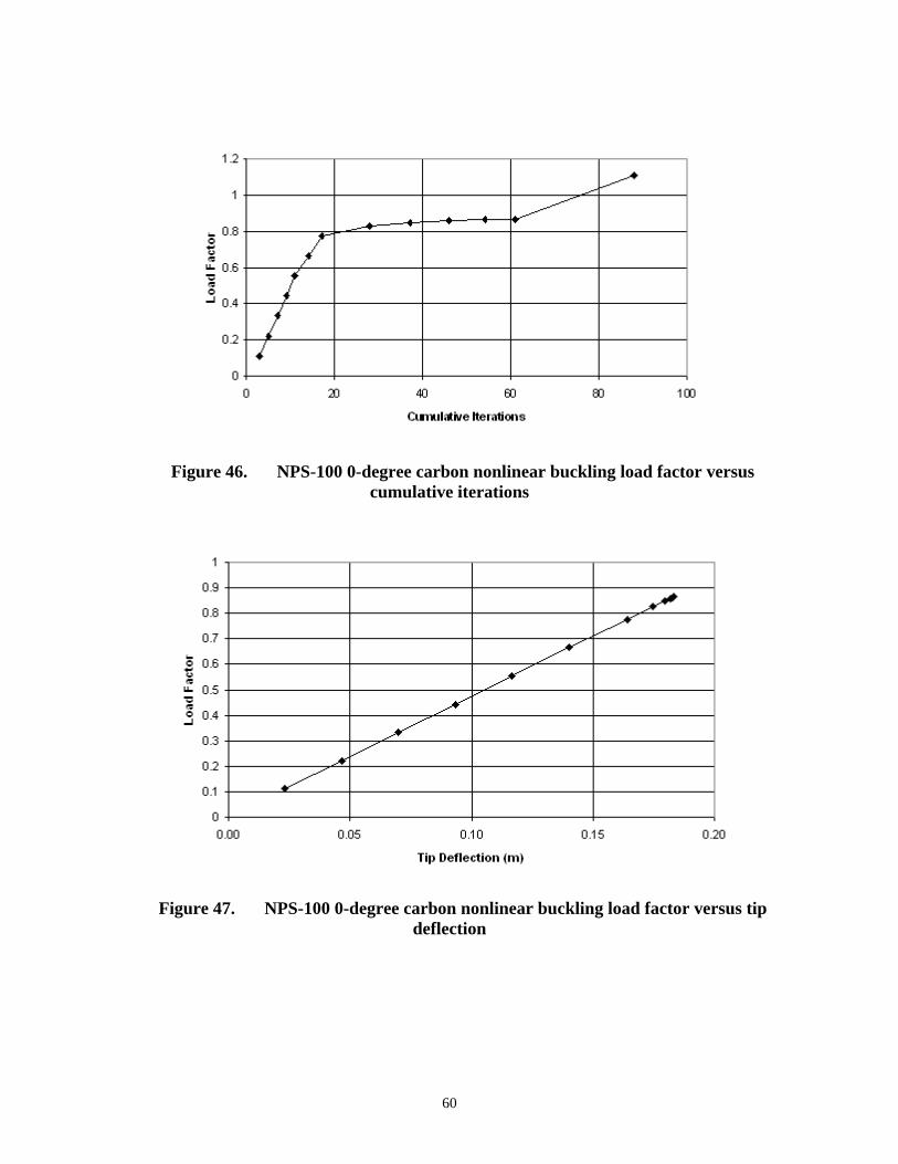
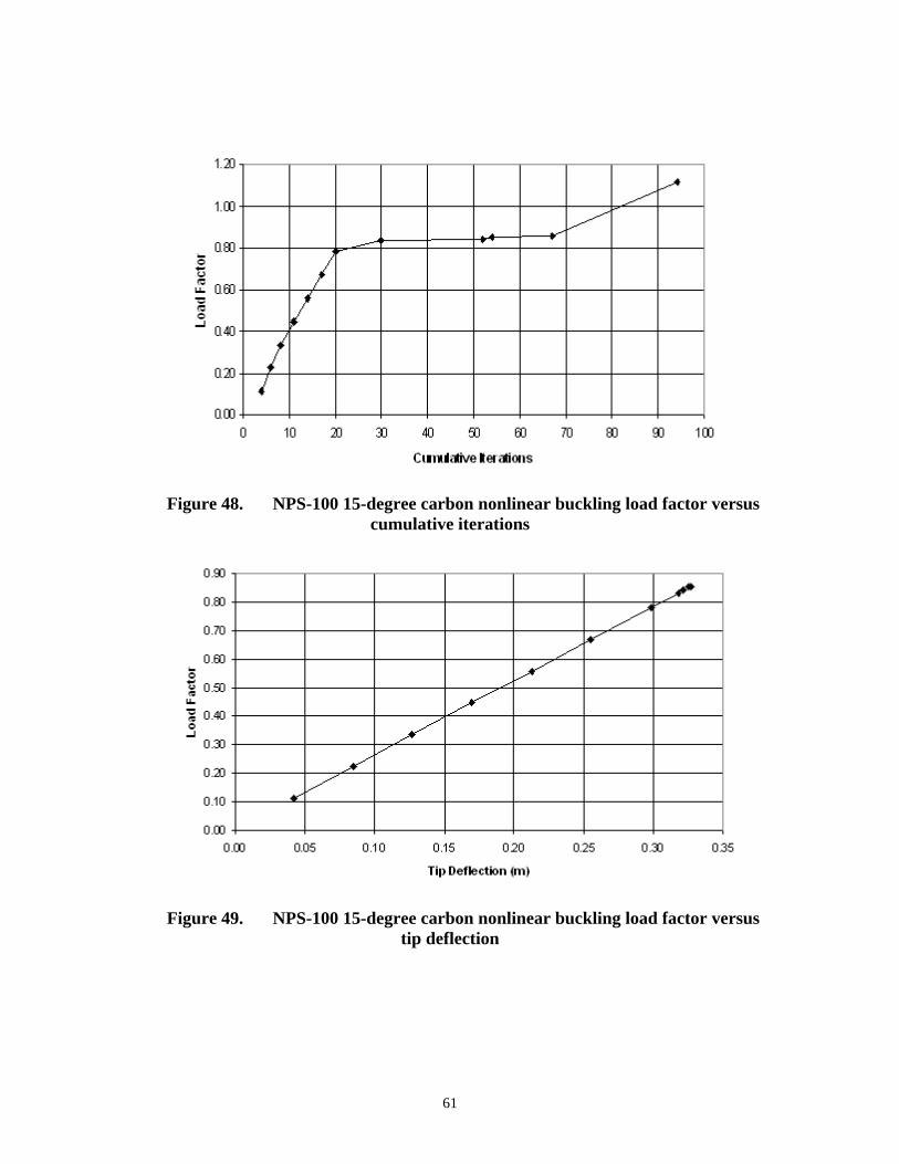
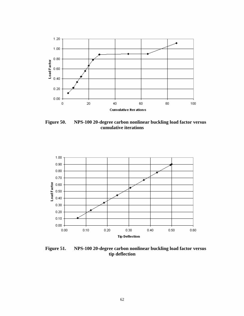
(1. Manually defined sub-steps, 2. Automatic time stepping option “on”) 8.2 Nonlinear Buckling Results For a nonlinear analysis ANSYS searches for a converged solution in each sub-step. If the structure is behaving in a stable fashion the program can determine the converged solution quite readily using the results of the previous load sub-step. When deformation starts to become very large, the program reduces the time sub-step and begins seeking a new solution based on the last converged solution and using this new reduced time step. If a converged solution has not been found, a new time reduction is performed and the whole process takes place again. This is the roll of the automatic time stepping option used in the second load step of the analysis where the buckling is expected to occur. Figure 46 shows a group of tightly grouped load increments that are a consequence of these reductions in the time step. The load is changing by a very small amount for successive iterations. Small changes in load with a high number of iterations indicate that ANSYS is having difficulty determining a converged solution. This convergence difficulty is due to the loss of structural stability that occurs with buckling and indicates that the buckling load has been found. Further attempts at increasing the load will only result in ANSYS iterating a very large number of times with little or no load increase. Figures 46-51 show the cumulative iterations and tip deflection versus nonlinear buckling load factor for the 0, 15 and 20 degree carbon cases.
60
Figure 46. NPS-100 0-degree carbon nonlinear buckling load factor versus
cumulative iterations
Figure 47. NPS-100 0-degree carbon nonlinear buckling load factor versus tip
deflection
61
Figure 48. NPS-100 15-degree carbon nonlinear buckling load factor versus
cumulative iterations
Figure 49. NPS-100 15-degree carbon nonlinear buckling load factor versus
tip deflection
62
Figure 50. NPS-100 20-degree carbon nonlinear buckling load factor versus
cumulative iterations
Figure 51. NPS-100 20-degree carbon nonlinear buckling load factor versus
tip deflection
63
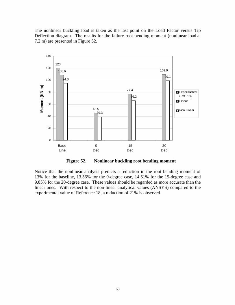
The nonlinear buckling load is taken as the last point on the Load Factor versus Tip Deflection diagram. The results for the failure root bending moment (nonlinear load at 7.2 m) are presented in Figure 52.
120
108.6
45.5
77.4
109.9
94.8
39.3
66.2
99.1
0
20
40
60
80
100
120
140
BaseLine
0Deg
15Deg
20Deg
Mom
ent (
KN
-m)
Experimental(Ref. 18)Linear
Non Linear
Figure 52. Nonlinear buckling root bending moment
Notice that the nonlinear analysis predicts a reduction in the root bending moment of 13% for the baseline, 13.56% for the 0-degree case, 14.51% for the 15-degree case and 9.85% for the 20-degree case. These values should be regarded as more accurate than the linear ones. With respect to the non-linear analytical values (ANSYS) compared to the experimental value of Reference 18, a reduction of 21% is observed.
64
RECOMMENDATIONS AND CONCLUSIONS The purpose of this study was to compare the baseline e-glass design of the Northern Power Systems NPS-100 prototype wind turbine rotor blade with twist-coupled, carbon-hybrid designs. Twist-coupled carbon designs were obtained by changing the unidirectional fibers in the spar caps to off-axis carbon fibers. The assumption was made that the carbon blades should deflect the same amount as the baseline for the unit load condition. In order to investigate these issues, four ANSYS finite element models were created using NuMAD. The deflection results show that similar flapwise deflections were obtained for all of the carbon-hybrid designs. The stiffer carbon fibers resulted in a reduction of the spar cap thickness: 43% of the baseline thickness for the 0-degree carbon, 63% for the 15-degree carbon, and 82% for the 20-degree carbon. These reductions in spar cap thickness also had an impact on the buckling loads. A decrease in the linear buckling load of 58% occurred for the 0-degree carbon design with 29% for the 15-degree carbon design. The 20-degree carbon design had approximately the same linear buckling load as the baseline design. This can be explained by the fact that the buckling load is proportional to the spar cap bending stiffness which depends on the cube of the thickness. It is interesting to notice that although the 20-degree carbon design is 82% of the original thickness, the buckling load remains close to the baseline buckling load. For a complex design the buckling is obviously dependent on other design details that require further investigation. The carbon-hybrid designs are all lower weight designs, which directly impacts the blade inertia loads. Reductions in weight for the 3 carbon designs are 19% for the 0-degree case, 14% for the 15-degree case and 9 % for the 20-degree case. Since all of these designs were limited to carbon substitution in the spar caps only, there is a substantial potential for further weight reduction. The twist-coupled designs produced a maximum twist of 1.2º for the 15-degree carbon design and 1.4º for the 20-degree carbon design. These results substantiate earlier studies on bend-twist coupled designs that indicated a good level of coupling for a fiber angle of 20º. Obviously the best design is one that provides enough coupling for fatigue loads alleviation and at the same time does not result in a substantial cost or weight increase or lowered aerodynamic performance. Further detailed studies are required to determine whether the current designs provide enough coupling. For both carbon designs the level of coupling was found to be maximum near the 50% span region. As previously mentioned, the present results are based on designs with off-axis carbon fibers only in the spar caps. The spar starts between blade stations 1 and 2. This means that the region of the blade with the maximum bending moment is not twisting. However, the blade is so stiff near the root that any twisting, regardless of coupling, is unlikely. Further studies are required to determine whether partial span coupling can be used to obtain the desired amount of twist. Another assumption that requires further validation is the maximum deflection limitation. The twist-coupled designs should have lower loads than the baseline design for the same extreme wind condition; thus, the deflection limitation might be too conservative. Dynamic loads analyses are required to determine the overall effect.
65
Two high strain areas were identified in the blade: the first between stations 800 and 2400, and the second one near station 8700. The maximum strains observed correspond to the leading edge, the shear web flange, and the rear and forward spar cap transitions where the material changes drastically in the circumferential direction. It is clear that these areas require some modifications of the structural details to minimize localized concentrations. It is imperative to investigate ways of transitioning in a smoother fashion. Several lay ups and material combinations need to be tested to evaluate the overall static strength as well as the fatigue characteristics. Our results indicate that although there is no single layer or group of layers that show a problematic strain trend, there is a tendency for the DBM1708/DBM1208 (+45/-45) glass layer to have high strain levels, which is not problematic as long as these layers have acceptable static and fatigue margins. The current results demonstrate that the levels of strain do not increase significantly when the off-axis fibers are introduced. This is an encouraging result, although it is important to remember that the carbon design allowable strains will likely be lower than the e-glass design allowable strains. If coupling were also introduced into the skins the nose strains would be even higher, which could be a reason to stay away from designs with full coupling in the skin. Finally, a few comments on NuMAD are in order. NuMAD demonstrated its great potential in helping the designer/analyst to create a model of a given blade with a great savings of time and effort. A set of basic initial geometric and structural data are required to begin the design/analysis process with NuMAD. Once the information is available the process of modeling is straightforward since NuMAD offers a user-friendly interface that translates the geometric and structural details of the blade into a set of instructions that the ANSYS finite element software can use to create the model. NuMAD is not 100% compatible with parametric studies where the basic design remains but some variables require modification; i.e., layer thickness, materials or fiber orientation. NuMAD must be used to manually modify these variables, and although this is not a difficult process by itself, it can become very tedious and prone to cause errors since the amount of information is considerable for detailed models. This problem can be overcome if the user is able to write macro files capable of reading and altering NuMAD’s output files in an automated fashion, but this is inconvenient in that the user must be familiar with ANSYS commands and structure and then generate the macro files that are required to modify these variables. If this feature could be built into NuMAD, then parametric studies would be greatly simplified and a broader spectrum of cases and configurations could be rapidly analyzed. At the time of writing we were aware that several efforts have already begun to add this automated capability. We look forward for these new versions of NuMAD. Overall, NuMAD is a valuable tool that greatly enhances the design/analysis process for a realistic wind turbine blade.
66
REFERENCES 1. D. Ancona, J. McVeigh, “Wind Turbine-Materials and Manufacturing Fact Sheet”
OIT-DOE Web site: http://www.oit.doe.gov/bestpractices/energymatters/emextra /pdfs/wind_materials.pdf
2. D.A. Spera, “Fatigue Design in Wind Turbines”, Wind Turbine Technology-Fundamental Concepts in Wind turbine Engineering, ASME Press,1998
3. N. M. Karaolis, P. J. Mussgrove, and G. Jeronimidis G, “Active and Passive Aeroelastic Power Control using Asymmetric Fibre Reinforced Laminates for Wind Turbine Blades,” Proc. 10th British Wind Energy Conf., D. J. Milbrow, Ed., London, March 22-24, 1988.
4. D. W. Lobitz, D. J. Laino, “Load Mitigation with Twist-Coupled HAWT Blades,” AIAA Paper 99-0033, 1999 ASME Wind Energy Symposium, Reno, NV, January 1999.
5. D. Lobitz, P. Veers, D. Laino, “Performance of Twist-Coupled Blades on Variable Speed Rotors,” AIAA 2000-0062, 2000 ASME Wind Energy Symposium, Reno, January 2000.
6. D.W. Lobitz, P.S. Veers, G.R. Eisler, D.J. Laino, P.G. Migliore, and G. Bir, “The Use of Twist-Coupled Blades to Enhance the Performance of Horizontal Axis Wind Turbines,” SAND2001-1003, Sandia National Laboratories, Albuquerque, NM, May 2001.
7. C.-H. Ong, S. W. Tsai, “Design, Manufacture, and Testing of a Bend-Twist D-Spar,” AIAA paper 99-0025, 1999 ASME Wind Energy Symposium, Reno, NV, January 1999.
8. C.H. Ong and S.W. Tsai, “Design, Manufacture and Testing of a Bend-Twist D-Spar,” SAND99-1324, Sandia National Laboratories, Albuquerque, NM, June 1999.
9. C.H. Ong, S. W. Tsai, “The Use of Carbon Fibers in Wind Turbine Blade Design: A SERI-8 Blade Example,” Sandia National Laboratories, Report SAND2000-0478, March 2000.
10. T.D. Ashwill, P.S Veers, J.E Locke, et al, “Concepts for Adaptive Wind Turbine Blades”, AIAA Paper 2002-0028, 2002 Wind Energy Symposium, Reno, NV, January 2002.
11. D.L. Laird, NuMAD User’s Manual, SAND2001-2375, Sandia National Laboratories, Albuquerque, NM, August 2001.
12. ANSYS Theory Reference Manual, ANSYS Inc. 13. C. Libove, “Stresses and Rate of Twist in Single-Cell Thin-Walled Beams with
Anisotropic Walls,” AIAA Journal, Vol. 26, No. 9, Sept. 1998, pp. 1107-1118. 14. R. M. Jones, Mechanics of Composite Materials, Hemisphere Publishing, 1975. 15. L.R McKittrick, D.S Cairns, J. Mandell., D.C. Combs., D.A Rabern and R.D Van
Luchene, “Analysis of a Composite Blade Design for the AOC 10/50 Wind Turbine using a Finite Element Model”, Sandia National Laboratories, Report SAND 2001-1441, May 2001.
16. IEC 61400-1, Ed. 2, Wind Turbine Generator Systems – Part 1: Safety Requirements, International Electrotechnical Commission (IEC), Geneva, Switzerland, 1998.

67
17. J. E. Locke, I. Contreras, “The Implementation of Braided Composite Materials in the Design of a Bend-Twist Coupled Blade,” SAND2002-2425, Sandia National Laboratories, Albuquerque, NM, August 2002.
18. TPI Composites, Inc., “Blade Manufacturing Improvements Development of the ERS-100 Blade,” Sandia National Laboratories Report SAND2001-1381, May 2001.
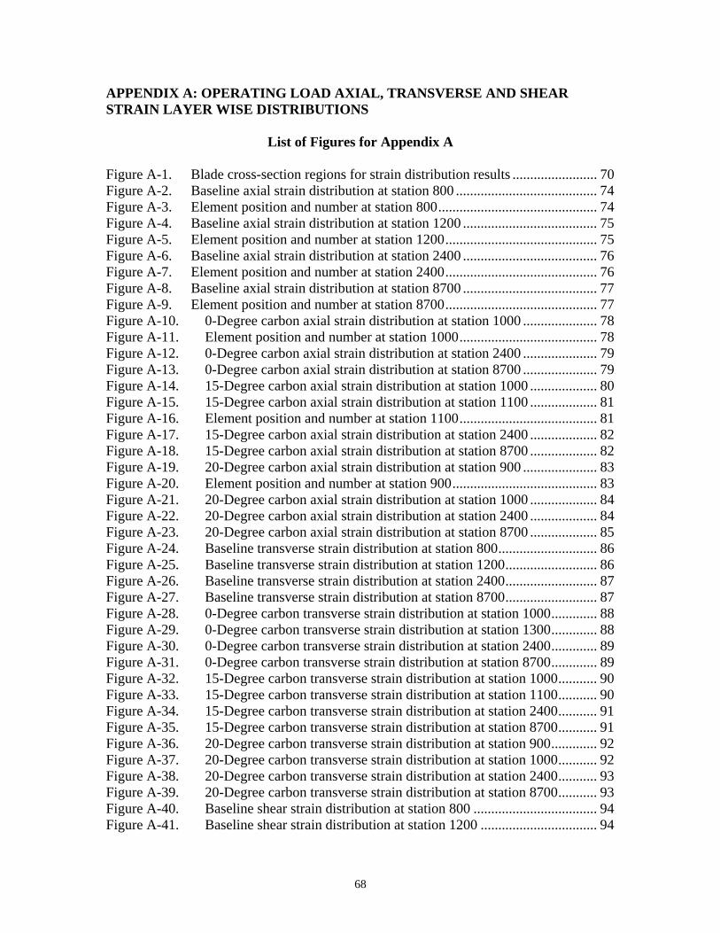
68
APPENDIX A: OPERATING LOAD AXIAL, TRANSVERSE AND SHEAR STRAIN LAYER WISE DISTRIBUTIONS
List of Figures for Appendix A Figure A-1. Blade cross-section regions for strain distribution results ........................ 70 Figure A-2. Baseline axial strain distribution at station 800 ........................................ 74 Figure A-3. Element position and number at station 800............................................. 74 Figure A-4. Baseline axial strain distribution at station 1200 ...................................... 75 Figure A-5. Element position and number at station 1200........................................... 75 Figure A-6. Baseline axial strain distribution at station 2400 ...................................... 76 Figure A-7. Element position and number at station 2400........................................... 76 Figure A-8. Baseline axial strain distribution at station 8700 ...................................... 77 Figure A-9. Element position and number at station 8700........................................... 77 Figure A-10. 0-Degree carbon axial strain distribution at station 1000 ..................... 78 Figure A-11. Element position and number at station 1000....................................... 78 Figure A-12. 0-Degree carbon axial strain distribution at station 2400 ..................... 79 Figure A-13. 0-Degree carbon axial strain distribution at station 8700 ..................... 79 Figure A-14. 15-Degree carbon axial strain distribution at station 1000 ................... 80 Figure A-15. 15-Degree carbon axial strain distribution at station 1100 ................... 81 Figure A-16. Element position and number at station 1100....................................... 81 Figure A-17. 15-Degree carbon axial strain distribution at station 2400 ................... 82 Figure A-18. 15-Degree carbon axial strain distribution at station 8700 ................... 82 Figure A-19. 20-Degree carbon axial strain distribution at station 900 ..................... 83 Figure A-20. Element position and number at station 900......................................... 83 Figure A-21. 20-Degree carbon axial strain distribution at station 1000 ................... 84 Figure A-22. 20-Degree carbon axial strain distribution at station 2400 ................... 84 Figure A-23. 20-Degree carbon axial strain distribution at station 8700 ................... 85 Figure A-24. Baseline transverse strain distribution at station 800............................ 86 Figure A-25. Baseline transverse strain distribution at station 1200.......................... 86 Figure A-26. Baseline transverse strain distribution at station 2400.......................... 87 Figure A-27. Baseline transverse strain distribution at station 8700.......................... 87 Figure A-28. 0-Degree carbon transverse strain distribution at station 1000............. 88 Figure A-29. 0-Degree carbon transverse strain distribution at station 1300............. 88 Figure A-30. 0-Degree carbon transverse strain distribution at station 2400............. 89 Figure A-31. 0-Degree carbon transverse strain distribution at station 8700............. 89 Figure A-32. 15-Degree carbon transverse strain distribution at station 1000........... 90 Figure A-33. 15-Degree carbon transverse strain distribution at station 1100........... 90 Figure A-34. 15-Degree carbon transverse strain distribution at station 2400........... 91 Figure A-35. 15-Degree carbon transverse strain distribution at station 8700........... 91 Figure A-36. 20-Degree carbon transverse strain distribution at station 900............. 92 Figure A-37. 20-Degree carbon transverse strain distribution at station 1000........... 92 Figure A-38. 20-Degree carbon transverse strain distribution at station 2400........... 93 Figure A-39. 20-Degree carbon transverse strain distribution at station 8700........... 93 Figure A-40. Baseline shear strain distribution at station 800 ................................... 94 Figure A-41. Baseline shear strain distribution at station 1200 ................................. 94
69
Figure A-42. Baseline shear strain distribution at station 2400 ................................. 95 Figure A-43. Baseline shear strain distribution at station 8700 ................................. 95 Figure A-44. 0-Degree carbon shear strain distribution at station 1000 .................... 96 Figure A-45. 0-Degree carbon shear strain distribution at station 1300 .................... 96 Figure A-46. 0-Degree carbon shear strain distribution at station 2400 .................... 97 Figure A-47. 0-Degree carbon shear strain distribution at station 8700 .................... 97 Figure A-48. 15-Degree carbon shear strain distribution at station 1000 .................. 98 Figure A-49. 15-Degree carbon shear strain distribution at station 1100 .................. 98 Figure A-50. 15-Degree carbon shear strain distribution at station 2400 .................. 99 Figure A-51. 15-Degree carbon shear strain distribution at station 8700 .................. 99 Figure A-52. 20-Degree carbon shear strain distribution at station 900 .................. 100 Figure A-53. 20-Degree carbon shear strain distribution at station 1000 ................ 100 Figure A-54. 20-Degree carbon shear strain distribution at station 2400 ................ 101 Figure A-55. 20-Degree carbon shear strain distribution at station 8700 ................ 101

70
Strain Distribution Results Strain distributions are shown for each of the following regions: I. Nose Region II. Forward Spar Cap III. Shear Web Flange IV. Aft Spar Cap V. Trailing Edge
Figure A-1. Blade cross-section regions for strain distribution results
I
II
III IVV
V
IV
IIIII
I
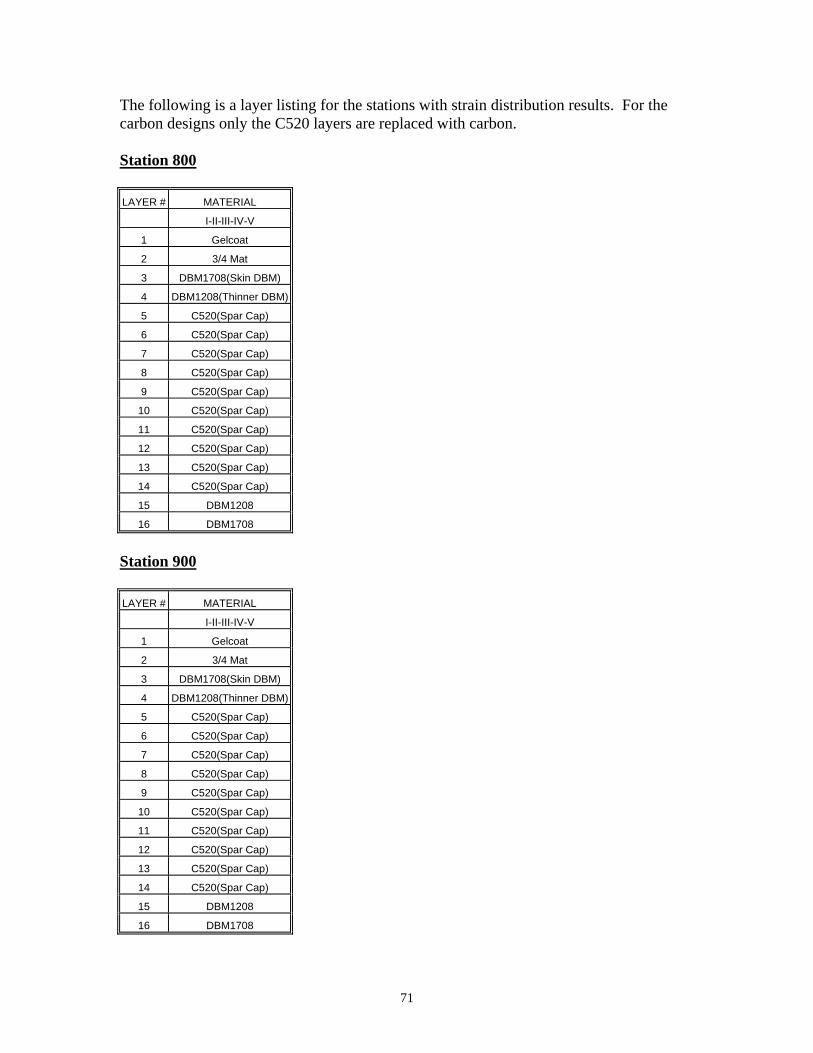
71
The following is a layer listing for the stations with strain distribution results. For the carbon designs only the C520 layers are replaced with carbon. Station 800 LAYER # MATERIAL
I-II-III-IV-V
1 Gelcoat
2 3/4 Mat
3 DBM1708(Skin DBM)
4 DBM1208(Thinner DBM)
5 C520(Spar Cap)
6 C520(Spar Cap)
7 C520(Spar Cap)
8 C520(Spar Cap)
9 C520(Spar Cap)
10 C520(Spar Cap)
11 C520(Spar Cap)
12 C520(Spar Cap)
13 C520(Spar Cap)
14 C520(Spar Cap)
15 DBM1208
16 DBM1708
Station 900 LAYER # MATERIAL
I-II-III-IV-V
1 Gelcoat
2 3/4 Mat
3 DBM1708(Skin DBM)
4 DBM1208(Thinner DBM)
5 C520(Spar Cap)
6 C520(Spar Cap)
7 C520(Spar Cap)
8 C520(Spar Cap)
9 C520(Spar Cap)
10 C520(Spar Cap)
11 C520(Spar Cap)
12 C520(Spar Cap)
13 C520(Spar Cap)
14 C520(Spar Cap)
15 DBM1208
16 DBM1708
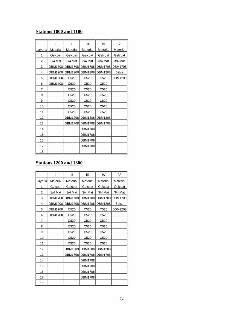
72
Stations 1000 and 1100
I II III IV V
Layer # Material Material Material Material Material
1 Gelcoat Gelcoat Gelcoat Gelcoat Gelcoat
2 3/4 Mat 3/4 Mat 3/4 Mat 3/4 Mat 3/4 Mat
3 DBM1708 DBM1708 DBM1708 DBM1708 DBM1708
4 DBM1208 DBM1208 DBM1208 DBM1208 Balsa
5 DBM1208 C520 C520 C520 DBM1208
6 DBM1708 C520 C520 C520
7 C520 C520 C520
8 C520 C520 C520
9 C520 C520 C520
10 C520 C520 C520
11 C520 C520 C520
12 DBM1208 DBM1208 DBM1208
13 DBM1708 DBM1708 DBM1708
14 DBM1708
15 DBM1708
16 DBM1708
17 DBM1708
18
Stations 1200 and 1300
I II III IV V Layer # Material Material Material Material Material
1 Gelcoat Gelcoat Gelcoat Gelcoat Gelcoat
2 3/4 Mat 3/4 Mat 3/4 Mat 3/4 Mat 3/4 Mat
3 DBM1708 DBM1708 DBM1708 DBM1708 DBM1708
4 DBM1208 DBM1208 DBM1208 DBM1208 Balsa
5 DBM1208 C520 C520 C520 DBM1208
6 DBM1708 C520 C520 C520
7 C520 C520 C520
8 C520 C520 C520
9 C520 C520 C520
10 C520 C520 C520
11 C520 C520 C520
12 DBM1208 DBM1208 DBM1208
13 DBM1708 DBM1708 DBM1708
14 DBM1708
15 DBM1708
16 DBM1708
17 DBM1708
18
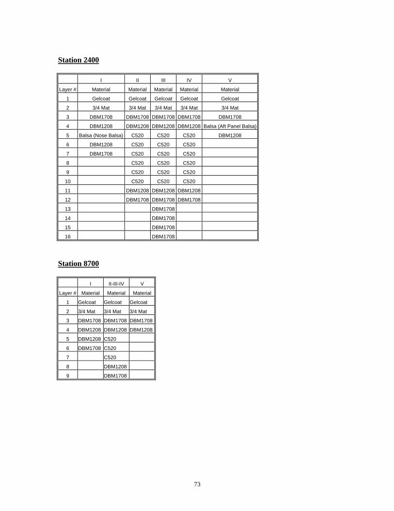
73
Station 2400
I II III IV V
Layer # Material Material Material Material Material
1 Gelcoat Gelcoat Gelcoat Gelcoat Gelcoat
2 3/4 Mat 3/4 Mat 3/4 Mat 3/4 Mat 3/4 Mat
3 DBM1708 DBM1708 DBM1708 DBM1708 DBM1708
4 DBM1208 DBM1208 DBM1208 DBM1208 Balsa (Aft Panel Balsa)
5 Balsa (Nose Balsa) C520 C520 C520 DBM1208
6 DBM1208 C520 C520 C520
7 DBM1708 C520 C520 C520
8 C520 C520 C520
9 C520 C520 C520
10 C520 C520 C520
11 DBM1208 DBM1208 DBM1208
12 DBM1708 DBM1708 DBM1708
13 DBM1708
14 DBM1708
15 DBM1708
16 DBM1708
Station 8700
I II-III-IV V
Layer # Material Material Material
1 Gelcoat Gelcoat Gelcoat
2 3/4 Mat 3/4 Mat 3/4 Mat
3 DBM1708 DBM1708 DBM1708
4 DBM1208 DBM1208 DBM1208
5 DBM1208 C520
6 DBM1708 C520
7 C520
8 DBM1208
9 DBM1708
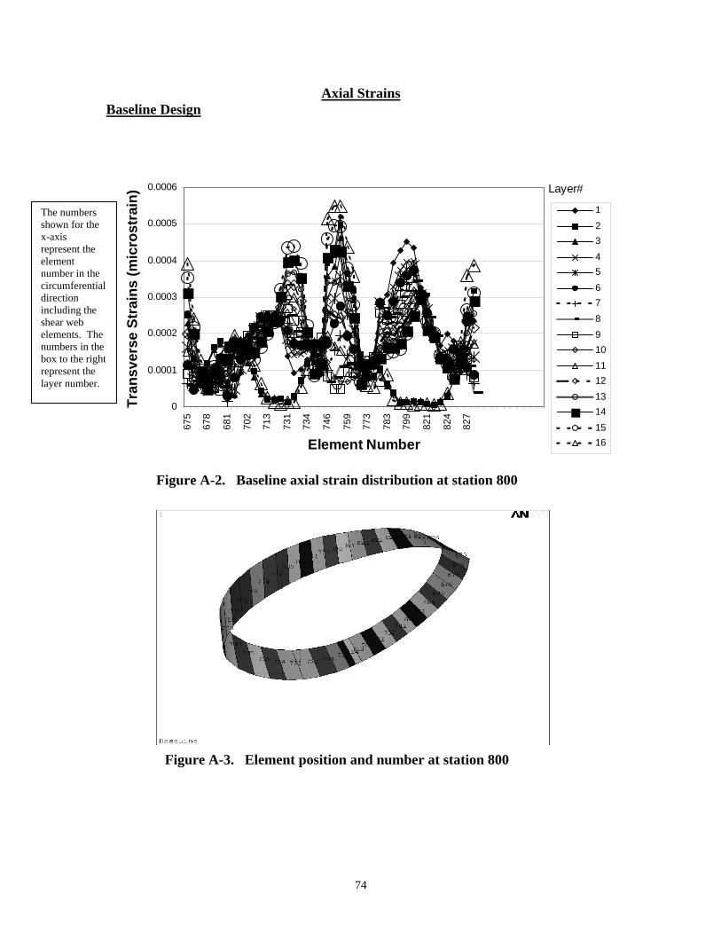
74
Axial Strains Baseline Design
0
0.0001
0.0002
0.0003
0.0004
0.0005
0.000667
5
678
681
702
713
731
734
746
759
773
783
799
821
824
827
Element Number
Tran
sver
se S
trai
ns (m
icro
stra
in)
12345678910111213141516
Layer#
Figure A-2. Baseline axial strain distribution at station 800
Figure A-3. Element position and number at station 800
The numbers shown for the x-axis represent the element number in the circumferential direction including the shear web elements. The numbers in the box to the right represent the layer number.
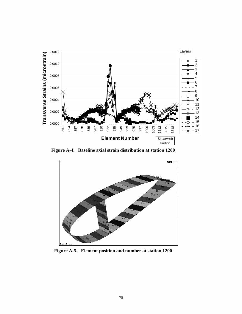
75
0.0000
0.0002
0.0004
0.0006
0.0008
0.0010
0.0012
851
854
857
878
889
907
910
922
935
949
959
975
997
1000
1003
3312
3315
3318
Element Number
Tran
sver
se S
trai
ns (m
icro
stra
in)
1234567891011121314151617
Layer#
Shearw eb Portion
Figure A-4. Baseline axial strain distribution at station 1200
Figure A-5. Element position and number at station 1200
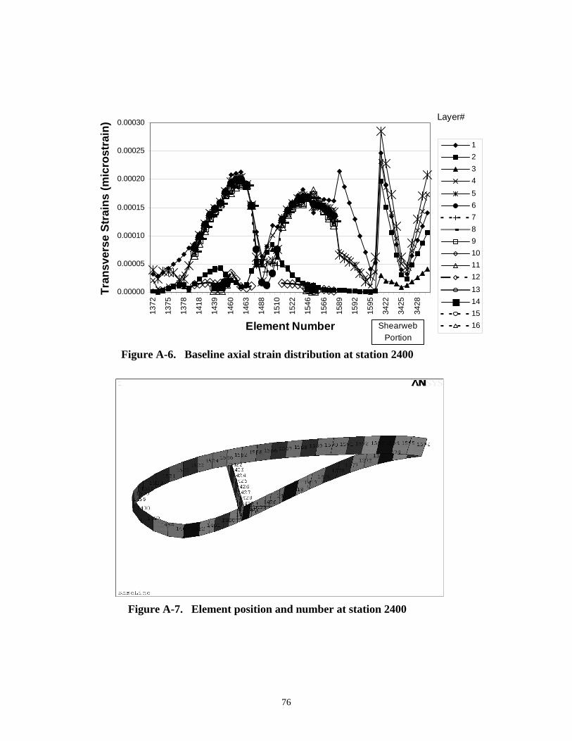
76
0.00000
0.00005
0.00010
0.00015
0.00020
0.00025
0.00030
1372
1375
1378
1418
1439
1460
1463
1488
1510
1522
1546
1566
1589
1592
1595
3422
3425
3428
Element Number
Tran
sver
se S
trai
ns (m
icro
stra
in)
12345678910111213141516
Layer#
Shearweb Portion
Figure A-6. Baseline axial strain distribution at station 2400
Figure A-7. Element position and number at station 2400
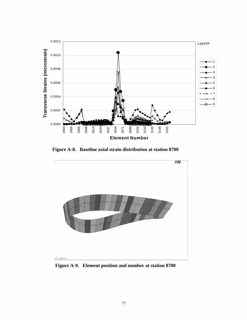
77
0.0000
0.0002
0.0004
0.0006
0.0008
0.0010
0.0012
2963
2966
2969
2998
3013
3034
3037
3054
3071
3086
3101
3120
3145
3148
3151
Element Number
Tran
sver
se S
trai
ns (m
icro
stra
in)
1
2
3
4
5
6
7
8
9
Layer#
Figure A-8. Baseline axial strain distribution at station 8700
Figure A-9. Element position and number at station 8700
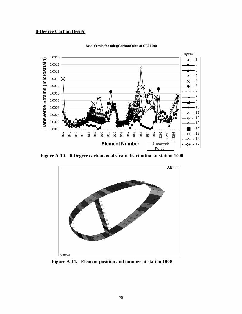
78
0-Degree Carbon Design
Axial Strain for 0degCarbonSubs at STA1000
0.0000
0.0002
0.0004
0.0006
0.0008
0.0010
0.0012
0.0014
0.0016
0.0018
0.0020
837
840
843
870
885
897
900
918
933
939
957
969
981
984
987
3292
3295
3298
Element Number
Tran
sver
se S
trai
ns (m
icro
stra
in) 1
234567891011121314151617
Layer#
Shearweb Portion
Figure A-10. 0-Degree carbon axial strain distribution at station 1000
Figure A-11. Element position and number at station 1000
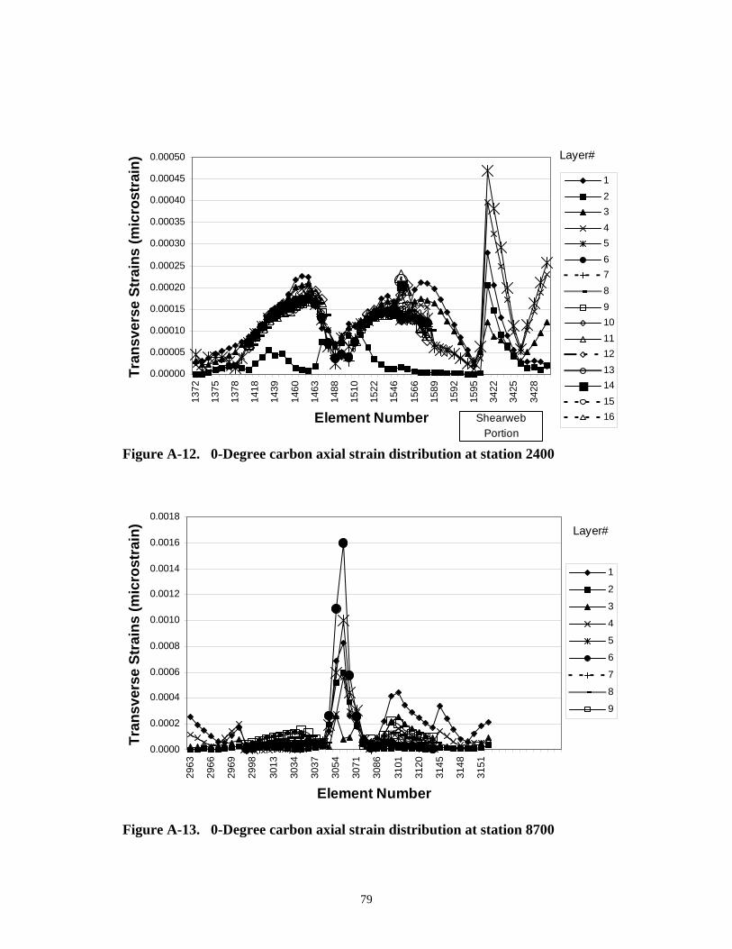
79
0.00000
0.00005
0.00010
0.00015
0.00020
0.00025
0.00030
0.00035
0.00040
0.00045
0.00050
1372
1375
1378
1418
1439
1460
1463
1488
1510
1522
1546
1566
1589
1592
1595
3422
3425
3428
Element Number
Tran
sver
se S
trai
ns (m
icro
stra
in)
12345678910111213141516
Layer#
Shearweb Portion
Figure A-12. 0-Degree carbon axial strain distribution at station 2400
0.0000
0.0002
0.0004
0.0006
0.0008
0.0010
0.0012
0.0014
0.0016
0.0018
2963
2966
2969
2998
3013
3034
3037
3054
3071
3086
3101
3120
3145
3148
3151
Element Number
Tran
sver
se S
trai
ns (m
icro
stra
in)
1
2
3
4
5
6
7
8
9
Layer#
Figure A-13. 0-Degree carbon axial strain distribution at station 8700
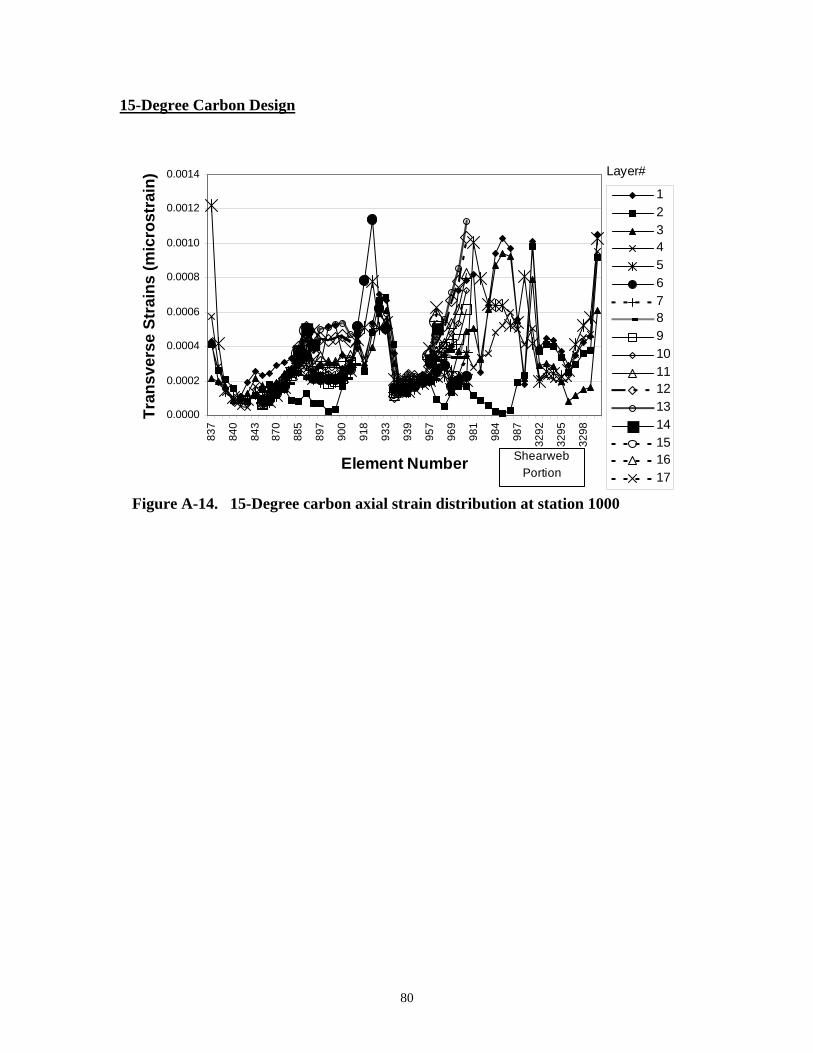
80
15-Degree Carbon Design
0.0000
0.0002
0.0004
0.0006
0.0008
0.0010
0.0012
0.0014
837
840
843
870
885
897
900
918
933
939
957
969
981
984
987
3292
3295
3298
Element Number
Tran
sver
se S
trai
ns (m
icro
stra
in)
1234567891011121314151617
Layer#
Shearweb Portion
Figure A-14. 15-Degree carbon axial strain distribution at station 1000
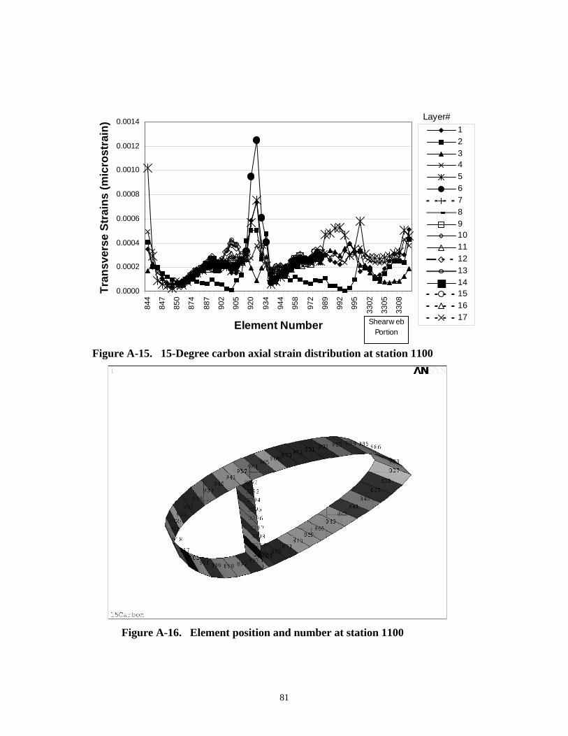
81
0.0000
0.0002
0.0004
0.0006
0.0008
0.0010
0.0012
0.0014
844
847
850
874
887
902
905
920
934
944
958
972
989
992
995
3302
3305
3308
Element Number
Tran
sver
se S
trai
ns (m
icro
stra
in)
1234567891011121314151617
Layer#
Shearw eb Portion
Figure A-15. 15-Degree carbon axial strain distribution at station 1100
Figure A-16. Element position and number at station 1100
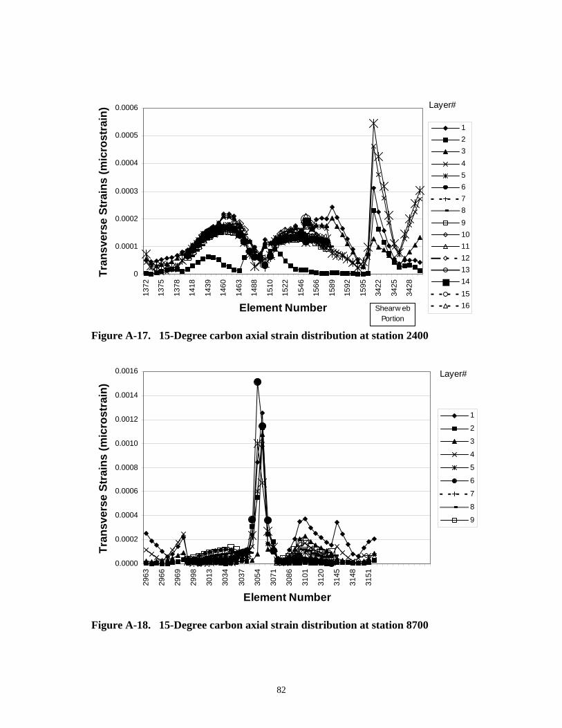
82
0
0.0001
0.0002
0.0003
0.0004
0.0005
0.0006
1372
1375
1378
1418
1439
1460
1463
1488
1510
1522
1546
1566
1589
1592
1595
3422
3425
3428
Element Number
Tran
sver
se S
trai
ns (m
icro
stra
in)
12345678910111213141516
Layer#
Shearw eb Portion
Figure A-17. 15-Degree carbon axial strain distribution at station 2400
0.0000
0.0002
0.0004
0.0006
0.0008
0.0010
0.0012
0.0014
0.0016
2963
2966
2969
2998
3013
3034
3037
3054
3071
3086
3101
3120
3145
3148
3151
Element Number
Tran
sver
se S
trai
ns (m
icro
stra
in)
1
2
3
4
5
6
7
8
9
Layer#
Figure A-18. 15-Degree carbon axial strain distribution at station 8700
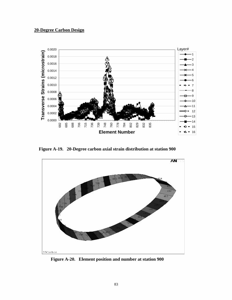
83
20-Degree Carbon Design
0.0000
0.0002
0.0004
0.0006
0.0008
0.0010
0.0012
0.0014
0.0016
0.0018
0.0020
682
685
688
706
715
736
739
748
760
778
784
802
829
832
835
Element Number
Tran
sver
se S
trai
ns (m
icro
stra
in)
1
2
3
4
5
6
7
8
9
10
11
12
13
14
15
16
Layer#
Figure A-19. 20-Degree carbon axial strain distribution at station 900
Figure A-20. Element position and number at station 900
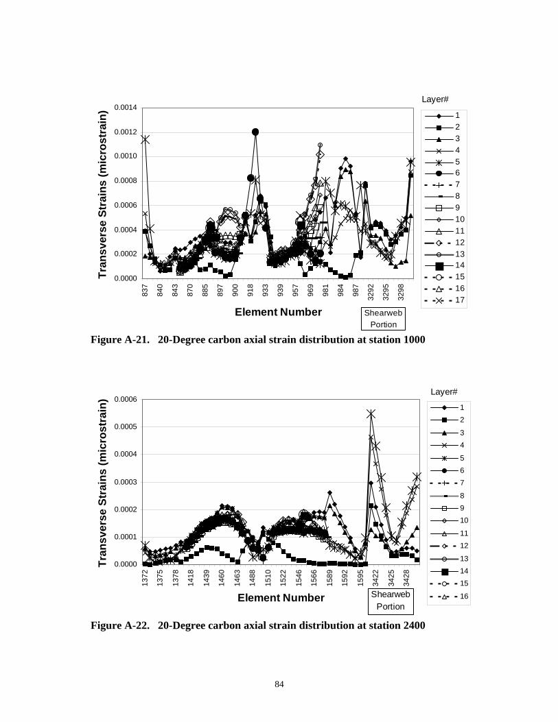
84
0.0000
0.0002
0.0004
0.0006
0.0008
0.0010
0.0012
0.0014
837
840
843
870
885
897
900
918
933
939
957
969
981
984
987
3292
3295
3298
Element Number
Tran
sver
se S
trai
ns (m
icro
stra
in) 1
234567891011121314151617
Layer#
Shearweb Portion
Figure A-21. 20-Degree carbon axial strain distribution at station 1000
0.0000
0.0001
0.0002
0.0003
0.0004
0.0005
0.0006
1372
1375
1378
1418
1439
1460
1463
1488
1510
1522
1546
1566
1589
1592
1595
3422
3425
3428
Element Number
Tran
sver
se S
trai
ns (m
icro
stra
in)
12
34
567
8910
1112
131415
16
Layer#
Shearweb Portion
Figure A-22. 20-Degree carbon axial strain distribution at station 2400
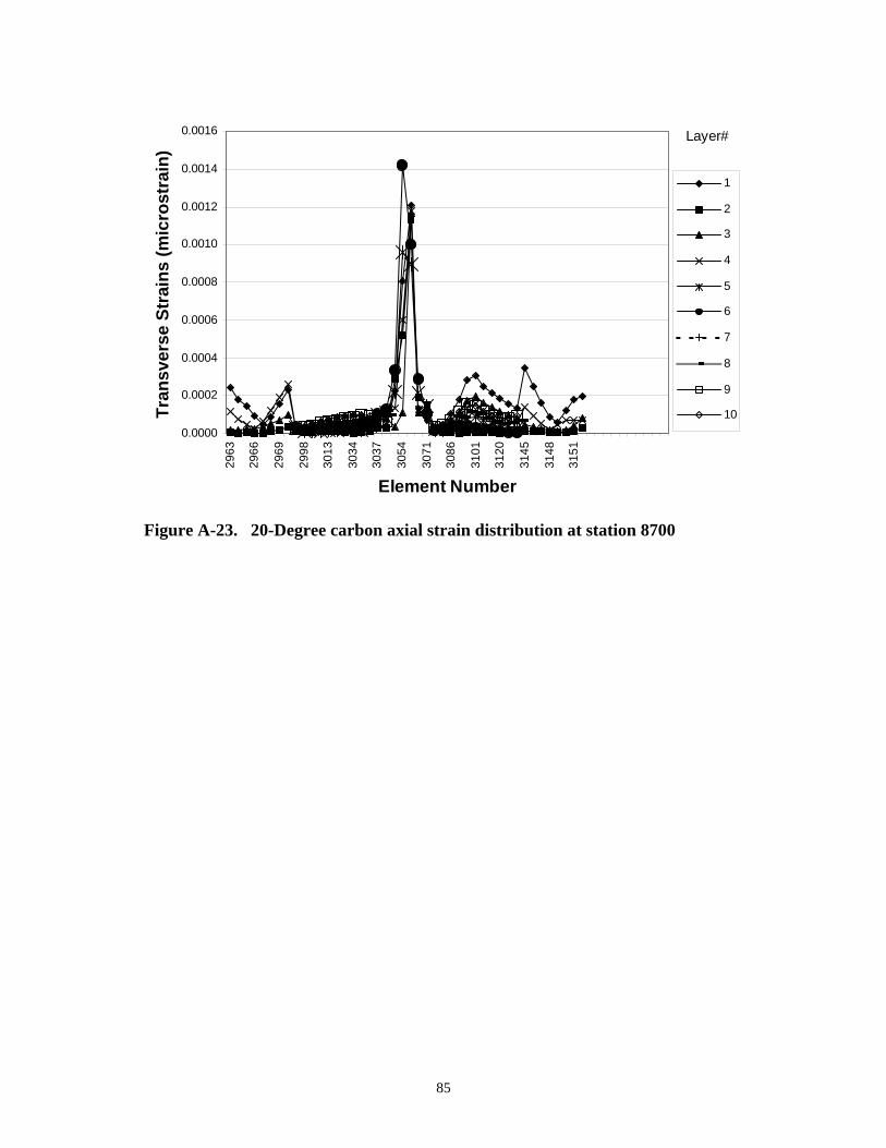
85
0.0000
0.0002
0.0004
0.0006
0.0008
0.0010
0.0012
0.0014
0.0016
2963
2966
2969
2998
3013
3034
3037
3054
3071
3086
3101
3120
3145
3148
3151
Element Number
Tran
sver
se S
trai
ns (m
icro
stra
in)
1
2
3
4
5
6
7
8
9
10
Layer#
Figure A-23. 20-Degree carbon axial strain distribution at station 8700
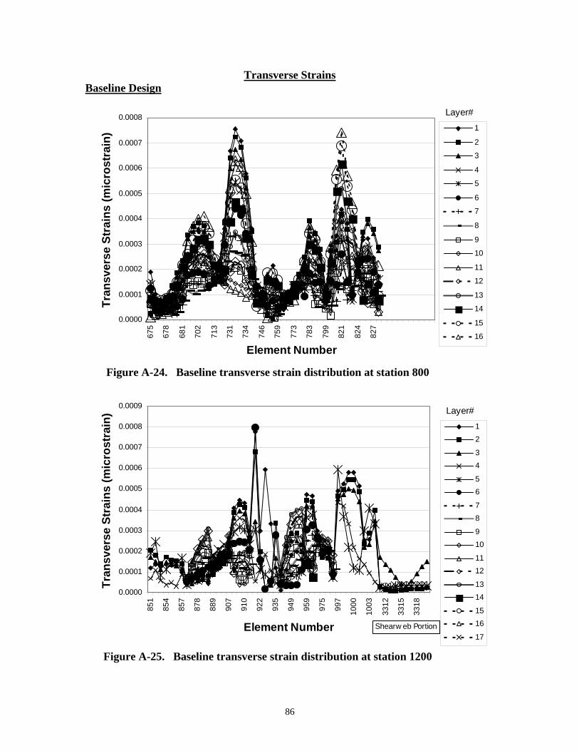
86
Transverse Strains Baseline Design
0.0000
0.0001
0.0002
0.0003
0.0004
0.0005
0.0006
0.0007
0.0008
675
678
681
702
713
731
734
746
759
773
783
799
821
824
827
Element Number
Tran
sver
se S
trai
ns (m
icro
stra
in) 1
2
3
4
5
6
7
8
9
10
11
12
13
14
15
16
Layer#
Figure A-24. Baseline transverse strain distribution at station 800
0.0000
0.0001
0.0002
0.0003
0.0004
0.0005
0.0006
0.0007
0.0008
0.0009
851
854
857
878
889
907
910
922
935
949
959
975
997
1000
1003
3312
3315
3318
Element Number
Tran
sver
se S
trai
ns (m
icro
stra
in)
12
34
56
78
910
1112
1314
1516
17
Layer#
Shearw eb Portion
Figure A-25. Baseline transverse strain distribution at station 1200
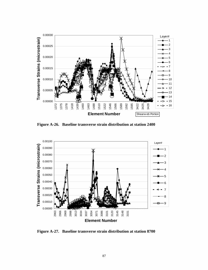
87
0.00000
0.00005
0.00010
0.00015
0.00020
0.00025
0.00030
1372
1375
1378
1418
1439
1460
1463
1488
1510
1522
1546
1566
1589
1592
1595
3422
3425
3428
Element Number
Tran
sver
se S
trai
ns (m
icro
stra
in)
12345678910111213141516
Layer#
Shearw eb Portion
Figure A-26. Baseline transverse strain distribution at station 2400
0.00000
0.00010
0.00020
0.00030
0.00040
0.00050
0.00060
0.00070
0.00080
0.00090
0.00100
2963
2966
2969
2998
3013
3034
3037
3054
3071
3086
3101
3120
3145
3148
3151
Element Number
Tran
sver
se S
trai
ns (m
icro
stra
in)
1
2
3
4
5
6
7
8
9
Layer#
Figure A-27. Baseline transverse strain distribution at station 8700
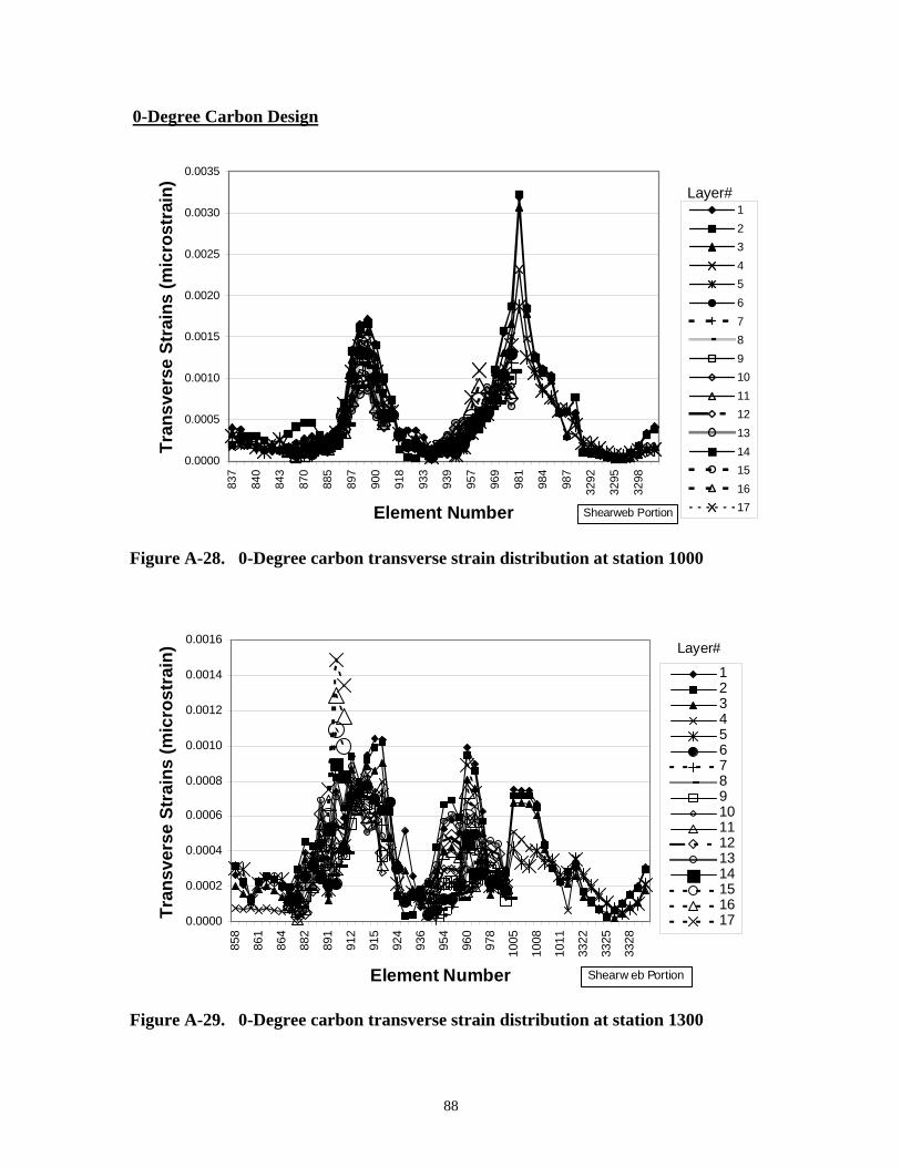
88
0-Degree Carbon Design
0.0000
0.0005
0.0010
0.0015
0.0020
0.0025
0.0030
0.0035
837
840
843
870
885
897
900
918
933
939
957
969
981
984
987
3292
3295
3298
Element Number
Tran
sver
se S
trai
ns (m
icro
stra
in)
1234567891011121314151617
Layer#
Shearweb Portion
Figure A-28. 0-Degree carbon transverse strain distribution at station 1000
0.0000
0.0002
0.0004
0.0006
0.0008
0.0010
0.0012
0.0014
0.0016
858
861
864
882
891
912
915
924
936
954
960
978
1005
1008
1011
3322
3325
3328
Element Number
Tran
sver
se S
trai
ns (m
icro
stra
in)
1234567891011121314151617
Layer#
Shearw eb Portion
Figure A-29. 0-Degree carbon transverse strain distribution at station 1300
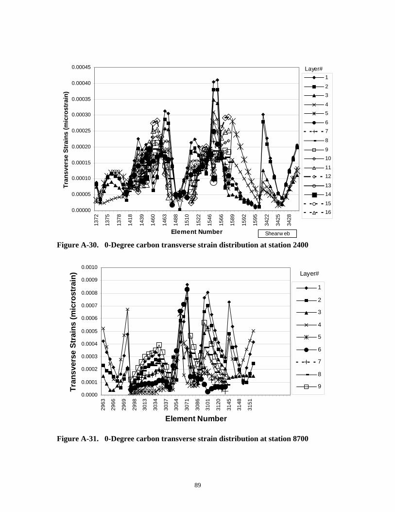
89
0.00000
0.00005
0.00010
0.00015
0.00020
0.00025
0.00030
0.00035
0.00040
0.00045
1372
1375
1378
1418
1439
1460
1463
1488
1510
1522
1546
1566
1589
1592
1595
3422
3425
3428
Element Number
Tran
sver
se S
trai
ns (m
icro
stra
in)
1
23
45
67
8
910
1112
1314
1516
Layer#
Shearw eb Figure A-30. 0-Degree carbon transverse strain distribution at station 2400
0.0000
0.0001
0.0002
0.0003
0.0004
0.0005
0.0006
0.0007
0.0008
0.0009
0.0010
2963
2966
2969
2998
3013
3034
3037
3054
3071
3086
3101
3120
3145
3148
3151
Element Number
Tran
sver
se S
trai
ns (m
icro
stra
in)
1
2
3
4
5
6
7
8
9
Layer#
Figure A-31. 0-Degree carbon transverse strain distribution at station 8700
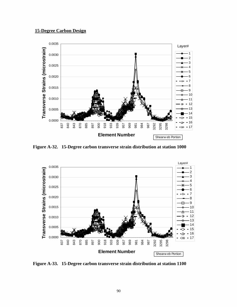
90
15-Degree Carbon Design
0.0000
0.0005
0.0010
0.0015
0.0020
0.0025
0.0030
0.0035
837
840
843
870
885
897
900
918
933
939
957
969
981
984
987
3292
3295
3298
Element Number
Tran
sver
se S
trai
ns (m
icro
stra
in)
1234567891011121314151617
Layer#
Shearw eb Portion
Figure A-32. 15-Degree carbon transverse strain distribution at station 1000
0.0000
0.0005
0.0010
0.0015
0.0020
0.0025
0.0030
0.0035
837
840
843
870
885
897
900
918
933
939
957
969
981
984
987
3292
3295
3298
Element Number
Tran
sver
se S
trai
ns (m
icro
stra
in) 1
234567891011121314151617
Layer#
Shearw eb Portion
Figure A-33. 15-Degree carbon transverse strain distribution at station 1100
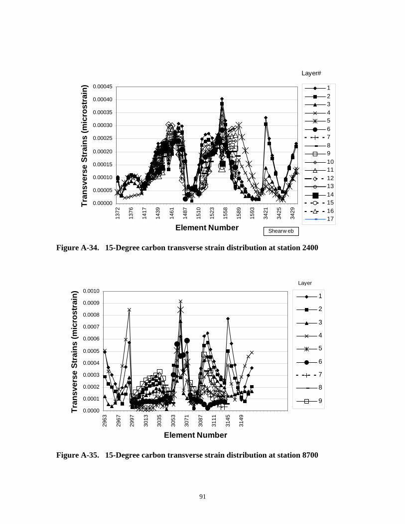
91
0.00000
0.00005
0.00010
0.00015
0.00020
0.00025
0.00030
0.00035
0.00040
0.00045
1372
1376
1417
1439
1461
1487
1510
1523
1558
1589
1593
3421
3425
3429
Element Number
Tran
sver
se S
trai
ns (m
icro
stra
in) 1
234567891011121314151617
Layer#
Shearw eb
Figure A-34. 15-Degree carbon transverse strain distribution at station 2400
0.0000
0.0001
0.0002
0.0003
0.0004
0.0005
0.0006
0.0007
0.0008
0.0009
0.0010
2963
2967
2997
3013
3035
3053
3071
3087
3111
3145
3149
Element Number
Tran
sver
se S
trai
ns (m
icro
stra
in)
1
2
3
4
5
6
7
8
9
Layer
Figure A-35. 15-Degree carbon transverse strain distribution at station 8700
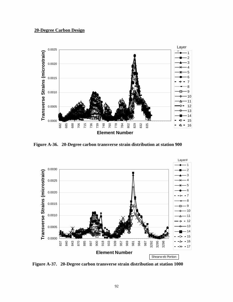
92
20-Degree Carbon Design
0.0000
0.0005
0.0010
0.0015
0.0020
0.0025
682
685
688
706
715
736
739
748
760
778
784
802
829
832
835
Element Number
Tran
sver
se S
trai
ns (m
icro
stra
in) 1
2345678910111213141516
Layer#
Figure A-36. 20-Degree carbon transverse strain distribution at station 900
0.0000
0.0005
0.0010
0.0015
0.0020
0.0025
0.0030
837
840
843
870
885
897
900
918
933
939
957
969
981
984
987
3292
3295
3298
Element Number
Tran
sver
se S
trai
ns (m
icro
stra
in)
1234567891011121314151617
Layer#
Shearw eb Portion
Figure A-37. 20-Degree carbon transverse strain distribution at station 1000
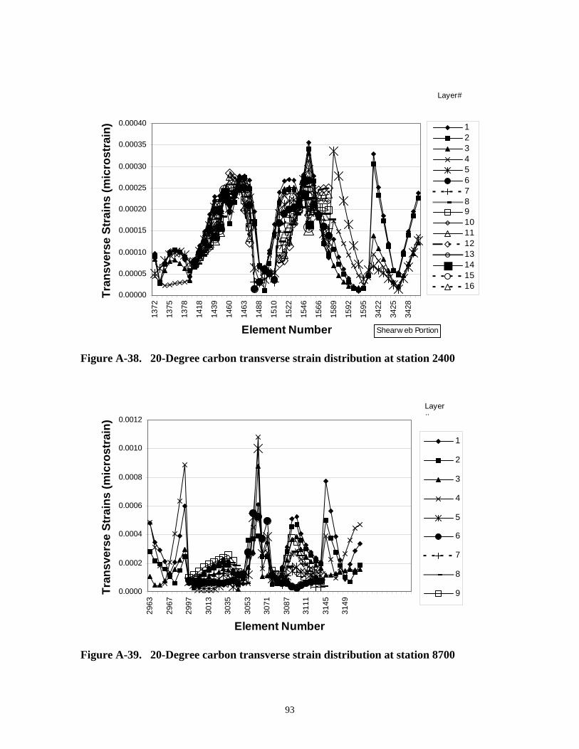
93
0.00000
0.00005
0.00010
0.00015
0.00020
0.00025
0.00030
0.00035
0.00040
1372
1375
1378
1418
1439
1460
1463
1488
1510
1522
1546
1566
1589
1592
1595
3422
3425
3428
Element Number
Tran
sver
se S
trai
ns (m
icro
stra
in) 1
2345678910111213141516
Layer#
Shearw eb Portion
Figure A-38. 20-Degree carbon transverse strain distribution at station 2400
0.0000
0.0002
0.0004
0.0006
0.0008
0.0010
0.0012
2963
2967
2997
3013
3035
3053
3071
3087
3111
3145
3149
Element Number
Tran
sver
se S
trai
ns (m
icro
stra
in)
1
2
3
4
5
6
7
8
9
Layer#
Figure A-39. 20-Degree carbon transverse strain distribution at station 8700
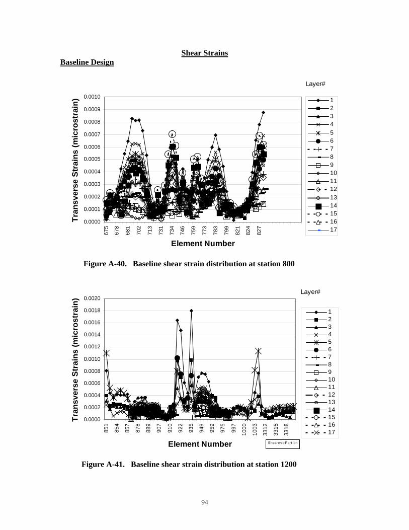
94
Shear Strains Baseline Design
0.0000
0.0001
0.0002
0.0003
0.0004
0.0005
0.0006
0.0007
0.0008
0.0009
0.0010
675
678
681
702
713
731
734
746
759
773
783
799
821
824
827
Element Number
Tran
sver
se S
trai
ns (m
icro
stra
in) 1
234567891011121314151617
Layer#
Figure A-40. Baseline shear strain distribution at station 800
0.0000
0.0002
0.0004
0.0006
0.0008
0.0010
0.0012
0.0014
0.0016
0.0018
0.0020
851
854
857
878
889
907
910
922
935
949
959
975
997
1000
1003
3312
3315
3318
Element Number
Tran
sver
se S
trai
ns (m
icro
stra
in)
1234567891011121314151617
Layer#
Shearweb Port ion
Figure A-41. Baseline shear strain distribution at station 1200
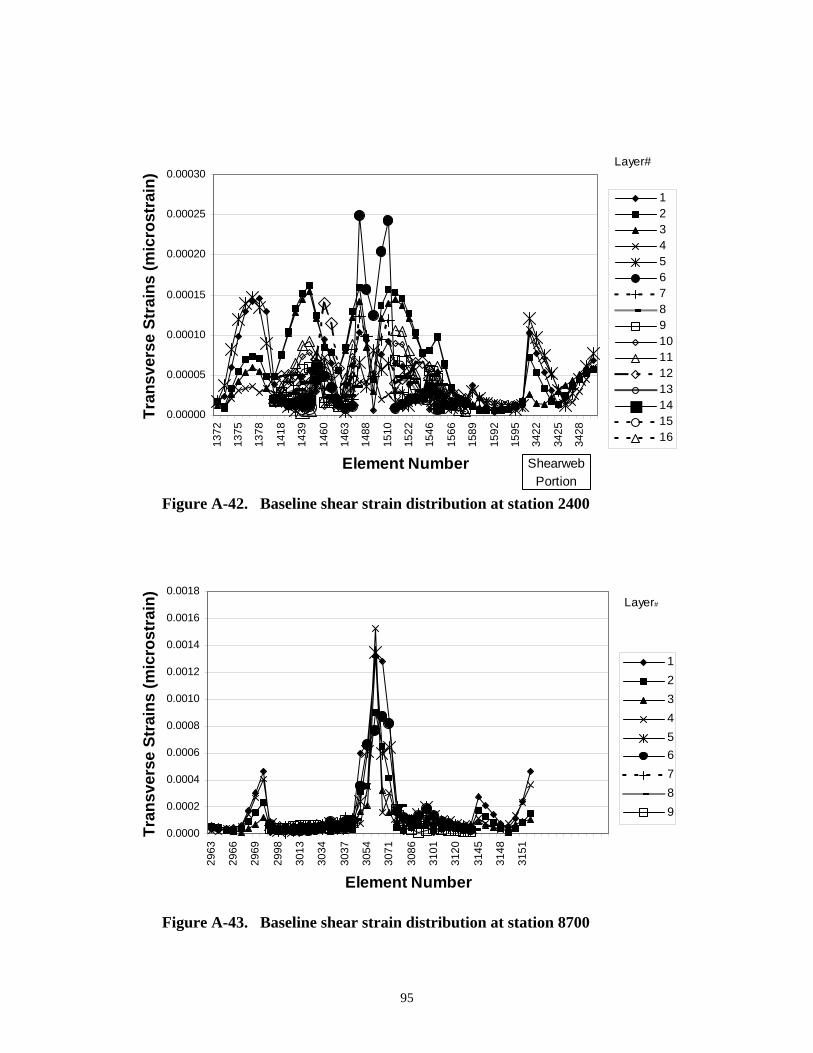
95
0.00000
0.00005
0.00010
0.00015
0.00020
0.00025
0.00030
1372
1375
1378
1418
1439
1460
1463
1488
1510
1522
1546
1566
1589
1592
1595
3422
3425
3428
Element Number
Tran
sver
se S
trai
ns (m
icro
stra
in)
12345678910111213141516
Layer#
Shearweb Portion
Figure A-42. Baseline shear strain distribution at station 2400
0.0000
0.0002
0.0004
0.0006
0.0008
0.0010
0.0012
0.0014
0.0016
0.0018
2963
2966
2969
2998
3013
3034
3037
3054
3071
3086
3101
3120
3145
3148
3151
Element Number
Tran
sver
se S
trai
ns (m
icro
stra
in)
123456789
Layer#
Figure A-43. Baseline shear strain distribution at station 8700
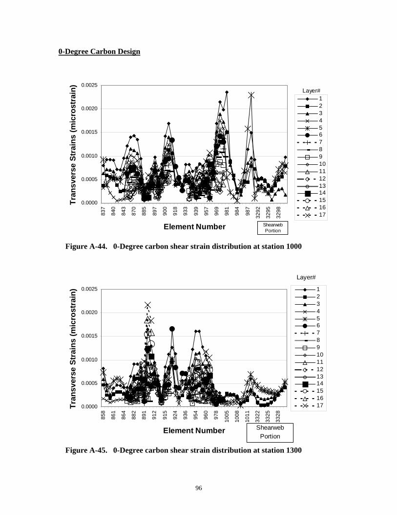
96
0-Degree Carbon Design
0.0000
0.0005
0.0010
0.0015
0.0020
0.0025
837
840
843
870
885
897
900
918
933
939
957
969
981
984
987
3292
3295
3298
Element Number
Tran
sver
se S
trai
ns (m
icro
stra
in)
1234567891011121314151617
Layer#
Shearweb Portion
Figure A-44. 0-Degree carbon shear strain distribution at station 1000
0.0000
0.0005
0.0010
0.0015
0.0020
0.0025
858
861
864
882
891
912
915
924
936
954
960
978
1005
1008
1011
3322
3325
3328
Element Number
Tran
sver
se S
trai
ns (m
icro
stra
in) 1
234567891011121314151617
Layer#
Shearweb Portion
Figure A-45. 0-Degree carbon shear strain distribution at station 1300
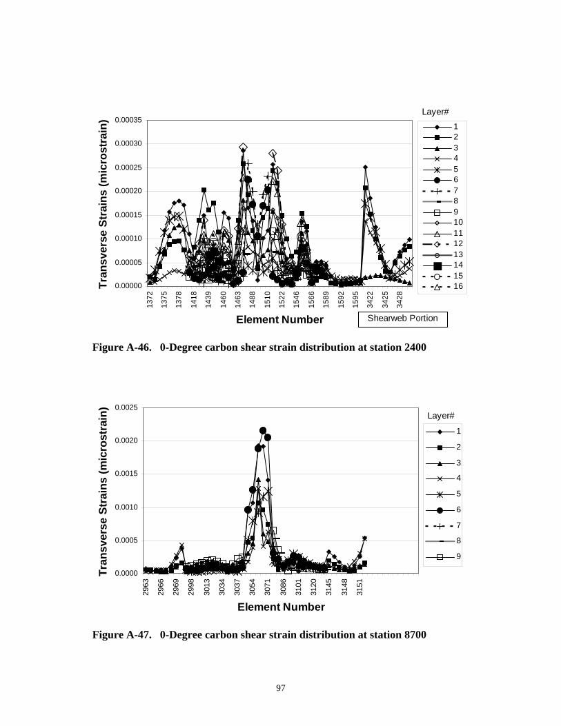
97
0.00000
0.00005
0.00010
0.00015
0.00020
0.00025
0.00030
0.00035
1372
1375
1378
1418
1439
1460
1463
1488
1510
1522
1546
1566
1589
1592
1595
3422
3425
3428
Element Number
Tran
sver
se S
trai
ns (m
icro
stra
in)
12345678910111213141516
Layer#
Shearweb Portion
Figure A-46. 0-Degree carbon shear strain distribution at station 2400
0.0000
0.0005
0.0010
0.0015
0.0020
0.0025
2963
2966
2969
2998
3013
3034
3037
3054
3071
3086
3101
3120
3145
3148
3151
Element Number
Tran
sver
se S
trai
ns (m
icro
stra
in)
1
2
3
4
5
6
7
8
9
Layer#
Figure A-47. 0-Degree carbon shear strain distribution at station 8700
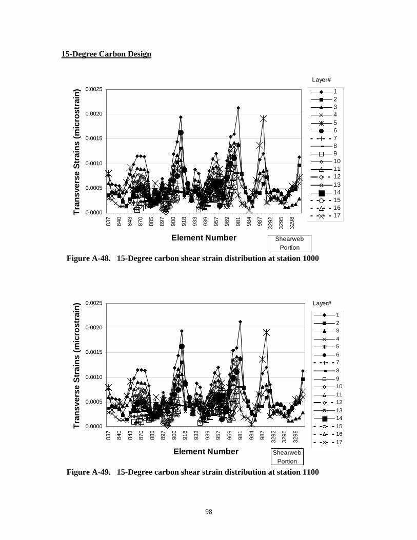
98
15-Degree Carbon Design
0.0000
0.0005
0.0010
0.0015
0.0020
0.0025
837
840
843
870
885
897
900
918
933
939
957
969
981
984
987
3292
3295
3298
Element Number
Tran
sver
se S
trai
ns (m
icro
stra
in) 1
234567891011121314151617
Layer#
Shearweb Portion
Figure A-48. 15-Degree carbon shear strain distribution at station 1000
0.0000
0.0005
0.0010
0.0015
0.0020
0.0025
837
840
843
870
885
897
900
918
933
939
957
969
981
984
987
3292
3295
3298
Element Number
Tran
sver
se S
trai
ns (m
icro
stra
in)
1234567891011121314151617
Layer#
Shearweb Portion
Figure A-49. 15-Degree carbon shear strain distribution at station 1100
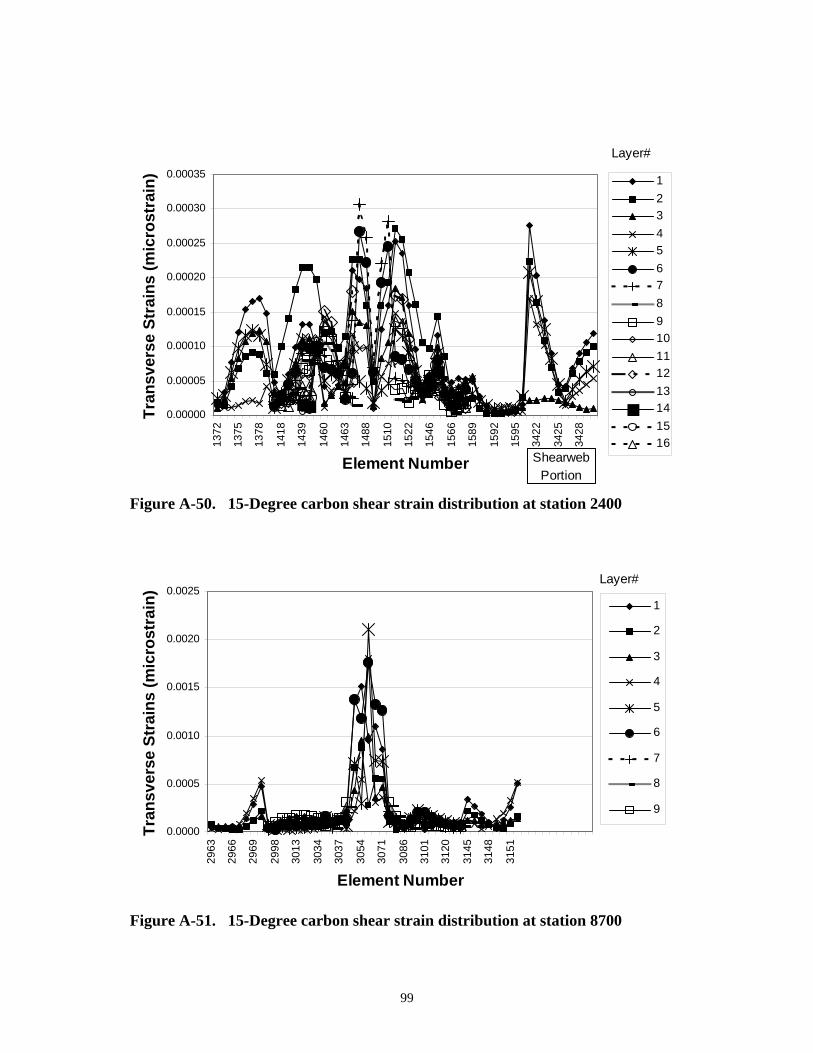
99
0.00000
0.00005
0.00010
0.00015
0.00020
0.00025
0.00030
0.00035
1372
1375
1378
1418
1439
1460
1463
1488
1510
1522
1546
1566
1589
1592
1595
3422
3425
3428
Element Number
Tran
sver
se S
trai
ns (m
icro
stra
in) 1
2345678910111213141516
Layer#
Shearweb Portion
Figure A-50. 15-Degree carbon shear strain distribution at station 2400
0.0000
0.0005
0.0010
0.0015
0.0020
0.0025
2963
2966
2969
2998
3013
3034
3037
3054
3071
3086
3101
3120
3145
3148
3151
Element Number
Tran
sver
se S
trai
ns (m
icro
stra
in)
1
2
3
4
5
6
7
8
9
Layer#
Figure A-51. 15-Degree carbon shear strain distribution at station 8700
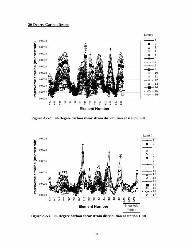
100
20-Degree Carbon Design
0.0000
0.0002
0.0004
0.0006
0.0008
0.0010
0.0012
0.0014
0.0016
0.0018
682
685
688
706
715
736
739
748
760
778
784
802
829
832
835
Element Number
Tran
sver
se S
trai
ns (m
icro
stra
in) 1
2345678910111213141516
Layer#
Figure A-52. 20-Degree carbon shear strain distribution at station 900
0.0000
0.0005
0.0010
0.0015
0.0020
0.0025
837
840
843
870
885
897
900
918
933
939
957
969
981
984
987
3292
3295
3298
Element Number
Tran
sver
se S
trai
ns (m
icro
stra
in) 1
234567891011121314151617
Layer#
Shearweb Portion
Figure A-53. 20-Degree carbon shear strain distribution at station 1000

101
0.00000
0.00005
0.00010
0.00015
0.00020
0.00025
0.00030
0.00035
1372
1375
1378
1418
1439
1460
1463
1488
1510
1522
1546
1566
1589
1592
1595
3422
3425
3428
Element Number
Tran
sver
se S
trai
ns (m
icro
stra
in)
12345678910111213141516
Layer#
Shearweb Portion
Figure A-54. 20-Degree carbon shear strain distribution at station 2400
0.0000
0.0005
0.0010
0.0015
0.0020
0.0025
2963
2966
2969
2998
3013
3034
3037
3054
3071
3086
3101
3120
3145
3148
3151
Element Number
Tran
sver
se S
trai
ns (m
icro
stra
in)
1
2
3
4
5
6
7
8
9
Layer#
Figure A-55. 20-Degree carbon shear strain distribution at station 8700
102
APPENDIX B: PARKED LOAD AXIAL, TRANSVERSE AND SHEAR STRAIN LAYER WISE DISTRIBUTIONS
List of Figures for Appendix B Figure B-1. Baseline axial strain distribution at station 800 ...................................... 104 Figure B-2. Baseline axial strain distribution at station 1200 .................................... 104 Figure B-3. Baseline axial strain distribution at station 2400 .................................... 105 Figure B-4. Baseline axial strain distribution at station 8700 .................................... 105 Figure B-5. 0-Degree carbon axial strain distribution at station 1000 ....................... 106 Figure B-6. 0-Degree carbon axial strain distribution at station 1300 ....................... 106 Figure B-7. 0-Degree carbon axial strain distribution at station 2400 ....................... 107 Figure B-8. 0-Degree carbon axial strain distribution at station 8700 ....................... 107 Figure B-9. 15-Degree carbon axial strain distribution at station 1000 ..................... 108 Figure B-10. 15-Degree carbon axial strain distribution at station 1100 ................. 108 Figure B-11. 15-Degree carbon axial strain distribution at station 2400 ................. 109 Figure B-12. 15-Degree carbon axial strain distribution at station 8700 ................. 109 Figure B-13. 20-Degree carbon axial strain distribution at station 900 ................... 110 Figure B-14. 20-Degree carbon axial strain distribution at station 1000 ................. 110 Figure B-15. 20-Degree carbon axial strain distribution at station 2400 ................. 111 Figure B-16. 20-Degree carbon axial strain distribution at station 8700 ................. 111 Figure B-17. Baseline transverse strain distribution at station 800.......................... 112 Figure B-18. Baseline transverse strain distribution at station 1200........................ 112 Figure B-19. Baseline transverse strain distribution at station 2400........................ 113 Figure B-20. Baseline transverse strain distribution at station 8700........................ 113 Figure B-21. 0-Degree carbon transverse strain distribution at station 1000........... 114 Figure B-22. 0-Degree carbon transverse strain distribution at station 1300........... 114 Figure B-23. 0-Degree carbon transverse strain distribution at station 2400........... 115 Figure B-24. 0-Degree carbon transverse strain distribution at station 8700........... 115 Figure B-25. 15-Degree carbon transverse strain distribution at station 1000......... 116 Figure B-26. 15-Degree carbon transverse strain distribution at station 1100......... 116 Figure B-27. 15-Degree carbon transverse strain distribution at station 2400......... 117 Figure B-28. 15-Degree carbon transverse strain distribution at station 8700......... 117 Figure B-29. 20-Degree carbon transverse strain distribution at station 900........... 118 Figure B-30. 20-Degree carbon transverse strain distribution at station 1000......... 118 Figure B-31. 20-Degree carbon transverse strain distribution at station 2400......... 119 Figure B-32. 20-Degree carbon transverse strain distribution at station 8700......... 119 Figure B-33. Baseline shear strain distribution at station 800 ................................. 120 Figure B-34. Baseline shear strain distribution at station 1200 ............................... 120 Figure B-35. Baseline shear strain distribution at station 2400 ............................... 121 Figure B-36. Baseline shear strain distribution at station 8700 ............................... 121 Figure B-37. 0-Degree carbon shear strain distribution at station 1000 .................. 122 Figure B-38. 0-Degree carbon shear strain distribution at station 1300 .................. 122 Figure B-39. 0-Degree carbon shear strain distribution at station 2400 .................. 123 Figure B-40. 0-Degree carbon shear strain distribution at station 8700 .................. 123 Figure B-41. 15-Degree carbon shear strain distribution at station 1000 ................ 124
103
Figure B-42. 15-Degree carbon shear strain distribution at station 1100 ................ 124 Figure B-43. 15-Degree carbon shear strain distribution at station 2400 ................ 125 Figure B-44. 15-Degree carbon shear strain distribution at station 8700 ................ 125 Figure B-45. 20-Degree carbon shear strain distribution at station 900 .................. 126 Figure B-46. 20-Degree carbon shear strain distribution at station 1000 ................ 126 Figure B-47. 20-Degree carbon shear strain distribution at station 2400 ................ 127 Figure B-48. 20-Degree carbon shear strain distribution at station 8700 ................ 127
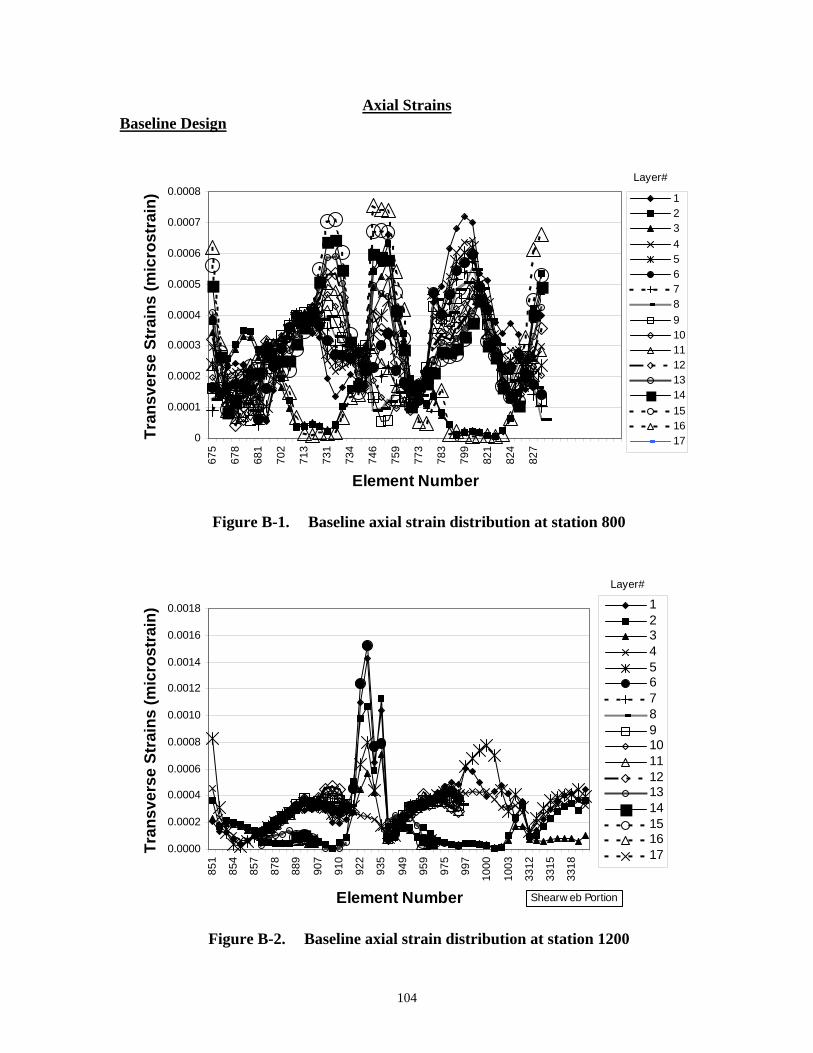
104
Axial Strains Baseline Design
0
0.0001
0.0002
0.0003
0.0004
0.0005
0.0006
0.0007
0.0008
675
678
681
702
713
731
734
746
759
773
783
799
821
824
827
Element Number
Tran
sver
se S
trai
ns (m
icro
stra
in) 1
234567891011121314151617
Layer#
Figure B-1. Baseline axial strain distribution at station 800
0.0000
0.0002
0.0004
0.0006
0.0008
0.0010
0.0012
0.0014
0.0016
0.0018
851
854
857
878
889
907
910
922
935
949
959
975
997
1000
1003
3312
3315
3318
Element Number
Tran
sver
se S
trai
ns (m
icro
stra
in) 1
234567891011121314151617
Layer#
Shearw eb Portion
Figure B-2. Baseline axial strain distribution at station 1200
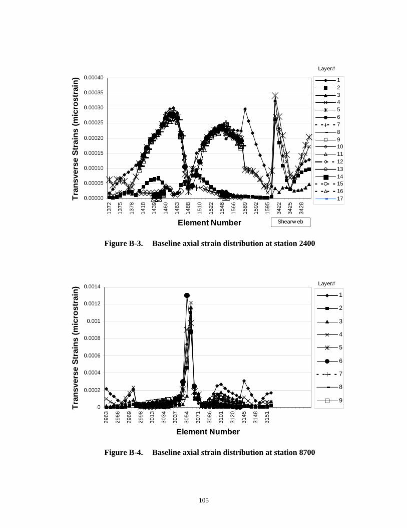
105
0.00000
0.00005
0.00010
0.00015
0.00020
0.00025
0.00030
0.00035
0.00040
1372
1375
1378
1418
1439
1460
1463
1488
1510
1522
1546
1566
1589
1592
1595
3422
3425
3428
Element Number
Tran
sver
se S
trai
ns (m
icro
stra
in) 1
234567891011121314151617
Layer#
Shearw eb
Figure B-3. Baseline axial strain distribution at station 2400
0
0.0002
0.0004
0.0006
0.0008
0.001
0.0012
0.0014
2963
2966
2969
2998
3013
3034
3037
3054
3071
3086
3101
3120
3145
3148
3151
Element Number
Tran
sver
se S
trai
ns (m
icro
stra
in)
1
2
3
4
5
6
7
8
9
Layer#
Figure B-4. Baseline axial strain distribution at station 8700
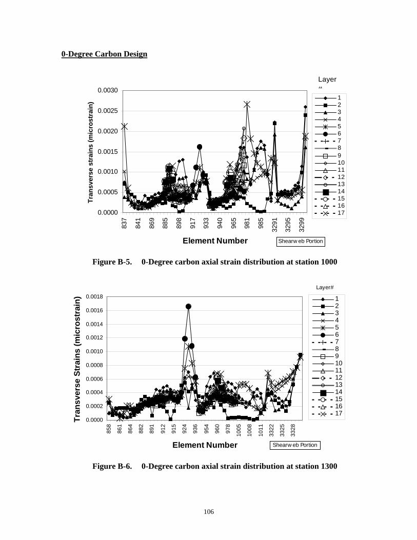
106
0-Degree Carbon Design
0.0000
0.0005
0.0010
0.0015
0.0020
0.0025
0.0030
837
841
869
885
898
917
933
940
965
981
985
3291
3295
3299
Element Number
Tran
sver
se s
trai
ns (m
icro
stra
in) 1
234567891011121314151617
Layer#
Shearw eb Portion
Figure B-5. 0-Degree carbon axial strain distribution at station 1000
0.0000
0.0002
0.0004
0.0006
0.0008
0.0010
0.0012
0.0014
0.0016
0.0018
858
861
864
882
891
912
915
924
936
954
960
978
1005
1008
1011
3322
3325
3328
Element Number
Tran
sver
se S
trai
ns (m
icro
stra
in) 1
234567891011121314151617
Layer#
Shearw eb Portion
Figure B-6. 0-Degree carbon axial strain distribution at station 1300
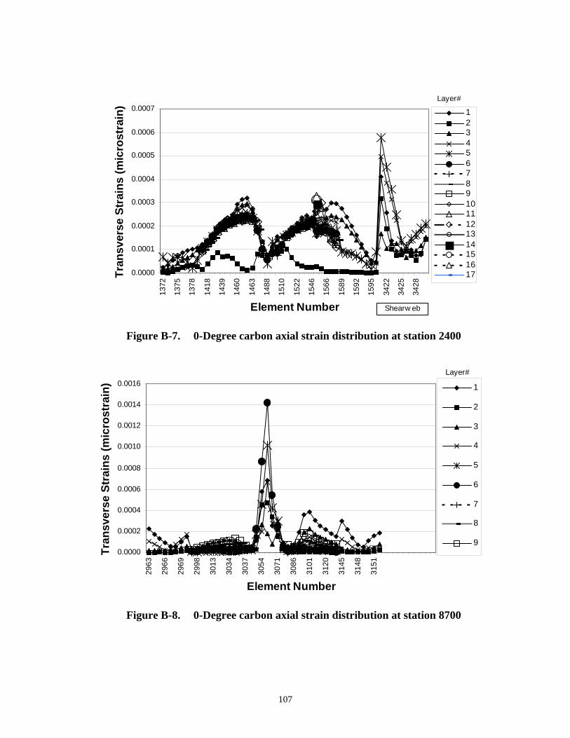
107
0.0000
0.0001
0.0002
0.0003
0.0004
0.0005
0.0006
0.0007
1372
1375
1378
1418
1439
1460
1463
1488
1510
1522
1546
1566
1589
1592
1595
3422
3425
3428
Element Number
Tran
sver
se S
trai
ns (m
icro
stra
in) 1
234567891011121314151617
Layer#
Shearw eb
Figure B-7. 0-Degree carbon axial strain distribution at station 2400
0.0000
0.0002
0.0004
0.0006
0.0008
0.0010
0.0012
0.0014
0.0016
2963
2966
2969
2998
3013
3034
3037
3054
3071
3086
3101
3120
3145
3148
3151
Element Number
Tran
sver
se S
trai
ns (m
icro
stra
in) 1
2
3
4
5
6
7
8
9
Layer#
Figure B-8. 0-Degree carbon axial strain distribution at station 8700
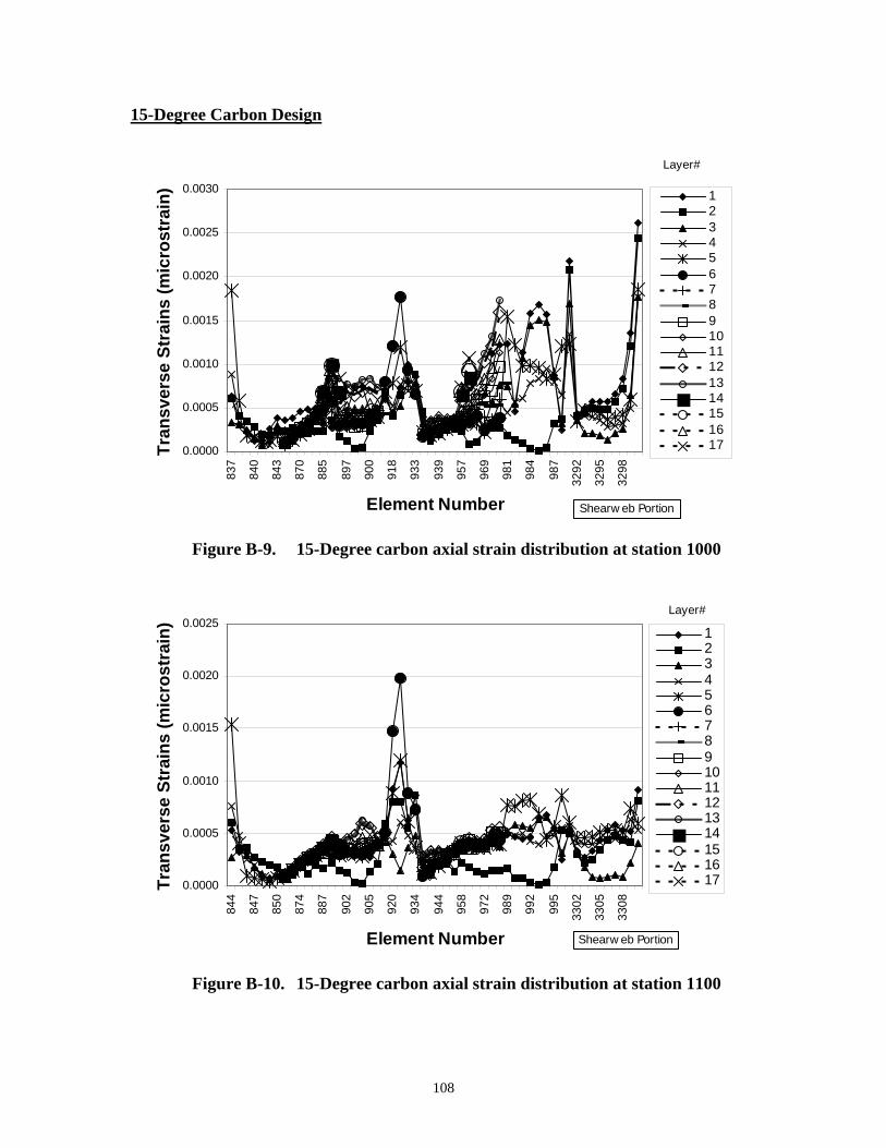
108
15-Degree Carbon Design
0.0000
0.0005
0.0010
0.0015
0.0020
0.0025
0.0030
837
840
843
870
885
897
900
918
933
939
957
969
981
984
987
3292
3295
3298
Element Number
Tran
sver
se S
trai
ns (m
icro
stra
in) 1
234567891011121314151617
Layer#
Shearw eb Portion
Figure B-9. 15-Degree carbon axial strain distribution at station 1000
0.0000
0.0005
0.0010
0.0015
0.0020
0.0025
844
847
850
874
887
902
905
920
934
944
958
972
989
992
995
3302
3305
3308
Element Number
Tran
sver
se S
trai
ns (m
icro
stra
in) 1
234567891011121314151617
Layer#
Shearw eb Portion
Figure B-10. 15-Degree carbon axial strain distribution at station 1100
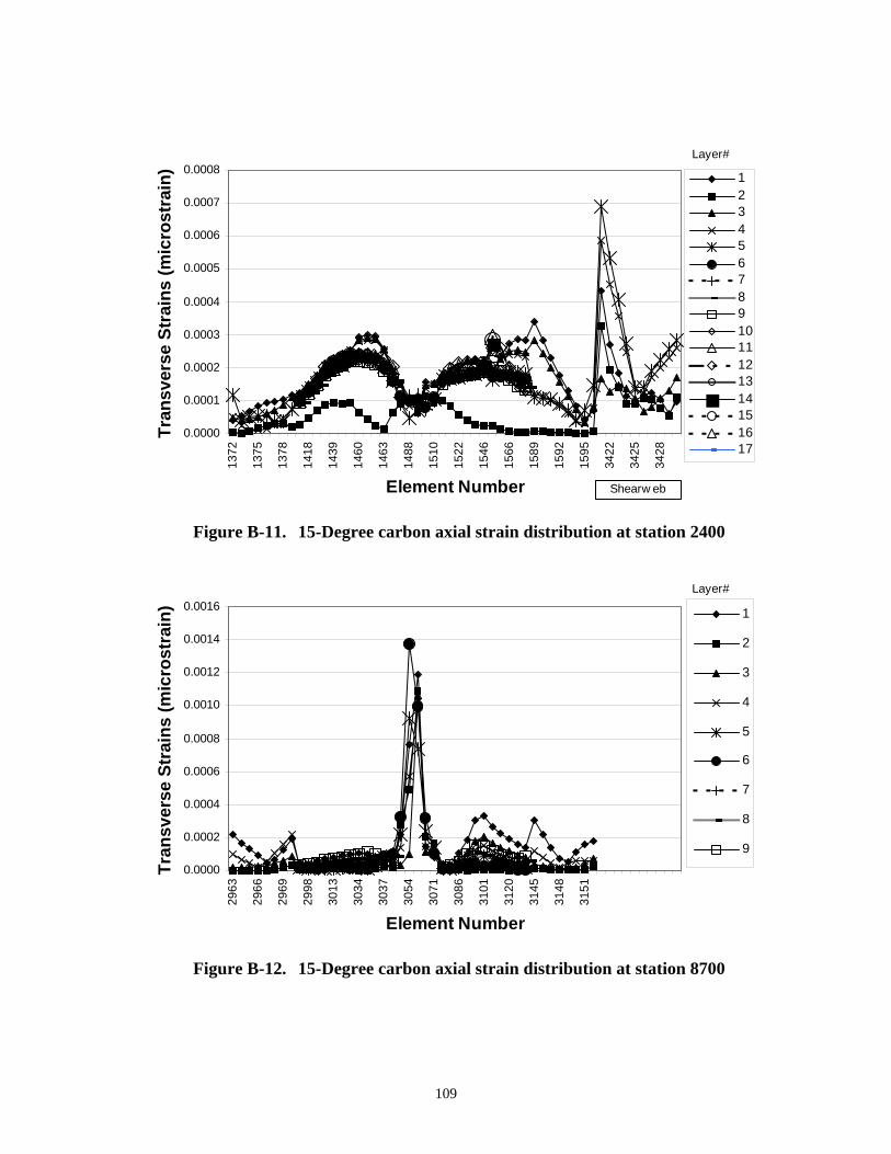
109
0.0000
0.0001
0.0002
0.0003
0.0004
0.0005
0.0006
0.0007
0.0008
1372
1375
1378
1418
1439
1460
1463
1488
1510
1522
1546
1566
1589
1592
1595
3422
3425
3428
Element Number
Tran
sver
se S
trai
ns (m
icro
stra
in) 1
234567891011121314151617
Layer#
Shearw eb
Figure B-11. 15-Degree carbon axial strain distribution at station 2400
0.0000
0.0002
0.0004
0.0006
0.0008
0.0010
0.0012
0.0014
0.0016
2963
2966
2969
2998
3013
3034
3037
3054
3071
3086
3101
3120
3145
3148
3151
Element Number
Tran
sver
se S
trai
ns (m
icro
stra
in) 1
2
3
4
5
6
7
8
9
Layer#
Figure B-12. 15-Degree carbon axial strain distribution at station 8700
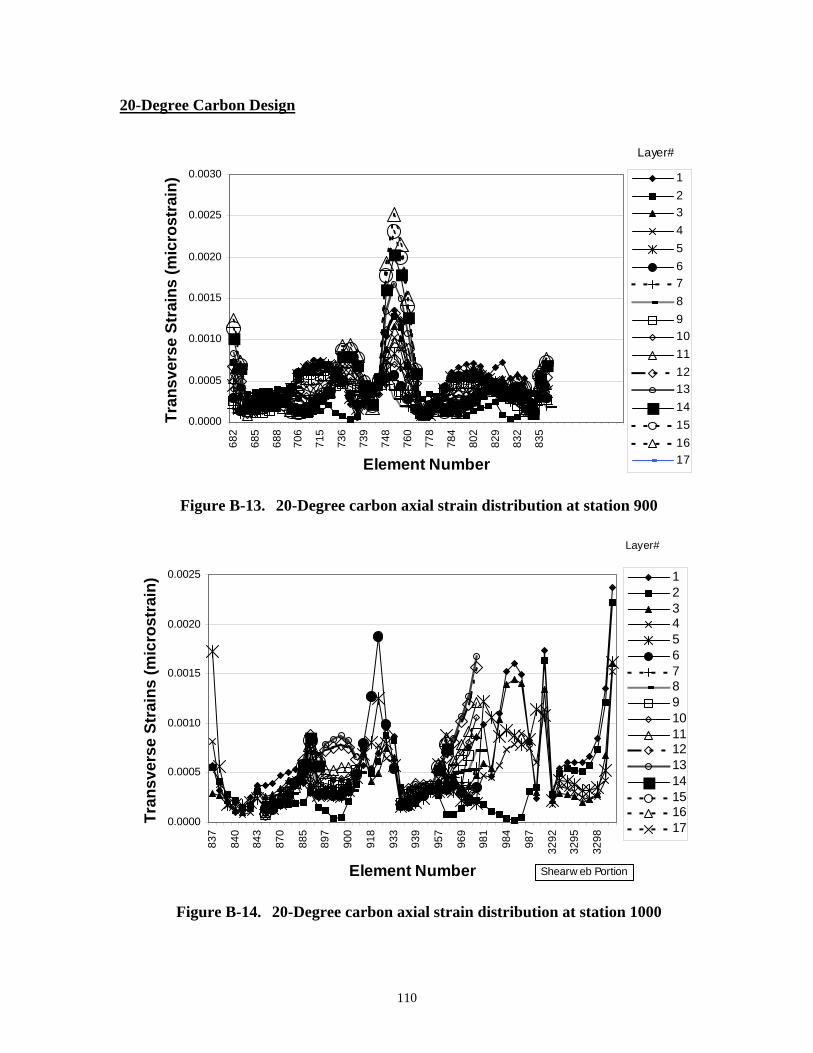
110
20-Degree Carbon Design
0.0000
0.0005
0.0010
0.0015
0.0020
0.0025
0.0030
682
685
688
706
715
736
739
748
760
778
784
802
829
832
835
Element Number
Tran
sver
se S
trai
ns (m
icro
stra
in) 1
234567891011121314151617
Layer#
Figure B-13. 20-Degree carbon axial strain distribution at station 900
0.0000
0.0005
0.0010
0.0015
0.0020
0.0025
837
840
843
870
885
897
900
918
933
939
957
969
981
984
987
3292
3295
3298
Element Number
Tran
sver
se S
trai
ns (m
icro
stra
in) 1
234567891011121314151617
Layer#
Shearw eb Portion
Figure B-14. 20-Degree carbon axial strain distribution at station 1000
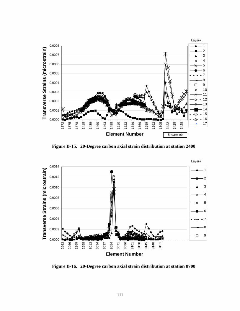
111
0.0000
0.0001
0.0002
0.0003
0.0004
0.0005
0.0006
0.0007
0.0008
1372
1375
1378
1418
1439
1460
1463
1488
1510
1522
1546
1566
1589
1592
1595
3422
3425
3428
Element Number
Tran
sver
se S
trai
ns (m
icro
stra
in) 1
234567891011121314151617
Layer#
Shearw eb
Figure B-15. 20-Degree carbon axial strain distribution at station 2400
0.0000
0.0002
0.0004
0.0006
0.0008
0.0010
0.0012
0.0014
2963
2966
2969
2998
3013
3034
3037
3054
3071
3086
3101
3120
3145
3148
3151
Element Number
Tran
sver
se S
trai
ns (m
icro
stra
in) 1
2
3
4
5
6
7
8
9
Layer#
Figure B-16. 20-Degree carbon axial strain distribution at station 8700
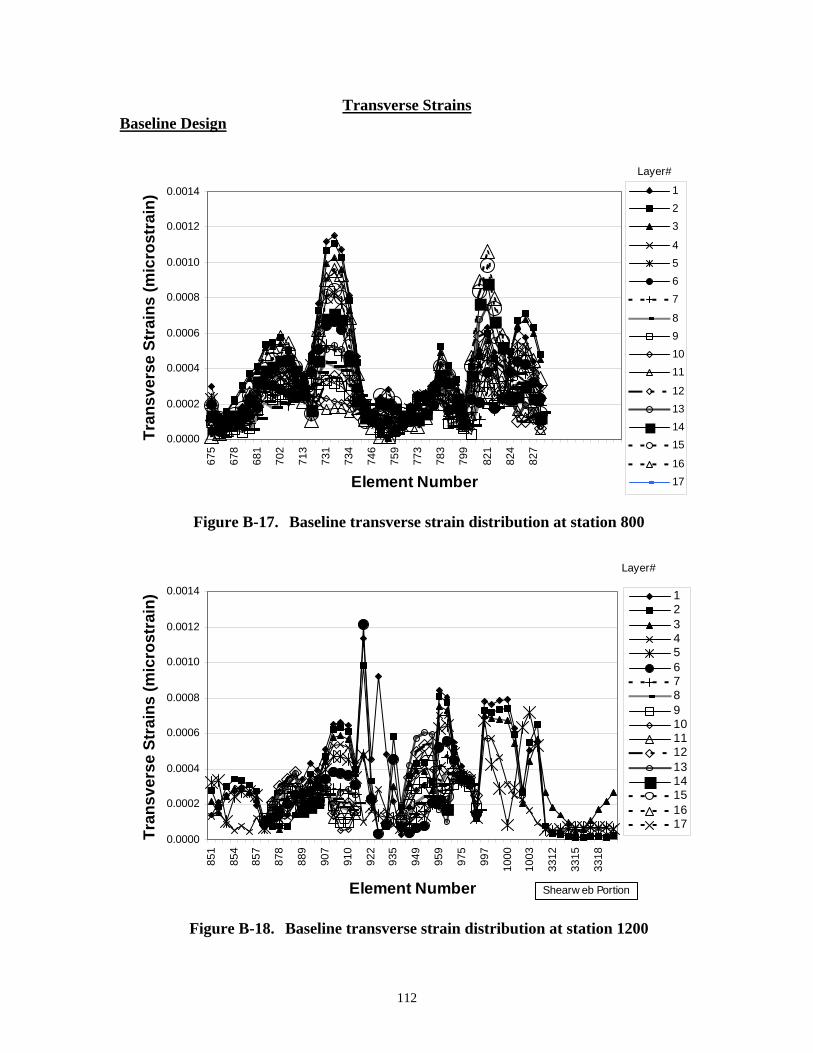
112
Transverse Strains Baseline Design
0.0000
0.0002
0.0004
0.0006
0.0008
0.0010
0.0012
0.0014
675
678
681
702
713
731
734
746
759
773
783
799
821
824
827
Element Number
Tran
sver
se S
trai
ns (m
icro
stra
in) 1
23
4567
891011
12131415
1617
Layer#
Figure B-17. Baseline transverse strain distribution at station 800
0.0000
0.0002
0.0004
0.0006
0.0008
0.0010
0.0012
0.0014
851
854
857
878
889
907
910
922
935
949
959
975
997
1000
1003
3312
3315
3318
Element Number
Tran
sver
se S
trai
ns (m
icro
stra
in) 1
234567891011121314151617
Layer#
Shearw eb Portion
Figure B-18. Baseline transverse strain distribution at station 1200
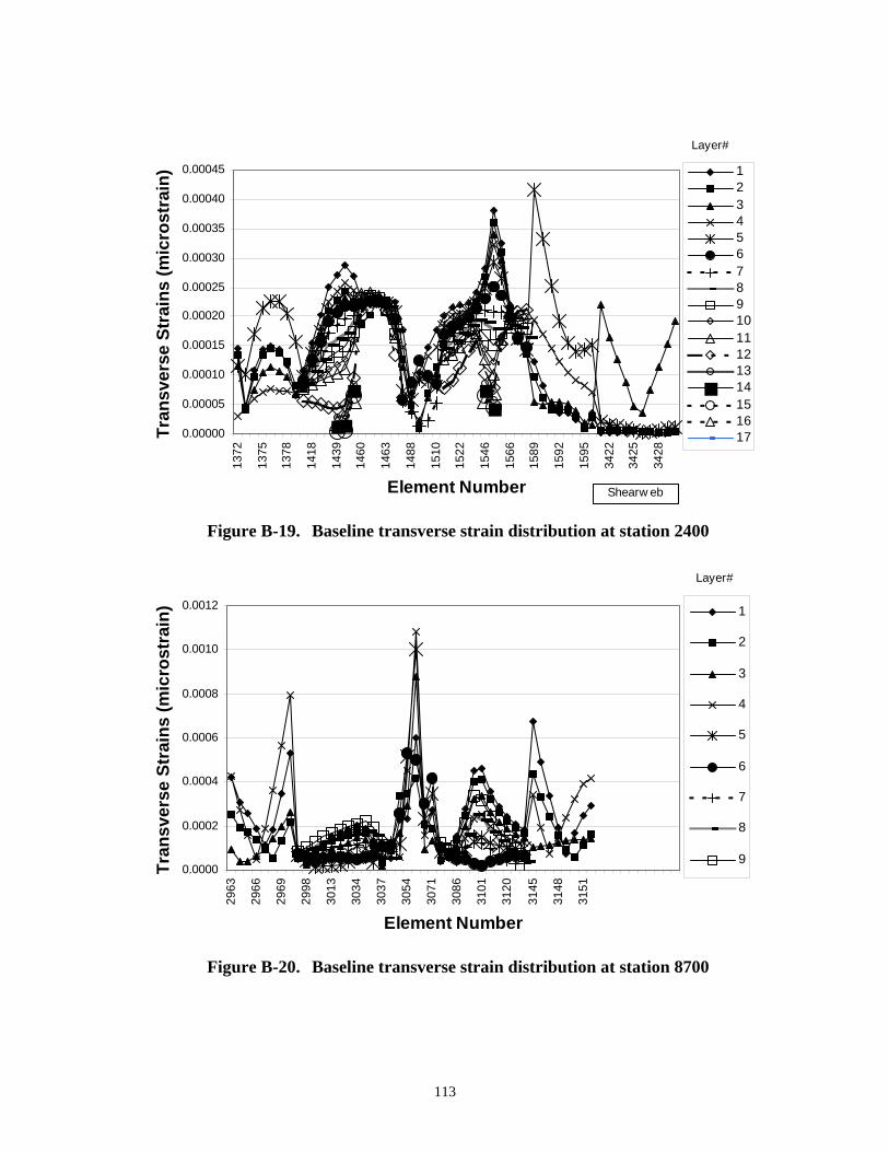
113
0.00000
0.00005
0.00010
0.00015
0.00020
0.00025
0.00030
0.00035
0.00040
0.00045
1372
1375
1378
1418
1439
1460
1463
1488
1510
1522
1546
1566
1589
1592
1595
3422
3425
3428
Element Number
Tran
sver
se S
trai
ns (m
icro
stra
in) 1
234567891011121314151617
Layer#
Shearw eb
Figure B-19. Baseline transverse strain distribution at station 2400
0.0000
0.0002
0.0004
0.0006
0.0008
0.0010
0.0012
2963
2966
2969
2998
3013
3034
3037
3054
3071
3086
3101
3120
3145
3148
3151
Element Number
Tran
sver
se S
trai
ns (m
icro
stra
in) 1
2
3
4
5
6
7
8
9
Layer#
Figure B-20. Baseline transverse strain distribution at station 8700
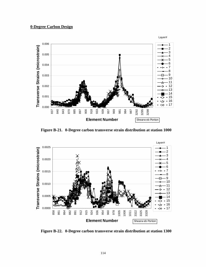
114
0-Degree Carbon Design
0.000
0.001
0.002
0.003
0.004
0.005
0.006
837
840
843
870
885
897
900
918
933
939
957
969
981
984
987
3292
3295
3298
Element Number
Tran
sver
se S
trai
ns (m
icro
stra
in) 1
234567891011121314151617
Layer#
Shearw eb Portion
Figure B-21. 0-Degree carbon transverse strain distribution at station 1000
0.0000
0.0005
0.0010
0.0015
0.0020
0.0025
858
861
864
882
891
912
915
924
936
954
960
978
1005
1008
1011
3322
3325
3328
Element Number
Tran
sver
se S
trai
ns (m
icro
stra
in) 1
234567891011121314151617
Layer#
Shearw eb Portion
Figure B-22. 0-Degree carbon transverse strain distribution at station 1300
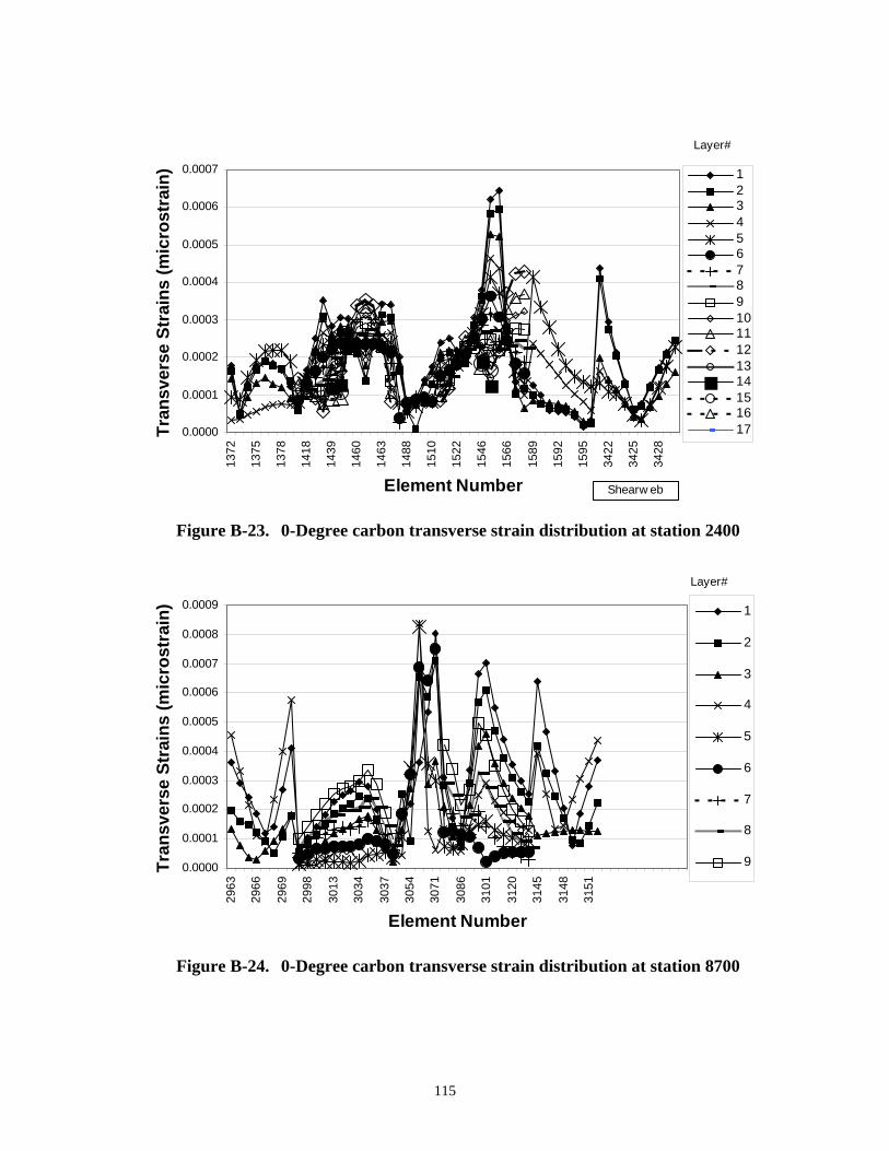
115
0.0000
0.0001
0.0002
0.0003
0.0004
0.0005
0.0006
0.0007
1372
1375
1378
1418
1439
1460
1463
1488
1510
1522
1546
1566
1589
1592
1595
3422
3425
3428
Element Number
Tran
sver
se S
trai
ns (m
icro
stra
in) 1
234567891011121314151617
Layer#
Shearw eb
Figure B-23. 0-Degree carbon transverse strain distribution at station 2400
0.0000
0.0001
0.0002
0.0003
0.0004
0.0005
0.0006
0.0007
0.0008
0.0009
2963
2966
2969
2998
3013
3034
3037
3054
3071
3086
3101
3120
3145
3148
3151
Element Number
Tran
sver
se S
trai
ns (m
icro
stra
in) 1
2
3
4
5
6
7
8
9
Layer#
Figure B-24. 0-Degree carbon transverse strain distribution at station 8700
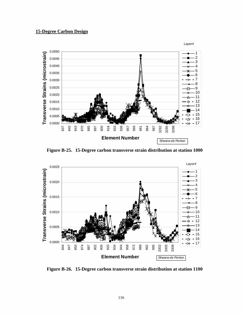
116
15-Degree Carbon Design
0.0000
0.0005
0.0010
0.0015
0.0020
0.0025
0.0030
0.0035
0.0040
0.0045
0.0050
837
840
843
870
885
897
900
918
933
939
957
969
981
984
987
3292
3295
3298
Element Number
Tran
sver
se S
trai
ns (m
icro
stra
in) 1
234567891011121314151617
Layer#
Shearw eb Portion
Figure B-25. 15-Degree carbon transverse strain distribution at station 1000
0.0000
0.0005
0.0010
0.0015
0.0020
0.0025
844
847
850
874
887
902
905
920
934
944
958
972
989
992
995
3302
3305
3308
Element Number
Tran
sver
se S
trai
ns (m
icro
stra
in)
1234567891011121314151617
Layer#
Shearw eb Portion
Figure B-26. 15-Degree carbon transverse strain distribution at station 1100
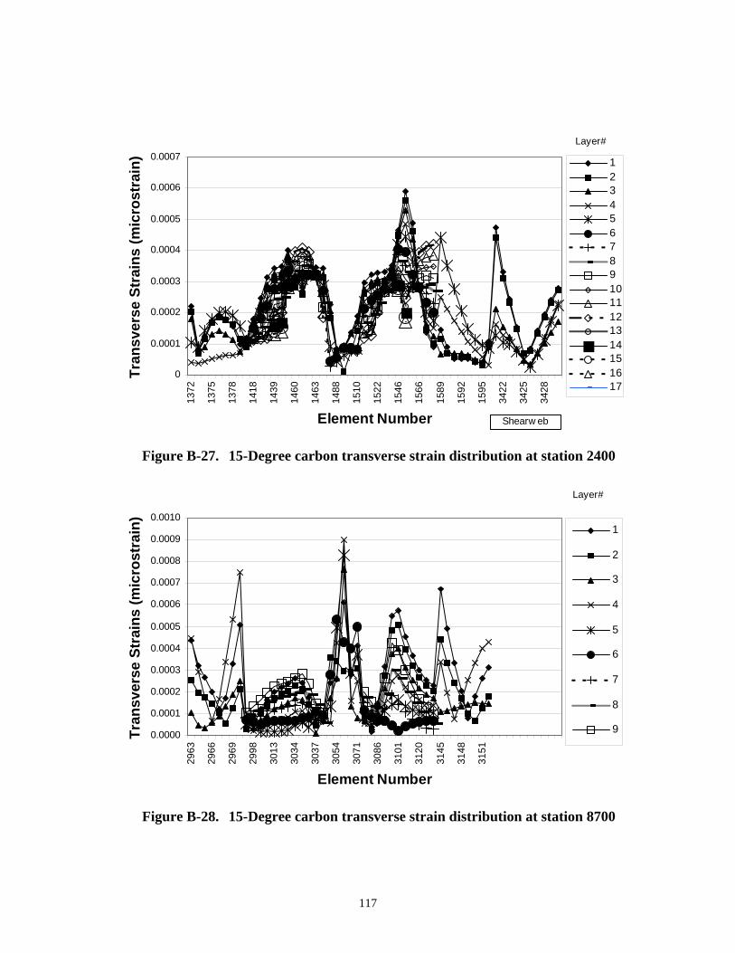
117
0
0.0001
0.0002
0.0003
0.0004
0.0005
0.0006
0.0007
1372
1375
1378
1418
1439
1460
1463
1488
1510
1522
1546
1566
1589
1592
1595
3422
3425
3428
Element Number
Tran
sver
se S
trai
ns (m
icro
stra
in) 1
234567891011121314151617
Layer#
Shearw eb
Figure B-27. 15-Degree carbon transverse strain distribution at station 2400
0.0000
0.0001
0.0002
0.0003
0.0004
0.0005
0.0006
0.0007
0.0008
0.0009
0.0010
2963
2966
2969
2998
3013
3034
3037
3054
3071
3086
3101
3120
3145
3148
3151
Element Number
Tran
sver
se S
trai
ns (m
icro
stra
in)
1
2
3
4
5
6
7
8
9
Layer#
Figure B-28. 15-Degree carbon transverse strain distribution at station 8700

118
20-Degree Carbon Design
0.0000
0.0005
0.0010
0.0015
0.0020
0.0025
0.0030
0.0035
0.0040
682
685
688
706
715
736
739
748
760
778
784
802
829
832
835
Element Number
Tran
sver
se S
trai
ns (m
icro
stra
in) 1
234567891011121314151617
Layer#
Figure B-29. 20-Degree carbon transverse strain distribution at station 900
0.0000
0.0005
0.0010
0.0015
0.0020
0.0025
0.0030
0.0035
0.0040
0.0045
0.0050
837
840
843
870
885
897
900
918
933
939
957
969
981
984
987
3292
3295
3298
Element Number
Tran
sver
se S
trai
ns (m
icro
stra
in) 1
234567891011121314151617
Layer#
Shearw eb Portion
Figure B-30. 20-Degree carbon transverse strain distribution at station 1000
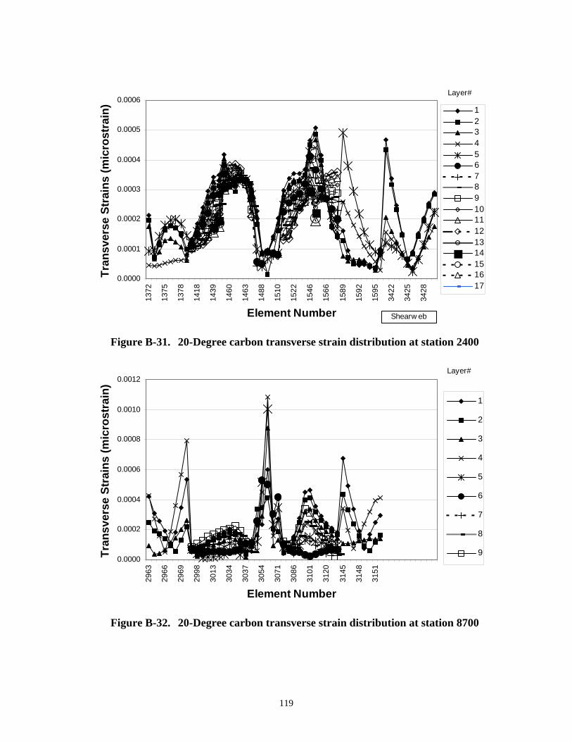
119
0.0000
0.0001
0.0002
0.0003
0.0004
0.0005
0.0006
1372
1375
1378
1418
1439
1460
1463
1488
1510
1522
1546
1566
1589
1592
1595
3422
3425
3428
Element Number
Tran
sver
se S
trai
ns (m
icro
stra
in) 1
234567891011121314151617
Layer#
Shearw eb
Figure B-31. 20-Degree carbon transverse strain distribution at station 2400
0.0000
0.0002
0.0004
0.0006
0.0008
0.0010
0.0012
2963
2966
2969
2998
3013
3034
3037
3054
3071
3086
3101
3120
3145
3148
3151
Element Number
Tran
sver
se S
trai
ns (m
icro
stra
in)
1
2
3
4
5
6
7
8
9
Layer#
Figure B-32. 20-Degree carbon transverse strain distribution at station 8700
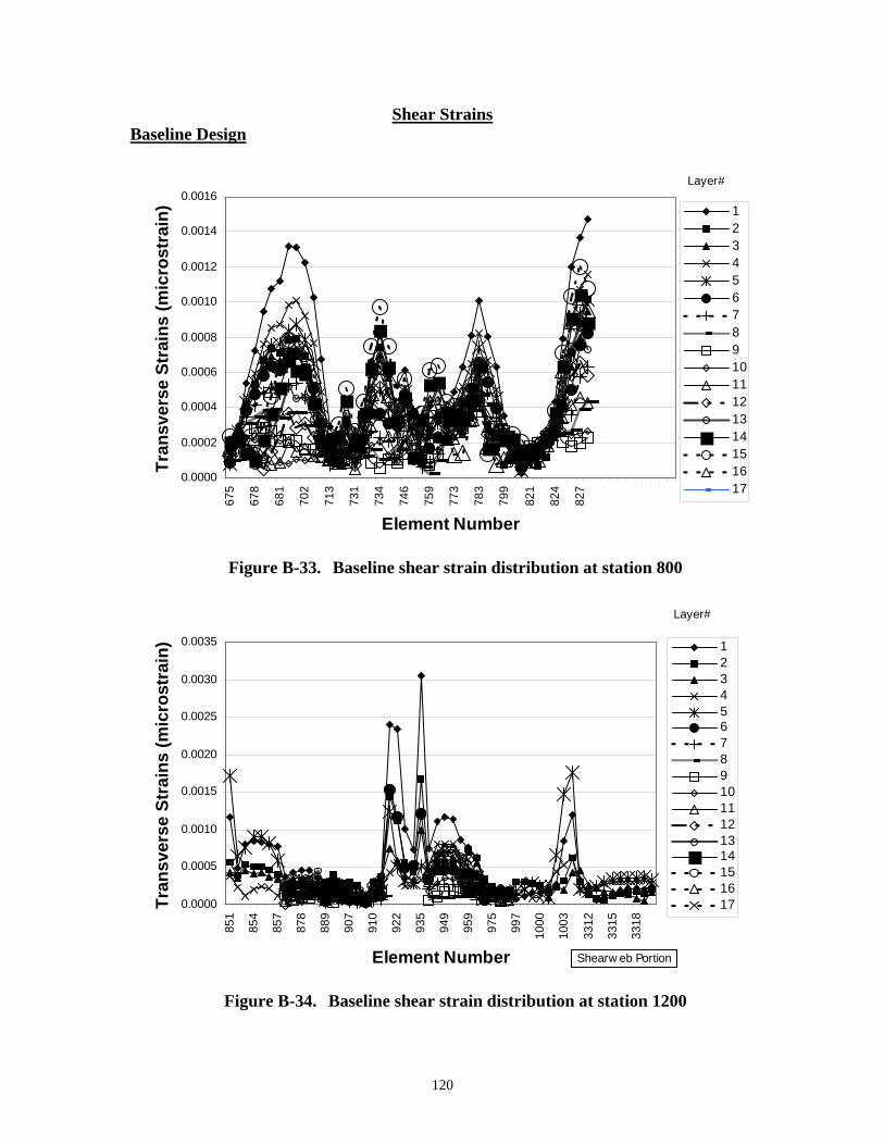
120
Shear Strains Baseline Design
0.0000
0.0002
0.0004
0.0006
0.0008
0.0010
0.0012
0.0014
0.0016
675
678
681
702
713
731
734
746
759
773
783
799
821
824
827
Element Number
Tran
sver
se S
trai
ns (m
icro
stra
in) 1
234567891011121314151617
Layer#
Figure B-33. Baseline shear strain distribution at station 800
0.0000
0.0005
0.0010
0.0015
0.0020
0.0025
0.0030
0.0035
851
854
857
878
889
907
910
922
935
949
959
975
997
1000
1003
3312
3315
3318
Element Number
Tran
sver
se S
trai
ns (m
icro
stra
in) 1
234567891011121314151617
Shearw eb Portion
Layer#
Figure B-34. Baseline shear strain distribution at station 1200
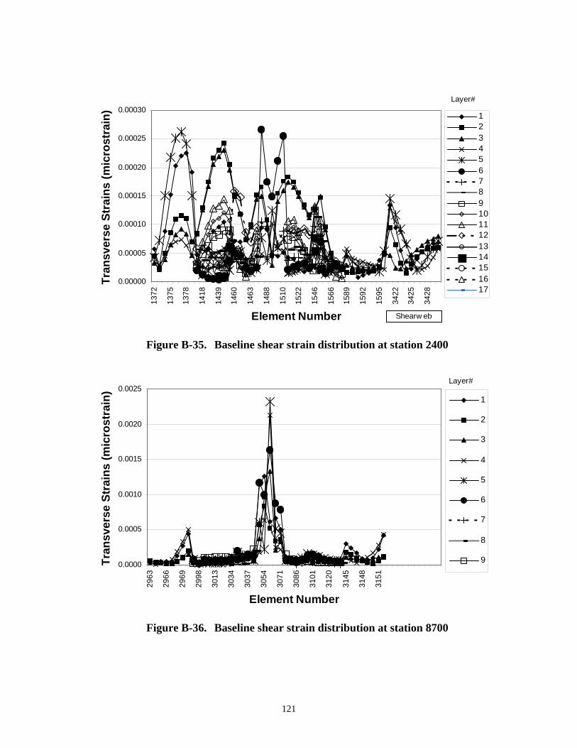
121
0.00000
0.00005
0.00010
0.00015
0.00020
0.00025
0.00030
1372
1375
1378
1418
1439
1460
1463
1488
1510
1522
1546
1566
1589
1592
1595
3422
3425
3428
Element Number
Tran
sver
se S
trai
ns (m
icro
stra
in) 1
234567891011121314151617
Shearw eb
Layer#
Figure B-35. Baseline shear strain distribution at station 2400
0.0000
0.0005
0.0010
0.0015
0.0020
0.0025
2963
2966
2969
2998
3013
3034
3037
3054
3071
3086
3101
3120
3145
3148
3151
Element Number
Tran
sver
se S
trai
ns (m
icro
stra
in)
1
2
3
4
5
6
7
8
9
Layer#
Figure B-36. Baseline shear strain distribution at station 8700
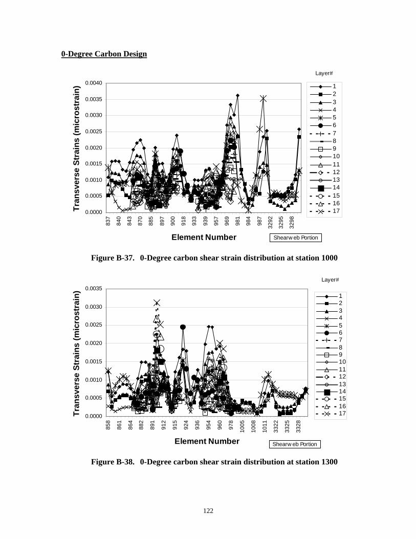
122
0-Degree Carbon Design
0.0000
0.0005
0.0010
0.0015
0.0020
0.0025
0.0030
0.0035
0.0040
837
840
843
870
885
897
900
918
933
939
957
969
981
984
987
3292
3295
3298
Element Number
Tran
sver
se S
trai
ns (m
icro
stra
in) 1
234567891011121314151617
Shearw eb Portion
Layer#
Figure B-37. 0-Degree carbon shear strain distribution at station 1000
0.0000
0.0005
0.0010
0.0015
0.0020
0.0025
0.0030
0.0035
858
861
864
882
891
912
915
924
936
954
960
978
1005
1008
1011
3322
3325
3328
Element Number
Tran
sver
se S
trai
ns (m
icro
stra
in)
1234567891011121314151617
Shearw eb Portion
Layer#
Figure B-38. 0-Degree carbon shear strain distribution at station 1300

123
0.00000
0.00005
0.00010
0.00015
0.00020
0.00025
0.00030
0.00035
0.00040
1372
1375
1378
1418
1439
1460
1463
1488
1510
1522
1546
1566
1589
1592
1595
3422
3425
3428
Element Number
Tran
sver
se S
trai
ns (m
icro
stra
in) 1
234567891011121314151617
Shearw eb
Layer#
Figure B-39. 0-Degree carbon shear strain distribution at station 2400
0.0000
0.0005
0.0010
0.0015
0.0020
0.0025
2963
2966
2969
2998
3013
3034
3037
3054
3071
3086
3101
3120
3145
3148
3151
Element Number
Tran
sver
se S
trai
ns (m
icro
stra
in)
1
2
3
4
5
6
7
8
9
Layer#
Figure B-40. 0-Degree carbon shear strain distribution at station 8700
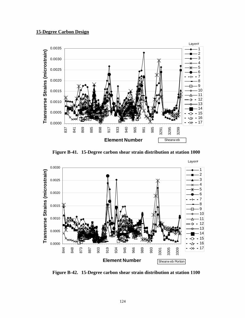
124
15-Degree Carbon Design
0.0000
0.0005
0.0010
0.0015
0.0020
0.0025
0.0030
0.0035
837
841
869
885
898
917
933
940
965
981
985
3291
3295
3299
Element Number
Tran
sver
se S
trai
ns (m
icro
stra
in) 1
234567891011121314151617
Shearw eb
Layer#
Figure B-41. 15-Degree carbon shear strain distribution at station 1000
0.0000
0.0005
0.0010
0.0015
0.0020
0.0025
0.0030
844
848
873
887
903
919
934
945
966
989
993
3301
3305
3309
Element Number
Tran
sver
se S
trai
ns (m
icro
stra
in) 1
234567891011121314151617
Shearw eb Portion
Layer#
Figure B-42. 15-Degree carbon shear strain distribution at station 1100
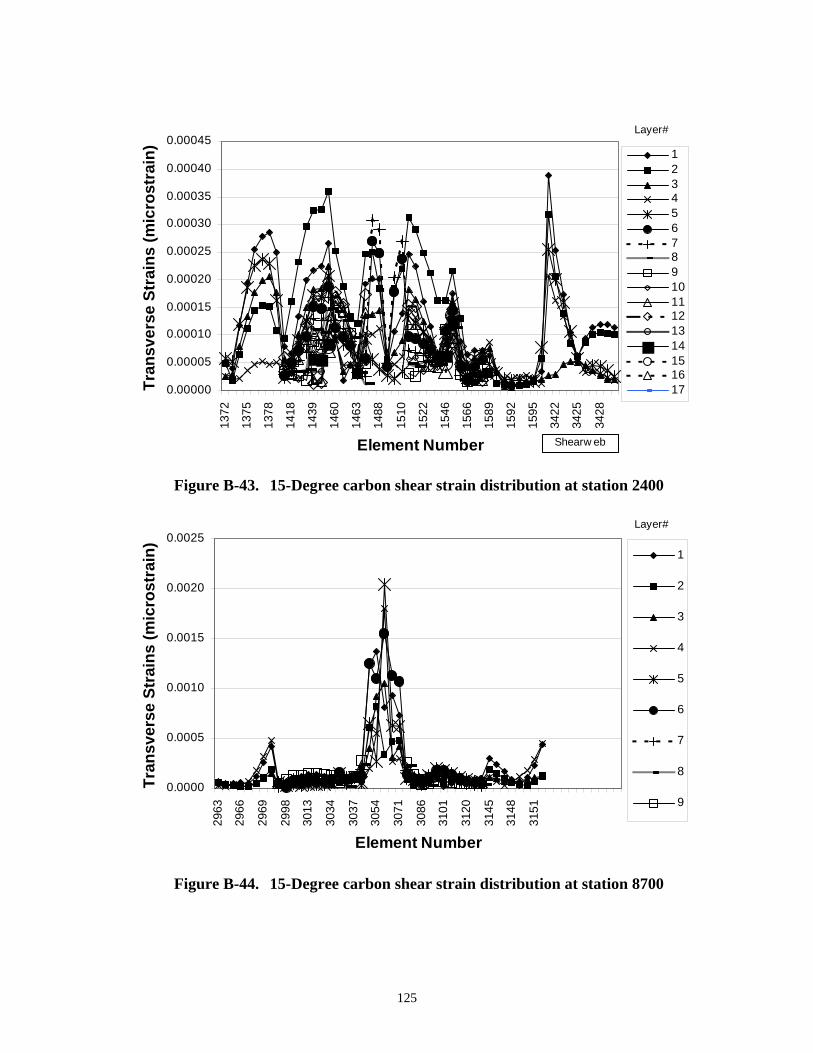
125
0.00000
0.00005
0.00010
0.00015
0.00020
0.00025
0.00030
0.00035
0.00040
0.00045
1372
1375
1378
1418
1439
1460
1463
1488
1510
1522
1546
1566
1589
1592
1595
3422
3425
3428
Element Number
Tran
sver
se S
trai
ns (m
icro
stra
in) 1
234567891011121314151617
Shearw eb
Layer#
Figure B-43. 15-Degree carbon shear strain distribution at station 2400
0.0000
0.0005
0.0010
0.0015
0.0020
0.0025
2963
2966
2969
2998
3013
3034
3037
3054
3071
3086
3101
3120
3145
3148
3151
Element Number
Tran
sver
se S
trai
ns (m
icro
stra
in)
1
2
3
4
5
6
7
8
9
Layer#
Figure B-44. 15-Degree carbon shear strain distribution at station 8700
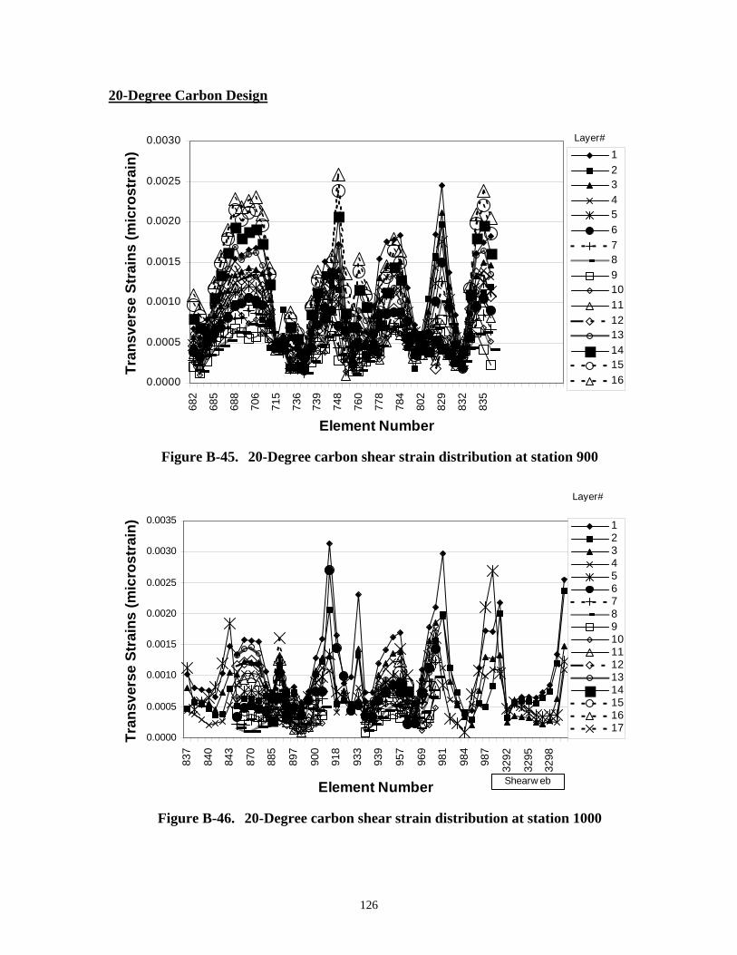
126
20-Degree Carbon Design
0.0000
0.0005
0.0010
0.0015
0.0020
0.0025
0.0030
682
685
688
706
715
736
739
748
760
778
784
802
829
832
835
Element Number
Tran
sver
se S
trai
ns (m
icro
stra
in) 1
2345678910111213141516
Layer#
Figure B-45. 20-Degree carbon shear strain distribution at station 900
0.0000
0.0005
0.0010
0.0015
0.0020
0.0025
0.0030
0.0035
837
840
843
870
885
897
900
918
933
939
957
969
981
984
987
3292
3295
3298
Element Number
Tran
sver
se S
trai
ns (m
icro
stra
in) 1
234567891011121314151617
Shearw eb
Layer#
Figure B-46. 20-Degree carbon shear strain distribution at station 1000
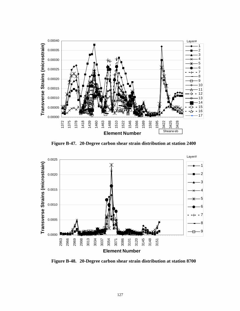
127
0.00000
0.00005
0.00010
0.00015
0.00020
0.00025
0.00030
0.00035
0.00040
1372
1375
1378
1418
1439
1460
1463
1488
1510
1522
1546
1566
1589
1592
1595
3422
3425
3428
Element Number
Tran
sver
se S
trai
ns (m
icro
stra
in) 1
234567891011121314151617
Shearw eb
Layer#
Figure B-47. 20-Degree carbon shear strain distribution at station 2400
0.0000
0.0005
0.0010
0.0015
0.0020
0.0025
2963
2966
2969
2998
3013
3034
3037
3054
3071
3086
3101
3120
3145
3148
3151
Element Number
Tran
sver
se S
trai
ns (m
icro
stra
in)
1
2
3
4
5
6
7
8
9
Layer#
Figure B-48. 20-Degree carbon shear strain distribution at station 8700