Embed Size (px)
Citation preview
U.S.N.A. ---Trident Scholar project report; no. 316 (2003)
Design Specifications Development for Unmanned Aircraft Carrier Landings: A Simulation Approach
by
Midshipman Joseph F. Sweger, Class of 2003 United States Naval Academy
Annapolis, Maryland
_________________________________________ (signature)
Certification of Advisers Approval
CAPT Robert Niewoehner USN
Department of Aerospace Engineering
___________________________________________ (signature)
_________________________
(date)
Acceptance for the Trident Scholar Committee
Professor Joyce E. Shade Deputy Director of Research & Scholarship
___________________________________________
(signature)
_________________________ (date)
Report Documentation Page Form ApprovedOMB No. 0704-0188
Public reporting burden for the collection of information is estimated to average 1 hour per response, including the time for reviewing instructions, searching existing data sources, gathering andmaintaining the data needed, and completing and reviewing the collection of information. Send comments regarding this burden estimate or any other aspect of this collection of information,including suggestions for reducing this burden, to Washington Headquarters Services, Directorate for Information Operations and Reports, 1215 Jefferson Davis Highway, Suite 1204, ArlingtonVA 22202-4302. Respondents should be aware that notwithstanding any other provision of law, no person shall be subject to a penalty for failing to comply with a collection of information if itdoes not display a currently valid OMB control number.
1. REPORT DATE 02 MAY 2003
2. REPORT TYPE N/A
3. DATES COVERED -
4. TITLE AND SUBTITLE Design Specifications Development for Unmanned Aircraft CarrierLandings: A Simulation Approach
5a. CONTRACT NUMBER
5b. GRANT NUMBER
5c. PROGRAM ELEMENT NUMBER
6. AUTHOR(S) 5d. PROJECT NUMBER
5e. TASK NUMBER
5f. WORK UNIT NUMBER
7. PERFORMING ORGANIZATION NAME(S) AND ADDRESS(ES) United States Naval Academy Annapolis, Maryland 21402
8. PERFORMING ORGANIZATIONREPORT NUMBER
9. SPONSORING/MONITORING AGENCY NAME(S) AND ADDRESS(ES) 10. SPONSOR/MONITOR’S ACRONYM(S)
11. SPONSOR/MONITOR’S REPORT NUMBER(S)
12. DISTRIBUTION/AVAILABILITY STATEMENT Approved for public release, distribution unlimited
13. SUPPLEMENTARY NOTES The original document contains color images.
14. ABSTRACT
15. SUBJECT TERMS
16. SECURITY CLASSIFICATION OF: 17. LIMITATION OF ABSTRACT
UU
18. NUMBEROF PAGES
72
19a. NAME OFRESPONSIBLE PERSON
a. REPORT unclassified
b. ABSTRACT unclassified
c. THIS PAGE unclassified
Standard Form 298 (Rev. 8-98) Prescribed by ANSI Std Z39-18
1
ABSTRACT
This project investigated the demands landing precision place upon the physical
configurations of carrier-based unmanned aircraft. The goal was the determination of a
minimum set of performance and maneuverability criteria that ensure satisfactory carrier landing
precision and consistency. The first step was to design and write a comprehensive computer
model to simulate unmanned carrier landings. The model included ship dynamics, atmospheric
turbulence, navigational inaccuracies, dynamic airplane control structure, and aircraft dynamics.
The airplane sensed and corrected for three disturbances: wind gusts, unsteady ship motion, and
navigational information errors. The second step involved varying aircraft attributes and
recording landing performance statistics for each configuration. The influence of each attribute
was extracted from the landing statistics. This was done for various weather conditions because
the ship motion increases with wave size and the gust intensity increases with average wind
velocity. The third step was the development of preliminary design criteria to be refined and
verified with test cases. The fourth and final step was to generate the final aircraft design limits.
The longitudinal design limit is a lift curve slope of at least 2.9 per radian. No bound on
instability or drag was indicated.
Keywords: UAV, UCAV, Automated Landing, Carrier-based
2
ACKNOWLEDGMENTS
First, I would like to thank my advisor, CAPT Niewoehner, for his constant help and
guidance. I certainly could not have done this without him. I would like to thank the JPALS
team at Patuxent River. They were kind enough to share test data for a JPALS error model. Eric
Schug was very helpful. He showed me how to use the data and helped me with all the
necessary coordinate transforms and conversions. Professor Pierce was invaluable in helping to
analyze the Fourier transform of the error signal. He also introduced and showed me how to use
additional tools to look at the time variant frequency content of the signal. LCDR Hallberg also
played a vital role, devising a successful control structure after this project had suffered months
of dead ends. The Trident Committee members provided guidance and gave me this incredible
opportunity. I would also like to thank all of my instructors who have prepared me for this over
the last several years. I could not have done any of this alone.
3
Preface
Unmanned systems are becoming increasingly important to our military. The Chief of
Naval Operations (CNO), Admiral Clark, has stated that advancing technology will have a vital
role in the future of the navy in “Sea Power 21”1. Recent operations in Afghanistan and Iraq
showed that this means unmanned systems, particularly unmanned air vehicles (UAV).
Automated landings are not new. The Automatic Carrier Landing System (ACLS) has
been in use for years, but it was not flight critical because the pilot provided for reversion to
manual control. Consequently, airplanes had been designed for good piloted handling qualities;
if he could handle the airplane, the automatic control system had no difficulty doing the same.
Going to a fully autonomous system permits greater design freedom, no longer constrained by
the limitations of the human operator. The question is how much? This research is intended to
begin to answer that question by defining the design constraints imposed by fully autonomous
carrier landings. This then is a prerequisite technology to the implementation of the CNO's
vision.
1 Clark, V. “Sea Power 21”.
4
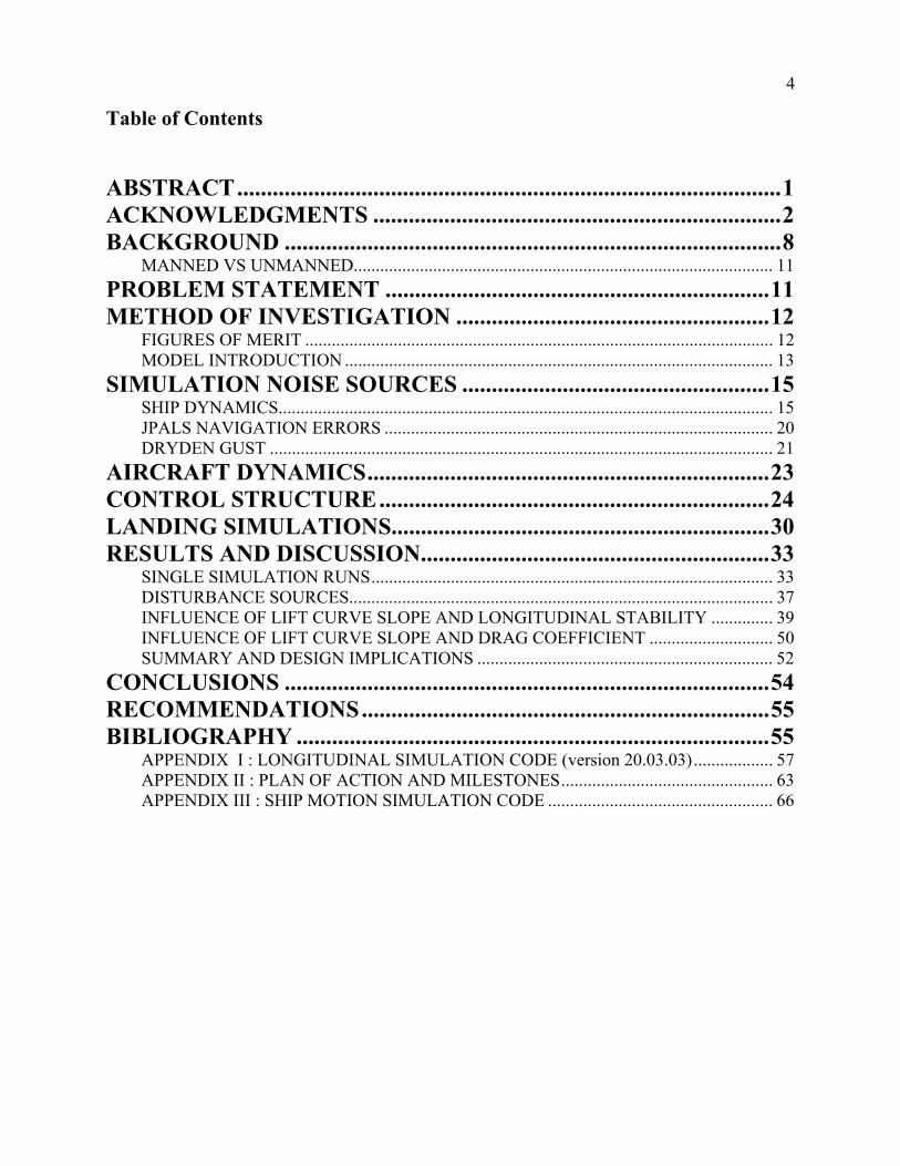
Table of Contents
ABSTRACT............................................................................................1 ACKNOWLEDGMENTS .....................................................................2 BACKGROUND ....................................................................................8
MANNED VS UNMANNED............................................................................................... 11 PROBLEM STATEMENT .................................................................11 METHOD OF INVESTIGATION .....................................................12
FIGURES OF MERIT .......................................................................................................... 12 MODEL INTRODUCTION ................................................................................................. 13
SIMULATION NOISE SOURCES ....................................................15 SHIP DYNAMICS................................................................................................................ 15 JPALS NAVIGATION ERRORS ........................................................................................ 20 DRYDEN GUST .................................................................................................................. 21
AIRCRAFT DYNAMICS....................................................................23 CONTROL STRUCTURE..................................................................24 LANDING SIMULATIONS................................................................30 RESULTS AND DISCUSSION...........................................................33
SINGLE SIMULATION RUNS........................................................................................... 33 DISTURBANCE SOURCES................................................................................................ 37 INFLUENCE OF LIFT CURVE SLOPE AND LONGITUDINAL STABILITY .............. 39 INFLUENCE OF LIFT CURVE SLOPE AND DRAG COEFFICIENT ............................ 50 SUMMARY AND DESIGN IMPLICATIONS ................................................................... 52
CONCLUSIONS ..................................................................................54 RECOMMENDATIONS.....................................................................55 BIBLIOGRAPHY ................................................................................55
APPENDIX I : LONGITUDINAL SIMULATION CODE (version 20.03.03).................. 57 APPENDIX II : PLAN OF ACTION AND MILESTONES................................................ 63 APPENDIX III : SHIP MOTION SIMULATION CODE ................................................... 66
5
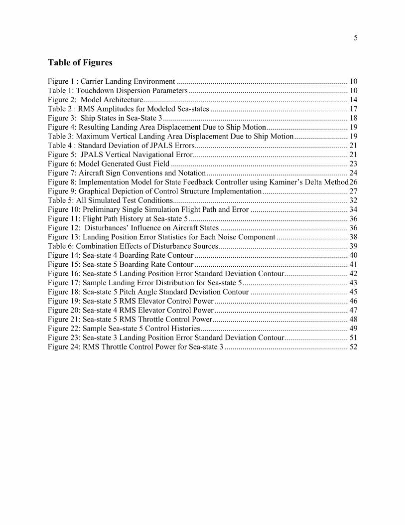
Table of Figures Figure 1 : Carrier Landing Environment ...................................................................................... 10 Table 1: Touchdown Dispersion Parameters ................................................................................ 10 Figure 2: Model Architecture....................................................................................................... 14 Table 2 : RMS Amplitudes for Modeled Sea-states ..................................................................... 17 Figure 3: Ship States in Sea-State 3............................................................................................. 18 Figure 4: Resulting Landing Area Displacement Due to Ship Motion......................................... 19 Table 3: Maximum Vertical Landing Area Displacement Due to Ship Motion........................... 19 Table 4 : Standard Deviation of JPALS Errors............................................................................. 21 Figure 5: JPALS Vertical Navigational Error.............................................................................. 21 Figure 6: Model Generated Gust Field ......................................................................................... 23 Figure 7: Aircraft Sign Conventions and Notation ....................................................................... 24 Figure 8: Implementation Model for State Feedback Controller using Kaminer’s Delta Method26 Figure 9: Graphical Depiction of Control Structure Implementation........................................... 27 Table 5: All Simulated Test Conditions........................................................................................ 32 Figure 10: Preliminary Single Simulation Flight Path and Error ................................................. 34 Figure 11: Flight Path History at Sea-state 5 ................................................................................ 36 Figure 12: Disturbances’ Influence on Aircraft States ................................................................ 36 Figure 13: Landing Position Error Statistics for Each Noise Component .................................... 38 Table 6: Combination Effects of Disturbance Sources................................................................. 39 Figure 14: Sea-state 4 Boarding Rate Contour ............................................................................. 40 Figure 15: Sea-state 5 Boarding Rate Contour ............................................................................. 41 Figure 16: Sea-state 5 Landing Position Error Standard Deviation Contour................................ 42 Figure 17: Sample Landing Error Distribution for Sea-state 5..................................................... 43 Figure 18: Sea-state 5 Pitch Angle Standard Deviation Contour ................................................. 45 Figure 19: Sea-state 5 RMS Elevator Control Power ................................................................... 46 Figure 20: Sea-state 4 RMS Elevator Control Power ................................................................... 47 Figure 21: Sea-state 5 RMS Throttle Control Power.................................................................... 48 Figure 22: Sample Sea-state 5 Control Histories.......................................................................... 49 Figure 23: Sea-state 3 Landing Position Error Standard Deviation Contour................................ 51 Figure 24: RMS Throttle Control Power for Sea-state 3 .............................................................. 52
6
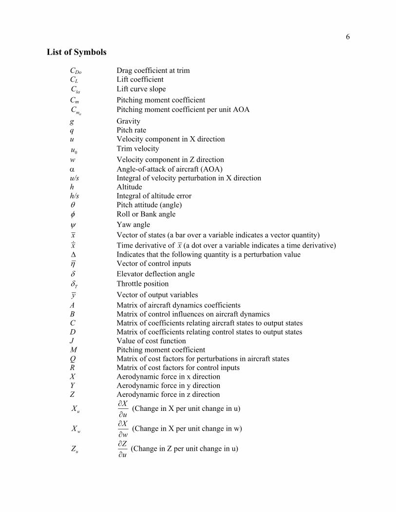
List of Symbols
CDo Drag coefficient at trim CL Lift coefficient
lC α Lift curve slope Cm Pitching moment coefficient
mCα
Pitching moment coefficient per unit AOA g Gravity q Pitch rate u Velocity component in X direction
0u Trim velocity w Velocity component in Z direction α Angle-of-attack of aircraft (AOA) u/s Integral of velocity perturbation in X direction h Altitude h/s Integral of altitude error θ Pitch attitude (angle) φ Roll or Bank angle ψ Yaw angle x Vector of states (a bar over a variable indicates a vector quantity) x& Time derivative of x (a dot over a variable indicates a time derivative) ∆ Indicates that the following quantity is a perturbation value η Vector of control inputs δ Elevator deflection angle
Tδ Throttle position y Vector of output variables A Matrix of aircraft dynamics coefficients B Matrix of control influences on aircraft dynamics C Matrix of coefficients relating aircraft states to output states D Matrix of coefficients relating control states to output states J Value of cost function M Pitching moment coefficient
Q Matrix of cost factors for perturbations in aircraft states R Matrix of cost factors for control inputs X Aerodynamic force in x direction Y Aerodynamic force in y direction Z Aerodynamic force in z direction
uX Xu
∂∂
(Change in X per unit change in u)
wX Xw∂∂
(Change in X per unit change in w)
uZ Zu∂∂
(Change in Z per unit change in u)
7
wZ Zw∂∂
(Change in Z per unit change in w)
uM Mu
∂∂
(Change in M per unit change in u)
wM Mw
∂∂
(Change in M per unit change in w)
qM Mq
∂∂
(Change in M per unit change in q)
Xδ Xδ∂∂
(Change in X per unit change in elevator deflection)
Zδ Zδ∂∂
(Change in Z per unit change in elevator deflection)
Mδ Mδ
∂∂
(Change in M per unit change in elevator deflection)
TXδ T
Xδ∂∂
(Change in X per unit change in throttle)
TZδ T
Zδ∂∂
(Change in Z per unit change in throttle)
TMδ T
Mδ∂∂
(Change in M per unit change in throttle)
8
BACKGROUND
Carrier landings define naval aviation. These landing requirements drive the design of both
the aircraft and the ship, with the landing airspeed constituting one of the most significant
attributes of the problem. The correct determination of the approach speed is vital. It is the
balance of landing safely and causing unnecessary wear, which results in higher maintenance
requirements and shorter service life. Higher landing speeds decrease the maximum landing
weight. This means an aircraft must land with less ordnance and fuel. The determination of the
approach speed for manned aircraft is the minimum speed that simultaneously satisfies several
criteria. These criteria can be found in diverse military specifications and include the following2:
a. Aerodynamic stall margin of 10%
b. Field of view (over the nose visibility)
c. Flight qualities (defined in MIL-STD-8785/1797)
d. Compatibility with Wind Over the Deck (WOD)
e. Longitudinal Acceleration in level flight of 5 ft/sec2 within 2.5 seconds in full power
f. Pop-up, 50 ft. glide slope transfer with stick only in 5 seconds
g. Minimum single engine rate of climb: 500 ft/min (tropical day)
The goal of landing speed criteria is to facilitate the design of aircraft that can consistently
make safe carrier landings. These historic requirements were recently reviewed for manned
aircraft. While Navy contractors have performed simulation trials of aircraft under design, no
criteria exist for unmanned aircraft distinct from manned. No study has been done to determine
2 Rudowski et al, Review of Carrier Approach Criteria for Carrier-based Aircraft p.22
9
the range of aircraft attributes necessary for an unmanned aircraft to land safely. The referenced
Heffley report attempted to perform this evaluation for the case of manned aircraft3.
Understanding the carrier-landing task requires some discussion of terminology. Angle
of attack (AOA) is the angle between where the airplane is pointed and where it is going. This
value along with the velocity determines the amount of lift generated. An aircraft’s pitch angle
is where the nose is pointed relative to the horizon and for manned aircraft strongly influences
the over the nose visibility from the cockpit. Sink rate is the vertical component of the velocity.
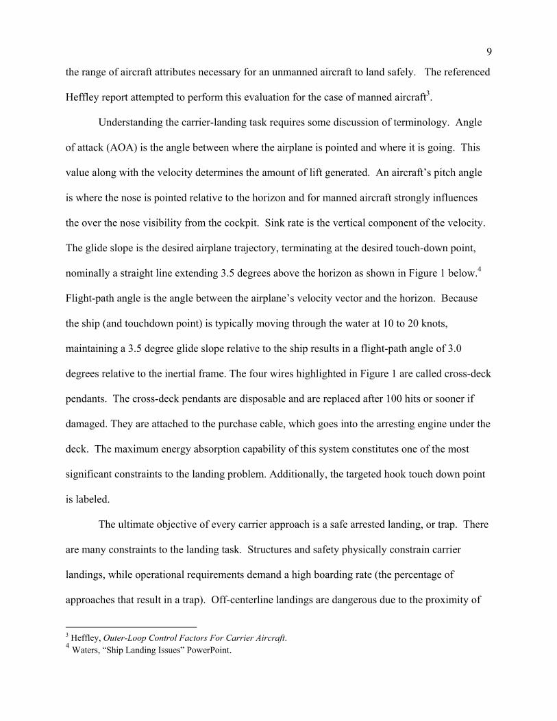
The glide slope is the desired airplane trajectory, terminating at the desired touch-down point,
nominally a straight line extending 3.5 degrees above the horizon as shown in Figure 1 below.4
Flight-path angle is the angle between the airplane’s velocity vector and the horizon. Because
the ship (and touchdown point) is typically moving through the water at 10 to 20 knots,
maintaining a 3.5 degree glide slope relative to the ship results in a flight-path angle of 3.0
degrees relative to the inertial frame. The four wires highlighted in Figure 1 are called cross-deck
pendants. The cross-deck pendants are disposable and are replaced after 100 hits or sooner if
damaged. They are attached to the purchase cable, which goes into the arresting engine under the
deck. The maximum energy absorption capability of this system constitutes one of the most
significant constraints to the landing problem. Additionally, the targeted hook touch down point
is labeled.
The ultimate objective of every carrier approach is a safe arrested landing, or trap. There
are many constraints to the landing task. Structures and safety physically constrain carrier
landings, while operational requirements demand a high boarding rate (the percentage of
approaches that result in a trap). Off-centerline landings are dangerous due to the proximity of
3 Heffley, Outer-Loop Control Factors For Carrier Aircraft. 4 Waters, “Ship Landing Issues” PowerPoint.
10
personnel and equipment; short (low) approaches hazard striking the aft end of the ship. High
approaches will fail to catch a wire. The structural limits of the hook and cross-deck pendant
determine the maximum landing velocity. Sink rate is limited by the landing gear structure.
Additionally, hook geometry requires the aircraft to land with a positive pitch angle, optimally
five degrees, because the main gear must touchdown first. The positive pitch angle is also
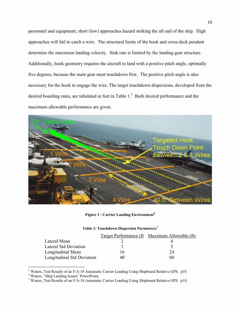
necessary for the hook to engage the wire. The target touchdown dispersions, developed from the
desired boarding rates, are tabulated in feet in Table 1.5 Both desired performance and the
maximum allowable performance are given.
Figure 1 : Carrier Landing Environment6
Table 1: Touchdown Dispersion Parameters7
Target Performance (ft Maximum Allowable (ft)Lateral Mean 2 4 Lateral Std Deviation 3 5 Longitudinal Mean 16 24 Longitudinal Std Deviation 40 60
5 Waters, Test Results of an F/A-18 Automatic Carrier Landing Using Shipboard Relative GPS. p10. 6 Waters, “Ship Landing Issues” PowerPoint. 7 Waters, Test Results of an F/A-18 Automatic Carrier Landing Using Shipboard Relative GPS. p10.
11
MANNED VS UNMANNED
Historically, designing an airplane for the carrier-landing task has been constrained by
the limitations of the pilot as an integral part of the control system. The full capabilities of
automated control systems have never previously been explored. The human operator has
difficulty tracking multiple parameters at once. Part of the difficulty is focusing one’s vision on
the ship for line-up and glide slope then back to instruments in the cockpit to read airspeed and
angle of attack. People also lack the precision and reaction time of computers. Consequently, if
an airplane’s handling qualities satisfied a human pilot, the legacy automated systems (e.g. SPN-
42 Automatic Carrier Landing System (ACLS)) could easily handle the airplane. Moreover,
ACLS was neither flight critical nor attempted at severe sea-states. The move to unmanned
systems permits design liberties fully capitalizing on the capabilities of an automated system, yet
raises the automated system to the status of “flight critical”. If the control system cannot
successfully get the vehicle aboard, it is lost at sea.
PROBLEM STATEMENT
The above pre-requisite background now permits a concise statement of this study’s aim.
Given the disturbance environment characterized by realistic atmospheric turbulence,
navigational inaccuracies, ship motion, the required performance metrics, and a specified
controls strategy, define the major aerodynamic performance and controllability limitations upon
the design of an autonomous carrier-based airplane. The problem is not, “given an airplane, find
a control system that satisfies the performance requirements.” Instead the goal is to define the
12
range of airplane attributes which, in concert with an automatic control system, can satisfy the
Table 1 performance requirements.
METHOD OF INVESTIGATION
A Monte Carlo simulation approach was used. A sensitivity analysis of the influence of
several characteristics of the airplane on the landing performance was conducted in the presence
of representative disturbances, including navigation errors, gusts, and ship motion. These results
were used to define the range of suitable airplane characteristics. This methodology is broken
down into small pieces and given as a tabular timeline in Appendix II.
FIGURES OF MERIT
Operationally, boarding rate and safety are the primary concerns. From these, several
other performance targets have been derived, such as landing dispersion and pitch attitude
variation, which are easier for the engineers to use and tend to force designs to meet the
operational needs. Landings from eighty feet short to sixty feet long would all achieve a
successful arrestment, based solely on the placement of the four cross-deck pendants. This
measurement, along with the desired boarding rate provided the origin of the landing dispersion
requirements listed previously in Table 1.
The pitch attitude constraints come from several sources. The nose must be pitched up to
avoid landing nose gear first and to reduce approach speed it is desirable to fly near stall speed.
Excessive nose up pitch is unacceptable because of stall concerns and the hook is prone to skip
over the wires. Large variations in pitch mean large variations in AOA as well. This is
undesirable because it forces an increased stall margin and therefore an increased approach speed
and lower allowable landing weight.
13
Finally, the total control power available from the control surfaces constitutes a major
configuration feature of an airplane, particular at low speeds where the low dynamics pressure
yields poor sensitivity (expressed in torque about the airplane center of gravity per degree of
control deflection). For greater control power (which we’ll express in root-mean-square (RMS)
activity), faster or more powerful control actuators increase the weight and cost of those systems.
This makes a high control power requirement undesirable.
MODEL INTRODUCTION
The simulation models consisted of multiple systems of differential equations. For
example, the full six-degrees-of-freedom (6-DoF) aircraft dynamics model consists of twelve,
first-order non-linear coupled differential equations. Due to time constraints, this study restricted
itself to an investigation of the longitudinal behavior of the airplane (3-DoF). In this case,
MATLAB was used to solve a discrete-time difference equation, numerically converted from six
linear differential equations (two additional integrated states will appear later in the controller in
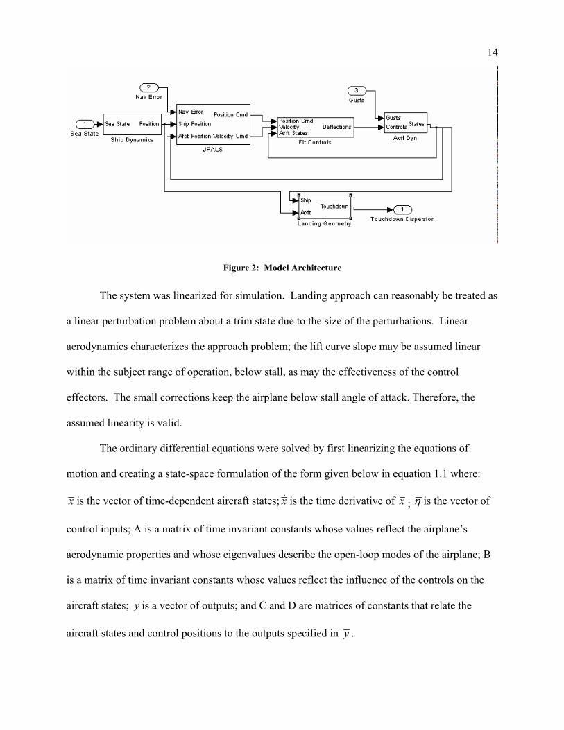
order to provide integral action). Figure 2, the flow chart below, depicts a visualization of the
unmanned carrier landing simulation system. The three sources of noise injected into the
simulation are numbered circles. Although not shown here, each box contains another diagram
depicting the interactions of the governing equations for that aspect of the system. The arrows
show the flow of information from one sub-system to the next. Each simulation run terminated
with the collection of a touchdown point and orientation. The MATLAB simulation code is
attached as Appendix I. Comments are included in the code describing the function of parts of
the code as well as limited explanations for what has been included and what has been neglected.
14
Figure 2: Model Architecture
The system was linearized for simulation. Landing approach can reasonably be treated as
a linear perturbation problem about a trim state due to the size of the perturbations. Linear
aerodynamics characterizes the approach problem; the lift curve slope may be assumed linear
within the subject range of operation, below stall, as may the effectiveness of the control
effectors. The small corrections keep the airplane below stall angle of attack. Therefore, the
assumed linearity is valid.
The ordinary differential equations were solved by first linearizing the equations of
motion and creating a state-space formulation of the form given below in equation 1.1 where:
x is the vector of time-dependent aircraft states; x& is the time derivative of x ; η is the vector of
control inputs; A is a matrix of time invariant constants whose values reflect the airplane’s
aerodynamic properties and whose eigenvalues describe the open-loop modes of the airplane; B
is a matrix of time invariant constants whose values reflect the influence of the controls on the
aircraft states; y is a vector of outputs; and C and D are matrices of constants that relate the
aircraft states and control positions to the outputs specified in y .
15
x Ax By Cx D
ηη
= += +
& (1.1)
This type of system is described as linear time invariant, LTI, because the governing
differential equations are linear and the coefficients are not time dependent. This continuous-
time system was then converted by functions in the MATLAB Control Toolbox to a discrete
time state-space formulation, which is solved numerically by constant-time-step difference
equations of the form shown below where the subscripted ‘d’ indicates a discrete time matrix.
( 1) ( ) (( 1) ( ) (
d d
d d
))
x k A x k By k C x k D k
kηη
+ = ++ = +
(1.2)
A ten-millisecond time step (0.01 sec) was selected to match the ship motion model
(discussed below) provided by the Naval Air Systems Command (NAVAIR). This interval was
more than fast enough to accurately model the aircraft dynamics linearly, with the sample rate
over 100 times that of the fastest airplane dynamic mode. The time step was consequently much
smaller than necessary, but the speed of the computational capability permitted this
extravagance.
SIMULATION NOISE SOURCES
SHIP DYNAMICS
At the suggestion of engineers from NAVAIR, the dynamics and dimensions of CVN 65,
the U.S.S. Enterprise, were employed throughout the study. The distances from the ship’s center
of motion to the landing area in feet are 223 aft, 64 up, and 10 left.
16
The ship dynamics model provided by NAVAIR generated six degree-of-freedom time
histories of ship motion for a sea-state chosen by the user. The provided ship dynamics code is
included in Appendix III. Ship pitch is positive nose up, roll is positive to the left, and yaw is
positive nose left. Note that all ship displacements are referenced to the ship center of motion.
Since the desired touch down point was displaced a significant vertical and horizontal distance
from the center of motion, the touchdown point's translational displacement was dependent upon
both the translational and angular displacements of the ship. These angles had to be converted to
distances in X, Y, and Z to be useful to the landing task. Equations 1.3 through 1.5 given below
are the exact relationships.
(1.3) ch pitch pitch roll rollZ = -223*sin(S ) + 64*cos(S )*cos(S ) -64 -10*sin(S )
(1.4) ch roll pitch yaw yawY = 64*sin(S ) +10*cos(S )*cos(S ) -10 +223*sin(S )
(1.5) ch pitch yaw pitch yawX = 223*cos(S )*cos(S ) -223 +64*sin(S ) -10*sin(S )
The system linearizes under a small angle assumption. At sea-state 5, the most severe
conditions modeled, the RMS value for the ship’s pitch was only 1.83 degrees, well within the
small angle criterion. Under the small angle approximation, cosine terms go to unity and sine
terms reduce to the angle expressed in radians. The resulting system is shown below as
equations 1.6 through 1.8.
(1.6) ch pitch rollZ = -223*S -10*S
(1.7) ch roll yawY = 64*S +223S
(1.8) ch pitch yawX = 64*S -10*S
17
This system may be used to model the complete ship-aircraft system. Again, for the
purposes of this report, only longitudinal dynamics were modeled. The effects of ship pitch
alone are given in equations 1.9 and 1.10.
(1.9) ch pitchZ = -223*S
(1.10) ch pitchX = 64*S
“Surge”, “heave”, and “sway” describe linear translations of the ship about its center of
motion fore or aft, up or down, and sideways respectively. These displacements were added
directly to the translational displacement. Thus, the vertical and horizontal displacements of the
landing area, due to the influence of ship motion are:
(1.11) ch pitchZ = -223*S +heave
(1.12) ch pitchX = 64*S +surge
For the purposes of this study, sea-states 3, 4, and 5 were modeled. Table 2 provides the
relevant RMS amplitudes.
Table 2 : RMS Amplitudes for Modeled Sea-states
Sea-state Heave (ft) Surge (ft) Pitch (deg)
3 2.11 0.838 0.763
4 3.81 1.4 1.22
5 5.06 2.1 1.83
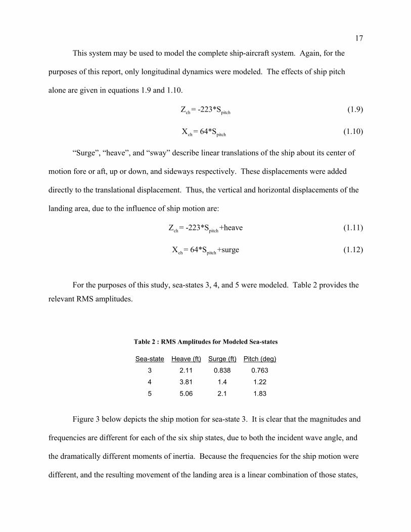
Figure 3 below depicts the ship motion for sea-state 3. It is clear that the magnitudes and
frequencies are different for each of the six ship states, due to both the incident wave angle, and
the dramatically different moments of inertia. Because the frequencies for the ship motion were
different, and the resulting movement of the landing area is a linear combination of those states,
18
a distinct “beating” pattern is observed. As the phase of the ship motion influenced the landing
precision of the aircraft, care was taken to distribute the simulation initial conditions across the
full spectrum of ship states. For the longitudinal problem, only half of these states have
significant influence as shown in equations 1.11 and 1.12. The other three states are neglected
for simplicity. The magnitudes in Figure 3 below show that the surge is less than half the
magnitude of the heave. The surge must be scaled by the glide slope, or multiplied by 0.06, to
arrive at the change in commanded altitude. Consequently, although surge is included in the
model, its effect on the commanded altitude is only 3% of the influence of heave.
Figure 3: Ship States in Sea-State 3
For the longitudinal problem, pitch, heave, and surge influence the height of the target
landing area about its mean position. The total influence of ship motion for all three modeled
&
'1
1
Q
-\
4
2
^ -2
-4
002
QGI
0
-□01
■0 02
Shi[i Molicin in Se*Sl3le 3
□.S 1 ^ 5 2
06 I 16 2 dislancB (H) ^ ,|-|l
0.6 1 16 2
^ 0.5
Q
4J.6
-1
□-□1
0 006
□ -0 006
-□□I
□ 05 1 15 2
0
r -2
06 1 dislancE (H)
1 6
' 10
0 06 1 16 2 diglance (ft) -Q''
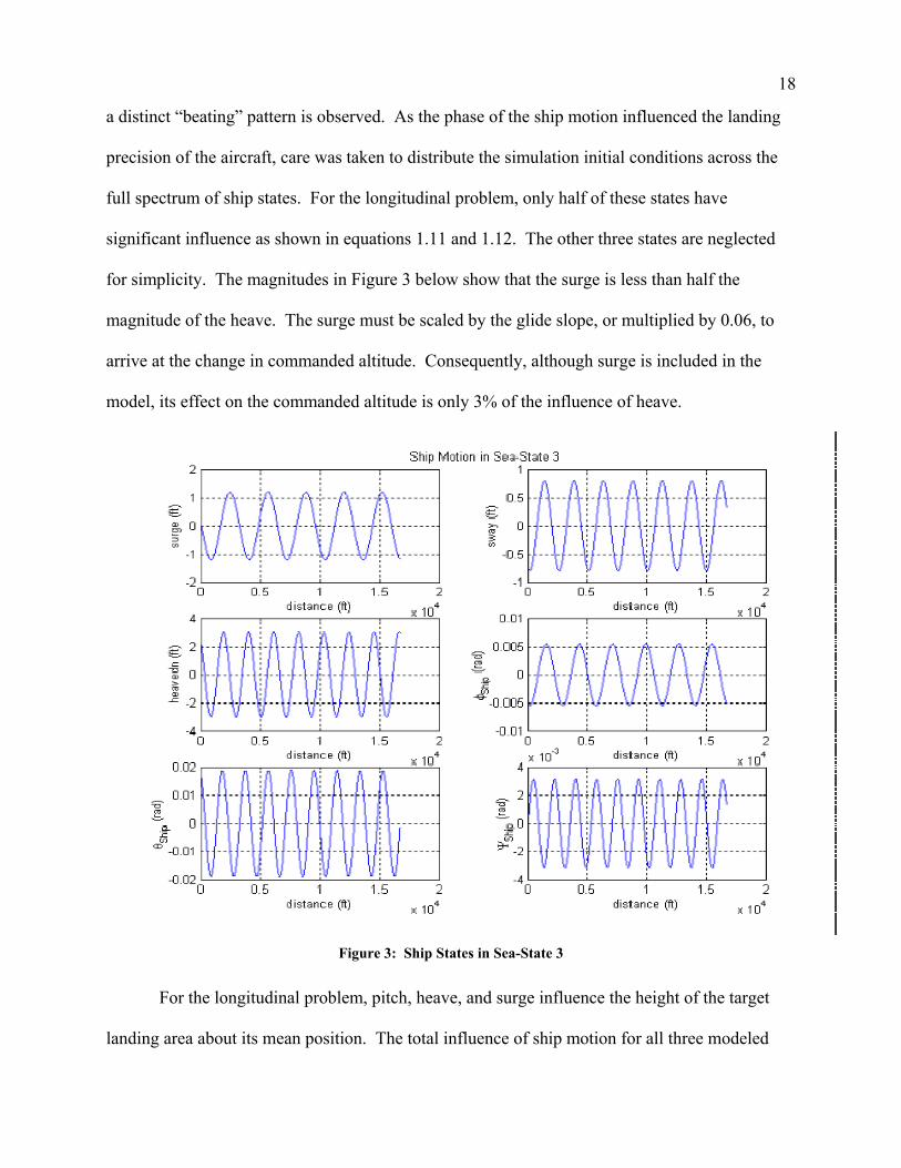
19
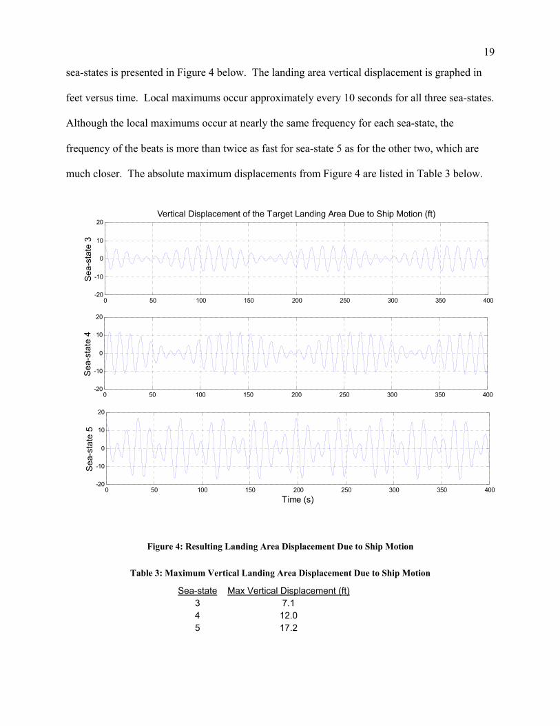
sea-states is presented in Figure 4 below. The landing area vertical displacement is graphed in
feet versus time. Local maximums occur approximately every 10 seconds for all three sea-states.
Although the local maximums occur at nearly the same frequency for each sea-state, the
frequency of the beats is more than twice as fast for sea-state 5 as for the other two, which are
much closer. The absolute maximum displacements from Figure 4 are listed in Table 3 below.
0 50 100 150 200 250 300 350 400-20
-10
0
10
20
Sea
-sta
te 3
Vertical Displacement of the Target Landing Area Due to Ship Motion (ft)
0 50 100 150 200 250 300 350 400-20
-10
0
10
20
Sea
-sta
te 4
0 50 100 150 200 250 300 350 400-20
-10
0
10
20
Sea
-sta
te 5
Time (s)
Figure 4: Resulting Landing Area Displacement Due to Ship Motion
Table 3: Maximum Vertical Landing Area Displacement Due to Ship Motion
Sea-state Max Vertical Displacement (ft)3 7.1 4 12.0 5 17.2
20
JPALS NAVIGATION ERRORS
The Joint Precision Automated Landing System (JPALS), currently under development
for use by both the Navy and Air Force, will surely serve as the guidance system on first
generation unmanned shipboard aircraft. JPALS operates using differential-GPS data, blended
with inertial navigation on both the airplane and the carrier. The blended data takes advantage of
the high accuracy of inertial navigation systems over relatively short periods of time, updated by
GPS at a lower frequency, in a process called complementary filtering. Differential GPS
accuracy is achieved without correction factors because the critical value is the position of the
aircraft relative to the ship as opposed to the absolute position of either in the world. The
proximity of the ship and airplane during approach and landing cause both GPS receivers to
experience the same atmospheric errors, resulting in very tight error bounds.
NAVAIR provided one and a half hours of JPALS flight test data sampled at 50 Hz. with
both the measured and the true position. This data provided the basis for the navigation error
injected into the simulation model. The position errors were evaluated as a horizontal and
vertical component. The physical principles behind GPS yield better resolution in the horizontal
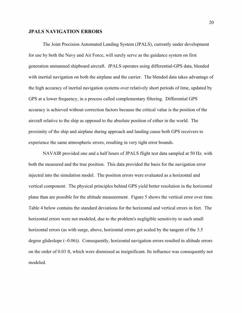
plane than are possible for the altitude measurement. Figure 5 shows the vertical error over time.
Table 4 below contains the standard deviations for the horizontal and vertical errors in feet. The
horizontal errors were not modeled, due to the problem's negligible sensitivity to such small
horizontal errors (as with surge, above, horizontal errors get scaled by the tangent of the 3.5
degree glideslope (~0.06)). Consequently, horizontal navigation errors resulted in altitude errors
on the order of 0.03 ft, which were dismissed as insignificant. Its influence was consequently not
modeled.
21
Table 4 : Standard Deviation of JPALS Errors
JPALS Error Component JPALS Error Component HorizontalHorizontal Vertical Vertical Standard deviation (ft) Standard deviation (ft) 0.2939 0.2939 0.6467 0.6467
JPALS Vertical Navigation Errors 5 4 3
JPA
LS e
rror
(ft)
2 1 0
-1 -2
0-3 1000 5000 2000 3000 4000 6000
Time (s)
Figure 5: JPALS Vertical Navigational Error
Frequency analysis with Fourier series transforms and windowed Fourier transforms was
performed to identify any frequency dependence of the JPALS error signal. No frequency
dependence was noted, indicating superb blending of the GPS and INS data in a complementary
filter. Although there are some transient characteristics in the navigation error, an uncolored
model was deemed sufficient and used for simplicity. Consequently, the modeled navigational
error signal was a normally distributed random number with the standard deviation shown above.
DRYDEN GUST DRYDEN GUST
The Dryden gust model is the industry standard atmospheric turbulence model, as
stipulated by the military flying qualities specification, MIL-STD-8785C. The model utilizes a
The Dryden gust model is the industry standard atmospheric turbulence model, as
stipulated by the military flying qualities specification, MIL-STD-8785C. The model utilizes a
22
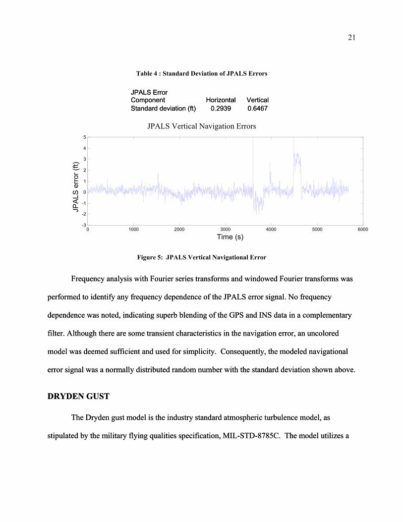
white noise source (a Gaussian distributed random number) filtered by a second-order system.
The matrices below provide the gust filter.8
12g
g
g g Vug L
Vu uL
σ w = − +
& (1.13)
233
2
30 1
2(1 2 3)
g
g
wg
g gw wg g
g gw
g
VLw w
wV Vw w VL LL
σ
σ
= +− − −
&
& (1.14)
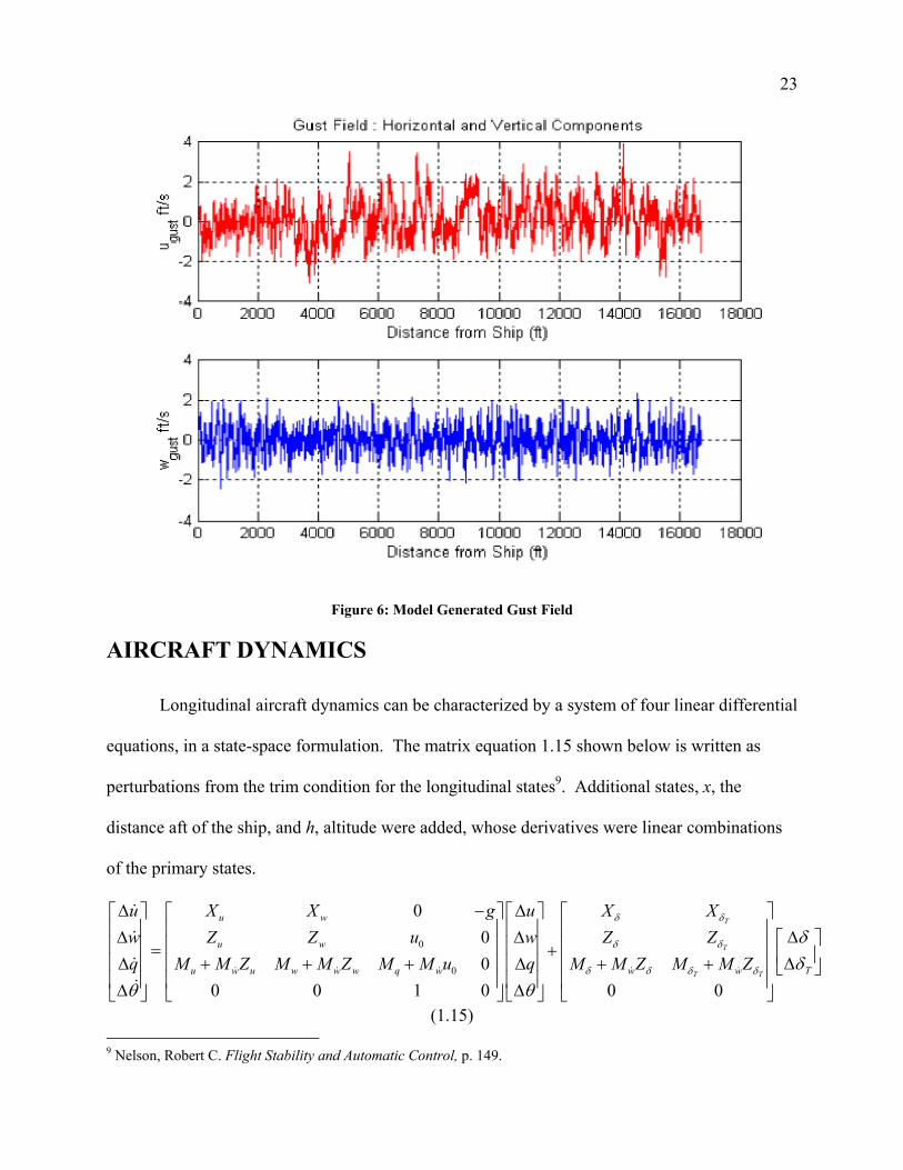
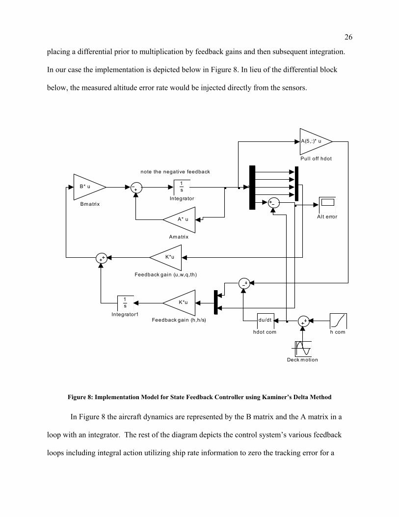
The graph below is a sample turbulence field behind the ship. The gust intensity increases with
altitude then becomes constant. The intensity also increases with the average wind velocity. The
gust field below models a 20-knot average wind speed at an altitude of 50 meters. The gust data
was generated by similarly converting the above continuous time system of equations into
discrete time difference equations, with a ten-millisecond time step, identical to the aircraft
simulation.
8 Mulder and Van der Vaart, "Lecture Notes Dictaat D-47: Aircraft Response to Atmospheric Turbulence," p. 209-10.
23
Figure 6: Model Generated Gust Field
AIRCRAFT DYNAMICS
Longitudinal aircraft dynamics can be characterized by a system of four linear differential
equations, in a state-space formulation. The matrix equation 1.15 shown below is written as
perturbations from the trim condition for the longitudinal states9. Additional states, x, the
distance aft of the ship, and h, altitude were added, whose derivatives were linear combinations
of the primary states.
0
0
000
0 0 1 0 0 0
T
T
T T
u w
u w
Tu w u w w w q w w w
u X X g u X Xw Z Z u w Z Zq M M Z M M Z M M u q M M Z M M Z
δ δ
δ δ
δ δ δ δ
δδ
θ θ
∆ − ∆ ∆∆ ∆ = + ∆∆ + + + ∆ + + ∆ ∆
& & & & &
&
&
&&
(1.15) 9 Nelson, Robert C. Flight Stability and Automatic Control, p. 149.
4
2
-2
-■1
2
-2
-4
Gust Pield : Horizontal and Veitical OomponentG
0 2000 4000 6000 8000 10000 12000 14000 16000 18000 DJslance from Ship 01)
D 2000 4000 6000 BOOO 10000 12000 14000 16000 ISOOO Distance from Ship (II)
24
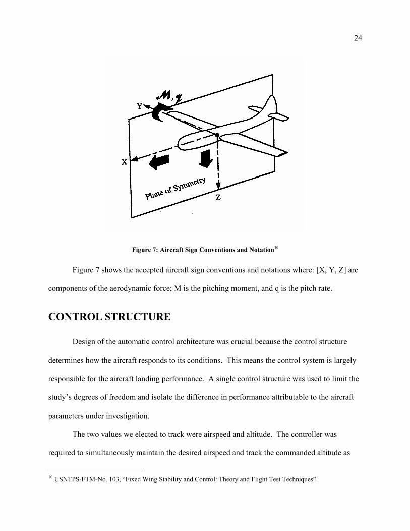
Figure 7: Aircraft Sign Conventions and Notation10
Figure 7 shows the accepted aircraft sign conventions and notations where: [X, Y, Z] are
components of the aerodynamic force; M is the pitching moment, and q is the pitch rate.
CONTROL STRUCTURE
Design of the automatic control architecture was crucial because the control structure
determines how the aircraft responds to its conditions. This means the control system is largely
responsible for the aircraft landing performance. A single control structure was used to limit the
study’s degrees of freedom and isolate the difference in performance attributable to the aircraft
parameters under investigation.
The two values we elected to track were airspeed and altitude. The controller was
required to simultaneously maintain the desired airspeed and track the commanded altitude as
10 USNTPS-FTM-No. 103, “Fixed Wing Stability and Control: Theory and Flight Test Techniques”.
25
precisely as possible. Airspeed regulation was important for the structural and aerodynamic
implications cited above. Precise altitude control was necessary to meet the landing touchdown
dispersion requirement. To accomplish these, integral tracking on airspeed was required to
maintain approach speed and AOA (regulating one has the effect of regulating both, due to their
mathematical relationship). Integral tracking was also required on altitude to track the glide
slope, which the controller viewed as a ramp input (With altitude as a state, the system was
Type-1. The additional integrator was required to achieve zero steady-state error in response to a
pure ramp input.).
Sensors are also important because any feedback control system depends upon measured
values for its calculation of control deflections. All aircraft states were reasonably assumed
known and available for state feedback from commonly installed production aircraft
instrumentation. The only modeled sensor errors were the JPALS navigation errors.
Development of a suitable control architecture proved to be difficult. Specifically, the
thorny problem was determining a control architecture that would permit the controller to take
advantage of the known ship pitch and heave rates to track a command composed of the
superposition of a ramp and a complex sinusoidal. These values are reasonably known from
ship-based accelerometers and rate gyros, and capable of providing lead compensation to
improve the ability of the airplane to track a pitching, heaving deck. The particular challenge was
implementing lead compensation in a state-space formulation. This was done using the Delta-
implementation model devised by Kaminer.11 Though originally introduced for the purpose of
improving the robustness of gain-scheduled controllers, it also resolved our problem of using the
altitude error rate to provide lead tracking. The Delta-implementation involves conceptually
11 Kaminer, “A Velocity Algorithm for the Implementation of Nonlinear Gain-Scheduled Controllers”, Automatica, Vol. 31, pp. 1185--1191.
26
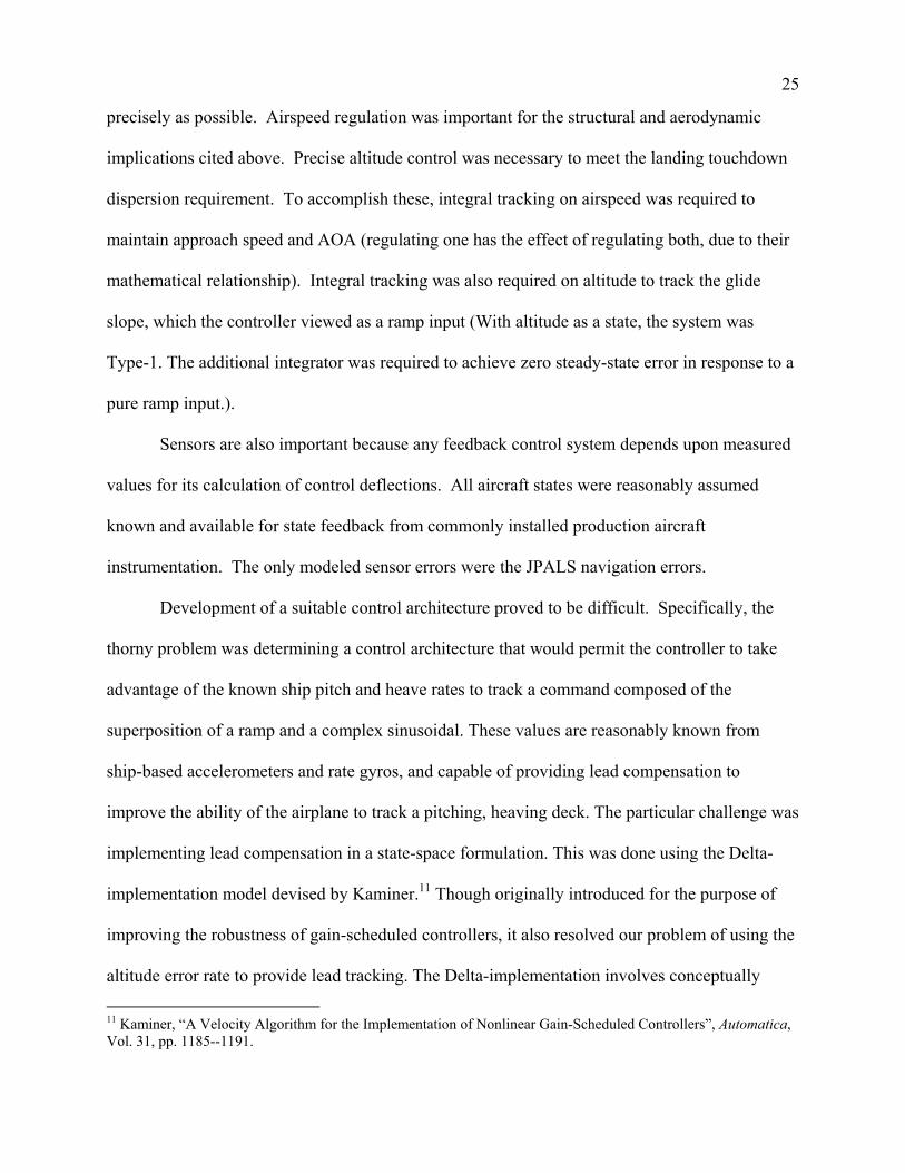
placing a differential prior to multiplication by feedback gains and then subsequent integration.
In our case the implementation is depicted below in Figure 8. In lieu of the differential block
below, the measured altitude error rate would be injected directly from the sensors.
note the negative feedback
du/dt
hdot com h com
A(5,:)* u
Pul l off hdot
1s
Integrator1
1s
Integrator
K*u
Feedback gain (u,w,q,th)
K*u
Feedback gain (h,h/s)
emu
Deck motion
B* u
Bmatrix
A* u
Amatrix
Al t error
Figure 8: Implementation Model for State Feedback Controller using Kaminer’s Delta Method
In Figure 8 the aircraft dynamics are represented by the B matrix and the A matrix in a
loop with an integrator. The rest of the diagram depicts the control system’s various feedback
loops including integral action utilizing ship rate information to zero the tracking error for a
27
ramp input. The derivative feedback provides lead compensation to improve the tracking of the
complex sinusoidal deck motion.
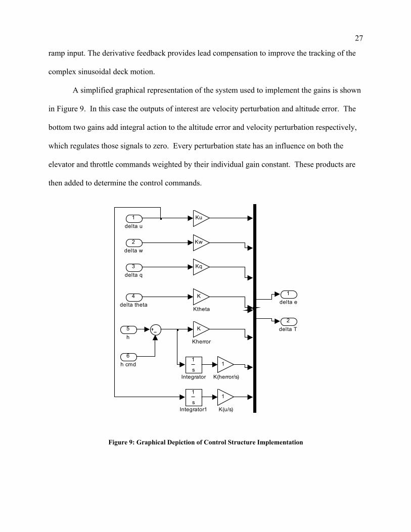
A simplified graphical representation of the system used to implement the gains is shown
in Figure 9. In this case the outputs of interest are velocity perturbation and altitude error. The
bottom two gains add integral action to the altitude error and velocity perturbation respectively,
which regulates those signals to zero. Every perturbation state has an influence on both the
elevator and throttle commands weighted by their individual gain constant. These products are
then added to determine the control commands.
2delta T
1delta e
K
Ktheta
K
Kherror
1
K(u/s)
1
K(herror/s)
s
1
Integrator1
s
1
Integrator
m
Kq
Kw
Ku
6h cmd
5h
4delta theta
3delta q
2delta w
1delta u
Figure 9: Graphical Depiction of Control Structure Implementation
28
Figure 9 depicts the aircraft states being multiplied by their respective gains and summed
for the resulting elevator and throttle commands. These gains were calculated by the ‘lqry’
function in MATLAB, which is a linear quadratic regulator (LQR) with output weighting. The
lqry command calculates state-feedback gains to minimize a cost function, provided as
equation 1.15, for the specified system and weightings; however, the implementation system and
the system for gain calculations are not the same. The difference is the gains are calculated for h
and hs
making it a regulator problem, but the implementation used herror and errorhs
transforming
it to a tracking problem. The matrix weights the output states, and Q R weights the control
inputs.
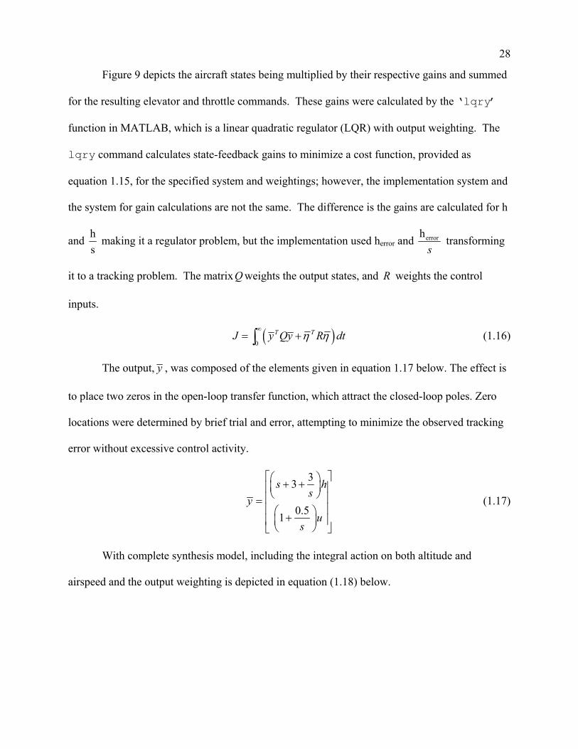
( )0
T TJ y Qy Rη η∞
= +∫ dt (1.16)
The output, y , was composed of the elements given in equation 1.17 below. The effect is
to place two zeros in the open-loop transfer function, which attract the closed-loop poles. Zero
locations were determined by brief trial and error, attempting to minimize the observed tracking
error without excessive control activity.
33
0.51
s hs
yu
s
+ + = +
(1.17)
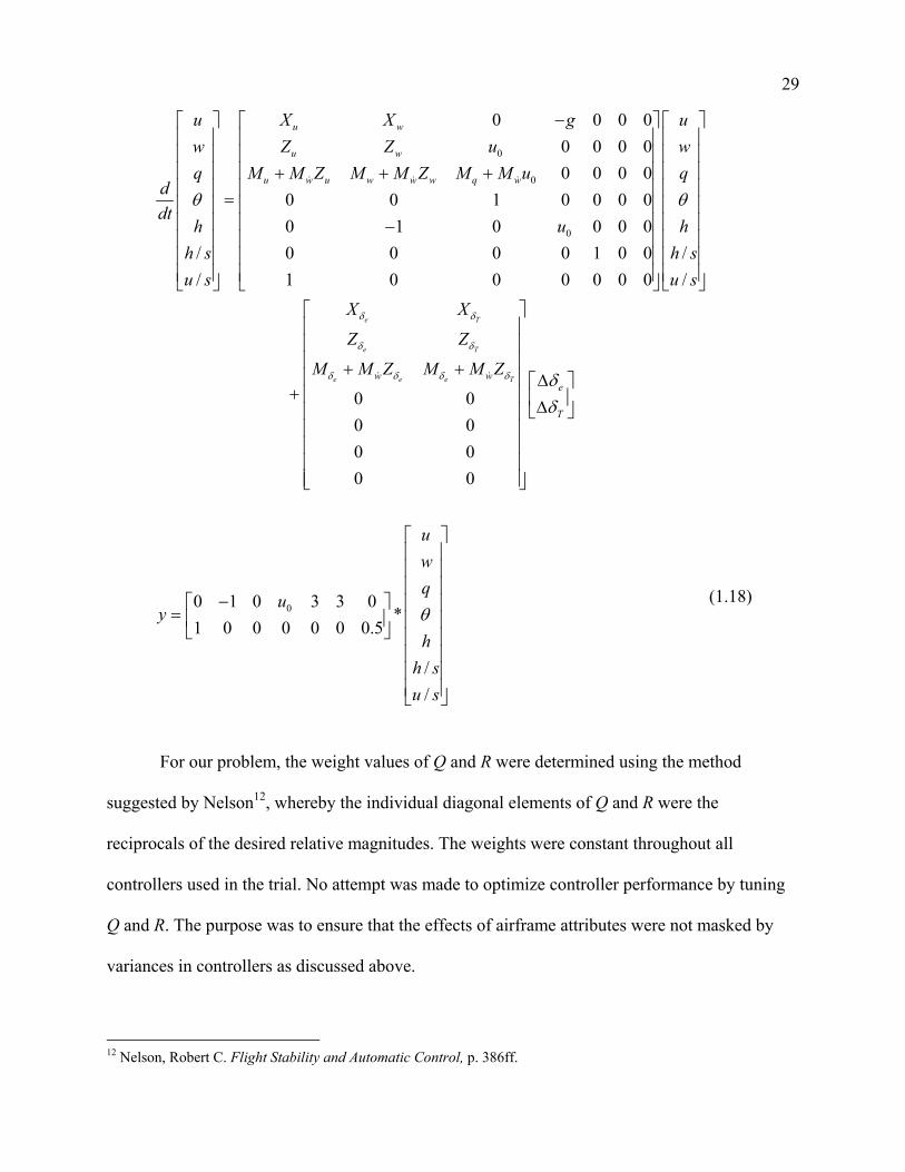
With complete synthesis model, including the integral action on both altitude and
airspeed and the output weighting is depicted in equation (1.18) below.
29
0
0
0
0 0 0 00 0 0 00 0 0 0
0 0 1 0 0 0 00 1 0 0 0 0
/ 0 0 0 0 1 0 0 // 1 0 0 0 0 0 0
e T
e T
e e e
u w
u w
u w u w w w q w
w w
u X X gw Z Z uq M M Z M M Z M M u q
ddt
h uh s h su s u s
X X
Z Z
M M Z M M
δ δ
δ δ
δ δ δ
/
uw
hθ θ
− + + + = −
+ ++
& & &
& &
0
0 00 00 00 0
0 1 0 3 3 0*
1 0 0 0 0 0 0.5
//
Te
T
Z
uwq
uy
hh su s
δ δδ
θ
∆ ∆
− =
(1.18)
For our problem, the weight values of Q and R were determined using the method
suggested by Nelson12, whereby the individual diagonal elements of Q and R were the
reciprocals of the desired relative magnitudes. The weights were constant throughout all
controllers used in the trial. No attempt was made to optimize controller performance by tuning
Q and R. The purpose was to ensure that the effects of airframe attributes were not masked by
variances in controllers as discussed above.
12 Nelson, Robert C. Flight Stability and Automatic Control, p. 386ff.
30
LANDING SIMULATIONS
Simulations were conducted to determine the influence of three aircraft attributes on
landing performance; namely lift curve slope, longitudinal stability, and drag coefficient using
the A-4D as a test frame. These attributes were selected because Heffley’s study for manned
performance specifications indicated these characteristics had the most influence on a pilot’s
ability to land13.
The A-4D was selected as the baseline airplane because of its similarity in weight and
basic geometry to current and proposed UCAV projects. Data (weights, inertias, stability
derivatives, airspeeds) were used with the A-4D configured for landing: gear and flaps down.
The simulation code included in Appendix I automatically ran one hundred thousand landing
simulations with the specified disturbance conditions. These simulations were split evenly
between one hundred aircraft configurations covering the full range of possible combinations of
lift curve slope and longitudinal stability, storing the key results from each run. A second
version of the code was used to simulate combinations of lift curve slope and drag coefficient.
The only difference was the variable in the outer loop as described below.
The simulation code was organized as a cascade of nested loops. First, the ship states
were loaded for the desired sea-state and used to calculate the position of the landing surface and
its rate as a function of time. Many basic parameters were defined, the gust model was
calculated and stored as a discrete time system; its random number seed was initialized with the
clock to guarantee a unique set of conditions for every simulation. The above calculations were
performed only exterior to all loops. Next, the two outermost loops varied two aircraft
attributes from low to high by nine uniform increments to test a comprehensive grid of one
13 Heffley, Outer-Loop Control Factors For Carrier Aircraft.
31
hundred possible combinations. The discrete time system and the feedback gains for each
specific aircraft configuration were calculated. Third, an intermediate loop initialized one
thousand trials for each configuration by positioning the aircraft on the glide slope six thousand
feet behind the ship, generating a unique gust field, generating a random normal distribution of
navigation errors, and randomly selecting the initial ship condition. Fourth, the inner-most loop
executed each individual simulation run, culminating in a landing, with the aircraft states and
control positions updated one hundred times per second (i.e. 10 msec intervals). Some post-
processing was done and important values were archived. Results were saved after every one
thousand simulations, to prevent excess time loss in the event of a program crash. The stored
data required additional post-processing to produce most of the desired plots.
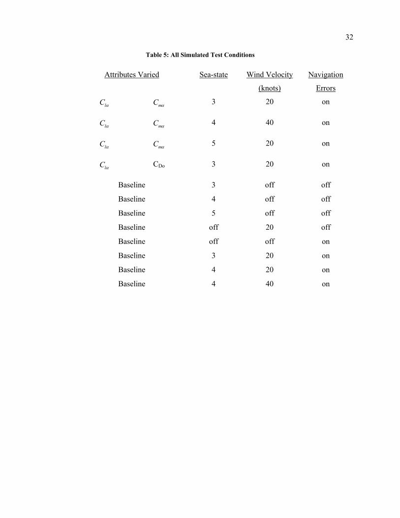
Each of these sets of 100,000 simulation runs was then repeated for varying sea-states,
wind conditions, actuator dynamics, and the cross dependencies of airplane aerodynamic
attributes. The following table lists the test conditions.
32
Table 5: All Simulated Test Conditions
Attributes Varied Sea-state Wind Velocity
(knots)
Navigation
Errors
lC α mC α 3 20 on
lC α mC α 4 40 on
lC α mC α 5 20 on
lC α CDo 3 20 on
Baseline 3 off off
Baseline 4 off off
Baseline 5 off off
Baseline off 20 off
Baseline off off on
Baseline 3 20 on
Baseline 4 20 on
Baseline 4 40 on
33
RESULTS AND DISCUSSION
The following discussion progresses from analysis on single simulation runs, through the
influence and sensitivity to the three sources of disturbances, to specific conclusions bounding
suitable aircraft characteristics based on statistics from many simulations. The primary figures
of merit are the boarding rate and landing dispersion requirements previously presented in Table
1. Secondary figures of merit derived from other structural and actuator limits, including RMS
control power and standard deviation of pitch angle, are also discussed. The influence of three
aircraft characteristics, namely lift-curve slope, longitudinal stability, and coefficient of drag on
these performance metrics were analyzed. For ease of interpretation, all graphics in this section
are standardized such that desirable performance is in the direction of the blue and undesirable
performance is in the direction of the red.
SINGLE SIMULATION RUNS
PRELIMINARY RESULTS (LQR)
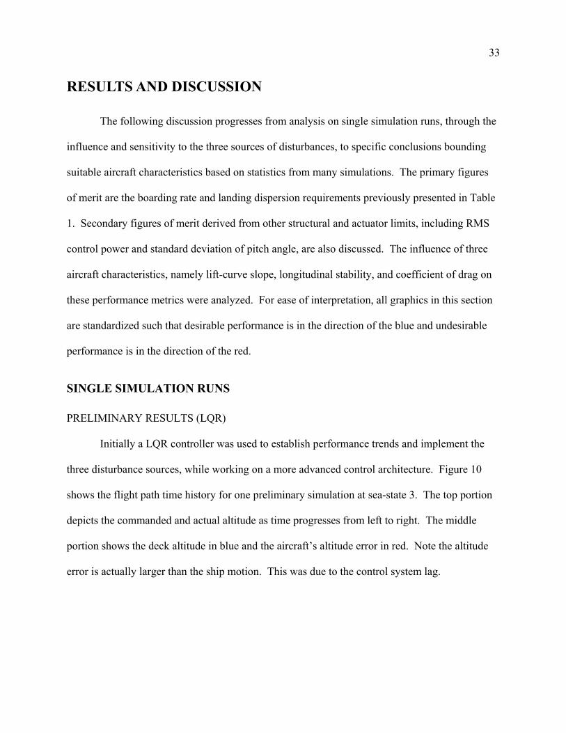
Initially a LQR controller was used to establish performance trends and implement the
three disturbance sources, while working on a more advanced control architecture. Figure 10
shows the flight path time history for one preliminary simulation at sea-state 3. The top portion
depicts the commanded and actual altitude as time progresses from left to right. The middle
portion shows the deck altitude in blue and the aircraft’s altitude error in red. Note the altitude
error is actually larger than the ship motion. This was due to the control system lag.
34
Figure 10: Preliminary Single Simulation Flight Path and Error
This magnitude of error was unacceptable. An altitude error of 10 feet mapped onto the
landing area produces a landing error of 163.5 feet. Although the performance was so poor that
no further results will be presented, several trends were established. The LQR controller was
sensitive to sea-state, but performed very well when only the navigation and gust error sources
were turned on. Lift curve slope was shown to be the dominant factor in landing performance
while longitudinal stability and drag had little to no effect. Also, the effects of bandwidth limits
on the control actuators were tested. Landing performance decreased as actuator speed
decreased, but the reduction in performance was small even with tight bandwidth limits.
35
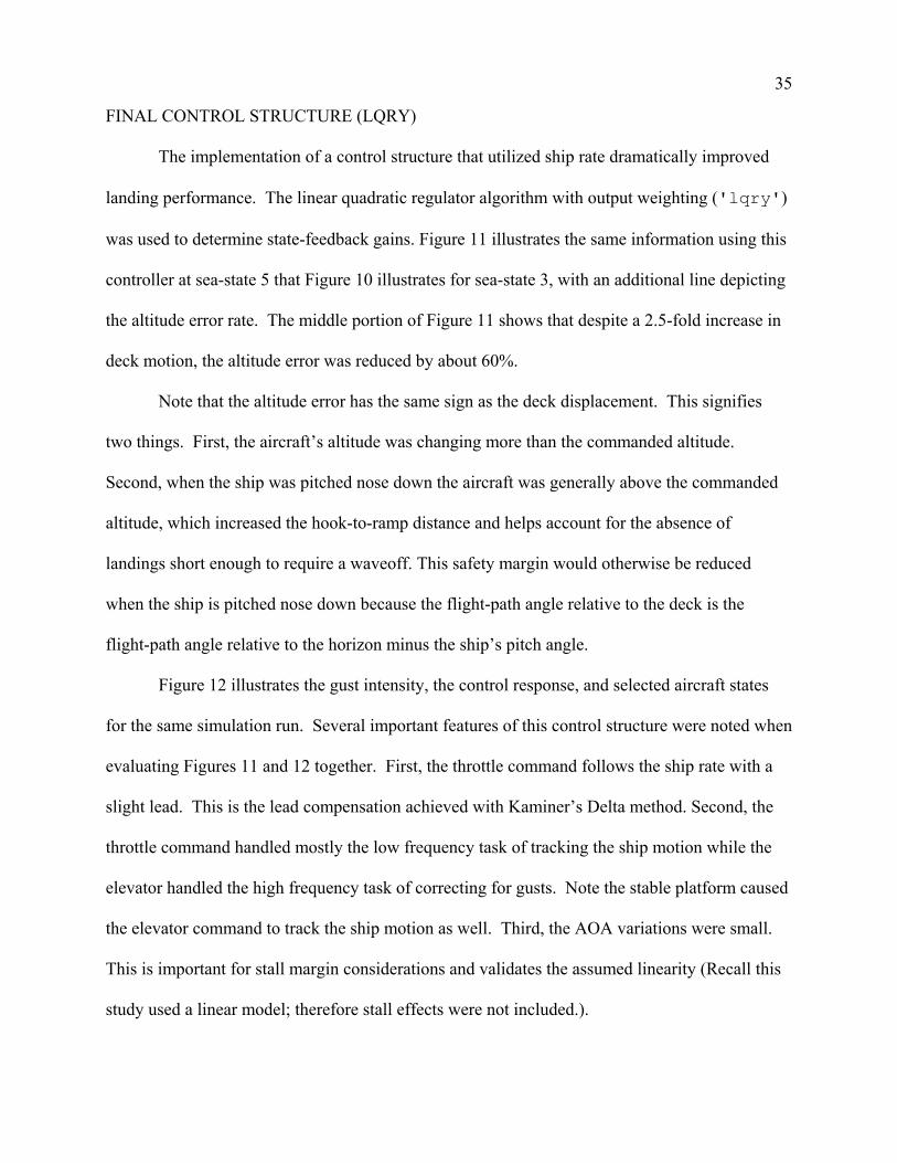
FINAL CONTROL STRUCTURE (LQRY)
The implementation of a control structure that utilized ship rate dramatically improved
landing performance. The linear quadratic regulator algorithm with output weighting ('lqry')
was used to determine state-feedback gains. Figure 11 illustrates the same information using this
controller at sea-state 5 that Figure 10 illustrates for sea-state 3, with an additional line depicting
the altitude error rate. The middle portion of Figure 11 shows that despite a 2.5-fold increase in
deck motion, the altitude error was reduced by about 60%.
Note that the altitude error has the same sign as the deck displacement. This signifies
two things. First, the aircraft’s altitude was changing more than the commanded altitude.
Second, when the ship was pitched nose down the aircraft was generally above the commanded
altitude, which increased the hook-to-ramp distance and helps account for the absence of
landings short enough to require a waveoff. This safety margin would otherwise be reduced
when the ship is pitched nose down because the flight-path angle relative to the deck is the
flight-path angle relative to the horizon minus the ship’s pitch angle.
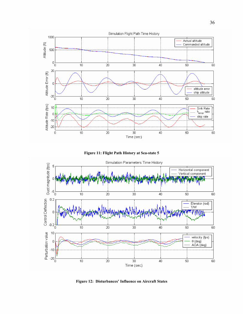
Figure 12 illustrates the gust intensity, the control response, and selected aircraft states
for the same simulation run. Several important features of this control structure were noted when
evaluating Figures 11 and 12 together. First, the throttle command follows the ship rate with a
slight lead. This is the lead compensation achieved with Kaminer’s Delta method. Second, the
throttle command handled mostly the low frequency task of tracking the ship motion while the
elevator handled the high frequency task of correcting for gusts. Note the stable platform caused
the elevator command to track the ship motion as well. Third, the AOA variations were small.
This is important for stall margin considerations and validates the assumed linearity (Recall this
study used a linear model; therefore stall effects were not included.).
36
Figure 11: Flight Path History at Sea-state 5
Figure 12: Disturbances’ Influence on Aircraft States
37
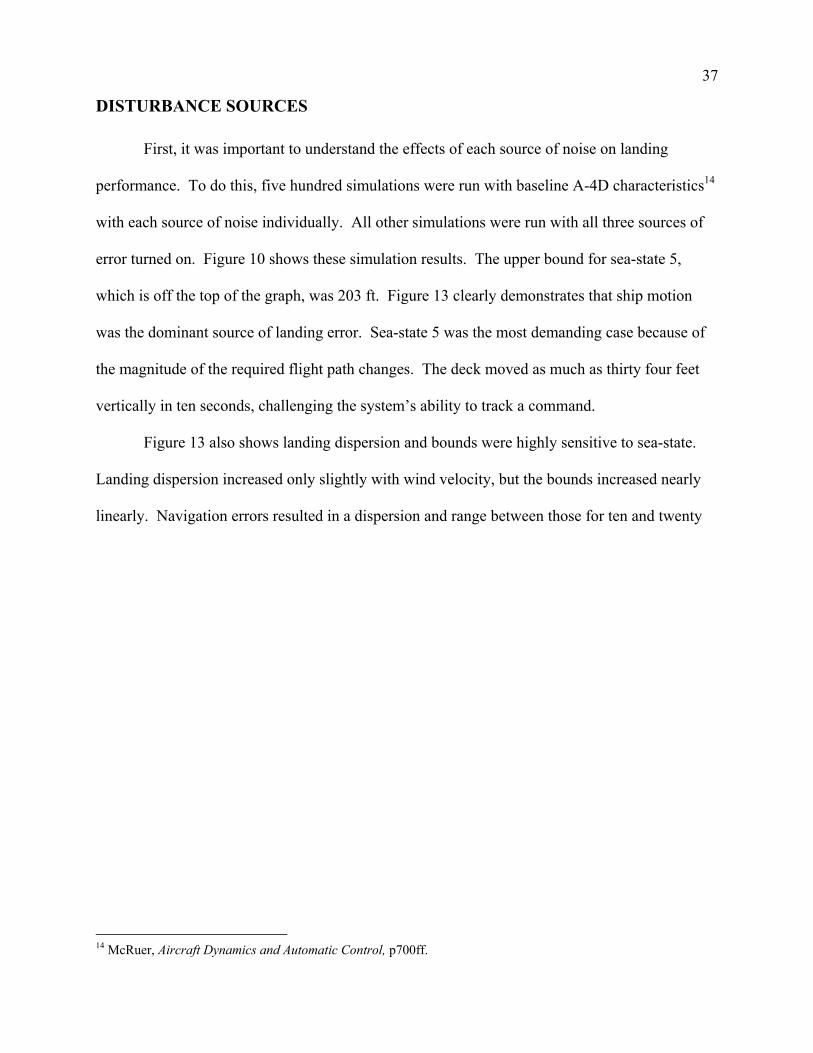
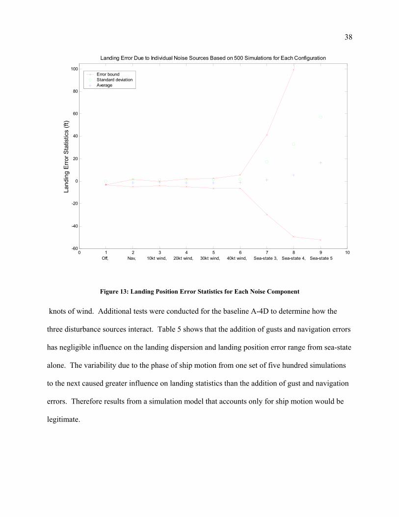
DISTURBANCE SOURCES
First, it was important to understand the effects of each source of noise on landing
performance. To do this, five hundred simulations were run with baseline A-4D characteristics14
with each source of noise individually. All other simulations were run with all three sources of
error turned on. Figure 10 shows these simulation results. The upper bound for sea-state 5,
which is off the top of the graph, was 203 ft. Figure 13 clearly demonstrates that ship motion
was the dominant source of landing error. Sea-state 5 was the most demanding case because of
the magnitude of the required flight path changes. The deck moved as much as thirty four feet
vertically in ten seconds, challenging the system’s ability to track a command.
Figure 13 also shows landing dispersion and bounds were highly sensitive to sea-state.
Landing dispersion increased only slightly with wind velocity, but the bounds increased nearly
linearly. Navigation errors resulted in a dispersion and range between those for ten and twenty
14 McRuer, Aircraft Dynamics and Automatic Control, p700ff.
38
0 1 2 3 4 5 6 7 8 9 10-60
-40
-20
0
20
40
60
80
100La
ndin
g Er
ror S
tatis
tics
(ft)
Landing Error Due to Individual Noise Sources Based on 500 Simulations for Each Configuration
Off, Nav, 10kt wind, 20kt wind, 30kt wind, 40kt wind, Sea-state 3, Sea-state 4, Sea-state 5
Error bound Standard deviationAverage
Figure 13: Landing Position Error Statistics for Each Noise Component
knots of wind. Additional tests were conducted for the baseline A-4D to determine how the
three disturbance sources interact. Table 5 shows that the addition of gusts and navigation errors
has negligible influence on the landing dispersion and landing position error range from sea-state
alone. The variability due to the phase of ship motion from one set of five hundred simulations
to the next caused greater influence on landing statistics than the addition of gust and navigation
errors. Therefore results from a simulation model that accounts only for ship motion would be
legitimate.

39
Table 6: Combination Effects of Disturbance Sources
Condition Std. Dev (ft) Error Range (ft)
Sea-state 3 17.4 70.8 Sea-state 4 33.2 148.8
Sea-state 3, 20wind, nav 17.3 72.7 Sea-state 4, 20wind, nav 33.7 147.0 Sea-state 4, 40wind, nav 33.1 151.8
INFLUENCE OF LIFT CURVE SLOPE AND LONGITUDINAL STABILITY
The combined influence of longitudinal stability and lift curve slope was
evaluated by a combined total of three hundred thousand simulation runs. The lift curve slope
was varied from six-tenths per radian to six per radian in increments of six-tenths per radian. Lift
curve slope varies with wing sweep angle and aspect ratio, with lower values of aspect ratio and
aft wing sweeps resulting in lower values of lift curve slope. The longitudinal stability was
varied from negative sixty-five hundredths (stable) to twenty-five hundredths (slightly unstable)
in increments of one tenth. Longitudinal stability is dependent on the location of the center of
gravity relative to the wing’s aerodynamic center, where moving the center of gravity aft
decreases stability. All other attributes were those for the baseline A-4D in the landing
configuration, including a lift to drag ratio of approximately two. At each combination, one
thousand simulated landings were performed for each sea-state and the landing statistics captured
as discussed previously.
BOARDING RATE AND LANDING DISPERSION
The sea-state 3 simulations for all modeled configurations had error bounds within the
acceptable landing area. This means that if landing position were the only criterion, the
autonomous system would have a perfect boarding rate for any aircraft for all conditions up to
40
and including sea-state 3. Sea-state 3 simulation results yielded no further information and are
not shown.
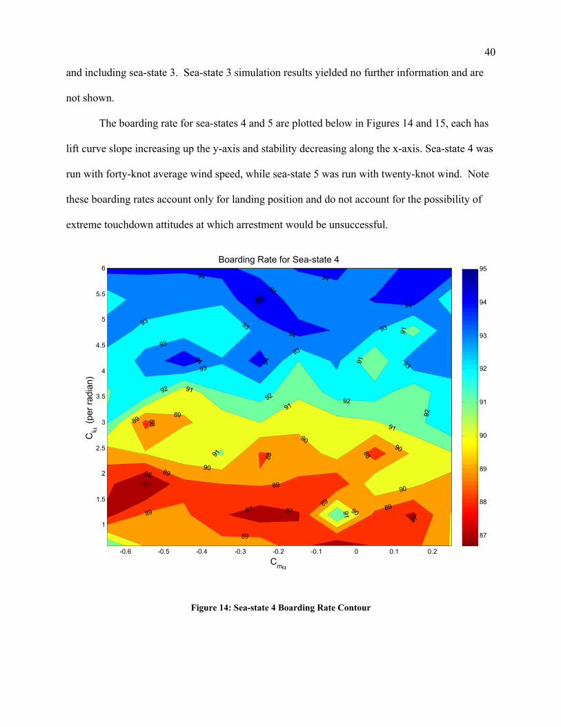
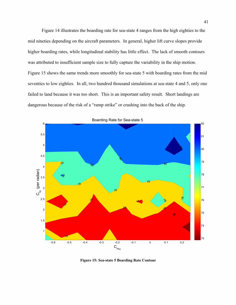
The boarding rate for sea-states 4 and 5 are plotted below in Figures 14 and 15, each has
lift curve slope increasing up the y-axis and stability decreasing along the x-axis. Sea-state 4 was
run with forty-knot average wind speed, while sea-state 5 was run with twenty-knot wind. Note
these boarding rates account only for landing position and do not account for the possibility of
extreme touchdown attitudes at which arrestment would be unsuccessful.
87
88
89
90
91
92
93
94
95
-0.6 -0.5 -0.4 -0.3 -0.2 -0.1 0 0.1 0.2
1
1.5
2
2.5
3
3.5
4
4.5
5
5.5
6
Cmα
Cl α
(per
radi
an)
Boarding Rate for Sea-state 4
88
8989
89
89
90
90
90
90
91
91
91
92
929292
93
93
93
93
93
9393
89
89
94
94
94
94
8989
87 87 90
91
94
94 94
91
88
91
88
88
87
95
91
Figure 14: Sea-state 4 Boarding Rate Contour
41
Figure 14 illustrates the boarding rate for sea-state 4 ranges from the high eighties to the
mid nineties depending on the aircraft parameters. In general, higher lift curve slopes provide
higher boarding rates, while longitudinal stability has little effect. The lack of smooth contours
was attributed to insufficient sample size to fully capture the variability in the ship motion.
Figure 15 shows the same trends more smoothly for sea-state 5 with boarding rates from the mid
seventies to low eighties. In all, two hundred thousand simulations at sea-state 4 and 5, only one
failed to land because it was too short. This is an important safety result. Short landings are
dangerous because of the risk of a “ramp strike” or crashing into the back of the ship.
73
74
75
76
77
78
79
80
81
82
-0.6 -0.5 -0.4 -0.3 -0.2 -0.1 0 0.1 0.2
1
1.5
2
2.5
3
3.5
4
4.5
5
5.5
6
Cmα
Cl α
(per
radi
an)
Boarding Rate for Sea-state 5
7676
76
7878
78
78
78 80
80
80
76
82
74
78
74
80
Figure 15: Sea-state 5 Boarding Rate Contour
42
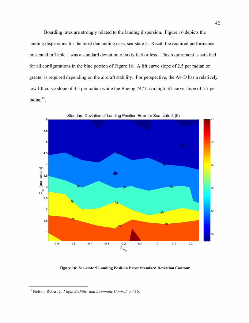
Boarding rates are strongly related to the landing dispersion. Figure 16 depicts the
landing dispersions for the most demanding case, sea-state 5. Recall the required performance
presented in Table 1 was a standard deviation of sixty feet or less. This requirement is satisfied
for all configurations in the blue portion of Figure 16. A lift curve slope of 2.5 per radian or
greater is required depending on the aircraft stability. For perspective, the A4-D has a relatively
low lift curve slope of 3.5 per radian while the Boeing 747 has a high lift-curve slope of 5.7 per
radian15.
50
55
60
65
70
75
-0.6 -0.5 -0.4 -0.3 -0.2 -0.1 0 0.1 0.2
1
1.5
2
2.5
3
3.5
4
4.5
5
5.5
6
Cmα
Cl α
(per
radi
an)
Standard Deviation of Landing Position Error for Sea-state 5 (ft)
50
5555
55
60 60 60
65 65
65
70
7070
50
Figure 16: Sea-state 5 Landing Position Error Standard Deviation Contour
15 Nelson, Robert C. Flight Stability and Automatic Control, p. 416.
43
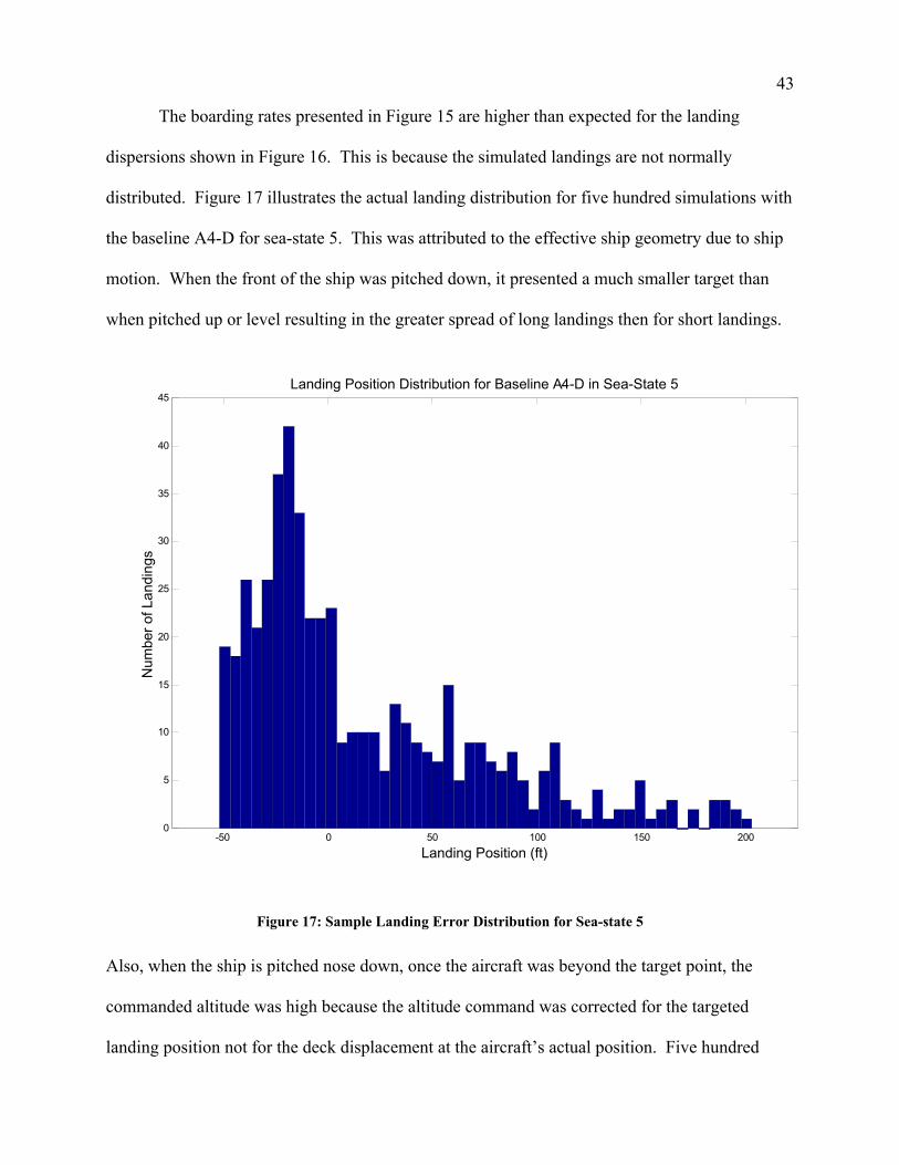
The boarding rates presented in Figure 15 are higher than expected for the landing
dispersions shown in Figure 16. This is because the simulated landings are not normally
distributed. Figure 17 illustrates the actual landing distribution for five hundred simulations with
the baseline A4-D for sea-state 5. This was attributed to the effective ship geometry due to ship
motion. When the front of the ship was pitched down, it presented a much smaller target than
when pitched up or level resulting in the greater spread of long landings then for short landings.
-50 0 50 100 150 2000
5
10
15
20
25
30
35
40
45
Num
ber o
f Lan
ding
s
Landing Position (ft)
Landing Position Distribution for Baseline A4-D in Sea-State 5
Figure 17: Sample Landing Error Distribution for Sea-state 5
Also, when the ship is pitched nose down, once the aircraft was beyond the target point, the
commanded altitude was high because the altitude command was corrected for the targeted
landing position not for the deck displacement at the aircraft’s actual position. Five hundred
44
simulations were run with the commanded altitude corrected for the aircraft’s actual position to
test its influence on performance. The standard deviation decreased slightly and the maximum
error decreased by more than ten percent, but there was no change in boarding rate, therefore
previous simulations were not redone.
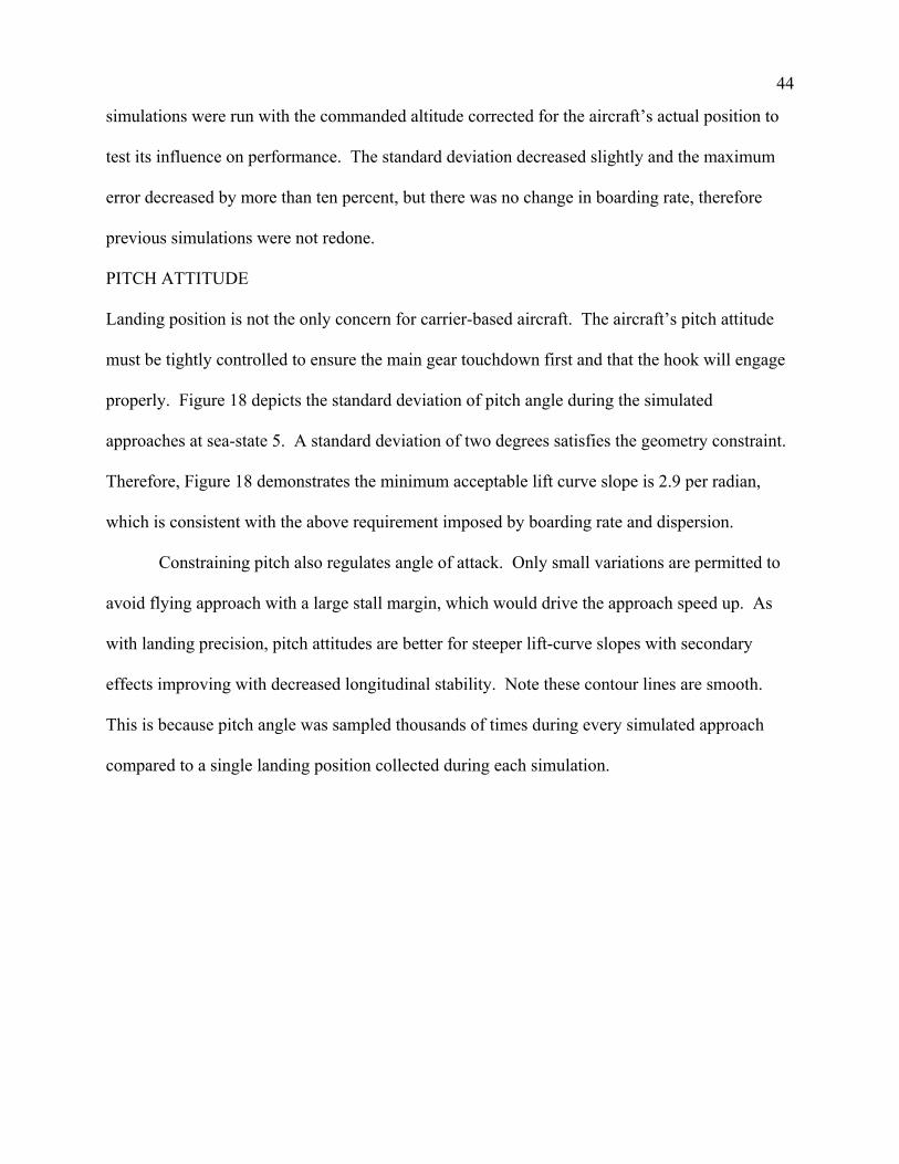
PITCH ATTITUDE
Landing position is not the only concern for carrier-based aircraft. The aircraft’s pitch attitude
must be tightly controlled to ensure the main gear touchdown first and that the hook will engage
properly. Figure 18 depicts the standard deviation of pitch angle during the simulated
approaches at sea-state 5. A standard deviation of two degrees satisfies the geometry constraint.
Therefore, Figure 18 demonstrates the minimum acceptable lift curve slope is 2.9 per radian,
which is consistent with the above requirement imposed by boarding rate and dispersion.
Constraining pitch also regulates angle of attack. Only small variations are permitted to
avoid flying approach with a large stall margin, which would drive the approach speed up. As
with landing precision, pitch attitudes are better for steeper lift-curve slopes with secondary
effects improving with decreased longitudinal stability. Note these contour lines are smooth.
This is because pitch angle was sampled thousands of times during every simulated approach
compared to a single landing position collected during each simulation.
45
0.5
1
1.5
2
2.5
3
3.5
4
4.5
5
5.5
6
-0.6 -0.5 -0.4 -0.3 -0.2 -0.1 0 0.1 0.2
1
1.5
2
2.5
3
3.5
4
4.5
5
5.5
6
Cmα
Cl α
(per
radi
an)
Standard Deviation of Pitch Angle, θ (deg), for Sea-state 5
1.751.75
1.75
22
2
2.5
2.52.53 3
34
46
Figure 18: Sea-state 5 Pitch Angle Standard Deviation Contour
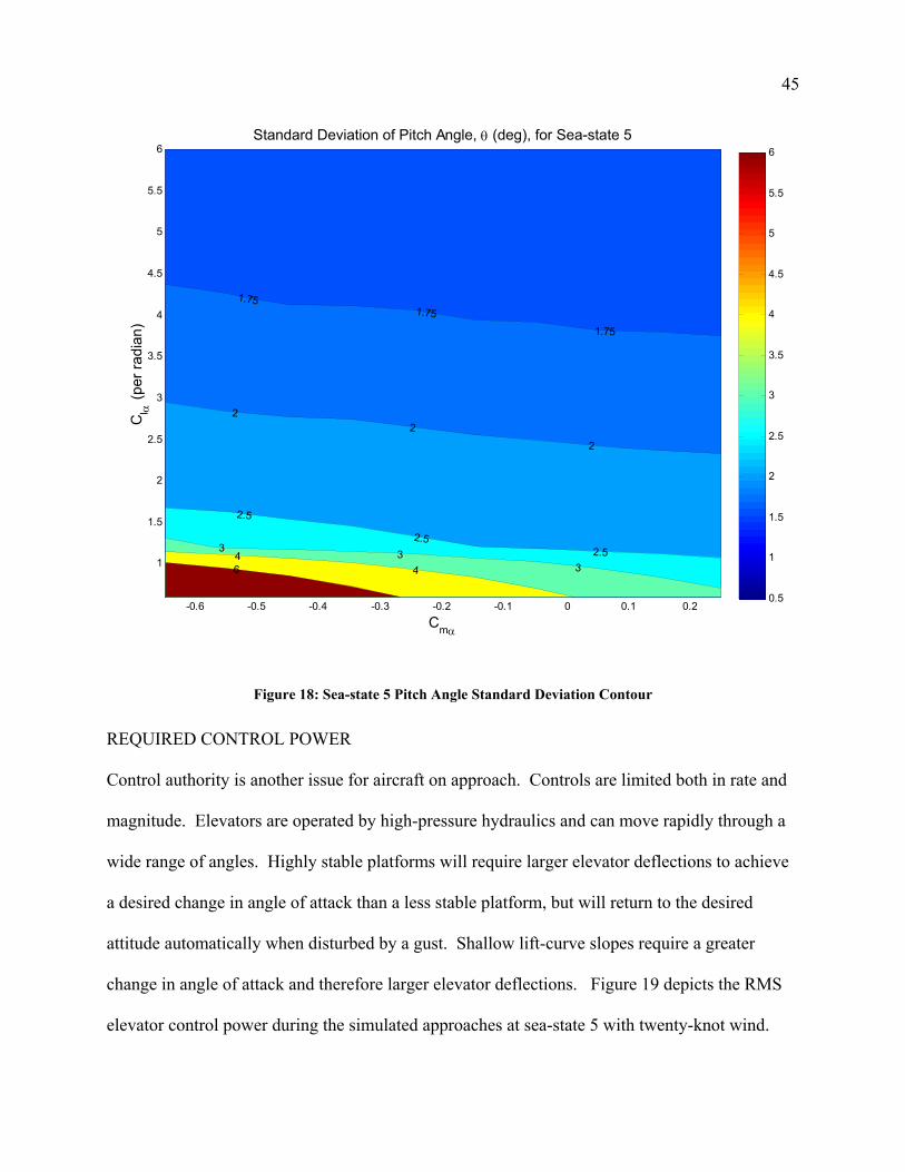
REQUIRED CONTROL POWER
Control authority is another issue for aircraft on approach. Controls are limited both in rate and
magnitude. Elevators are operated by high-pressure hydraulics and can move rapidly through a
wide range of angles. Highly stable platforms will require larger elevator deflections to achieve
a desired change in angle of attack than a less stable platform, but will return to the desired
attitude automatically when disturbed by a gust. Shallow lift-curve slopes require a greater
change in angle of attack and therefore larger elevator deflections. Figure 19 depicts the RMS
elevator control power during the simulated approaches at sea-state 5 with twenty-knot wind.
46
1
1.5
2
2.5
3
3.5
4
-0.6 -0.5 -0.4 -0.3 -0.2 -0.1 0 0.1 0.2
1
1.5
2
2.5
3
3.5
4
4.5
5
5.5
6
Cmα
Cl α
(per
radi
an)
RMS Elevator Control Power for Sea-state 5 (deg)
1.25
1.25
1.5
1.75
2
1.25
2.53
1
Figure 19: Sea-state 5 RMS Elevator Control Power
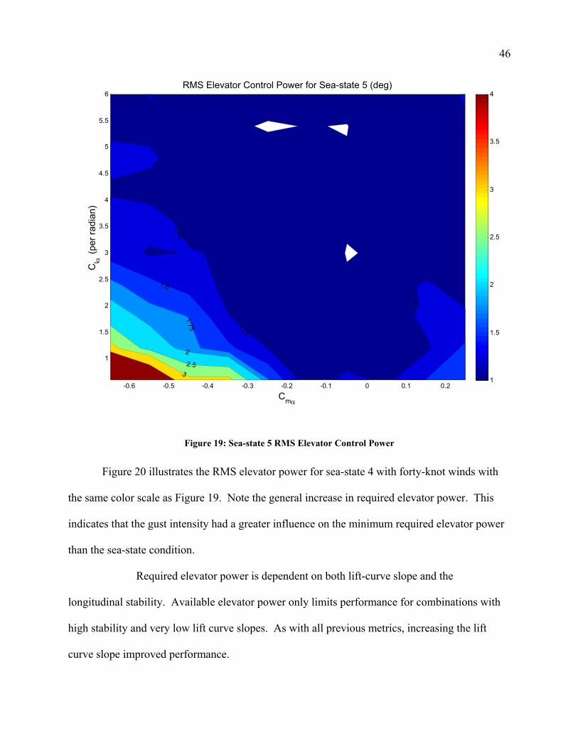
Figure 20 illustrates the RMS elevator power for sea-state 4 with forty-knot winds with
the same color scale as Figure 19. Note the general increase in required elevator power. This
indicates that the gust intensity had a greater influence on the minimum required elevator power
than the sea-state condition.
Required elevator power is dependent on both lift-curve slope and the
longitudinal stability. Available elevator power only limits performance for combinations with
high stability and very low lift curve slopes. As with all previous metrics, increasing the lift
curve slope improved performance.
47
1
1.5
2
2.5
3
3.5
4
-0.6 -0.5 -0.4 -0.3 -0.2 -0.1 0 0.1 0.2
1
1.5
2
2.5
3
3.5
4
4.5
5
5.5
6
Cmα
Cl α
(per
radi
an)
RMS Elevator Control Power for Sea-state 4 (deg)
1.75
2
2
2
1.5135
1.51
35
1.5135
2.52
2
3
1.5135
1.5135
2
1.513
5
2
2
Figure 20: Sea-state 4 RMS Elevator Control Power
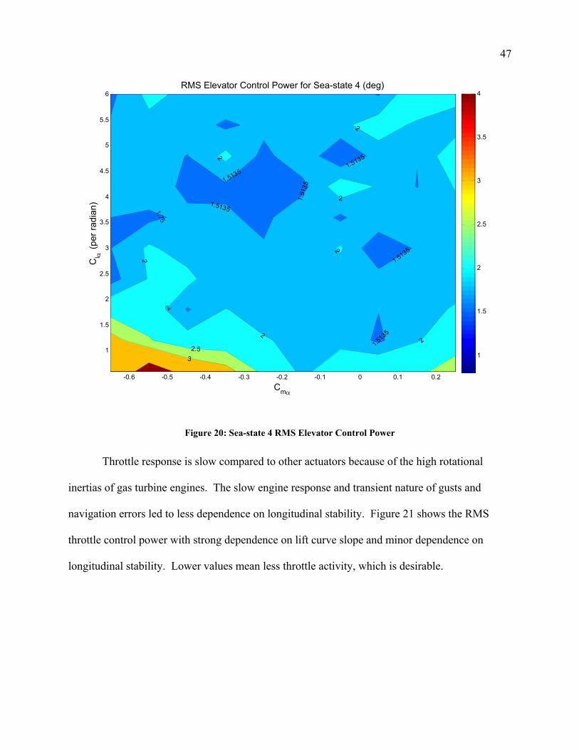
Throttle response is slow compared to other actuators because of the high rotational
inertias of gas turbine engines. The slow engine response and transient nature of gusts and
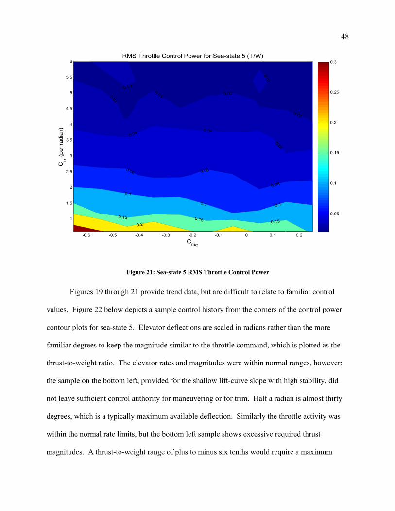
navigation errors led to less dependence on longitudinal stability. Figure 21 shows the RMS
throttle control power with strong dependence on lift curve slope and minor dependence on
longitudinal stability. Lower values mean less throttle activity, which is desirable.
48
0.05
0.1
0.15
0.2
0.25
0.3
-0.6 -0.5 -0.4 -0.3 -0.2 -0.1 0 0.1 0.2
1
1.5
2
2.5
3
3.5
4
4.5
5
5.5
6
Cmα
Cl α
(per
radi
an)
RMS Throttle Control Power for Sea-state 5 (T/W)
0.03
0.03 0.03
0.03
0.04 0.04
0.04
0.06 0.06
0.06
0.1
0.1 0.1
0.15 0.15 0.150.2
0.03
0.03
Figure 21: Sea-state 5 RMS Throttle Control Power
Figures 19 through 21 provide trend data, but are difficult to relate to familiar control
values. Figure 22 below depicts a sample control history from the corners of the control power
contour plots for sea-state 5. Elevator deflections are scaled in radians rather than the more
familiar degrees to keep the magnitude similar to the throttle command, which is plotted as the
thrust-to-weight ratio. The elevator rates and magnitudes were within normal ranges, however;
the sample on the bottom left, provided for the shallow lift-curve slope with high stability, did
not leave sufficient control authority for maneuvering or for trim. Half a radian is almost thirty
degrees, which is a typically maximum available deflection. Similarly the throttle activity was
within the normal rate limits, but the bottom left sample shows excessive required thrust
magnitudes. A thrust-to-weight range of plus to minus six tenths would require a maximum
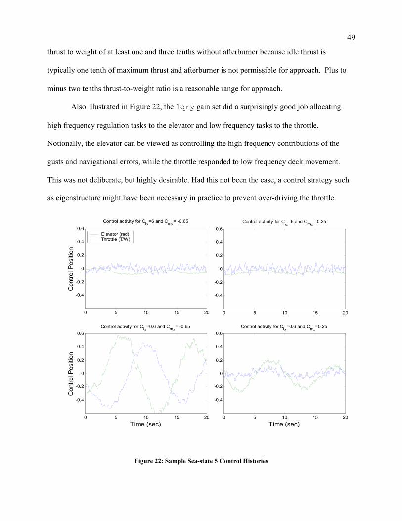
49
thrust to weight of at least one and three tenths without afterburner because idle thrust is
typically one tenth of maximum thrust and afterburner is not permissible for approach. Plus to
minus two tenths thrust-to-weight ratio is a reasonable range for approach.
Also illustrated in Figure 22, the lqry gain set did a surprisingly good job allocating
high frequency regulation tasks to the elevator and low frequency tasks to the throttle.
Notionally, the elevator can be viewed as controlling the high frequency contributions of the
gusts and navigational errors, while the throttle responded to low frequency deck movement.
This was not deliberate, but highly desirable. Had this not been the case, a control strategy such
as eigenstructure might have been necessary in practice to prevent over-driving the throttle.
0 5 10 15 20
-0.4
-0.2
0
0.2
0.4
0.6
Time (sec)
Control activity for Clα=0.6 and Cmα= -0.65
Con
trol P
ositi
on
0 5 10 15 20
-0.4
-0.2
0
0.2
0.4
0.6
Con
trol P
ositi
on
Control activity for Clα=6 and Cmα= -0.65
Elevator (rad)Throttle (T/W)
0 5 10 15 20
-0.4
-0.2
0
0.2
0.4
0.6Control activity for Clα=6 and Cmα= 0.25
0 5 10 15 20
-0.4
-0.2
0
0.2
0.4
0.6Control activity for Clα=0.6 and Cmα=0.25
Time (sec)
Figure 22: Sample Sea-state 5 Control Histories
50
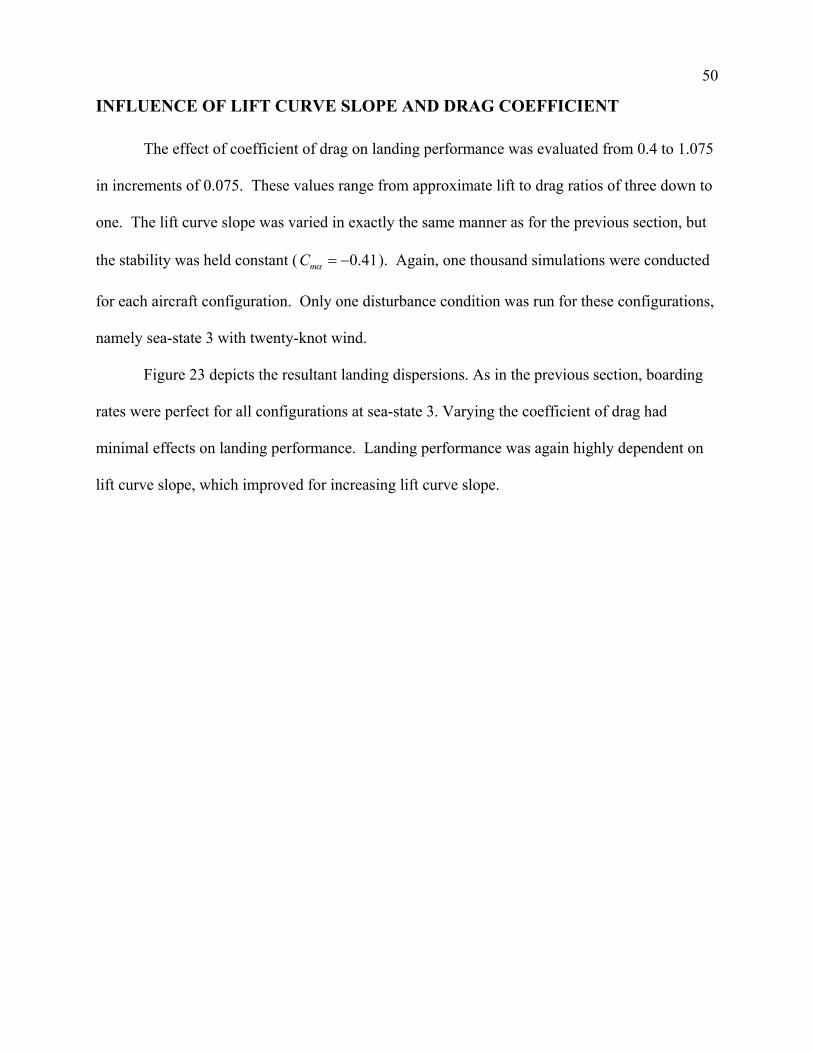
INFLUENCE OF LIFT CURVE SLOPE AND DRAG COEFFICIENT
The effect of coefficient of drag on landing performance was evaluated from 0.4 to 1.075
in increments of 0.075. These values range from approximate lift to drag ratios of three down to
one. The lift curve slope was varied in exactly the same manner as for the previous section, but
the stability was held constant ( 0.41mC α = − ). Again, one thousand simulations were conducted
for each aircraft configuration. Only one disturbance condition was run for these configurations,
namely sea-state 3 with twenty-knot wind.
Figure 23 depicts the resultant landing dispersions. As in the previous section, boarding
rates were perfect for all configurations at sea-state 3. Varying the coefficient of drag had
minimal effects on landing performance. Landing performance was again highly dependent on
lift curve slope, which improved for increasing lift curve slope.
51
15
16
17
18
19
20
21
22
0.4 0.5 0.6 0.7 0.8 0.9 1
1
1.5
2
2.5
3
3.5
4
4.5
5
5.5
6
CDo
Cl α
(per
radi
an)
Standard Deviation of Landing Position Error for Sea-state 3 (ft)
1515
15
1616
16 16
1617
17 17
18
18
1819
19 1920
20
202121
212222
Figure 23: Sea-state 3 Landing Position Error Standard Deviation Contour
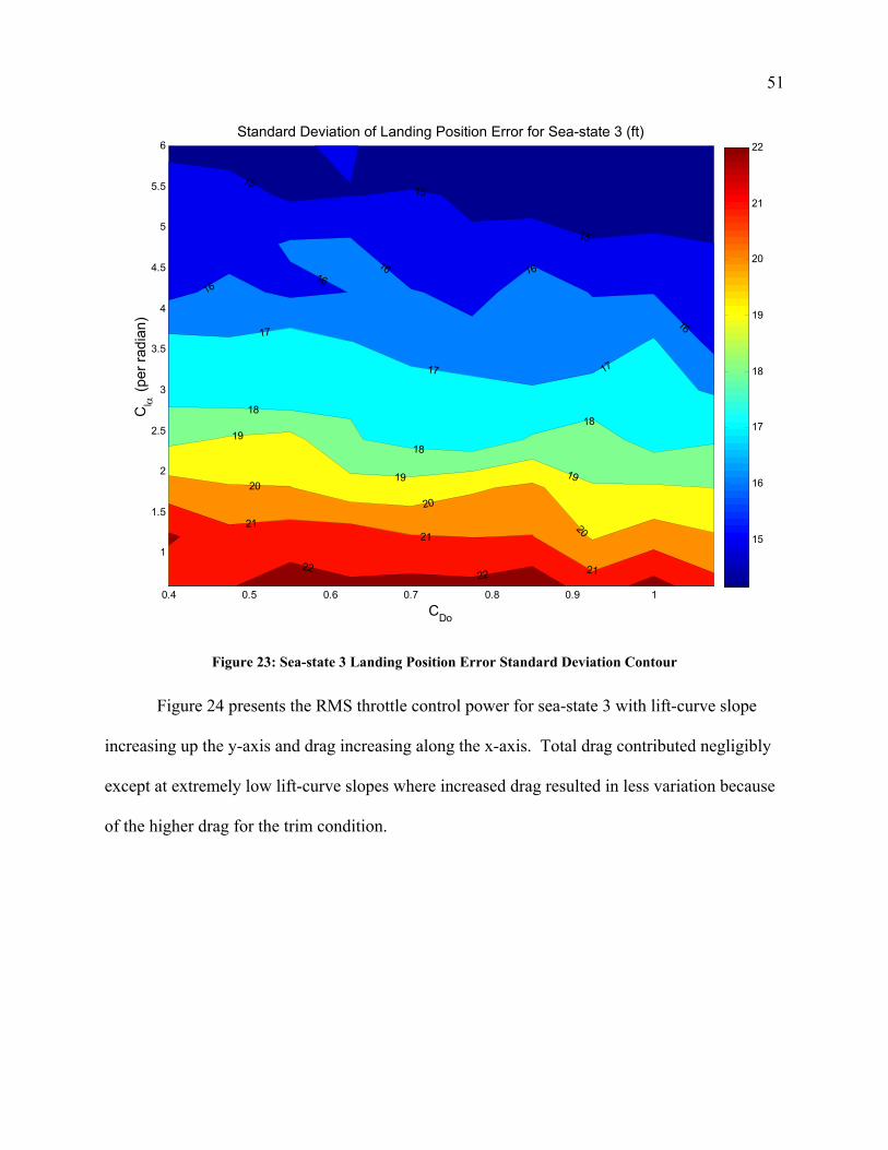
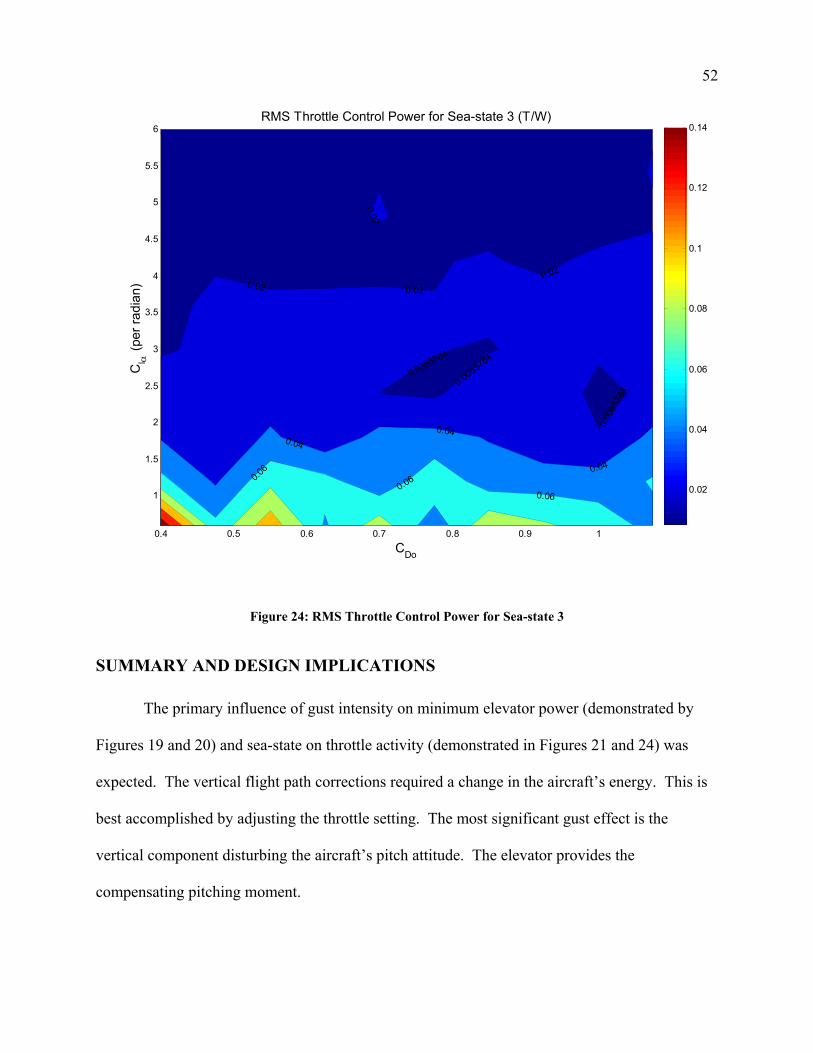
Figure 24 presents the RMS throttle control power for sea-state 3 with lift-curve slope
increasing up the y-axis and drag increasing along the x-axis. Total drag contributed negligibly
except at extremely low lift-curve slopes where increased drag resulted in less variation because
of the higher drag for the trim condition.
52
0.02
0.04
0.06
0.08
0.1
0.12
0.14
0.4 0.5 0.6 0.7 0.8 0.9 1
1
1.5
2
2.5
3
3.5
4
4.5
5
5.5
6
CDo
Cl α
(per
radi
an)
RMS Throttle Control Power for Sea-state 3 (T/W)
0.02 0.020.02
0.040.04
0.040.0
6
0.060.06
0.0085784
0.008
5784
0.00
8578
4
0.02
Figure 24: RMS Throttle Control Power for Sea-state 3
SUMMARY AND DESIGN IMPLICATIONS
The primary influence of gust intensity on minimum elevator power (demonstrated by
Figures 19 and 20) and sea-state on throttle activity (demonstrated in Figures 21 and 24) was
expected. The vertical flight path corrections required a change in the aircraft’s energy. This is
best accomplished by adjusting the throttle setting. The most significant gust effect is the
vertical component disturbing the aircraft’s pitch attitude. The elevator provides the
compensating pitching moment.
53
The longitudinal stability had little influence on landing performance. This was expected
because the stability determines the aircraft’s open-loop response (response in the absence of
control inputs) to disturbances. Because the automatic control system was continuously updating
the control commands, the natural response played a negligible role in landing performance.
Designing an aircraft to be unstable has approach speed and maximum landing weight benefits.
The most unstable configurations presented in this section were the most desirable for every
figure of merit evaluated. Within the scope of the tested range, this study does not indicate a
limit on the amount of instability suitable for an autonomous carrier-based aircraft.
The drag coefficient had little effect on landing performance for the same reasons as
longitudinal stability. For some manned aircraft, speedbrakes are deployed to allow approach to
be flown on the front-side of the power curve where speed is stable rather than the back side of
the power curve where speed is unstable. The automatic control system makes the small updates
continuously. Consequently, the aircraft’s natural stability is unimportant. This insensitivity to
drag coefficient leaves a decision on speed brakes completely to the designer, and means that the
landing dispersion would be robust to variations in drag, such as might be caused by combat
damage or the carriage of external stores.
The lift curve slope was the dominant factor in all aspects of performance for the carrier-
landing task; increasing the lift curve slope improved performance. This was the expected result
because tracking the commanded altitude involved nothing more than shifting the airplane’s
flight path vertically about a trim condition, in our case a ramp representing the glide slope,
perturbed by our diverse disturbances. A vertical shift in the flight path required a change in lift
coefficient because the airspeed was tightly regulated as required. The lift curve slope represents
the sensitivity of flight path angle change to change in AOA. The lift curve slope directly
54
determined the required change in AOA for the desired change in lift thereby determining all of
the performance characteristics previously discussed. Future UCAV designs must carefully
weigh the landing performance benefits of a high lift curve slope, with a minimum of 2.9 per
radian, against other operational performance requirements. The minimum lift curve slope
requirement constrains the minimum aspect ratio and the maximum wing sweep angle, the two
primary geometric attributes of an aircraft.
CONCLUSIONS
Several specific conclusions were reached based on this simulation study. They are as
follows:
a. Navigation errors, using the state-of-the-art satellite based systems, are small
and result in negligible landing errors as demonstrated in Figure 13 and Table
6.
b. Gust intensity influences the required RMS elevator power, but results in
negligible landing errors when modeled concurrently with any significant sea-
state.
c. Ship motion is the dominant cause of landing errors. Landing dispersion and
boarding rates are highly dependent on sea-state.
d. Longitudinal stability and drag coefficient has negligible influence on landing
precision and control requirements. No limit on instability or range of
acceptable drag coefficient was indicated.

55
e. Lift curve slope is the dominant aircraft attribute for all landing performance
criteria and each improves with increasing lift curve slope. The minimum lift
curve slope for suitable longitudinal landing performance is 2.9 per radian.
RECOMMENDATIONS
The effect of direct lift control (DLC) should be investigated. DLC acts in the direction
of desired control, while throttle and elevator control altitude only indirectly. Also, because
DLC is a small, light-weight control surface it is capable of very high bandwidth activity. DLC
will likely reduce the strong dependency upon lift curve slope since it provides direct control
over the flight path angle.
An investigation should be conducted to determine the performance of alternative control
structures such as eigenstructure assignment or an LQR controller that incorporates the known
ship accelerations in addition to the ship rates and position. The lqry gains used in this study
automatically assigned high frequency control to the elevator and low frequency control to
throttle, but this may not be the case when a third control input is introduced to the system.
An investigation should be conducted for lateral mode aircraft dynamics. This is a more
complex problem because of the coupling of the airplane's lateral and directional axes, plus the
coupling of the ship's lateral and directional axes.
BIBLIOGRAPHY Clark, Vern. “Sea Power 21,” Proceedings. U.S. Naval Institute, October, 2002 (available
from http://www.usni.org/Proceedings/articles02/proCNO10.htm ).
Etkin, Bernard. Dynamics of Flight. John Wiley & Sons, 1959.
56
Heffley, Robert, Outer-Loop Control Factors For Carrier Aircraft. Report number: RHE-
NAV-90-TR-1, Naval Air Systems Command, DEC 90.
Kaminer, I., A.M. Pascoal, P.P. Khargonekar, and E. Coleman, ``A Velocity Algorithm for the
Implementation of Nonlinear Gain-Scheduled Controllers'', Automatica, Vol. 31, pp.
1185--1191,1995.
McRuer, Ashkenas, and Graham. Aircraft Dynamics and Automatic Control. Princeton
University Press, 1973.
Mulder, J.A. and Van der Vaart, J.C. “Lecture Notes Dictaat D-47: Aircraft Response to
Atmospheric Turbulence”, Delft University, 1993.
Nelson, Robert C. Flight Stability and Automatic Control. Second ed. McGraw-Hill, 1998.
Rudowsky et al. Review of the Carrier Approach Criteria for Carrier-Based Aircraft Phase I;
Final Report. Report number: NAWCADPAX/TR-2002/71, Naval Air Systems
Command, OCT 02.
Schug et al. "Guidance and Control for Shipboard Automatic Landing Using GPS," draft report.
U.S. Naval Test Pilot School Flight Test Manual No. 103, Fixed Wing Stability and Control:
Theory and Flight Test Techniques. Patuxent River, 1997.
Waters et al., "Test Results of an F/A-18 Automatic Carrier Landing Using Shipboard Relative
GPS," draft report.
Waters, Jack. Carrier Suitability Department Head, Naval Strike Aircraft Test Squadron. “Ship
Landing Issues” PowerPoint Presentation.
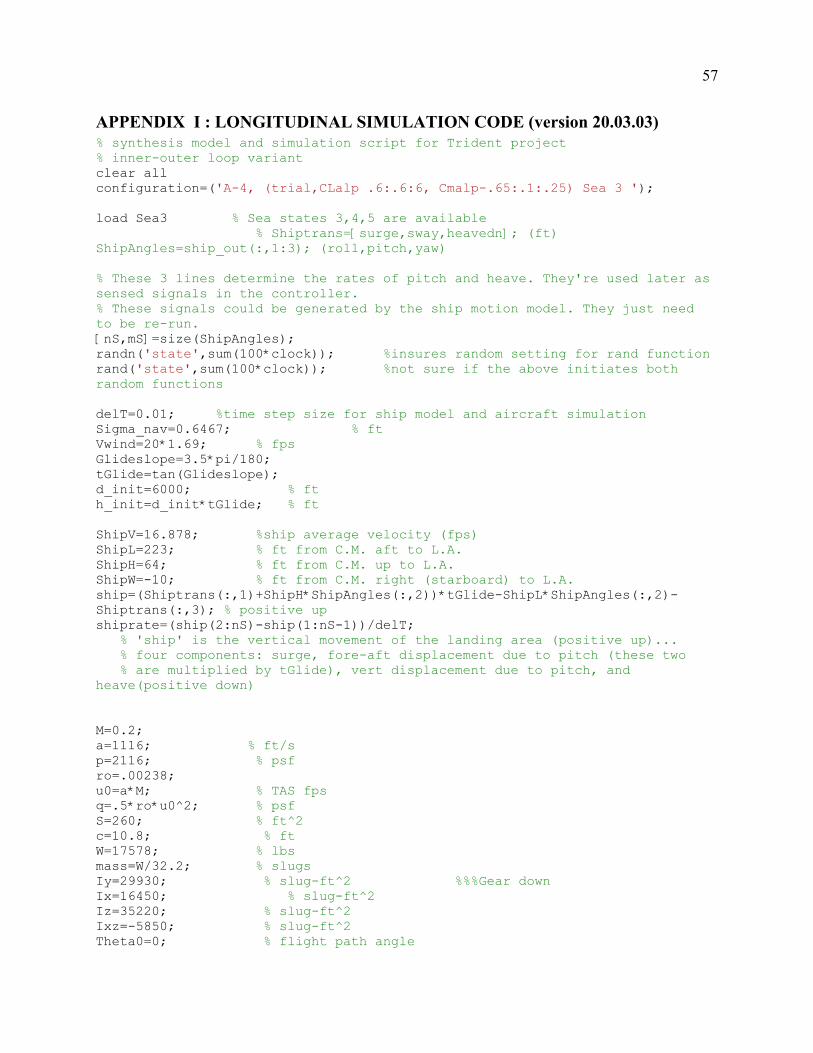
57
APPENDIX I : LONGITUDINAL SIMULATION CODE (version 20.03.03) % synthesis model and simulation script for Trident project % inner-outer loop variant clear all configuration=('A-4, (trial,CLalp .6:.6:6, Cmalp-.65:.1:.25) Sea 3 '); load Sea3 % Sea states 3,4,5 are available % Shiptrans=[surge,sway,heavedn]; (ft) ShipAngles=ship_out(:,1:3); (roll,pitch,yaw) % These 3 lines determine the rates of pitch and heave. They're used later as sensed signals in the controller. % These signals could be generated by the ship motion model. They just need to be re-run. [nS,mS]=size(ShipAngles); randn('state',sum(100*clock)); %insures random setting for rand function rand('state',sum(100*clock)); %not sure if the above initiates both random functions delT=0.01; %time step size for ship model and aircraft simulation Sigma_nav=0.6467; % ft Vwind=20*1.69; % fps Glideslope=3.5*pi/180; tGlide=tan(Glideslope); d_init=6000; % ft h_init=d_init*tGlide; % ft ShipV=16.878; %ship average velocity (fps) ShipL=223; % ft from C.M. aft to L.A. ShipH=64; % ft from C.M. up to L.A. ShipW=-10; % ft from C.M. right (starboard) to L.A. ship=(Shiptrans(:,1)+ShipH*ShipAngles(:,2))*tGlide-ShipL*ShipAngles(:,2)-Shiptrans(:,3); % positive up shiprate=(ship(2:nS)-ship(1:nS-1))/delT; % 'ship' is the vertical movement of the landing area (positive up)... % four components: surge, fore-aft displacement due to pitch (these two % are multiplied by tGlide), vert displacement due to pitch, and heave(positive down) M=0.2; a=1116; % ft/s p=2116; % psf ro=.00238; u0=a*M; % TAS fps q=.5*ro*u0^2; % psf S=260; % ft^2 c=10.8; % ft W=17578; % lbs mass=W/32.2; % slugs Iy=29930; % slug-ft^2 %%%Gear down Ix=16450; % slug-ft^2 Iz=35220; % slug-ft^2 Ixz=-5850; % slug-ft^2 Theta0=0; % flight path angle
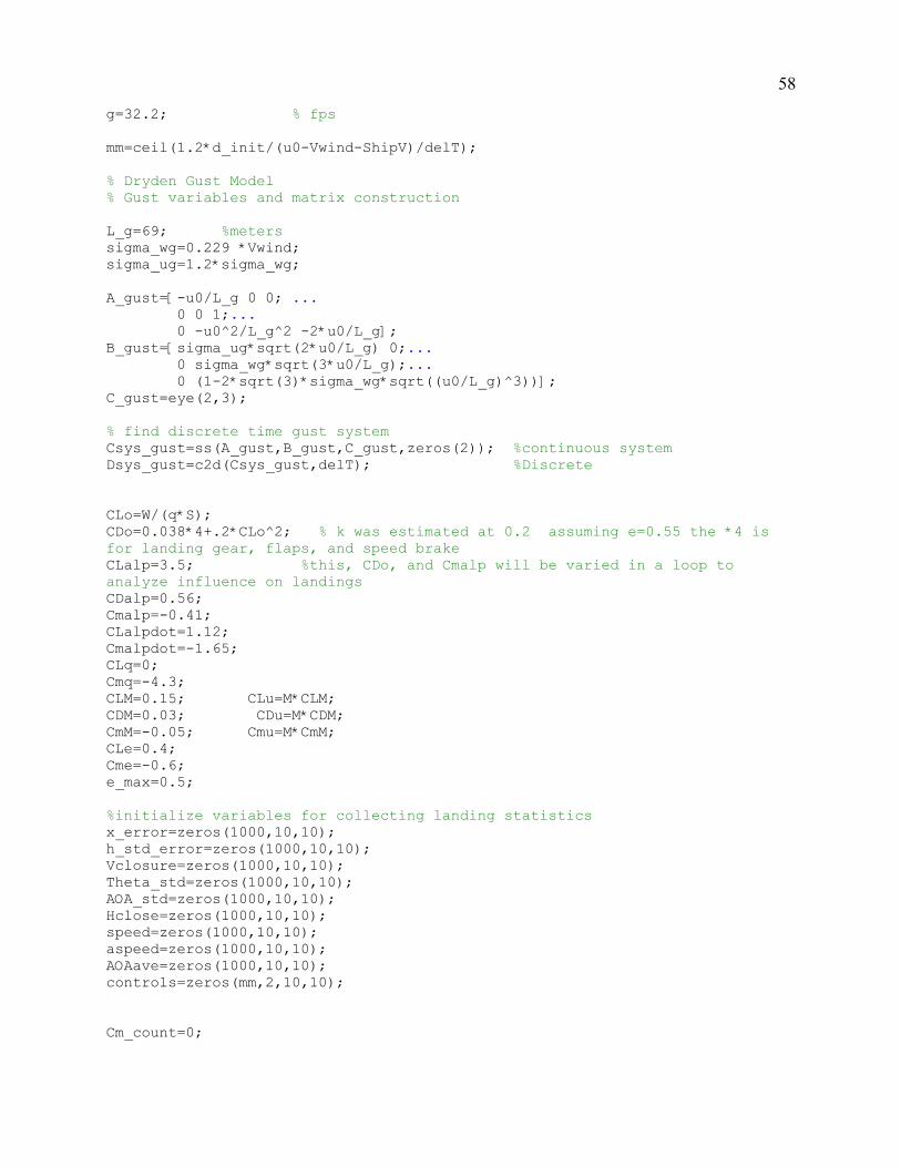
58
g=32.2; % fps mm=ceil(1.2*d_init/(u0-Vwind-ShipV)/delT); % Dryden Gust Model % Gust variables and matrix construction L_g=69; %meters sigma_wg=0.229 *Vwind; sigma_ug=1.2*sigma_wg; A_gust=[-u0/L_g 0 0; ... 0 0 1;... 0 -u0^2/L_g^2 -2*u0/L_g]; B_gust=[sigma_ug*sqrt(2*u0/L_g) 0;... 0 sigma_wg*sqrt(3*u0/L_g);... 0 (1-2*sqrt(3)*sigma_wg*sqrt((u0/L_g)^3))]; C_gust=eye(2,3); % find discrete time gust system Csys_gust=ss(A_gust,B_gust,C_gust,zeros(2)); %continuous system Dsys_gust=c2d(Csys_gust,delT); %Discrete CLo=W/(q*S); CDo=0.038*4+.2*CLo^2; % k was estimated at 0.2 assuming e=0.55 the *4 is for landing gear, flaps, and speed brake CLalp=3.5; %this, CDo, and Cmalp will be varied in a loop to analyze influence on landings CDalp=0.56; Cmalp=-0.41; CLalpdot=1.12; Cmalpdot=-1.65; CLq=0; Cmq=-4.3; CLM=0.15; CLu=M*CLM; CDM=0.03; CDu=M*CDM; CmM=-0.05; Cmu=M*CmM; CLe=0.4; Cme=-0.6; e_max=0.5; %initialize variables for collecting landing statistics x_error=zeros(1000,10,10); h_std_error=zeros(1000,10,10); Vclosure=zeros(1000,10,10); Theta_std=zeros(1000,10,10); AOA_std=zeros(1000,10,10); Hclose=zeros(1000,10,10); speed=zeros(1000,10,10); aspeed=zeros(1000,10,10); AOAave=zeros(1000,10,10); controls=zeros(mm,2,10,10); Cm_count=0;
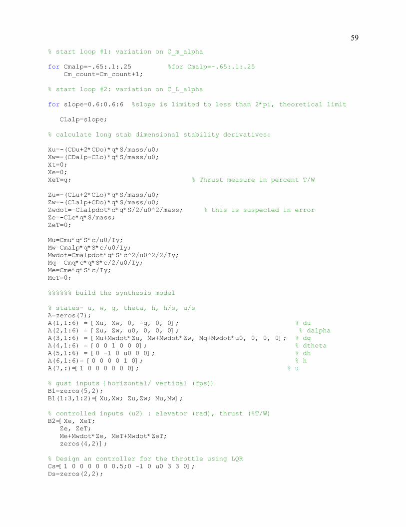
59
% start loop #1: variation on C_m_alpha for Cmalp=-.65:.1:.25 %for Cmalp=-.65:.1:.25 Cm_count=Cm_count+1; % start loop #2: variation on C_L_alpha for slope=0.6:0.6:6 %slope is limited to less than 2*pi, theoretical limit CLalp=slope; % calculate long stab dimensional stability derivatives: Xu=-(CDu+2*CDo)*q*S/mass/u0; Xw=-(CDalp-CLo)*q*S/mass/u0; Xt=0; Xe=0; XeT=g; % Thrust measure in percent T/W Zu=-(CLu+2*CLo)*q*S/mass/u0; Zw=-(CLalp+CDo)*q*S/mass/u0; Zwdot=-CLalpdot*c*q*S/2/u0^2/mass; % this is suspected in error Ze=-CLe*q*S/mass; ZeT=0; Mu=Cmu*q*S*c/u0/Iy; Mw=Cmalp*q*S*c/u0/Iy; Mwdot=Cmalpdot*q*S*c^2/u0^2/2/Iy; Mq= Cmq*c*q*S*c/2/u0/Iy; Me=Cme*q*S*c/Iy; MeT=0; %%%%%% build the synthesis model % states- u, w, q, theta, h, h/s, u/s A=zeros(7); A(1,1:6) = [Xu, Xw, 0, -g, 0, 0]; % du A(2,1:6) = [Zu, Zw, u0, 0, 0, 0]; % dalpha A(3,1:6) = [Mu+Mwdot*Zu, Mw+Mwdot*Zw, Mq+Mwdot*u0, 0, 0, 0]; % dq A(4,1:6) = [0 0 1 0 0 0]; % dtheta A(5,1:6) = [0 -1 0 u0 0 0]; % dh A(6,1:6)= [0 0 0 0 1 0]; % h A(7,:)=[1 0 0 0 0 0 0]; % u % gust inputs {horizontal/ vertical (fps)} B1=zeros(5,2); B1(1:3,1:2)=[Xu,Xw; Zu,Zw; Mu,Mw]; % controlled inputs (u2) : elevator (rad), thrust (%T/W) B2=[Xe, XeT; Ze, ZeT; Me+Mwdot*Ze, MeT+Mwdot*ZeT; zeros(4,2)]; % Design an controller for the throttle using LQR Cs=[1 0 0 0 0 0 0.5;0 -1 0 u0 3 3 0]; Ds=zeros(2,2);
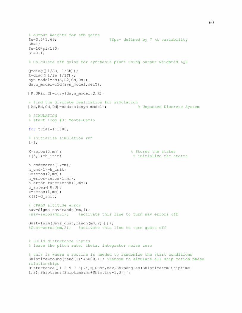
60
% output weights for sfb gains Su=3.5*1.69; %fps- defined by 7 kt variability Sh=1; Se=10*pi/180; ST=0.1; % Calculate sfb gains for synthesis plant using output weighted LQR Q=diag([1/Su, 1/Sh]); R=diag([1/Se 1/ST]); syn_model=ss(A,B2,Cs,Ds); dsyn_model=c2d(syn_model,delT); [K,SRic,E]=lqry(dsyn_model,Q,R); % find the discrete realization for simulation [Ad,Bd,Cd,Dd]=ssdata(dsyn_model); % Unpacked Discrete System % SIMULATION % start loop #3: Monte-Carlo for trial=1:1000, % Initialize simulation run i=1; X=zeros(5,mm); % Stores the states X(5,1)=h_init; % initialize the states h_cmd=zeros(1,mm); h_cmd(1)=h_init; u=zeros(2,mm); h_error=zeros(1,mm); h_error_rate=zeros(1,mm); u_integ=[0;0]; x=zeros(1,mm); x(1)=d_init; % JPALS altitude error nav=Sigma_nav*randn(mm,1); %nav=zeros(mm,1); %activate this line to turn nav errors off Gust=lsim(Dsys_gust,randn(mm,2),[]); %Gust=zeros(mm,2); %activate this line to turn gusts off % Build disturbance inputs % leave the pitch rate, theta, integrator noise zero % this is where a routine is needed to randomize the start conditions Shiptime=round(rand(1)*45000)+1; %random to simulate all ship motion phase relationships Disturbance([1 2 5 7 8],:)=[Gust,nav,ShipAngles(Shiptime:mm+Shiptime-1,2),Shiptrans(Shiptime:mm+Shiptime-1,3)]';
61
% start loop #4: time step simulation while X(5,i) >=(13.62-(x(i)+Shiptrans(i+Shiptime-1,1)-ShipH*Disturbance(7,i))*Disturbance(7,i)-Disturbance(8,i)), % accounts for ship pitch, surge, and heave i=i+1; if i==mm % safety condition to prevent falling into infinite loop warning('i=mm flying slow') x(i) avespeed=sum(X(1,:))/i break end % calculate the lateral distance from the origin (integrate velocity) x(i)=x(i-1)-(u0-ShipV-Vwind+X(1,i-1))*delT; % u0-ShipV-Vwind+X(1,i-1)=closing velocity % h_cmd is the sum of the glideslope, and its time varying ship motion h_cmd(i)=x(i)*tGlide+ship(i+Shiptime-1); % simulation step (5 more integrations here) % dynamics control inputs 2-dim gust X(:,i)=Ad(1:5,1:5)*X(:,i-1)+ Bd(1:5,:)*u(:,i-1)+ delT*B1(:,1:2)*Disturbance(1:2,i); % calculate true altitude error h_error(i)=X(5,i)-h_cmd(i); % calculate altitude error rate % acft sink rate ship rate glideslope bias h_error_rate(i)=A(5,1:4)*X(1:4,i)-(shiprate(i+Shiptime-1)-(u0-ShipV-Vwind+X(1,i-1))*tGlide); % integral action within the controller
u_integ= u_integ + delT*K(:,5:7)*[h_error_rate(i); h_error(i)+nav(i);X(1,i)];
% calculate elevator and throttle command for next time step u(:,i)= -K(:,1:4)*X(1:4,i) - u_integ; end % loop #4 % collect statistic for simulation run bb=round(i/8); % start here to chop off start-up errors X=X(:,bb:i); h_cmd=h_cmd(bb:i); hdot=A(5,1:4)*X(1:4,:); x=x(bb:i); u=u(:,bb:i); h_error=h_error(:,bb:i); Disturbance=Disturbance(:,bb:i); Gust=Gust(bb:i,:); L=length(h_error); count_sl=round(slope/.6); z1=X(5,L-1)-(13.62-(x(L-1)-ShipH*Disturbance(7,L-1))*Disturbance(7,L-1)-Disturbance(8,L-1));
62
z2=X(5,L)-(13.62-(x(L)-ShipH*Disturbance(7,L))*Disturbance(7,L)-Disturbance(8,L)); xland=(x(L-1)-x(L))*z1/(z1-z2)+x(L-1); x_error(trial,count_sl,Cm_count)=ShipL-xland; %positive error means landing was long % error stats [h_error @LA, average h_error,theta_perterbation,aoa_perterbation,vert closure, h_dot,x_dot] h_std_error(trial,count_sl,Cm_count)= std(h_error); %standard deviation of altitude error during flight % vertical rate ignores: true landing distance (this would be easy to adopt), % and heave rate (negligible) Vclosure(trial,count_sl,Cm_count)=shiprate(i+Shiptime-1)-hdot(L); Hclose(trial,count_sl,Cm_count)=X(1,L)+u0-ShipV-Vwind; aspeed(trial,count_sl,Cm_count)=sum(X(1,:))/L; Theta_std(trial,count_sl,Cm_count)=std(X(4,:)-sum(X(4,:)/L)); AOA_std(trial,count_sl,Cm_count)=std(X(2,:))/(u0+aspeed(trial,count_sl,Cm_count)); AOAave(trial,count_sl,Cm_count)=sum(X(2,:)/L)/(u0+aspeed(trial,count_sl,Cm_count)); speed(trial,count_sl,Cm_count)=std(X(1,:)); Disturbance=zeros(8,mm); end %end trial loop (loop #3) controls(1:L,:,count_sl,Cm_count)=u'; controls(mm,:,count_sl,Cm_count)=L; save Lnd_StatN12 x_error h_std_error Vclosure Hclose Theta_std AOA_std configuration speed aspeed AOAave controls end % end loop changing Clalp (loop #2) Cm_count end %end loop for Cmalp (loop #1)

63
APPENDIX II : PLAN OF ACTION AND MILESTONES
Due Status Task Action 19-Aug Fall Semester Classes Begin
done JPALS signal analysis for frequency content Sweger done Basic longitudinal glide slope tracking model Sweger
2-Sep Holiday -- Labor Day done Define ship motion influences on the landing area Sweger
13 -15 Sept 1/C Parents Weekend
done Write a section on the ship motion and equations Sweger done Write a section on JPALS model Sweger
14-Oct Holiday -- Columbus Day done Integrate ship motion into flight model Sweger done Build gust model Sweger done Integrate gust model Sweger done Write section on gust model Sweger
11-Nov Holiday -- Veteran's Day done Define synthesis model for H-infinity controller Sweger/Niewoehner done Write section on manned vs. unmanned issues Sweger Debug H-infinity controller Niewoehner done Write section on the over all model Sweger
28-Nov Holiday -- Thanksgiving done Compile sections for interim report Sweger Revise interim report Sweger
4-Dec NLT NOON: Submit, via e-mail, POA&M to Dean Miller ("cc" adviser and DDRS)
4-Dec NLT 1400: Submission of Interim Trident Scholar Reports to DDRS

64
Begin building lateral mode simulation model Sweger 6-Dec End of Fall Semester Classes
Build a data collection structure for the sensitivity analysis Sweger Begin sensitivity analysis on longitudinal mode Sweger
10-Dec - 3-Jan End of Semester Leave
Due Status Task Action 7-Jan Spring Semester Classes Begin
Continue attempts to incorporate lead compensation Hallberg/Niewoehner
20-Jan Holiday -- Martin Luther King Day Control structure fixed Hallberg/Niewoehner
17-Feb Holiday -- President's Day Run simulations for sensitivity analysis Sweger Restrict study to longitudinal characteristics only due to time constraints
7-Mar - 16-Mar SPRING BREAK
Compile longitudinal simulation results from sensitivity analysis Sweger
Anaylze the sensitivity to lift curve slope and elevator power Sweger Anaylze the sensitivity to throttle lag and moment of inertia Sweger Anaylze sensitivity to sea-state and wind-over-deck Sweger Begin preparing final presentation Sweger Prepare results graphics for report Sweger Run simulations to fill gaps discovered during the writing phase Sweger Write draft criteria Sweger Continue working on final report Sweger Proof read report Niewoehner Revise presentation, practice presenting Sweger
18-Apr Submission of "Cmte-Ready" Versions of Trident Scholar Reports to DDRS
24-Apr Day 1: Trident Scholar Conference 25-Apr Day 2: Trident Scholar Conference

65
26-Apr Trident Scholar Poster Session and Banquet 29-Apr End of Spring Semester Classes
Finish revising final report Sweger
5-May Submission of Final Versions of Trident Scholar Reports to DDRS
23-May Graduation Class of 2003
66
APPENDIX III : SHIP MOTION SIMULATION CODE % ************************************************************************* % CVN65dynamics CVN 65 motion constants generated from SMP program, NSRDC % (David Taylor). Ship speed = 15 knots, 30 deg relative to % long crested waves, wave period = 15 sec. % % Sea State Wave Height % 3 8.2 ft % 4 13.1 ft % 5 19.7 ft. % % Raw amplitudes correspond to 2*RMS but are scaled for 3*RMS using "kmot". % Therefore, maximum amplitudes of motion are simulated. % % ************************************************************************* % $Header: \\\\Uavlabnt1\\UAVLab\040Share\\Projects\\CVS_ROOT/F18_JPALS/F18Sim/CVN65dynamics.m,v 1.3 2001/01/05 17:06:13 AksteterJW Exp $ % ************************************************************************* % Changes: % % $Log: CVN65dynamics.m,v $ % Revision 1.3 2001/01/05 17:06:13 AksteterJW % Slight documentation mod. for clarification. Also, % some spec. disturbance frequencies under each sea state were equivalent. % So some frequencies were adjusted rel. to their spec. values so that they % differ by >= 0.05 rad/sec relative to one another. This gives dissimilar % beat frequencies, hence more statistically meaningful simulations. The % spec. values were added in parentheses to the right for reference. % % Revision 1.2 2000/12/05 19:17:41 AksteterJW % Documentation including input and output parameter definitions. % % % ************************************************************************* % Inputs %************************************************************************** % iseastate Sea state value (e.g., 3, 4, or 5) % iship Switch for oscillatory ship motion (sway,heave,etc.)[0=off;1=on] % %************************************************************************** % Outputs %************************************************************************** % surgeamp Amplitude of ships surge motion (ft) % surgefreq Frequency of ships surge motion (rad/sec) % yawamp Amplitude of ships yaw motion (deg) % yawfreq Frequency of ships yaw motion (rad/sec) % swayamp Amplitude of ships sway motion (ft) % swayfreq Frequency of ships sway motion (rad/sec) % heaveamp Amplitude of ships heave motion (ft) % heavefreq Frequency of ships heave motion (rad/sec) % pitchamp Amplitude of ships pitch motion (deg) % pitchfreq Frequency of ships pitch motion (rad/sec) % rollamp Amplitude of ships roll motion (deg)
67
% rollfreq Frequency of ships roll motion (rad/sec) %************************************************************************** if iseastate==3 % if iseastate==3 % ************************************************************************* % SHIP MOTION CONSTANTS (3*RMS) % CVN 65 Sea State 3 % ************************************************************************ kmot=1.5; %Motion Scaling iiship=kmot*iship; % The following ship motions are driven by sine waves surgeamp = 0.8*iiship; % Amplitude of ships surge motion (ft) surgefreq = 0.35; % (0.45) Frequency of ships surge motion (rad/sec) yawamp = 0.12*iiship; % Amplitude of ships yaw motion (deg) yawfreq = 0.63; % (0.63) Frequency of ships yaw motion (rad/sec) swayamp = 0.53*iiship; % Amplitude of ships sway motion (ft) swayfreq = 0.45; % (0.45) Frequency of ships sway motion (rad/sec) heaveamp = 1.99*iiship; % Amplitude of ships heave motion (ft) heavefreq = 0.53; % (0.48) Frequency of ships heave motion (rad/sec) pitchamp = 0.72*iiship; % Amplitude of ships pitch motion (deg) pitchfreq = 0.58; % (0.57) Frequency of ships pitch motion (rad/sec) rollamp = 0.21*iiship; % Amplitude of ships roll motion (deg) rollfreq = 0.40; % (0.57) Frequency of ships roll motion (rad/sec) elseif iseastate==4 % ************************************************************************* % SHIP MOTION CONSTANTS (3*RMS) % CVN 65 Sea State 4 % *********************************************************************** kmot=1.5; %Motion Scaling iiship=kmot*iship; % The following ship motions are driven by sine waves surgeamp = 1.32*iiship; % Amplitude of ships surge motion (ft) surgefreq = 0.35; % (0.45) Frequency of ships surge motion (rad/sec) yawamp = 0.30*iiship; % Amplitude of ships yaw motion (deg) yawfreq = 0.50; % (0.52) Frequency of ships yaw motion (rad/sec) swayamp = 0.84*iiship; % Amplitude of ships sway motion (ft) swayfreq = 0.40; % (0.45) Frequency of ships sway motion (rad/sec) heaveamp = 3.59*iiship; % Amplitude of ships heave motion (ft)
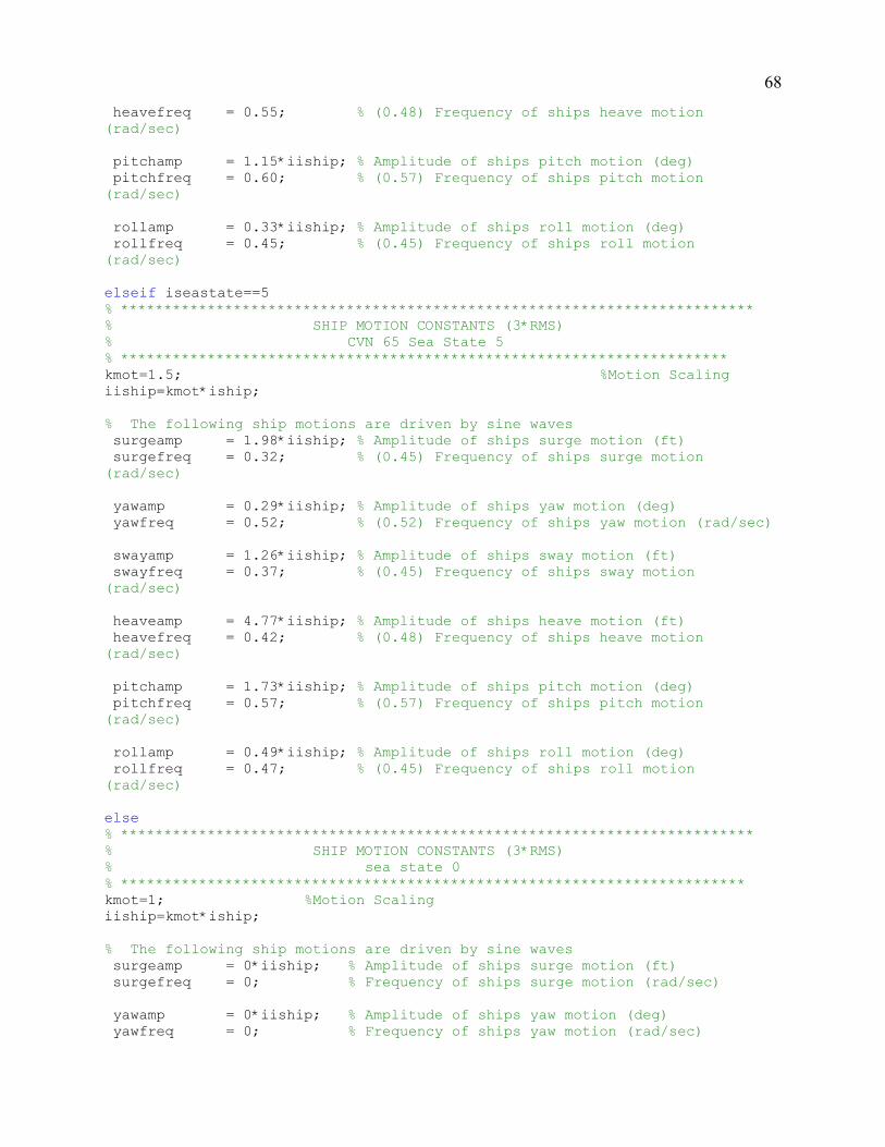
68
heavefreq = 0.55; % (0.48) Frequency of ships heave motion (rad/sec) pitchamp = 1.15*iiship; % Amplitude of ships pitch motion (deg) pitchfreq = 0.60; % (0.57) Frequency of ships pitch motion (rad/sec) rollamp = 0.33*iiship; % Amplitude of ships roll motion (deg) rollfreq = 0.45; % (0.45) Frequency of ships roll motion (rad/sec) elseif iseastate==5 % ************************************************************************* % SHIP MOTION CONSTANTS (3*RMS) % CVN 65 Sea State 5 % ********************************************************************** kmot=1.5; %Motion Scaling iiship=kmot*iship; % The following ship motions are driven by sine waves surgeamp = 1.98*iiship; % Amplitude of ships surge motion (ft) surgefreq = 0.32; % (0.45) Frequency of ships surge motion (rad/sec) yawamp = 0.29*iiship; % Amplitude of ships yaw motion (deg) yawfreq = 0.52; % (0.52) Frequency of ships yaw motion (rad/sec) swayamp = 1.26*iiship; % Amplitude of ships sway motion (ft) swayfreq = 0.37; % (0.45) Frequency of ships sway motion (rad/sec) heaveamp = 4.77*iiship; % Amplitude of ships heave motion (ft) heavefreq = 0.42; % (0.48) Frequency of ships heave motion (rad/sec) pitchamp = 1.73*iiship; % Amplitude of ships pitch motion (deg) pitchfreq = 0.57; % (0.57) Frequency of ships pitch motion (rad/sec) rollamp = 0.49*iiship; % Amplitude of ships roll motion (deg) rollfreq = 0.47; % (0.45) Frequency of ships roll motion (rad/sec) else % ************************************************************************* % SHIP MOTION CONSTANTS (3*RMS) % sea state 0 % ************************************************************************ kmot=1; %Motion Scaling iiship=kmot*iship; % The following ship motions are driven by sine waves surgeamp = 0*iiship; % Amplitude of ships surge motion (ft) surgefreq = 0; % Frequency of ships surge motion (rad/sec) yawamp = 0*iiship; % Amplitude of ships yaw motion (deg) yawfreq = 0; % Frequency of ships yaw motion (rad/sec)
69
swayamp = 0*iiship; % Amplitude of ships sway motion (ft) swayfreq = 0; % Frequency of ships sway motion (rad/sec) heaveamp = 0*iiship; % Amplitude of ships heave motion (ft) 6.0 heavefreq = 0; % Frequency of ships heave motion (rad/sec) pitchamp = 0*iiship; % Amplitude of ships pitch motion (deg) 1.6 pitchfreq = 0; % Frequency of ships pitch motion (rad/sec) rollamp = 0*iiship; % Amplitude of ships roll motion (deg) rollfreq = 0; % Frequency of ships roll motion (rad/sec) end % END if iseastate==3 function IJK=geod2ecef(lat,lon,alt) % function IJK=geod2ecef(lat,lon,alt) % Convert Earth Centered Earth Fixed (ECEF) Cartesian coordinates % to Geodetic coordinates % inputs: % lat - Geodetic Latitude (deg) % lon - Geodetic Longitude (deg) % alt - Geodetic Altitude (ft); % outputs: % x Equatorial Prime meridian coordinate (ft) % y Equatoral 90 deg Long. coordinate (ft) % z North coordinate (ft) % uses WGS-84 Ellipsoidal Model. % %%%%%%%%%%%%%%%%%%%%%%%%%%%%%%%%%%%%%%%%%%%%%%%%%%%% % 6/14/99 % Eric Schug (SAIC) %%%%%%%%%%%%%%%%%%%%%%%%%%%%%%%%%%%%%%%%%%%%%%%%%%%% % $Header: \\\\Uavlabnt1\\UAVLab\040Share\\Projects\\CVS_ROOT/F18_JPALS/F18Sim/geod2ecef.m,v 1.2 2002/05/29 15:15:11 SchugEC Exp $ % Changes % $Log: geod2ecef.m,v $ % Revision 1.2 2002/05/29 15:15:11 SchugEC % Restoring Lastest F18_JPALS after deleting CVS files % % Revision 1.3 2002/03/22 21:47:39 SchugEC % vectorized it % % Revision 1.2 2001/12/12 20:46:27 AksteterJW % Header documentation. % % Revision 1.1 2000/10/26 18:39:53 SchugEC % Initial addtions % %%%%%%%%%%%%%%%%%%%%%%%%%%%%%%%%%%%%%%%%%%%%%%%%%%%% %%%%%%%%%%%%%%%%%%%%%%%%%%%%%%%%%%%%%%%%%%%%%%%%%%%%%%%
70
% Constants Originally in MKS units, converted to ft,sec %%%%%%%%%%%%%%%%%%%%%%%%%%%%%%%%%%%%%%%%%%%%%%%%%%%%%% m2ft = 3.28083989501312; a = 6378137.0*m2ft; % semi-major axis e2 = 6.69437999014e-3; % First Eccentricity Squared ELIN = 5.2185400842339e5*m2ft; % Linear Eccentricity E2 = ELIN*ELIN; b_a=0.996647189335; % major/minor axis ratio lat=lat*pi/180; lon=lon*pi/180; fslat=sqrt(1-e2*sin(lat).^2); Rp=a./fslat; IJK(:,1)=(Rp+alt).*cos(lat).*cos(lon); IJK(:,2)=(Rp+alt).*cos(lat).*sin(lon); IJK(:,3)=(Rp.*b_a.^2+alt).*sin(lat); % load_ship kts2fps = 1.6878; fps2kts = 1/kts2fps; %*********************************************** % You can adjust these ShipCMlat = 0; ShipCMlon = 0; iseastate = 3; tend = 10; spi = 10*kts2fps; % ship speed in ft/sec turntime = 5; % time when ship turn starts (sec) turndeg = 0; % desired ship turn angle (deg) psiski = 0; % initial ship heading (deg) %*********************************************** ishpmotion = 'CVN65'; iship = 1; % 1=ON, 0=OFF dt = 0.01; nsave = 1; numpts = inf; d2r = pi/180; fprintf('Ship CM Latitude = %7.2f (deg) \n',ShipCMlat) fprintf('Ship CM Longitude = %7.2f (deg) \n',ShipCMlon) fprintf('Ship Motion: %-9.9s Sea State %2d \n', ishpmotion,iseastate) fprintf('Simulation run time = %7.2f (sec) \n',tend) fprintf('Ship Velocity =%8.2f kts\n',spi*fps2kts) ShipCMecef=geod2ecef(ShipCMlat,ShipCMlon,0); CVN65dynamics seedsize = max(1,1); rand('seed',999) delphase=2*pi*rand(6,seedsize); % repeatable phase set for ionce = 1==>maxautorun
71
surgephase = delphase(1,1); % Initial phase of surge motion (rad) yawphase = delphase(2,1); % Initial phase of yaw motion (rad) swayphase = delphase(3,1); % Initial phase of sway motion (rad) heavephase = delphase(4,1); % Initial phase of heave motion (rad) pitchphase = delphase(5,1); % Initial phase of pitch motion (rad) rollphase = delphase(6,1); % Initial phase of roll motion (rad) % ************************************************************ % Initial ship Euler rates (local frame) % ************************************************************ psid_0=(yawamp*yawfreq*cos(yawphase))*d2r; % Heading rate, rad/s (+cwn) thed_0=(pitchamp*pitchfreq*cos(pitchphase))*d2r; % Pitch rate, rad/s (+bow up) phid_0=(rollamp*rollfreq*cos(rollphase))*d2r; % Roll rate, rad/s (+stbd dn) % ************************************************************************* % Call the SIMULINK simulation % ************************************************************************* % Simulation Setup tol = 1e-4; minstep = dt; maxstep = dt; tfinal = tend; simstruct=simset('Solver','ode1','FixedStep',dt,'OutputVariables','t',... 'Decimation',nsave,'RelTol',tol); [time]=sim('ship',tfinal,simstruct);