Embed Size (px)
Citation preview

Design, Simulation, and Wind Tunnel Verification of a MorphingAirfoil
Eric A. Gustafson
Thesis submitted to the Faculty of theVirginia Polytechnic Institute and State University
in partial fulfillment of the requirements for the degree of
Master of Sciencein
Mechanical Engineering
Kevin B. Kochersberger, ChairDaniel J. Inman
Robert A. Canfield
May 25, 2011Blacksburg, Virginia
Keywords: Morphing, Macro Fiber Composite, Thin Cambered Airfoil, GenMAVCopyright 2011, Eric A. Gustafson

Design, Simulation, and Wind Tunnel Verification of a Morphing Airfoil
Eric A. Gustafson
ABSTRACT
The application of smart materials to control the flight dynamics of a Micro Air Vehicle(MAV) has numerous benefits over traditional servomechanisms. Under study is wing mor-phing achieved through the use of piezoelectric Macro Fiber Composites (MFCs). Thesedevices exhibit low power draw but excellent bandwidth characteristics. This thesis providesa background in the 2D analytical and computer modeling tools and methods needed todesign and characterize an MFC-actuated airfoil.
A composite airfoil is designed with embedded MFCs in a bimorph configuration. The deflec-tion capabilities under actuation are predicted with the commercial finite element packageNX Nastran. Placement of the piezoelectric actuator is studied for optimal effectiveness. Athermal analogy is used to represent piezoelectric strain. Lift and drag coefficients in lowReynolds number flow are explored with XFOIL. Predictions are made on static aeroelasticeffects. The thin, cambered Generic Micro Aerial Vehicle (GenMAV) airfoil is fabricatedwith a bimorph actuator. Experimental data are taken with and without aerodynamic load-ing to validate the computer model. This is accomplished with in-house 2D wind tunneltesting.

To my parents David and Beverly Gustafson
iii

Acknowledgments
I would like to acknowledge and thank the crews of old and new at the VT Unmanned SystemsLab, especially (in no order) Mike Rose, Jimmy May, Kevin Stefanik, Kenny Kroeger, JerryTowler, Brian McCabe, and Shajan Thomas. I would be remiss to not thank Dr. KevinKochersberger for offering me this opportunity, and for being the reason this project wasable to take foot. I’d like to extend my gratitude to Dr. Canfield for his valuable input on mythesis and research. A special thanks goes out to my parents, David and Beverly Gustafson,and my siblings, Stephen and Darla, for their support at every point of my progress.
I appreciate the efforts of AVID LLC, and especially John Ohanian, for their guidance duringthe project. As with all research, this work represents an extension on the academic pursuitsof others, and for that I thank Dr. Onur Bilgen. Additionally, I’d like to acknowledge theVT CIMSS lab for granting me use of their wind tunnel which enabled the latter half of thisresearch.
This work was produced in collaboration with AVID LLC as part of a Phase I and II SBIRfrom the US Air Force Research Laboratory (AFRL), Eglin, FL.
iv

Contents
1 Introduction 11.1 Background . . . . . . . . . . . . . . . . . . . . . . . . . . . . . . . . . . . . 11.2 Motivation . . . . . . . . . . . . . . . . . . . . . . . . . . . . . . . . . . . . . 4
2 Literature Review 52.1 Active Wing Structures . . . . . . . . . . . . . . . . . . . . . . . . . . . . . . 6
2.1.1 Maneuverability Morphing . . . . . . . . . . . . . . . . . . . . . . . . 62.1.2 Configuration Morphing . . . . . . . . . . . . . . . . . . . . . . . . . 8
2.2 Finite Element Modeling of Piezoelectrics . . . . . . . . . . . . . . . . . . . . 9
3 Mechanical Simulation with FEA 113.1 Airfoil Selection . . . . . . . . . . . . . . . . . . . . . . . . . . . . . . . . . . 113.2 Macro Fiber Composites Properties . . . . . . . . . . . . . . . . . . . . . . . 123.3 Composite Substrates . . . . . . . . . . . . . . . . . . . . . . . . . . . . . . . 133.4 Thermal Analogy . . . . . . . . . . . . . . . . . . . . . . . . . . . . . . . . . 183.5 Finite Element Modeling of Piezoelectric Strain . . . . . . . . . . . . . . . . 20
3.5.1 Application of Thermal Analogy . . . . . . . . . . . . . . . . . . . . . 203.5.2 Bare MFC . . . . . . . . . . . . . . . . . . . . . . . . . . . . . . . . . 223.5.3 Bimorph Actuator . . . . . . . . . . . . . . . . . . . . . . . . . . . . 233.5.4 GenMAV . . . . . . . . . . . . . . . . . . . . . . . . . . . . . . . . . 25
4 MFC Driver Electronics 314.1 Lightweight Circuit Prototype . . . . . . . . . . . . . . . . . . . . . . . . . . 31
4.1.1 Lightweight Circuit Schematic . . . . . . . . . . . . . . . . . . . . . . 324.1.2 Flight Weight PCB Design . . . . . . . . . . . . . . . . . . . . . . . . 34
4.2 Experimentation Circuit . . . . . . . . . . . . . . . . . . . . . . . . . . . . . 36
5 Static Actuation Testing 375.1 Experimental Setup . . . . . . . . . . . . . . . . . . . . . . . . . . . . . . . . 375.2 Model Fabrication . . . . . . . . . . . . . . . . . . . . . . . . . . . . . . . . . 395.3 Model Comparison . . . . . . . . . . . . . . . . . . . . . . . . . . . . . . . . 40
6 Aerodynamic Analysis 43
v

6.1 XFOIL . . . . . . . . . . . . . . . . . . . . . . . . . . . . . . . . . . . . . . . 436.2 GenMAV . . . . . . . . . . . . . . . . . . . . . . . . . . . . . . . . . . . . . 436.3 Cp Distributions . . . . . . . . . . . . . . . . . . . . . . . . . . . . . . . . . . 456.4 Refinement of Airfoil Design . . . . . . . . . . . . . . . . . . . . . . . . . . . 476.5 Sectional Cd, Cl Predictions . . . . . . . . . . . . . . . . . . . . . . . . . . . 486.6 Static Aeroelastic Response . . . . . . . . . . . . . . . . . . . . . . . . . . . 49
7 Wind Tunnel Testing 547.1 Wind Tunnel Facility and Instrumentation . . . . . . . . . . . . . . . . . . . 547.2 2D Lift & Drag Coefficients . . . . . . . . . . . . . . . . . . . . . . . . . . . 577.3 Model Fabrication and Installation . . . . . . . . . . . . . . . . . . . . . . . 587.4 Reference Airfoil Investigation . . . . . . . . . . . . . . . . . . . . . . . . . . 597.5 Experimental Procedure . . . . . . . . . . . . . . . . . . . . . . . . . . . . . 607.6 Results . . . . . . . . . . . . . . . . . . . . . . . . . . . . . . . . . . . . . . . 61
7.6.1 Sectional Cd and Cl Results . . . . . . . . . . . . . . . . . . . . . . . 627.6.2 Measurement Uncertainty . . . . . . . . . . . . . . . . . . . . . . . . 667.6.3 Model Comparison . . . . . . . . . . . . . . . . . . . . . . . . . . . . 697.6.4 Limit Cycle Oscillations . . . . . . . . . . . . . . . . . . . . . . . . . 70
8 Conclusion 748.1 Summary . . . . . . . . . . . . . . . . . . . . . . . . . . . . . . . . . . . . . 748.2 Recommendations of Future Work . . . . . . . . . . . . . . . . . . . . . . . . 76
Bibliography 77
A Generating Laminate Stiffness Properties 81A.1 Micromechanics . . . . . . . . . . . . . . . . . . . . . . . . . . . . . . . . . . 82A.2 Ply Mechanics . . . . . . . . . . . . . . . . . . . . . . . . . . . . . . . . . . . 83A.3 Macromechanics . . . . . . . . . . . . . . . . . . . . . . . . . . . . . . . . . . 84
B MATLAB Code for Determining Sensitivity of Laminate Mechanical Prop-erties to Substrate Orientation 87
C Composite Layup Process 91C.1 Notes on Composite Fabrics and Suppliers . . . . . . . . . . . . . . . . . . . 93
D GenMAV Airfoil Coordinates 94
E Additional Wind Tunnel Testing Details 95E.1 Lift & Drag Coefficient Corrections . . . . . . . . . . . . . . . . . . . . . . . 95E.2 Load Cell Calibrations . . . . . . . . . . . . . . . . . . . . . . . . . . . . . . 97E.3 Variation of WT Flow Speeds . . . . . . . . . . . . . . . . . . . . . . . . . . 98E.4 LCO Amplitude and Frequency Plots . . . . . . . . . . . . . . . . . . . . . . 99E.5 Laser Displacement Plots . . . . . . . . . . . . . . . . . . . . . . . . . . . . . 102
vi

F Additional Lightweight Circuit Details 104
vii

List of Figures
1.1 The M4010-P1 MFC actuator. . . . . . . . . . . . . . . . . . . . . . . . . . . 21.2 Exploded view of all layers comprising a generic MFC actuator. . . . . . . . 2
3.1 The GenMAV airfoil shape. . . . . . . . . . . . . . . . . . . . . . . . . . . . 123.2 Reference directions for thermal analogy with respect to the alignment of
electrodes. . . . . . . . . . . . . . . . . . . . . . . . . . . . . . . . . . . . . . 123.3 Illustration of laminate coordinate system with respect to fiber directions. . . 143.4 Variation of in-plane elastic moduli Eb
x & Eby for a woven ply of various materials 16
3.5 Variation of shear modulus Gbxy and in-plane Poisson’s ratio νbxy for a woven
ply of various materials. . . . . . . . . . . . . . . . . . . . . . . . . . . . . . 173.6 Bare MFC actuator with one fixed node and temperature-only loading. . . . 223.7 Bare MFC deformed and undeformed shapes. . . . . . . . . . . . . . . . . . 233.8 Predicted bimorph displacements from nonlinear solver. . . . . . . . . . . . . 243.9 Raised side view of GenMAV airfoil. . . . . . . . . . . . . . . . . . . . . . . 253.10 The finite element model showing placement of temperature loads and con-
straints. . . . . . . . . . . . . . . . . . . . . . . . . . . . . . . . . . . . . . . 263.11 Side view of the embedded bimorph actuator. . . . . . . . . . . . . . . . . . 273.12 Maximum static deflection of the airfoil for actuator placement at various
chordwise stations. . . . . . . . . . . . . . . . . . . . . . . . . . . . . . . . . 283.13 Maximum static deflection of the airfoil for various substrate orientation and
thicknesses. . . . . . . . . . . . . . . . . . . . . . . . . . . . . . . . . . . . . 293.14 Maximum static deflection of the airfoil for various materials and thicknesses. 30
4.1 Electrical schematic of the lightweight MFC driver PCB. . . . . . . . . . . . 324.2 The output voltages of the two variable output converters over the actuation
range. . . . . . . . . . . . . . . . . . . . . . . . . . . . . . . . . . . . . . . . 334.3 Top and bottom layers of the lightweight MFC driver PCB. . . . . . . . . . . 354.4 Asymmtetric voltage divider concept schematic. . . . . . . . . . . . . . . . . 36
5.1 Experimental setup used to gauge bimorph shape under actuation for staticdeflection tests. . . . . . . . . . . . . . . . . . . . . . . . . . . . . . . . . . . 38
5.2 Bimorph mount and laser displacement sensor used for static deflection tests. 385.3 Voltage input and expected outputs two MFCs in a bimorph configuration. . 395.4 The zero camber bimorph used for model comparisons. . . . . . . . . . . . . 40
viii
5.5 Bimorph deflection results of four tests under identical conditions but differenttimes. . . . . . . . . . . . . . . . . . . . . . . . . . . . . . . . . . . . . . . . 41
5.6 Hysteresis demonstrated during an actuation/voltage sweep 0%→ −100%→+100%→ −100%→ 0%. . . . . . . . . . . . . . . . . . . . . . . . . . . . . . 42
6.1 XFOIL panel distribution from raw coordinates import. . . . . . . . . . . . . 446.2 Refined geometry for importing coordinates into XFOIL. . . . . . . . . . . . 446.3 Conditioned GenMAV airfoil coordinates for importing into XFOIL. . . . . . 456.4 Distribution and vector plot of the Cp distribution on the GenMAV airfoil. . 466.5 Maximum static deflection of the LE for various thicknesses. . . . . . . . . . 476.6 Baseline lift polar and drag data for the GenMAV as given by XFOIL. . . . 486.7 Baseline lift/Drag ratio versus angle of attack for the GenMAV airfoil. . . . . 496.8 Numerical procedure for obtaining convergence of static aeroelastic predictions. 516.9 The pattern of displacements at 45% input after pressure loading is applied. 526.10 Convergence trends of the airfoil deflections at 45% input through the iterations. 526.11 The pattern of displacements at 90% input after pressure loading is applied. 53
7.1 The open loop WT setup with the inlet in the foreground. . . . . . . . . . . 557.2 Layout of the CIMSS wind tunnel. Figure not to scale. . . . . . . . . . . . . 567.3 The airfoil with embedded M8557-P1 actuator. . . . . . . . . . . . . . . . . . 587.4 Airfoil mounted in the wind tunnel. . . . . . . . . . . . . . . . . . . . . . . . 597.5 Comparison of lift and drag results for the NACA 0009 airfoil. . . . . . . . . 607.6 Airfoil deflections in the wind tunnel under aero loading. . . . . . . . . . . . 617.7 Lift versus angle of attack for the morphing GenMAV airfoil at U = 9m/s . 627.8 Lift versus angle of attack for the morphing GenMAV airfoil at U = 13m/s . 627.9 Lift versus angle of attack for the morphing GenMAV airfoil at U = 17m/s . 637.10 Cl,max versus actuation for the morphing GenMAV airfoil at U = 9, 13, 17m/s 647.11 Drag versus angle of attack for the morphing GenMAV airfoil at U = 9, 13, 17m/s 657.12 Lift/ drag coefficient uncertainty as a function of test setting. . . . . . . . . 677.13 Cl predictions versus actuation at U = 9m/s and α = 0. . . . . . . . . . . . 697.14 Frequency response of trailing edge displacements for indicated flow speeds
and α = 15 . . . . . . . . . . . . . . . . . . . . . . . . . . . . . . . . . . . . 727.15 RMS amplitude response of trailing edge displacements for indicated flow
speeds and α = 15 . . . . . . . . . . . . . . . . . . . . . . . . . . . . . . . . 73
A.1 Steps taken to generate mechanical properties of composite substrates. . . . 82
C.1 Creating the mold for the GenMAV airfoil. . . . . . . . . . . . . . . . . . . . 92
E.1 Load cell output as a function of output voltage. . . . . . . . . . . . . . . . . 97E.2 Standard deviation of flow speed measurements as a function of flow speed. . 98E.3 Average wind tunnel speeds towards the lower limit of the flow speed range. 98E.4 Average wind tunnel speeds around the middle of the flow speed range. . . . 99E.5 Static displacements versus input voltage for flow speeds U = 9, 13, 17m/s. . 103
ix

F.1 Electrical schematic of the lightweight MFC driver PCB. . . . . . . . . . . . 105F.2 Final populated revision 1 of the lightweight circuit prototype. . . . . . . . . 105
x

List of Tables
3.1 Orthotropic properties of the MFC actuator by various sources. . . . . . . . 133.2 Electromechanical properties of the MFC actuator. . . . . . . . . . . . . . . 133.3 Relevant engineering properties of the constituent laminate materials. . . . . 153.4 Orthotropic properties of various singles layer laminate plies. . . . . . . . . . 163.5 Thermal expansion coefficients representing the piezoelectric effect for various
voltages. . . . . . . . . . . . . . . . . . . . . . . . . . . . . . . . . . . . . . . 213.6 Construction of laminate model. . . . . . . . . . . . . . . . . . . . . . . . . . 25
4.1 Weights of standard MAV equipment and lightweight driver PCB (sorted bypercentage of overall weight). . . . . . . . . . . . . . . . . . . . . . . . . . . 34
7.1 All wind tunnel instrumentation hardware. . . . . . . . . . . . . . . . . . . . 577.2 Bias errors originating from transducers used in determining coefficients. . . 677.3 Average and mean uncertainties for coefficients data. . . . . . . . . . . . . . 687.4 The voltages across the top and bottom MFCs embedded in the airfoil as a
function of the actuation index number. . . . . . . . . . . . . . . . . . . . . 71
C.1 Combinations of layers and ply orientations for each fabric weight. . . . . . . 91C.2 Suppliers of composite fabrics. . . . . . . . . . . . . . . . . . . . . . . . . . . 93
D.1 The nondimensional GenMAV airfoil coordinates. . . . . . . . . . . . . . . . 94
xi

Chapter 1
Introduction
1.1 Background
This thesis presents a look into morphing airfoil development using a smart material tech-
nology. The term smart material is typically used to describe a subset of materials that take
advantage of coupling between two forms of energy. The Macro Fiber Composite (MFC)
is a recent innovation in the category of smart materials. Invented by NASA in the late
1990’s [1], the uniquely efficient actuation ability of the MFC has been researched for use in
structurally oriented fields including civil, mechanical, and aerospace engineering. Morphing
wings have been studied with greater interest in recent times due the advent of new, small
scale actuators. Such actuators are based on smart material innovations in the field of piezo-
electrics, shape memory alloys (SMAs), and shape memory polymers (SMPs). In contrast
with slower SMAs and weaker SMPs, piezoceramics material are better suited for fast shape
control of thin wing MAVs [2], though early testing with SMAs for camber control were still
explored.
MFCs are assembled from numerous layers of polyimide film (Kapton), copper, and piezo-
ceramic fibers bonded together with epoxy. Lead-zirconate-titanate (PZT) fibers run or-
thogonal to interdigitated electrodes along the longitudinal axis of the actuator. Substantial
electric fields up to 3 kV/mm between electrodes induce the piezoelectric effect in the fibers
causing strain. The multitude of constituent materials ultimately bonded together to form
the final product give rise to the “piezocomposite” descriptor. Depending on the type and
structural application, MFCs may be configured for various modes of actuation. Given an
1
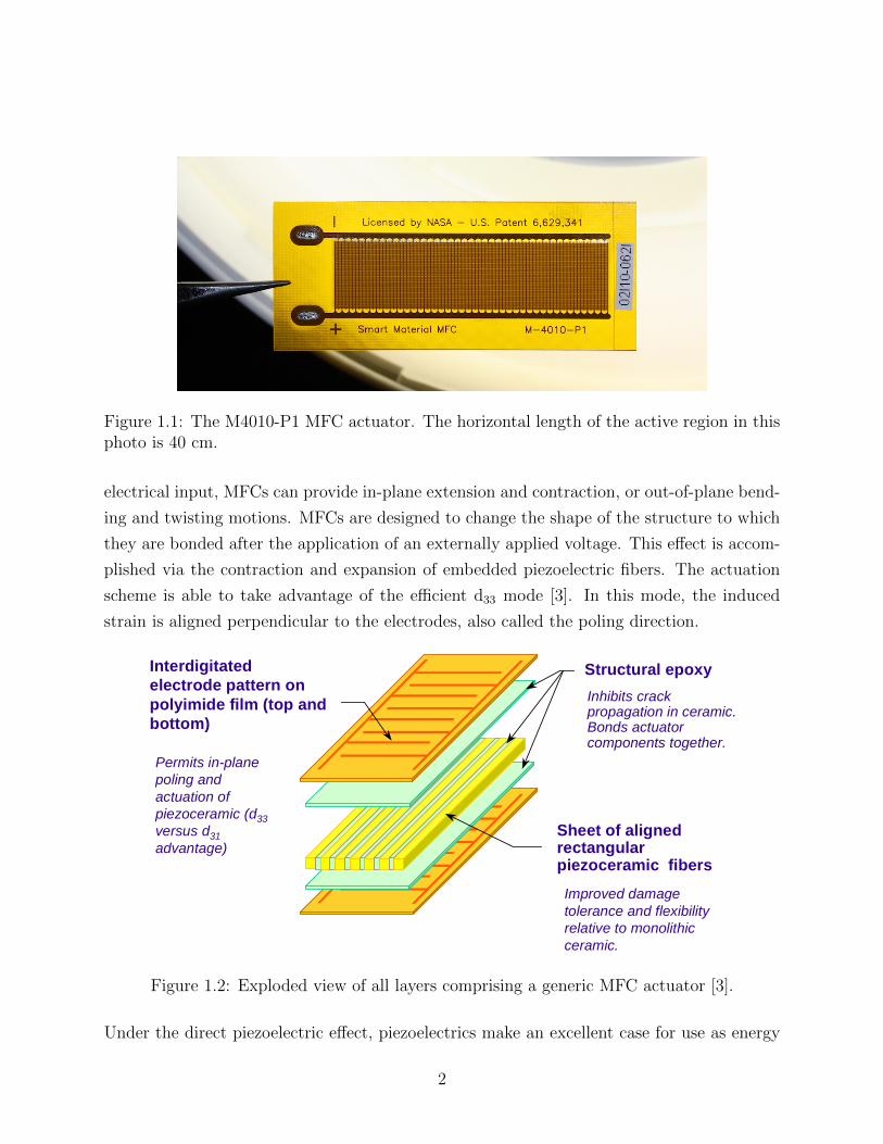
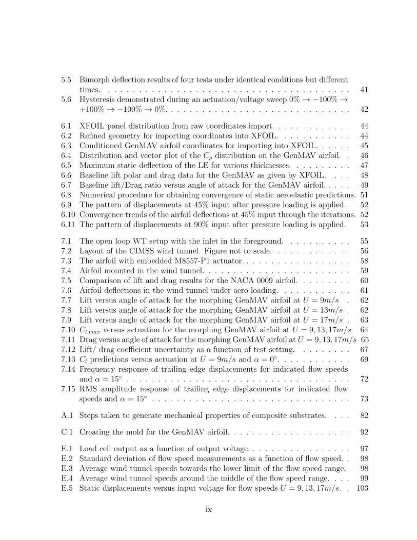
Figure 1.1: The M4010-P1 MFC actuator. The horizontal length of the active region in thisphoto is 40 cm.
electrical input, MFCs can provide in-plane extension and contraction, or out-of-plane bend-
ing and twisting motions. MFCs are designed to change the shape of the structure to which
they are bonded after the application of an externally applied voltage. This effect is accom-
plished via the contraction and expansion of embedded piezoelectric fibers. The actuation
scheme is able to take advantage of the efficient d33 mode [3]. In this mode, the induced
strain is aligned perpendicular to the electrodes, also called the poling direction.
Metallic interdigitated electrodes, etched or deposited, on polyimide film layers are placed next to the piezofibers forming thetop and bottom of the device. Protecting these fibers in a matrix polymer strengthens and protects the piezoceramic material.The resulting package is typically more flexible and conformable than similar actuators formed from monolithicpiezoceramic wafers. This allows the actuator package to be easily embedded within composite structures using conventionalcomposite manufacturing techniques. In addition, the use of interdigitated electrodes permits large, directional, in-planeactuation strains to be produced. The directional nature of this actuation is particularly useful for inducing shear, or twisting,deformations in structures.
The two principal disadvantages of piezoelectric fiber composite technology are the difficulty of processing and handlingexpensive piezoceramic fibers during actuator manufacture, and the high actuator voltage requirements [4]. Piezoelectricfiber composites have typically employed high cost, extruded, round piezoceramic fibers. Alternative methods ofconstruction using individual square cross-section fibers, diced from lower cost monolithic piezoceramic wafers, have alsobeen attempted, although sharp corners and edges of rolled square fibers have tended to damage or sever the interdigitatedelectrode fingers during the final actuator assembly process. Both round and square fiber approaches have requiredindividual handling of the piezoceramic fibers during the actuator assembly process, resulting in high manufacturing costs.An additional disadvantage with current piezoelectric fiber composite technology is high operating voltage requirements.Electrode voltages are primarily driven by the spacing, or pitch, of the interdigitated electrode fingers used to produce theactuation electrical field. A secondary factor tending to drive voltages higher is the attenuation of the driving electric field byunwanted accumulations of low dielectric matrix material between the electrodes and the piezoceramic elements. This resultsin reduced electrical efficiency of the actuator. Applying electrodes directly to the piezoceramic fibers, or otherwise placingthem in direct electrical contact with the piezoceramic, has proven to be difficult in practice.
The NASA Langley Research Center Macro-Fiber Composite actuator (LaRC-MFC ) is a recently developed deviceintended to mitigate many of the disadvantages associated with traditional piezocomposites. The LaRC-MFC retains themost advantageous features of active fiber composite actuators, namely, high strain energy density, directional actuation,conformability and durability, yet incorporates several new features, chief among these being the use of low-cost fabricationprocesses that are uniform and repeatable [11]. The Macro-Fiber Composite device will be described in the followingsections. The principal components and assembly of the actuator will be covered in detail, along with experimentalmeasurements of its performance. This paper concludes with a brief summary of several current applications projectsutilizing the MFC .
2. ACTUATOR MANUFACTURE
The primary components of the LaRC-MFC and their arrangement in the actuator package are illustrated in Figure 2. TheMFC actuator consists of three primary components: 1) a sheet of aligned piezoceramic fibers, 2) a pair of thin polymerfilms etched with a conductive electrode pattern and 3) an adhesive matrix material.
Sheet of alignedrectangularpiezoceramic fibersImproved damagetolerance and flexibilityrelative to monolithicceramic.
Structural epoxyInhibits crackpropagation in ceramic.Bonds actuatorcomponents together.
Interdigitatedelectrode pattern onpolyimide film (top andbottom)
Permits in-planepoling andactuation ofpiezoceramic (d33versus d31advantage)
Figure 2. Langley Macro-Fiber Composite actuator components.Figure 1.2: Exploded view of all layers comprising a generic MFC actuator [3].
Under the direct piezoelectric effect, piezoelectrics make an excellent case for use as energy
2

harvesters and sensors, since even slight deformations in the material tend to produce rel-
atively high voltages. This level of sensitivity from physical phenomena is highly desirable
for sensing applications. When utilizing the converse effect, piezoelectrics also demonstrate
the ability to deform in the presence of an electric field. Under actuation, the piezoelectric
effect causes a change in the geometry. Total stroke is limited since the effect is based on
a small-scale crystalline deformation [2], but strains on the order of 0.1% are not unusual.
Macro Fiber Composites do not escape the issues that inherently plague piezoelectrics, such
as poor repeatability and strains that are difficult to control.
MFCs come from a lineage of piezocomposites that have evolved over time to allow for
favorable operating characteristics, such as reduced brittleness and greater conformability.
Generally, MFCs are an advancement over active fiber composites (AFCs), which themselves
represent an improvement over first generation piezoelectric fiber composites (PFCs) [4].
This particular technology was selected for its fast response and high bandwidth nature,
which are critical in active structures.
In conventional aircraft, roll authority is achieved through movement of rigid aileron flaps
near the wing tips. Electromechanical (servo) or hydraulic motors articulate the flaps to
impart an effective change in camber [5], and alter the lift at this position of the wing.
In turn, an aircraft experiences a moment about its roll axis (a coupled yaw moment also
results if not trimmed). A thin wing found on an MAV provides no easy integration of
aileron-flap motors. On the other hand, MFCs are only around 0.3 mm thick; a beneficial
trait for use on thin wing aircraft. Mechanical linkages exterior to the wing can be costly
in terms of drag, weight, and power. The discontinuous joint created by the wing-flap
interface adds more drag. Embedded MFCs employ a bending motion to change wing camber,
increasing the lift coefficient and system performance over servomechanisms. The resulting
airfoil shape is continuous and more aerodynamically efficient. Maneuverability is improved
if the underlying structure is optimized for high frequency outputs.
3

1.2 Motivation
This thesis seeks to apply the foundation of available theories, software tools, and proper ex-
perimentation to a morphing airfoil so that an optimal active structure is designed. Actively
cambered airfoils have the possibility to offer performance enhancements, but traditional
design methods are not unanimously applicable. It is the purpose of this work to validate
and augment the processes pertaining to thin morphing airfoil analysis. To this end, a sys-
tems level approach is used that will consider all aspects of integrated MFC development.
Elements of aerospace, mechanical, and electrical design constitute the three primary facets
of development. This thesis will make use of a unique method to attain predictions on piezo-
electric based camber changes. Aero-structural effects will be studied with a newly defined
process and implemented with a common finite element package and aerodynamic predictive
software. New hardware to drive MFC actuators will be presented to fulfill power supply
requirements. Wind tunnel experimental results will enable comparisons with predictions to
ascertain model accuracy. To the authors knowledge, no previous work has been attempted
to encompass each of these aspects from the conceptual to testing stages using this method.
4

Chapter 2
Literature Review
Morphing wings concepts can be manifested variety of ways. All deviate from the notion
that the wing needs to be a rigid structure with fixed geometries. Wing area, sweep, di-
hedral, and camber are just some of the parameters with the potential to be changed by
infrequent or continuously variable mechanisms. Much focus has been placed on actuating
control surfaces, which offer the greatest capacity for performance improvements. This is a
form of maneuvering morphing, wherein the wing is changed to enhance flight control and
performance. In other morphing concepts, entire wing sections may fold unto themselves
or may reconfigure at a more infrequent basis. This expands the flight envelope to include
many distinctive missions achievable with a single platform. These are forms of configura-
tion morphing, which effect large changes in vehicle inertia, stability, and again performance.
Select examples are provided from the previous work of other researchers.
All morphing concepts open the door to a number of challenges involving structural and
aerodynamic design. Sophisticated analytical techniques have been used [6] [7] for modeling
piezoelectric stuctures, but they are difficult to use quickly for simple designs. This has
generated interest in modeling morphing effects with traditional finite element tools. A few
methods used in this work are presented here.
5

2.1 Active Wing Structures
2.1.1 Maneuverability Morphing
Use of piezoelectrics to effect wing shape control is not new. Vos, Brueker et al [8] demon-
strated morphing wing flight control via precompressed actuators on a unique semi-rigid
skinned airfoil. This thick airfoil combined a stiff NACA 0012 D-spar with a compliant
skin/bender mechanism on the aft portion of the 5.7 in chord. The dynamic motion of
the bender and skin was modeled using a the Rayleigh-Ritz method, Euler-Bernoulli beam
theory, and classical laminate theory (CLT). A net trailing edge (TE) deflection of 3.1 de-
livering a CLα of 1.72/rad was attained in wind tunnel tests. The system was subsequently
flown on a subscale UAV which exhibited a large gain in control authority.
Bilgen [9] developed a lightweight MAV with unimorph actuators. His initial investigation
used a Rayleigh-Ritz model to approximate structural deflections from MFCs. These results
were used to design the airfoil on a 0.76 m wingspan MAV, which demonstrated the validity of
thin cambered wings for use with MFCs. In flight testing, the durability of the flight control
devices came to light when numerous crash incidents were experienced. The structural
integrity of the MAV proved resilient and maintained sufficient roll control authority.
More recently, Bilgen [6] characterized a multitude of piezocomposite airfoils. These had
various implementations of MFC actuators, including unimorph and bimorph configurations
used for camber change and flow control. Compared to other piezoelectrics, he found MFCs
to be the most versatile, with other monolithic piezoelectric devices suffering from excessively
brittleness. Thin and thick airfoils were investigated for 2D lift and drag coefficients in low
Reynolds number flow. He demonstrated a maximum L/D of 17.8 for a flat plate airfoil
with two M8557-P1 bimorphs. This thin airfoil had a minimal 1 mil thick stainless steel
substrate and was able to maintain deflections under speeds around 45 m/s. The efficacy
of a compliant box-spar mechanism on a thicker airfoil was substantiated. Camber control
was not the sole focus of his work. Bilgen also studied the use of MFCs for flow control.
By exciting small MFCs near the leading edge (LE) of his airfoil at 125 Hz, a Cl,max gain of
27.5% was obtained. Additionally, various forms of high voltage drive circuitry are explored,
some of which are used in this thesis.
Using a Selig S1210 thick airfoil, Ohanian et al [10] introduced a novel design of trailing
edge camber control with MFCs. He cited the need for a solution to the separation inducing
6

flaps of traditional micro air vehicles at lower Reynolds numbers, pointing out the most
prominent benefits of MFCs, such as reduced drag, minimal added volume, and increased
relability due to less moving parts. The unique design includes numerous features meant
to prevent aerodynamic pressures from inhibiting the deflections from embedded bimorphs.
Aileron deflection tests demonstrated both the potential for large displacement amplitudes
and hysteresis effects of the actuator. Suggestions for open and closed loop control are made
in dealing with the hysteresis nonlinearities. Aerodynamic predictions based on experimental
bimorph deflections showed a possible ∆Cl of 2.25 due to MFC input, exceeding that of a
servo-actuated flapped airfoil.
In designing for camber morphing, Gandhi and Anusonti-Inthra [11] looked into the impli-
cations of control surface stiffness on actuation. They noted it is advantageous to have “low
in-plane axial stiffness but a high out-of-plane flexural stiffness,” the purpose of which is
to afford a reduction in the demands of camber change inducing technology (MFCs, SMAs,
etc.). They discovered a lower limit on these values that should be observed for reducing
undesirable deformation. The relevance of the paper deals with the tradeoff between rigid
structures that are capable of high aerodynamic loads and more flexible structures that allow
for high bandwidth technology to actuate them.
Kudva documents the DARPA Smart Wing [12] program as it has evolved since its inception
in 1995. This project was initiated to work on the application of smart materials to improve
the performance of military aircraft. Performance metrics were based on aerodynamic and
aeroelastic improvements. The article covers the two phases of the project that have since
been completed. Phases I and II both saw experimentation with Shape Memory Alloys
(SMAs) to actuate control surfaces. Early efforts brought out the bandwidth issues of SMAs.
During the second phase, a 30% scaled design with LE/TE active material appointments was
tested over a range of Mach 0.3 to 0.8, and resulted in significant performance improvements
(lift, roll rate). At such high dynamic pressures, the ability to retain control through use
of LE actuation at reduced aileron effectiveness was noted. The second phase of the Smart
Wing Project saw a UAV prototype that delivered a roll rate of 80/s. Another highlight
is the durability of the smart material designs. Kudva notably mentions that the “[Smart
Wing’s] control surfaces showed no degradation in performance during the three weeks of
wind tunnel testing.”
One of the largest projects undertaken in active wing development involved the Active Aeroe-
lastic Wing (AAW) program [13] by NASA, the Air Force Research Laboratory (AFRL), and
7

Boeing. The wings of an F/A-18 aircraft were re-engineered with a combination of thin alu-
minum and composite panels. The key parameter of effective wing torsional stiffness, which
enables active aeroelastic control, was experimentally determined. Overall stiffness decreased
17% from a standard F/A-18 wing. Leading and trailing edge control surfaces were driven by
hydraulics at lower dynamic pressures. Control at higher speeds was achieved with twist en-
abling “tabs”, to design around the common, albeit expected, aileron reversal issue at higher
Mach numbers. A new flight controller was developed by Boeing and NASA for the AAW
aircraft. An FEM delivered flutter predictions. Ground vibration testing matched modal
frequencies from the FEM with good accuracy. Roll data from in-flight testing at Mach
numbers between 0.8 and 1.2 demonstrated roll rates comparable to and sometime exceed-
ing that of traditional control surfaces. As one of the first forays into active wing structures
on a full scale air vehicle, the program has provided valuable insight in the multidisciplinary
requirements in active aeroelastic design.
2.1.2 Configuration Morphing
The utility of piezoelectric actuators is not limited to morphing for improved maneuverability.
Schultz [7] investigated their potential for snap-through shape changes, in which a laminate
substrate could be forced (snapped) into one of its multiple stable shapes. This would only
require a momentary input on behalf of an MFC. His focus is on unsymmetric laminates.
Due to their inherent property of being easily transformed into a new shape, they lend
themselves well to configuration morphing. To make predictions on the resulting shapes,
he applies classical laminate theory in combination with the Rayleigh-Ritz technique. He
was able to accurately predict snap-through behavior (resulting displacement fields) after
continually refining his model to include sensitive parameters such as final ply thicknesses
and orthotropic material properties. After fixing these issues, he emphasizes concerns with
piezoelectric and material nonlinearities.
Bowman et al [14] list the developments eminating from the Morphing Aircraft Structures
program from DARPA/AFRL/NextGen (NMAS). Thus far, the work has addressed poten-
tial benefits, important design features resulting from the program, wind tunnel tests, and
operational considerations. The flight envelope of a UAV usually falls under one or more
of the following modes: survive, attack, and loiter/reconnaissance. The authors attempt to
determine the optimal form of shape changes to most effectively operate in all three modes;
8
this is based on mathematical criterion examining the factors of loiter, dash times, and fuel
weight penalties. The NextGen morphing wing concept is then reviewed. A “batwing”-
resembling concept was ultimately chosen for the large range of attainable geometries. Skin
flexure was found to be the most critical design aspect. The tradeoff between adequate
flexibility and retaining flutter/ divergence margins was mentioned, but not detailed. What
emerged from this phase was a wing capable of an adjustable wing sweep between 15-45
and half-span of 7-10 ft. Uniquely, sweep and planform could be varied independently by
hydraulic actuators. Wind tunnel testing was completed at the NASA Transonic Dynamic
Tunnel, and met objectives such as operation under 2.5 G loading and transonic dynamic
pressures.
A 9.3 ft wingspan UAV designated Morphing Flight-vehicle Experimental 1(MFX-1) [15] was
developed by NextGen Aeronautics from the ground up to assess the practicality of in-flight
configuration morphing. An electric motor was employed to adjust wing sweep between 15-
35. Coupled movements from actuation simultaneously altered planform area by up to 40%.
This platform was successfully tested in speeds up to 120 knots. The impetus for this project
was derived from the NMAS program, which identified the need to characterize individual
morphing technologies before incorporating a suite of components onto a platform.
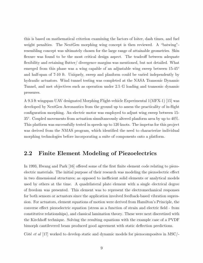
2.2 Finite Element Modeling of Piezoelectrics
In 1993, Hwang and Park [16] offered some of the first finite element code relating to piezo-
electric materials. The initial purpose of their research was modeling the piezoelectric effect
in two dimensional structures; as opposed to inefficient solid elements or analytical models
used by others at the time. A quadrilateral plate element with a single electrical degree
of freedom was presented. This element was to represent the electromechanical responses
for both sensors or actuators since the application involved feedback-based vibration supres-
sion. For actuators, element equations of motion were derived from Hamilton’s Principle, the
converse effect piezoelectric equation (stress as a function of strain and electric field - from
constitutive relationships), and classical lamination theory. These were next discretized with
the Kirchhoff technique. Solving the resulting equations with the example case of a PVDF
bimorph cantilevered beam produced good agreement with static deflection predictions.
Cote et al [17] worked to develop static and dynamic models for piezocomposites in MSC/-
9

NASTRAN. They cited the need for a common method to be used in designing piezoelectric
actuators bonded to composite structures, such as those used in the aerospace industry. They
foresee the use of a computational tool to describe the active regions incorporating piezo-
electric actuators and sensors. In this regard, a three dimensional model was used to gauge
the accuracy of using thermal strains in FEA to represent the converse piezoelectric effect.
Three dimensional elements were used in static and dynamic analyses. In their cantilevered
beam example, they found excellent correlation between the finite element model results and
numerical estimations. Experimental testing on dynamic behavior was less conclusive, and
Cote postulated on the effects of insulating layers used in fabrication.
Reaves discusses the need to be able to quickly implement piezoelectric actuators using FEA
[18]. In this regard, three approaches from previous research are outlined. The first in-
volves use of the thermal analogy to represent actuator induced strain. A second approach
from some researchers progressed to employing native elements incorporating the piezoelec-
tric effect within MSC/NASTRAN. Lastly, the prospect of coupled field elements offered
by ANSYS are of interest. Reaves indicates the need to validate these new methods with
experimental validation. He take advantage of these modelling techniques to fully charac-
terize piezoelectric systems with a focus on dynamic response. Overall, “global behavior”
such as steady state displacement and reasonant frequencies were well correlated between
the models and experiment. As with Cote [17], the bonding between actuator and substrate
was exposed as critical issue contributing to reduced model accuracy. Apart from a few
minor differences, the three approaches largely provided similar results.
10

Chapter 3
Mechanical Simulation with FEA
The following section will present the design and simulation methods for modeling MFC-
actuated airfoils. Each aspect of the final model from geometry and material generation is
discussed in detail. An electro-thermal analogy is derived to recreate the piezoelectric effect
in simulation. This culminates in an NX Nastran-produced [19] solution, which is compared
to experimental results in later chapters. NX Nastran is a commerically available software
tool built upon the NASTRAN code database developed by NASA [20]. Finite element
modeling is a practical method of delivering fast predictions for complex geometries, allowing
a broader scope of design areas to be investigated.
3.1 Airfoil Selection
The airfoil of interest is from the GenMAV, an aircraft design eminating from the AFRL but
evolved from a University of Florida design [21]. Its purpose is to test concepts related to
MAV design. The thin, cambered airfoil belonging to the GenMAV has a chord length of 5
in and was optimized for a low Reynolds number flight regime (8 · 104 − 2.4 · 105). The MAV
design specifies a 24 in span and incorporates various 3D features such as a dihedral angle
and an elliptical planform, the effects of which are not the immediate focus of this work. In
later analyses, the airfoil coordinates are imported into NX using a 7th-order spline.
11

0 0.2 0.4 0.6 0.8 1
0
0.05
0.1
x/c
y/c
Figure 3.1: The GenMAV airfoil shape.
3.2 Macro Fiber Composites Properties
A rectangular coordinate system is most suitable to represent MFC dimensions. Verification
of proper alignment is critical for non-isotropic materials. The X-axis and Y-axis are aligned
with the longitudinal (PZT fiber) and transverse (electrode) directions, respectively. Figure
3.2 correlates to the material property directions given in Table 3.1.
Figure 3.2: Reference directions for thermal analogy with respect to the alignment of elec-trodes.
The piezocomposite MFC material is not isotropic in nature. It is instead known to be
orthotropic, in which the material properties are defined by the three orthogonal directions.
Relevant orthotropic properties of MFCs have previously obtained by derivation and exper-
iment and are well established [4] [9]. These are listed alongside values provided by the
manufacturer in Table 3.1.
Macro Fiber Composites and their composite substrates are assumed to act in the linear
elastic regions of their respective materials. No loading from the actuators or aerodynamic
forces will be designed to take the material beyond the elastic region.
12

Table 3.1: Orthotropic properties of the MFC actuator by various sources.
Property MFC Datasheet [3] Williams [4] Bilgen [9]
Ex (GPa) 30.34 29.4 30.7Ey (GPa) 15.86 15.2 14.4Gxy (GPa) 5.52 6.06 4.10
νxy 0.31 0.312 0.267
Macro Fiber Composites are electrically equivalent to capacitors. Input voltages range from
-500 VDC to 1500 VDC . Although voltage requirements are relatively high, current draw is
quite low. Actual current draw is dependent on the form of drive circuitry (see Chapter 4).
Table 3.2 displays the electrical properties of the three different actuators used in this thesis.
Each product is offered by Smart-Material Corporation [3], Sarasota, FL.
Table 3.2: Electromechanical properties of the MFC actuator.
Model Length(mm) Width(mm) Cap.(nF) VRANGE(V)
M4010-P1 40 10 1.00 -500→1500M8514-P1 85 14 3.00 -500→1500M8528-P1 85 28 5.70 -500→1500M8557-P1 85 57 9.30 -500→1500
3.3 Composite Substrates
The core morphing wing design involves embedding MFCs into a wing to effect a change
in shape and gain favorable dynamic characteristics such as high roll control. As this calls
for an embedded actuator, special attention must be made to the material stiffness. The
actuator should function within design limits without experiencing excessive restriction in the
actuation direction. This compliance must also not be so great that the wing flutters under
normal operating conditions. Composites are the obvious substrate choice because they can
be tailored to the unique design requirements. Another benefit is the high strength-to-weight
ratios.
13

Due to the significant effect of substrate properties on actuation characteristics, an extended
derivation into the stiffness properties of composites laminate can be found in Appendix
A. A MATLAB program was written to quickly determine the sensitivity of material prop-
erties to various ply schedules. The ply schedule specifies the construction of the stack of
layers within a laminate, including (but not limited to) stacking sequence, ply orientation,
ply thickness. Figure 3.3 gives the reference directions and angles used with discussion of
laminate properties.
Figure 3.3: Illustration of laminate coordinate system with respect to fiber directions.
When designing the ply schedule of the substrate, a few considerations are made. In a sym-
metric laminate, the ply schedule is mirrored about the middle surface. For these laminates,
the bending-extension coupling matrix (Bij matrix of Appendix A Equation A.12) is zero.
This prevents bending from MFC actuation from inducing any coupling effects. Since the
wing structure is active by design, large deflections in an antisymmetric substrate could
produce undesirable geometry changes. An induced curvature is the only effect related to
camber control, so symmetric laminates are chosen for this suitable behavior.
Candidate materials for the composite substrates include E-Glass, S-Glass, and standard
modulus carbon fiber. E-Glass, or electrical-glass, is used in structural applications de-
manding low to moderate stiffness. Conveniently, the high resistivity and low dielectric [22]
of the fibers lends itself well to insulating embedded MFCs. S-Glass is both stiffer and
stronger than E-Glass. An intermediate/ standard modulus carbon fiber is significantly
stiffer and stronger than either of the glass products. Isotropic properties of theses materials
are outlined in Table 3.3.
Two dimensional elements are appropriate for modeling the behavior of laminates in FEA.
Since ply thicknesses are generally thin, a three dimensional model would require an inordi-
nate amount of elements to prevent poor aspect ratios. Only one material could constitute
14

Table 3.3: Relevant engineering properties of the constituent laminate materials.
Material: TensileModulus(GPa)
TensileStrength(GPa)
Poisson’sRatio
Density(kg/m3)
E-Glass (Fiber) [23] 72.4 3.45 0.22 2540S-Glass (Fiber) [23] 85.0 4.80 0.22 2480Std. Carbon (Fiber) [23] 230 3.53 0.20 1750Epoxy Resin [24] 2.81 0.054 0.236 –
each element. These restrictions would normally demand an elaborate model that accounted
for each separate ply in single-element thick sublaminates. Instead, the built-in NX laminate
modeler1 creates a physical property which can be applied to a 2D mesh. Within the mod-
eler, ply materials, scheduling, and thicknesses are specified. The entire analysis only covers
macroscopic effects such as displacement characteristics. Directly modeling the fiber-matrix
interface would be time consuming and is unnecessary. Instead, an homogeneous layer is
used to represent each ply.
Figures 3.4 - 3.5 feature the variation of orthotropic properties as a woven layer is rotated
between 0 ≤ θ ≤ 45 only. Beyond this angular range, the variation is symmetric for
45 ≤ θ ≤ 90 and then repeated for 90 ≤ θ ≤ 360. The variation of in-plane elastic
moduli Ebx and Eb
y show not much difference between E-Glass and S-Glass, but a large jump
in stiffness with carbon fiber. The largest disparity occurs for a ply orientation of 0.
The difference between shear moduli and Poisson’s ratio is largest at the 45 ply angle,
although very little shear deformation is expected for the thin laminates used as substrates.
These plots used ply stiffness properties from Table 3.4 using the process detailed in Appendix
B.
1The NX Laminates module optionally generates elastic moduli from constituent materials, but thisfunctionality is not used in this work.
15

Table 3.4: Orthotropic properties of various singles layer laminate plies.
Ply Description: Ex(GPa) Ey(GPa) Gxy(GPa) νxy
1 ply E-Glass 0/90 plain weave 23.71 23.71 3.10 0.091 ply S-Glass 0/90 plain weave 27.29 27.29 3.41 0.081 ply Std. CF 0/90 plain weave 63.72 63.72 3.31 0.041 ply Uni. Std. CF 0 116.41 10.66 3.31 0.22
0 5 10 15 20 25 30 35 40 450
10
20
30
40
50
60
70
Ply Orientation Angle (deg.)
Stif
fnes
s (G
Pa)
E−GlassS−GlassStd. Carbon Fiber
Figure 3.4: Variation of in-plane elastic moduli Ebx & Eb
y for a woven ply of various materials.
16

0 5 10 15 20 25 30 35 40 450
5
10
15
20
25
30
35
Ply Orientation Angle (deg.)
Stif
fnes
s (G
Pa)
E−GlassS−GlassStd. Carbon Fiber
0 5 10 15 20 25 30 35 40 450
0.1
0.2
0.3
0.4
0.5
0.6
0.7
0.8
0.9
Ply Orientation Angle (deg.)
E−GlassS−GlassStd. Carbon Fiber
Figure 3.5: Variation of shear modulus Gbxy (left) and in-plane Poissons νbxy (right) for a
woven ply of various materials.
17

3.4 Thermal Analogy
No method is available for directly modeling the piezoelectric effect in NX Nastran. The
piezoelectric-based MFCs are modeled instead using a thermal analogy. This derivation
uses a temperature input to represent the stress normally induced by placing a voltage
across the MFC leads. Although the physical properties of the piezocomposite devices are
in fact a function of temperature, this analysis will assume temperature effects are negligible
compared to the piezoelectric coupling effects. Starting with the constitutive equations for
piezoelectrics:
S = sET + dE (3.1)
D = dT + εE (3.2)
In the first equation, S is strain, s is the material compliance (the superscript E denotes a
short circuited condition), T is stress, d is the piezoelectric coupling coefficient, and E is
electric field. In the second equation, D is electric displacement, ε is the dielectric constant.
In this form, strain and electric displacement are functions of stress and electric field, though
this can easily be inverted to switch the independent and dependent variables. The simple
form of these equations is arrived under the assumption that the constants s, d, ε do not
to vary with stress or electric field. In reality, each coupling mode will saturate beyond
the linear region [25], but for this analysis those terms are still considered linear. Since an
important figure of merit for MFCs is the piezoelectric coefficient d, nonlinearity in this value
will be assessed in later analysis.
Equating strain induced by voltage to a simple strain induced by temperature:
εvoltage = εthermal (3.3)
[d] E = [α] ∆Θ (3.4)
Where α is the coefficient of thermal expansion and ∆Θ is the change in temperature. Now,
with V3 as the only direction of applied electric field:
18

d3i∆V3
∆el
= αi∆Θ i = 1, 2, 3 (3.5)
Where ∆el is the effective electrode spacing (constant). Equation 3.5 may be also be ex-
pressed:
d31∆el
d32∆el
d33∆el
∆V =
α1
α2
α3
∆Θ (3.6)
Ignoring the out-of-plane direction, renaming axes, and assuming 1:1 voltage to temperature
input:
[αx
αy
]=
d31∆el
d33∆el
=
−170pm/V0.459mm
−400pm/V0.459mm
=
−3.704 · 10−7 V −1
8.715 · 10−7 V −1
(3.7)
where α is the coefficient of thermal expansion in the x and y directions, d is the piezoelectric
strain coefficient term in the fiber and electrode directions, and ∆el is the effective electrode
spacing. The technique of this analogy is to simulate each voltage step 1:1 with each degree
of temperature difference. Since real temperature changes are not a focus, the coefficients of
thermal expansion for substrates and surrounding materials were not used.
The piezoelectric strain coefficient is not constant, however, and can vary with the magnitude
of the electric field or stress. For simplicity, a distinction can be made between high and low
electric fields. The manufacturer’s website [3] defines high field as those exhibiting greater
than 1 kV/mm. Noting the effective electrode spacing is 459 µm [6] for the MFCs:
Vhighfield ≥ Elimit ·∆el (3.8)
Vhighfield ≥ 1kV/mm · 459µm
Vhighfield ≥ 459V
19

The appropriate coefficient is used depending on the expected electric field. The change in
the coefficient for high and low electric fields is documented in Table 3.5.
3.5 Finite Element Modeling of Piezoelectric Strain
For the purpose of verifying the thermal analogy method, multiple tests cases were investi-
gated through finite element analysis. In its final form, the MFC actuation was implemented
as camber control on a morphing airfoil. The initial focus was on the ability of this airfoil
to create sufficient deflection from a neutral state.
Strain was modeled with 2D plate elements that represent the mid-surface of the real geom-
etry in the thickness direction. This assumption carries thin plate requirements, including
small out-of-plane thicknesses relative to in-plane dimensions. The actual theory used by
the NX Nastran solver is Mindlin-Reissner plate theory [20].
The various configurations included a plain MFC actuator, bimorph, and airfoil embedded
applications. Since the thickness of each configuration is small relative to span-wise and
chord-wise directions, all models were comprised of 2D CTRIA3 triangular and rectangular
CQUAD4 surface elements in NX Nastran to simulate thin plate behavior. Using plate
elements is remains valid when MFCs are modeled with substrates, since they will always be
thin materials as well. After meshing, an element shape check verifes there are no distorted
elements that exhibit excessive aspect ratios, warping, or other maladies.
Resulting nodal displacements were compared with predicted behavior and experimental
tests. Depending on the specific model, the TE deflection will often be used as a quantified
measure of actuator effectiveness due to substrate ply schedule, MFC placement, or other
implementation effect. Radius of curvature is also used as a means of comparison because
predicted curvatures are constant lengthwise along the model for simple bimorphs. This is
defined as the inverse of the curvature κ.
3.5.1 Application of Thermal Analogy
The first step in employing the thermal analogy is setting reference temperatures where
necessary to 0C. The choice of temperature units is arbitrary, given continuity with the
20

input temperature. Next, a thermal load numerically equivalent to the intended voltage is
applied to the nodes of the model that represent the active area of the MFC device. Gravity
was neglected for these test cases. The inactive area, primarily consisting of thin flexible
Kapton/epoxy layers, was also neglected.
Depending on the magnitude of the expected electric field between MFC electrodes, a co-
efficient of thermal expansion representing either a high- or low-field piezoelectric strain
coefficient is used. Table 3.5 gives the alpha values for the half-actuation range. Larger
coefficients are used with high field input (V > 459 V ). These values are entered into the
orthotropic properties for the MFC plies within the airfoil laminate model. Actuation level,
occasionally given with a percentage, is an arbitrary designation. Here, full positive actua-
tion (100%) symbolizes the input generating maximum downward movement of the TE or
maximum camber for any configuration.
Table 3.5: Thermal expansion coefficients representing the piezoelectric effect for variousvoltages.
Act.(%) VTopMFC(V) αTop
x (10−7) αTopy (10−7) VBot
MFC(V) αBotx (10−7) αBot
y (10−7)
0% 0.0 8.715 -3.704 0.0 -2.905 1.23512.5% 187.5 8.715 -3.704 -62.5 -2.905 1.23525.0% 375.0 8.715 -3.704 -125.0 -2.905 1.23537.5% 562.5 10.02 -4.575 -187.5 -2.905 1.23550.0% 750.0 10.02 -4.575 -250.0 -2.905 1.23562.5% 937.5 10.02 -4.575 -312.5 -2.905 1.23575.0% 1125.0 10.02 -4.575 -375.0 -2.905 1.23587.5% 1312.5 10.02 -4.575 -427.5 -3.341 1.525100.0% 1500.0 10.02 -4.575 -500.0 -3.341 1.525
As this macroscopic model is enabled only by an analogy to a true physical phenomenon,
limitations on the applicability should always be considered. Out-of-plane voltage variation
is assume constant and zero. Clearly, the domain of this analogous effect should never
exceed the input voltage limits of an MFC. Additionally, failure modes, operational lifetime
effects, nonlinearities in electromechanical properties, and effectiveness of dynamic behavior
predictions are not delivered here. The analogy was not formulated for sensing (direct effect)
applications.
21

3.5.2 Bare MFC
Generally, an MFC actuator exhibits expanding or contracting motion. The actuation mode
is controlled by the orientation of the electric field with respect to the PZT fibers. A bending
motion will result from electrodes running normal to the fibers, whereas twisting occurs if
the electrodes are at any angle offset from normal to the fibers.
A simple MFC is modeled without a substrate (Figure 3.6). Dimensions are taken from the
active area of an M8528-P1 MFC. Although this is not a useful real world implementation,
it is important nonetheless to verify the finite element model with proper constraints and
loading. After the geometry is meshed, the laminate property is applied to the mesh. A
temperature load of 100C is given to each of the 102 nodes, with one fixed constraint on
the center bottom node (shown at the left in Figure 3.6).
Figure 3.6: Bare MFC actuator with one fixed node and temperature-only loading (rotated90).
The predicted displacements in the X and Y directions are calculated with the temperature
induced strain equation.
∆lx = Lx(α∆T ) = 3.346 · (−3.704 · 10−7) · 100 = 2.916 · 10−4 in.
∆ly = Ly(α∆T ) = 1.102 · (8.715 · 10−7) · 100 = −4.082 · 10−5 in.
∆ly/2 = −2.041 · 10−5 in.
where ∆l is the change in overall length and L is the original length given in the two directions.
22
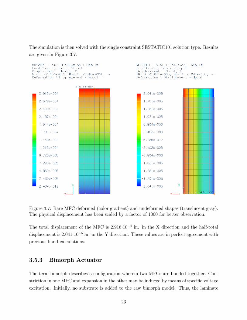
The simulation is then solved with the single constraint SESTATIC101 solution type. Results
are given in Figure 3.7.
Figure 3.7: Bare MFC deformed (color gradient) and undeformed shapes (translucent gray).The physical displacement has been scaled by a factor of 1000 for better observation.
The total displacement of the MFC is 2.916·10−4 in. in the X direction and the half-total
displacement is 2.041·10−5 in. in the Y direction. These values are in perfect agreement with
previous hand calculations.
3.5.3 Bimorph Actuator
The term bimorph describes a configuration wherein two MFCs are bonded together. Con-
striction in one MFC and expansion in the other may be induced by means of specific voltage
excitation. Initially, no substrate is added to the raw bimorph model. Thus, the laminate
23

construction is only comprised of two MFCs. This removes the possibility for any erroneous
results from substrate property estimations. The bond between the layers is assumed perfect.
Results are shown in Figure 3.8.
0 0.5 1 1.5 2 2.5 3
−1.5
−1
−0.5
0
0.5
Bimorph Location (in)
Bim
orphDisplacement(in)
0.0% ∆Zmax
=0.00", 1/κ = ∞
10.0% ∆Zmax
=0.06", 1/κ =90.9"
20.0% ∆Zmax
=0.12", 1/κ =45.7"
30.0% ∆Zmax
=0.20", 1/κ =27.6"
40.0% ∆Zmax
=0.26", 1/κ =20.9"
50.0% ∆Zmax
=0.32", 1/κ =16.9"
60.0% ∆Zmax
=0.39", 1/κ =14.2"
70.0% ∆Zmax
=0.45", 1/κ =12.3"
80.0% ∆Zmax
=0.53", 1/κ =10.5"
90.0% ∆Zmax
=0.59", 1/κ =9.5"
100.0% ∆Zmax
=0.65", 1/κ =8.6"
Figure 3.8: Predicted bimorph displacements from nonlinear solver. Tip displacements andcurvature radii are given in the legend.
Large out of plane deflections evident from a bimorph make a good statement for the use
of a nonlinear solver. Nonlinear structural analysis is required if a material is subjected
to strains beyond its elastic limit. Another complication includes geometric nonlinearity.
This situation presents itself when element displacements are large even though strain is still
linear. In a bimorph, each MFC has a fixed wall boundary condition and only the coupled
movement due to the bonding of the secondary MFC layer. For the static model-comparison
tests, there is no external loading or substrate present, which normally constrain bimorph
displacement. The largest predicted displacements are up to 20% of the original undeformed
length. The CQUAD4 elements that comprise the bimorph mesh are compatible with the
nonlinear static solution type NLSTATIC106 [20], which has the LGDISP parameter enabled
to account for geometric nonlinearities. When processing, the solver creates subcases that
incrementally load the part based on new geometry arrived at from previous (smaller) loads.
This loading is of purely thermal form.
Results from the nonlinear analysis show slightly reduced displacements. This reduction is
8.1% of the original curvature at the maximum actuation, and 3.6% at 50% actuation.
24

3.5.4 GenMAV
Two distinct layers are created as 2D surface of the GenMAV airfoil that has a 5.25 in span
and 5 in chord length. Refer to Appendix D for the coordinates of the airfoil shape. A
laminate sandwich structure with an embedded bimorph is then defined. The CAD model
of this is given in Figure 3.9. Table 3.6 documents the construction by breaking down the
components of each laminate.
Figure 3.9: Raised side view of the GenMAV airfoil, the orange region representing theembedded MFC actuator.
Table 3.6: Construction of laminate by color region of Figure 3.9. Glass-epoxy (or fiberglass)is denoted as “G/E”.
Region Ply Material Thickness αthermal
Orange
1 Top MFC 12mil αtopx 6= 0αtopy 6= 0
2 (3.16+1.45) oz/yd2 G/E 4.79mil αx = 0αy = 0
3 Bottom MFC 12mil αbotx = −αtop
x /3αboty = −αtop
y /3
Yellow1 (3.16+1.45) oz/yd2 G/E 4.79mil αx = 0
αy = 0
Setting a particular temperature for the top and bottom active area nodes cannot be done
separately, so the coefficients of thermal expansion are altered such that the induced strain is
25

not identical on the top and bottom physical surfaces. A bimorph creates a bending moment
by inducing a positive and negative strain on the top and bottom surfaces, respectively. This
issue is solved by negating and multiplying the coefficient of thermal expansion of the bottom
MFC by one-third. In this manner, any temperature simulated as a positive voltage on the
top MFC will be reflected by a negative voltage that is one-third of the top MFC voltage.
This properly reflects how asymmetric voltage is applied to the actuator.
Two primary factors govern the capability of the actuator. Material stiffness comes from the
elastic moduli, and the inertia component creates resistance to deformation. Beam curvature
is inversely proportional to the bending stiffness term EI. The largest curvature would be
experienced for the lowest material stiffness or inertia. Beam inertia is dominated by a cubed
thickness term.
A simple airfoil model is shown in Figure 3.9. The surface where the MFC would be bonded to
is the orange region, which follows the contour of the GenMAV profile. Two distinct surfaces
are meshed with element edges of 0.1 in. All edges of the inner surface are coincident with
the outer surface, and the edge nodes are shared. An example FEM is shown in Figure 3.10.
Mesh density has been reduced to more clearly indicate loading and boundary conditions.
A set of fixed nodes constrain the airfoil at a few edge nodes around the quarter chord to
simulate the presence of a supporting structure. For later wind tunnel testing, this represents
the load balance connection points. Nodes covering an area of around 0.01 in2 are fixed to
simulate these points, but this is exaggerated in Figure 3.10. The NLSTATIC106 solution
type is used to solve for the static deflection condition.
Figure 3.10: The finite element model showing placement of temperature loads and con-straints.
A mesh sensitivity test was completed for the GenMAV airfoil under 45% actuation. Meshes
26

were applied to the 2D surfaces with element edge lengths ranging from 0.5 in to 0.075 in.
Element sides with these lengths causes the number of elements to increase from 420 to 4830
after the automeshing. Sensitivity was quantified by observing the trend of TE deflection.
Little variation was recorded, even after increasing element count by an order of magnitude,
with the largest difference being 5.7%. This small difference can be attributed to the slight
changes in fixed boundary conditions due to the various mesh densities; that is, the area
(nominally 0.01 in2) assigned fixed nodes is not always the same. A final value of 0.1 in
(2600 elements) was chosen for all tests.
The full possible voltage (1500 V) is applied by setting the proper temperature of the sec-
ond laminate area’s nodes. After the NX Nastran solver has finished processing, the bulk
deformation of the airfoil is observed in Figure 3.11. The gray translucent outline is the
undeformed geometry.
Figure 3.11: Side view of the embedded bimorph actuator.
Actuator effectiveness at four chordwise stations is observed by measure of TE deflection
for three materials. Substrate ply schedule (thickness, orientation) is held constant. The
predicted static deflections from the FEM are plotted in Figure 3.12.
27

−0.1 −0.05 0 0.050.7
0.75
0.8
0.85
0.9
0.95
1
1.05
+x/c position of top MFC edge relative to QC
Norm
TE
Deflection
Before QC After QC
E-GlassS-GlassStd CF
Figure 3.12: Maximum static deflection of the airfoil for actuator placement at variouschordwise stations.
Placing the MFC closer to the quarter chord (QC) results in the greatest vertical stoke, and
substrate material is not a significant factor. If the assumption is made that macroscopic
mechanical effect is an equivalent bending moment, then it’s easier to understand that this
moment would be most effective at displacing the TE if it is applied at the fulcrum of the
airfoil. Conveniently, a stiffer LE required to transmit lifting loads becomes the preeminant
location for the front of the MFC actuator. After the chordwise position has been selected
as the quarter-chord, the most dominant parameter is then studied.
Ply orientation has the largest effect for low substrate thicknesses. Displacement becomes
mostly a function of thickness as that parameter increases. The predictions from Figure 3.13
are for E-Glass.
28

010
2030
40 2
4
6
8
0.4
0.5
0.6
0.7
0.8
0.9
1
Substrate Thickness (mil)Substrate Orientation (deg)
Nor
mal
ized
TE
Def
lect
ion
0.5
0.6
0.7
0.8
0.9
1
Figure 3.13: Maximum static deflection of the airfoil for various substrate orientation andthicknesses. Orientation angle is relative to the chord line.
29

Finally, Figure 3.14 shows maximum deflections for three materials and substrate thicknesses.
1 2 3 4 5 6 7 8 90.4
0.5
0.6
0.7
0.8
0.9
1
Substrate Thickness (mil)
Nor
mal
ized
TE
Def
lect
ion
E−GlassS−GlassStd CF
Figure 3.14: Maximum static deflection of the airfoil for various materials and thicknesses.Results are normalized to the greatest value within the plot.
Deflection does not seem to be a function of material. No optimal choice for thickness is
evident beyond the minimum. This will later be shown to be driven by stiffness constraints
defined by aerodynamic loading.
30

Chapter 4
MFC Driver Electronics
An important detail not to be neglected is the high voltage MFC drive circuitry. The key
goal of the drive circuitry is to actuate a bimorph MFC. The bimorph structure induces a
curvature by bending a beam with two actuators bonded on either side. Each individual
MFC exerts a maximum deflection at 1500 V of excitation, and minimum deflection at -500
V. To drive the two MFCs in every bimorph simultaneously, multiple independent voltage
supplies or a single supply with a unique voltage divider are required. The unique electrical
requirements of the MFCs have contributed to an “electronics gap” in the past and warrant
an extended look into circuitry that mitigates this issue.
4.1 Lightweight Circuit Prototype
As the airfoils presented here are designed for a small MAV, payload capabilities become a
critical design point. In the laboratory setting, high voltage amplification is achieved with a
13.2 kg 80 W bench top power amplifier. More compact commercial amplifiers are available
in power ranges around a few watts and weights around 50 g. This tradeoff is favorable, so
long as the drive circuitry is efficient and does not demand large currents exceeding tens of
milliamps. Due to limited market demands and recency of the MFC invention, there are no
devices available to drive MFC bimorphs with small package electronics.
31

4.1.1 Lightweight Circuit Schematic
At the heart of the design are three DC-DC converters from AM Power Systems, Dayton,
NV. These converters are single in, single out devices that operate in a manner such that
output voltage is directly proportional to input voltage.
Figure 4.1: Electrical schematic of the lightweight MFC driver PCB (courtesy Bilgen [26]).
In this arrangement, the third DC-DC converter supplies a fixed voltage to the ground
nodes of each MFC. This enables the other two converters to vary between 0 and 2000 V
and therefore place between -500 V and 1500 V across the capacitive load of each MFC.
Two analog output channels capable of 0-5 Vout and one fixed output are needed for control.
Slope change at zero volts can be handled by software providing the control. Figure 4.2
demonstrates the voltage output trends produced by the circuit.
A limitation of the DC-DC converters is the minimum output voltage. Although the specified
input range is 0 V to 5 V, the converters require at least 0.7 V to activate any output. The
linear output region of the converters begins around 0.9 V, which translates to a minimum
output of about 160 V. Note that the required changes do not affect the ultimate 1500 V
and -500 V output levels for the MFCs.
Situations where the MFC is charging are expected to occur very quickly, due to the nature
of the piezoelectric device. However, the system response when reducing the voltage across
MFC nodes is a concern. Since the MFCs act as capacitors, bleed resistors are connected to
drain the stored energy so that the physical deflection of the patch may decrease. Otherwise,
32

0
0.5
1
1.5
2
2.5
-100 -50 0 50 100
Voltage (kV)
Actuation (%)
DCDC 1
DCDC 2
Figure 4.2: The output voltages of the two variable output converters over the actuationrange.
there is limited control of the airfoil. Depending on the polarity of the voltage across their
terminals, the MFCs may want to discharge electricity to the left or right DC-DC converter
circuits. The diodes serve to prevent negative current from flowing through the converters
and damaging them.
Diode selection is critical for circuit operation. They prevent the energy stored in the MFC
patch from destroying the DC-DC converters when discharging. Proper selection requires
studying the expected conditions across the diode terminals. Should a sufficient reverse
voltage exist, the diodes could incur a reverse breakdown and they would allow harmful
current to pass into the DC-DC converters. A Vbr ≥ 5 kV will protect against load faults.
Bleed resistors around 5 MΩ were chosen after initial circuit tests. This was the lowest
resistance that allowed the DC-DC converters to reach the needed output voltage range.
Each control channel also required a separate power buffer to decouple signal voltage and
current draw from the control input.
The method for testing the control of an MFC actuated wing section starts with a LabVIEW
VI that formulates the appropriate signals based on high level commands. Two analog out
and one digital out channels of an NI USB-6009 DAQ then deliver these signals to the pro-
totype circuit. This hardware could be packaged into a complete flight-ready solution so
33

long as provisions exists for PWM-analog conversion for remote control compatibily with
commerical radio receivers. In a broader system level implementation with autonomy po-
tential, a microcontroller with a multichannel digital to analog converter chip would replace
the functionality of the NI DAQ.
4.1.2 Flight Weight PCB Design
If the unique voltage demands of the actuator cannot be satisfied by flight weight hardware,
then MFCs will not prove to be a viable form of camber control. Using the commerical
software program CadSoft EAGLE, the board in Figure 4.3 was developed as a proof of
concept that minimized all hardware dimensions and weight. The initial version of the
printed circuit board (PCB) weighed in at 32.5 g (for more details, refer to Appendix F).
Seen in Figure 4.3 is a two-sided revision that takes advantage of surface-mount devices
(SMDs). At half the size, this revision should bring the driver circuit weight to just 23.5 g.
A matching schematic is located in Appendix F.
Length, width, and thickness of the PCB is 3.75 in, 1.55 in, and 0.062 in, respectively. These
dimensions prove that this technology is in fact suitable for medium to large MAVs. Short,
direct traces and full solder masks are present to minimize potential high voltage shorting.
Additionally, a sizeable distance separates low voltage components from high voltage traces.
As shown, only the footprint of each DC-DC converter daughterboard is indicated. These
converters are not encapsulated to save weight. A weight breakdown of general equipment
used in the class of 2 lb electric MAVs is given in Table 4.1.
Table 4.1: Weights of standard MAV equipment and lightweight driver PCB (sorted bypercentage of overall weight).
Hardware Sample Product Weight (g) %
Battery EZ-Flite 351P 2600 mAh 200 60Brushless Motor Hacker A20-30M 150 W 45 13Radio Receiver Futaba FP-R127DF 7 Channel 40 12MFC Driver PCB – 32.5 10Motor ESC Castle Creations Phoenix-25 17 5
total: 334.5 100
34
+HV- +HV- +HV-
+LV- +LV- +LV-
E Gustafson 6/10 Rev.3
DC
DC
Con
v
DC
DC
Con
v
DC
DC
Con
v
D1
D2
D3
R7 R
8
R9
PW
R
R11
R12
R13
R14
R15
R16
R17
R18
R22
R23
R10
MFC
2-1
MFC
1-1
R19
R20
R21
T1 T2 T3
C1
R4
C3
R5
C5
R6IC1R1
R2
R3
C7
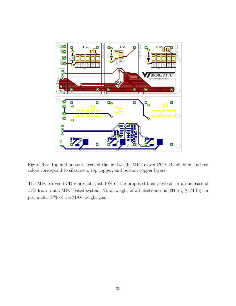
Figure 4.3: Top and bottom layers of the lightweight MFC driver PCB. Black, blue, and redcolors correspond to silkscreen, top copper, and bottom copper layers.
The MFC driver PCB represents just 10% of the proposed final payload, or an increase of
11% from a non-MFC based system. Total weight of all electronics is 334.5 g (0.74 lb), or
just under 37% of the MAV weight goal.
35
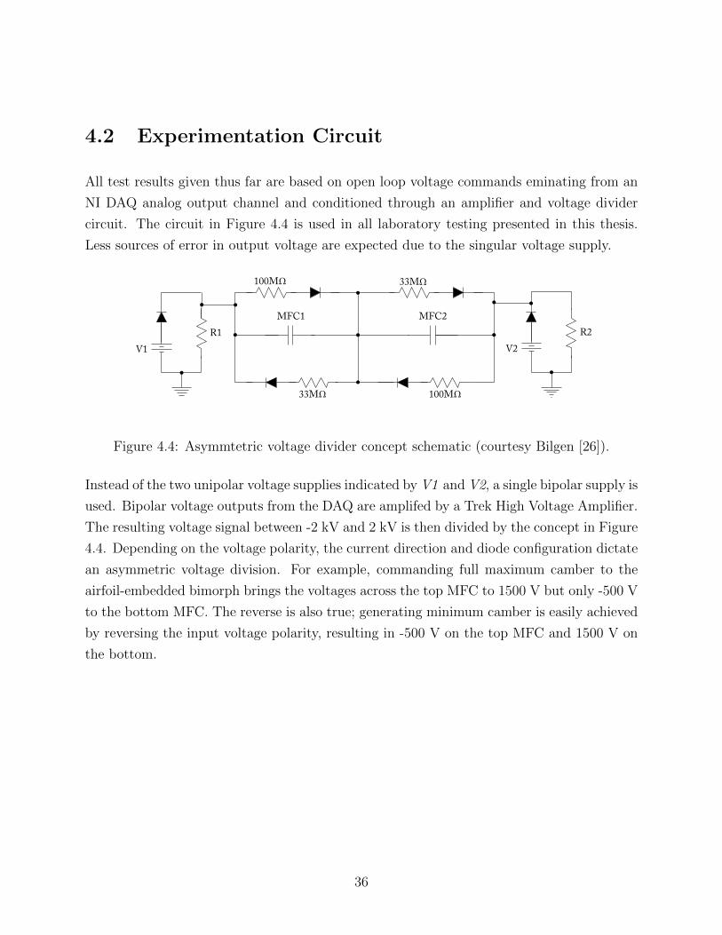
4.2 Experimentation Circuit
All test results given thus far are based on open loop voltage commands eminating from an
NI DAQ analog output channel and conditioned through an amplifier and voltage divider
circuit. The circuit in Figure 4.4 is used in all laboratory testing presented in this thesis.
Less sources of error in output voltage are expected due to the singular voltage supply.
MFC1 MFC2
100MΩ
V1
33MΩ
33MΩ
100MΩ
R1 V2
R2
Figure 4.4: Asymmtetric voltage divider concept schematic (courtesy Bilgen [26]).
Instead of the two unipolar voltage supplies indicated by V1 and V2, a single bipolar supply is
used. Bipolar voltage outputs from the DAQ are amplifed by a Trek High Voltage Amplifier.
The resulting voltage signal between -2 kV and 2 kV is then divided by the concept in Figure
4.4. Depending on the voltage polarity, the current direction and diode configuration dictate
an asymmetric voltage division. For example, commanding full maximum camber to the
airfoil-embedded bimorph brings the voltages across the top MFC to 1500 V but only -500 V
to the bottom MFC. The reverse is also true; generating minimum camber is easily achieved
by reversing the input voltage polarity, resulting in -500 V on the top MFC and 1500 V on
the bottom.
36

Chapter 5
Static Actuation Testing
Static testing was undertaken to verify the degree to which the model can accurately deter-
mine the displacements of the piezoelectric actuator. Experiments were completed with a
purpose-built rig capable of quantifying the entire deflection profile. These measurements
are plotted against the model.
5.1 Experimental Setup
A custom measurement system (Figure 5.1) with a laser displacement sensor mounted on a
computer numerical control (CNC) head is used to accurately measure the shape of the test
specimen under various actuations. The sensor is a Microtrak II-SA with a LTC300-200-SA
head delivering a resolution of ±20 µm, which interfaces with an NI USB-6216 16-bit DAQ
through an analog signal. The specimen is clamped at one end of the active area between two
nonconductive acrylic plates that are bolted together. This serves to create a fixed condition
which matches the model. The MFC is secured so that its thickness direction is orthogonal
to gravity. Since only static deflection is of interest, the voltage input is stepped at arbitrary
intervals over an arbitrary range (between ±100%). At each actuation level, the distance
between the specimen and the laser datum is measured along the middle of the specimen.
This occurs as the laser beam from the offset displacement sensor is translated along the
length of the specimen by the stepper motors of the CNC.
37

Figure 5.1: Experimental setup used to gauge bimorph shape under actuation for staticdeflection tests (not to scale).
Figure 5.2: Bimorph mount (left) and laser displacement sensor (right) used for static de-flection tests.
A Trek high voltage power supply combined with a custom circuit divider is used to drive
the bimorph. The schematic may be seen in Bilgen (2010 [26]). This circuit produces the
necessary bipolar asymmetric output to drive a bimorph up to its maximum input of 1500
V. As the Trek is capable of bipolar output (±2 kV), only this single supply is used. For
more detail, see Chapter 4.
The divider circuit utilizing high power resistors delivers bipolar asymmetric output. The
input and output voltages to this circuit for a test are recorded and shown in Figure 5.3.
38
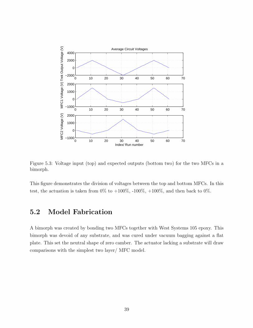
0 10 20 30 40 50 60 70−2000
0
2000
4000Average Circuit Voltages
Tre
k O
utpu
t Vol
tage
(V
)
0 10 20 30 40 50 60 70−1000
0
1000
2000
MF
C1
Vol
tage
(V
)
0 10 20 30 40 50 60 70−1000
0
1000
2000
Index/ Run number
MF
C2
Vol
tage
(V
)
Figure 5.3: Voltage input (top) and expected outputs (bottom two) for the two MFCs in abimorph.
This figure demonstrates the division of voltages between the top and bottom MFCs. In this
test, the actuation is taken from 0% to +100%, -100%, +100%, and then back to 0%.
5.2 Model Fabrication
A bimorph was created by bonding two MFCs together with West Systems 105 epoxy. This
bimorph was devoid of any substrate, and was cured under vacuum bagging against a flat
plate. This set the neutral shape of zero camber. The actuator lacking a substrate will draw
comparisons with the simplest two layer/ MFC model.
39

Figure 5.4: The zero camber bimorph used for model comparisons.
5.3 Model Comparison
The 100% actuation point was arbitrarily chosen for model comparisons. The zero camber
bimorph was brought to this level by manual control, and the measurement process was
initiated.
The first test’s results (Figure 5.5) were promising; actuator curvature was within 3.7% of
the model. Later tests showed increased output, even though no parameters are changed
beyond the order and test date. Of concern is the unpredicted increase in output that occurs
over testing intervals. The maximum strain evidenced by the large curvature induced by
a bimorph actuator causes significant shear at the ply interfaces. In this case, each MFC
represents one ply in a two ply laminate stack. Minimum curvature constraints (3.5 in when
curled longitudinally [3]) were not exceeded. Laminate delamination is a byproduct of exces-
sive loading, and manifests itself in small interlaminar voids. The increase in displacements
could potentially be attributed to delamination, which directly reduces bending stiffness [27].
The bonding epoxy is a product normally used as the matrix in composite materials. Other
researchers have used a high shear epoxies such as 3M DP460 [6]. Sizeable displacements
from these experiments combined with poor binding could have overstressed the bond and
allowed delamination. Shear stress is not transmitted through the voids, so the overall beam
experiences reduced stiffness and more pronounced deflections.
A more complicated cause could be interconnected electric fields of the top and bottom
MFCs. No electrical insulation is provided by the center thin epoxy or fiberglass layer.
40

0 0.5 1 1.5 2 2.5 3 3.5
−2
−1.5
−1
−0.5
0
0.5
Lengthwise Location (in)
Bim
orphDisplacement(in)
Exp 1; 1/κ= 8.14
Exp 2; 1/κ= 5.86
Exp 3; 1/κ= 4.24
Exp 4; 1/κ= 4.25
NX Nastran; 1/κ= 7.85
Figure 5.5: Bimorph deflection results of four tests under identical conditions but differenttimes.
Applying an electric field to one MFC may also induce the piezoelectric effect in the other,
given the inappreciable distance separating the MFCs. However, this does not explain initial
model agreement.
These tests also expose the hysteretic nature of piezoelectrics. Each test begins at a com-
pletely neutral camber/ curvature corresponding to the point at the origin of Figure 5.6.
The figure shows the maximum deflection results for the zero camber bimorph with the light
fiberglass substrate. As the voltage sweeps up and to the right to 100%, a different deflec-
tion trend is seen than when the actuator is brought from -100% to 100%. This is because
the trend is dependent upon the actuation history, and these are commonly referred to as
distinctive “sweep up” and “sweep down” motions.
41
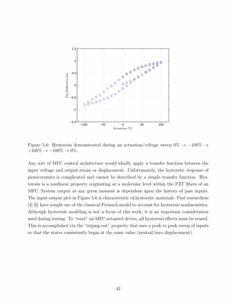
−100 −50 0 50 100−1.5
−1
−0.5
0
0.5
1
1.5
Actuation (%)
Tip
Deflection(in)
Figure 5.6: Hysteresis demonstrated during an actuation/voltage sweep 0% → −100% →+100%→ −100%→ 0%.
Any sort of MFC control architecture would ideally apply a transfer function between the
input voltage and output strain or displacement. Unfortunately, the hysteretic response of
piezoceramics is complicated and cannot be described by a simple transfer function. Hys-
teresis is a nonlinear property originating at a molecular level within the PZT fibers of an
MFC. System output at any given moment is dependent upon the history of past inputs.
The input-output plot in Figure 5.6 is characteristic of hysteretic materials. Past researchers
[4] [6] have sought use of the classical Preisach model to account for hysteresis nonlinearities.
Although hysteresis modeling is not a focus of this work, it is an important consideration
used during testing. To “reset” an MFC actuated device, all hysteresis effects must be erased.
This is accomplished via the “wiping-out” property that uses a peak to peak sweep of inputs
so that the states consistently begin at the same value (neutral/zero displacement).
42

Chapter 6
Aerodynamic Analysis
Aerodynamic characteristics are critical in quantifying the effectiveness of this form of mor-
phing control. In Chapter 3, actuation ability was predicted with no external forces. Now,
flow distributions will be used to predict airfoil geometry under aerodynamic loading. The
common software package XFOIL is used in this regard to accurately predict real world
capabilities.
6.1 XFOIL
The aerodynamic characteristics of the thin, cambered GenMAV airfoil were identified with
the XFOIL v6.9 program. XFOIL utilizes a combination of the traditional panel method
with compressibility corrections and the integral boundary layer method to solve for viscous
solutions. As a result, XFOIL can be used to accurately predict 2D airfoil characteristics in
low Reynolds number (Re) subsonic flow.
6.2 GenMAV
GenMAV airfoil coordinates shown as smooth splines are given in Figure 3.1. Unfortunately,
XFOIL has a known difficultly with obtaining the flow around thin airfoils with thicknesses
less than 1% of the chord (XFOIL documentation [28]). When the raw coordinates are
imported into the program, panels are auto-generated between the points in Figure 6.1.
43

The original set of coordinates results in 116 panel nodes and a maximum panel angle of
51.3o, which XFOIL then flags as excessive. While the number of panels along the top and
Figure 6.1: XFOIL panel distribution from raw coordinates import.
bottom surfaces may be sufficient, more attention is placed on the leading and trailing edges.
The geometry about these regions is very important. Thin airfoils are typically specified by
coordinates leading from the TE to the LE (or vice versa). Thickness is distributed by
offsetting the original coordinates by a finite value. Thin composite airfoils are usually
created by draping a fabric over a mold, so the thickness is plotted perpendicular to the
camber line. This results in a straight LE/TE with one panel. Nominally, there should be
multiple (>> 1) panels to describe this area. Convergence ability of the solution suffers
because of the non-smooth shape of the LE. This necessitates a modification, and a new
“false” round LE is generated only to enable this analysis. This will not affect the lift and
drag coefficients at any significant level, but will improve convergence tremendously [29].
Pelletier and Mueller [30] confirmed the lack of influence of LE and TE shapes experimentally.
Similarly, the TE is given a “false” wedge shape to aid in the application of the Kutta
condition.
−0.04 −0.02 0 0.02
−0.02
−0.01
0
0.01
0.02
0.03
0.04
x/c
y/c
0.85 0.9 0.95 1
−0.06
−0.04
−0.02
0
0.02
0.04
0.06
0.08
x/c
y/c
Figure 6.2: Refined leading edge (left) and trailing edge (right) geometries for importingcoordinates into XFOIL.
The number of panels generated by the airfoil coordinates alone is sufficient for a solution;
however, more panels are added to smooth results. The number of panels is generally around
44

150 panels (XFOILs imposes a limit of 177). A plot of the final airfoil coordinates is given
in Figure 6.3.
0 0.2 0.4 0.6 0.8 1−0.05
0
0.05
0.1
x/c
y/c
Figure 6.3: Conditioned GenMAV airfoil coordinates for importing into XFOIL.
6.3 Cp Distributions
Dimensionless Cp distribution is calculated and plotted with XFOIL for a 0 angle of at-
tack and three Reynolds numbers between 7.6(104) to 1.4(105). Test section turbulence is
accounted for with the transition criterion ncrit, which is kept at the default value for wind
tunnels with an average level of turbulence [28]. A visualization of the associated vectors
are simliarly shown in Figure 6.4.
The net upward pressure causes lift. Negative angles of attack progressively reduce this lift
and extend the downward suction near the LE on the bottom surface further along the chord.
The stagnation point just above the LE is responsible for the sudden jump in Cp. The flow
then accelerates and peaks in velocity around the maximum camber point on the top surface,
from where the majority of the lift is derived. A suction peak is also present just below the
LE; the cause of which is the very small leading edge radius. The suction is a counteracting
effect to the rapid change in flow direction around this edge. At sufficient magnitudes,
separation can occur due to an adverse pressure gradient. The net aero-structural effect is
muted, however, by the inherently thin LE.
Lift varies slightly with Reynolds number. In viscous mode, XFOIL makes predictions be-
tween the boundary layer and the flow field via integral boundary layer equations and the
eN method [28]. On this airfoil, it predicts separation and a drop in Cp to occur earlier for
increasing Re. This loss of lift occurs on the top surface due to a laminar separation bubble.
Laminar separation bubbles are a phenomena of low Reynolds number flow (104 < Re < 106).
They are formed when an adverse pressure gradient becomes significant enough to induce
rotational flow in the boundary layer [31]. This occurs when the laminar boundary layer
45

−0.2 0 0.2 0.4 0.6 0.8 1 1.2
−1
−0.8
−0.6
−0.4
−0.2
0
0.2
0.4
0.6
0.8
1
x/c
Cp
Top Surface - 76k
Bot Surface - 76k
Top Surface - 110k
Bot Surface - 110k
Top Surface - 140k
Bot Surface - 140k
Figure 6.4: Distribution (top) and vector plot (bottom) of the Cp distribution on the Gen-MAV airfoil. Note the ordinate is reversed.
separates and becomes turbulent, but a circulatory pocket of entrained flow forms in the
transitional region. Resulting separation explains the characteristic plateau and subsequent
drop in Cp developing between x/c=0.55 and x/c=0.65 in Figure 6.4. Likelihood of reat-
tachment decreases for Re > 5(104) [31], but the data show marginal reattachment of flow
near the TE.
In two dimensional analysis, spanwise effects are assumed negligible. This includes spanwise
flow interactions. Laminar separation bubbles and other boundary layer phenomena are
expected to hold constant over airfoil span. Realistically, some three dimensional effects
such as this are anticipated. Correction factors accounting for a constrained wind tunnel
test section are used to increase accuracy of predictions. Flow unsteadiness is assumed to
be of low magnitude and frequency; minor perturbations are averaged out by time weighted
data collection. The legitimacy of these assumptions will be assessed with a comparison of
analytical and experimental results in Chapter 7.
46

6.4 Refinement of Airfoil Design
It was discovered that aerodynamic loading had a pronounced effect upon the portion of
the airfoil between the LE and the quarter chord. In the model, the region covering the
LE was designed to incorporate two ply materials. The first corresponds to the ply that
covers the entire chord and acts as the actuator substrate. The second is a number of layers
of 0/90 woven carbon fiber used to transmit lifting loads to the main vehicle structure
(fuselage/frame). This second layer was initially designed to incorporate a single ply of 90
unidirectional carbon fiber. Analysis of aero-structural interactions showed this to be grossly
insufficient; large deflections at the LE were predicted. This led to the gradual addition of
individual plies to stiffen the LE of the model. In Figure 6.5, the maximum deflection is
recorded for various LE thicknesses, which relates to the ply count.
10 15 20 25 30 35 40 450
0.02
0.04
0.06
0.08
0.1
0.12
LE Thickness (mil)
LE
Deflection(in)
Figure 6.5: Maximum static downward deflection of the LE for various thicknesses. Resultsare normalized to the greatest value within the plot.
An obvious pattern of diminishing thickness effects are shown. From this figure, a minimum
thickness of about 0.04 in (40 mil) is chosen to be acceptable. This corresponds to four
woven plies of about 6.6 oz/yd2 carbon fiber.
47

6.5 Sectional Cd, Cl Predictions
A 5 in chord and flow speeds of 9, 13, and 17 m/s give a range 4.2(104) ≤ Rec ≤ 1.7(105).
The following lift polar and other plots are for a 0.8% thick GenMAV airfoil.
−5 0 5 10 15−0.5
0
0.5
1
1.5
Cl(2D)
α(deg)
−5 0 5 10 150
0.02
0.04
0.06
0.08
0.1
0.12
Cd(2D)
α(deg)
Re = 7.6(104)
Re = 1.1(105)
Re = 1.4(105)
Figure 6.6: Baseline lift polar and drag data for the GenMAV as given by XFOIL.
The standard GenMAV airfoil is predicted to stall around a 10 angle of attack, although
convergence at this point was not attained for the higher Re. This failure is most likely
due to XFOIL’s difficulty in determining larger regions of separated flow [28], therefore, it
is assumed that lift would taper or drop off anyway. The zero angle lift coefficient due to
airfoil camber is about 0.37, and Cl,max ≈1.4-1.45. Minimum drag occurs between 3-6. Lift
does not seem to be a function of Re for the range specified, but drag does show an upward
trend with Reynolds number near 5.
According to the results, L/Dmax increases from 46 to 59 over the Reynolds number range.
These peaks occur between 6-7. This closely matches the chosen incidence angle of the
standard GenMAV MAV [21].
48

−5 0 5 10 15−10
0
10
20
30
40
50
60
L/D(2D)
α(deg)
Re = 7.6(104)
Re = 1.1(105)
Re = 1.4(105)
Figure 6.7: Baseline lift/Drag ratio versus angle of attack for the GenMAV airfoil.
6.6 Static Aeroelastic Response
The methodology for predicting static aeroelastic behavior of a morphing airfoil is presented.
Pressure distributions over the GenMAV airfoil with a round LE and sharp TE are solved
with XFOIL. The airfoil is set at 1% thick due to the real expected thickness of a bimorph
actuator and optimized substrate. Non-dimensional pressure coefficients (Cp) are retrieved
from XFOIL solutions with the CPWR command under the viscous analysis menu OPER.
As purely a function of velocity ratio1 for incompressible flows [32], Cp results from the
XFOIL solution for a normalized airfoil may be extrapolated to different sized airfoils. Con-
sequently, Cp is scaled to the appropriate chord and then applied over the complete model
span. Pressures are calculated from Equation 6.1.
Cp ≡∆p
ρU2∞/2
(6.1)
A MATLAB mfile post-processes the raw output for proper importation into NX by sepa-
rating top and bottom pressure distributions into an intermediary data file. For 2D analysis,
spanwise pressure variation is assumed uniform and pressures on the infinitesimal leading
edge are ignored. Two boundary conditions with equivalent chordwise pressure distributions
are placed on the root and tip of the model airfoil. An interpolation routine in NX Nastran
delivers a spatial distribution of pressures along the airfoil span. Direction of the load on
1Ratio is between the local velocity UL along the airfoil surface and freestream velocity U∞
49
each element is determined by element orientation. Top and bottom pressures are applied
to the 2D mesh. The FEA model is solved in the same way as previous simulations. Nodal
displacements along the center span are saved into a new file. An assumption is made that
the displacements at this location are representative of the entire span. This is true in most
cases; only extremely thin substrates exterior to the bimorph location tend to invalidate the
assumption.
Another MATLAB mfile receives the nodal displacements and generates proper XFOIL co-
ordinates. The number of panels is correlated to the number of nodes along the chord on
the model. Additional datapoints augment the net panel count to around 149. Leading and
trailing edge treatments ease solution convergence. The entire process for converging upon
a final static displacement prediction is given in Figure 6.8.
The static aeroelastic deflections of the morphing GenMAV airfoil design in low speed flow
(9 m/s) is given in Figure 6.9.
50

Figure 6.8: Numerical procedure for obtaining convergence of static aeroelastic predictions.
51

0 0.5 1 1.5 2 2.5 3 3.5 4 4.5 5−1
−0.5
0
0.5
1
x (in)
z(in)
Initial GenMAV Coordinates
+45% Voltage Applied
+45% Voltage+Cp Loads Applied
Figure 6.9: The pattern of displacements at 45% input after pressure loading is applied.
Here, the change in relative displacement is shown after just five iterations. Convergence,
defined as less than 0.1% change in TE deflection, was achieved with only a few iterations.
An iterative process history showing solution convergence is given in Figure 6.10. As a
result of the stiffened region between the LE and QC and the chordwise placement of the
embedded actuator, the majority of the displacement occurs behind the QC location. This
effect is consistent for all simulated flow speeds and actuation input levels.
1 2 3 4 50.88
0.9
0.92
0.94
0.96
0.98
1
Iteration Number
TE
Deflection(norm
)
2 4 60
5
10
15
Iteration Number
%Difference
Figure 6.10: Convergence trends of the airfoil deflections at 45% input through the iterations.
The convergence trend of Figure 6.10 is common to all unlisted convergence plots. Looking at
the effect of higher aerodynamic loading, a flow of 17 m/s was simulated while the actuation
52

was set at 90% (Figure 6.11). As expected, the larger pressures from the higher speed cause
a greater loss of camber.
0 0.5 1 1.5 2 2.5 3 3.5 4 4.5 5−1
−0.5
0
0.5
1
x (in)
z(in)
Initial GenMAV Coordinates
+90% Voltage Applied
+90% Voltage+Cp Loads Applied
Figure 6.11: The pattern of displacements at 90% input after pressure loading is applied.
Static aeroelasticity assumes an equilibrium has been reached between aerodynamic and
elastic forces. Velocities and accelerations are assumed to have settled after solution conver-
gence. Temporal effects on system dynamics can be hidden by this assumption. This is why
experiments to validate the model are so critical.
53

Chapter 7
Wind Tunnel Testing
An overview of the wind tunnel facility with the instrumentation for data collection is dis-
cussed. This form of experimentation is the only method available for validating numerical
solutions obtained from aerodynamic analyses.
7.1 Wind Tunnel Facility and Instrumentation
Located in the CIMSS laboratory in Durham Hall on the Virginia Tech campus is a custom
open return type low speed subsonic wind tunnel built for past and present research on
MFC actuated airfoils. More in-depth construction details may be found in [6] and [9]. All
aerodynamic experiments listed in this thesis were completed at this facility.
Two fan stages produce airflow that is drawn through honeycomb flow straighteners at the
inlet, and then converged into the test section at a ratio of 5.9:1. The rectangular test
section is 35.6 x 13.6 cm in cross section and 91 cm in length. It can hold airfoil spans of 133
mm. Test section speeds are variable between 2.5 and 18.5 m/s. Flow speed steadiness is a
function of speed and activated fan stages. Tests demonstrating this variation are presented
in Appendix E. Overall length is 4.1 m. Two static ports and a FlowKinetics pitot-static
tube are connected to Setra and Dwyer differential pressure transducers, respectively. The
Setra unit is has a full range of 0-2.5 inH2O and 0.25% accuracy. The Dwyer transducer
has a 0-5 inH2O full scale range and 1% accuracy. An Omega thermocouple protrudes
into the test section to indirectly provide estimations of air density. An optoNCDT laser
54

Figure 7.1: The open loop WT setup with the inlet in the foreground.
displacement sensor with 0.01% full scale output accuracy is mounted along the test section
wall to gauge deflection distances from MFC actuation. Lift and drag forces are captured
by two Transducer Techniques 10 lb capacity load cells. All measurement devices are given
a minimum warm-up period of 30 minutes before data collection. Finally, a Canon S5-IS
camera is situated above the test section and takes photos of the airfoil cross-section.
The hardware for driving the MFCs includes a Trek High Voltage Amplifier and bipolar
asymmetric drive circuit detailed by Bilgen [26]. This amplifier also outputs the drive cir-
cuitry voltage and current draw as seen at the load output. An Oriental Motor Vextra stepper
motor and Velmex stepping motor controller can reposition the airfoil angle to within 0.1.
A small alignment jig provides the initial airfoil alignment of 0 relative to the wind tunnel
wall.
Both pressure transducers were calibrated against a Dwyer inclined differential manometer
under various dynamic pressures created by the wind tunnel between 0 and 1.78 inH2O. This
55

Figure 7.2: Layout of the CIMSS wind tunnel. Figure not to scale.
manometer had a sensitivity of 0.02 inH2O. The low pressure side of each pressure sensing
device was connected to the static pressure tap from the pitot-static tube, and the high
pressure side was connected to the stagnation pressure tap. The load cells were calibrated
by simulating a force at the middle of the test section, correlating to the center span of the
airfoil. This force was created by hanging precision weights from a cable/pulley assembly.
Velocity was deduced from a relationship between static pressure and dynamic pressure.
The static pressure was measured at the front of the test chamber. A factor related this to
dynamic pressure seen at the airfoil quarter chord location.
Data acquisition was handled by a National Instruments DAQ-Card 6062E and SCC-68
breakout box. All transducer channel voltages were polled by the onboard 12-bit A/D
converter at 100 hz over 5-10 seconds. The resulting data was time-averaged to filter noise.
This device interfaced with a standard PC running LabVIEW 2009 on top of Windows XP.
Hardware accessing each channel is outlined in Table 7.1 1.
Turbulence rejection is bolstered through use of honeycomb flow straighteners and screens.
Flow quality measurements were previous surveyed by Bilgen [6] [9] for an empty test section.
Turbulence intensity is a function of flow speed, but does not exceed 0.4% for the indicated
range. Freestream velocity varies by 4.5% and 1.5% in the horizontal and vertical directions,
respectively, but these deviations are not accounted for in later coefficient corrections.
1Servo PWM unused in the scope of this thesis
56

Table 7.1: All wind tunnel instrumentation hardware.
Ch Device Purpose
AO/0 Trek 623B High Voltage AmplifierAI/0 Setra 267 Pressure TransducerAI/1 Omega CCT-22 Air TemperatureAI/2 Trek 623B MFC Driver VoltageAI/3 optoNCDT ILD1800-200 Laser DisplacementAI/4 Dwyer 668-5 Pitot-Static Tube PressureAI/5 Trans. Tech. MLP10,TMO-2 Lift Load Cell/ Signal ConditionerAI/6 Trek 623B MFC Driver CurrentAI/7 Trans. Tech. MLP10,MO-1 Drag Load Cell/ Signal ConditionerD/3 Canon S5IS Camera Test Section PhotosC/0 Servo Motor PWM Flap Actuation
7.2 2D Lift & Drag Coefficients
A two-component load balance simutaneously measured lift and drag forces. The balance is
external to the test section. The part of the balance that holds the airfoil models is called
the “C-Arm”. Physical airfoil models with a constant 133 mm span and 127 mm chord are
vertically fixed to this C-Arm to cancel the effect of gravity. Aerodynamic loads are carried
by the fixture to the load balance and pivot table. These forces pivot the entire assembly
about a universal joint at the base, and in doing so apply an amplified force to the lift
and drag load cells which are aligned in their respective directions. In this manner, certain
configurations such as high angles and flow speeds in the upper range of the wind tunnel can
load the cells up to 80% of their capacity. The pivot table can change the angle of attack
by rotating the entire balance (C-Arm and counterweight). A 1-2 mm gap exists between
the model and test section wall on each side of the airfoil. This is mostly in the range of
acceptability as shown by Mueller and Burns [33]. Sectional lift and drag coefficients were
calculated in the following manner:
Cl =Fl
0.5ρV 2ACd =
Fd
0.5ρV 2A(7.1)
where Fl and Fd are the time averaged load cell outputs, ρ is the density of air, V is the
velocity calculated at the quarter chord, and A is the effective airfoil area. Wind tunnel
57

blockage and streamline curvature corrections were applied to lift and drag coefficients.
These are discussed in Appendix E.
7.3 Model Fabrication and Installation
Using the designs generated in Chapter 3 and construction procedure in Appendix C, the
morphing GenMAV airfoil was fabricated in-house. The ply schedule comprising the model
surface was laid up in a precision CNC-cut mold and vacuum bagged during the curing
process. Special care was taken with respect to MFC alignment during this step in order
to stay true to the previously determined layout. Excessive dimensions were trimmed to
produce an airfoil with a 127 mm chord and 133 mm span. A span of this length minimizes
the gap between the model and tunnel ceiling/ floor. Proper two dimensional flow requires
these gaps to be as small as possible.
Active Area1 MFC (top)
1 ply 4.6 oz/yd2 G/E [±45°]1 MFC (bottom)
1 ply 4.6 oz/yd2 G/E [±45°]
2 ply 6.6 oz/yd2 CF [0°/90°]1 ply 4.6 oz/yd2 G/E [±45°]2 ply 6.6 oz/yd2 CF [0°/90°]
1 ply 6.0 oz/yd2 CF [90°]1 ply 4.6 oz/yd2 G/E [±45°]
1 ply 4.6 oz/yd2 G/E [±45°]
Figure 7.3: The airfoil with embedded M8557-P1 actuator.
Post-cure, the model was removed from the mold. The edges were trimmmed to create a
133 mm span. Finally, 8-32 studs (not shown) were bonded to the thin airfoil at the quarter
chord with 3M DP460 epoxy. Extra care was taken to ensure the airfoil matched the design
as much as possible. The four requisite electrical connections to the MFC terminals were
insulated with Kapton tape to avoid exposure to conductive carbon fibers. Each of the four
wires inevitably adds bulk to the airfoil, so these were secured to the bottom surface and
covered with more tape to provide the smoothest surface possible.
The model was installed into the C-Arm fixture. Couplers were secured to the studs rigidly
58

Figure 7.4: Airfoil mounted in the wind tunnel.
fixed at the quarter chord. Final model weight is 31.5 g.
7.4 Reference Airfoil Investigation
For the purpose of validating the experimental wind tunnel setup, a reference NACA airfoil
was installed. The NACA 0009 airfoil with a 127 mm chord and 133 mm span was tested
under various angles of attack at a speed of 15 m/s and Re = 1.4(105). The airfoil was made
of rapid prototyping material. Baseline data for low Reynolds number flow was obtained
from Selig [34].
The lift predictions match up well. This load cell was calibrated only in the negative lift
direction, but this doesn’t seem to have any detrimental effect. The results reveal an un-
expected asymmetric drag for this airfoil. Minimum drag occurs at 2. A few explanations
59

−10 −5 0 5 10 15
−0.4
−0.2
0
0.2
0.4
0.6
0.8
1
1.2
Angle of Attack (deg.)
Lift
Coe
ffici
ent
V=
15.0
m/s
Experimental
Selig 100k
Selig 151k
dcl/dα = 2π
−10 −5 0 5 10 15 20−0.1
0
0.1
0.2
0.3
0.4
Angle of Attack (deg.)
Dra
g C
oeffi
cien
tV
=15
.0m
/s
Experimental
Selig 100k
Selig 151k
Figure 7.5: Comparison of lift and drag results for the NACA 0009 airfoil.
are provided for the admittedly high drag. During the load cell calibration process, a slight
cross-coupling between lift and drag load cell output was uncovered during drag calibra-
tions. Additionally, each measurement is very sensitive to external factors due the low
forces involved. The difficulty in ascertaining true drag should not be interpreted as though
experimental drag is useless; it still provides data for comparisons.
7.5 Experimental Procedure
A comprehensive LabVIEW Virtual Instrument (VI) was written to gather data from all
sensors and equipment shown in Table 7.1. A simple control file specifying flow speeds, angles
of attack, and voltage sweeps forms the only program input. Tunnel speed is manually set for
each desired Reynolds number. A velocity readout indicates the test section velocity, and the
variable autotransformer for fan control is adjusted until the readout settles on the desired
velocity. Airfoil angle of attack and MFC voltage sweeps are completely automated. At each
voltage (or actuation input), a 6 second delay waits for the airfoil to settle to a new static
position, and then 5 seconds of data are recorded at a frequency of 100 Hz. Simutaneously,
the camera is triggered to capture a photo of the deflection. Immediately before and after
each test, tare data are gathered from the lift and drag load cells for every angle of attack.
These data remove the effect of an uncanceled force due to airfoil weight. Lift and drag
coefficients ultimately quantify the aerodynamic characteristics of the mounted airfoil.
Although the wind tunnel is capable of flow speeds up to 18.5 m/s, undesirable vibrations
60

occur due to fan RPM (and possibly blade pass frequencies) at this level. This limit was
thus set at 17 m/s. Stall is expected to occur after 10 from XFOIL predictions, so the
angle of attack limit is given as 15. Voltage sweeps are stepped at 22.5% of the full range
(+337.5V/-112.5V). Total test time depends on the breadth and desired detail of the test,
but generally takes around 3 hours for each airfoil.
7.6 Results
All test results are gathered at once in the wind tunnel. Figure 7.6 gives a general idea
about the magnitude of actuator effectiveness of camber control while the test was being
completed. The figure shows minimum, neutral, and maximum deflections at α = 10 and
U = 9 m/s.
Figure 7.6: Airfoil deflections in the wind tunnel as seen aft of the test section. From left toright, -90%, 0%, and +90% actuation.
61

7.6.1 Sectional Cd and Cl Results
Lift and drag coefficients at flow speeds of 9, 13, and 17 m/s were obtained experimentally
and are shown in Figures 7.7-7.11. Lift coefficients taken for increasing angles of attack and
actuations are presented, along with XFOIL predictions at α = 0:
−10 −5 0 5 10 15 20−1
−0.5
0
0.5
1
1.5
2
LiftCoeffi
cient
V=9.0m/s
90%
67.5%
45%
22.5%
0%
-22.5%
-45%
-67.5%
-90%
Cl,α = 2π
Xfoil 9m/s
Angle of Attack (deg.)
Figure 7.7: Lift versus angle of attack for the morphing GenMAV airfoil at U = 9m/s
−10 0 10 20−1
−0.5
0
0.5
1
1.5
2
LiftCoeffi
cient
V=13.0m/s
90%
67.5%
45%
22.5%
0%
-22.5%
-45%
-67.5%
-90%
Cl,α = 2π
Xfoil 13m/s
Angle of Attack (deg.)
Figure 7.8: Lift versus angle of attack for the morphing GenMAV airfoil at U = 13m/s
All lift curves gradually plateau around 7.5. The slight uptick in lift at the highest angle
of attack is not considered useful due to limit cycle oscillations. At 9 m/s, predictions from
XFOIL correlate well with the experimental results when the airfoil is in a neutral state.
62

−10 0 10 20−1
−0.5
0
0.5
1
1.5
2
Angle of Attack (deg.)
LiftCoeffi
cient
V=17.0m/s
90%
67.5%
45%
22.5%
0%
-22.5%
-45%
-67.5%
-90%
Cl,α = 2π
Xfoil 17m/s
Figure 7.9: Lift versus angle of attack for the morphing GenMAV airfoil at U = 17m/s
Lift tapers off starting around 10, but it does not roll off as expected. Actuator effects
are evident in the offset lift slopes corresponding to various actuation levels. Reducing the
camber has a tendency to delay stall.
The bulk of the data exhibit linear lift responses with angle of attack. These extend to
around α ≈ 7.5 − 10, with the exception of large MFC inputs. As flow speeds increase,
the neutral input predictions fail to account for a lower lift curve slope. From photographic
data taken during testing, it is obvious that this is caused by aeroelastic deformations. The
benefit of being able to recover and then exceed the lost lift is afforded by the morphing
concept. Although the total authority of the aileron section would drop, it only takes around
a 22.5% input to restore the lift loss to the aeroelastic deformation. At 5, that level of input
gives the same amount of lift as the neutral shape at lower dynamic pressures.
63

−100 −50 0 50 100
0.7
0.8
0.9
1
1.1
1.2
1.3
1.4
1.5
Actuation %
Cl,max
9 m/s, Rec = 7.6 × 10⁴
13 m/s, Rec = 1.1 × 10⁵
17 m/s, Rec = 1.4 × 10⁵
Figure 7.10: Cl,max versus actuation for the morphing GenMAV airfoil at U = 9, 13, 17m/s
Maximum lift coefficient Cl,max peaks at 1.44 for 90% input and 9 m/s. The MFC actuators
afford increases of 10%, 11%, and 14% at the three respective flow speeds compared to a
neutral camber state. Dynamic pressure has a negative effect on the coefficient. As discussed
earlier, this is due to elastic deformations from aerodynamic pressure loading. On average,
this reduces Cl,max values 4.3% at 13 m/s compared to 9 m/s, and 8.1% at 17 m/s compared
to 9 m/s.
Drag coefficients taken for increasing angles of attack and actuations are presented in Figure
7.11.
64

−10 0 10 20−0.1
0
0.1
0.2
0.3
0.4DragCoeffi
cient
V=9.0m/s
−10 0 10 20−0.1
0
0.1
0.2
0.3
0.4
DragCoeffi
cient
V=13.0m/s
90%
67.5%
45%
22.5%
0%
-22.5%
-45%
-67.5%
-90%
Xfoil
−10 0 10 20−0.1
0
0.1
0.2
0.3
0.4
Angle of Attack (deg.)
DragCoeffi
cient
V=17.0m/s
Figure 7.11: Drag versus angle of attack for the morphing GenMAV airfoil at U =9, 13, 17m/s
As expected from the reference airfoil investigation, drag coefficients are higher than pre-
dicted. The angle for minimum drag shifts from 0-5 for instances of high camber to less than
0 for the lower camber. Higher flow speeds seem to reduce drag coefficient across all angles
and actuation levels. Drag normally rises with flow speed (Equation 7.1). The reduction is
another effect of the pressure loading.
65

7.6.2 Measurement Uncertainty
Uncertainties in sectional coefficients were determined in accordance with AIAA standards
[35] on wind tunnel testing. The coefficients arrive from three measurements: drag or lift
force, dynamic pressure, and area. Bias (systematic) and precision (random) errors from
each of those individual measurements contribute to overall coefficient uncertainty. Force
measurement uncertainties are combined from load cell and signal conditioner instrumental
errors. Pressure uncertainty is the result of a calibration process and elemental tranducer
errors. A small amount of uncertainty is added from measurement of the airfoil planform.
A 95% probability level is assumed for combination of elemental uncertainty sources and for
calculating component precision errors. Bias uncertainties are calculated by Equation 7.2:
Bc =
(J∑
i=1
[θiBi]2
)1/2
θi =∂r
∂Xi
(7.2)
where i is the index for bias uncertainties Bi and Xi is the measurement variable with
associated error sources. This equation omits correlated measurement effects because none
are made in the determination of lift/drag coefficients. Precision uncertainties are calculated
by Equation 7.3 since some, but not all, of the elemental errors are determined with averaged
readings:
Pc =
(J∑
i=1
[θiPi]2
)1/2
Pi =KSi√Ni
(7.3)
where i is the error source index and θi is defined as before. The precision limit Pi is a
function of K 1, measurement standard deviation Si, and the number of samples (readings) Ni.
Equations 7.2 and 7.3 account for the propagation of bias and precision limits. Cumulative
uncertainty in coefficient calculations is determined from Equation 7.4:
Uc =√B2
c + P 2c (7.4)
The constant bias errors are listed in Table 7.2.
1K is the coverage factor equalling 2 for a 95% confidence interval [35].
66

Table 7.2: Bias errors originating from transducers used in determining coefficients.
Bias Value Bi Measurement Xi Description of Error Source
BF = 0.068 N Lift or Drag Force Sensor-Transducer Stage, Signal ConditioningBQ = 3.32 Pa Dynamic Pressure Sensor-Transducer Stage, CalibrationBA = 46 mm2 Planform Area Instrument Resolution
Bias for lift and drag forces are equal because the same load cell type is used for both
measurements. Lift and drag coefficient uncertainties were calculated for the range of wind
tunnel conditions such as flow speed, angle of attack, and actuation input to the airfoil. Both
coefficient uncertainties were mostly a function of flow speed and voltage input. Precision
errors were significantly lower in magnitude than bias errors (just 3.6% in comparison, on
average), which were prominent for cases of negative actuation. Trailing edge deflection
above the original camber line counteracts the gain in lift due to airfoil camber, resulting in
very low forces to be measured by the load cells. This explains the peaks in uncertainty in
Figure 7.12.
0 100 200 300 400 500 600 7000.02
0.04
0.06
0.08
0.1
0.12
0.14
0.16
Setting/ Index Number
Coeffi
cientUncertainty
(dim
)
Cd uncertaintyCl uncertainty-100%
-100%
U = 13 m/s
U = 17 m/s
U = 9 m/s
Figure 7.12: Lift/ drag coefficient uncertainty as a function of test setting (setting # corre-lates to the progression of flow speeds, attack angles, and actuation levels). The three flowspeeds and first two peaks corresponding to minimum camber are indicated for clarity.
67

Table 7.3 charts the variation in maximum and average coefficient uncertainties for lift and
drag. Uncertainties peak at the lowest speed, but quickly drop off for higher speeds. The
overall average Ucd and Ucl are 0.061 and 0.054, respectively.
Table 7.3: Average and mean uncertainties for coefficients data.
Speed (m/s) Ucd mean Ucd max Ucl mean Ucl max
9.0 0.11 0.14 0.086 0.1513.0 0.047 0.057 0.047 0.06517.0 0.026 0.029 0.028 0.040
68

7.6.3 Model Comparison
A comparison made between wind tunnel data and Cl predictions that included coupled
aeroelastic effects is shown in Figure 7.13.
0 10 20 30 40 50 60 70 80 900.2
0.4
0.6
0.8
1
1.2
1.4
1.6
Actuation %
Cl
Predicted - No Cp
Predicted - With Cp
Measured - Corrected
Figure 7.13: Cl predictions versus actuation at U = 9m/s and α = 0.
The pressure loading had a greater effect on the lift characteristics than anticipated, es-
pecially at higher actuator input. As the actuation and camber increases, the actual lift
deviates from estimations more quickly. Aeroelastic predictions have an initial offset from
measured coefficients within uncertainty bounds, but with larger actuation, the predictions
account for a only portion of the reduced lift. The disparity could be attributed to separa-
tion regions that were larger than predictions. Experimental data were gathered from a test
that is 3D in nature; results are only post-processed into averaged 2D measurements after
the test is completed. This can obscure 3D effects, such as the complex trend of a laminar
separation bubble over the airfoil model span. Simliarly, gaps between the wind tunnel walls
at the airfoil root and tip were slightly larger than the recommended amount of 0.5% of
span. Due to manufacturing tolerances and the small airfoils of this class of air vehicles, the
gaps varied between 1-2% of the span. This could have introduced a larger than expected
vertical variation in flow speed within the tunnel. At the minimum, the nonlinearity should
be investigated in the future.
69

7.6.4 Limit Cycle Oscillations
Limit Cycle Oscillations (LCO) are a phenomenon characterized by sustained flow induced
vibrations. The mechanism by which this initiates is a coupled aero-structural problem.
If strong enough, aerodynamic pressures may induce an elastic deformation of a wing; the
deflection then changes the flow around the wing. In a situation where the wing deflects past
its neutral shape, the flow and elastic restoring forces change directions. The system may
devolve to constant vibration via positive feedback of the coupled motion. Traditional models
accounting for this effect describe the motions in a two degree of freedom model. Coupling
between the wing pitch and plunge displacements may lead to a net-positive amount of work
which may channel energy from the freestream into the the wing structure [36]. Oscillation
amplitudes may increase until structural failure. However, nonlinearities in the material
stiffnesses can limit excessive growth and instead allow for sustained oscillations (LCO).
Minimization of LCO is key in efforts to reduce fatigue and potential resulting damage
on wing structures. Nominally, aero-structures must be sufficiently stiff to prevent undue
vibrations.
Modeling LCOs with a composite airfoil design is exceedingly complex. A variety of ply
schedules create a spatial distribution of local orthotropic properties. Airfoil geometry and
strain is not constant and flucuates with MFC input. As such, wind tunnel testing is key in
identifying aeroelastic behavior of the airfoil design.
Airfoil oscillations were experienced under high aerodynamic loading. At high angles of at-
tack for the two higher flow speeds, the airfoil vibrates due insufficient chordwise stiffness.
Oscillations were measured with the optoNCDT laser displacement sensor already used to
gauge trailing edge deflections due to MFC input. In order to quantify the LCO effects,
amplitude and frequency measurements were included in post-processing. The NI DAQ is
set to queue analog input channels at 1000 hz1. Along with a 5 second collection period, a
spectral resolution of 0.2 hz is obtained. Input data is filtered with a 5th order Butterworth
filter with a cutoff frequency of 40 hz. Using MATLAB, one FFT is performed at each actu-
ation level, angle of attack, and flow speed. Peak frequencies were plotted versus actuation
level. Note that the actuation index refers to the level of voltage input as indicated in Table
7.4. The data indicate no clear resonant frequency for α < 15 and U = 9m/s. However,
the FFT plots specific to α = 15 at 13 and 17 m/s are given in Figure 7.14.
1A sampling frequency greater than 200 Hz is not really necessary, since oscillation frequencies are limitedby lower frequency airfoil dynamics.
70

Table 7.4: The voltages across the top and bottom MFCs embedded in the airfoil as afunction of the actuation index number.
Index # Act. % VtopMFC (V) Vbot
MFC (V)
0 0.0 0.0 0.01 22.5 337.5 -112.52 45.0 675.0 -225.03 67.5 1012.5 -337.54 90.0 1350.0 -450.05 67.5 1012.5 -337.56 45.0 675.0 -225.07 22.5 337.5 -112.58 0.0 0.0 0.09 -22.5 -112.5 337.510 -45.0 -225.0 675.011 -67.5 -337.5 1012.512 -90.0 -450.0 1350.013 -67.5 -337.5 1012.514 -45.0 -225.0 675.015 -22.5 -112.5 337.516 0.0 0.0 0.017 22.5 337.5 -112.518 45.0 675.0 -225.019 67.5 1012.5 -337.520 90.0 1350.0 -450.021 67.5 1012.5 -337.522 45.0 675.0 -225.023 22.5 337.5 -112.524 0.0 0.0 0.0
71

0 5 10 15 20 250
5
10
15
20
25
30Speed = 13m/s
Freq.(H
z)
Actuation Index 0-240 5 10 15 20 25
0
5
10
15
20
25
30
Freq.(H
z)
Actuation Index 0-24
Speed = 17m/s
90% 90%
-45%
-67.5%
-45%
Figure 7.14: Frequency response of trailing edge displacements for indicated flow speeds andα = 15
Figure 7.14 may be interpreted by understanding that a consistently horizontal line represents
a constant peak in frequency data across all actuation levels (−90% ≤ Act. ≤ 90%) from
the FFT. This is precisely what is observed for the speed and angle combinations in the
two subfigures. As the dynamic pressure rose, the random responses became more ordered.
Most of the data suggest a constant aeroelastic natural frequency centered around 25 hz.
The dips in peak frequencies occur around full negative actuation (minmum camber), where
no distinctive peak frequency is identifiable. This is most likely due to a cancelling effect of
reduced camber (lift detracting) and a high angle of attack (lift enhancing). The associated
mean zero data is simliarly plotted to obtain the RMS displacement amplitudes:
72

0 5 10 15 200
0.5
1
1.5
Peak RMS: 1.30 mm
Speed = 13m/s
Displacement
RMS(m
m)
Actuation Index 0-240 5 10 15 20
0
0.5
1
1.5
Peak RMS: 1.55 mm
Displacement
RMS(m
m)
Actuation Index 0-24
Speed = 17m/s
90% 90%
Figure 7.15: RMS amplitude response of trailing edge displacements for indicated flow speedsand α = 15
Average RMS displacement is 0.70 mm across all speeds and angles of attack. As before,
amplitudes only spike for α = 15 at 13 and 17 m/s. The peaks are consistent, occuring
between 67.5-90% actuation for each of the higher flow speeds. Peaks at these actuations
correspond to 204% and 183% gain in RMS amplitudes over the average. Aforementioned
average and peak amplitudes correspond to 0.6% and 1.1% of the chord dimension.
LCO behavior did not occur for the expected operating region of −5 ≤ α ≤ 10. The lift
curve trails off beyond 10 for the GenMAV airfoil. Evidence of this has been presented
analytically (Chapter 6) and experimentally. This analysis has shown that LCO only be-
comes in issue at extreme levels of aerodynamic loading exterior to a typical flight regime.
Additionally, the boundary conditions defined here do not necessarily reflect the final form.
The two fixed points at either end of the quarter cord on the airfoil only serve to allow for
the 2D measurements. The LCO observed here are not inexorably linked to the morphing
GenMAV airfoil.
73

Chapter 8
Conclusion
8.1 Summary
Seeking to utilize a promising new actuator that affords an efficient means of shape control,
an investigation was undertaken that applied morphing capability to an airfoil. A two
dimensional analysis of the GenMAV airfoil design judged the morphing effects over the
baseline shape. The orthotropic elastic properties of a composite substrate were optimized
for maximum shape control authority, leading to a highly tailored ply schedule. A thermal
analogy was used to represent piezoelectric strain. The applicability of using FEA to predict
large structural displacements was assessed. Deflection tests initially demonstrated good
agreement with the model, matching beam curvature predictions to within 3.7%. However,
significant out of plane bending was thought to have caused minor delaminations in the
zero-substrate test bimorph.
Minute treatments to the airfoil coordinates’ leading and trailing edges were required to
enable viscous analysis with the XFOIL program. The Reynolds number was shown to have
little influence on sectional lift and drag characteristics of the GenMAV airfoil. A Cl,max of
1.45 at 10 and Cd,0 of 0.02 at 5 were estimated. Subjecting the airfoil to various dynamic
pressures was simulated with both XFOIL and NX NASTRAN software. The coupling
between pressure loading and elastic deformations was iteratively calculated. The dominant
parameter affecting camber changes was found to be airfoil thickness. Substrate material
effects were inappreciable, and the selection was driven by the insulating electrical properties
of E-Glass. Morphing implications on static aeroelasticity were predicted.
74

The extensive set of equipment used to obtain lift and drag coefficients in wind tunnel test-
ing was discussed. A brief explanation on fabrication procedures of the morphing GenMAV
airfoil was provided. To validate the wind tunnel apparatus, the lift and drag characteristics
of a reference NACA 0009 airfoil were assessed. Lift data showed excellent correlation to
data provided by previous researchers, although drag was more pronounced. Sectional lift
and drag for the GenMAV airfoil matched up well with XFOIL estimations at lower dynamic
pressures. At 9 m/s and 0, a Cl of 0.4 and Cl,max of 1.0 were found. Similarly important,
a ∆Cl range of +0.6/-1.1 at this angle indicates the large working lift domain due to the
piezoelectric effect. With the ability to change the camber, the absolute Cl,max is attainable
at lower attack angles. Aeroelastic results showed a nonlinear trend of Cl that was under-
predicted under higher actuations. Experiments also exposed some LCO effects for limited
situations, but the two fixed point wind tunnel model doesn’t completely reflect real world
boundary conditions.
Lastly, a lightweight circuit prototype was developed to prove that the electrical demands
of the actuator did not require any hardware unusually large for an MAV platform. A 32.5
g proof of concept circuit board was fabricated and verified. A second revision condensed
the hardware to an estimated weight of 23 g. The final weight is within acceptable MAV
payload limits.
The cumulative contribution of this work was the application of morphing wing technology
to a standard MAV. Airfoil dimensions accomodated the application of MFCs very well;
most practically due to the thin nature of wings in this vehicle class. The GenMAV in
particular provides a good base of comparisons, since data from aerodynamic modeling and
wind tunnel testing are already freely available [21].
75

8.2 Recommendations of Future Work
In this thesis, practical airfoil designs were created for a single bimorph comprised of one
MFC type. That actuator is the M8557-P1 product from Smart-Material Corporation. This
company offers more MFCs that have scaled down in-plane dimensions, but are based on
the same piezoelectric principle. Such actuators may be advantageous to vehicle design with
reduced weight. Further analysis of morphing airfoils with various distributions of smaller
MFCs will determine if these versions are just as effective. These will be characterized by
continued wind tunnel testing at the same facility.
A good portion of research remains on identifing the bandwidth characteristics of embedded
bimorphs on the thin airfoil. The effectiveness of the thermal analog to predict dynamic
response was not quanitifed. The question of how to simulate the response under steady and
unsteady aerodynamic loading is also left open (dynamic aeroelasticity).
This thesis was limited to two dimensional analyses and experiments. Only chordwise ef-
fects of bimorph placement were studied. There are a myriad of ways to implement wing
morphing with MFC bimorphs; this is the benefit afforded to an embeddable actuator. The
purpose of the airfoil research is a lead-up to a complete wing and vehicle design. Air vehicle
design evaluations will require a larger wind tunnel so that three dimensional effects may be
measured.
Continued efforts in aeroelastic tailoring can eliminate the limit cycle oscillations existing at
higher aerodynamic loading. It may be prove favorable to trade deformability for a larger
safety factor against LCO.
76

Bibliography
[1] Wilkie, W. K., Bryant, R. G., High, J. W., Fox, R. L., Ileilbaum, R. F., Jr., A. J.,
Little., B. D., and Mirick, P. H., “Low-Cost Piezocomposite Actuator for Structural
Control Applications,” NASA Langley Research Center, Newport Beach, CA, March
2000.
[2] Kurdila, A., “Active Materials and Smart Structures,” ME5804 Lecture, Virginia Poly-
technic Institute and State University.
[3] Smart Material Corporation, May 2011,
http://www.smart-material.com/MFC-product-main.html.
[4] Williams, R. B., Nonlinear Mechanical and Actuation Characterization of Piezoceramic
Fiber Composites , Ph.D. thesis, Virginia Polytechnic Institute and State University,
2004.
[5] Houghton, E. and Carpenter, P., Aerodynamics for Engineering Students , Butterworth-
Heinemann, 5th ed., 2003, p. 182.
[6] Bilgen, O., Aerodynamic and Electromechanical Design, Modeling, and Implementation
of Piezocomposite Airfoils , Ph.D. thesis, Virginia Polytechnic Institute and State Uni-
versity, 2010.
[7] Schultz, M. R., Use of Piezoelectric Actuators To Effect Snap-Through Behavior Of
Unsymmetric Composite Laminates , Ph.D. thesis, Virginia Polytechnic Institute and
State University, 2003.
[8] Vos, R., Breuker, R. D., Barrett, R., and Tiso, P., “Morphing Wing Flight Control Via
Postbuckled Precompressed Piezoelectric Actuators,” Journal of Aircraft , 2007.
77

[9] Bilgen, O., Macro Fiber Composite Actuated Unmanned Air Vehicles: Design, Develop-
ment, and Testing , Master’s thesis, Virginia Polytechnic Institute and State University,
2007.
[10] III, O. J. O., Karni, E. D., Olien, C. C., Gustafson, E. A., Kochersberger, K. B.,
Gelhausen, P. A., and Brown, B. L., “Piezoelectric composite morphing control surfaces
for unmanned aerial vehicles,” Vol. 7981, SPIE, 2011.
[11] Gandhi, F. and Anusonti-Inthra, P., “Skin design studies for variable camber morphing
airfoils,” Smart Materials and Structures , Vol. 17, 2008.
[12] Kudva, J., “Overview of the DARPA Smart Wing Project,” Journal of Intelligent Ma-
terial Systems and Structures , Vol. 15, 2004, pp. 261–267.
[13] Pendleton, E., Flick, P., Paul, D., Voracek, D., Reichenbach, E., and Griffin, K.,
“The X-53, A Summary of the Active Aeroelastic Wing Flight Research Proram,”
AIAA/ASME/ASCE/AHS/ASC Structures, Structural Dynamics, and Materials Con-
ference, April 2007.
[14] Bowman, J., Sanders, B., Cannon, B., Kudva, J., Joshi, S., and Weisshaar, T., “Devel-
opment of Next-Generation Morphing Aircraft Structures,” AIAA/ASME/ASCE/AH-
S/ASC Structures, Structural Dynamics, and Materials Conference, April 2007.
[15] Flanagan, J. S., Strutzenberg, R. C., Myers, R. B., and Rodrian, J. E., “Develop-
ment and Flight Testing of a Morphing Aircraft, the NextGen MFX-1,” AIAA/AS-
ME/ASCE/AHS/ASC Structures, Structural Dynamics, and Materials Conference,
April 2007.
[16] Hwang, W.-S. and Park, H., “Finite Element Modeling of Piezoelectric Sensors and
Actuators,” Journal of Intelligent Material Systems and Structures , Vol. 31, No. 5,
May 1993, pp. 930–937.
[17] Cote, F., Masson, P., Mrad, N., and Cotoni, V., “Dynamic and static modelling of
piezoelectric composite structures using a thermal analogy with MSC/NASTRAN,”
Composite Structures , Vol. 65, No. 3-4, 2004, pp. 471–484.
[18] Reaves, M. C. and Horta, L. G., “Test Cases For Modeling And Validation Of Structures
With Piezoelectric Actuators,” 42nd AIAA/ASME/ASCE/AHS/ASC Structure and
Structural Dynamics Conference, April 2001.
78

[19] NX7, S. P., “Siemens PLM, Plano, TX,” 2010.
[20] Siemens PLM Software Inc., NX Nastran 7 Element Library Reference, 2009.
[21] Stewart, K., Wagener, J., Abate, G., and Salichon, M., “Design of the Air Force Research
Laboratory Micro Aerial Vehicle Research Configuration,” Proceedings of AIAA, 2007.
[22] Baker, A., Dutton, S., and Kelly, D., Composite Materials for Aircraft Structures , Amer-
ican Institute of Aeronautics and Astronautics, 2004, pp. 57,119.
[23] Hexcel Corporation, Technical Fabrics Handbook , 2010.
[24] West System, Typical Physical Properties .
[25] Leo, D. J., Engineering Analysis of Smart Material Systems , Wiley, 2007.
[26] Bilgen, O., Kochersbeger, K. B., Inman, D. J., and III, O. J. O., “Lightweight High Volt-
age Electronic Circuits for Piezoelectric Composite Actuators,” Journal of Intelligent
Material Systems and Structures , Vol. 0, 2010.
[27] Kollar, L. P. and Springer, G. S., Mechanics of Composite Structures , Cambridge Uni-
versity Press, 2003.
[28] Drela, M., “XFOIL 6.9 User Primer (User Documentaion),” .
[29] Reid, M. R., Thin/Cambered/Reflexed Airfoil Development for Micro-Air Vehicles at
Reynolds Numbers of 60,000 to 150,000 , Master’s thesis, Rochester Institute of Tech-
nology, 2006.
[30] Pelletier, A. and Mueller, T. J., “Low Reynolds Number Aerodynamics of Low-Aspect-
Ratio, Thin/Flat/Cambered-Plate Wings,” Journal of Aircraft , Vol. 37, 2000, pp. 825–
832.
[31] Gad-El-Hak, M., Flow Control: Active, Passive, and Reactive Flow Management , Cam-
bridge University Press, 1st ed., 2000, pp. 192–193.
[32] Shevell, R. S., Fundamentals of Flight , Prentice Hall, 2nd ed., 1989.
[33] Mueller, T. and Burns, T., “Experimental Studies of the Eppler 61 Airfoil at Low
Reynolds Numbers,” AIAA, 1982.
79
[34] Selig, M. S., Donovan, J. F., and Fraser, D. B., Airfoils at Low Speeds , H. A. Stokely,
1989.
[35] American Institute of Astronautics and Aeronautics, Assessment of Experimental Un-
certainty with Application to Wind Tunnel Testing , 1999.
[36] Mazet, R., Manual On Aeroelasticity , Vol. 1, North Atlantic Treaty Organization Ad-
visory Group for Aerospace Research and Development, 1968, pp. 1–51.
[37] Barbero, E. J., Finite Element Analysis of Composite Materials , CRC Press, 2007.
[38] Barbero, E. J., Introduction to Composite Materials Design, CRC Press, 1998.
[39] Barlow, J. B., Rae, W. H., and Pope, A., Low-Speed Wind Tunnel Testing , John Wiley
& Sons, 3rd ed., 1999.
80

Appendix A
Generating Laminate Stiffness
Properties
Substrate effects are the critical driven requirement to actuator design. The substrate itself
may be thought of as a passive component of the MFC actuator in unimorph or bimorph con-
figurations. Before a study of all possible effects may be completed, the material properties
of laminate substrates are derived with classical laminate theory.
A procedural summary for calculating equivalent orthotropic properties of a composite sub-
strate used in finite element modeling is hereby given. The three levels at which mechanical
properties may be computed include micromechanics, ply (lamina), and laminate. Low level
micromechanics combine constituent fiber/matrix properties to find equivalent homogeneous
anisotropic properties. Ply mechanics then treat the ply as an orthotropic material in-plane
stress, and relate these layer properties to those of the entire laminate factoring in fiber
orientations. At the macro-scale, plies with their thicknesses and stacking sequences are
combined to find whole laminate properties. This simplification treats a laminate as a sin-
gular homogenous material, but also hides potentially important information about stress
variations at the ply and micromechanical levels. An assumption is made that any forces
within the scope of this work will not stress the substrate beyond failure limits. Additionally,
the airfoil model that is devoid of joints or other geometric features is inherently simple; the
lack of detail is therefore not a concern. When defining these axes, the label set (1, 2, 3)
is reserved for the ply level. The reference coordinate system at the macroscopic laminate
level is given the direction labels (x, y, z).
81

The basis of all laminates studied here are woven fabrics. For purposes of simplified analysis,
these are considered to be two sublayers of unidirectional fabric oriented at 90 relative to
each other. The apparent properties of the entire fabric are proportional to the percentage
of fibers in the warp and fill (weft) directions. Since the yarns on average lie on the middle
surface, the these woven fabrics are considered to be balanced. Models that account for
weave patterns and geometry can be found in [37].
Fiber and matrix properties provided by manufacturer
Determine ply properties via micromechanics
Determine whole laminate properties via laminate analysis
Orthotropic properties specified in NX NASTRAN
Complete remaining FEA of composite structure
Figure A.1: Steps taken to generate mechanical properties of composite substrates.
A.1 Micromechanics
Although irrelevant to this research, much literature is available that discusses the numerous
models for combining constituent fiber and matrix properties into those of a laminate ply.
Fiber (E-glass) and matrix (epoxy) data are given by the manufacturers technical datasheets
[Hexcel, West Systems]. A set of Rule of Mixture (ROM), Inverse Rule of Mixtures (IROM),
and Cylindrical Assemblage (CAM) models are used to calculate orthotropic properties based
on the assumption of isotropic fiber/matrix materials.
82

A.2 Ply Mechanics
Hooke’s Law governing the elasticity of an anisotropic material is given by:
σij = Cijklεkl (A.1)
The stiffness matrix C is a fourth order tensor with 81 components (21 independent). By
taking advantage of the three planes of symmetry inherent to woven and unidirectional plies,
this can be reduced to:
σ1
σ2
σ3
σ4
σ5
σ6
=
C11 C11 C11 0 0 0
C12 C22 C23 0 0 0
C13 C23 C33 0 0 0
0 0 0 C44 0 0
0 0 0 0 C55 0
0 0 0 0 0 C66
ε1
ε2
ε3
γ4
γ5
γ6
(A.2)
These are known as the consitutive equations for an orthotropic material (contracted index
notation used for the stiffness matrix). As substrates are invariably thin structures, they are
considered to be in the state of plane stress. For in-plane properties, the reduced stiffness
matrix becomes:
σ = [Q] ε (A.3)
σ1
σ2
τ6
=
Q11 Q12 0
Q12 Q22 0
0 0 Q66
ε1
ε2
γ6
(A.4)
And for the out-of-plane properties:
τ = [Q∗] γ (A.5)
83

τ4
τ5
=
[Q∗44 Q∗45
Q∗45 Q∗55
]γ4
γ5
(A.6)
Each ply in a laminate may be stacked so that the in-plane fiber orientations are not parallel.
If this is the case, a simple stress transformation is necessary to reorient the angled ply stress
into the global coordinates.
σx
σy
τxy
=
cos(θ)2 sin(θ)2 −2 cos(θ) sin(θ)
sin(θ)2 cos(θ)2 2 cos(θ) sin(θ)
cos(θ) sin(θ) − cos(θ) sin(θ) cos(θ)2 − sin(θ)2
σ1
σ2
τ6
(A.7)
Applying this transformation to the stiffness matrix,
[Q]
= [T ]−1 [Q] [T ]−T (A.8)
To more clearly denote the stiffness matrix in global coordinates, the following notation is
used:
σx
σy
τxy
=
Q11 Q12 0
Q12 Q22 0
0 0 Q66
εx
εy
γxy
(A.9)
τyz
τxz
=
[Q∗44 Q
∗45
Q∗45 Q
∗55
]γyz
γxz
(A.10)
A.3 Macromechanics
With the ply stiffnesses defined, they are then combined into whole-laminate force-strain
relationship. Note these equations are made based on a small rectangular element subjected
to in-plane and bending loads. An ABD matrix relates these forces and moments to mid-
plane strains and curvatures.
84

Nx
Ny
Nxy
Mx
My
Mxy
=
A11 A12 A16 B11 B12 B16
A12 A22 A26 B12 B22 B26
A16 A26 A66 B16 B26 B66
B11 B12 B16 D11 D12 D16
B12 B22 B26 D12 D22 D26
B16 B26 B66 D16 D26 D66
ε0x
ε0y
ε0xy
κ0x
κ0y
κ0xy
(A.11)
The interlaminar shear components are given detached from the overall stiffness matrix:
Vy
Vx
=
[H44 H45
H45 H55
]γyz
γxz
(A.12)
Each ply in a laminate may be in a different state of stress. Equation A.11 represents the
integrated stresses over all plies. The ABD matrix components are a function of the reduced
stiffness matricies and z-values. Numerical Z-values are derived from ply thicknesses and
scheduling [38].
Aij =N∑k=1
(Qij)k(zk − zk−1) i, j = 1, 2, 6
Bij =1
2
N∑k=1
(Qij)k(z2k − z2
k−1) i, j = 1, 2, 6
Dij =1
2
N∑k=1
(Qij)k(z3k − z3
k−1) i, j = 1, 2, 6
Hij =5
4
N∑k=1
(Q∗ij)k
[tk −
4
t2
(tkz
2k +
t3k12
)]i, j = 4, 5 (A.13)
Minimal shear deformation occurs for such thin low ply count laminates studied here. How-
ever, the shear stiffness matrix is still important for sandwich plate structures with thick
center cores. Finally, the equivalent moduli for used in the finite element analysis are given
by:
Ebx =
12(D11D22 −D122)
t3D22
85

Eby =
12(D11D22 −D122)
t3D11
Gbxy =
12D66
t3
νbxy =D12
D22
(A.14)
These properties are only accurate in predicting bending loads. Given this is the true actu-
ation mode of the MFCs, the approach is applicable to predicting the response of MFCs in
either unimorph or bimorph configurations.
A MATLAB file was created to automatically generate the final properties given above (see
Appendix B).
Finally, Equation A.15 is used to relate the area density of a fabric to its thickness.
tc =0.0339 · wVfρf
(A.15)
Where tp is the ply thickness (mm), Vf is fiber volume fraction, w is fabric density (oz/yd2),
and ρf is fiber density (g/cm3). The mix of units is due to how suppliers typically advertise
fabric properties.
86

Appendix B
MATLAB Code for Determining
Sensitivity of Laminate Mechanical
Properties to Substrate Orientation
This MATLAB mfile will compute the equivalent stiffness properties of a laminate for various
ply materials angles between 0 and 45 in bending only. These materials include E-Glass,
S-Glass, and standard Carbon Fiber offerings from a typical supplier [23]. Note that Ex and
Ey will be identical for the balanced laminates studied here, so they are plotting together.
1 % Calculates equivalent elastic moduli of a woven laminate for various
2 % ply angles and materials
3 % Equations from ISBN:1560327014, 1420054341
4 % Eric Gustafson 3-26-11
5
6 %Eglass(woven)
7 E1(1)=23.71e9;E2(1)=E1(1);G12(1)=3.10e9;
8 v12(1)=0.09;G13(1)=2.85e9;G23(1)=2.85e9;
9 %Sglass(woven)
10 E1(2)=27.29e9;E2(2)=E1(2);G12(2)=3.14e9;
11 v12(2)=0.08;G13(2)=2.91e9;G23(2)=2.91e9;
12 %CF(woven)
13 E1(3)=63.72e9;E2(3)=E1(3);G12(3)=3.31e9;
14 v12(3)=0.04;G13(3)=3.04e9;G23(3)=3.04e9;
87

15
16 th=0:45;
17
18 Ex=zeros(numel(th),3);
19 Ey=zeros(numel(th),3);
20 Gxy=zeros(numel(th),3);
21 vxy=zeros(numel(th),3);
22 Exb=zeros(numel(th),3);
23 Eyb=zeros(numel(th),3);
24 Gxyb=zeros(numel(th),3);
25 vxyb=zeros(numel(th),3);
26
27 for j=1:3
28
29 % Reduced compliance matrix
30 S1=[1/E1(j) -v12(j)/E1(j) 0;...
31 -v12(j)/E1(j) 1/E2(j) 0;...
32 0 0 1/G12(j)];
33
34 % Interlaminar components
35 Q star=[G23(j) 0;0 G13(j)];
36
37 for i=1:numel(th)
38
39 layers=th(i);
40 t=0.03733e-3;
41 n=numel(layers);
42
43 Qbarij=zeros(3,3,n);
44 Qbarij star=zeros(2,2,n);
45 for k=1:n
46 theta=layers(k);
47
48 T1=[cosd(theta)ˆ2 sind(theta)ˆ2 2*sind(theta)*cosd(theta);...
49 sind(theta)ˆ2 cosd(theta)ˆ2 -2*sind(theta)*cosd(theta);
50 -sind(theta)*cosd(theta) sind(theta)*cosd(theta) cosd(theta
)ˆ2-sind(theta)ˆ2];
51 S=T1'*S1*T1;
52 Qbarij(:,:,k)=Sˆ-1;
53
54 Qbarij star(1,1,k)=Q star(1,1)*cosd(theta)ˆ2+Q star(2,2)*sind(
88

theta)ˆ2;
55 Qbarij star(2,2,k)=Q star(1,1)*sind(theta)ˆ2+Q star(2,2)*cosd(
theta)ˆ2;
56 Qbarij star(1,2,k)=(Q star(2,2)-Q star(1,1))*sind(theta)*cosd(
theta);
57 Qbarij star(2,1,k)=Qbarij star(1,2,k);
58 end
59
60 % Find zkbar
61 zkbar=zeros(1,n);
62 zkbar(1)=t(1)/2;
63 for k=2:n
64 zkbar(k)=t(k)/2+sum(t(1:k-1));
65 end
66 zkbar=(zkbar-sum(t)/2);
67
68 % Compute ABDH matricies
69 A=zeros(3,3);
70 B=zeros(3,3);
71 D=zeros(3,3);
72 H=zeros(2,2);
73 for k=1:n
74 A=A+Qbarij(:,:,k)*t(k);
75 B=B+Qbarij(:,:,k)*t(k)*zkbar(k);
76 D=D+Qbarij(:,:,k)*(t(k)*zkbar(k)ˆ2+1/12*t(k)ˆ3);
77 H=H+Qbarij star(:,:,k)*(t(k)-4/sum(t)ˆ2*(t(k)*zkbar(k)ˆ2+1/12*t
(k)ˆ3));
78 end
79 H=H*5/4;
80
81 Ex(i,j)=(A(1,1)*A(2,2)-A(1,2)ˆ2)/(sum(t)*A(2,2));
82 Ey(i,j)=(A(1,1)*A(2,2)-A(1,2)ˆ2)/(sum(t)*A(1,1));
83 Gxy(i,j)=A(3,3)/sum(t);
84 vxy(i,j)=A(1,2)/A(2,2);
85
86 Exb(i,j)=12*(D(1,1)*D(2,2)-D(1,2)ˆ2)/(sum(t)ˆ3*D(2,2));
87 Eyb(i,j)=12*(D(1,1)*D(2,2)-D(1,2)ˆ2)/(sum(t)ˆ3*D(1,1));
88 Gxyb(i,j)=12*D(3,3)/sum(t)ˆ3;
89 vxyb(i,j)=D(1,2)/D(2,2);
90
91 end
89

92
93 end
94
95 figure
96 h1=plot(th,Exb(:,1)/1e9,th,Exb(:,2)/1e9,th,Exb(:,3)/1e9);
97 %title('Variation of E xˆb & E yˆb with Ply Angle')
98 axis([0 45 0 70]),
99 xlabel('Ply Orientation Angle (deg.)'),ylabel('Stiffness (GPa)')
100 set(h1,'Linewidth',1.2)
101 legend('E-Glass','S-Glass','Std. Carbon Fiber')
102 % figure % Redundant
103 % h2=plot(th,Eyb(:,1)/1e9,th,Eyb(:,2)/1e9,th,Eyb(:,3)/1e9);
104 % title('Variation of E yˆb with Ply Angle')
105 % xlabel('Ply Orientation Angle (deg.)'),ylabel('Stiffness (GPa)')
106 % set(h2,'Linewidth',1.2)
107 % legend('E-Glass','S-Glass','Std. Carbon Fiber')
108 figure
109 h3=plot(th,Gxyb(:,1)/1e9,th,Gxyb(:,2)/1e9,th,Gxyb(:,3)/1e9);
110 %title('Variation of G x yˆb with Ply Angle')
111 xlabel('Ply Orientation Angle (deg.)'),ylabel('Stiffness (GPa)')
112 set(h3,'Linewidth',1.2)
113 legend('E-Glass','S-Glass','Std. Carbon Fiber')
114 figure
115 h4=plot(th,vxyb(:,1),th,vxyb(:,2),th,vxyb(:,3));
116 %title('Variation of \nu x yˆb with Ply Angle')
117 xlabel('Ply Orientation Angle (deg.)')
118 set(h4,'Linewidth',1.2)
119 legend('E-Glass','S-Glass','Std. Carbon Fiber')
90

Appendix C
Composite Layup Process
Initial layup tests were completed to determine advantageous combinations of ply (laminate
layers) orientations and thicknesses of the laminates. MFCs will eventually be bonded to
similiar laminates. The primary focus is going to be fiberglass/ epoxy composites, and these
tests include unidirectional and woven fiber architectures. A mold was machined in-house
on a three axis mill using g-code generated from the GenMAV airfoil coordinates in the NX
Manufacturing environment. A wax material (www.machinablewax.com) was chosen for ease
of manufacture and layup extraction. Dry glass fabrics are hand cut, laid over the mold, wet
out with epoxy, and then vacuum bagged. Curing of the composites occurs under 85F and
a vacuum of 25-30 inHg for the time period dictated by the hardener specifications. Each
layup was completed with this 11 in (span) x 5 in (chord) mold.
Sixteen trial layups were completed. The table below shows the various combinations of
plies and orientations.
Table C.1: Combinations of layers and ply orientations for each fabric weight.
Weight (oz/yd2) Weave Layers Orientations ()
1.45 plain 1,2 0/90, ±45, 0/90/±453.16 plain 1,2 0/90, ±45, 0/90/±455.80 plain 1,2 0/90, ±45, 0/90/±454.20 uni 1,2 0,90,±45
For a thin airfoil such as the GenMAV, the coupon tests give a qualitative idea about what
91

Figure C.1: Creating the mold for the GenMAV airfoil.
combinations are satisfactory for further study with finite element tools. This test has re-
vealed that the range between 3.16 oz/yd2 and 5.80 oz/yd2 would include the acceptable
lower bound. Any less and the material cannot hold the profile of the wing without defor-
mation, even without the presence of external forces. Bonding MFCs to the top and bottom
surfaces will increase the airfoil stiffness in the vicinity of the actuator(s), but portions exte-
rior to this region still require sufficient stiffness to transmit lifting loads without excessive
deflection. More detail is given in Chapter 3.
Elastic moduli can be sensitive to the fiber volume fraction of the composite (Vf ). The Vf
needed to be validated, since this type of manufacturing can typically create a Vf between
0% and 60% [38]. Using a set of digital calipers, the cured thickness of the glass epoxy layer
of a GenMAV airfoil with the M8557-P1 actuator was measured as 6±0.5 mil. Rewriting
Equation A.15:
Vf =0.0339w
tcρf=
0.0399 ∗ (1.45oz/yd2 + 3.16oz/yd2)
0.1524mm ∗ (2.6296g/cm3)= 0.39 (C.1)
This indicates a Vf of 0.39±0.03. A Vf of 0.5 was used in estimating the orthotropic properties
for deflection prediction; the actual value is thus within reason.
92

C.1 Notes on Composite Fabrics and Suppliers
Composite textile fabrics are available in a wide variety of weaves, weights, and materials.
Analysis of composite properties was limited to plain weaves and relatively lightweight plies.
Pre-impregnated (“prepreg”) fabrics that ship to the consumer with embedded, uncured
epoxy were not used due to fabrication constraints, but these offer better control over the
fiber volume fraction. All products presented in this work came from one or more of the
following distributors:
Table C.2: Suppliers of composite fabrics.
Distributor Website Location
ACP Composites www.acp-composites.com Livermore, CA, USAFibre Glast Development Corp. www.fibreglast.com Brookville, OH, USAAircraft Spruce www.aircraftspruce.com Corona, CA, USA
93
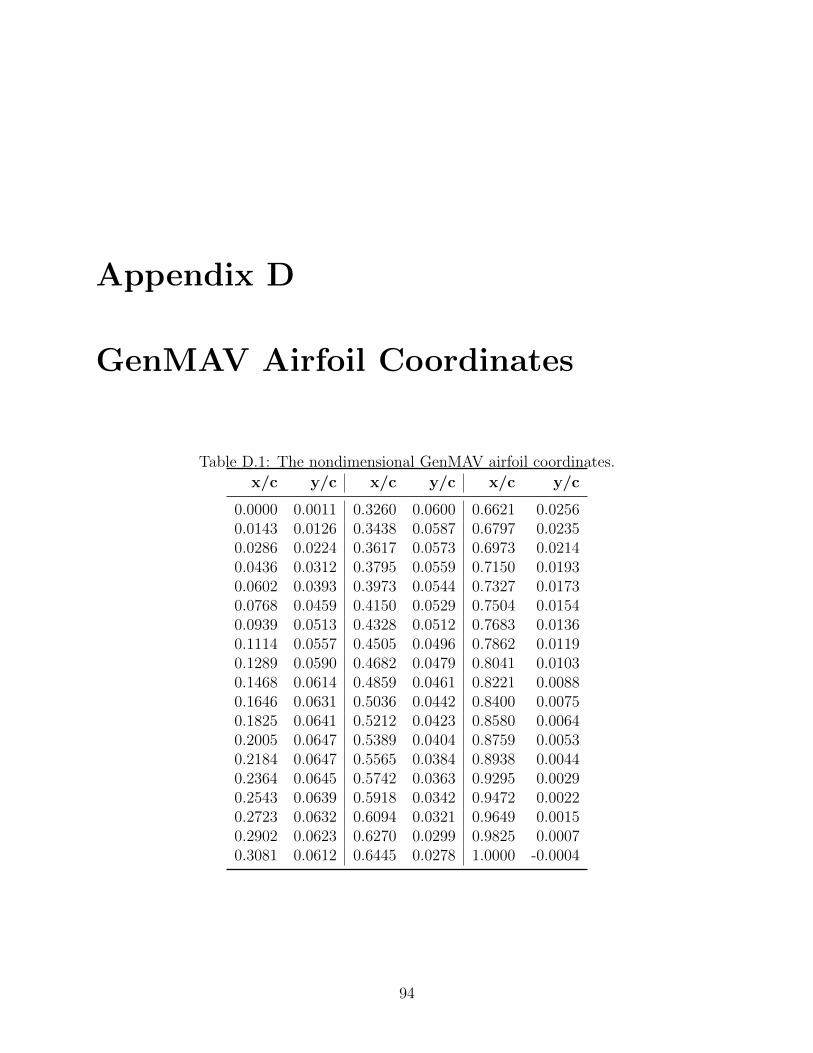
Appendix D
GenMAV Airfoil Coordinates
Table D.1: The nondimensional GenMAV airfoil coordinates.
x/c y/c x/c y/c x/c y/c
0.0000 0.0011 0.3260 0.0600 0.6621 0.02560.0143 0.0126 0.3438 0.0587 0.6797 0.02350.0286 0.0224 0.3617 0.0573 0.6973 0.02140.0436 0.0312 0.3795 0.0559 0.7150 0.01930.0602 0.0393 0.3973 0.0544 0.7327 0.01730.0768 0.0459 0.4150 0.0529 0.7504 0.01540.0939 0.0513 0.4328 0.0512 0.7683 0.01360.1114 0.0557 0.4505 0.0496 0.7862 0.01190.1289 0.0590 0.4682 0.0479 0.8041 0.01030.1468 0.0614 0.4859 0.0461 0.8221 0.00880.1646 0.0631 0.5036 0.0442 0.8400 0.00750.1825 0.0641 0.5212 0.0423 0.8580 0.00640.2005 0.0647 0.5389 0.0404 0.8759 0.00530.2184 0.0647 0.5565 0.0384 0.8938 0.00440.2364 0.0645 0.5742 0.0363 0.9295 0.00290.2543 0.0639 0.5918 0.0342 0.9472 0.00220.2723 0.0632 0.6094 0.0321 0.9649 0.00150.2902 0.0623 0.6270 0.0299 0.9825 0.00070.3081 0.0612 0.6445 0.0278 1.0000 -0.0004
94

Appendix E
Additional Wind Tunnel Testing
Details
E.1 Lift & Drag Coefficient Corrections
During wind tunnel testing, air flow around the airfoil models cannot perfectly represent
freestream characteristics. Realistic limitations on test section size prevent wall boundaries
from accuractely representing free air conditions. Barlow’s [39] correction method comes
from the method of images, where singularities are deliberately arranged to simulate real
wall boundaries in a flow field. This is a lead-in to the panel method, which predicts 2D ideal
flow fields around immersed geometries (same principle used by XFOIL). The coefficients
presented in this work use corrections derived from those concepts.
Cl = KCluClu Cd = KCduCdu (E.1)
where KClu and KCdu are the correction factors relating corrected and uncorrected lift and
drag coefficients, and “u” subscripts denote uncorrected values. Solid εsb and wake εwb
blockage factors account for the change in freestream flow speeds due the presence of the
physical model and its downstream wake, respectively.
KClu = 1− σ − 2εsb − 2εwb
95

KClu = 0.960− 0.357(Cdu) (E.2)
KCdu = 1− 3εsb − 2εwb
KCdu = 0.979− 0.357(Cdu) (E.3)
Compression of streamlines by the limited cross sectional test section area induces an increase
in lift. This is corrected by an adjustment to the effective angle of attack:
α = αu +57.3σ
2π
(clu + 4cm 1
4u
)α = αu + 0.239(clu) (E.4)
A reduction in effective airfoil span can arise from the boundary layer that generates along
the floor and ceiling of the test section. Recently, Bilgen [6] determined the boundary
layer displacement thickness at the airfoil quarter chord location as a function of static port
pressure. This did not exceed the finite gap between the spanwise airfoil edges and test
section surfaces, so its effect was assumed to be nominally zero.
96

E.2 Load Cell Calibrations
Two Transducer Techniques MLP-10 10 lb capacity load cells measure lift and drag forces.
Each is connected to a Transducer Techniques TMO signal conditioner. Sensor signals are
carried by shielded cabling to reduce interference noise. Individual load cell transfer functions
are arrived from simple in-situ experiments. Precision weights were connected to the load
cells via a high-gauge cable running through a low friction pulley. The C-arm attachment
point lies at the center span-quarter chord location, by using of a metal “calibration” bar in
place of the airfoil. The output trends demonstrate excellent linearity within the range of
expected forces.
y = -1.6720x + 0.6172 R² = 0.9998
-0.5
0.0
0.5
1.0
1.5
2.0
2.5
-1.2 -1 -0.8 -0.6 -0.4 -0.2 0 0.2 0.4 0.6
Forc
e (
N)
Voltage (V)
Lift LC Output
Linear (Lift LC Output)
y = -1.5190x + 1.0275 R² = 1.0000
0.0
0.2
0.4
0.6
0.8
1.0
1.2
1.4
1.6
-0.4 -0.2 0.0 0.2 0.4 0.6 0.8
Forc
e (
N)
Voltage (V)
Drag LC Output
Linear (Drag LC Output)
Figure E.1: Load cell output as a function of output voltage for lift (top) and drag (bottom).
97

E.3 Variation of WT Flow Speeds
0.00
0.05
0.10
0.15
0.20
0.25
0.30
0.35
0.40
0 2.5 5 7.5 10 12.5 15 17.5 20
Std
De
v o
f Fl
ow
Sp
ee
d
Flow Speed (m/s)
Variabilty of Flow Speed
Fan 1 ON
Fan 1+2 ON
Figure E.2: Standard deviation of flow speed measurements as a function of flow speed.
0
0.5
1
1.5
2
2.5
3
3.5
4
4.5
5
1 2 3 4 5 6 7 8 9 10 11 12 13 14 15 16 17 18 19 20 21 22 23
Flo
w S
pee
d (
m/s
)
Measurement #
U=2.5m/s, Highest Variability
Flow Speed
Mean + Std. Dev.
Mean - Std. Dev.
Figure E.3: Average wind tunnel speeds towards the lower limit of the flow speed range.
98

7.5
8
8.5
9
9.5
10
10.5
11
11.5
12
12.5
1 2 3 4 5 6 7 8 9 10 11 12 13 14 15 16 17 18 19 20 21 22 23
Flo
w S
pee
d (
m/s
)
Measurement #
U=10m/s, Lowest Variability
Flow Speed
Mean + Std. Dev.
Mean - Std. Dev.
Figure E.4: Average wind tunnel speeds around the middle of the flow speed range.
E.4 LCO Amplitude and Frequency Plots
The plot on the following pages were generated in support of analysis on the limit cycle os-
cillations discussed in Chapter 7. Note that actuation indicies 0 to 24 represent an actuation
sweep from 0%→ −100%→ +100%→ −100%→ 0%.
99

010
2030
010203040α=
−5
speed=9m/s
010
2030
010203040α=
0
010
2030
010203040α=
5
010
2030
010203040α=
10
010
2030
0102030α=
15
010
2030
0102030
speed=13m/s
010
2030
010203040
010
2030
0102030
010
2030
010203040
010
2030
0102030
010
2030
010203040
speed=17m/s
010
2030
010203040
010
2030
010203040
010
2030
0102030
010
2030
0102030
Note:Forallplots,abscissa
isfrequency
(hz),andordinate
isactuationindex
number.
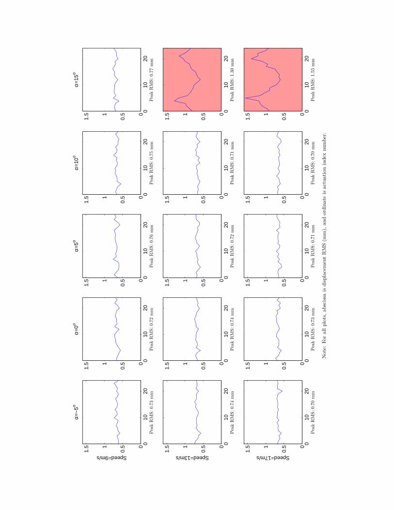
010
200
0.51
1.5
PeakRMS:0.73
mm
α=−
5o
Speed=9m/s
010
200
0.51
1.5
PeakRMS:0.72
mm
α=0o
010
200
0.51
1.5
PeakRMS:0.76
mm
α=5o
010
200
0.51
1.5
PeakRMS:0.75mm
α=10
o
010
200
0.51
1.5
PeakRMS:0.77
mm
α=15
o
010
200
0.51
1.5
PeakRMS:0.74
mm
Speed=13m/s
010
200
0.51
1.5
PeakRMS:0.74
mm
010
200
0.51
1.5
PeakRMS:0.72
mm
010
200
0.51
1.5
PeakRMS:0.71mm
010
200
0.51
1.5
PeakRMS:1.30
mm
010
200
0.51
1.5
PeakRMS:0.70
mm
Speed=17m/s
010
200
0.51
1.5
PeakRMS:0.73
mm
010
200
0.51
1.5
PeakRMS:0.71
mm
010
200
0.51
1.5
PeakRMS:0.70mm
010
200
0.51
1.5
PeakRMS:1.55
mm
Note:Forallplots,abscissa
isdisplacementRMS(m
m),
andordinate
isactuationindex
number.

E.5 Laser Displacement Plots
The output from the laser displacement sensor mounted on the wind tunnel test section wall
is plotted in Figure E.5. The laser is nominally aimed at the trailing edge of the airfoil during
all tests. These values are inherently inaccurate, due to the fixed mounting of the sensor and
movement of the airfoil. Consider the scenario that occurs for one particular actuation input
level. The laser may measure deflection at a different chordwise station along the airfoil for
a different attack angles.
102

−2000 −1000 0 1000 2000−15
−10
−5
0
5
10
15
Laser
Displacement(m
m)
V=9.0m
/s
−2000 −1000 0 1000 2000−15
−10
−5
0
5
10
15
LaserDisplacement(m
m)
V=13.0m/s
-5.0 deg.
-2.5 deg.
0.0 deg.
2.5 deg.
5.0 deg.
7.5 deg.
10.0 deg.
12.5 deg.
15.0 deg.
−2000 −1000 0 1000 2000−15
−10
−5
0
5
10
15
Laser
Displacement(m
m)
V=17
.0m/s
Figure E.5: Static displacements versus input voltage for flow speeds U = 9, 13, 17m/s.
103

Appendix F
Additional Lightweight Circuit Details
Two T-2505 and one T-1505 AM Power Systems DC-DC converters provide the voltage
amplification for the MFC actuators. The total bleed resistance is divided amongst multiple
medium power (1W) resistors, to prevent over-volting. Three out of the four op amp (Digikey
part OPA4743UA/2K5) channels are connected to a general purpose NPN power transistor
(Digikey part 497-2462-1) to uncouple current draw from the signal source. The high voltage
diodes were samples from HVCA (part SP5L).
CAM files are generated and sent to Advanced Circuits, Aurora, CO, which handles printed
circuit board manufacture. The two layer board is then populated in-house almost exclusively
with SMDs using a Hakko hot air rework station.
After the PCB was populated, a few issues such as an insufficient solder pad size became
apparent. These were resolved after a few light modifications. Since flight weight is a concern,
the weight of the PCB was examined. The total weight was mostly represented by the three
converters (4.5 g each), and the PCB (19 g), for a total of 32.5 g. A 9 V battery weighs
about 47 g by comparison. A more complete breakdown of typical components used with a
2 lb MAV are compared in Chapter 4.
104

AO1+
DO1+
T1505 T2505T2505
PWR IN-O
UT
-OU
T
+OU
T+O
UT
-IN-IN
+IN
+IN
-OU
T-O
UT
+OU
T+O
UT
-IN-IN
+IN
+IN
-OU
T-O
UT
+OU
T+O
UT
-IN-IN
+IN
+IN
D1
D2
D3
R7
R8
R9
R19
R20
R21
C4
B1
E3
C4
B1
E3
C4
B1
E3
R11
R12
R13
R14
R15
R16
R17
R18
R22
R23
R10
1
32
4
JST1
C1
R4
C3
R5
C5
R6
2
31
IC1A
6
57
IC1B
9
108
IC1C
13
1214
IC1D
411R
1
R2
R3
C7
MFC2-2
MFC2-1
MFC1-2
MFC1-1
AO2+
AO2+
VIN
1
VIN1
VIN
2
VIN2
VIN
3
VIN3
DO1 DO1
VIN
VIN
2.45V2
Figure F.1: Electrical schematic of the lightweight MFC driver PCB.
Figure F.2: Final populated revision 1 of the lightweight circuit prototype.
105