Embed Size (px)
Citation preview
DESIGN OPTIMIZATION OF PERIODIC FLOWS USING A
TIME-SPECTRAL DISCRETE ADJOINT METHOD
A DISSERTATION
SUBMITTED TO THE DEPARTMENT OF AERONAUTICS &
ASTRONAUTICS
AND THE COMMITTEE ON GRADUATE STUDIES
OF STANFORD UNIVERSITY
IN PARTIAL FULFILLMENT OF THE REQUIREMENTS
FOR THE DEGREE OF
DOCTOR OF PHILOSOPHY
Ki Hwan Lee
June, 2010

http://creativecommons.org/licenses/by-nc/3.0/us/
This dissertation is online at: http://purl.stanford.edu/zf671jy0354
© 2010 by Ki Hwan Lee. All Rights Reserved.
Re-distributed by Stanford University under license with the author.
This work is licensed under a Creative Commons Attribution-Noncommercial 3.0 United States License.
ii

I certify that I have read this dissertation and that, in my opinion, it is fully adequatein scope and quality as a dissertation for the degree of Doctor of Philosophy.
Juan Alonso, Primary Adviser
I certify that I have read this dissertation and that, in my opinion, it is fully adequatein scope and quality as a dissertation for the degree of Doctor of Philosophy.
Antony Jameson
I certify that I have read this dissertation and that, in my opinion, it is fully adequatein scope and quality as a dissertation for the degree of Doctor of Philosophy.
Robert MacCormack
Approved for the Stanford University Committee on Graduate Studies.
Patricia J. Gumport, Vice Provost Graduate Education
This signature page was generated electronically upon submission of this dissertation in electronic format. An original signed hard copy of the signature page is on file inUniversity Archives.
iii
Abstract
Standard methods for unsteady optimization carry heavy computational costs and
large storage requirements, mostly due to the lengthy time integration involved in
the unsteady flow simulations. Such difficulties limit its practical application to cases
where the time integration is performed over only a smaller segment of the entire
period. The result is a loss of accuracy in the representation of the physical model.
For certain unsteady flows with periodicity, a dramatic reduction in both compu-
tational cost and required storage is realized through implementing the Time Spectral
method. Furthermore, by introducing an adjoint-based method as an alternative way
of obtaining gradient information, computational cost is further reduced. This combi-
nation of Time-Spectral and adjoint-based methodology therefore allows for unsteady
optimization within a reasonable time frame while maintaining accuracy.
In this dissertation, the Discrete Adjoint method is implemented and applied to
unsteady flows with periodicity, in the context of the Time Spectral Method. The
acquired adjoint gradient information is fed into an optimizer and truly unsteady
optimization work is carried out for the first time on a realistic test case. The devel-
opment and implementation of necessary boundary conditions prove crucial for the
successful implementation of the Discrete Adjoint method.
As a simple test case, the NACA 0012 airfoil is selected for simulation in steady
inviscid, unsteady inviscid, steady viscous, and unsteady viscous flows. In each case,
the resulting gradient information obtained from both the adjoint and finite difference
method is compared. Upon completion of the airfoil test case, the adjoint-based
method is applied to a helicopter blades, UH60, for both steady and unstaedy inviscid
flows. The gradient information obtained by the adjoint-based method shows good
iv
agreement with the conventional, Finite Difference gradient information.
The design methodology was developed for a single processor, however, multi-
processor capability is also implemented. In order to accommodate realistic meshes,
multi-block capability is added as well. With all of the necessary components im-
plemented, optimization is carried out on the UH60 helicopter blade. The objective
function is time-averaged torque over all time instances and the optimized result
shows an improvement of 5 % over the current configuration. Stanford University
Multi-block (SUmb), while implementing the unsteady Reynolds-Averaged Navier
Stokes equations with multi-block and multi-processor algorithms, is the chosen flow
solver. PETSc is employed as the adjoint solver.
Successful implementation of the Discrete Adjoint method to unsteady fluids with
periodicity provides the gradient information more easilty than the traditional finite
difference method which is hindered by its heavy computational cost and large stor-
age requirements. This research establishes a new optimization methodology which
utilizes Discrete Adjoint gradient information derived from flow solutions, obtained
using the Time Spectral method.
v
Acknowledgements
This research has been made possible by the ASC project funded by the Department
of Defense and their dedication to set up an infrastructure for massively parallel
computation.
I would like to express my deep gratitude to Professor Alonso, my advisor, for
providing me the opportunity to work in this interesting field of research and for his
continual support and guidance, encouragement, and numerous intangibles through-
out the research. I also would like to thank Professor Jameson, who pioneered the
use of adjoint-based methods in Aerospace engineering, for his valuable insight in the
the subject and his inputs.
All of my friends at Stanford supported me by enriching my life. Their valuable
insight in the research also helped me to achieve my goal. My family members has
been essential in carrying me up to this point of my life. Without them, nothing
would have been possible.
vi
Contents
Abstract iv
Acknowledgements vi
1 Introduction 1
1.1 Introduction to Research . . . . . . . . . . . . . . . . . . . . . . . . . 1
1.2 Gradient Based Optimization . . . . . . . . . . . . . . . . . . . . . . 3
1.3 Adjoint Gradient Calculation . . . . . . . . . . . . . . . . . . . . . . 4
1.4 Time Spectral Method . . . . . . . . . . . . . . . . . . . . . . . . . . 5
1.5 Goals of Research: Time Spectral Adjoint
Method . . . . . . . . . . . . . . . . . . . . . . . . . . . . . . . . . . 6
1.6 Applications of the Time Spectral Adjoint
Method . . . . . . . . . . . . . . . . . . . . . . . . . . . . . . . . . . 7
2 Governing Equations 10
2.1 Navier-Stokes Equations and RANS . . . . . . . . . . . . . . . . . . . 10
2.2 Euler Equations . . . . . . . . . . . . . . . . . . . . . . . . . . . . . . 12
3 Development of A Time-Spectral Discrete Adjoint Solver 16
3.1 Benefits of Time-Spectral Discrete Adjoint
Method . . . . . . . . . . . . . . . . . . . . . . . . . . . . . . . . . . 16
3.2 Flow Solver . . . . . . . . . . . . . . . . . . . . . . . . . . . . . . . . 18
3.2.1 Time Spectral Method . . . . . . . . . . . . . . . . . . . . . . 18
3.2.2 URANS Flow Solver . . . . . . . . . . . . . . . . . . . . . . . 20
vii
3.3 Discrete Adjoint Solver . . . . . . . . . . . . . . . . . . . . . . . . . . 23
3.3.1 Discrete vs. Continuous Adjoint . . . . . . . . . . . . . . . . . 23
3.3.2 General Derivation of the Adjoint Equation . . . . . . . . . . 25
3.3.3 Implementation . . . . . . . . . . . . . . . . . . . . . . . . . . 26
3.3.4 Derivatives of the Time-Spectral Terms . . . . . . . . . . . . . 30
3.3.5 Inviscid Formulation . . . . . . . . . . . . . . . . . . . . . . . 32
3.3.6 Viscous Formulation . . . . . . . . . . . . . . . . . . . . . . . 44
3.3.7 Boundary Conditions . . . . . . . . . . . . . . . . . . . . . . . 50
3.3.8 Unsteady Boundary Conditions . . . . . . . . . . . . . . . . . 70
3.3.9 Multiblock/Multiprocessor Implementation Issues . . . . . . . 72
3.4 Optimization . . . . . . . . . . . . . . . . . . . . . . . . . . . . . . . 76
3.4.1 Hick-Henne Bump Functions . . . . . . . . . . . . . . . . . . . 76
3.4.2 Implementation Using a Gradient Based Optimizer
with Adjoint Gradients . . . . . . . . . . . . . . . . . . . . . . 78
4 Results 81
4.1 Description of the Test Cases . . . . . . . . . . . . . . . . . . . . . . 81
4.1.1 NACA 0012 Airfoil Mesh . . . . . . . . . . . . . . . . . . . . . 82
4.1.2 UH60 Helicopter Rotor Mesh . . . . . . . . . . . . . . . . . . 85
4.1.3 Flat Channel Mesh . . . . . . . . . . . . . . . . . . . . . . . . 87
4.2 Verification of Inviscid Gradients . . . . . . . . . . . . . . . . . . . . 88
4.2.1 Steady Gradient Comparison . . . . . . . . . . . . . . . . . . 89
4.2.2 Unsteady . . . . . . . . . . . . . . . . . . . . . . . . . . . . . 89
4.2.3 Multiblock . . . . . . . . . . . . . . . . . . . . . . . . . . . . . 94
4.3 Verification of Viscous Gradients . . . . . . . . . . . . . . . . . . . . 96
4.4 Adjoint Solver Performance Analysis . . . . . . . . . . . . . . . . . . 100
4.5 Optimization of the UH60 Rotor . . . . . . . . . . . . . . . . . . . . . 103
4.5.1 Description . . . . . . . . . . . . . . . . . . . . . . . . . . . . 103
4.5.2 CFD/CSD Analysis . . . . . . . . . . . . . . . . . . . . . . . . 104
4.5.3 Optimization Results . . . . . . . . . . . . . . . . . . . . . . . 105
viii
5 Conclusions & Future Work 117
5.1 Conclusions . . . . . . . . . . . . . . . . . . . . . . . . . . . . . . . . 117
5.2 Future Work . . . . . . . . . . . . . . . . . . . . . . . . . . . . . . . . 120
A Optimization 121
A.1 Linear Programming . . . . . . . . . . . . . . . . . . . . . . . . . . . 121
A.2 Nonlinear Programming . . . . . . . . . . . . . . . . . . . . . . . . . 124
Bibliography 127
ix
List of Tables
4.1 Summary Table of Test Cases . . . . . . . . . . . . . . . . . . . . . . 82
4.2 Summary Table of Applications . . . . . . . . . . . . . . . . . . . . . 82
4.3 Convergence comparison between the original and modified meshes . 94
4.4 Accuracy of Time Spectral Adjoint Method on NACA 0012
- Viscous Flow/Adjoint . . . . . . . . . . . . . . . . . . . . . . . . . . 99
4.5 Design parameters and two set of nonlinear constraints . . . . . . . . 107
4.6 UH60 blade optimization with no trim angle constraints . . . . . . . 108
4.7 Design parameters and four sets of constraints . . . . . . . . . . . . . 110
4.8 UH60 blade optimization with four sets of constraints . . . . . . . . . 111
4.9 Computational time comparison for the inviscid UH60 test case . . . 115
4.10 Computational time comparison for viscous calculations on a NACA
0012 . . . . . . . . . . . . . . . . . . . . . . . . . . . . . . . . . . . . 116
x
List of Figures
1.1 Optimization Process Schematics . . . . . . . . . . . . . . . . . . . . 8
2.1 Boundary Layer Thickness . . . . . . . . . . . . . . . . . . . . . . . . 14
3.1 Flux Discretization in 2 D . . . . . . . . . . . . . . . . . . . . . . . . 27
3.2 Cell Types . . . . . . . . . . . . . . . . . . . . . . . . . . . . . . . . . 28
3.3 Flux Discretization in 2 D . . . . . . . . . . . . . . . . . . . . . . . . 33
3.4 Inviscid Flux Discretization in Three-dimensions . . . . . . . . . . . . 36
3.5 Artificial Dissipation Discretization in Two-dimensions . . . . . . . . 37
3.6 Artificial Dissipation Discretization in Matrix . . . . . . . . . . . . . 41
3.7 Stencil depicting the required cells for inviscid flux and artifical dissi-
pation calculations . . . . . . . . . . . . . . . . . . . . . . . . . . . . 43
3.8 Viscous Flux in 3D . . . . . . . . . . . . . . . . . . . . . . . . . . . . 46
3.9 Imaginary Box for Nodal Value . . . . . . . . . . . . . . . . . . . . . 47
3.10 Average Nodal Value . . . . . . . . . . . . . . . . . . . . . . . . . . . 48
3.11 Surface Calculation . . . . . . . . . . . . . . . . . . . . . . . . . . . . 49
3.12 Stencil for the viscous flux, inviscid flux and artificial dissipation cal-
culations . . . . . . . . . . . . . . . . . . . . . . . . . . . . . . . . . . 51
3.13 Supersonic Inlet . . . . . . . . . . . . . . . . . . . . . . . . . . . . . . 53
3.14 Supersonic Outlet . . . . . . . . . . . . . . . . . . . . . . . . . . . . . 53
3.15 Euler Boundary . . . . . . . . . . . . . . . . . . . . . . . . . . . . . . 54
3.16 Euler Boundary – Pressure Extrapolation . . . . . . . . . . . . . . . 54
3.17 Viscous Boundary . . . . . . . . . . . . . . . . . . . . . . . . . . . . 56
3.18 Symmetric Boundary . . . . . . . . . . . . . . . . . . . . . . . . . . . 56
xi
3.19 Farfield Boundary . . . . . . . . . . . . . . . . . . . . . . . . . . . . . 57
3.20 Multiblock Mesh Configuration . . . . . . . . . . . . . . . . . . . . . 73
3.21 Mutiblock With Halo Cell . . . . . . . . . . . . . . . . . . . . . . . . 73
3.22 Multiblock With Corresponding Jacobian . . . . . . . . . . . . . . . . 74
3.23 Multiblock Horizontal Halo Exchange . . . . . . . . . . . . . . . . . . 75
3.24 Multiblock Vertical Halo Exchange . . . . . . . . . . . . . . . . . . . 75
3.25 Hicks-Henne perturbation function . . . . . . . . . . . . . . . . . . . 77
3.26 UH60 airfoil section with applied Hicks-Henne perturbation function . 78
4.1 NACA 0012 Airfoil Mesh . . . . . . . . . . . . . . . . . . . . . . . . . 83
4.2 NACA 0012 Single Block Mesh . . . . . . . . . . . . . . . . . . . . . 84
4.3 Comparison of Single and Multiblock Topologies for the NACA 0012
Mesh . . . . . . . . . . . . . . . . . . . . . . . . . . . . . . . . . . . . 84
4.4 UH60 Helicopter Blade Mesh . . . . . . . . . . . . . . . . . . . . . . 85
4.5 UH60 Modified Mesh . . . . . . . . . . . . . . . . . . . . . . . . . . . 86
4.6 Viscous Flat Channel Mesh . . . . . . . . . . . . . . . . . . . . . . . 87
4.7 Inviscid, Steady Gradient Comparison for the NACA 0012 . . . . . . 89
4.8 Sensitivity comparison for angular frequency = 5 . . . . . . . . . . . 90
4.9 Sensitivity comparison for angular frequency = 35 . . . . . . . . . . . 91
4.10 Sensitivity comparison for angular frequency = 140 . . . . . . . . . . 92
4.11 Inviscid, Unsteadiness Sensitivity Captured with Time Spectral Dis-
crete Adjoint Method . . . . . . . . . . . . . . . . . . . . . . . . . . . 93
4.12 Time Spectral Adjoint Gradient Comparison for the UH60 . . . . . . 94
4.13 Arbitrary Multi-Block Halo Cells . . . . . . . . . . . . . . . . . . . . 95
4.14 Multi-Block Adjoint Solver Study . . . . . . . . . . . . . . . . . . . . 96
4.15 Viscous Flat Channel Sensitivity Study . . . . . . . . . . . . . . . . . 97
4.16 NACA Airfoil 121 × 33 × 13 mesh . . . . . . . . . . . . . . . . . . . . 97
4.17 Viscous NACA Airfoil Mesh Refinement Study . . . . . . . . . . . . . 98
4.18 NACA Airfoil Time Spectral Adjoint Sensitivity Comparison . . . . . 99
4.19 Time Spectral Discrete Adjoint run on UH60 Mesh, part 1 . . . . . . 100
4.20 Time Spectral Discrete Adjoint run on UH60 Mesh, part 2 . . . . . . 101
xii
4.21 Modified CFD/CSD Analysis Diagram . . . . . . . . . . . . . . . . . 105
4.22 UH60 base and optimized configurations . . . . . . . . . . . . . . . . 106
4.23 Cp plots at different radial locations . . . . . . . . . . . . . . . . . . . 108
4.24 Geometric changes along the radial span . . . . . . . . . . . . . . . . 109
4.25 Optimized geometry with full trim constraints . . . . . . . . . . . . . 111
4.26 Geometric changes along the radial span with full trim constrants . . 112
4.27 Cp plot comparison at different radial locations
with full trim constraints . . . . . . . . . . . . . . . . . . . . . . . . . 113
xiii
Chapter 1
Introduction
1.1 Introduction to Research
Shape optimization is an important part of engineering design and manufacturing. In
aerospace engineering, shape optimization is particularly important because geometry
holds a great influence over the overall performance and stability of the aircraft.
Traditionally, optimization is performed based on the experience and intuition of the
engineer.
Typical objective functions in aerospace engineering have complicated dependence
relatioinships due to the nonlinear interaction of many input variables. Hence, rea-
sonable ways to approach optimization problems are either heavily dependent on the
judgement of experienced eyes or based on reduced models for which a set of analytical
solutions exist.
Recent developments[42, 55, 35, 53, 49, 12, 57, 19, 37, 56, 45, 46] in Numerical
Science facilitate the use of Computational Fluid Dynamics (CFD) in aerodynamic
shape optimization, and accordingly, significant performance improvements have been
achieved. However, most of this work has been confined to steady cases or unsteady
cases using vastly simplified models. The objective of the present work is to develop
a high-order shape optimization method for unsteady flow.
Although the computer industry has made remarkable technological leaps in recent
years, accurate resolution of unsteady fluid phenomena still requires a prohibitively
1
CHAPTER 1. INTRODUCTION 2
large amount of computing power. In addition, the large number of design parameters
used in the optimization can become an additional hindrance. In order to estimate
the gradient with respect to each parameters by the finite difference method, the
process of solving the set of governing equations must be repeated a number of times
equal to the number of independent parameters as will be discussed in the following
sections. An adjoint-based method for determining gradients[24, 50] can obviate this
process, requiring additional computational cost equivalent to only a flow solution.
As a result, the time savings with the adjoint-based gradients is proportional to the
number of independent parameters used in the optimization.
Even with the incorporation of adjoint-based gradients, the unsteady solution still
often requires a large number of time steps for a reasonably accurate representation
of the unsteady flow phenomena. It is not unusual to require 1,000 to 100,000 time
steps of unsteady integration, depending on the nature of the flow being considered.
In addition to the CPU time, the large amount of time spent storing the entire flow
solution history make this approach practically infeasible to implement. In order to
alleviate these costs, the Time-Spectral Method for unsteady flow solutions has been
adopted in this research.
Employing the Time Spectral Method[10] together with the Discrete Adjoint for-
mulation for gradient information yields the following advantages:
• Reduction in the computational costs for flow solutions at each design iteration
• Reduction in the computational costs for determining gradients at each design
iteration
• Ability to optimize with a large number of design parameters
• Provision of error estimation[5] information for unsteady flows (as a by-product
of solving the adjoint equations).
Recent works by Nadarajah and Tatossian[45, 46] describe parallel efforts to reduce
the cost of unsteady shape optimization using the nonlinear frequency domain method
in adjoint approach.
CHAPTER 1. INTRODUCTION 3
In this work, after implementing and verifying all of these necessary components,
optimization has been performed on a helicopter rotor to verify the new adjoint
gradient-based, unsteady optimization methodology. In the following sections, the
background and objectives of the research are discussed more extensively.
1.2 Gradient Based Optimization
Before computational methods were used in the design process, the primary tool for
the development of aerodynamic configurations was the wind tunnel. With the tech-
nological advances in both computer and numerical science, computational methods
are now widely accepted in the aircraft industry. Much of the early effort was made
by Murman and Cole[42], Jameson[17, 19] and Caughey[27], to name a few, although
advancements have been pursued throughout the years. Even though the introduc-
tion of computational methods for shape optimization was widely recognized as an
idea with great potential, the computational cost for design work posed a formidable
challenge.
Gradient-based optimization[20], by nature, requires evaluation of the objective
and constraint functions and their gradients at each design iteration. Suppose the
cost function depends on N parameters.
I = I(α1, α2, · · · , αN)
A direct approach to evaluating the gradients is to perturb each parameter in turn,
recalculate the cost, and use finite differences to estimate the gradient.
∂I
∂αi
=I(α1, · · · , αi + δαi, · · · , αN) − I(α1, · · · , αi, · · · , αN)
δαi
Consequently, the cost of finding a descent direction at each design iteration, when
using finite differences to compute the necessary gradients, is equivalent to
(N + 1) ∗ Tflow,
CHAPTER 1. INTRODUCTION 4
where N is the number of design parameters and Tflow is the time required to solve
the flow equations and evaluate the objective and constraint functions. Considering
that a viscous solution on a medium sized mesh for a three dimensional wing costs
approximately 5 hours of CPU time, the total time to find a descent direction at each
design iteration would take more than 100 CPU hours for 20 design parameters.
1.3 Adjoint Gradient Calculation
While the introduction of new computational tools presented a new method for op-
timization, its practical application is limited by the manageability of the problem
size. As discussed in the previous section, obtaining gradient information for each
parameter at every design iteration is very time consuming. Assuming a quadratic
behavior of the objective function and constraints, a Sequential Quadratic Program-
ming algorithm[9, 48] will find its optimum after a number of iterations equal to the
number of design parameters. Assuming N parameters, it will require at least N2
evaluations of the flow solution if the gradients are calculated by finite differences.
This proves to be a serious bottleneck in the optimization process, particularly for
design problems with a large N .
In 1988, Jameson successfully introduced a concept of control theory into the field
of aerodynamic shape optimization[20]. The crux of this idea is to use control theory
in order to obtain gradients for every parameter at each design iteration at a cost
equivalent to capturing a single flow solution. The significance of this method is that,
at each design iteration, the computational time required to determine a descent
direction is of the same order as the time required to evaluate one flow solution.
Instead of requiring N2 evaluations, a time equivalent to N evaluations of the flow
solution would suffice to attain an optimal point in the ideal case. The method is
termed the Adjoint Method.
Following earlier applicatioins of this approach to airfoil and wing design [24,
26, 50, 51, 28], Kim[33] applied a continuous adjoint formulation for aerodynamic
CHAPTER 1. INTRODUCTION 5
shape optimization to multi-element airfoils, using the compressible Reynolds Aver-
aged Navier-Stokes equations. Drag minimization and lift maximization were per-
formed on multi-element airfoils using a multi-block, multi-processor RANS solver.
As design variables, Kim chose the airfoil shape, element configuration and angle
of attack. In his work, the application of the Adjoint Method to the compressible
RANS equation was demonstrated successfully in the aerodynamic shape optimiza-
tion of high lift systems.
Nadarajah[47] compared a continuous and a discrete Adjoint formulation. The
difference between these two formulations is in the way of applying control theory
directly to the actual discretized form of the governing equation. He also applied the
discrete Adjoint Method to the inverse problem in which both drag minimization and
reduced near field pressure minimization were achieved.
1.4 Time Spectral Method
In order to reduce the inherently large computational costs, more efficient ways of
solving unsteady flows have garnered much attention. One approach is the Harmonic
Balance Method by Hall[58]. Another is the Non-Linear Frequency Domain (NLFD)
method developed by McMullen[40]. This takes a pseudo-spectral approach to recast
the non-linear, unsteady equations in the time domain into an equivalent set of equa-
tions in the frequency domain. Once in the frequency domain, only the number of
modes used to approximate the solution matters. Selecting a finite number of modes
represents a loss of information. However, McMullen shows by using NLFD methods
that the first few modes are often sufficient to approximate an unsteady solution with
reasonable accuracy.
Although the advantages of the NLFD method are significant, it incurs an addi-
tional cost of computing Fourier transforms to the frequency domain and the inverse
Fourier transform to the time domain. Not only does the additional source of com-
putational cost slightly offset its advantages, it requires an additional set of complex
variables which causes extra complexity in the code and demands more storage space.
More specifically, it is equivalent to decreasing the available memory by half. Even
CHAPTER 1. INTRODUCTION 6
with these drawbacks, the NLFD method by McMullen opened up the possibility of
incorporating spectral solution approaches for periodic unsteady flows.
As an alternative, Gopinath[11], Jameson, and Van der Weide proposed the Time
Spectral Method. The Time Spectral Method utilizes a clever formulation of the time
derivative terms in the time domain which captures the effect of the spectral solution.
Typical approaches for evaluating time derivatives use two or more time instances of
the solution that had been previously computed. The Backward Difference Formula
(BDF) scheme is one such approach that uses three time instances of the solutions and
is second order accurate in time. However, the Time Spectral method makes use of all
time instances, and it is this set of previously known solutions which contributes to
capturing the spectral effect. By cleverly exploiting the concept of a geometric series,
the final form of the derived equation hides all details of Fourier and inverse Fourier
transforms such that the use of complex variables is not necessary. Thus, it solves the
two difficulties in using the NLFD method. First, no additional computational cost
is required. Second, no additional memory is required. Hence, the Time Spectral
method achieves a better performance with lower CPU costs and smaller memory
requirements.
1.5 Goals of Research: Time Spectral Adjoint
Method
The application of the Adjoint Method to unsteady flow has been attempted previ-
ously by Nadarajah[45, 46, 47]. In Nadarajah’s work, in order to obtain time-accurate
unsteady gradients, unsteady adjoint equations were constructed at every time step
by using flow solutions around the current time step. Because obtaining the time-
accurate solution for unsteady flows can easily require thousands of time steps, the
unsteady adjoint equations must also be constructed and solved for the same large
number of time steps at each design iteration. Knowing that a Sequential Quadratic
Programming (SQP) algorithm[48] requires a number of iterations equivalent to the
number of design parameters to find an optimum, Nadarajah’s approach leaves no
CHAPTER 1. INTRODUCTION 7
choice but to either employ reduced order models or sacrifice the integrity of the un-
steady flow solution. Another serious bottleneck is due to storing unsteady solutions
at every time step. For example, assuming it takes about 10,000 time steps in order
to obtain unsteady solutions within the desired accuracy and the size of each solution
file is 20 MBytes, storing all of the solution would require 10,000 times 20 MBytes,
which is 200 GBytes. In a more realistic case, not only would storage space much
larger than 200 GBytes to be required, but also the input and output of that much
data renders the whole procedure unrealistic. It is well known both in theory and
in practice that I/O time, not CPU time, is the biggest bottleneck of computational
works.
The Time Spectral Adjoint Method, which combines the Time Spectral Method
and the Adjoint Method, can provide a viable solution to the unsteady design prob-
lem. The Time Spectral Adjoint Method can be applied to any unsteady flow with
periodicity to obtain unsteady gradients at the desired design iterations. As previ-
ously discussed, a successful implementation of this method would not only reduce
the convergence time of the unsteady flow solution, it would also deliver gradient
information for each design iteration at a computational cost equivalent to a single
additional time-spectral flow solution.
In the implementation of the Time Spectral Discrete Adjoint Method, all neces-
sary adjoint derivations are developed for both the Euler and Navier-Stokes equations,
along with different boundary conditions. In the multi-block, multi-processor imple-
mentation for the helicopter blade, a way of updating halo cells has been devised and
presented in the papers by the present author[34], [2], [1].
1.6 Applications of the Time Spectral Adjoint
Method
For initial inviscid test cases, a NACA 0012 airfoil configuration is chosen for simu-
lations in both steady and unsteady flow for a more practical application, a model of
the UH-60 helicopter rotor is chosen. Unsteady flow calculations are performed and
CHAPTER 1. INTRODUCTION 8
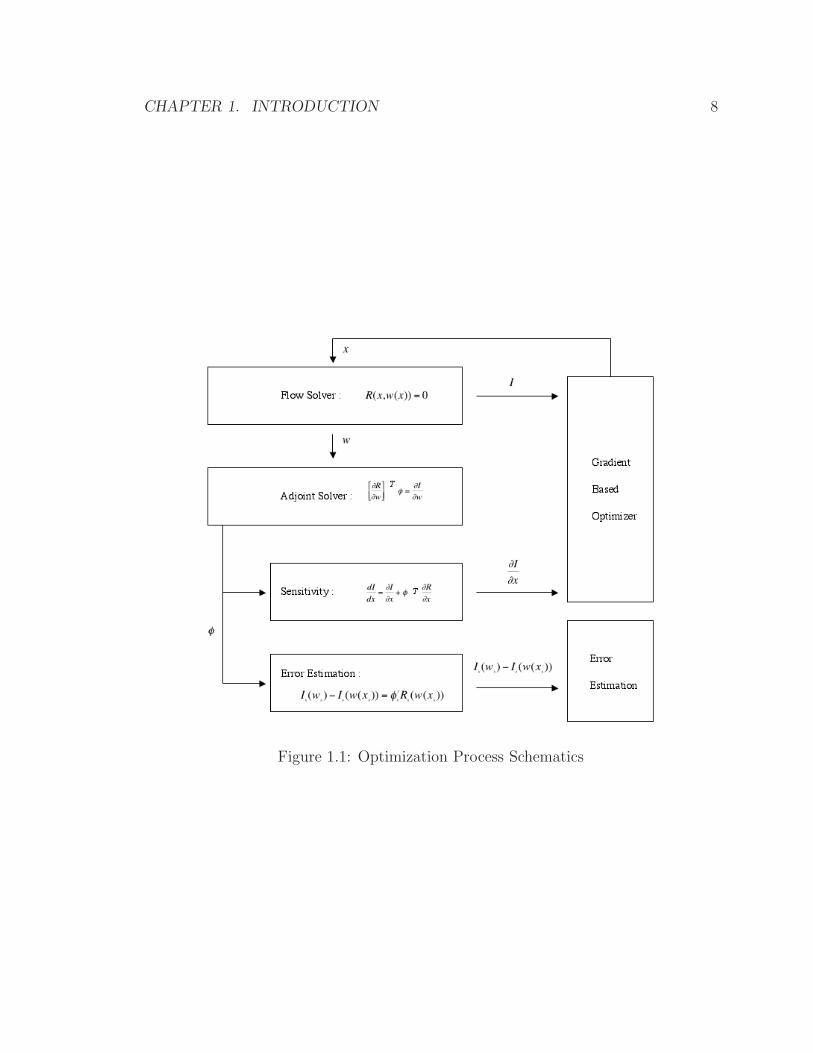
Figure 1.1: Optimization Process Schematics
CHAPTER 1. INTRODUCTION 9
once the gradient information obtained by the Adjoint Method is verified in compar-
ison with finite differences, it can be applied in the optimization process outlined in
figure 1.1
For the calculation of the flow solution, the Euler and Reynolds-Averaged Navier-
Stokes (RANS) solver is used. The solver, named SUmb, is multi-block and multi-
processor capable and utilizes implicit residual averaging, dual time stepping and
enthalpy damping convergence acceleration techniques. It also has a full implemen-
tation of the time-spectral formulation of Gopinath that is used in this research. For
the solution of the time-spectral adjoint system, the Portable, Extensible Toolkit for
Scientific Computation (PETSc), developed by Argonne National Laboratory is em-
ployed. A discrete adjoint formulation is applied, which offers a distinct advantage
in that there is no limitation in the choice of cost function. With the continuous
adjoint approach, the only available choice for the cost function are those functions
that explicitly depends on pressure or shear stress alone. For multi-processor imple-
mentation, MPI and MPI2 standard is used.
The drag coefficient is the chosen objective function for the steady case, and a
total drag coefficient over all the time instances of the time-spectral solution is chosen
for the unsteady case. For the helicopter blade, a torque is chosen with nonlinear
constraints on thrust and drag forces. Refere to 4.5 for more details.
Chapter 2
Governing Equations
2.1 Navier-Stokes Equations and RANS
The Navier-Stokes equations encompass the necessary physics for modeling the com-
pressible and viscous nature of a fluid. The three-dimensional Navier-Stokes equations
[14, 15, 36] can be written in indicial notation as,
∂w
∂t+∂fi
∂xi
=∂fvi
∂xi
, (2.1)
where the state vector w, inviscid flux vector f , and viscous flux fv are represented
by
w =
ρ
ρu1
ρu2
ρu3
ρE
, fi =
ρui
ρuiu1 + pδi1
ρuiu2 + pδi2
ρuiu3 + pδi3
ρuiH
, fvi =
0
σijδj1
σijδj2
σijδj3
ujσij + k ∂T∂xi
.
The viscous stress tensor, σ, can be written as
σij = µ
(
∂ui
∂xj
+ λδij∂uk
∂xk
)
,
10
CHAPTER 2. GOVERNING EQUATIONS 11
with µ, λ, and δ as the first and second coefficients of viscosity and the Kronecker delta
function, respectively. The coefficient of thermal conductivity, k, can be calculated
from the following relationship,
k =cpµ
Pr,
where Pr is the Prandtl number and cp is the specific heat at a pressure given by
p = (γ − 1)ρ
E −1
2(uiuj)
Temperature can be determined using the perfect gas law as,
T =P
Rρ.
A relationship between energy and enthalpy is
ρH = ρE + p,
where γ is the ratio of specific heats. E and H represent the total energy, the
stagnation enthalpy, respectively.
When applying the Navier-Stokes equations to physical engineering problems, a
transformation between the physical and computational coordinate systems (xi and
ξi) is desired. This transformation can be described using
Kij =
[
∂xi
∂ξj
]
, J = det(K), K−1ij =
[
∂ξi
∂xj
]
and
S = JK−1.
The elements of the matrix S are nothing but the face area of the given cell projected
into the x1, x2 and x3 directions in the finite volume formulation. Using the above
relationships and the physical observation that the sum of the projected face area
in each direction becomes zero in each cell, the Navier-Stokes equations[43] in the
CHAPTER 2. GOVERNING EQUATIONS 12
computational coordinate system become
∂Jw
∂t+∂Fi − Fvi
∂ξi= 0, (2.2)
where the inviscid and viscous flux contributions are now defined with respect to the
computational cell faces given by Fi = Sijfj and Fvi = Sijfvj .
To ensure numerical stability, artificial dissipation is added. The artificial dissipa-
tion scheme used in this research is a blended first and third order flux which was first
introduced by Jameson, Schmidt, and Turkel [22, 23, 29]. The artificial dissipation is
defined as
Di+ 1
2,j = ǫ2
i+ 1
2,j(wi+1,j − wi,j) − ǫ4
i+ 1
2,j(wi+2,j − 3wi+1,j + 3wi,j − wi−1,j). (2.3)
The first term in the above equation is a first order scalar diffusion term, where ǫ2i+ 1
2,j
is scaled by the normalized pressure difference and serves to damp oscillations near
shock waves. ǫ4i+ 1
2,j
is the coefficient for the third derivative of the artificial dissipation
flux. The coefficient is scaled so that it is zero in regions with large gradient, such as
shock waves.
2.2 Euler Equations
The three-dimensional Euler equations[14, 15, 36] can be written as,
∂w
∂t+∂fi
∂xi
= 0, (2.4)
where the state vector w and inviscid flux vector are represented by
w =
ρ
ρu1
ρu2
ρu3
ρE
, fi =
ρui
ρuiu1 + pδi1
ρuiu2 + pδi2
ρuiu3 + pδi3
ρuiH
.
CHAPTER 2. GOVERNING EQUATIONS 13
A relationship for calculating pressure, p, is given by
p = (γ − 1)ρ
E −1
2(uiuj)
,
and a relationship between total energy and enthalpy is
ρH = ρE + p,
where γ is the ratio of specific heats. E,H, and δ represent the total energy, the
stagnation enthalpy and the Kronecker delta function, respectively.
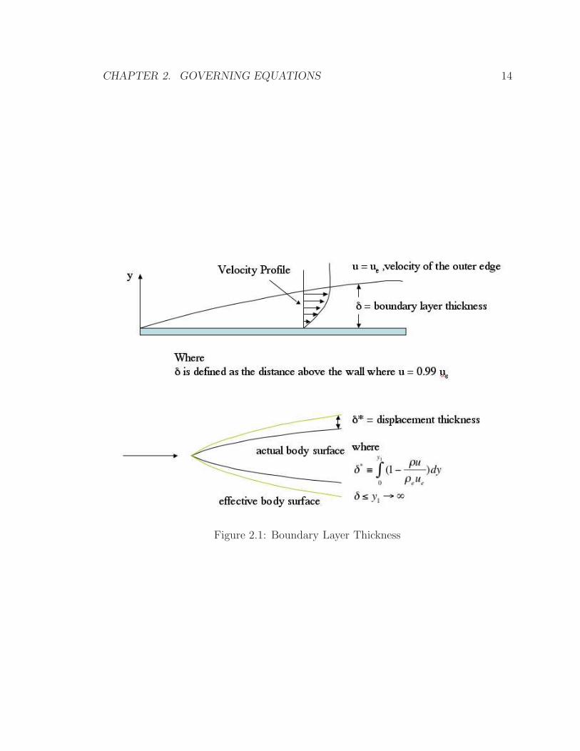
The Euler Equations are equivalent to an inviscid form of the Navier-Stokes equa-
tions. While the inviscid assumption might seem to limit their usefulness, in general,
the Euler Equations are widely applicable. This is because in viscous flow, nearly
all of the viscous behavior is concentrated in thin regions near surfaces (boundary
layers) where large velocity gradients exist. In flows where the boundary layer thick-
ness is negligible compared to the length scale of the body, inviscid flow can be safely
assumed around the effective body that is formed by the presence of boundary layers
on the surface of the original geometry, as illustrated in the figure 2.1.
For two-dimensional, steady flow while neglecting the normal stress in the y-
direction, τyy, the following equation is obtained,
ρu∂u
∂x+ ρv
∂v
∂y= −
∂p
∂y+
∂
∂x[µ(
∂u
∂x+∂u
∂y)].
In terms of non-dimensional variables,
ρ′u′∂u′
∂x′+ ρ′v′
∂v′
∂y′= −
1
γM2∞
∂p′
∂y′+
1
Re∞
∂
∂x′[µ′(
∂u′
∂x′+∂u′
∂y′)].
CHAPTER 2. GOVERNING EQUATIONS 14
Figure 2.1: Boundary Layer Thickness
CHAPTER 2. GOVERNING EQUATIONS 15
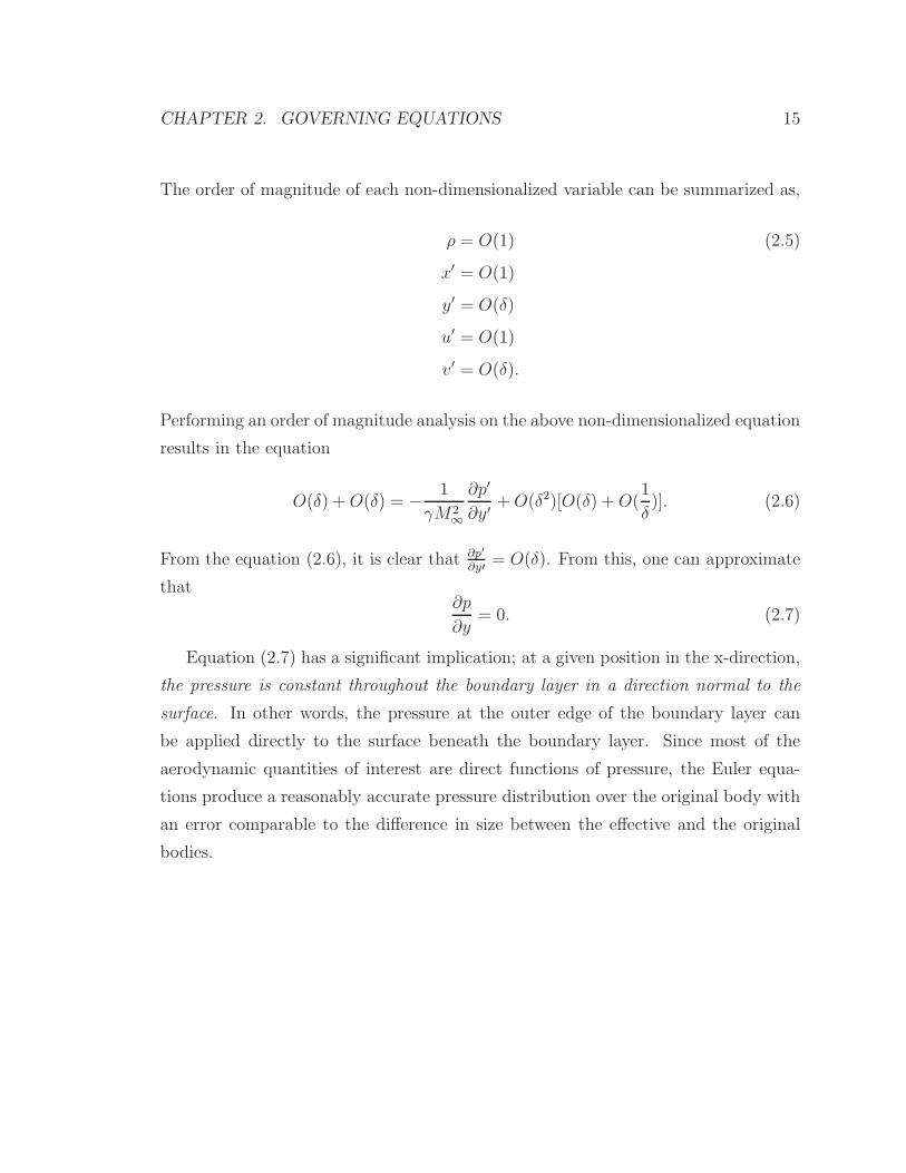
The order of magnitude of each non-dimensionalized variable can be summarized as,
ρ = O(1) (2.5)
x′ = O(1)
y′ = O(δ)
u′ = O(1)
v′ = O(δ).
Performing an order of magnitude analysis on the above non-dimensionalized equation
results in the equation
O(δ) +O(δ) = −1
γM2∞
∂p′
∂y′+O(δ2)[O(δ) +O(
1
δ)]. (2.6)
From the equation (2.6), it is clear that ∂p′
∂y′= O(δ). From this, one can approximate
that∂p
∂y= 0. (2.7)
Equation (2.7) has a significant implication; at a given position in the x-direction,
the pressure is constant throughout the boundary layer in a direction normal to the
surface. In other words, the pressure at the outer edge of the boundary layer can
be applied directly to the surface beneath the boundary layer. Since most of the
aerodynamic quantities of interest are direct functions of pressure, the Euler equa-
tions produce a reasonably accurate pressure distribution over the original body with
an error comparable to the difference in size between the effective and the original
bodies.
Chapter 3
Development of A Time-Spectral
Discrete Adjoint Solver
3.1 Benefits of Time-Spectral Discrete Adjoint
Method
The process of aerodynamic optimization, as discussed in the chapter 1, requires at
least two major components: an optimizer and a flow solver. The optimizer receives
objective function and constraint values from the flow solver at the given design iter-
ation and these values are fed into the optimizer in order to determine feasibility and
a descent direction for the set of parameters. Once a descent direction is found, a
proper step length is determined as well. In traditional gradient-based optimization,
these two components are sufficient for reaching a local optimum under a given opti-
mization problem statement. In this research, the concept of adjoints is employed as
the final component required to complete an adjoint gradient-based optimization. As
discussed and compared in sections 1.2 and 1.3, deriving gradient information from
adjoints reduces the number of flow solution evaluations by N − 1, where N is the
number of independent parameters in the objective function. The decrease reduces
the total number of runs from N + 1 to 2, regardless of the size of N .
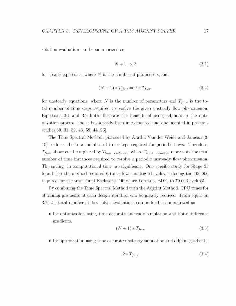
Applying the same logic, the effect of utilizing adjoint on the total number of flow
16
CHAPTER 3. DEVELOPMENT OF A TSM ADJOINT SOLVER 17
solution evaluation can be summarized as,
N + 1 ⇒ 2 (3.1)
for steady equations, where N is the number of parameters, and
(N + 1) ∗ Tflow ⇒ 2 ∗ Tflow (3.2)
for unsteady equations, where N is the number of parameters and Tflow is the to-
tal number of time steps required to resolve the given unsteady flow phenomenon.
Equations 3.1 and 3.2 both illustrate the benefits of using adjoints in the opti-
mization process, and it has already been implemented and documented in previous
studies[30, 31, 32, 43, 59, 44, 26].
The Time Spectral Method, pioneered by Arathi, Van der Weide and Jameson[3,
10], reduces the total number of time steps required for periodic flows. Therefore,
Tflow above can be replaced by Ttime−instances, where Ttime−instances represents the total
number of time instances required to resolve a periodic unsteady flow phenomenon.
The savings in computational time are significant. One specific study for Stage 35
found that the method required 6 times fewer multigrid cycles, reducing the 400,000
required for the traditional Backward Difference Formula, BDF, to 70,000 cycles[3].
By combining the Time Spectral Method with the Adjoint Method, CPU times for
obtaining gradients at each design iteration can be greatly reduced. From equation
3.2, the total number of flow solver evaluations can be further summarized as
• for optimization using time accurate unsteady simulation and finite difference
gradients,
(N + 1) ∗ Tflow (3.3)
• for optimization using time accurate unsteady simulation and adjoint gradients,
2 ∗ Tflow (3.4)
CHAPTER 3. DEVELOPMENT OF A TSM ADJOINT SOLVER 18
• optimization using the Time-Spectral Method for unsteady simulation and ad-
joint gradients,
2 ∗ TTS (3.5)
where TTS is defined as
TTS = RTS ∗ Tflow
and RTS designates the effectiveness of the Time Spectral Method for different appli-
cations. Finally, the effect of Time Spectral Adjoint Method is written as
(N + 1) ∗ Tflow ⇒ 2 ∗ Tflow ∗RTS = 2 ∗ TTS (3.6)
and the gain in CPU time is represented as
(N + 1) ∗ Tflow − 2 ∗ Tflow ∗RTS = Tflow ∗ (N + 1 − 2 ∗RTS). (3.7)
Development of the Time Spectral Adjoint Method is described in the following
three sections in more detail, including the governing equation for the Time-Spectral
Method, the implementation of the Discrete Adjoint Mehthod, and a description of
the optimization problem.
3.2 Flow Solver
3.2.1 Time Spectral Method
The Navier-Stokes equations in semi-discrete form can be written as
V∂w
∂t+R(w) = 0. (3.8)
When the flow follows a periodic pattern with known period T, the flow solution, w,
can be decomposed into a Fourier series, and as a result, V ∂w∂t
can be represented as
CHAPTER 3. DEVELOPMENT OF A TSM ADJOINT SOLVER 19
a function of w as follows,
wn =
N2−1∑
k=−N2
wkeiktn
Dtwn =
2π
T
N2−1∑
k=−N2
ikwkeiktn ,
where tn = n∆t. At this stage, Dtwn is a function of wk, so it must be converted into
a function of wk using an inverse transform,
wk =N−1∑
n=0
wne−ikn∆t.
Now, for the even number of N , Dtwn can be represented in terms of wn,
Dtwn =
2π
T
N2−1∑
m=−N2
+1
dmwn+m, (3.9)
where the coefficients[41] are given by
dm =
12(−1)m+1cot(πm
N) : m 6= 0
0 : m = 0.(3.10)
For the odd number of N ,
Dtwn =
2π
T
N−1
2∑
m= 1−N2
dmwn+m, (3.11)
and
dm =
12(−1)m+1cosec(πm
N) : m 6= 0
0 : m = 0.(3.12)
With both Dtwn and R(wn) as functions of wn, a new residual, R∗(wn), can be
CHAPTER 3. DEVELOPMENT OF A TSM ADJOINT SOLVER 20
defined:
R∗(wn) = V Dtwn +R(wn), (3.13)
Then, R∗(wn) is iteratively solved in pseudo-time until its convergence. The Time-
Spectral form of the governing equation is thus
V∂wn
∂τ+R∗(wn) = 0 (3.14)
where τ represents a pseudo time. The implementation of the time spectral adjoint
method requires an efficient solver for this equation.
3.2.2 URANS Flow Solver
A flow solver communicates with an optimizer in two ways: by returning objective
values – values of the cost function – as well as by returning constraint information,
as will be explained in section 3.4. Choosing a flow solver is no less important than
choosing an optimizer itself; most of the computational time involved in optimization
is spent evaluating the objective function and obtaining constraint information. Both
of the tasks are completed using flow solutions obtained by the solver[6, 8, 7, 9, 48].
Accuracy, CPU time, and memory storage space are important factors to consider
when choosing a flow solver. The solver selected for this work, SUmb, provides 2nd
order accuracy in space and 2nd order accuracy in time. It is an explicit solver, and
its required storage is approximately 100 bytes per node. CPU time depends mostly
on the computer architecture. However, due to its explicit, iterative nature, several
convergence techniques are implemented within SUmb[36, 41, 14, 15, 19, 18, 17, 21].
Faster convergence, low memory requirement, and reasonable accuracy makes it an
excellent choice for flows accompanying a shock.
SUmb
Due to its explicit nature, SUmb is better suited than an implicit solver for a large-
scale computation. This stems from a requirement that an implicit solver must store
information about the entire domain in a matrix which is subsequently inverted. An
CHAPTER 3. DEVELOPMENT OF A TSM ADJOINT SOLVER 21
explicit solver, on the other hand, needs only the bare minimum information required
to set up the problem and solve a solution.
One disadvantage of explicit solvers, however, is the prolonged time to conver-
gence. While the implicit solver was uses information from every cell in the domain,
the explicit solver knows of only those cells in its stencil at the time of each iteration.
Information must then travel through each stencil to reflect changes in the far right
cell from the far left cell and vice versa. This is one of the biggest penalties of the
explicit solver.
SUmb employs several techniques to overcome the slow convergence, namely:
• Runge-Kutta type Hybrid ODE solver
• Multiblock
• Parallelization.
Each of these will be further detailed in the following sections.
Hybrid ODE Solver Runge-Kutta ODE solvers are widely used because of their
simplicity of implementation and ability to handle large time-steps. The formulation
of the hybrid scheme is as follows:
w(0) = wn
w(1) = w(0) − αm∆tR(w0)
...
w(m+1) = w(0) − αm∆tR(w(m−1))
wn+1 = w(p).
(3.15)
CHAPTER 3. DEVELOPMENT OF A TSM ADJOINT SOLVER 22
The power of the hybrid scheme lies in the separate treatment of convective and
dissipative terms.
R(w(m)) = C(w(m)) +D(w(m))
D(w(m)) = βmD(w(m)) + (1 − βm)D(w(m−1)).
(3.16)
where C and D represent the convective and dissipative parts of the residual, respec-
tively. Separation of the convective and the dissipative part allows for the application
of different or optimized damping coefficients for different sets of governing equatios.
The convective term is dominant in the Euler equations, whereas in the Navier-Stokes
equations, the dissipative term is dominant. The separate adjustment of each term
produces an efficient amplification factor suitable for each set of equations. A five
stage scheme is widely used, and its coefficients are:
α1 =1
4, α2 =
1
6, α3 =
3
8, α4 =
1
2, α5 = 1,
β1 = 1, β2 = 0, β3 =14
25, β4 = 0, β5 =
11
25.
(3.17)
Multiblock Certain physical geometries are best represented by multiblock config-
urations. The inner boundary interface of a block becomes a set of halo cells which
need to be updated at every iteration to reflect changes in the flow variables. In an
explicit solver, this update process follows that of a single block configuration exactly,
except slight numerical errors due to the different paths for obtaining the same value.
In an implicit solver, however, the difference in the numbering system causes differ-
ent convergence behavior. This different numbering system is equivalent to having
different locations for off-diagonal terms.
Parallelization Parallelization is achieved by employing more than a single pro-
cessor to solve the discretized governing equation. Present-day computer technology
allows for machines containing large number of processors and to make the best use
CHAPTER 3. DEVELOPMENT OF A TSM ADJOINT SOLVER 23
of the available resources, multiple processors can execute code in parallel. Explicit
schemes are more suitable for parallelization than implicit schemes because with ev-
ery iteration each processor needs information from only those cells included in the
stencil. Parallelization should be built into the flow solver itself, because the logic of
the parallelized code is different from that of the sequential code.
For multi-CPU parallelization, the Message Passing Interface (MPI), is used. MPI
has long been the standard for parallel computing and has gained wide acceptance in
the CFD community. The MPICH programming library is very robust and available
for many different operating systems and compilers, including all major versions of
unix and linux, MAC OSX, and Microsoft Windows. In this study, MPICH for SGI
Origin 2000, SGI compiler, and Intel compiler has been used.
3.3 Discrete Adjoint Solver
Many realistic design problems involve a large number of parameters such that ob-
taining gradients by finite difference becomes prohibitively expensive. The adjoint
method, alternatively, can provide cheap gradient information reducing computa-
tional time roughly equivalent to evaluating a single flow solution. Therefore the total
computational cost for obtaining gradient information does not vary significantly for
a reasonably large number of design parameters.
3.3.1 Discrete vs. Continuous Adjoint
Adjoint solutions can be obtained through two different approaches: continuous ad-
joint and discrete adjoint formulations[43]. In the continuous adjoint approach, the
adjoint equation is first derived as a partial differential equation and then discretized.
In the discrete adjoint approach the discretized adjoint equation is derived directly
from the discretized cost function and flow equations. Hence, a discrete adjoint im-
plementation is inherently tied to the way in which the residual of the flow solver
is constructed. The continuous adjoint formulation has more freedom in the choice
of the complexity of discretization, while the discrete adjoint formulation has more
CHAPTER 3. DEVELOPMENT OF A TSM ADJOINT SOLVER 24
freedom in the choice of the cost function. In the limit of infinite grid resolution,
with sufficiently smooth geometries and smooth functions, both converge to the same
analytical solution as explored in detail in Nadarajah’s previous work[47],[43],[33].
In the continuous formulation, the adjoint solutions satisfy a set of governing
equations in the integral form, obtained after applying integration by parts. Thus, no
restriction is given to the discretization of the adjoint equations in the integral form
as long as the integral equations are satisfied. Because integration by parts involves
a conversion between a volume integral and a surface integral in the domain, only
cost functions that are a direct function of the flow variables on the surface can be
selected.
In the discrete formulation[4],[52], a discrete counterpart of integration by parts
is employed on the discretized governing equations. This has an implication in that
the order of discretization of the adjoint equations is directly tied to the order of
discretization of the flow solver. However, no restriction on the choice of the cost
function is required, as long as the adjoint variables satisfy the given set of equations.
The freedom to choose any cost function is the main reason for using the discrete
adjoint instead of the continuous adjoint in this research.
Implementation of the discrete adjoint requires obtaining exact jacobians for ev-
ery flow quantity in the discretized equations, which is not only very tedious but also
prone to human errors due to the complexity of certain quantities, such as the vis-
cosity coefficient, heat transfer coefficient and turbulent variables. Hand-derivations
of the flux jacobians proved a daunting task for some of the jacobians of the bound-
ary fluxes. In principle, automatic differentiation[54] can solve this problem since it
produces exact jacobians of any quantity by performing line-by-line differentiation
directly on the equations itself as long as its derivative is defined. However, even
though automatic differentiation reduces the possibilities of human errors consider-
ably, proper identification of inputs and outputs for each jacobian still needs careful
attention.
CHAPTER 3. DEVELOPMENT OF A TSM ADJOINT SOLVER 25
3.3.2 General Derivation of the Adjoint Equation
Let I represent a cost function of interest, such as drag or lift. In this case, I would
depend on the flow-field variables, w, and the geometry of the domain, F .
I = I(w,F).
The change of I[52] can be represented as
δI =∂IT
∂wδw +
∂IT
∂FδF, (3.18)
which depends on both δw and δF . The component of δI involving δw is much more
costly to calculate than δF of component. With this in mind, the concept of Lagrange
Multiplier, ψ, can be applied to the equation (3.18) so that the final form does not
contain any terms involving δw.
The residual can be defined as
R(w, F ) = 0,
which is also a function of w and F and its variable δR can be split into two parts
using the chain rule,
δR =
[
∂R
∂w
]
δw +
[
∂R
∂F
]
δF = 0. (3.19)
Noticing that δR is equivalent to zero, it can be freely added or subtracted to equation
3.18, which is represented as,
δI =∂IT
∂wδw +
∂IT
∂FδF − ψT
([
∂R
∂w
]
δw +
[
∂R
∂F
]
δF
)
=
∂IT
∂w− ψT
[
∂R
∂w
]
δw +
∂IT
∂F− ψT
[
∂R
∂F
]
δF.
CHAPTER 3. DEVELOPMENT OF A TSM ADJOINT SOLVER 26
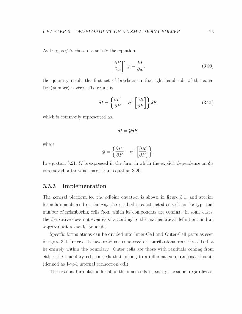
As long as ψ is chosen to satisfy the equation
[
∂R
∂w
]T
ψ =∂I
∂w, (3.20)
the quantity inside the first set of brackets on the right hand side of the equa-
tion(number) is zero. The result is
δI =
∂IT
∂F− ψT
[
∂R
∂F
]
δF, (3.21)
which is commonly represented as,
δI = GδF,
where
G =
∂IT
∂F− ψT
[
∂R
∂F
]
.
In equation 3.21, δI is expressed in the form in which the explicit dependence on δw
is removed, after ψ is chosen from equation 3.20.
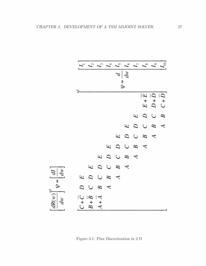
3.3.3 Implementation
The general platform for the adjoint equation is shown in figure 3.1, and specific
formulations depend on the way the residual is constructed as well as the type and
number of neighboring cells from which its components are coming. In some cases,
the derivative does not even exist according to the mathematical definition, and an
approximation should be made.
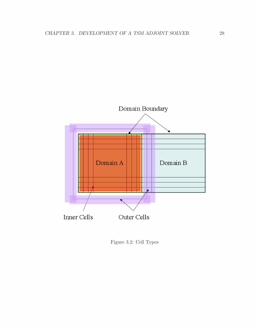
Specific formulations can be divided into Inner-Cell and Outer-Cell parts as seen
in figure 3.2. Inner cells have residuals composed of contributions from the cells that
lie entirely within the boundary. Outer cells are those with residuals coming from
either the boundary cells or cells that belong to a different computational domain
(defined as 1-to-1 internal connection cell).
The residual formulation for all of the inner cells is exactly the same, regardless of
CHAPTER 3. DEVELOPMENT OF A TSM ADJOINT SOLVER 27
Figure 3.1: Flux Discretization in 2 D
CHAPTER 3. DEVELOPMENT OF A TSM ADJOINT SOLVER 28
Figure 3.2: Cell Types
CHAPTER 3. DEVELOPMENT OF A TSM ADJOINT SOLVER 29
location, so the same derivative formulation can also be applied to all of the inner cells.
A description with further detail can be found in subsection 3.3.5 for inviscid flow and
3.3.6 for viscous flow. For the outer cells, residual formulations vary, depending on
the types of physical boundaries. The 1-to-1 internal connection cells follow the same
residual formulation as the inner cells, but have different indices as they are essentially
the same inner cells just separated by a different domain definition. Physical boundary
cells require much more attention and call for their own residual formulations.
While many physical boundary conditions exist, the following six conditions were
needed in this study, and their derivatives are developed in subsection 3.3.7:
• Farfield Boundary
• Euler Wall Boundary
• Viscous Wall Boundary
• Supersonic Inlet Boundary
• Supersonic Outlet Boundary
• Symmetric Boundary.
The biggest obstacle in developing the derivatives in equations 3.19 - 3.21 is de-
termining a reliable method of verification for the derived quantity. Three different
methods can be considered for evaluating the derivatives: Finite Difference, Complex
Derivative[38], and Direct Differentiation.
Finite differences are the simplest to implement, but a known drawback of the
method is cancellation error which can arise whenever a Jacobian matrix has near-
zero elements. Complex derivatives[39], on the other hand, produce accurate deriva-
tives, but their implementation is significantly more involved. The direct approach
was adopted in this work. The differentiation can be performed by hand or automat-
ically with dedicated software packages such as Tapenade. Automatic differentiation
involves treating a source code as a list of sequential functions (lines) which can be
differentiated in order following the chain rule. Both approaches were applied, be-
cause the results from Tapenade require the correct specification of a set of input
CHAPTER 3. DEVELOPMENT OF A TSM ADJOINT SOLVER 30
and output variables. When the result from the jacobian formulation matches that
of Tapenade as well as the result of line-by-line differentiation, the jacobian has been
verified.
Once the jacobian matrices and the objective function derivatives have been for-
mulated, the system is solved using PETSc, a matrix solver from Argonne National
Laboratory. While there may be a rather steep learning curve with PETSc, it has
proven to be a very effective software package. More information can be found in the
following website addresses:
• http://www.mcs.anl.gov/petsc/petsc-as/ for PETSc
• http://tapenade.inria.fr:8080/tapenade/index.jsp for Tapenade (automatic dif-
ferentiation program).
3.3.4 Derivatives of the Time-Spectral Terms
The derivatives of the time spectral term in equation 3.11,
Dtwn =
2π
T
N−1
2∑
m= 1−N2
dmwn+m,
play a crucial role in the successful implementation of the Time-Spectral Discrete
Adjoint Method. The time spectral term gathers contributions of the flow variables
over all the time instances, each of which is multiplied by the corresponding coefficient
in equation 3.12,
dm =
12(−1)m+1cosec(πm
N) : m 6= 0
0 : m = 0.
The sum is then added to the spatial residual as shown in equation 3.13,
R∗(wn) = V Dtwn +R(wn).
CHAPTER 3. DEVELOPMENT OF A TSM ADJOINT SOLVER 31
Following the definition of residual for the adjoint equations in equation 3.20,
[
∂R
∂w
]T
ψ =∂I
∂w,
the time spectral term needs to be differentiated at each time instance with respect
to each conservative flow variables at all the time instances. Thus, when the time
spectral term is differentiaed with respect to its own flow variables at different time
instances, the resulting jacobian becomes unity and only the coefficients survive.
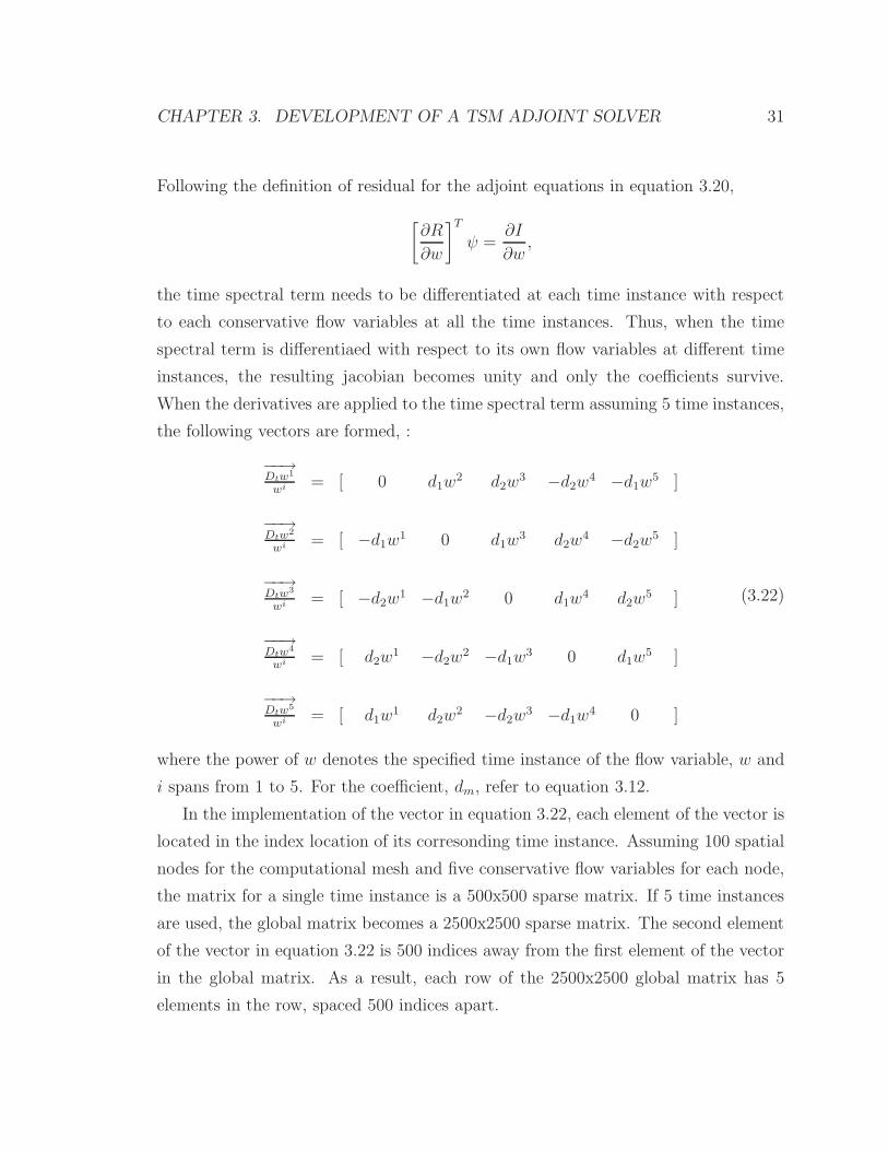
When the derivatives are applied to the time spectral term assuming 5 time instances,
the following vectors are formed, :
−−→Dtw
1
wi = [ 0 d1w2 d2w
3 −d2w4 −d1w
5 ]
−−→Dtw
2
wi = [ −d1w1 0 d1w
3 d2w4 −d2w
5 ]
−−→Dtw
3
wi = [ −d2w1 −d1w
2 0 d1w4 d2w
5 ]
−−→Dtw
4
wi = [ d2w1 −d2w
2 −d1w3 0 d1w
5 ]
−−→Dtw
5
wi = [ d1w1 d2w
2 −d2w3 −d1w
4 0 ]
(3.22)
where the power of w denotes the specified time instance of the flow variable, w and
i spans from 1 to 5. For the coefficient, dm, refer to equation 3.12.
In the implementation of the vector in equation 3.22, each element of the vector is
located in the index location of its corresonding time instance. Assuming 100 spatial
nodes for the computational mesh and five conservative flow variables for each node,
the matrix for a single time instance is a 500x500 sparse matrix. If 5 time instances
are used, the global matrix becomes a 2500x2500 sparse matrix. The second element
of the vector in equation 3.22 is 500 indices away from the first element of the vector
in the global matrix. As a result, each row of the 2500x2500 global matrix has 5
elements in the row, spaced 500 indices apart.
CHAPTER 3. DEVELOPMENT OF A TSM ADJOINT SOLVER 32
3.3.5 Inviscid Formulation
The Euler equations in differential form can be written as
∂w
∂t+∂f
∂x+∂g
∂y= 0. (3.23)
The equations put into integral form are[25]
∂
∂t
∫
S
wdS +
∫
∂S
[f(w)dy − g(w)dx] = 0 (3.24)
in two dimensions. In a full three-dimensional representation, surface vectors, Sx, Sy,
and Sz, replace dx and dy as follows,
ddt
∫
ΩWdV +
∫
∂Ω(FxdSx + FydSy + FzdSz) = 0
ddt
∫
ΩWdV +
∫
∂ΩΣi
−→Fi ·
−→dSi = 0,
(3.25)
wherep = (γ − 1)ρ(E − q2
2),
H = E + p
ρ= c2
γ−1+ q2
2.
(3.26)
The vector q is the flow velocity,
q2 = u2 + v2 + w2, c2 =γp
ρ, (3.27)
and c is the speed of sound. From the definitions of above, equation 3.25 is discretized,
and the fluxes are represented as
W =
ρ
ρu
ρv
ρw
ρE
, Fx =
ρu
ρuu+ p
ρuv
ρuw
ρuH
, Fy =
ρv
ρvu
ρvv + p
ρvw
ρvH
, Fz =
ρw
ρwu
ρwv
ρww + p
ρwH
.
(3.28)
CHAPTER 3. DEVELOPMENT OF A TSM ADJOINT SOLVER 33
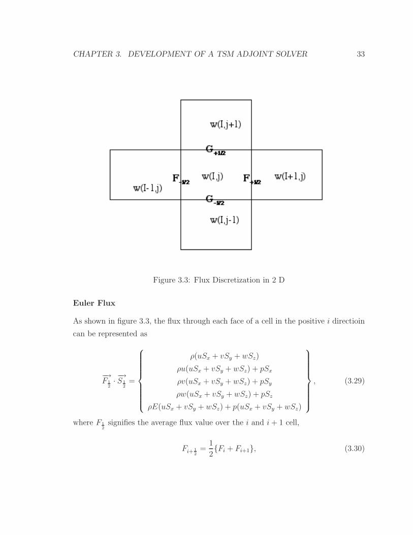
Figure 3.3: Flux Discretization in 2 D
Euler Flux
As shown in figure 3.3, the flux through each face of a cell in the positive i directioin
can be represented as
−→F 1
2
·−→S 1
2
=
ρ(uSx + vSy + wSz)
ρu(uSx + vSy + wSz) + pSx
ρv(uSx + vSy + wSz) + pSy
ρw(uSx + vSy + wSz) + pSz
ρE(uSx + vSy + wSz) + p(uSx + vSy + wSz)
, (3.29)
where F 1
2
signifies the average flux value over the i and i+ 1 cell,
Fi+ 1
2
=1
2Fi + Fi+1, (3.30)
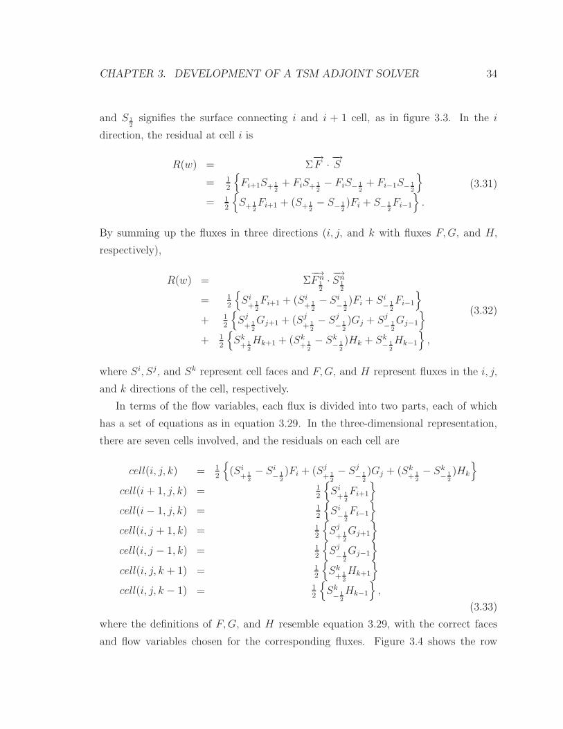
CHAPTER 3. DEVELOPMENT OF A TSM ADJOINT SOLVER 34
and S 1
2
signifies the surface connecting i and i + 1 cell, as in figure 3.3. In the i
direction, the residual at cell i is
R(w) = Σ−→F ·
−→S
= 12
Fi+1S+ 1
2
+ FiS+ 1
2
− FiS− 1
2
+ Fi−1S− 1
2
= 12
S+ 1
2
Fi+1 + (S+ 1
2
− S− 1
2
)Fi + S− 1
2
Fi−1
.
(3.31)
By summing up the fluxes in three directions (i, j, and k with fluxes F,G, and H,
respectively),
R(w) = Σ−→F n
1
2
·−→Sn
1
2
= 12
Si+ 1
2
Fi+1 + (Si+ 1
2
− Si− 1
2
)Fi + Si− 1
2
Fi−1
+ 12
Sj
+ 1
2
Gj+1 + (Sj
+ 1
2
− Sj
− 1
2
)Gj + Sj
− 1
2
Gj−1
+ 12
Sk+ 1
2
Hk+1 + (Sk+ 1
2
− Sk− 1
2
)Hk + Sk− 1
2
Hk−1
,
(3.32)
where Si, Sj, and Sk represent cell faces and F,G, and H represent fluxes in the i, j,
and k directions of the cell, respectively.
In terms of the flow variables, each flux is divided into two parts, each of which
has a set of equations as in equation 3.29. In the three-dimensional representation,
there are seven cells involved, and the residuals on each cell are
cell(i, j, k) = 12
(Si+ 1
2
− Si− 1
2
)Fi + (Sj
+ 1
2
− Sj
− 1
2
)Gj + (Sk+ 1
2
− Sk− 1
2
)Hk
cell(i+ 1, j, k) = 12
Si+ 1
2
Fi+1
cell(i− 1, j, k) = 12
Si− 1
2
Fi−1
cell(i, j + 1, k) = 12
Sj
+ 1
2
Gj+1
cell(i, j − 1, k) = 12
Sj
− 1
2
Gj−1
cell(i, j, k + 1) = 12
Sk+ 1
2
Hk+1
cell(i, j, k − 1) = 12
Sk− 1
2
Hk−1
,
(3.33)
where the definitions of F,G, and H resemble equation 3.29, with the correct faces
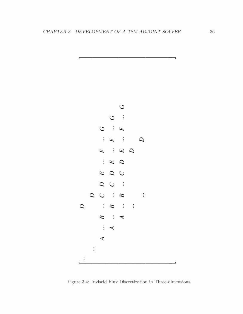
and flow variables chosen for the corresponding fluxes. Figure 3.4 shows the row
CHAPTER 3. DEVELOPMENT OF A TSM ADJOINT SOLVER 35
arrangement for the corresponding ∂R∂w
in matrix form.
Since the entire equation 3.32 constitutes a residual for one cell, in the derivative
of each cell with respect to the flow variables at every other cells, ∂R(w)∂w
, only those
cells involved in the residual calculation contributes to each row of the matrix. Hence,
each row of the matrix looks like those in figure 3.4, where
A = coefficient of the cell(i, j, k − 1)
B = coefficient of the cell(i, j − 1, k)
C = coefficient of the cell(i− 1, j, k)
D = coefficient of the cell(i, j, k)
E = coefficient of the cell(i+ 1, j, k)
F = coefficient of the cell(i, j + 1, k)
G = coefficient of the cell(i, j, k + 1)
as in equation 3.33.
For all of the inner cells whose contributing cells are within the computational
boundaries, the residual equation 3.32 is applied. However, the flux definition changes
for the cells beyond the boundaries. As a consequence, equation 3.29 needs modifi-
cations which make it suitable for the unique physical nature of each boundary. The
index of the contributing cell, as in equation 3.33 changes as well. Thus, the deriva-
tion presented in this section, equation 3.32, and equation 3.33 apply only to the
formulation of the inner cell flux. For special treatment of physical boundary cells,
refer to the 3.3.7
Artificial Dissipation
For inviscid equations, an implementation of artificial dissipation is mandatory, be-
cause it contributes heavily to the speed of convergence[25, 16] and is required for
the stability of the explicit, iterative methods used in SUmb. SUmb could be roughly
categorized as a central difference, explicit solver.
The flux balance in the residual can also be represented as
∂wj
∂t+ hj+ 1
2
+ hj− 1
2
= 0, (3.34)
CHAPTER 3. DEVELOPMENT OF A TSM ADJOINT SOLVER 36
Figure 3.4: Inviscid Flux Discretization in Three-dimensions
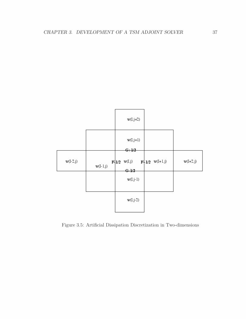
CHAPTER 3. DEVELOPMENT OF A TSM ADJOINT SOLVER 37
Figure 3.5: Artificial Dissipation Discretization in Two-dimensions
CHAPTER 3. DEVELOPMENT OF A TSM ADJOINT SOLVER 38
wherehj+ 1
2
= 12(fj+1 + fj) − dj 1
2
hj− 1
2
= 12(fj + fj−1) − dj− 1
2
dj+ 1
2
= ǫ2i+ 1
2
αi+ 1
2
(wi+1 − wi)
−ǫ4i+ 1
2
αi+ 1
2
(wi+2 − 3wi+1 + 3wi − wi−1)
dj+ 1
2
= ǫ2i− 1
2
αi− 1
2
(wi − wi−1)
−ǫ4i− 1
2
αi− 1
2
(wi+1 − 3wi + 3wi−1 − wi−2).
(3.35)
The expressionǫ2i+ 1
2
and ǫ4i+ 1
2
are adaptive coefficients, and αi+ 1
2
gives the proper scale
to the dissipative term. The expression ǫ is defined as follows,
νi,j =∣
∣
∣
pi+1,j−2pi,j+pi−1,j
pi+1,j+2pi,j+pi−1,j
∣
∣
∣
νi+ 1
2,j
= max(νi+2,j , νi+1,j , νi,j, νi−1,j)
ǫ2i+ 1
2,j
= min(12, k2ν
i+ 1
2,j)
ǫ4i+ 1
2,j
= min(0, k4 − ανi+ 1
2,j) ,
(3.36)
wherek2 = 1
k4 = 132
α = 2.
It should be noticed that, in equation 3.35, the artificial dissipation term spans across
four adjacent cells for each side of flux. With two artificial dissipation terms involved
in two-dimensional calculation, a five-cell stencil is involved in the flux balance equa-
tion for the given cell in one direction.
Another important fact is that the definitions of ν and ǫ involve absolute value
and min/max functions. By the definition of differentiation, a derivative of neither
of them exists. In the present development, this value is held constant.
CHAPTER 3. DEVELOPMENT OF A TSM ADJOINT SOLVER 39
The artificial dissipation balance term alone can be expressed as,
dj+ 1
2
− dj− 1
2
= −B+wj+2
+ (A+ + 3B+ −B−)wj+1
+ (−A+ − 3B+ − A− − 3B−)wj
+ (A− + 3B− −B+)wj+1
+ −B−wj−2,
(3.37)
whereA+ = ǫ2
j+ 1
2
αj+ 1
2
B+ = ǫ4j+ 1
2
αj+ 1
2
A− = ǫ2j− 1
2
αj− 1
2
B− = ǫ4j− 1
2
αj− 1
2
.
Figure 3.5 shows the five cell stencils involved in the calculation. In the full three-
dimensional representation, the complete artificial dissipation balance would appear
as,
CHAPTER 3. DEVELOPMENT OF A TSM ADJOINT SOLVER 40
di+ 1
2
− di− 1
2
+ dj+ 1
2
− dj− 1
2
+ dk+ 1
2
− dk− 1
2
= −Bi+wi+2,j,k
+ (Ai+ + 3Bi
+ −Bi−)wi+1,j,k
+ (−Ai+ − 3Bi
+ − Ai− − 3Bi
−)wi,j,k
+ (Ai− + 3Bi
− −Bi+)wi−1,j,k
+ −Bi−wi−2,j,k
+ −Bj+wi,j+2,k
+ (Aj+ + 3Bj
+ −Bj−)wi,j+1,k
+ (−Aj+ − 3Bj
+ − Aj− − 3Bj
−)wi,j,k
+ (Aj− + 3Bj
− −Bj+)wi,j−1,k
+ −Bj−wi,j−2,k
+ −Bk+wi,j,k+2
+ (Ak+ + 3Bk
+ −Bk−)wi,j,k+1
+ (−Ak+ − 3Bk
+ − Ak− − 3Bk
−)wi,j,k
+ (Ak− + 3Bk
− −Bk+)wi,j,k−1
+ −Bk−wi,j,k−2
+ −Bk−wi,j,k−2 ,
(3.38)
where the superscript i indicates i-direction and the subscript i indicates the cell
index.
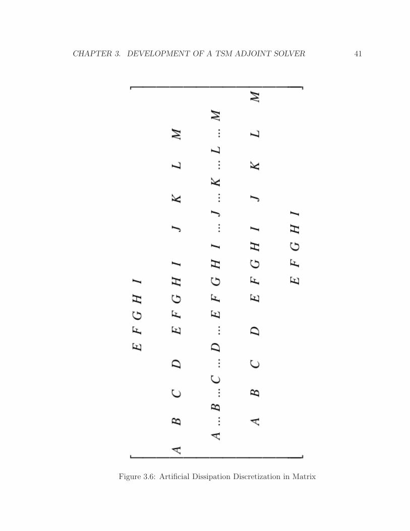
Figure 3.6 shows the matrix representation of the equation 3.38. Within the matrix,
each coefficient corresponds to a specific cell. The general relationships are
CHAPTER 3. DEVELOPMENT OF A TSM ADJOINT SOLVER 41
Figure 3.6: Artificial Dissipation Discretization in Matrix
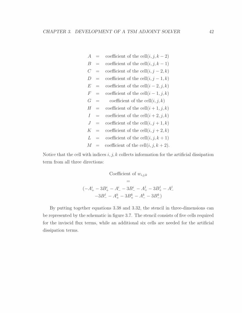
CHAPTER 3. DEVELOPMENT OF A TSM ADJOINT SOLVER 42
A = coefficient of the cell(i, j, k − 2)
B = coefficient of the cell(i, j, k − 1)
C = coefficient of the cell(i, j − 2, k)
D = coefficient of the cell(i, j − 1, k)
E = coefficient of the cell(i− 2, j, k)
F = coefficient of the cell(i− 1, j, k)
G = coefficient of the cell(i, j, k)
H = coefficient of the cell(i+ 1, j, k)
I = coefficient of the cell(i+ 2, j, k)
J = coefficient of the cell(i, j + 1, k)
K = coefficient of the cell(i, j + 2, k)
L = coefficient of the cell(i, j, k + 1)
M = coefficient of the cell(i, j, k + 2).
Notice that the cell with indices i, j, k collects information for the artificial dissipation
term from all three directions:
Coefficient of wi,j,k
=
(−Ai+ − 3Bi
+ − Ai− − 3Bi
− −Aj+ − 3Bj
+ − Aj−
−3Bj− − Ak
+ − 3Bk+ −Ak
− − 3Bk−)
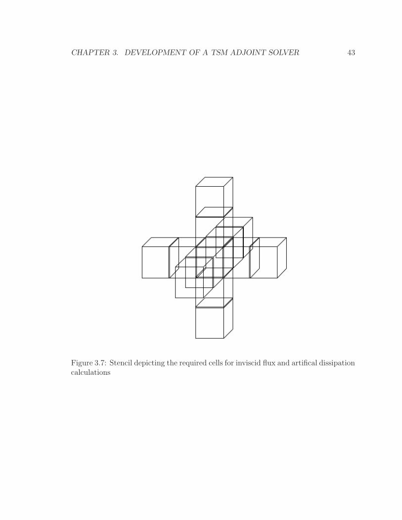
By putting together equations 3.38 and 3.32, the stencil in three-dimensions can
be represented by the schematic in figure 3.7. The stencil consists of five cells required
for the inviscid flux terms, while an additional six cells are needed for the artificial
dissipation terms.
CHAPTER 3. DEVELOPMENT OF A TSM ADJOINT SOLVER 43
Figure 3.7: Stencil depicting the required cells for inviscid flux and artifical dissipationcalculations
CHAPTER 3. DEVELOPMENT OF A TSM ADJOINT SOLVER 44
3.3.6 Viscous Formulation
Viscous Jacobian Calculation
The calculation of the viscous flux is based on the Divergence Theorem,
∫ ∫ ∫
V ol(−→ ·
−→F )dV =
∫ ∫
Surf
−→F · d−→a ,
where F represents flux vectors. In a discretized form, the right hand side of the
equation becomes∫ ∫
Surf
−→F · d−→a = ΣN
i=1(ΣMj=1FjSj)i,
where S,N, and M represent surfaces, the number of surfaces, and the number of
physical dimensions, respectively.
Terms for the viscous stress tensor from the Navier-Stokes equations(in one direc-
tion, u) can be written as
∫ ∫ ∫
V ol
∂(λ−→ ·
−→V + 2∂u
∂x)
∂x+µ∂(∂v
∂x+ ∂u
∂y)
∂y+µ∂(∂u
∂z+ ∂w
∂x)
∂zdV,
which can be written equivalently as
∫ ∫ ∫
V ol
−→ · (λ
−→ ·
−→V + 2
∂u
∂x, µ∂v
∂x+∂u
∂y, µ∂u
∂z+∂w
∂x)dV.
In this form, the Divergence Theorem can be directly applied to produce the following
result∫ ∫
Surf
(λ−→ ·
−→V + 2
∂u
∂x, µ∂v
∂x+∂u
∂y, µ∂u
∂z+∂w
∂x) · d−→n dS.
Each of the remaining viscous terms can be formulated in the same manner and are
listed here for completion;
∫ ∫
Surf
(λ−→ ·
−→V + 2
∂u
∂x, µ∂v
∂x+∂u
∂y, µ∂u
∂z+∂w
∂x) · d−→n dS
∫ ∫
Surf
(µ∂v
∂x+∂u
∂y, λ
−→ ·
−→V + 2
∂v
∂y, µ∂w
∂y+∂v
∂z) · d−→n dS
CHAPTER 3. DEVELOPMENT OF A TSM ADJOINT SOLVER 45
∫ ∫
Surf
(µ∂u
∂z+∂w
∂x, µ∂w
∂y+∂v
∂z, λ
−→ ·
−→V + 2
∂w
∂z) · d−→n dS
∫ ∫
Surf( uτxx + vτxy + wτxz + k ∂T
∂x,
uτyx + vτyy + wτyz + k ∂T∂y,
uτzx + wτzy + wτzz + k ∂T∂z
) · d−→n dS,
(3.39)
whereτxx = λ
−→ ·
−→V + 2∂u
∂x
τyy = λ−→ ·
−→V + 2∂v
∂y
τzz = λ−→ ·
−→V + 2∂w
∂z
τxy = µ ∂v∂x
+ ∂u∂y
τxz = µ∂u∂z
+ ∂w∂x
τyz = µ∂w∂y
+ ∂v∂z
τyx = τxy
τzx = τxz
τzy = τyz .
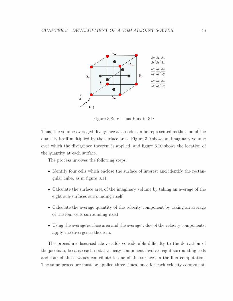
The formulation of the viscous term of the Navier-Stokes equations in equation
3.39 can be visually interpreted in figure 3.8. Red dots represent the nodal points
of the mesh, while black dots are the mid-surface points for each of the six surfaces
of the cube. Directional derivatives of each velocity component are obtained at the
nodal points, and their average values are obtained at each surface. In mathematical
terms, on each surface of the volume,
∂−→V i
∂−→x i
at the black dots = Σ1
4
∂−→V i
∂−→x i
over the four red dots, (3.40)
where the left hand side is the value computed at the black dot and the right hand
side consists of an average value over each of the red dots at the nodes of the surface.
Obtaining an Average Value at nodal points
In obtaining the nodal values, the same divergence theorem is applied to the velocity
vector itself rather than to the derivative of the velocity vector as in equation 3.39.
CHAPTER 3. DEVELOPMENT OF A TSM ADJOINT SOLVER 46
Figure 3.8: Viscous Flux in 3D
Thus, the volume-averaged divergence at a node can be represented as the sum of the
quantity itself multiplied by the surface area. Figure 3.9 shows an imaginary volume
over which the divergence theorem is applied, and figure 3.10 shows the location of
the quantity at each surface.
The process involves the following steps:
• Identify four cells which enclose the surface of interest and identify the rectan-
gular cube, as in figure 3.11
• Calculate the surface area of the imaginary volume by taking an average of the
eight sub-surfaces surrounding itself
• Calculate the average quantity of the velocity component by taking an average
of the four cells surrounding itself
• Using the average surface area and the average value of the velocity components,
apply the divergence theorem.
The procedure discussed above adds considerable difficulty to the derivation of
the jacobian, because each nodal velocity component involves eight surrounding cells
and four of those values contribute to one of the surfaces in the flux computation.
The same procedure must be applied three times, once for each velocity component.
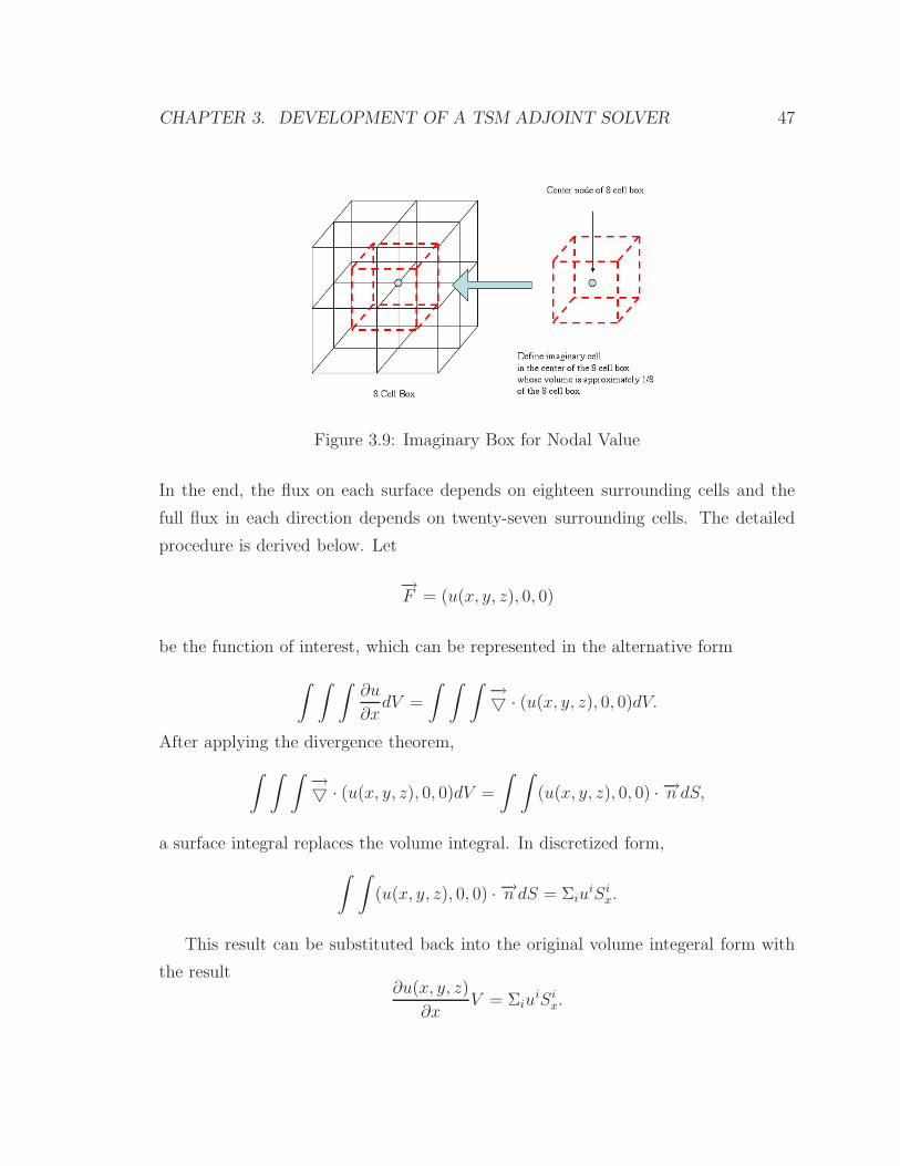
CHAPTER 3. DEVELOPMENT OF A TSM ADJOINT SOLVER 47
Figure 3.9: Imaginary Box for Nodal Value
In the end, the flux on each surface depends on eighteen surrounding cells and the
full flux in each direction depends on twenty-seven surrounding cells. The detailed
procedure is derived below. Let
−→F = (u(x, y, z), 0, 0)
be the function of interest, which can be represented in the alternative form
∫ ∫ ∫
∂u
∂xdV =
∫ ∫ ∫
−→ · (u(x, y, z), 0, 0)dV.
After applying the divergence theorem,
∫ ∫ ∫
−→ · (u(x, y, z), 0, 0)dV =
∫ ∫
(u(x, y, z), 0, 0) · −→n dS,
a surface integral replaces the volume integral. In discretized form,
∫ ∫
(u(x, y, z), 0, 0) · −→n dS = ΣiuiSi
x.
This result can be substituted back into the original volume integeral form with
the result∂u(x, y, z)
∂xV = Σiu
iSix.
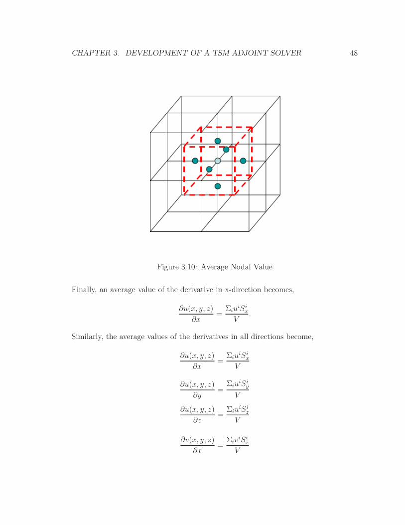
CHAPTER 3. DEVELOPMENT OF A TSM ADJOINT SOLVER 48
Figure 3.10: Average Nodal Value
Finally, an average value of the derivative in x-direction becomes,
∂u(x, y, z)
∂x=
ΣiuiSi
x
V.
Similarly, the average values of the derivatives in all directions become,
∂u(x, y, z)
∂x=
ΣiuiSi
x
V
∂u(x, y, z)
∂y=
ΣiuiSi
y
V
∂u(x, y, z)
∂z=
ΣiuiSi
z
V
∂v(x, y, z)
∂x=
ΣiviSi
x
V
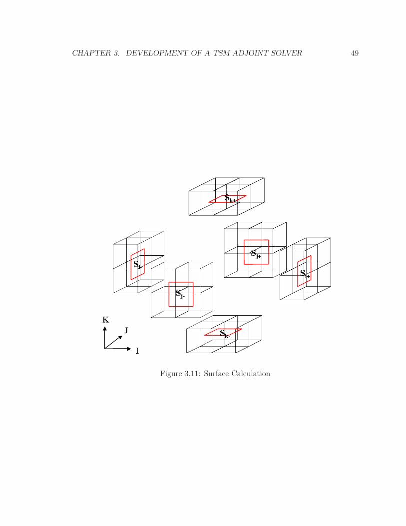
CHAPTER 3. DEVELOPMENT OF A TSM ADJOINT SOLVER 49
Figure 3.11: Surface Calculation
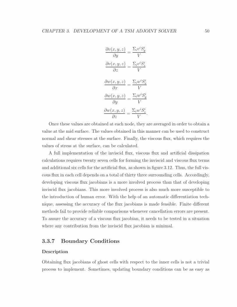
CHAPTER 3. DEVELOPMENT OF A TSM ADJOINT SOLVER 50
∂v(x, y, z)
∂y=
ΣiviSi
y
V
∂v(x, y, z)
∂z=
ΣiviSi
z
V
∂w(x, y, z)
∂x=
ΣiwiSi
x
V
∂w(x, y, z)
∂y=
ΣiwiSi
y
V
∂w(x, y, z)
∂z=
ΣiwiSi
z
V.
Once these values are obtained at each node, they are averaged in order to obtain a
value at the mid surface. The values obtained in this manner can be used to construct
normal and shear stresses at the surface. Finally, the viscous flux, which requires the
values of stress at the surface, can be calculated.
A full implementation of the inviscid flux, viscous flux and artificial dissipation
calculations requires twenty seven cells for forming the inviscid and viscous flux terms
and additional six cells for the artificial flux, as shown in figure 3.12. Thus, the full vis-
cous flux in each cell depends on a total of thirty three surrounding cells. Accordingly,
developing viscous flux jacobians is a more involved process than that of developing
inviscid flux jacobians. This more involved process is also much more susceptible to
the introduction of human error. With the help of an automatic differentiation tech-
nique, assessing the accuracy of the flux jacobians is made feasible. Finite different
methods fail to provide reliable comparisons whenever cancellation errors are present.
To assure the accuracy of a viscous flux jacobian, it needs to be tested in a situation
where any contribution from the inviscid flux jacobian is minimal.
3.3.7 Boundary Conditions
Description
Obtaining flux jacobians of ghost cells with respect to the inner cells is not a trivial
process to implement. Sometimes, updating boundary conditions can be as easy as
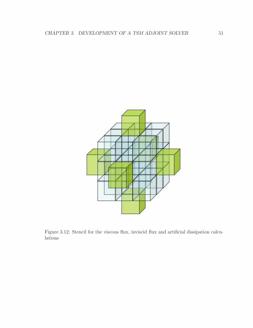
CHAPTER 3. DEVELOPMENT OF A TSM ADJOINT SOLVER 51
Figure 3.12: Stencil for the viscous flux, inviscid flux and artificial dissipation calcu-lations
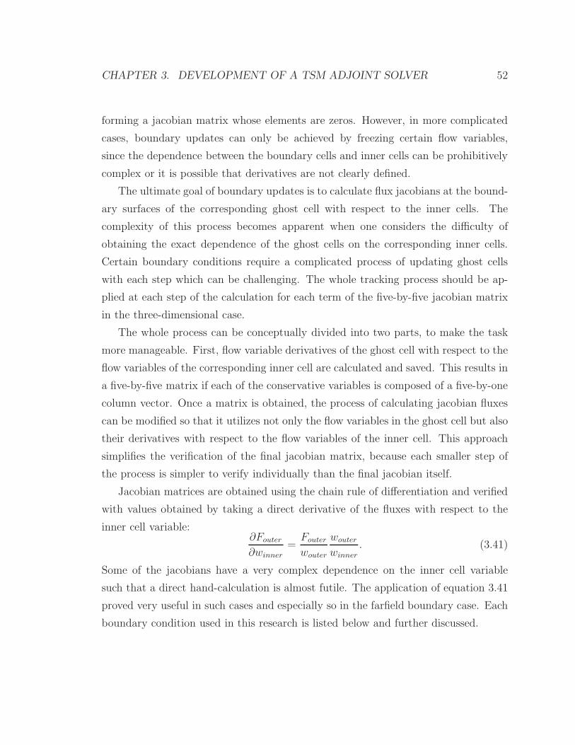
CHAPTER 3. DEVELOPMENT OF A TSM ADJOINT SOLVER 52
forming a jacobian matrix whose elements are zeros. However, in more complicated
cases, boundary updates can only be achieved by freezing certain flow variables,
since the dependence between the boundary cells and inner cells can be prohibitively
complex or it is possible that derivatives are not clearly defined.
The ultimate goal of boundary updates is to calculate flux jacobians at the bound-
ary surfaces of the corresponding ghost cell with respect to the inner cells. The
complexity of this process becomes apparent when one considers the difficulty of
obtaining the exact dependence of the ghost cells on the corresponding inner cells.
Certain boundary conditions require a complicated process of updating ghost cells
with each step which can be challenging. The whole tracking process should be ap-
plied at each step of the calculation for each term of the five-by-five jacobian matrix
in the three-dimensional case.
The whole process can be conceptually divided into two parts, to make the task
more manageable. First, flow variable derivatives of the ghost cell with respect to the
flow variables of the corresponding inner cell are calculated and saved. This results in
a five-by-five matrix if each of the conservative variables is composed of a five-by-one
column vector. Once a matrix is obtained, the process of calculating jacobian fluxes
can be modified so that it utilizes not only the flow variables in the ghost cell but also
their derivatives with respect to the flow variables of the inner cell. This approach
simplifies the verification of the final jacobian matrix, because each smaller step of
the process is simpler to verify individually than the final jacobian itself.
Jacobian matrices are obtained using the chain rule of differentiation and verified
with values obtained by taking a direct derivative of the fluxes with respect to the
inner cell variable:∂Fouter
∂winner
=Fouter
wouter
wouter
winner
. (3.41)
Some of the jacobians have a very complex dependence on the inner cell variable
such that a direct hand-calculation is almost futile. The application of equation 3.41
proved very useful in such cases and especially so in the farfield boundary case. Each
boundary condition used in this research is listed below and further discussed.
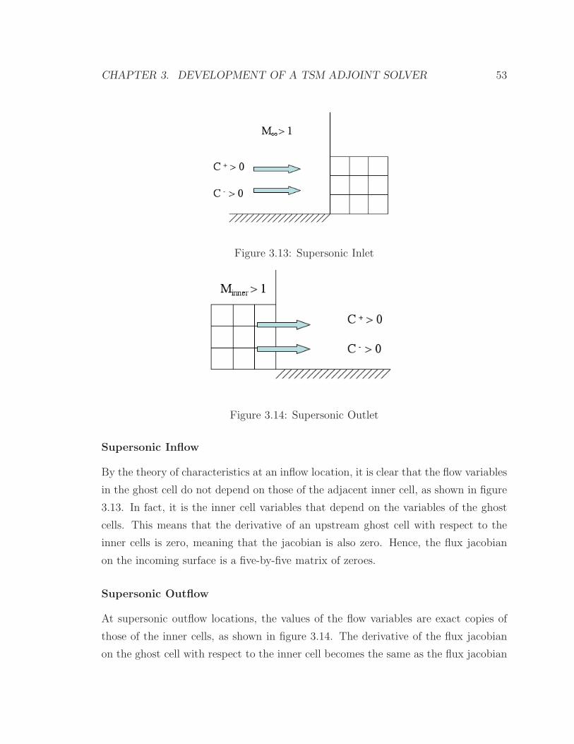
CHAPTER 3. DEVELOPMENT OF A TSM ADJOINT SOLVER 53
Figure 3.13: Supersonic Inlet
Figure 3.14: Supersonic Outlet
Supersonic Inflow
By the theory of characteristics at an inflow location, it is clear that the flow variables
in the ghost cell do not depend on those of the adjacent inner cell, as shown in figure
3.13. In fact, it is the inner cell variables that depend on the variables of the ghost
cells. This means that the derivative of an upstream ghost cell with respect to the
inner cells is zero, meaning that the jacobian is also zero. Hence, the flux jacobian
on the incoming surface is a five-by-five matrix of zeroes.
Supersonic Outflow
At supersonic outflow locations, the values of the flow variables are exact copies of
those of the inner cells, as shown in figure 3.14. The derivative of the flux jacobian
on the ghost cell with respect to the inner cell becomes the same as the flux jacobian
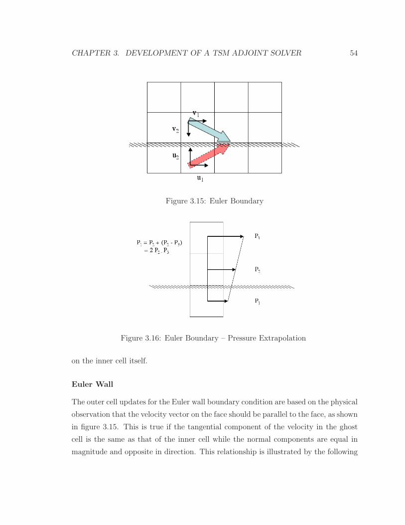
CHAPTER 3. DEVELOPMENT OF A TSM ADJOINT SOLVER 54
Figure 3.15: Euler Boundary
Figure 3.16: Euler Boundary – Pressure Extrapolation
on the inner cell itself.
Euler Wall
The outer cell updates for the Euler wall boundary condition are based on the physical
observation that the velocity vector on the face should be parallel to the face, as shown
in figure 3.15. This is true if the tangential component of the velocity in the ghost
cell is the same as that of the inner cell while the normal components are equal in
magnitude and opposite in direction. This relationship is illustrated by the following
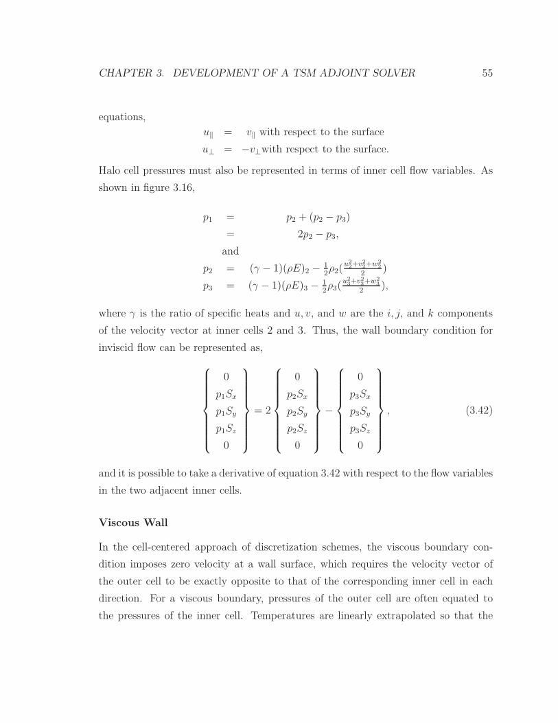
CHAPTER 3. DEVELOPMENT OF A TSM ADJOINT SOLVER 55
equations,
u‖ = v‖ with respect to the surface
u⊥ = −v⊥with respect to the surface.
Halo cell pressures must also be represented in terms of inner cell flow variables. As
shown in figure 3.16,
p1 = p2 + (p2 − p3)
= 2p2 − p3,
and
p2 = (γ − 1)(ρE)2 −12ρ2(
u22+v2
2+w22
2)
p3 = (γ − 1)(ρE)3 −12ρ3(
u23+v2
3+w2
3
2),
where γ is the ratio of specific heats and u, v, and w are the i, j, and k components
of the velocity vector at inner cells 2 and 3. Thus, the wall boundary condition for
inviscid flow can be represented as,
0
p1Sx
p1Sy
p1Sz
0
= 2
0
p2Sx
p2Sy
p2Sz
0
−
0
p3Sx
p3Sy
p3Sz
0
, (3.42)
and it is possible to take a derivative of equation 3.42 with respect to the flow variables
in the two adjacent inner cells.
Viscous Wall
In the cell-centered approach of discretization schemes, the viscous boundary con-
dition imposes zero velocity at a wall surface, which requires the velocity vector of
the outer cell to be exactly opposite to that of the corresponding inner cell in each
direction. For a viscous boundary, pressures of the outer cell are often equated to
the pressures of the inner cell. Temperatures are linearly extrapolated so that the
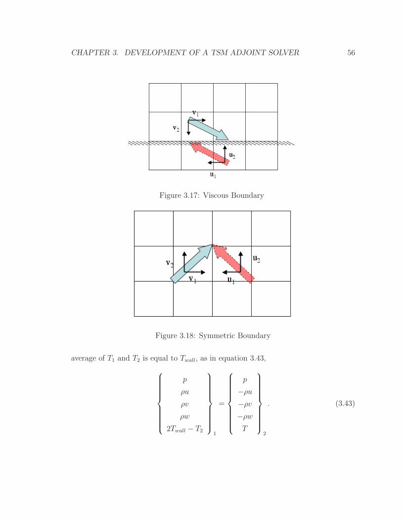
CHAPTER 3. DEVELOPMENT OF A TSM ADJOINT SOLVER 56
Figure 3.17: Viscous Boundary
Figure 3.18: Symmetric Boundary
average of T1 and T2 is equal to Twall, as in equation 3.43,
p
ρu
ρv
ρw
2Twall − T2
1
=
p
−ρu
−ρv
−ρw
T
2
. (3.43)
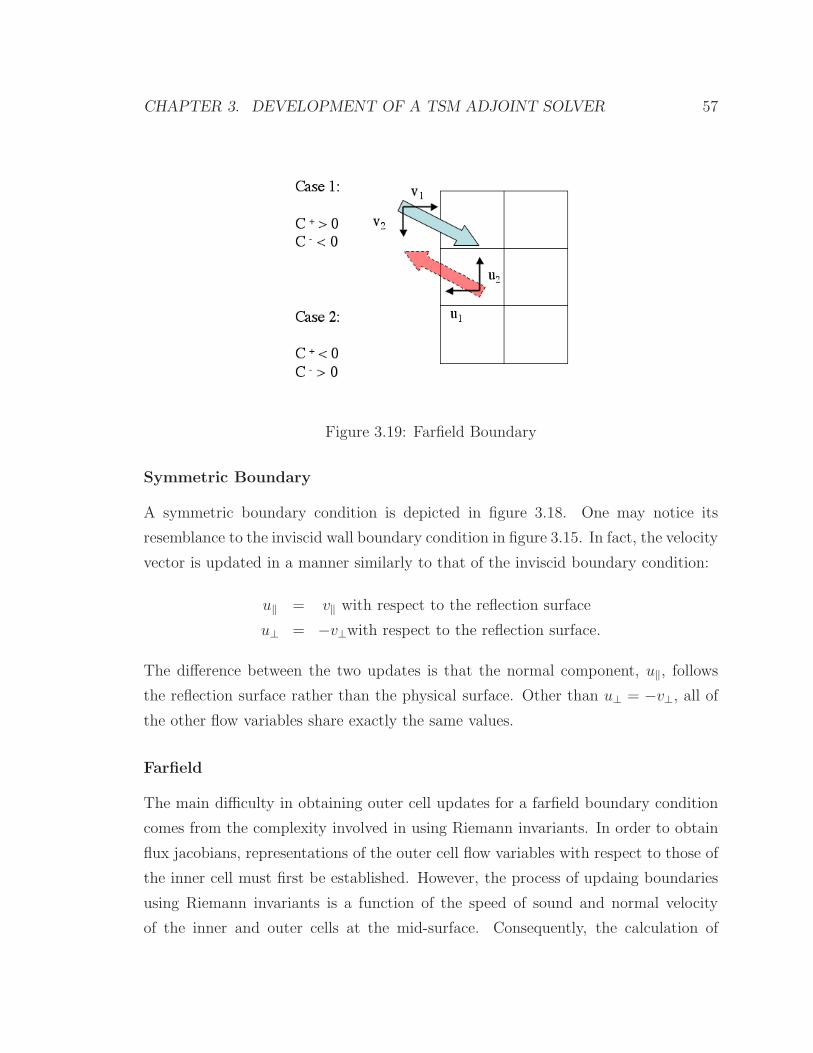
CHAPTER 3. DEVELOPMENT OF A TSM ADJOINT SOLVER 57
Figure 3.19: Farfield Boundary
Symmetric Boundary
A symmetric boundary condition is depicted in figure 3.18. One may notice its
resemblance to the inviscid wall boundary condition in figure 3.15. In fact, the velocity
vector is updated in a manner similarly to that of the inviscid boundary condition:
u‖ = v‖ with respect to the reflection surface
u⊥ = −v⊥with respect to the reflection surface.
The difference between the two updates is that the normal component, u‖, follows
the reflection surface rather than the physical surface. Other than u⊥ = −v⊥, all of
the other flow variables share exactly the same values.
Farfield
The main difficulty in obtaining outer cell updates for a farfield boundary condition
comes from the complexity involved in using Riemann invariants. In order to obtain
flux jacobians, representations of the outer cell flow variables with respect to those of
the inner cell must first be established. However, the process of updaing boundaries
using Riemann invariants is a function of the speed of sound and normal velocity
of the inner and outer cells at the mid-surface. Consequently, the calculation of
CHAPTER 3. DEVELOPMENT OF A TSM ADJOINT SOLVER 58
jacobians from Riemann invariants inherently requires performing derivatives on a set
of complex functions involving square root and power functions. The derivation and
implementation of the flux jacobian for a farfield boundary condition is an important
component of this research and is explained in detail throughout the rest of the
section.
Based on the theory of characteristics, extrapolated quantities can be categorized
as incoming and outgoing in a simple one dimensional analysis. Accordingly, Riemann
invariants are represented as,
R∞ = v∞ · −→n −2c∞γ − 1
Re = ve ·−→n +
2ceγ − 1
,
where e represents information coming from inner cells and ∞ represents extrapolated
information from the far field condition (outer cells). These two equations can be
manipulated to obtain
va · n⊥ =1
2(R∞ +Re)
ca =γ − 1
4(−R∞ +Re).
Further information on the tangential velocity is required in order to get the full
velocity vector. This information depends on the direction of the flow. For inflow, a
tangential velocity from the inner cell is used. For outflow, the tangential component
of the farfield velocity is used as follows,
va = ve · n‖ + va · n⊥ for outflow
va = v∞ · n‖ + va · n⊥ for inflow,(3.44)
where v∞ is an undisturbed free stream velocity and ve is that of the inner cell.
Now that we have a complete description of −→v and c, the speed of sound, only one
additional piece of information is required to close the system of equations. Entropy
CHAPTER 3. DEVELOPMENT OF A TSM ADJOINT SOLVER 59
can also be obtained by looking at the direction of the flow and as in equation 3.44,
sa = se for outflow
sa = s∞ for inflow.
In summary, one must obtain the following:
• ce and vn using the equations of Riemann invariants
• vt using the proper velocity vectors(based on the direction of the flow)
• S, entropy, based on the direction of the flow.
To apply this boundary condition to the Discrete Adjoint equation, one needs to
take derivatives of the farfield flux with respect to the flow variables of the inner cells.
A methodical application of the process can be summarized as follows:
• obtain the necessary flow variables using Riemann invariant extrapolation
• using the updated flow variables, obtain the flux jacobian at the farfield interface
• differentiate the flux with respect to the flow variables of the inner cell.
In order to minimize the probability of human error in complicated derivations, a
good practice for managing the complexity is the utilization of the chain rule of
differentiation. First, represent the flux derivative with respect to the generic flow
variables as a vector of partial derivative,
∂F
∂W= (
∂F
∂w1,∂F
∂w2,∂F
∂w3,∂F
∂w4,∂F
∂w5).
If the flux vector F is expanded into its five components, the derivatives of the flux
vector with respect to conservative variables can be represented in a more complete
form as∂F1
∂W= (
∂F1
∂w1,∂F1
∂w2,∂F1
∂w3,∂F1
∂w4,∂F1
∂w5)
∂F2
∂W= (
∂F2
∂w1,∂F2
∂w2,∂F2
∂w3,∂F2
∂w4,∂F2
∂w5)
CHAPTER 3. DEVELOPMENT OF A TSM ADJOINT SOLVER 60
∂F3
∂W= (
∂F3
∂w1
,∂F3
∂w2
,∂F3
∂w3
,∂F3
∂w4
,∂F3
∂w5
)
∂F4
∂W= (
∂F4
∂w1,∂F4
∂w2,∂F4
∂w3,∂F4
∂w4,∂F4
∂w5)
∂F5
∂W= (
∂F5
∂w1,∂F5
∂w2,∂F5
∂w3,∂F5
∂w4,∂F5
∂w5).
The above equation can then be represented in a more generic way by utilizing the
chain rule,
∂F1
∂W= (
∂F1
∂g1
∂g1
∂w1,∂F1
∂g1
∂g1
∂w2,∂F1
∂g1
∂g1
∂w3,∂F1
∂g1
∂g1
∂w4,∂F1
∂g1
∂g1
∂w5)
∂F2
∂W= (
∂F2
∂g2
∂g2
∂w1,∂F2
∂g2
∂g2
∂w2,∂F2
∂g2
∂g2
∂w3,∂F2
∂g2
∂g2
∂w4,∂F2
∂g2
∂g2
∂w5)
∂F3
∂W= (
∂F3
∂g3
∂g3
∂w1,∂F3
∂g3
∂g3
∂w2,∂F3
∂g3
∂g3
∂w3,∂F3
∂g3
∂g3
∂w4,∂F3
∂g3
∂g3
∂w5)
∂F4
∂W= (
∂F4
∂g4
∂g4
∂w1,∂F4
∂g4
∂g4
∂w2,∂F4
∂g4
∂g4
∂w3,∂F4
∂g4
∂g4
∂w4,∂F4
∂g4
∂g4
∂w5)
∂F5
∂W= (
∂F5
∂g5
∂g5
∂w1
,∂F5
∂g5
∂g5
∂w2
,∂F5
∂g5
∂g5
∂w3
,∂F5
∂g5
∂g5
∂w4
,∂F5
∂g5
∂g5
∂w5
)
where g is a set of intermediate functions that describe the complicated relation-
ship between F and W . This general relationship can be further broken down into
intermediate steps depending on the actual functions represented by g’s,
∂F
∂W=∂F
∂g1
∂g1
∂g2
∂g2
∂g3
∂g3
∂g4· · ·
∂gn
∂W
Derivation of Farfield Flux Jacobian
Using the chain rule, a full derivation of the farfield jacobian is here carried out with
the following definitions:
• the subscript B denotes values from a ghost cell
• the subscript JL denotes values from an internel cell
CHAPTER 3. DEVELOPMENT OF A TSM ADJOINT SOLVER 61
• the subscript S denotes values at the flux surface between the ghost and internal
cells.
With these definitions, the conservative variables at the ghost cell can be written as
functions of the variables in the internal cells:
ρB = f1( ~WJL)
PB = f2( ~WJL)
uB = f3( ~WJL)
vB = f4( ~WJL)
wB = f5( ~WJL),
where ~W is the vector of conservative variables. To determine the values at the flux
surface, a linear interpolation is used:
ρS =1
2(ρB + ρJL)
PS =1
2(PB + PJL)
uS =1
2(uB + uJL)
vS =1
2(vB + vJL)
wS =1
2(wB + wJL) .
From the values at the surface, a flux can be obtained using the following formulation,
G =
ρSVS
ρSVSuS + PSSx
ρSVSvS + PSSy
ρSVSwS + PSSz
ρSVSES + PSVS
,
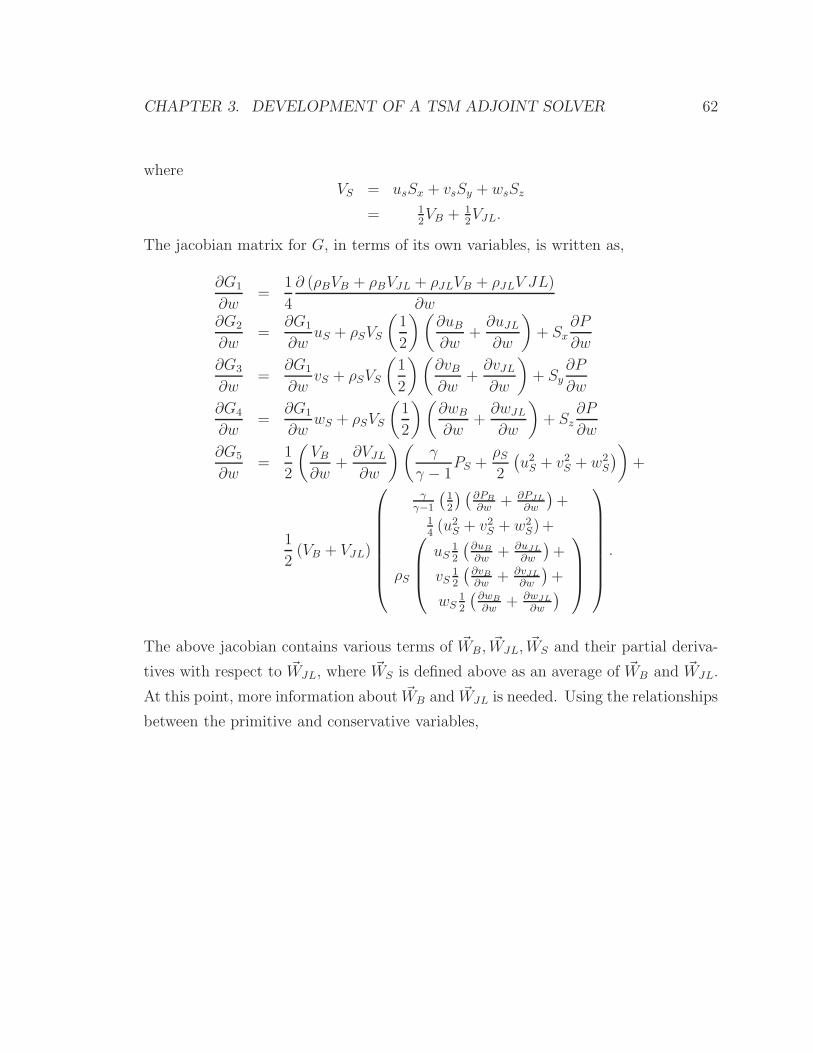
CHAPTER 3. DEVELOPMENT OF A TSM ADJOINT SOLVER 62
whereVS = usSx + vsSy + wsSz
= 12VB + 1
2VJL.
The jacobian matrix for G, in terms of its own variables, is written as,
∂G1
∂w=
1
4
∂ (ρBVB + ρBVJL + ρJLVB + ρJLV JL)
∂w∂G2
∂w=
∂G1
∂wuS + ρSVS
(
1
2
)(
∂uB
∂w+∂uJL
∂w
)
+ Sx
∂P
∂w
∂G3
∂w=
∂G1
∂wvS + ρSVS
(
1
2
)(
∂vB
∂w+∂vJL
∂w
)
+ Sy
∂P
∂w
∂G4
∂w=
∂G1
∂wwS + ρSVS
(
1
2
)(
∂wB
∂w+∂wJL
∂w
)
+ Sz
∂P
∂w
∂G5
∂w=
1
2
(
VB
∂w+∂VJL
∂w
)(
γ
γ − 1PS +
ρS
2
(
u2S + v2
S + w2S
)
)
+
1
2(VB + VJL)
γ
γ−1
(
12
) (
∂PB
∂w+ ∂PJL
∂w
)
+14(u2
S + v2S + w2
S)+
ρS
uS12
(
∂uB
∂w+ ∂uJL
∂w
)
+
vS12
(
∂vB
∂w+ ∂vJL
∂w
)
+
wS12
(
∂wB
∂w+ ∂wJL
∂w
)
.
The above jacobian contains various terms of ~WB, ~WJL, ~WS and their partial deriva-
tives with respect to ~WJL, where ~WS is defined above as an average of ~WB and ~WJL.
At this point, more information about ~WB and ~WJL is needed. Using the relationships
between the primitive and conservative variables,
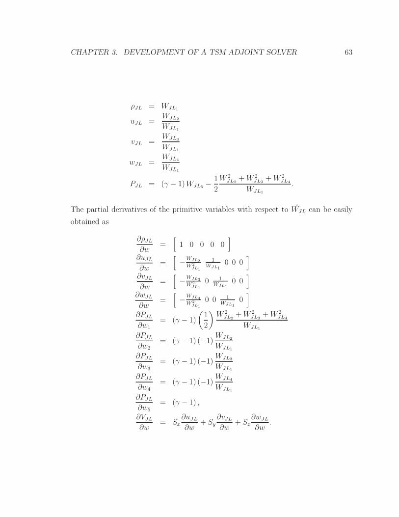
CHAPTER 3. DEVELOPMENT OF A TSM ADJOINT SOLVER 63
ρJL = WJL1
uJL =WJL2
WJL1
vJL =WJL3
WJL1
wJL =WJL4
WJL1
PJL = (γ − 1)WJL5−
1
2
W 2JL2
+W 2JL3
+W 2JL4
WJL1
.
The partial derivatives of the primitive variables with respect to ~WJL can be easily
obtained as
∂ρJL
∂w=
[
1 0 0 0 0]
∂uJL
∂w=
[
−WJL2
W 2JL1
1WJL1
0 0 0]
∂vJL
∂w=
[
−WJL3
W 2JL1
0 1WJL1
0 0]
∂wJL
∂w=
[
−WJL4
W 2JL1
0 0 1WJL1
0]
∂PJL
∂w1= (γ − 1)
(
1
2
)
W 2JL2
+W 2JL3
+W 2JL4
WJL1
∂PJL
∂w2= (γ − 1) (−1)
WJL2
WJL1
∂PJL
∂w3
= (γ − 1) (−1)WJL3
WJL1
∂PJL
∂w4= (γ − 1) (−1)
WJL4
WJL1
∂PJL
∂w5= (γ − 1) ,
∂VJL
∂w= Sx
∂uJL
∂w+ Sy
∂vJL
∂w+ Sz
∂wJL
∂w.
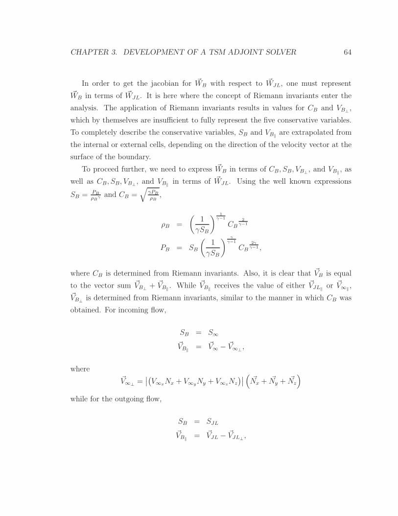
CHAPTER 3. DEVELOPMENT OF A TSM ADJOINT SOLVER 64
In order to get the jacobian for ~WB with respect to ~WJL, one must represent
~WB in terms of ~WJL. It is here where the concept of Riemann invariants enter the
analysis. The application of Riemann invariants results in values for CB and VB⊥,
which by themselves are insufficient to fully represent the five conservative variables.
To completely describe the conservative variables, SB and VB‖are extrapolated from
the internal or external cells, depending on the direction of the velocity vector at the
surface of the boundary.
To proceed further, we need to express ~WB in terms of CB, SB, VB⊥, and VB‖
, as
well as CB, SB, VB⊥, and VB‖
in terms of ~WJL. Using the well known expressions
SB = PB
ρBγ and CB =
√
γPB
ρB,
ρB =
(
1
γSB
) 1
γ−1
CB
2
γ−1
PB = SB
(
1
γSB
)γ
γ−1
CB
2γ
γ−1 ,
where CB is determined from Riemann invariants. Also, it is clear that ~VB is equal
to the vector sum ~VB⊥+ ~VB‖
. While ~VB‖receives the value of either ~VJL‖
or ~V∞‖,
~VB⊥is determined from Riemann invariants, similar to the manner in which CB was
obtained. For incoming flow,
SB = S∞
~VB‖= ~V∞ − ~V∞⊥
,
where
~V∞⊥=∣
∣
(
V∞xNx + V∞y
Ny + V∞zNz
)∣
∣
(
~Nx + ~Ny + ~Nz
)
while for the outgoing flow,
SB = SJL
~VB‖= ~VJL − ~VJL⊥
,
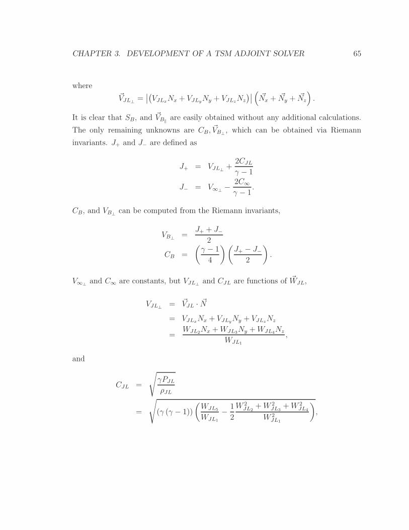
CHAPTER 3. DEVELOPMENT OF A TSM ADJOINT SOLVER 65
where
~VJL⊥=∣
∣
(
VJLxNx + VJLy
Ny + VJLzNz
)∣
∣
(
~Nx + ~Ny + ~Nz
)
.
It is clear that SB, and ~VB‖are easily obtained without any additional calculations.
The only remaining unknowns are CB, ~VB⊥, which can be obtained via Riemann
invariants. J+ and J− are defined as
J+ = VJL⊥+
2CJL
γ − 1
J− = V∞⊥−
2C∞
γ − 1.
CB, and VB⊥can be computed from the Riemann invariants,
VB⊥=
J+ + J−
2
CB =
(
γ − 1
4
)(
J+ − J−
2
)
.
V∞⊥and C∞ are constants, but VJL⊥
and CJL are functions of ~WJL,
VJL⊥= ~VJL · ~N
= VJLxNx + VJLy
Ny + VJLzNz
=WJL2
Nx +WJL3Ny +WJL4
Nz
WJL1
,
and
CJL =
√
γPJL
ρJL
=
√
(γ (γ − 1))
(
WJL5
WJL1
−1
2
W 2JL2
+W 2JL3
+W 2JL4
W 2JL1
)
,
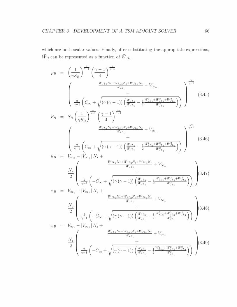
CHAPTER 3. DEVELOPMENT OF A TSM ADJOINT SOLVER 66
which are both scalar values. Finally, after substituting the appropriate expressions,
~WB can be represented as a function of ~WJL,
ρB =
(
1
γSB
)1
γ−1(
γ − 1
4
)2
γ−1
WJL2Nx+WJL3
Ny+WJL4Nz
WJL1
− V∞⊥
+
2γ−1
(
C∞ +
√
(γ (γ − 1))(
WJL5
WJL1
− 12
W 2JL2
+W 2JL3
+W 2JL4
W 2JL1
)
)
2
γ−1
(3.45)
PB = SB
(
1
γSB
)γ
γ−1(
γ − 1
4
)2γ
γ−1
WJL2Nx+WJL3
Ny+WJL4Nz
WJL1
− V∞⊥
+
2γ−1
(
C∞ +
√
(γ (γ − 1))(
WJL5
WJL1
− 12
W 2JL2
+W 2JL3
+W 2JL4
W 2JL1
)
)
2γ
γ−1
(3.46)
uB = V∞x− |V∞⊥
|Nx +
Nx
2
WJL2Nx+WJL3
Ny+WJL4Nz
WJL1
+ V∞⊥
+
2γ−1
(
−C∞ +
√
(γ (γ − 1))(
WJL5
WJL1
− 12
W 2JL2
+W 2JL3
+W 2JL4
W 2JL1
)
)
(3.47)
vB = V∞y− |V∞⊥
|Ny +
Ny
2
WJL2Nx+WJL3
Ny+WJL4Nz
WJL1
+ V∞⊥
+
2γ−1
(
−C∞ +
√
(γ (γ − 1))(
WJL5
WJL1
− 12
W 2JL2
+W 2JL3
+W 2JL4
W 2JL1
)
)
(3.48)
wB = V∞z− |V∞⊥
|Nz +
Nz
2
WJL2Nx+WJL3
Ny+WJL4Nz
WJL1
+ V∞⊥
+
2γ−1
(
−C∞ +
√
(γ (γ − 1))(
WJL5
WJL1
− 12
W 2JL2
+W 2JL3
+W 2JL4
W 2JL1
)
)
.(3.49)
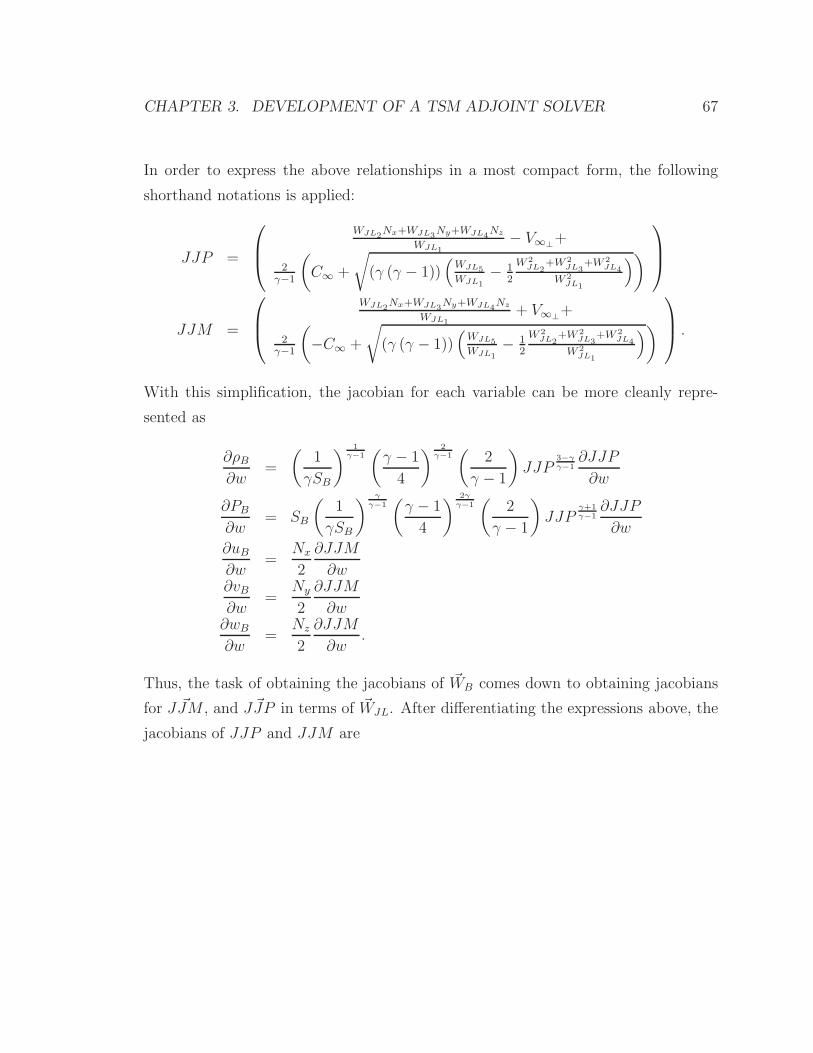
CHAPTER 3. DEVELOPMENT OF A TSM ADJOINT SOLVER 67
In order to express the above relationships in a most compact form, the following
shorthand notations is applied:
JJP =
WJL2Nx+WJL3
Ny+WJL4Nz
WJL1
− V∞⊥+
2γ−1
(
C∞ +
√
(γ (γ − 1))(
WJL5
WJL1
− 12
W 2JL2
+W 2JL3
+W 2JL4
W 2JL1
)
)
JJM =
WJL2Nx+WJL3
Ny+WJL4Nz
WJL1
+ V∞⊥+
2γ−1
(
−C∞ +
√
(γ (γ − 1))(
WJL5
WJL1
− 12
W 2JL2
+W 2JL3
+W 2JL4
W 2JL1
)
)
.
With this simplification, the jacobian for each variable can be more cleanly repre-
sented as
∂ρB
∂w=
(
1
γSB
)1
γ−1(
γ − 1
4
)2
γ−1(
2
γ − 1
)
JJP3−γγ−1
∂JJP
∂w
∂PB
∂w= SB
(
1
γSB
)γ
γ−1(
γ − 1
4
)2γ
γ−1(
2
γ − 1
)
JJPγ+1
γ−1∂JJP
∂w
∂uB
∂w=
Nx
2
∂JJM
∂w∂vB
∂w=
Ny
2
∂JJM
∂w∂wB
∂w=
Nz
2
∂JJM
∂w.
Thus, the task of obtaining the jacobians of ~WB comes down to obtaining jacobians
for ~JJM, and ~JJP in terms of ~WJL. After differentiating the expressions above, the
jacobians of JJP and JJM are
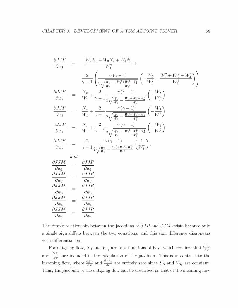
CHAPTER 3. DEVELOPMENT OF A TSM ADJOINT SOLVER 68
∂JJP
∂w1
= −W2Nx +W3Ny +W4Nz
W 21
+
2
γ − 1
γ (γ − 1)
2√
W5
W1−
W 22+W 2
3+W 2
4
W 21
(
−W5
W 21
+W 2
2 +W 23 +W 2
4
W 31
)
∂JJP
∂w2
=Nx
W1
+2
γ − 1
γ (γ − 1)
2√
W5
W1−
W 22+W 2
3+W 2
4
W 21
(
−W2
W 21
)
∂JJP
∂w3=
Ny
W1+
2
γ − 1
γ (γ − 1)
2√
W5
W1−
W 22+W 2
3+W 2
4
W 21
(
−W3
W 21
)
∂JJP
∂w4=
Nz
W1+
2
γ − 1
γ (γ − 1)
2√
W5
W1−
W 22+W 2
3+W 2
4
W 21
(
−W4
W 21
)
∂JJP
∂w2=
2
γ − 1
γ (γ − 1)
2√
W5
W1−
W 22+W 2
3+W 2
4
W 21
(
1
W 21
)
,
and∂JJM
∂w1=
∂JJP
∂w1
∂JJM
∂w2=
∂JJP
∂w2
∂JJM
∂w3=
∂JJP
∂w3
∂JJM
∂w4=
∂JJP
∂w4
∂JJM
∂w5=
∂JJP
∂w5.
The simple relationship between the jacobians of JJP and JJM exists because only
a single sign differs between the two equations, and this sign difference disappears
with differentiation.
For outgoing flow, SB and VB‖are now functions of ~WJL which requires that ∂SB
∂w
and∂VB‖
∂ware included in the calculation of the jacobian. This is in contrast to the
incoming flow, where ∂SB
∂wand
∂VB‖
∂ware entirely zero since SB and VB‖
are constant.
Thus, the jacobian of the outgoing flow can be described as that of the incoming flow
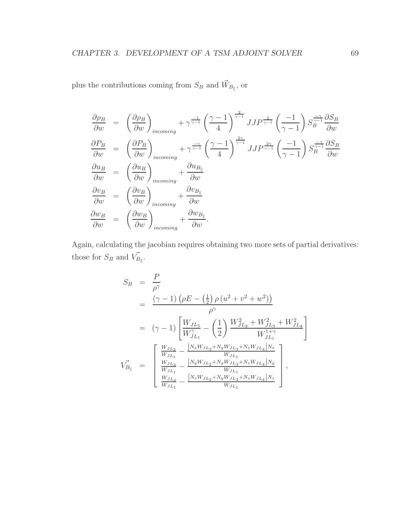
CHAPTER 3. DEVELOPMENT OF A TSM ADJOINT SOLVER 69
plus the contributions coming from SB and ~WB‖, or
∂ρB
∂w=
(
∂ρB
∂w
)
incoming
+ γ−1
γ−1
(
γ − 1
4
)2
γ−1
JJP2
γ−1
(
−1
γ − 1
)
S−γ
γ−1
B
∂SB
∂w
∂PB
∂w=
(
∂PB
∂w
)
incoming
+ γ−γ
γ−1
(
γ − 1
4
)2γ
γ−1
JJP2γ
γ−1
(
−1
γ − 1
)
S−γ
γ−1
B
∂SB
∂w
∂uB
∂w=
(
∂uB
∂w
)
incoming
+∂uB‖
∂w
∂vB
∂w=
(
∂vB
∂w
)
incoming
+∂vB‖
∂w
∂wB
∂w=
(
∂wB
∂w
)
incoming
+∂wB‖
∂w.
Again, calculating the jacobian requires obtaining two more sets of partial derivatives:
those for SB and ~VB‖.
SB =P
ργ
=(γ − 1)
(
ρE −(
12
)
ρ (u2 + v2 + w2))
ργ
= (γ − 1)
[
WJL5
WγJL1
−
(
1
2
)
W 2JL2
+W 2JL3
+W 2JL4
W1+γJL1
]
~VB‖=
WJL2
WJL1
−|NxWJL2
+NyWJL3+NzWJL4|Nx
WJL1
WJL3
WJL1
−|NyWJL2
+NyWJL3+NzWJL4|Ny
WJL1
WJL4
WJL1
−|NzWJL2
+NyWJL3+NzWJL4|Nz
WJL1
,
CHAPTER 3. DEVELOPMENT OF A TSM ADJOINT SOLVER 70
and their derivatives are given by,
∂uB‖
∂w=
[
−WJL2
W 2JL1
+(NxWJL2
+NyWJL3+NzWJL4)Nx
W 2JL1
1WJL1
− NxNx
WJL1
−NyNx
WJL1
−NzNx
WJL1
0
]
∂vB‖
∂w=
[
−WJL3
W 2JL1
+(NxWJL2
+NyWJL3+NzWJL4)Nx
W 2JL1
−NxNy
WJL1
1WJL1
− NyNy
WJL1
−NzNy
WJL1
0
]
∂wB‖
∂w=
[
−WJL4
W 2JL1
+(NxWJL2
+NyWJL3+NzWJL4)Nx
W 2JL1
−NxNz
WJL1
−NyNz
WJL1
1WJL1
− NzNz
WJL1
0
]
∂SB
∂w=
(γ − 1)
(
−γWJL5
Wγ+1
JL1
+ γ+12
W 2JL2
+W 2JL3
+W 2JL4
W2+γJL1
)
(γ − 1)
(
−WJL2
W1+γJL1
)
(γ − 1)
(
−WJL3
W1+γJL1
)
(γ − 1)
(
−WJL4
W1+γJL1
)
(γ − 1)(
1W
γJL1
)
T
.
3.3.8 Unsteady Boundary Conditions
The integral form of the Navier-Stokes equations can be formulated as
ddt
∫
VρdV +
∫
Sρ(−→u · −→n )dS = 0
ddt
∫
Vρ−→u dV +
∫
Sρ−→u (−→u · −→n )dS = −
∫
Spn⊥dS +
∫
S−→σ · −→n dS
ddt
∫
VρEdV +
∫
SρE(−→u · −→n )dS = −
∫
Sp−→u · −→n dS +
∫
S
−→u · −→σ · −→n dS
−∫
S−→q · −→n dS,
(3.50)
CHAPTER 3. DEVELOPMENT OF A TSM ADJOINT SOLVER 71
where
ρ = the density
p = the pressure−→u = the velocity vector−→σ = viscous stress tensor−→q = heat flux vector
E = total energy−→n = surface unit normal
V and S = volume and surface of the control volume, respectively
p = (γ − 1)ρ
E − 12(−→u · −→u )
.
For an unsteady flow, equation 3.50 requires the following specifications,
ρ(−→u · −→n ) => ρ(−→u −−→u surface ·−→n )
ρ−→u (−→u · −→n ) => ρ−→u (−→u −−→u surface ·−→n )
ρE(−→u · −→n ) => ρE(−→u −−→u surface ·−→n )
−∫
Sp−→u · −→n dS => −
∫
Sp−→u −−→u surface ·
−→n dS,
(3.51)
where −→u surface refers to the velocity of any moving surfaces.
In most cases with unsteady flow, a moving surface has a fixed velocity, such that
its derivative with respect to the flow variables becomes zero. However, the effect
of a moving surface is propagated into the flow field through multiplication with the
conservative flow variables, ρ, ρ−→u , and ρE. At a solid wall, (−→u · −→n ) becomes zero,
so contributions from the flux must also be. As explained in section 3.3.7, the only
meaningful contribution at a wall comes from p, as in the equation 3.42. The presence
of a wall velocity adds an additional term to equation 3.42,
∫
S
p(−→u surface)dS,
CHAPTER 3. DEVELOPMENT OF A TSM ADJOINT SOLVER 72
such that the equation becomes
Gwall =
0
pSx
pSy
pSy
p(−→u sruface ·−→S )
, (3.52)
where−→S is equal to (Sx, Sy, Sz), a surface vector in the x,y, and z directions.
In summary, the presence of a moving surface modifies the flux through that
surface. An effective velocity, −→u −−→u wall, must be applied to the flux contribution to
the inner cells to compensate. At the wall boundary, it also adds an additional term,
p(−→u surface ·−→S ), to the energy balance, as seen in equation 3.52.
3.3.9 Multiblock/Multiprocessor Implementation Issues
The quality of a computational mesh is a very important in determining the overall
quality of a CFD solution. However, different geometrics demand different meshing
schemes for generating a scientific mesh. In most cases, variations in the geometry
of interest make it extremely difficult to obtain high quality meshes using only one
meshing strategy for the entire geometry. In a multiblock approach, suitable meshing
schemes are chosen and applied to subsets of the total geometry. These individual
blocks are then grouped together, so the mesh quality of the entire geometry is as
good as that of each part. Thus, the implementation of a multiblock capability is an
important developement when dealing with realistic geometries.
The actual implementation of a multiblock, however, requires extra effort in book-
keeping boundary information as well as additional storage space. Within the flow
solver, the exchange of information between the blocks occurs through the updates
in the halo cells. The adjoint solver, however, requires an additional exchange of
index information for the halo cells, as shown in figure 3.20, 3.21, and figure 3.22. As
seen in figure 3.21, the contributions from donor cells must be properly accounted for
in the construction of each row of the matrix. This task is not necessarily straight
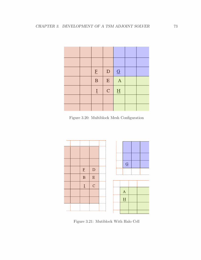
CHAPTER 3. DEVELOPMENT OF A TSM ADJOINT SOLVER 73
Figure 3.20: Multiblock Mesh Configuration
Figure 3.21: Mutiblock With Halo Cell
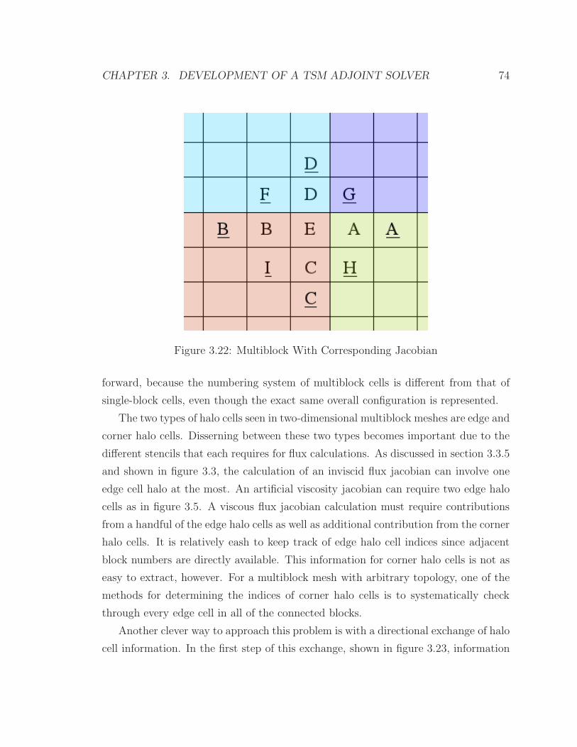
CHAPTER 3. DEVELOPMENT OF A TSM ADJOINT SOLVER 74
Figure 3.22: Multiblock With Corresponding Jacobian
forward, because the numbering system of multiblock cells is different from that of
single-block cells, even though the exact same overall configuration is represented.
The two types of halo cells seen in two-dimensional multiblock meshes are edge and
corner halo cells. Disserning between these two types becomes important due to the
different stencils that each requires for flux calculations. As discussed in section 3.3.5
and shown in figure 3.3, the calculation of an inviscid flux jacobian can involve one
edge cell halo at the most. An artificial viscosity jacobian can require two edge halo
cells as in figure 3.5. A viscous flux jacobian calculation must require contributions
from a handful of the edge halo cells as well as additional contribution from the corner
halo cells. It is relatively eash to keep track of edge halo cell indices since adjacent
block numbers are directly available. This information for corner halo cells is not as
easy to extract, however. For a multiblock mesh with arbitrary topology, one of the
methods for determining the indices of corner halo cells is to systematically check
through every edge cell in all of the connected blocks.
Another clever way to approach this problem is with a directional exchange of halo
cell information. In the first step of this exchange, shown in figure 3.23, information
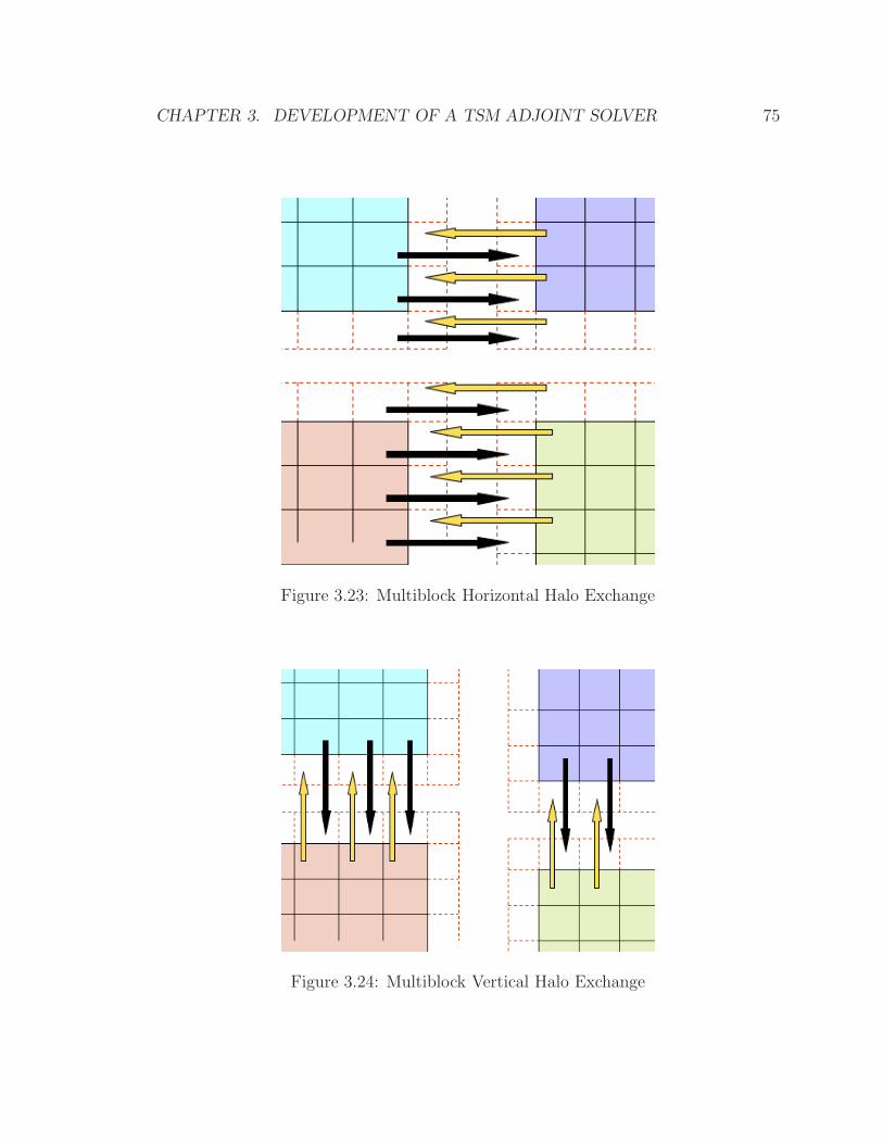
CHAPTER 3. DEVELOPMENT OF A TSM ADJOINT SOLVER 75
Figure 3.23: Multiblock Horizontal Halo Exchange
Figure 3.24: Multiblock Vertical Halo Exchange
CHAPTER 3. DEVELOPMENT OF A TSM ADJOINT SOLVER 76
is passed horizontally, although the corner cell information is not yet available. The
key idea of the directional update process is that the corner cell of any given block
is also an edge cell for a different block. Therefore, for a two-dimensional mesh,
once all of the edge cells have been updated in one direction, all of the required
corner cell information is available for exchange in the other direction, as shown in
figure 3.24. In three-dimensions, the corner cell information is available only after
completing exchanges in two of the three directions. The order of the updates can
be arbitrary, as long as all of the edges are updated in a given direction and all of
the directions are covered. Another thing to notice is the increase in the number of
off-diagonal elements due to the index shift in the multiblock representation. This
increased number of off-diagonal elements causes an increase in the convergence time.
The implementation of a multiprocessor capability was the final component de-
veloped for this research. The MPICH library, which follows the MPI standard,
is utilized. Adding multiprocessor capability also requires additional bookkeeping,
similar to these required for multiblock. The main difficulty in implementing this
capability is in interfacing with PETSc. PETSc, an external package, provides a
robust and scalable library, but learning its capabilities and limitations can require
large amounts of time and effort.
3.4 Optimization
3.4.1 Hick-Henne Bump Functions
In aerodynamic shape optimization using adjoint gradients, each grid point can be
used as a design variable. Perturbing each grid point, however, introduces disconti-
nuities. This difficulty can be overcome by applying a set of smooth functions that
perturb the initial geometry. In choosing such a function, the existence of continuous
and smooth derivatives is important. Abrupt changes in the derivative of the function,
although the function itself is continuous, could have adverse effects on any quantities
in the flow solver that require contributions from the gradient of the quantity. Once
a smooth curve is generated, it can be stretched or contracted locally to simulate a
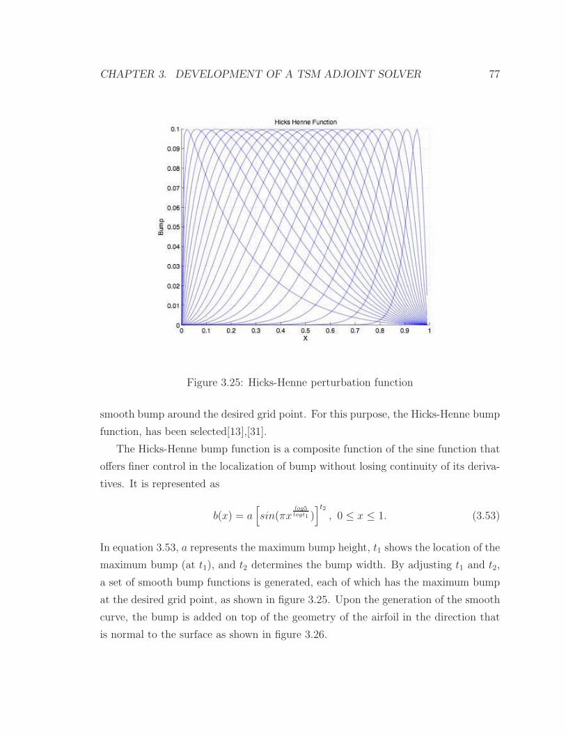
CHAPTER 3. DEVELOPMENT OF A TSM ADJOINT SOLVER 77
Figure 3.25: Hicks-Henne perturbation function
smooth bump around the desired grid point. For this purpose, the Hicks-Henne bump
function, has been selected[13],[31].
The Hicks-Henne bump function is a composite function of the sine function that
offers finer control in the localization of bump without losing continuity of its deriva-
tives. It is represented as
b(x) = a[
sin(πxlog5
logt1 )]t2
, 0 ≤ x ≤ 1. (3.53)
In equation 3.53, a represents the maximum bump height, t1 shows the location of the
maximum bump (at t1), and t2 determines the bump width. By adjusting t1 and t2,
a set of smooth bump functions is generated, each of which has the maximum bump
at the desired grid point, as shown in figure 3.25. Upon the generation of the smooth
curve, the bump is added on top of the geometry of the airfoil in the direction that
is normal to the surface as shown in figure 3.26.
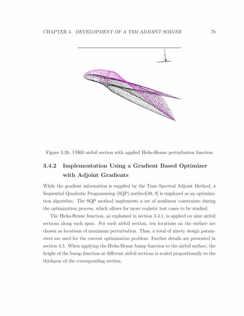
CHAPTER 3. DEVELOPMENT OF A TSM ADJOINT SOLVER 78
Figure 3.26: UH60 airfoil section with applied Hicks-Henne perturbation function
3.4.2 Implementation Using a Gradient Based Optimizer
with Adjoint Gradients
While the gradient information is supplied by the Time Spectral Adjoint Method, a
Sequential Quadratic Programming (SQP) method[48, 9] is employed as an optimiza-
tion algorithm. The SQP method implements a set of nonlinear constraints during
the optimization process, which allows for more realistic test cases to be studied.
The Hicks-Henne function, as explained in section 3.4.1, is applied on nine airfoil
sections along each span. For each airfoil section, ten locations on the surface are
chosen as locations of maximum perturbation. Thus, a total of ninety design param-
eters are used for the current optimization problem. Further details are presented in
section 4.5. When applying the Hicks-Henne bump function to the airfoil surface, the
height of the bump function at different airfoil sections is scaled proportionally to the
thickness of the corresponding section.
CHAPTER 3. DEVELOPMENT OF A TSM ADJOINT SOLVER 79
NPSOL
NPSOL[7] is a suite of software for solving constrained optimization problems and it
executes a dense SQP algorithm. The SQP method is especially effective for nonlin-
ear problems with objective and gradients which are expensive to evaluate. As its
name suggests, the SQP algorithm utilizes a quadratic representation of the objective
function and solves it sequentially.
Given a nonlinear optimization problem described by
minimize f(x)
subject to g(x) = 0,(3.54)
a new function, called a Lagrangian, can be found from the function and constraints
as
L(x, λ) = f(x) − λTg(x), (3.55)
where λ is a vector of Lagrange multipliers. This formulation converts a constrained
optimization problem into an unconstrained problem where the optimality conditions
(Karush-Kuhn-Tucker, KKT, Necessary conditions)[48] are given by
L(x, λ) = 0.
Value of x and λ are updated as
xk+1 = xk + pk
λk+1 = λk + νk
, (3.56)
where pk and νk are obtained by solving the linear equation,
2L(xk, λk)
pk
νk
= − L(xk, λk).
As a result, the original nonlinear objective function with nonlinear constraints,
CHAPTER 3. DEVELOPMENT OF A TSM ADJOINT SOLVER 80
equation 3.54, is recast as a new, quadratic objective function with linear constraints,
minimize over p 12pT [2
xxL(xk, λk)]p+ pT [xL(xk, λk)]
subject to [g(xk)]Tp+ g(xk) = 0,
(3.57)
where νk is the vector of Lagrange multipliers. Thus, the problem is transformed into
a minimization of a quadratic equation. In the Sequential Quadratic Programming
method, the above quadratic equation is solved at each iteration to find a new set of
points, (pk, νk), which are used to update (xk, λk), as shown in equation 3.56. Refer
to Appendix A for further details.
Chapter 4
Results
4.1 Description of the Test Cases
Upon completing the Time Spectral Adjoint Method implementation, it has been
validated using gradient information obtained from both an Automatic Differentiation
Method as well as a Finite Difference Method. Test cases were studied using three
different geometries: a NACA 0012 airfoil, a flat channel, and a UH60 helicopter
blade, as summarized in table 4.1. After verifying the gradient information obtained
from the Time Spectral Adjoint Method, a shape optimization was attempted on the
UH60 blade with a realistic set of constraints.
A NACA 0012 airfoil was used as the testbed geometry throughout the whole
development process due to its simple O-mesh topology. Once the adjoint gradient
information for the airfoil test case was validated against the jacobians generated
by automatic differentiation, the adjoint method was applied to the UH60 which
represents a realistic test case. Then, a shape optimization was attempted in order
to validate the new optimization methodology which relies on the adjoint gradients.
In practice, the UH60 test case was much more difficult to execute than that of the
NACA 0012 airfoil. A C-H mesh topology of the blade presented sub-facing problems
as well as bad quality meshes near both tips of the blade. To account for these issues,
multi-block and multi-processor capabilities were implemented in the early phase of
the research. Upon adding these capabilities, the complexity grew larger again, as
81
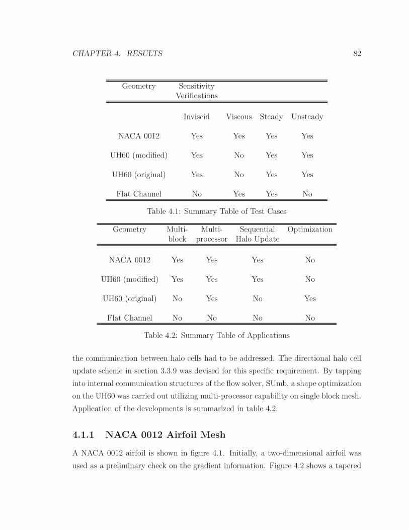
CHAPTER 4. RESULTS 82
Geometry SensitivityVerifications
Inviscid Viscous Steady Unsteady
NACA 0012 Yes Yes Yes Yes
UH60 (modified) Yes No Yes Yes
UH60 (original) Yes No Yes Yes
Flat Channel No Yes Yes No
Table 4.1: Summary Table of Test Cases
Geometry Multi- Multi- Sequential Optimizationblock processor Halo Update
NACA 0012 Yes Yes Yes No
UH60 (modified) Yes Yes Yes No
UH60 (original) No Yes No Yes
Flat Channel No No No No
Table 4.2: Summary Table of Applications
the communication between halo cells had to be addressed. The directional halo cell
update scheme in section 3.3.9 was devised for this specific requirement. By tapping
into internal communication structures of the flow solver, SUmb, a shape optimization
on the UH60 was carried out utilizing multi-processor capability on single block mesh.
Application of the developments is summarized in table 4.2.
4.1.1 NACA 0012 Airfoil Mesh
A NACA 0012 airfoil is shown in figure 4.1. Initially, a two-dimensional airfoil was
used as a preliminary check on the gradient information. Figure 4.2 shows a tapered
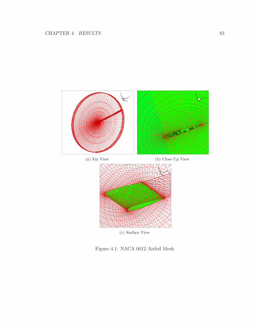
CHAPTER 4. RESULTS 83
X
Y
Z
(a) Far View
X
Y
Z
(b) Close Up View
X
Y
Z
(c) Surface View
Figure 4.1: NACA 0012 Airfoil Mesh
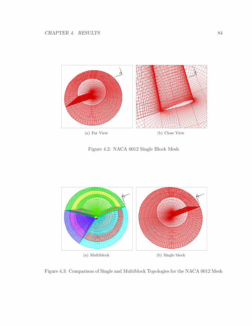
CHAPTER 4. RESULTS 84
Z
X
Y
(a) Far View
Z
X
Y
(b) Close View
Figure 4.2: NACA 0012 Single Block Mesh
X
Y
Z
(a) Multiblock
X
Y
Z
(b) Single block
Figure 4.3: Comparison of Single and Multiblock Topologies for the NACA 0012 Mesh
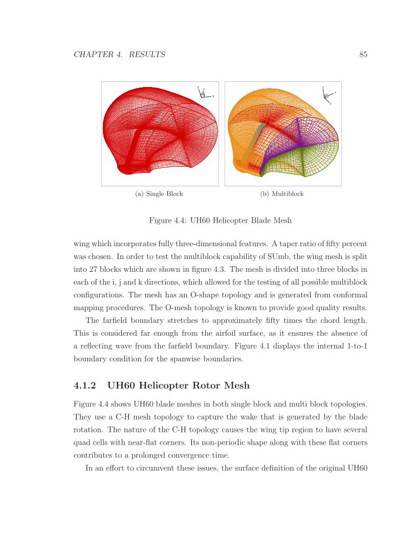
CHAPTER 4. RESULTS 85
Y
X
Z
(a) Single Block
X
Y
Z
(b) Multiblock
Figure 4.4: UH60 Helicopter Blade Mesh
wing which incorporates fully three-dimensional features. A taper ratio of fifty percent
was chosen. In order to test the multiblock capability of SUmb, the wing mesh is split
into 27 blocks which are shown in figure 4.3. The mesh is divided into three blocks in
each of the i, j and k directions, which allowed for the testing of all possible multiblock
configurations. The mesh has an O-shape topology and is generated from conformal
mapping procedures. The O-mesh topology is known to provide good quality results.
The farfield boundary stretches to approximately fifty times the chord length.
This is considered far enough from the airfoil surface, as it ensures the absence of
a reflecting wave from the farfield boundary. Figure 4.1 displays the internal 1-to-1
boundary condition for the spanwise boundaries.
4.1.2 UH60 Helicopter Rotor Mesh
Figure 4.4 shows UH60 blade meshes in both single block and multi block topologies.
They use a C-H mesh topology to capture the wake that is generated by the blade
rotation. The nature of the C-H topology causes the wing tip region to have several
quad cells with near-flat corners. Its non-periodic shape along with these flat corners
contributes to a prolonged convergence time.
In an effort to circumvent these issues, the surface definition of the original UH60
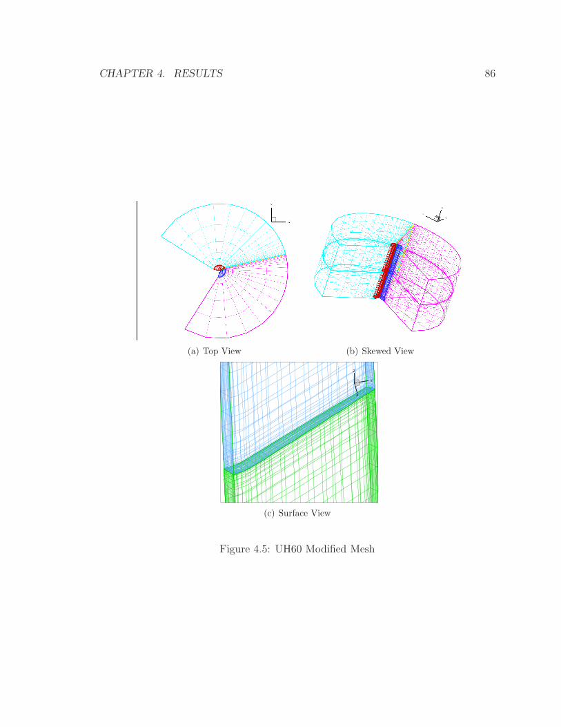
CHAPTER 4. RESULTS 86
(a) Top View (b) Skewed View
X
Y
Z
(c) Surface View
Figure 4.5: UH60 Modified Mesh
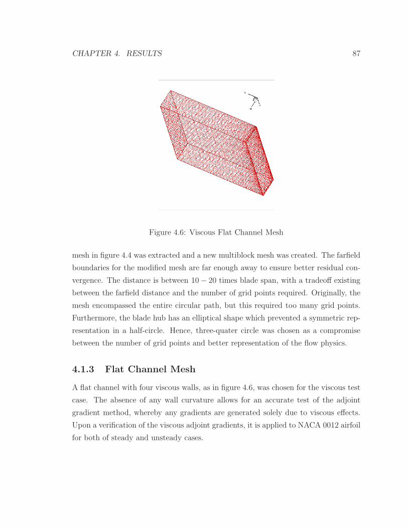
CHAPTER 4. RESULTS 87
Figure 4.6: Viscous Flat Channel Mesh
mesh in figure 4.4 was extracted and a new multiblock mesh was created. The farfield
boundaries for the modified mesh are far enough away to ensure better residual con-
vergence. The distance is between 10− 20 times blade span, with a tradeoff existing
between the farfield distance and the number of grid points required. Originally, the
mesh encompassed the entire circular path, but this required too many grid points.
Furthermore, the blade hub has an elliptical shape which prevented a symmetric rep-
resentation in a half-circle. Hence, three-quater circle was chosen as a compromise
between the number of grid points and better representation of the flow physics.
4.1.3 Flat Channel Mesh
A flat channel with four viscous walls, as in figure 4.6, was chosen for the viscous test
case. The absence of any wall curvature allows for an accurate test of the adjoint
gradient method, whereby any gradients are generated solely due to viscous effects.
Upon a verification of the viscous adjoint gradients, it is applied to NACA 0012 airfoil
for both of steady and unsteady cases.
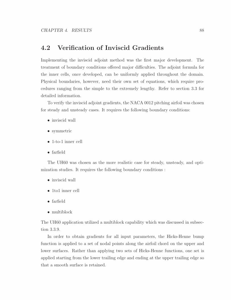
CHAPTER 4. RESULTS 88
4.2 Verification of Inviscid Gradients
Implementing the inviscid adjoint method was the first major development. The
treatment of boundary conditions offered major difficulties. The adjoint formula for
the inner cells, once developed, can be uniformly applied throughout the domain.
Physical boundaries, however, need their own set of equations, which require pro-
cedures ranging from the simple to the extremely lengthy. Refer to section 3.3 for
detailed information.
To verify the inviscid adjoint gradients, the NACA 0012 pitching airfoil was chosen
for steady and unsteady cases. It requires the following boundary conditions:
• inviscid wall
• symmetric
• 1-to-1 inner cell
• farfield
The UH60 was chosen as the more realistic case for steady, unsteady, and opti-
mization studies. It requires the following boundary conditions :
• inviscid wall
• 1to1 inner cell
• farfield
• multiblock
The UH60 application utilized a multiblock capability which was discussed in subsec-
tion 3.3.9.
In order to obtain gradients for all input parameters, the Hicks-Henne bump
function is applied to a set of nodal points along the airfoil chord on the upper and
lower surfaces. Rather than applying two sets of Hicks-Henne functions, one set is
applied starting from the lower trailing edge and ending at the upper trailing edge so
that a smooth surface is retained.
CHAPTER 4. RESULTS 89
Figure 4.7: Inviscid, Steady Gradient Comparison for the NACA 0012
4.2.1 Steady Gradient Comparison
Figure 4.7 shows a comparison between the adjoint and finite difference gradients of
a drag coefficient for NACA 0012 airfoil. A transonic case with a mach number of
0.8 was simulated and produced a very good match. The Hicks-Henne function was
applied to the lower and upper surface.
4.2.2 Unsteady
Figure 4.8-4.10 shows an application of the Time Spectral Adjoint method to the
NACA 0012 for the same transonic conditions. The gradient shown is that of a
summation of cost function, a drag coefficient, over all time instances. Again, a very
good match is obtained between the adjoint and finite difference gradients. In figure
4.8 - 4.10, gradient comparisons are shown for varying angular frequencies, from 5 to
140. In figure 4.11, the three subfigures, 4.8 - 4.10, are plotted together to visualize
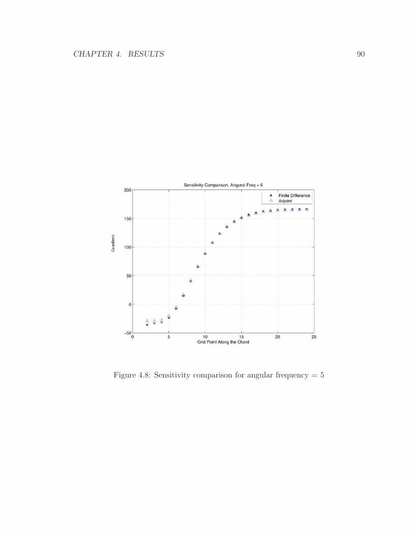
CHAPTER 4. RESULTS 90
Figure 4.8: Sensitivity comparison for angular frequency = 5
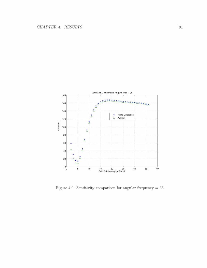
CHAPTER 4. RESULTS 91
Figure 4.9: Sensitivity comparison for angular frequency = 35

CHAPTER 4. RESULTS 92
Figure 4.10: Sensitivity comparison for angular frequency = 140
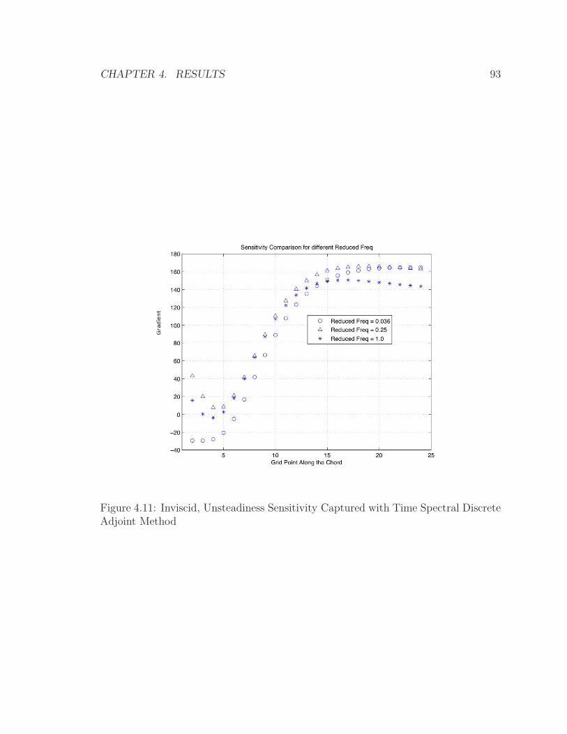
CHAPTER 4. RESULTS 93
Figure 4.11: Inviscid, Unsteadiness Sensitivity Captured with Time Spectral DiscreteAdjoint Method
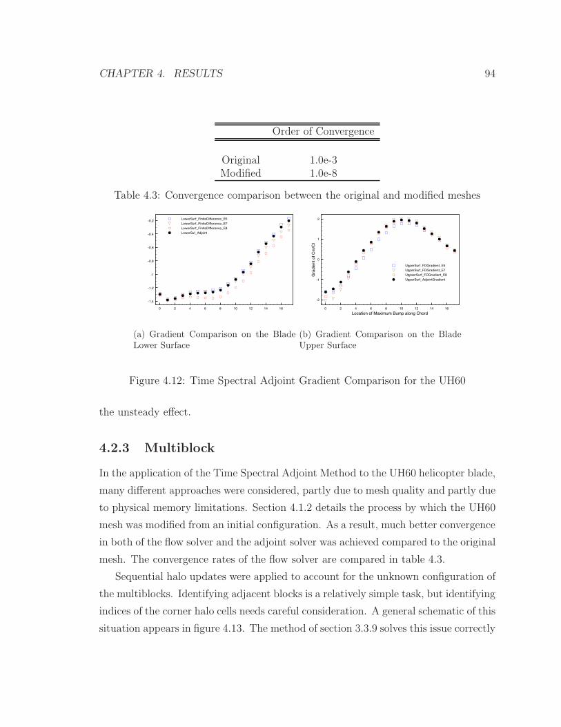
CHAPTER 4. RESULTS 94
Order of Convergence
Original 1.0e-3Modified 1.0e-8
Table 4.3: Convergence comparison between the original and modified meshes
0 2 4 6 8 10 12 14 16
-1.4
-1.2
-1
-0.8
-0.6
-0.4
-0.2LowerSurf_FiniteDifference_E5
LowerSurf_FiniteDifference_E7
LowerSurf_FiniteDifference_E8
LowerSuf_Adjoint
(a) Gradient Comparison on the BladeLower Surface
0 2 4 6 8 10 12 14 16
Location of Maximum Bump along Chord
-2
-1
0
1
2
Gradient of Cm/Cl
UpperSurf_FDGradient_E5
UpperSurf_FDGradient_E7
UppserSurf_FDGradient_E8
UpperSurf_AdjointGradient
(b) Gradient Comparison on the BladeUpper Surface
Figure 4.12: Time Spectral Adjoint Gradient Comparison for the UH60
the unsteady effect.
4.2.3 Multiblock
In the application of the Time Spectral Adjoint Method to the UH60 helicopter blade,
many different approaches were considered, partly due to mesh quality and partly due
to physical memory limitations. Section 4.1.2 details the process by which the UH60
mesh was modified from an initial configuration. As a result, much better convergence
in both of the flow solver and the adjoint solver was achieved compared to the original
mesh. The convergence rates of the flow solver are compared in table 4.3.
Sequential halo updates were applied to account for the unknown configuration of
the multiblocks. Identifying adjacent blocks is a relatively simple task, but identifying
indices of the corner halo cells needs careful consideration. A general schematic of this
situation appears in figure 4.13. The method of section 3.3.9 solves this issue correctly
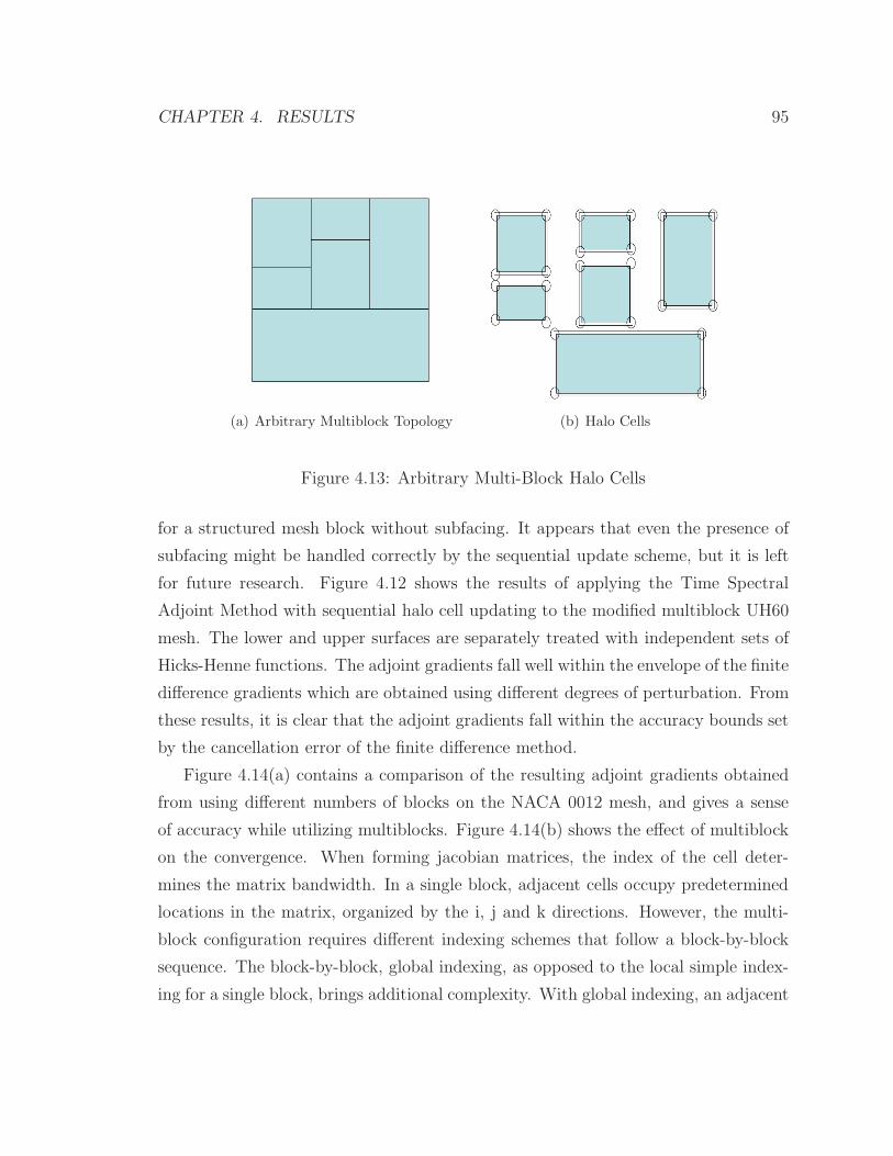
CHAPTER 4. RESULTS 95
(a) Arbitrary Multiblock Topology (b) Halo Cells
Figure 4.13: Arbitrary Multi-Block Halo Cells
for a structured mesh block without subfacing. It appears that even the presence of
subfacing might be handled correctly by the sequential update scheme, but it is left
for future research. Figure 4.12 shows the results of applying the Time Spectral
Adjoint Method with sequential halo cell updating to the modified multiblock UH60
mesh. The lower and upper surfaces are separately treated with independent sets of
Hicks-Henne functions. The adjoint gradients fall well within the envelope of the finite
difference gradients which are obtained using different degrees of perturbation. From
these results, it is clear that the adjoint gradients fall within the accuracy bounds set
by the cancellation error of the finite difference method.
Figure 4.14(a) contains a comparison of the resulting adjoint gradients obtained
from using different numbers of blocks on the NACA 0012 mesh, and gives a sense
of accuracy while utilizing multiblocks. Figure 4.14(b) shows the effect of multiblock
on the convergence. When forming jacobian matrices, the index of the cell deter-
mines the matrix bandwidth. In a single block, adjacent cells occupy predetermined
locations in the matrix, organized by the i, j and k directions. However, the multi-
block configuration requires different indexing schemes that follow a block-by-block
sequence. The block-by-block, global indexing, as opposed to the local simple index-
ing for a single block, brings additional complexity. With global indexing, an adjacent
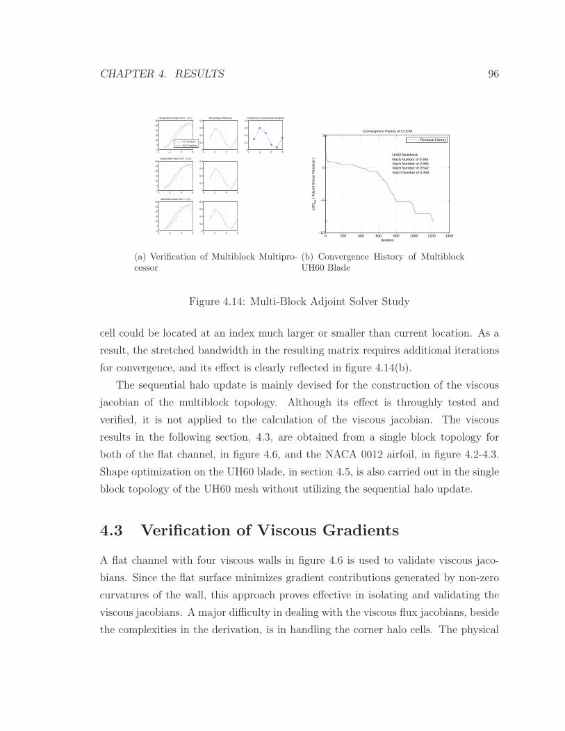
CHAPTER 4. RESULTS 96
0 2 4 60
5
10
15
20
25
30Single Block Single CPU − (1,1)
FD Gradient
ADJ Gradient
0 2 4 60
0.1
0.2
0.3
0.4Percentage Difference
0 2 4 60
0.1
0.2
0.3
0.4Comparison of Normalized Gradient
0 2 4 60
5
10
15
20
25
30Single Block Multi CPU − (1,2)
0 2 4 60
0.1
0.2
0.3
0.4
0 2 4 60
5
10
15
20
25
30Multi Block Multi CPU − (2,2)
0 2 4 60
0.1
0.2
0.3
0.4
(a) Verification of Multiblock Multipro-cessor
0 200 400 600 800 1000 1200 1400−10
−5
0
5Convergence History of CL/CM
Iteration
LOG
10 (
Adj
oint
Sol
ver
Res
idua
l )
UH60 MultiblockMach Number of 0.585Mach Number of 0.885Mach Number of 0.542Mach Number of 0.458
Residual History
(b) Convergence History of MultiblockUH60 Blade
Figure 4.14: Multi-Block Adjoint Solver Study
cell could be located at an index much larger or smaller than current location. As a
result, the stretched bandwidth in the resulting matrix requires additional iterations
for convergence, and its effect is clearly reflected in figure 4.14(b).
The sequential halo update is mainly devised for the construction of the viscous
jacobian of the multiblock topology. Although its effect is throughly tested and
verified, it is not applied to the calculation of the viscous jacobian. The viscous
results in the following section, 4.3, are obtained from a single block topology for
both of the flat channel, in figure 4.6, and the NACA 0012 airfoil, in figure 4.2-4.3.
Shape optimization on the UH60 blade, in section 4.5, is also carried out in the single
block topology of the UH60 mesh without utilizing the sequential halo update.
4.3 Verification of Viscous Gradients
A flat channel with four viscous walls in figure 4.6 is used to validate viscous jaco-
bians. Since the flat surface minimizes gradient contributions generated by non-zero
curvatures of the wall, this approach proves effective in isolating and validating the
viscous jacobians. A major difficulty in dealing with the viscous flux jacobians, beside
the complexities in the derivation, is in handling the corner halo cells. The physical
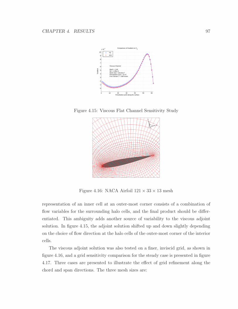
CHAPTER 4. RESULTS 97
0 10 20 30 40 50 60
0
1
2
3
4
5
6
7
8
9
10
x 10−4
Perturbation point along the surface
Gra
dien
t
Comparison of Gradient on Cd
Viscous Channel
Mach = 1.66Re = 1.95e+4Mesh Size = 65x33x17Perturbation Size = 1e−8Free Stream T = 288 Kelvin
FD
ADJ
Figure 4.15: Viscous Flat Channel Sensitivity Study
X
Y
Z
Figure 4.16: NACA Airfoil 121 × 33 × 13 mesh
representation of an inner cell at an outer-most corner consists of a combination of
flow variables for the surrounding halo cells, and the final product should be differ-
entiated. This ambiguity adds another source of variability to the viscous adjoint
solution. In figure 4.15, the adjoint solution shifted up and down slightly depending
on the choice of flow direction at the halo cells of the outer-most corner of the interior
cells.
The viscous adjoint solution was also tested on a finer, inviscid grid, as shown in
figure 4.16, and a grid sensitivity comparison for the steady case is presented in figure
4.17. Three cases are presented to illustrate the effect of grid refinement along the
chord and span directions. The three mesh sizes are:
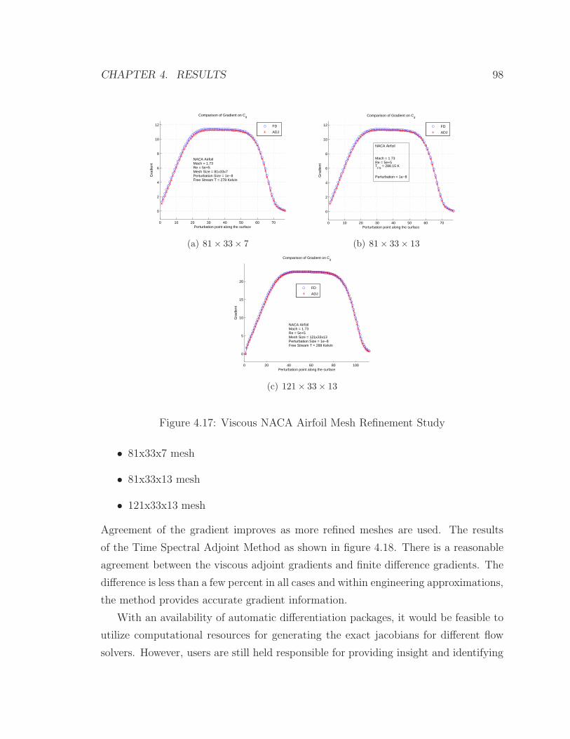
CHAPTER 4. RESULTS 98
0 10 20 30 40 50 60 70
0
2
4
6
8
10
12
Perturbation point along the surface
Gra
dien
t
Comparison of Gradient on Cd
NACA AirfoilMach = 1.73Re = 5e+5Mesh Size = 81x33x7Perturbation Size = 1e−8Free Stream T = 278 Kelvin
FD
ADJ
(a) 81 × 33 × 7
0 10 20 30 40 50 60 70
0
2
4
6
8
10
12
Perturbation point along the surface
Gra
dien
t
Comparison of Gradient on Cd
FD
ADJ
NACA Airfoil
Mach = 1.73Re = 5e+5T
FS = 288.15 K
Perturbation = 1e−8
(b) 81 × 33 × 13
0 20 40 60 80 100
0
5
10
15
20
Perturbation point along the surface
Gra
dien
t
Comparison of Gradient on Cd
NACA AirfoilMach = 1.73Re = 5e+5Mesh Size = 121x33x13Perturbation Size = 1e−8Free Stream T = 288 Kelvin
FD
ADJ
(c) 121 × 33 × 13
Figure 4.17: Viscous NACA Airfoil Mesh Refinement Study
• 81x33x7 mesh
• 81x33x13 mesh
• 121x33x13 mesh
Agreement of the gradient improves as more refined meshes are used. The results
of the Time Spectral Adjoint Method as shown in figure 4.18. There is a reasonable
agreement between the viscous adjoint gradients and finite difference gradients. The
difference is less than a few percent in all cases and within engineering approximations,
the method provides accurate gradient information.
With an availability of automatic differentiation packages, it would be feasible to
utilize computational resources for generating the exact jacobians for different flow
solvers. However, users are still held responsible for providing insight and identifying
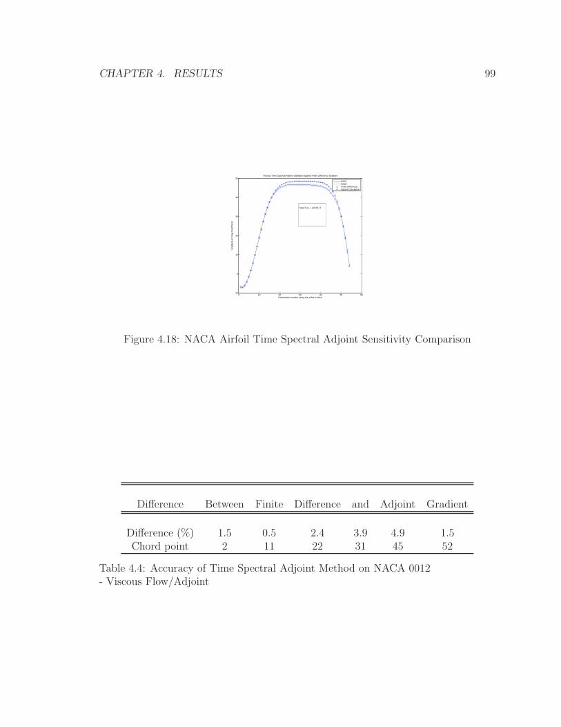
CHAPTER 4. RESULTS 99
0 10 20 30 40 50 60−10
0
10
20
30
40
50
Pertubation location along the airfoil surface
Gra
dien
t on
Dra
g C
oeffi
cien
t
Viscous Time Spectral Adjoint Validation against Finite Difference Gradient
data1data2Finite DifferenceAdjoint Calculation
Step Size = 1.8x10⁻⁴
Figure 4.18: NACA Airfoil Time Spectral Adjoint Sensitivity Comparison
Difference Between Finite Difference and Adjoint Gradient
Difference (%) 1.5 0.5 2.4 3.9 4.9 1.5Chord point 2 11 22 31 45 52
Table 4.4: Accuracy of Time Spectral Adjoint Method on NACA 0012- Viscous Flow/Adjoint
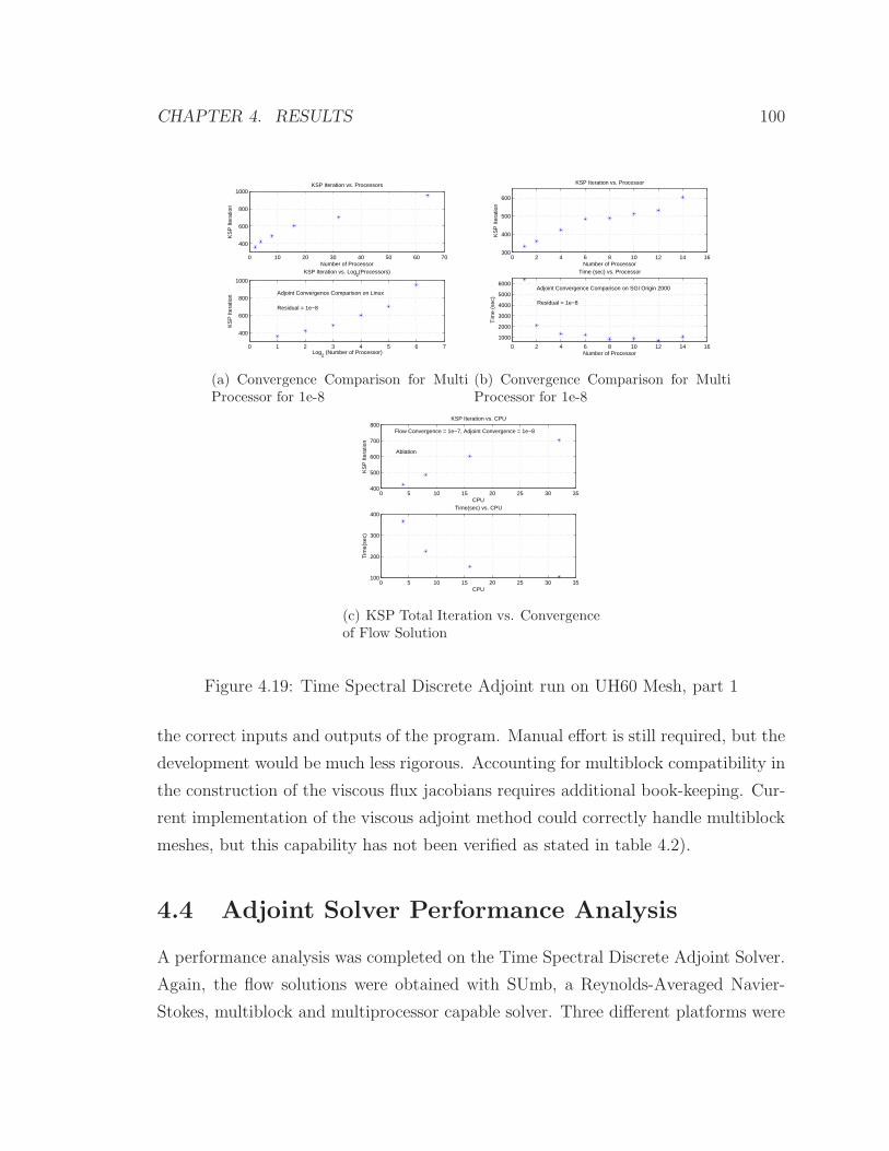
CHAPTER 4. RESULTS 100
0 10 20 30 40 50 60 70
400
600
800
1000KSP Iteration vs. Processors
Number of Processor
KS
P It
erat
ion
0 1 2 3 4 5 6 7
400
600
800
1000
KSP Iteration vs. Log2(Processors)
Log2 (Number of Processor)
KS
P It
erat
ion Adjoint Convergence Comparison on Linux
Residual = 1e−8
(a) Convergence Comparison for MultiProcessor for 1e-8
0 2 4 6 8 10 12 14 16300
400
500
600
KSP Iteration vs. Processor
Number of Processor
KS
P It
erat
ion
0 2 4 6 8 10 12 14 16
1000
2000
3000
4000
5000
6000
Time (sec) vs. Processor
Number of Processor
Tim
e (s
ec)
Adjoint Convergence Comparison on SGI Origin 2000
Residual = 1e−8
(b) Convergence Comparison for MultiProcessor for 1e-8
0 5 10 15 20 25 30 35400
500
600
700
800KSP Iteration vs. CPU
CPU
KS
P It
erat
ion
Flow Convergence = 1e−7, Adjoint Convergence = 1e−8
Ablation
0 5 10 15 20 25 30 35100
200
300
400Time(sec) vs. CPU
CPU
Tim
e(se
c)
(c) KSP Total Iteration vs. Convergenceof Flow Solution
Figure 4.19: Time Spectral Discrete Adjoint run on UH60 Mesh, part 1
the correct inputs and outputs of the program. Manual effort is still required, but the
development would be much less rigorous. Accounting for multiblock compatibility in
the construction of the viscous flux jacobians requires additional book-keeping. Cur-
rent implementation of the viscous adjoint method could correctly handle multiblock
meshes, but this capability has not been verified as stated in table 4.2).
4.4 Adjoint Solver Performance Analysis
A performance analysis was completed on the Time Spectral Discrete Adjoint Solver.
Again, the flow solutions were obtained with SUmb, a Reynolds-Averaged Navier-
Stokes, multiblock and multiprocessor capable solver. Three different platforms were
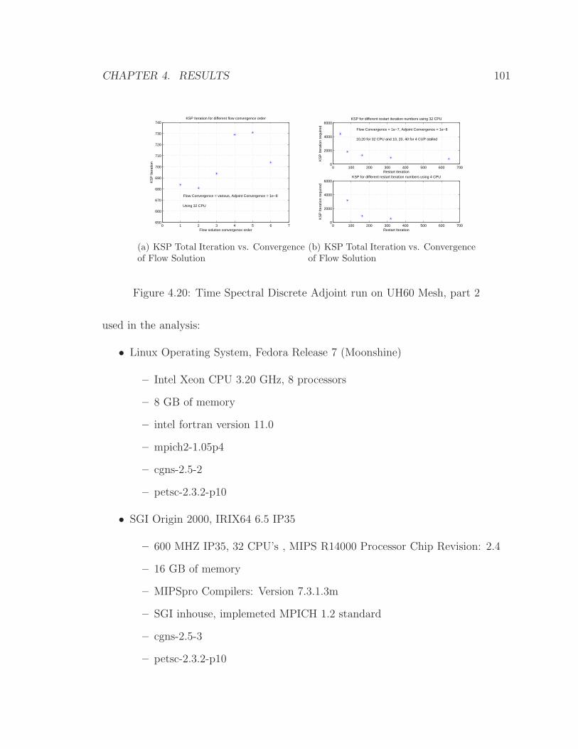
CHAPTER 4. RESULTS 101
0 1 2 3 4 5 6 7650
660
670
680
690
700
710
720
730
740KSP Iteration for different flow convergence order
Flow solution convergence order
KS
P It
erat
ion
Flow Convergence = various, Adjoint Convergence = 1e−8
Using 32 CPU
(a) KSP Total Iteration vs. Convergenceof Flow Solution
0 100 200 300 400 500 600 7000
2000
4000
6000KSP for different restart iteration numbers using 32 CPU
Restart Iteration
KS
P It
erat
ion
requ
ired
Flow Convergence = 1e−7, Adjoint Convergence = 1e−8
10,20 for 32 CPU and 10, 20, 40 for 4 CUP stalled
0 100 200 300 400 500 600 7000
2000
4000
6000KSP for different restart iteration numbers using 4 CPU
Restart Iteration
KS
P It
erat
ion
requ
ired
(b) KSP Total Iteration vs. Convergenceof Flow Solution
Figure 4.20: Time Spectral Discrete Adjoint run on UH60 Mesh, part 2
used in the analysis:
• Linux Operating System, Fedora Release 7 (Moonshine)
– Intel Xeon CPU 3.20 GHz, 8 processors
– 8 GB of memory
– intel fortran version 11.0
– mpich2-1.05p4
– cgns-2.5-2
– petsc-2.3.2-p10
• SGI Origin 2000, IRIX64 6.5 IP35
– 600 MHZ IP35, 32 CPU’s , MIPS R14000 Processor Chip Revision: 2.4
– 16 GB of memory
– MIPSpro Compilers: Version 7.3.1.3m
– SGI inhouse, implemeted MPICH 1.2 standard
– cgns-2.5-3
– petsc-2.3.2-p10
CHAPTER 4. RESULTS 102
• Ablation, Centos
– Itainium, 96 processors
– 2 GB per processor
– Intel compiler
– mpich2
– cgns-2.5-3
– petsc-2.3.2-p10
The analysis was performed on the UH60 rotor blade running in parallel on multiple
processors. A single block topology was chosen rather than multiblock, and the com-
munication of the processors was achieved through the SUmb native communication
channel. Figure 4.19 shows the variation in the number of iterations and CPU time
required for a given level of convergence as the number of processors is changed. KSP
Iteration in the figure refers to the total number of iterations required for convergence
with PETSc. Figure 4.20 also shows variations in the iteration number, using various
restart numbers and various orders of convergence for the flow solution.
First, a study was performed to determine the number of iterations PETSc requires
to achieve a minimum residual of 1e−8. On the linux machine, the study was carried
out for 2, 4, 8, 16, 32 and 64 processors. The linux box only has eight CPU’s. However,
for the purpose of measuring the number of iteration, not the actual run time, the
given configuration produces meaningful results. Figure 4.19(a), on the linux box,
shows two plots of the results obtained using up to 64 processors. The second plot
simply took the logarithm on both axes, so that more features can be revealed, if
present. It does show slightly exponential or parabolic patterns. Figure 4.19(b), on
the SGI, used 1, 2, 4, 6, 8, 10, 12 and 14 processors. This figure also compares the
convergence time for different numbers of processors. It shows a dramatic reduction
in CPU time from one processor to two processors and a slightly inverse relationship
between the CPU time and the processor count can be spotted throughout the entire
plot. The total run time has plateaued around 1000 iterations, which signifies a
tradeoff between the number of processors and the overhead cost of communication.
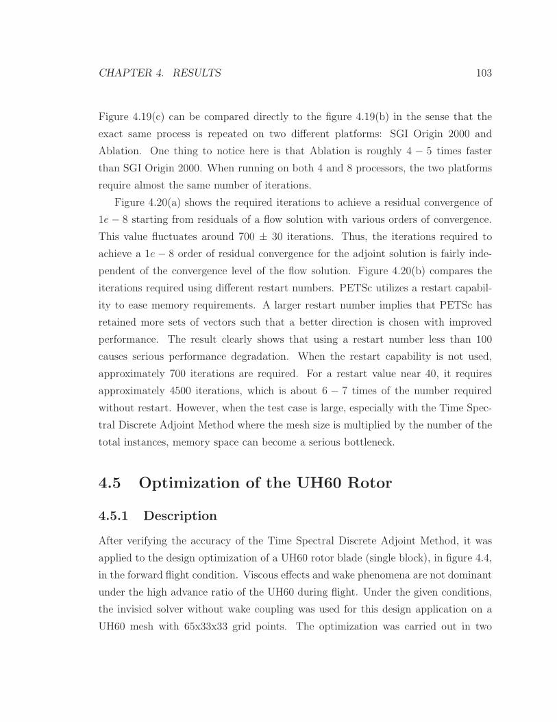
CHAPTER 4. RESULTS 103
Figure 4.19(c) can be compared directly to the figure 4.19(b) in the sense that the
exact same process is repeated on two different platforms: SGI Origin 2000 and
Ablation. One thing to notice here is that Ablation is roughly 4 − 5 times faster
than SGI Origin 2000. When running on both 4 and 8 processors, the two platforms
require almost the same number of iterations.
Figure 4.20(a) shows the required iterations to achieve a residual convergence of
1e − 8 starting from residuals of a flow solution with various orders of convergence.
This value fluctuates around 700 ± 30 iterations. Thus, the iterations required to
achieve a 1e − 8 order of residual convergence for the adjoint solution is fairly inde-
pendent of the convergence level of the flow solution. Figure 4.20(b) compares the
iterations required using different restart numbers. PETSc utilizes a restart capabil-
ity to ease memory requirements. A larger restart number implies that PETSc has
retained more sets of vectors such that a better direction is chosen with improved
performance. The result clearly shows that using a restart number less than 100
causes serious performance degradation. When the restart capability is not used,
approximately 700 iterations are required. For a restart value near 40, it requires
approximately 4500 iterations, which is about 6 − 7 times of the number required
without restart. However, when the test case is large, especially with the Time Spec-
tral Discrete Adjoint Method where the mesh size is multiplied by the number of the
total instances, memory space can become a serious bottleneck.
4.5 Optimization of the UH60 Rotor
4.5.1 Description
After verifying the accuracy of the Time Spectral Discrete Adjoint Method, it was
applied to the design optimization of a UH60 rotor blade (single block), in figure 4.4,
in the forward flight condition. Viscous effects and wake phenomena are not dominant
under the high advance ratio of the UH60 during flight. Under the given conditions,
the invisicd solver without wake coupling was used for this design application on a
UH60 mesh with 65x33x33 grid points. The optimization was carried out in two
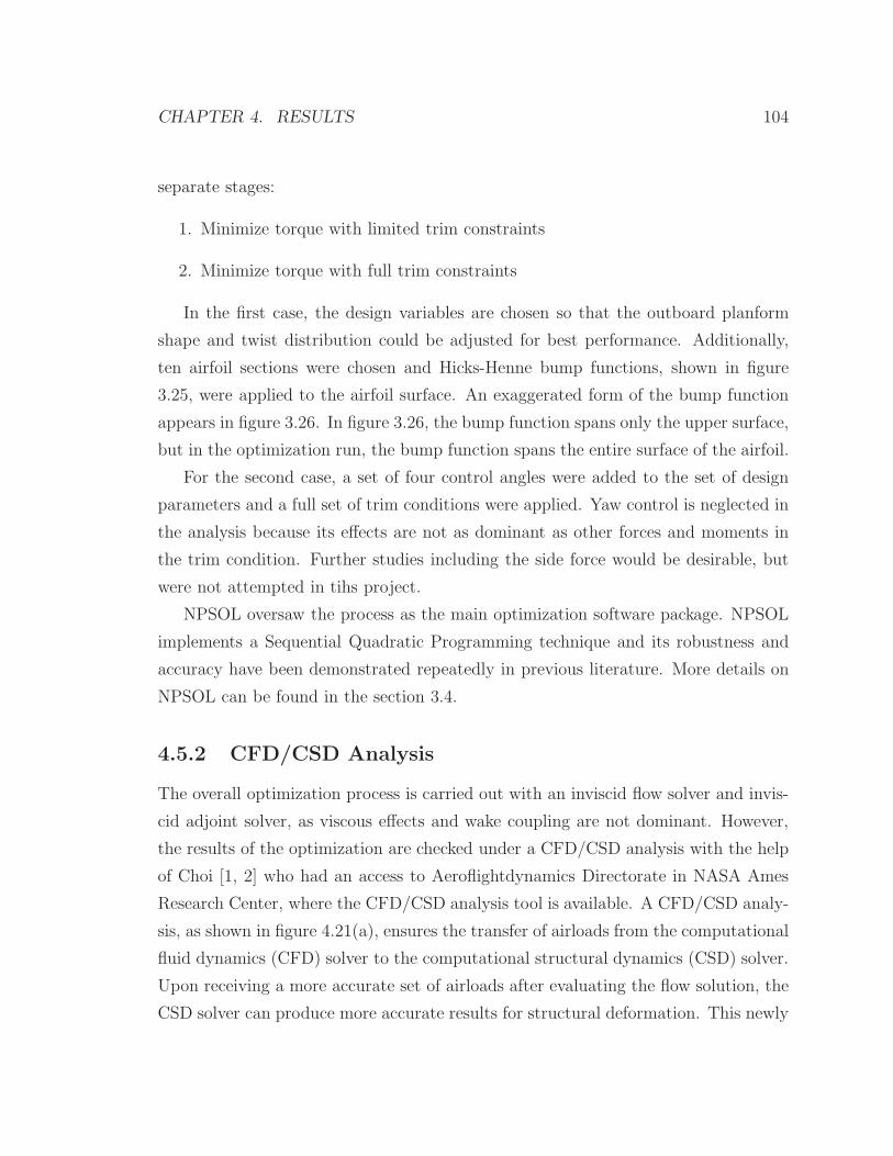
CHAPTER 4. RESULTS 104
separate stages:
1. Minimize torque with limited trim constraints
2. Minimize torque with full trim constraints
In the first case, the design variables are chosen so that the outboard planform
shape and twist distribution could be adjusted for best performance. Additionally,
ten airfoil sections were chosen and Hicks-Henne bump functions, shown in figure
3.25, were applied to the airfoil surface. An exaggerated form of the bump function
appears in figure 3.26. In figure 3.26, the bump function spans only the upper surface,
but in the optimization run, the bump function spans the entire surface of the airfoil.
For the second case, a set of four control angles were added to the set of design
parameters and a full set of trim conditions were applied. Yaw control is neglected in
the analysis because its effects are not as dominant as other forces and moments in
the trim condition. Further studies including the side force would be desirable, but
were not attempted in tihs project.
NPSOL oversaw the process as the main optimization software package. NPSOL
implements a Sequential Quadratic Programming technique and its robustness and
accuracy have been demonstrated repeatedly in previous literature. More details on
NPSOL can be found in the section 3.4.
4.5.2 CFD/CSD Analysis
The overall optimization process is carried out with an inviscid flow solver and invis-
cid adjoint solver, as viscous effects and wake coupling are not dominant. However,
the results of the optimization are checked under a CFD/CSD analysis with the help
of Choi [1, 2] who had an access to Aeroflightdynamics Directorate in NASA Ames
Research Center, where the CFD/CSD analysis tool is available. A CFD/CSD analy-
sis, as shown in figure 4.21(a), ensures the transfer of airloads from the computational
fluid dynamics (CFD) solver to the computational structural dynamics (CSD) solver.
Upon receiving a more accurate set of airloads after evaluating the flow solution, the
CSD solver can produce more accurate results for structural deformation. This newly
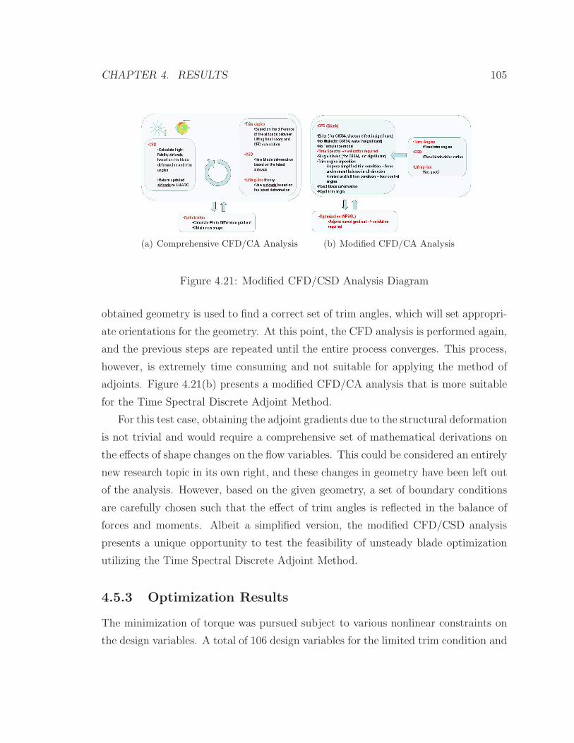
CHAPTER 4. RESULTS 105
(a) Comprehensive CFD/CA Analysis (b) Modified CFD/CA Analysis
Figure 4.21: Modified CFD/CSD Analysis Diagram
obtained geometry is used to find a correct set of trim angles, which will set appropri-
ate orientations for the geometry. At this point, the CFD analysis is performed again,
and the previous steps are repeated until the entire process converges. This process,
however, is extremely time consuming and not suitable for applying the method of
adjoints. Figure 4.21(b) presents a modified CFD/CA analysis that is more suitable
for the Time Spectral Discrete Adjoint Method.
For this test case, obtaining the adjoint gradients due to the structural deformation
is not trivial and would require a comprehensive set of mathematical derivations on
the effects of shape changes on the flow variables. This could be considered an entirely
new research topic in its own right, and these changes in geometry have been left out
of the analysis. However, based on the given geometry, a set of boundary conditions
are carefully chosen such that the effect of trim angles is reflected in the balance of
forces and moments. Albeit a simplified version, the modified CFD/CSD analysis
presents a unique opportunity to test the feasibility of unsteady blade optimization
utilizing the Time Spectral Discrete Adjoint Method.
4.5.3 Optimization Results
The minimization of torque was pursued subject to various nonlinear constraints on
the design variables. A total of 106 design variables for the limited trim condition and
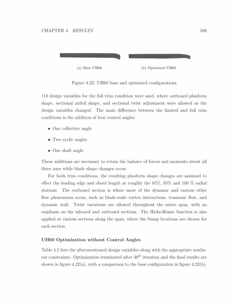
CHAPTER 4. RESULTS 106
(a) Base UH60 (b) Optimized UH60
Figure 4.22: UH60 base and optimized configurations
110 design variables for the full trim condition were used, where outboard planform
shape, sectional airfoil shape, and sectional twist adjustment were allowed as the
design variables changed. The main difference between the limited and full trim
conditions is the addition of four control angles:
• One collective angle
• Two cyclic angles
• One shaft angle
These additions are necessary to retain the balance of forces and moments about all
three axes while blade shape changes occur.
For both trim conditions, the resulting planform shape changes are assumed to
effect the leading edge and chord length at roughly the 85%, 95% and 100 % radial
stations. The outboard section is where most of the dynamic and various other
flow phenomena occur, such as blade-wake vortex interactions, transonic flow, and
dynamic stall. Twist variations are allowed throughout the entire span, with an
emphasis on the inboard and outboard sections. The Hicks-Henne function is also
applied at various sections along the span, where the bump locations are chosen for
each section.
UH60 Optimization without Control Angles
Table 4.5 lists the aforementioned design variables along with the appropriate nonlin-
ear constraints. Optimization terminated after 38th iteration and the final results are
shown in figure 4.22(a), with a comparison to the base configuration in figure 4.22(b).
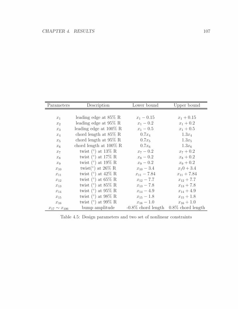
CHAPTER 4. RESULTS 107
Parameters Description Lower bound Upper bound
x1 leading edge at 85% R x1 − 0.15 x1 + 0.15x2 leading edge at 95% R x1 − 0.2 x1 + 0.2x3 leading edge at 100% R x1 − 0.5 x1 + 0.5x4 chord length at 85% R 0.7x4 1.3x4
x5 chord length at 95% R 0.7x5 1.3x5
x6 chord length at 100% R 0.7x6 1.3x6
x7 twist () at 13% R x7 − 0.2 x7 + 0.2x8 twist () at 17% R x8 − 0.2 x8 + 0.2x9 twist () at 19% R x9 − 0.2 x9 + 0.2x10 twist() at 26% R x10 − 3.4 x10 + 3.4x11 twist () at 42% R x11 − 7.84 x11 + 7.84x12 twist () at 65% R x12 − 7.7 x12 + 7.7x13 twist () at 85% R x13 − 7.8 x13 + 7.8x14 twist () at 95% R x14 − 4.9 x14 + 4.9x15 twist () at 98% R x15 − 1.8 x15 + 1.8x16 twist () at 99% R x16 − 1.0 x16 + 1.0
x17 ∼ x106 bump amplitude -0.8% chord length 0.8% chord length
Table 4.5: Design parameters and two set of nonlinear constraints
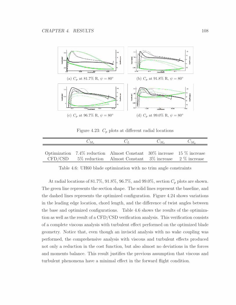
CHAPTER 4. RESULTS 108
(a) Cp at 81.7% R, ψ = 80 (b) Cp at 91.8% R, ψ = 80
(c) Cp at 96.7% R, ψ = 80 (d) Cp at 99.0% R, ψ = 80
Figure 4.23: Cp plots at different radial locations
CMzCL CMx
CMy
Optimization 7.4% reduction Almost Constant 30% increase 15 % increaseCFD/CSD 5% reduction Almost Constant 3% increase 2 % increase
Table 4.6: UH60 blade optimization with no trim angle constraints
At radial locations of 81.7%, 91.8%, 96.7%, and 99.0%, section Cp plots are shown.
The green line represents the section shape. The solid lines represent the baseline, and
the dashed lines represents the optimized configuration. Figure 4.24 shows variations
in the leading edge location, chord length, and the difference of twist angles between
the base and optimized configurations. Table 4.6 shows the results of the optimiza-
tion as well as the result of a CFD/CSD verification analysis. This verification consists
of a complete viscous analysis with turbulent effect performed on the optimized blade
geometry. Notice that, even though an inviscid analysis with no wake coupling was
performed, the comprehensive analysis with viscous and turbulent effects produced
not only a reduction in the cost function, but also almost no deviations in the forces
and moments balance. This result justifies the previous assumption that viscous and
turbulent phenomena have a minimal effect in the forward flight condition.
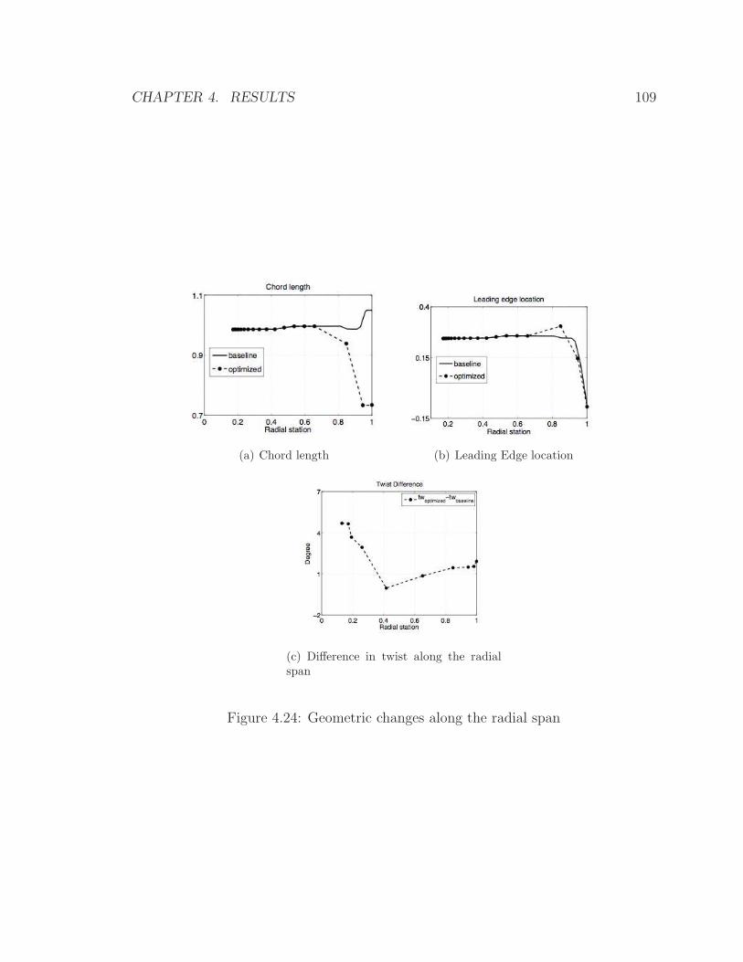
CHAPTER 4. RESULTS 109
(a) Chord length (b) Leading Edge location
(c) Difference in twist along the radialspan
Figure 4.24: Geometric changes along the radial span
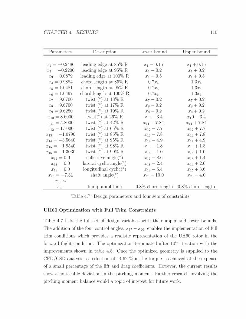
CHAPTER 4. RESULTS 110
Parameters Description Lower bound Upper bound
x1 = −0.2486 leading edge at 85% R x1 − 0.15 x1 + 0.15x2 = −0.2200 leading edge at 95% R x1 − 0.2 x1 + 0.2x3 = 0.0879 leading edge at 100% R x1 − 0.5 x1 + 0.5x4 = 0.9884 chord length at 85% R 0.7x4 1.3x4
x5 = 1.0481 chord length at 95% R 0.7x5 1.3x5
x6 = 1.0497 chord length at 100% R 0.7x6 1.3x6
x7 = 9.6700 twist () at 13% R x7 − 0.2 x7 + 0.2x8 = 9.6700 twist () at 17% R x8 − 0.2 x8 + 0.2x9 = 9.6280 twist () at 19% R x9 − 0.2 x9 + 0.2x10 = 8.6000 twist() at 26% R x10 − 3.4 x10 + 3.4x11 = 5.8000 twist () at 42% R x11 − 7.84 x11 + 7.84x12 = 1.7000 twist () at 65% R x12 − 7.7 x12 + 7.7x13 = −1.0790 twist () at 85% R x13 − 7.8 x13 + 7.8x14 = −3.5640 twist () at 95% R x14 − 4.9 x14 + 4.9x15 = −1.9540 twist () at 98% R x15 − 1.8 x15 + 1.8x16 = −1.3030 twist () at 99% R x16 − 1.0 x16 + 1.0x17 = 0.0 collective angle() x17 − 8.6 x13 + 1.4x18 = 0.0 lateral cyclic angle() x18 − 2.4 x14 + 2.6x19 = 0.0 longitudinal cyclic() x19 − 6.4 x15 + 3.6x20 = −7.31 shaft angle() x20 − 10.0 x20 − 4.0
x21 ∼x110 bump amplitude -0.8% chord length 0.8% chord length
Table 4.7: Design parameters and four sets of constraints
UH60 Optimization with Full Trim Constraints
Table 4.7 lists the full set of design variables with their upper and lower bounds.
The addition of the four control angles, x17 − x20, enables the implementation of full
trim conditions which provides a realistic representation of the UH60 rotor in the
forward flight condition. The optimization terminated after 10th iteration with the
improvements shown in table 4.8. Once the optimized geometry is supplied to the
CFD/CSD analysis, a reduction of 14.62 % in the torque is achieved at the expense
of a small percentage of the lift and drag coefficients. However, the current results
show a noticeable deviation in the pitching moment. Further research involving the
pitching moment balance would a topic of interest for future work.
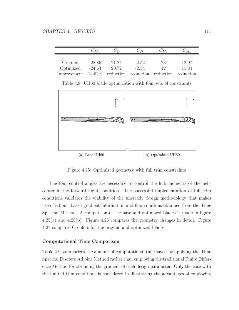
CHAPTER 4. RESULTS 111
CMzCL CD CMx
CMy
Original -28.86 21.24 -2.52 23 12.97Optimized -24.64 20.72 -2.34 12 11.34
Improvement 14.62% reduction reduction reduction reduction
Table 4.8: UH60 blade optimization with four sets of constraints
(a) Base UH60 (b) Optimized UH60
Figure 4.25: Optimized geometry with full trim constraints
The four control angles are necessary to control the hub moments of the heli-
copter in the forward flight condition. The successful implementation of full trim
conditions validates the viability of the unsteady design methodology that makes
use of adjoint-based gradient information and flow solutions obtained from the Time
Spectral Method. A comparison of the base and optimized blades is made in figure
4.25(a) and 4.25(b). Figure 4.26 compares the geometry changes in detail. Figure
4.27 compares Cp plots for the original and optimized blades.
Computational Time Comparison
Table 4.9 summarizes the amount of computational time saved by applying the Time
Spectral Discrete Adjoint Method rather than employing the traditional Finite Differ-
ence Method for obtaining the gradient of each design parameter. Only the case with
the limited trim conditions is considered in illustrating the advantages of employing
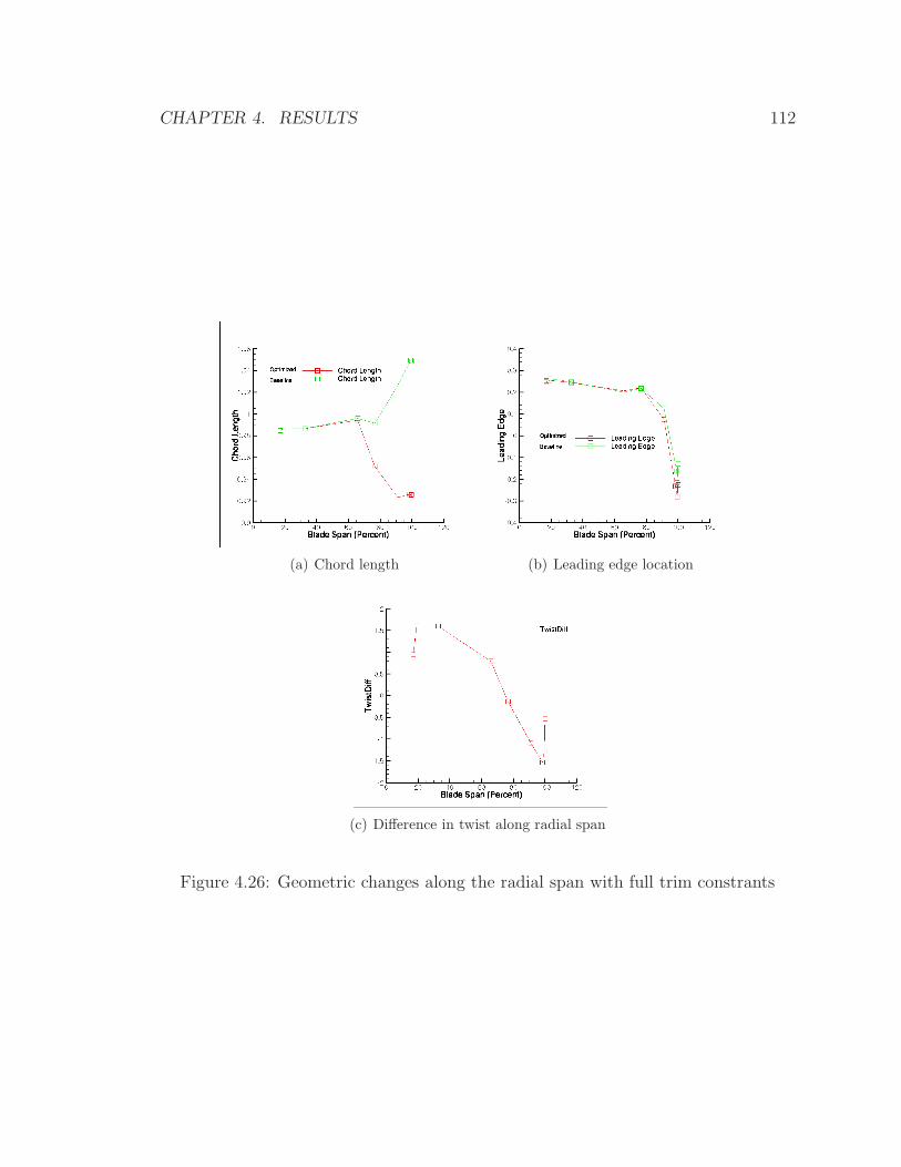
CHAPTER 4. RESULTS 112
(a) Chord length (b) Leading edge location
(c) Difference in twist along radial span
Figure 4.26: Geometric changes along the radial span with full trim constrants
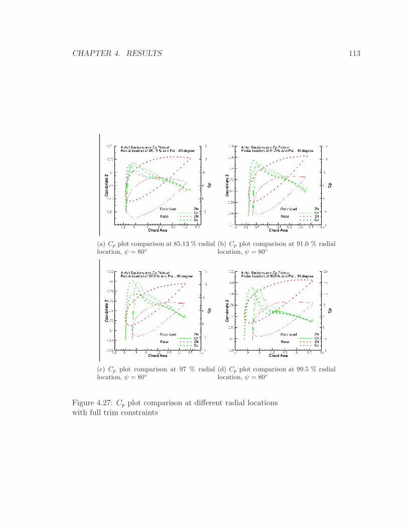
CHAPTER 4. RESULTS 113
(a) Cp plot comparison at 85.13 % radiallocation, ψ = 80
(b) Cp plot comparison at 91.0 % radiallocation, ψ = 80
(c) Cp plot comparison at 97 % radiallocation, ψ = 80
(d) Cp plot comparison at 99.5 % radiallocation, ψ = 80
Figure 4.27: Cp plot comparison at different radial locationswith full trim constraints
CHAPTER 4. RESULTS 114
the Time Spectral Adjoint methodology for unsteady optimization.
For each design parameter, the finite difference gradient must be calculated at
each design point, whereas the adjoint gradients can be determined for all param-
eters simultaneously at each design point. The cost associated with the adjoint
method is therefore equivalent to having a single parameter. As an example, with
finite difference gradients and a residual convergence of 1e − 6, it would require
5185.4 ∗ 100 sec = 144 hours per iteration for solving a flow solution 100 times. For
38 iterations, it would take 144 hours ∗ 38 iterations = 228 days , and this is just to
complete the unsteady design. In summary, by using adjoint gradients, 4.5 days of
computational time would be enough for 100 design parameters and 38 iterations for
what would have taken 228 days of CPU time with finite difference gradients. Not
only does it save tremendous amount of computational time, but the new method-
ology is solely responsible for making computationally infeasible problem completely
tractable.
Table 4.10 contains a run time comparison for the NACA0012 airfoil. Optimiza-
tion was not performed, but listed is the computational time that could be saved if
the optimization is to be carried out. Again, not only does it save almost 98% of the
CPU time, it enables computation that was previously not possible.
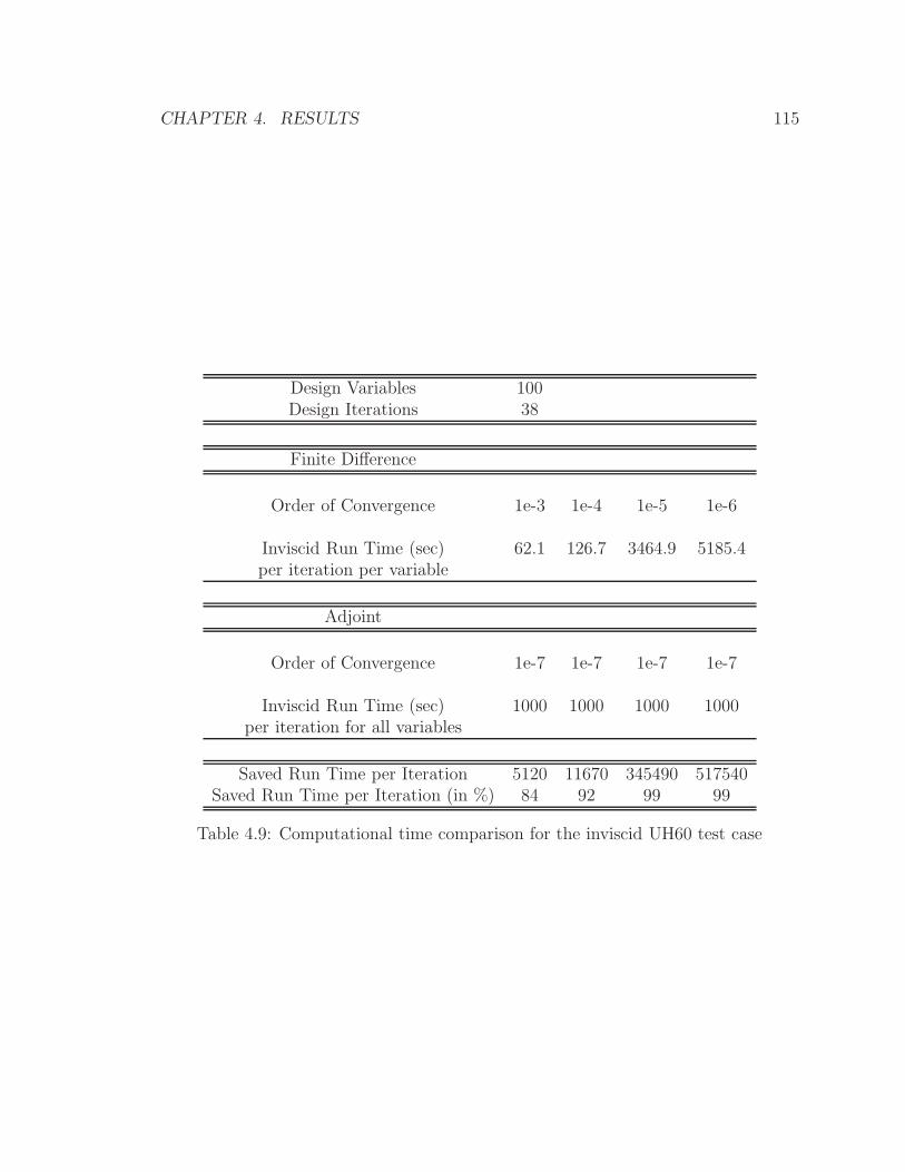
CHAPTER 4. RESULTS 115
Design Variables 100Design Iterations 38
Finite Difference
Order of Convergence 1e-3 1e-4 1e-5 1e-6
Inviscid Run Time (sec) 62.1 126.7 3464.9 5185.4per iteration per variable
Adjoint
Order of Convergence 1e-7 1e-7 1e-7 1e-7
Inviscid Run Time (sec) 1000 1000 1000 1000per iteration for all variables
Saved Run Time per Iteration 5120 11670 345490 517540Saved Run Time per Iteration (in %) 84 92 99 99
Table 4.9: Computational time comparison for the inviscid UH60 test case
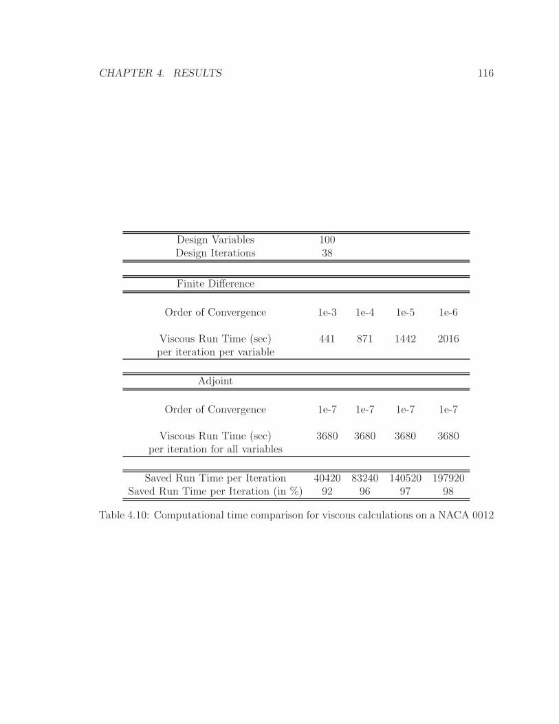
CHAPTER 4. RESULTS 116
Design Variables 100Design Iterations 38
Finite Difference
Order of Convergence 1e-3 1e-4 1e-5 1e-6
Viscous Run Time (sec) 441 871 1442 2016per iteration per variable
Adjoint
Order of Convergence 1e-7 1e-7 1e-7 1e-7
Viscous Run Time (sec) 3680 3680 3680 3680per iteration for all variables
Saved Run Time per Iteration 40420 83240 140520 197920Saved Run Time per Iteration (in %) 92 96 97 98
Table 4.10: Computational time comparison for viscous calculations on a NACA 0012
Chapter 5
Conclusions & Future Work
5.1 Conclusions
Unsteady flows in nature appear in numerous forms: flapping wings, turbulence,
turbomachinery flows, rotating stall, and surge, just to name a few. In engineering
sysystem, unsteady phenomena, not only shorten the life-cycle of the components,
but also may lead to operational failures which cost human lives. Consequenty, there
has been an enormous need for the ability to perform optimization in unsteady flows,
but due to the difficulties in implementation, only a minimal amount work has been
carried out so far. In this thesis, an unsteady optimization methodology utilizing
adjoint-based gradients along with the Time Spectral Method for periodic flows has
been implemented and validated.
Traditionally, many developed algorithms have contributed to solving unsteady
flows. Starting from explicit methods, which include Runge-Kutta and various other
multi-step methods, all the way to implicit methods, which include ADI, DD-ADI and
BDF, many algorithms have been applied to unsteady optimization. Most explicit
schemes face the problem of traversing through a large number of time steps. The
problem is aggravated by the presence of transient solutions, which tend to grow
longer for flows with high frequency components, such as high-RPM compressors.
Implicit algorithms often face storage problems, as well. High-order models such as
the Nonlinear Frequency Domain Method and the Harmonic Balance Method have
117
CHAPTER 5. CONCLUSIONS & FUTURE WORK 118
been applied to bypass transient solutions, but the computational time spent on
converting variables between the time and frequency domains has proved to be quite
significant. The extra storage space required for complex variables also presents an
additional problem. In a typical unsteady optimization process, with each design
iteration, the optimizer requires gradient information which is obtained by solving
the unsteady flow equations as many times as the number of design parameters plus
one. But with adjoint gradients based on the time spectral flow solutions, the number
of required unsteady flow evaluations is reduced to two: one for solving the unsteady
flow around the current geometry and the other for solving the adjoint equation with
perturbations applied to a set of design parameters. As a result, the Time Spectral
Adjoint Method provides gradient information with such a low computational cost
that it enables optimization within certain categories of periodic unsteady flows that
have not been previously attempted.
The unsteady adjoint gradient method proposes a way to obtain gradient infor-
mation at low computational cost at a given design iteration. However, since the
adjoint requires backward integration in time, the entire flow solution at every time
step needs to be stored. A typical number of time steps in an engineering application
might range between a few hundred to tens of thousands, which renders the storage
of the entire flow solution very problematic. Using adjoint gradients with the Time
Spectral Method for unsteady flows with periodicity solves not only the storage prob-
lem, but also bypasses the time required to step through transient solutions. Entire
periodic flow solutions are solved at once.
Finally, this research proposed, implemented, and validated a design methodology
for unsteady flows with periodicity. It has been tested on a NACA 0012 airfoil ex-
tensively, and upon a validation of the adjoint implementation, it was applied to the
design optimization of a UH60 blade in forward flight with trim conditions. Along
the development timeline, a partial set of trim conditions were applied first to the
optimization process, which resulted in 5 % improvement in torque. A full set of trim
condition were also applied, resulting in a 14.6 % improvement, but at the expense of
violating the moment balance. Both cases demonstrated improvements after applying
a CFD/CA analysis (cowork with Choi).
CHAPTER 5. CONCLUSIONS & FUTURE WORK 119
The successful implementation and verification of the proposed design methodol-
ogy opens up many areas of engineering applications. Flutter often shortens the life
expectancy of an aircraft wing or other components. Rotating stall in a compressor
not only damages the compressor blades, but also exposes humans to serious danger
during engine failure events. Turbulent flows also exhibit periodicity. From flapping
bird wings to the engine cycle of a car, there are numerous examples of periodic,
unsteady flows in nature and the Time Spectral Adjoint approach would be a good
starting point for tackling these problems.
As a final list of technical developments in this thesis, the following concepts were
derived, implemented and validated:
• Euler flux jacobians for discrete adjoints
• Artificial viscosity jacobians
• Viscous flux jacobian
• Various boundary conditions
– Farfield
– Supersonic Inlet/Outlet
– Subsonic Inlet/Outlet
– Euler wall
– Viscous wall
– Symmetric wall
– Internal 1-to-1
• Multi-processor capability using MPI and PETSc
• Multi-block capability through a Sequential Halo Update procedure.
CHAPTER 5. CONCLUSIONS & FUTURE WORK 120
5.2 Future Work
Adjoint solutions, mostly used to obtain gradient information, can also provide an
error indicator without any additional computational cost. Mesh quality becomes
one of the primary factors that helps to achieve a faster flow convergence. However,
a better quality grid requires longer computational times. In time spectral solutions,
the total number of grid points is multiplied by the number of total time instances, so
that the final run time is prolonged by the same multiplicative factor. Error indicators
could be used to redistribute or refine the mesh in the areas where a reduction of error
is maximized with a minimum amount of mesh modification.
The application of unsteady optimization to a turbomachinery flow would be a
good example, as well. An advantage of using discrete adjoints is that it allows the
selection of any flow quantity for the cost function, so optimization could be applied
to quantities such as the total pressure loss across the compressor or the prevention
of surge under given conditions.
The addition of different trim conditions to the UH60 test case would be a useful
exercise. With the successful implementation of the current optimization methodol-
ogy, comparing optimization results over various trim conditions could present phys-
ical insights that would otherwise hard to obtain.
Flutter could be another useful application. Much research has already been done
on the subject and a great deal of information is available. Utilizing this knowledge
in the context of the Time Spectral Adjoint optimization methodology could provide
wing shapes that are beyond the scope of current physical insight.
Appendix A
Optimization
Optimization problems can be divided into three categories[48, 9]: constrained linear,
unconstrained , and constrained nonlinear optimization. Problems with a linear ob-
jective function fall under linear programming and those with a nonlinear objective
function fall under nonlinear programming. Most of the objective functions, CL, CM ,
and CP and their variants fall under the nonlinear programming category.
A.1 Linear Programming
Constrained linear programming has a set of known coefficients, which defines a set
of known spaces in which an optimal solution is sought. The set of coefficients can be
interpreted in an algebraic sense or a geometric manner. The algebraic point of view
comes from the study of linear algebra, where the optimization problem is cast in a
particular way, called the ”standard form”. Optimization problems in the standard
121
APPENDIX A. OPTIMIZATION 122
form are written as,
minimize z = cTx,
subject to Ax = b,
x ≥ 0,
b ≥ 0,
x and c = vector of length n,
b = vector of length n,
A and c = m by m constraint matrix.
(A.1)
Since the coefficients are known quantities, the solution space is fixed. This im-
plies that known tools of linear algebra can be readily applied using the concept of
the null and the solution space. In the geometric point of view, an extreme point
is defined geometrically using convexity. The concepts of basic solution and basic
feasible solution are introduced depending on the types of constraints it satisfies.
The simplex method is widely used for linear programming and its general solu-
tion, x, can be written as,
x =
(
xB
xN
)
where xB is a vector of basic variables and xN is a vector of nonbasic variables. The
objective function, z, can be written as,
z = cTBxB + cTNxN
where cB represents coefficients for the basic variables and cN for the nonbasic vari-
ables. Consequently, the solution, xB is represented as a function of xN as in
BxB +NxN = b
which can be re-written as
xB = B−1b− B−1NxN .
APPENDIX A. OPTIMIZATION 123
Unconstrained Optimization
Unconstrained optimization problems can be written as
minimize f(x) with respect to x
where no constraint is placed on the variables, x = (x1, ..., xn)T . A local minimum
can be assured if the following conditions are met at x∗
f(x∗) = 0
2f(x∗) is positive definite(A.2)
which is called second-order sufficient conditions. The above claim can be justified in
the following arguments. Assuming x∗ is a local minimum, the Taylor series around
x∗ can be written as
f(x∗ + ζ) = f(x∗) + f(x∗)Tp+
1
2pT 2 f(ζ)p, (A.3)
where p is a nonzero vector and lies between x∗ and x∗ + p. If x∗ is indeed a local
minimum, then
f(x∗)Tp ≥ 0 for all feasible directions p
pT 2 f(x∗)p ≥ 0.(A.4)
Therefore, for x∗ to be a local minimum,
f(x∗) = 0
has to be satisfied, assuming the Hessian matrix, 2f(x∗), is positive definite.
Starting from the current point xk, a new search direction is found by solving
[2f(xk)]p = − f(xk),
and a new point is obtained from
xk+1 = xk + αkpk
APPENDIX A. OPTIMIZATION 124
where α is found by applying typical line search algorithms. At or within a given
tolerance of the local minimum, the conditions A.2 would be satisfied. Thus, the
magnitude of the tolerance is an important factor to determine how precisely a local
minimum can be refined; sometimes, there are limitations to the resolution of the
objective function and the user needs to be aware of the importance of the control
parameters.
The conjugate gradient method belongs to this category of optimization technique.
However, it utilizes a different approach to obtain search directions and step length,
which is further explained in section 3.4.2.
A.2 Nonlinear Programming
A general form of the nonlinear program can be written as follows,
minimize f(x)
subject to gi(x) = 0, i ∈ E
gi(x) ≥ 0, i ∈ I
(A.5)
where the equality constraints belong to E and the inequality to I. When the nonlin-
ear objective function is constrained by a set of linear equality functions, the equality
constraints can be absorbed into the objective function so that the final form becomes
that for unconstrained form. Then, all of the known techniques for unconstrained op-
timization can be applied, as long as the search direction, p, lies within the null space
of A, a matrix composed of the set of coefficients from the equality constraints. The
new objective function is called a reduced function and the new gradient a reduced
gradient.
minimize φ(v) = f(x+ Zv)
φ(v) = reduced function
φ(v∗) becomes ZT f(x∗) = 0
2φ(v∗) becomes ZT 2 f(x∗)Z = 0.
APPENDIX A. OPTIMIZATION 125
According to the property of linear algebra, this reduction implies the null space
component of the gradient should be equal to zero,
f(x∗) = Zv∗ + ATλ. (A.6)
Physical interpretations imply that the descent direction should be pointing away
from the null space, Z, so that ZTZv∗ should be equal to zero. Inequality constraints
are bound by equality constraints, with additional feasible regions mapped by the
inequality equations. Whether the movement toward feasible regions increases or
decreases the objective function is controlled by the sign of a Lagrange multiplier, as
represented in the following equation:
f(x) ≈ f(x∗) + (x− x∗)T f(x∗)
= f(x∗) + (x− x∗)TATλ∗
= f(x∗) + δTλ∗
= f(x∗) + Σδiλ∗i.
The equality constraint remains the same, but the inequality is controlled by the
sign of the Lagrange variables. As a result, the sufficient conditions for the linear
inequality constraints can be summarized as
• Ax∗ ≥ b,
• f(x∗) = ATλ∗,
• λ∗ ≥ 0,
• λT (Ax∗ − b) = 0, and
• ZT+ 2 f(x∗)Z+ is positive definite,
and each item can be interpreted as
• Satisfy the inequality constraint
• Move away from null space
APPENDIX A. OPTIMIZATION 126
• Move into the feasible region
• Zero out inactive lagrange variables
• Concave up.
For nonlinear equality and inequality constraints, the same idea applies with one
difference: instead of using the original function, f(x), define another function called
a Lagrange function,
L(x, λ) = f(x) − Σλigi(x) = f(x) − λTg(x),
where λ is a vector of Lagrange multipliers and g represents a set of constraint vectors
for gi. Thus, the sufficient conditions for the nonlinear inequality constraints can
be summarized as
• xL(x∗, λ∗) = 0,
• λ∗ ≥ 0,
• λT∗ g(x∗) = 0, and
• Z+(x∗)T 2
xx L(x∗, λ∗)Z+(x∗) is positive definite.
Bibliography
[1] Seongim Choi and Ki Hwan Lee. Helicopter rotor design using a time-spectral
adjoint-based method. AIAA Paper 2008-5810, 2008.
[2] Seongim Choi and Ki Hwan Lee. Preliminary study on time-spectral and adjoint-
based design optimization of helicopter rotors. AHS Specialist’s Conference Pa-
per, 2008.
[3] Arathi K. Gopinath Edwin van der Weide and Antony Jameson. Turbomachinery
applications with the time spectral method. AIAA Paper 2005-4905, 2005.
[4] Michael B. Giles. Defect and Adjoint error correction. In N. Satofuka. Springer
Verlag, 2001. In N. Satofuka editor.
[5] Michael B. Giles and Niles A. Pierce. Adjoint error correction for integral outputs,
in: T. Barth, H. Deconinck (Eds.), Error Estimation and Adaptive Discretization
Methods in Computational Fluid Dynamics, Lecture Notes in Computer Science
and Engineering, vol.25. Springer Verlag, Berlin, 2002.
[6] P. Gill, W. Murray, and R. Pitfield. The implementation of two revised quasi-
Newton algorithms for unconstrained optimization. NAC 11, National Physical
Laboratory, Division of Numerical Analysis and Computing, 1972.
[7] P. E. Gill, W. Murray, M. A. Saunders, and M. H. Wright. User’s guide for npsol
(version 4.0): A fortran package for nonlinear programming. Technical Report
SOL 86-2, Department of Operations Research, Stanford University, Jan. 1986.
127
BIBLIOGRAPHY 128
[8] P. E. Gill, W. Murray, M. A. Saunders, and M. H. Wright. Some theoretical
properties of an augmented lagrangian merit function. In Advances in Optimiza-
tion and Parallel Computing. P. M. Pardalos (ed.), North-Holland, Amsterdam,
101–128, 1992.
[9] P. E. Gill, W. Murray, and M. H. Wright. Practical Optimization. Academic
Press, Inc., New York, 1981.
[10] Arathi Gopinath. Time spectral method for periodic unsteady computations
over two- and three-dimensional bodies. AIAA paper 2005-0531, Reno, Nevada,
January 10-13 2005 2005.
[11] Arathi Kamath Gopinath. Efficient Fourier-based Algorithms for Time-Periodic
Unsteady Problems. PhD thesis, Stanford University, Stanford, CA 94305, April
2007.
[12] A. Harten. High resolution schemes for hyperbolic conservation laws. Journal of
Computational Physics, 49:357–393, 1983.
[13] R. M. Hicks and P. A. Henne. Wing design by numerical optimization. Journal
of Aircraft, 15:407–412, 1978.
[14] C. Hirsch. Numerical Computation of Internal and External Flows, volume 1.
John Wiley & Sons, New York, 1988.
[15] C. Hirsch. Numerical Computation of Internal and External Flows, volume 2.
John Wiley & Sons, New York, 1990.
[16] Kaveh Hosseini and Juan J. Alonso. Optimization of multistage coefficients for
explicit mutigrid flow solvers. AIAA Paper 2003-3705, 2003.
[17] A. Jameson. Iterative solution of transonic flows over airfoils and wings, including
flows at Mach 1. Communications on Pure and Applied Mathematics, 27:283–
309, 1974.
BIBLIOGRAPHY 129
[18] A. Jameson. Multigrid algorithms for compressible flow calculations. In W. Hack-
busch and U. Trottenberg, editors, Lecture Notes in Mathematics, Vol. 1228,
pages 166–201. Proceedings of the 2nd European Conference on Multigrid Meth-
ods, Cologne, 1985, Springer-Verlag, 1986.
[19] A. Jameson. Successes and challenges in computational aerodynamics. AIAA
paper 87-1184-CP, AIAA 8th Computational Fluid Dynamics Conference, Hon-
olulu, Hawaii, 1987.
[20] A. Jameson. Aerodynamic design via control theory. Journal of Scientific Com-
puting, 3:233–260, 1988.
[21] A. Jameson. Artificial diffusion, upwind biasing, limiters and their effect on
accuracy and multigrid convergence in transonic and hypersonic flows. AIAA
paper 93-3359, AIAA 11th Computational Fluid Dynamics Conference, Orlando,
Florida, July 1993.
[22] A. Jameson. Analysis and design of numerical schemes for gas dynamics 1, artifi-
cial diffusion, upwind biasing, limiters and their effect on multigrid convergence.
Int. J. of Comp. Fluid Dyn., 4:171–218, 1995.
[23] A. Jameson. Analysis and design of numerical schemes for gas dynamics 2,
artificial diffusion and discrete shock structure. Int. J. of Comp. Fluid Dyn.,
5:1–38, 1995.
[24] A. Jameson. Optimum aerodynamic design using CFD and control theory.
AIAA paper 95-1729, AIAA 12th Computational Fluid Dynamics Conference,
San Diego, CA, June 1995.
[25] A. Jameson. Transonic flow calculations. MAE Report 1651, Princeton Univer-
sity, Princeton, New Jersey, December 2003.
[26] A. Jameson and J.J. Alonso. Automatic aerodynamic optimization on distributed
memory architectures. AIAA paper 96-0409, 34th Aerospace Sciences Meeting
and Exhibit, Reno, Nevada, January 1996.
BIBLIOGRAPHY 130
[27] A. Jameson and D. A. Caughey. A finite volume method for transonic potential
flow calculations. AIAA Paper 77-635, 1977.
[28] A. Jameson, L. Martinelli, and N. A. Pierce. Optimum aerodynamic design using
the Navier-Stokes equations. Theoretical and Computational Fluid Dynamics,
10:213–237, 1998.
[29] A. Jameson, W. Schmidt, and E. Turkel. Numerical solutions of the Euler equa-
tions by finite volume methods with Runge-Kutta time stepping schemes. AIAA
paper 81-1259, January 1981.
[30] S. Kim, J. J. Alonso, and A. Jameson. A gradient accuracy study for the adjoint-
based navier-stokes design method. AIAA paper 99-0299, AIAA 37th Aerospace
Sciences Meeting & Exhibit, Reno, NV, January 1999.
[31] S. Kim, J. J. Alonso, and A. Jameson. Two-dimensional high-lift aerodynamic
optimization using the continuous adjoint method. AIAA paper 2000-4741, 8th
AIAA/USAF/NASA/ISSMO Symposium on Mutidisciplinary Analysis and Op-
timization, Long Beach, CA, September 2000.
[32] S. Kim, J. J. Alonso, and A. Jameson. Design optimization of high-lift configura-
tions using a viscous continuous adjoint method. AIAA paper 2002-0844, AIAA
40th Aerospace Sciences Meeting & Exhibit, Reno, NV, January 2002.
[33] Sangho Kim. Design Optimization of High-Lift Configuration Using a Viscous
Adjoint-Based Method. PhD thesis, Stanford University, Stanford, CA 94305,
December 2001.
[34] Ki Hwan Lee and Juan J. Alonso. Mesh adaptation criteria for unsteady periodic
flows using a discrete adjoint time-spectral formulation. AIAA Paper 2006-692,
2006.
[35] B. Van Leer. Flux vector splitting for the Euler equations. In E. Krause, editor,
Proceedings of the 8th International Conference on Numerical Methods in Fluid
Dynamics, pages 507–512, Aachen, 1982.
BIBLIOGRAPHY 131
[36] Randall J. LeVeque. Numerical Laws for Conservation Laws. Birkhauser,
Switzerland, 1992.
[37] M-S. Liou and C.J. Steffen. A new flux splitting scheme. NASA-TM 104452,
1991. Accepted for publication in the Journal of Computational Physics.
[38] Joaquim R. R. A. Martins, Ilan M. Kroo, and Juan J. Alonso. An automated
method for sensitivity analysis using complex variables. AIAA Paper 2000-0689,
January 2000.
[39] Joaquim R. R. A. Martins, Peter Sturdza, and Juan J. Alonso. The complex-
step derivative approximation. ACM Transactions on Mathematical Software,
29(3):245–262, September 2003.
[40] Matthew Scott McMullen. The Application of Non-Linear Frequency Domain
Methods to the Euler and Navier-Stokes Equations. PhD thesis, Stanford Uni-
versity, Stanford, CA 94305, March 2003.
[41] Parviz Moin. Fundamentals of Engineering Numerical Analysis. Cambridge
University Press, Cambridge, United Kingdom, September 2001.
[42] E.M. Murman and J.D. Cole. Calculation of plane steady transonic flows. AIAA
Journal, 9:114–121, 1971.
[43] S. Nadarajah and A. Jameson. A comparison of the continuous and discrete
adjoint approach to automatic aerodynamic optimization. AIAA paper 2000-
0667, AIAA 38th Aerospace Sciences Meeting & Exhibit, Reno, NV, January
2000.
[44] S. Nadarajah and A. Jameson. Studies of the continuous and discrete adjoint
approaches to viscous automatic aerodynamic optimization. AIAA paper 2001-
2530, AIAA 15th Computational Fluid Dynamics Conference, Anaheim, CA,
June 2001.
BIBLIOGRAPHY 132
[45] S. Nadarajah and C. Tatossian. Adjoint-based aerodynamic shape optimization
of rotorcraft blades. AIAA paper 2008-6730, 26th AIAA Applied Aerodynamics
Conference, Honolulu, Hawaii, August 2008.
[46] S. Nadarajah and C. Tatossian. Aerodynamic shape optimization of hovering
rotor blades using a non-linear frequency domain approach. AIAA paper, 46th
Aerospace Sciences Meeting, NV, Reno, Jan 2008.
[47] Siva Kumaran Nadarajah. The Discrete Adjoint Approach to Aerodynamic Shape
Optimization. PhD thesis, Stanford University, Stanford, CA 94305, January
2003.
[48] Stephen G. Nash and Ariela Sofer. Linear and Nonlinear Programming. The
McGraw-Hill Companies, Inc., Mineola, New York, 1996.
[49] S. Osher and F. Solomon. Upwind difference schemes for hyperbolic systems of
conservation laws. Mathematics and Computing, 38:339–374, 1982.
[50] J. Reuther. Aerodynamic shape optimization using control theory. Ph. D. Dis-
sertation, University of California, Davis, Davis, CA, June 1996.
[51] J. Reuther and A. Jameson. Aerodynamic shape optimization of wing and wing-
body configurations using control theory. AIAA paper 95-0123, 33rd Aerospace
Sciences Meeting and Exhibit, Reno, Nevada, January 1995.
[52] J. Reuther and A. Jameson. Supersonic wing and wing-body shape optimization
using an adjoint formulation. Technical report, The Forum on CFD for Design
and Optimization, (IMECE 95), San Francisco, California, November 1995.
[53] P.L. Roe. Approximate Riemann solvers, parameter vectors, and difference
schemes. Journal of Computational Physics, 43:357–372, 1981.
[54] L. L. Sherman, A. C. Taylor III, L. L. Green, G. W. Hou, P. A. Newman, and
V. M. Korivi. First- and second-order aerodynamic sensitivity derivatives via au-
tomatic differentiation with incremental iterative methods. AIAA paper 94-4262,
BIBLIOGRAPHY 133
5th AIAA/USAF/NASA/ISSMO Symposium on Multidisciplinary Analysis and
Optimization, Panama City, Florida, September 1994.
[55] J. L. Steger and R.F. Warming. Flux vector splitting of the inviscid gas dynamic
equations with applications to finite difference methods. Journal of Computa-
tional Physics, 40:263–293, 1981.
[56] R.C. Swanson and E. Turkel. On central-difference and upwind schemes. Journal
of Computational Physics, 101:297–306, 1992.
[57] P.K. Sweby. High resolution schemes using flux limiters for hyperbolic conserva-
tion laws. Journal of Numerical Analysis, 21:995–1011, 1984.
[58] K. C. Hall J. P. Thomas and W. S. Clark. Computations of unsteady nonlin-
ear flows in cascade using a harmonic balance technique. Technical Report, 9th
International Symposium on Unsteady Aerodynamics Aeroacoustics and Aeroe-
lasticity of Turbomachines, Lyon France, September 2000.
[59] J. C. Vassberg and A. Jameson. Aerodynamic shape optimization of a reno race
plane. International Journal of Vehicle Design, 28:318–338, 2002.