Embed Size (px)
Citation preview
DESIGN OPTIMIZATION OF
3D STEEL FRAME STRUCTURES
9.1 Objectives
Two objectives are associated with this chapter. First is to ascertain the advantages,
mentioned in Chapter 8, of the developed algorithm considering more complex
problems. Second is to investigate the effect of the approaches, employed for
determining the effective buckling length of a column, on the optimum design. This
chapter therefore extends the work to the discrete optimum design of 3–dimensional
(3D) steel frame structures using the modified genetic algorithm (GA) linked to design
rules to BS 5950 and BS 6399. In the formulation of the optimization problem, the
objective function is the total weight of the structural members. The cross–sectional
properties of the structural members, which form the design variables, are chosen from
three separate catalogues (universal beams and columns covered by BS 4, and circular
hollow sections from BS 4848).
Chapter 2 and 3 indicate that the theory and methods for the evaluation of
the effective length of columns are based on a second order analysis assuming that the
IX
Design Optimization of 3D Steel Frame Structures
274
buckling of members out of plane of the framework is prevented. This, however, could
be correct for 3D structures as well if a rigid bracing system or shear wall, etc., is
provided. Therefore, due to the need for the use of a more accurately evaluated effective
buckling length of columns in 3D steel frame structures, the finite element method is
employed.
Following the design procedure of steel structures to BS 5950, the minimum
weight designs of two 3D steel frame structures subjected to multiple loading cases are
obtained. These examples show that the modified GA in combination with the structural
design rules provides an efficient tool for practicing designers of steel frame structures.
This chapter starts with describing the design procedure for 3D steel frame
structures according to BS 5950, then combines that procedure with the modified GA to
perform design optimization of benchmark examples.
9.2 Design procedure to BS 5950
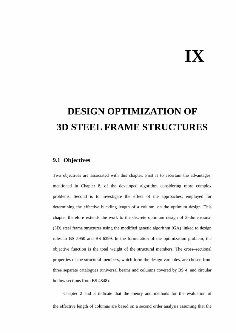
The local and global coordinate systems shown in Figure 9.1 are assumed in order to
correlate between the indices given by BS 5950 and that employed in the context. Figure
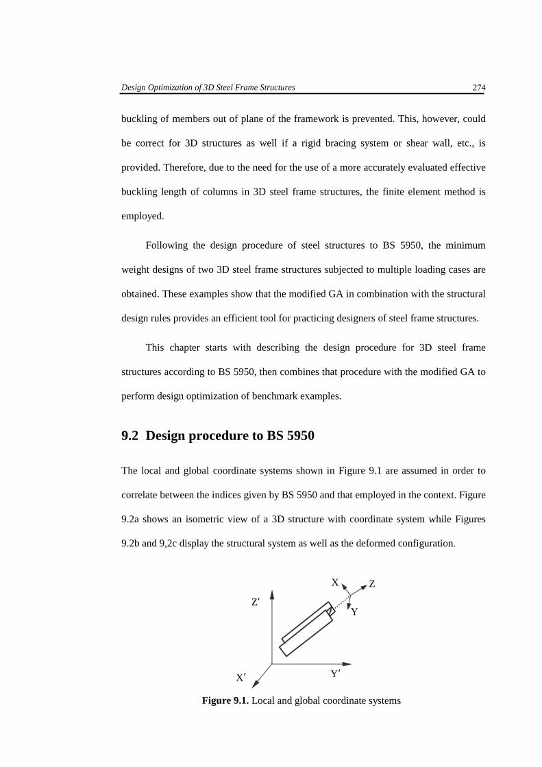
9.2a shows an isometric view of a 3D structure with coordinate system while Figures
9.2b and 9,2c display the structural system as well as the deformed configuration.
Figure 9.1. Local and global coordinate systems
Y ′
Z′
X ′
Z
Y
X
Design Optimization of 3D Steel Frame Structures
275
Lmemc,Y n′∆
Umemc,Y n′∆
Y ′
X X
X
X
Umemc,X n′∆
snh maxmemb
nδ
11x
,I
1sx
,nI
X Y
Y
Y
Y
Y
Y Y
Y
1bsx
+N,nI
X
X X
X
X
X
X
maxmemb
Nδ
Figure 9.2. 3D structure with the coordinate system and deformed configuration
1h
1B bNB
Z′
(b) YZ ′−′ projection of the 3D structure
snh Lmemc
X n,′∆ max
memb
nδ
X
Y
Y
Y
X
X X
1h
1SP bb
NSP
Z′
X ′
Y
X
Y
Y
X
Y
Y
Y
Y
1b1x
+N,I
2
Z′
Y ′ X ′
(a) Isometric view
Successive frameworks Transverse beams
Bracing system
(c) XZ ′−′ projection of the 3D structure
Design Optimization of 3D Steel Frame Structures
276
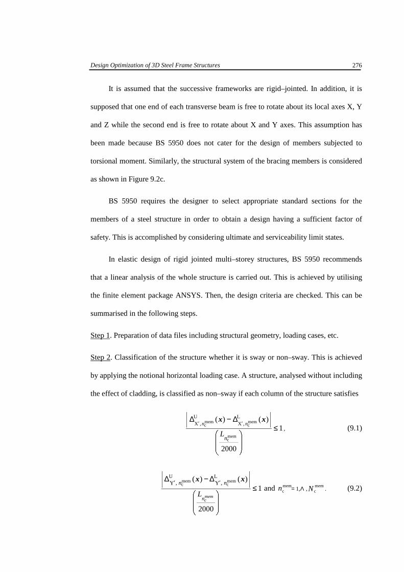
It is assumed that the successive frameworks are rigid–jointed. In addition, it is
supposed that one end of each transverse beam is free to rotate about its local axes X, Y
and Z while the second end is free to rotate about X and Y axes. This assumption has
been made because BS 5950 does not cater for the design of members subjected to
torsional moment. Similarly, the structural system of the bracing members is considered
as shown in Figure 9.2c.
BS 5950 requires the designer to select appropriate standard sections for the
members of a steel structure in order to obtain a design having a sufficient factor of
safety. This is accomplished by considering ultimate and serviceability limit states.
In elastic design of rigid jointed multi–storey structures, BS 5950 recommends
that a linear analysis of the whole structure is carried out. This is achieved by utilising
the finite element package ANSYS. Then, the design criteria are checked. This can be
summarised in the following steps.
Step 1. Preparation of data files including structural geometry, loading cases, etc.
Step 2. Classification of the structure whether it is sway or non–sway. This is achieved
by applying the notional horizontal loading case. A structure, analysed without including
the effect of cladding, is classified as non–sway if each column of the structure satisfies
1
2000
)()(
memc
memc
memc
LX
UX
≤��
�
�
��
�
�∆−∆
′′
nL
n,n,xx
, (9.1)
1
2000
)()( LUmemc
memc YY
≤��
�
�
�∆−∆ ′′
memcn
L
n,n,xx
and memc
memc 1 Nn ,,Λ= . (9.2)
Design Optimization of 3D Steel Frame Structures
277
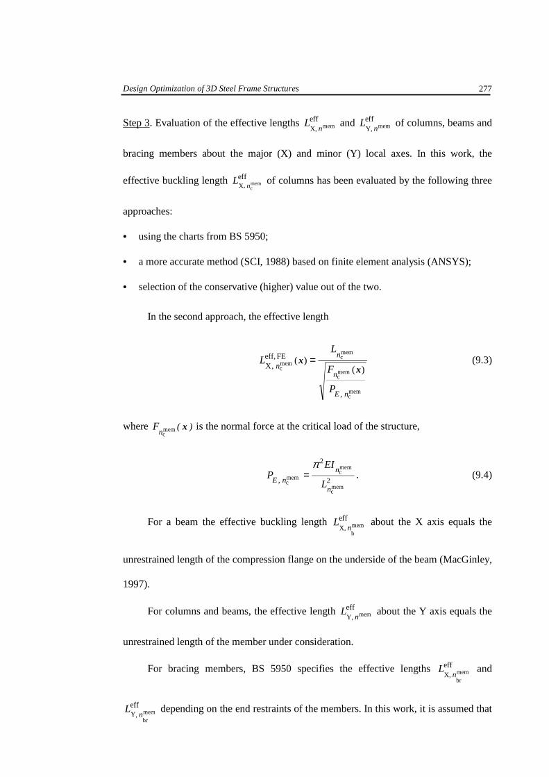
Step 3. Evaluation of the effective lengths effmemX, n
L and effmemY, n
L of columns, beams and
bracing members about the major (X) and minor (Y) local axes. In this work, the
effective buckling length effmemc,X n
L of columns has been evaluated by the following three
approaches:
• using the charts from BS 5950;
• a more accurate method (SCI, 1988) based on finite element analysis (ANSYS);
• selection of the conservative (higher) value out of the two.
In the second approach, the effective length
memc
memc
memc
memc )(
)(FE eff,X
n,E
n
n
n,
P
F
LL
xx = (9.3)
where )(n
F xmemc
is the normal force at the critical load of the structure,
2
2
memc
memc
memc
n
nn,E L
EIP
π= . (9.4)
For a beam the effective buckling length effmemb
X, nL about the X axis equals the
unrestrained length of the compression flange on the underside of the beam (MacGinley,
1997).
For columns and beams, the effective length effmemY, n
L about the Y axis equals the
unrestrained length of the member under consideration.
For bracing members, BS 5950 specifies the effective lengths effmembr
X, nL and
effmembr
,Y nL depending on the end restraints of the members. In this work, it is assumed that
Design Optimization of 3D Steel Frame Structures
278
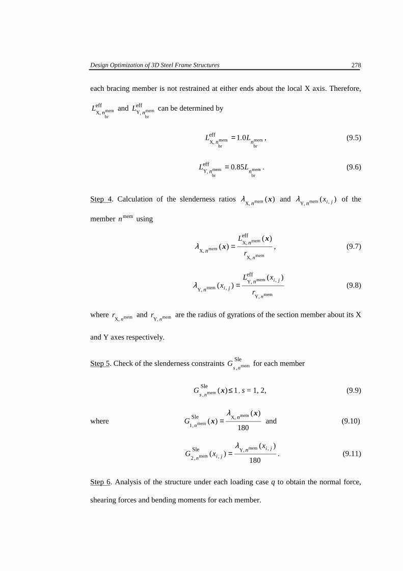
each bracing member is not restrained at either ends about the local X axis. Therefore,
effmembr
X, nL and eff
membr
,Y nL can be determined by
membr
membr
01effX, nn
L.L = , (9.5)
membr
membr
850eff,Y nn
L.L = . (9.6)
Step 4. Calculation of the slenderness ratios )(memX,x
nλ and )(memY, j,ix
nλ of the
member memn using
mem
mem
mem
X,
X,
X,
)()(
eff
nr
Ln
n
xx =λ , (9.7)
mem
mem
mem
Y,
Y,
Y,
)()(
eff
n
j,i
j,ir
xLx
n
n=λ (9.8)
where memX, nr and memY, n
r are the radius of gyrations of the section member about its X
and Y axes respectively.
Step 5. Check of the slenderness constraints Sle
memn,sG for each member
1)(Sle
mem ≤xn,s
G , s = 1, 2, (9.9)
where 180
)()(
mem
memX,
1
Slex
x n
n,G
λ= and (9.10)
180
)()(
mem
memY,
2
Sle j,i
j,in,
xxG
nλ
= . (9.11)
Step 6. Analysis of the structure under each loading case q to obtain the normal force,
shearing forces and bending moments for each member.

Design Optimization of 3D Steel Frame Structures
279
Step 7. Check of the strength criteria for each member memn under the loading case q as
follows:
a) Determination of the type of the section of the member (e.g. slender, semi–compact,
compact or plastic).
b) Evaluation of the design strength memy n,p of the member.
c) Check of the strength constraints )(Str
mem xq,
n,rG depending on whether the member is
in tension or compression. This stage contains five checks (r = 5) for each member
under each loading case q. The strength constraints are local capacity, overall
capacity, shear capacities in X and Y directions and the shear buckling capacity.
These can be expressed as follows:
1)(Str
mem ≤xq,
n,rG , r = 1, 2, 3, 4, 5 and q = 1,2, Q,Λ (9.12)
where the local capacity
��������
�
��������
�
�
++
++
=
members comprissonfor)(
)(
)(
)(
)()(
)(
(9.13)
memberstensionfor)(
)(
)(
)(
)()(
)(
)(
mem
mem
mem
mem
memmem
mem
mem
mem
mem
mem
memmem
mem
mem
CY
Y,
CX
X,
yg,
CY
Y,
CX
X,
ye,
1
Str
j,i
j,ij,ij,i
j,i
j,ij,ij,i
q,
xM
M
xM
M
xpxA
F
xM
M
xM
M
xpxA
F
G
n,
q
n
n,
q
n
n,n
q
n
n,
q
n
n,
q
n
n,n
q
n
n,
x
xx
x
xx
x
where )(mem xq
nF is the axial force. The applied moment about the local axes X and Y
are )(memX,xq
nM and )(memY,
xq
nM . The design strength is )(memy, j,ixp
n. The moment
Design Optimization of 3D Steel Frame Structures
280
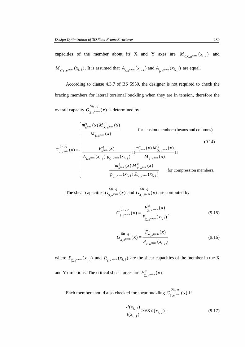
capacities of the member about its X and Y axes are )(memCX j,in,xM and
)(memCY j,in,xM . It is assumed that )(and)( memmem g,e, j,ij,i xAxA
nn are equal.
According to clause 4.3.7 of BS 5950, the designer is not required to check the
bracing members for lateral torsional buckling when they are in tension, therefore the
overall capacity )(Str
mem2x
q,
n,G is determined by
������
�
������
�
�
++=
members.n compressiofor)()(
)()(
)(
)()(
)()(
)(
(9.14)
columns)and(beams memberstensionfor)(
)()(
)(
memmem
memmem
mem
memmem
memmem
mem
mem
memmem
mem
Yy
Y,
b
X,
Cg,
b
X,
2
Str
j,ij,i
j,i
q,
xZxp
Mm
M
Mm
xpxA
F
M
Mm
G
n,n,
q
n
q
n
n,
q
n
q
n
n,j,in
q
n
n,
q
n
q
n
n,
xx
x
xxx
x
xx
x
The shear capacities )(Str
mem3x
q,
n,G and )(
Strmem4
xq,
n,G are computed by
)(
)()(
mem
mem
mem
X,
X,
3
Str
j,in
q
n
n, xP
FG
q, xx = , (9.15)
)(
)()(
mem
mem
mem
Y,
Y,
4
Str
j,in
q
n
n, xP
FG
q, xx = (9.16)
where )(memX, j,inxP and )(memY, j,in
xP are the shear capacities of the member in the X
and Y directions. The critical shear forces are )(memX,xq
nF .
Each member should also checked for shear buckling )(Str
mem5x
q,
n,G if
)(63)(
)(,
,
,ji
ji
jix
xt
xdε≥ . (9.17)
Design Optimization of 3D Steel Frame Structures
281
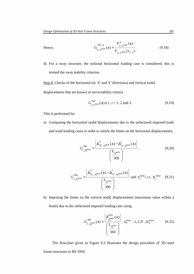
Hence, )(
)()(
mem
mem
mem
cr,
Y,
4
Str
j,in
q
n
n, xV
FG
q, xx = . (9.18)
d) For a sway structure, the notional horizontal loading case is considered, this is
termed the sway stability criterion.
Step 8. Checks of the horizontal (in YandX ′′ directions) and vertical nodal
displacements that are known as serviceability criteria
1)(Ser
mem ≤xn,t
G , t = 1, 2 and 3. (9.19)
This is performed by:
a) Computing the horizontal nodal displacements due to the unfactored imposed loads
and wind loading cases in order to satisfy the limits on the horizontal displacements,
��
�
�
�∆−∆
=′′
300
)()(
memc
memc
U
memc
memc
L
X
1
XSer
n
n,
n LG
n,
,
xx, (9.20)
��
�
�
�∆−∆
=′′
300
)()(
memc
L
memc
U
memc
memc
YYSer
2n
, LG
n,n,
n
xx and mem
cmemc 1 Nn ,,Λ= . (9.21)
b) Imposing the limits on the vertical nodal displacements (maximum value within a
beam) due to the unfactored imposed loading case using
��
�
�
�=
360
)()(
memb
memb
memb
max
2
Ser
n
n
n, LG
xx
δ, mem
bmemb 21 N,,,n Λ= . (9.22)
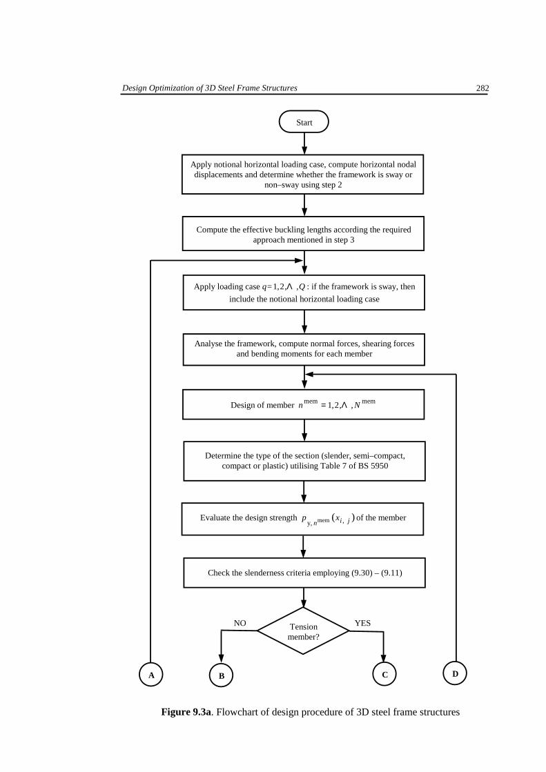
The flowchart given in Figure 9.3 illustrates the design procedure of 3D steel
frame structures to BS 5950.
Design Optimization of 3D Steel Frame Structures
282
YES NO
Start
Apply notional horizontal loading case, compute horizontal nodal displacements and determine whether the framework is sway or
non–sway using step 2
Apply loading case q= Q,,, Λ21 : if the framework is sway, then
include the notional horizontal loading case
Analyse the framework, compute normal forces, shearing forces and bending moments for each member
Design of member memn mem21 N,,, Λ=
Evaluate the design strength )(memy, j,inxp of the member
Tension member?
Compute the effective buckling lengths according the required approach mentioned in step 3
Determine the type of the section (slender, semi–compact, compact or plastic) utilising Table 7 of BS 5950
Figure 9.3a. Flowchart of design procedure of 3D steel frame structures
Check the slenderness criteria employing (9.30) – (9.11)
D C B A
Design Optimization of 3D Steel Frame Structures
283
NO
YES
NO
YES
B
Local capacity check Local capacity check
Lateral torsional buckling check Overall capacity check
Check of the serviceability criteria using (9.19) – (9.22)
Is memn = memN ?
Is q = Q?
Compute the horizontal and vertical nodal displacements due to the specified loading cases
Carry out the checks of shear applying (9.15) − (9.16) and shear buckling using (9.18) if necessary
C
End
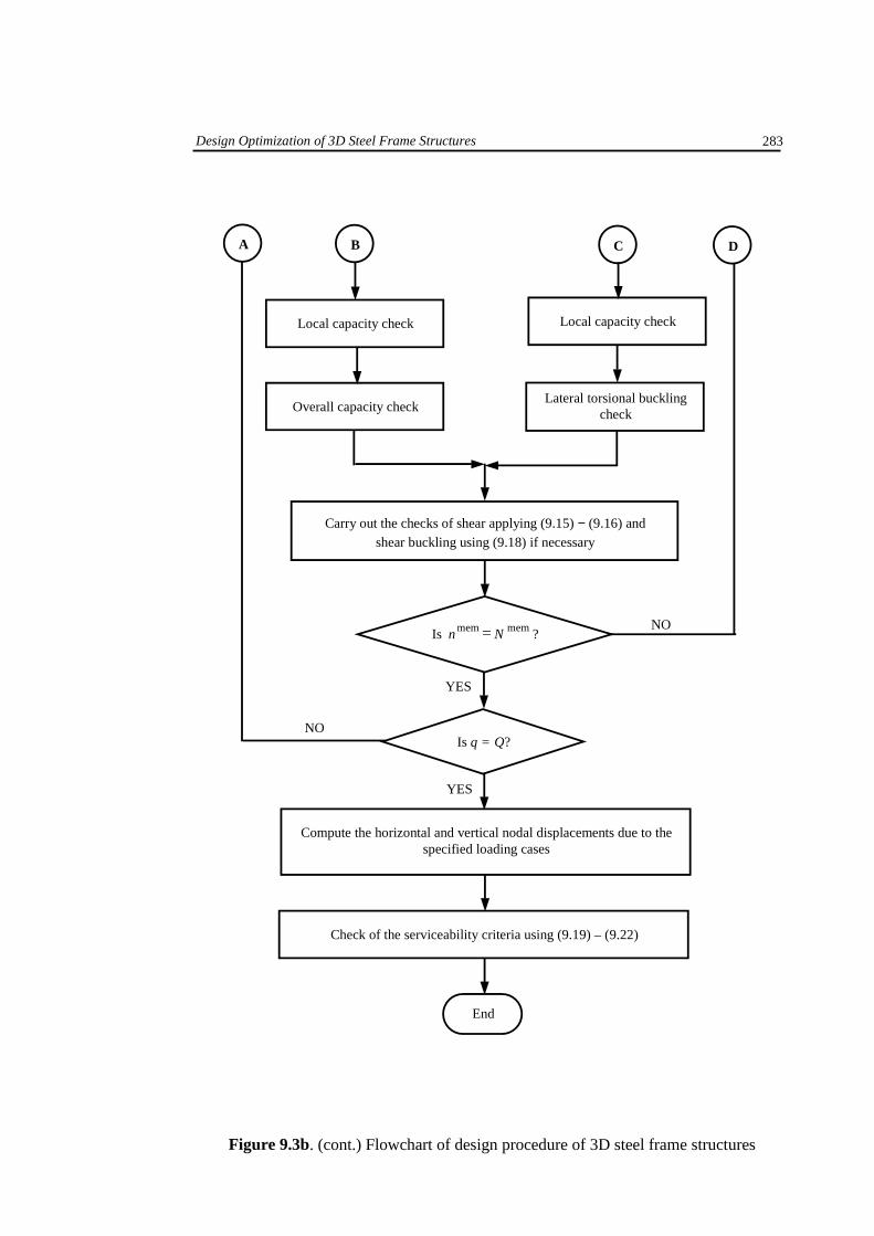
Figure 9.3b. (cont.) Flowchart of design procedure of 3D steel frame structures
D A
Design Optimization of 3D Steel Frame Structures
284
9.3 Problem formulation and solution technique
The general formulation of the design optimization problem can be expressed by
�
=
=mem
memmemmem
1
)(MinimizeN
nnn
LWF x
subject to: 1)(Str
mem ≤xq,
n,rG , r = 1, 2, 3, 4, q = 1, 2, Q,Λ
1)(Sle
mem ≤xn,s
G , s = 1, 2
1)(Ser
mem ≤xn,t
G , t = 1, 2, 3
1bs
bs
1x
x ≤− n,n
n,n
I
I, ss 21 N,,,n Λ= , 121 bb += N,,,n Λ (9.23)
)21( TTTTJj ,,,, xxxxx Λ= , J,,,j Λ21=
jji Dx ∈, and
)(21 λ
Λ,j
,,,j
,,jj dddD =
where memnW is the mass per unit length of the member under consideration and is taken
from a catalogue. The strength, slenderness and serviceability criteria are )(Str
mem xq,
n,rG ,
)(Sle
mem xn,s
G and )(Ser
mem xn,t
G respectively. The vector of design variables x is divided
into J sub–vectors Jx . The components of these sub–vectors take values from a
corresponding catalogue jD . In the present work, the cross–sectional properties of the
structural members, which form the design variables, are chosen from three separate
catalogues (universal beams and columns covered by BS 4, and circular hollow sections
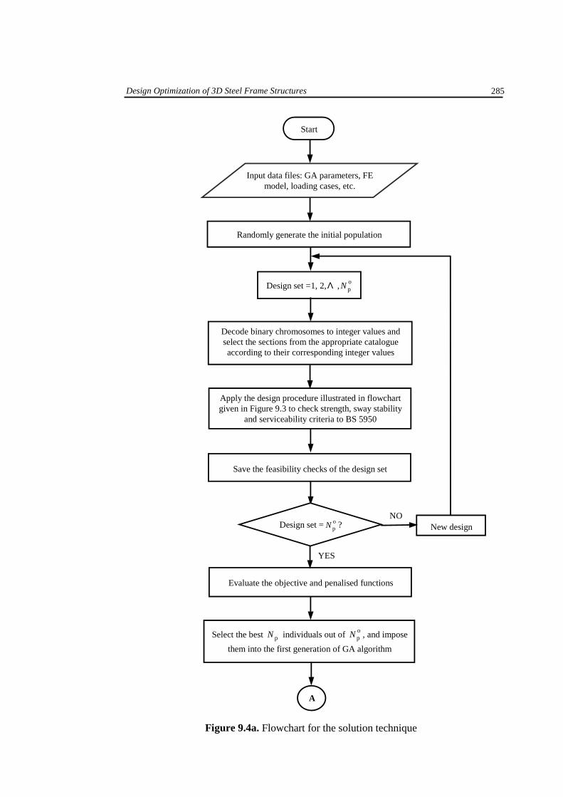
from BS 4848). Figure 9.4 demonstrates the applied solution technique.
Design Optimization of 3D Steel Frame Structures
285
YES
NO
Save the feasibility checks of the design set
Randomly generate the initial population
Design set =1, 2, opN,Λ
Evaluate the objective and penalised functions
Select the best pN individuals out of opN , and impose
them into the first generation of GA algorithm
New design
Apply the design procedure illustrated in flowchart given in Figure 9.3 to check strength, sway stability
and serviceability criteria to BS 5950
A
Start
Decode binary chromosomes to integer values and select the sections from the appropriate catalogue according to their corresponding integer values
Figure 9.4a. Flowchart for the solution technique
Input data files: GA parameters, FE model, loading cases, etc.
Design set = opN ?
YES
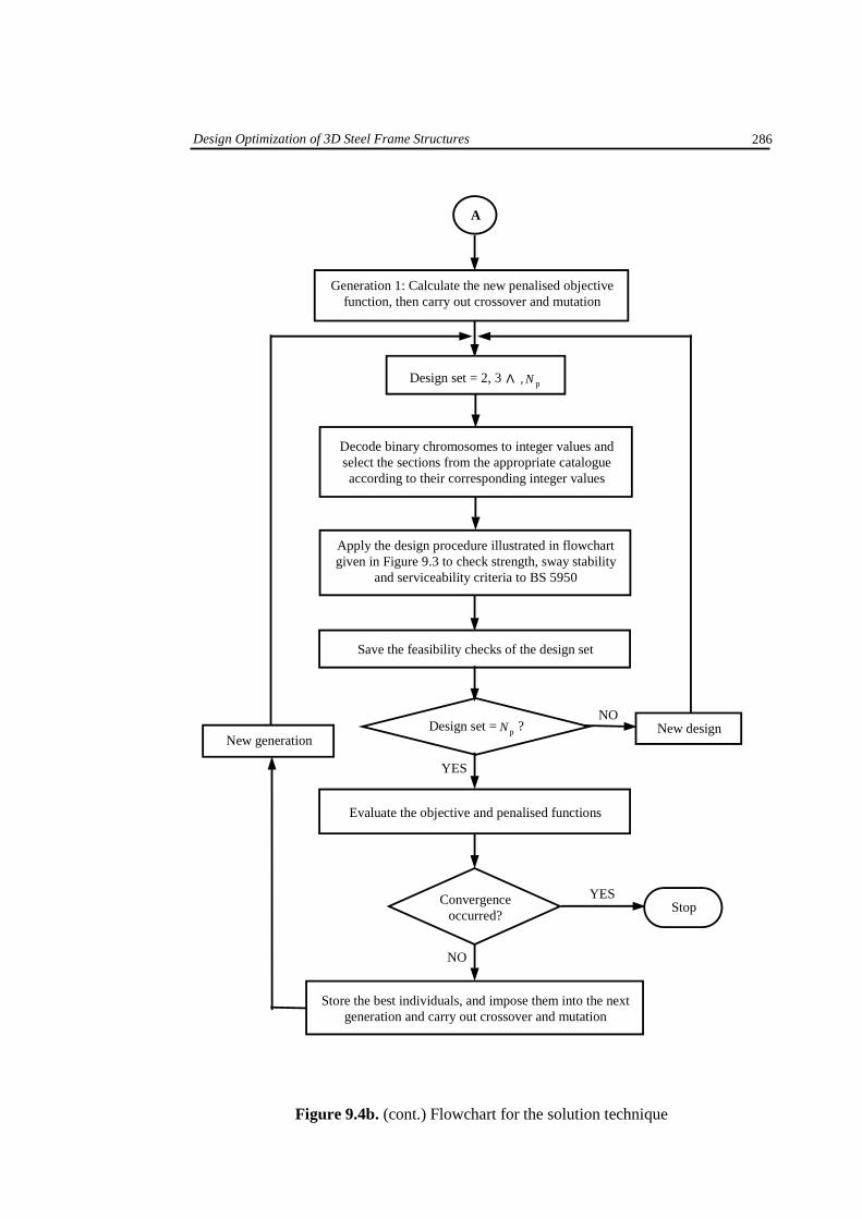
Design Optimization of 3D Steel Frame Structures
286
YES
YES
NO
NO
Save the feasibility checks of the design set
Generation 1: Calculate the new penalised objective function, then carry out crossover and mutation
Design set = pN ?
Convergence occurred?
A
Stop
Store the best individuals, and impose them into the next generation and carry out crossover and mutation
Figure 9.4b. (cont.) Flowchart for the solution technique
New generation New design
Design set = 2, 3 pN,Λ
Decode binary chromosomes to integer values and select the sections from the appropriate catalogue according to their corresponding integer values
Apply the design procedure illustrated in flowchart given in Figure 9.3 to check strength, sway stability
and serviceability criteria to BS 5950
Evaluate the objective and penalised functions
Design Optimization of 3D Steel Frame Structures
287
9.4 Benchmark examples
Having introduced the design procedure according to BS 5950 linked to the GA
procedure and the formulation of design optimization problem, the process of
optimization in now carried out.
Two steel frame structures are demonstrated here to illustrate the effectiveness and
benefits of the developed GA technique as well as investigating the effect of the
employed approach for the determination of the effective buckling length on the
optimum design attained.
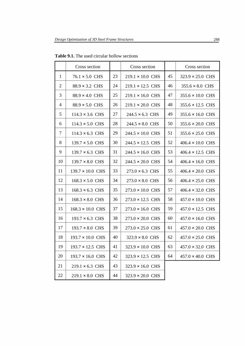
The catalogue of available cross sections in BS 4 include 64 universal beams (UB)
and 32 universal columns (UC). These sections are given in Section 7.2.1. The
catalogue of circular hollow sections (CHS) is taken from BS 4848 and this includes 64
sections, listed in Table 9.1, varying from 76.1 × 5.0 CHS to 457.0 × 40.0 CHS.
In the present work, the initial population size opN is assumed to be 1000 and
fixed population size pN of 70 during successive generations, elite percentage rE was
30 %, probability of crossover cP was 0.7, probability of mutation mP was 0.01 and
one–point crossover is applied. In addition, the technique described in Section 6.2 is
utilised where the simple "exact" penalty function employed is
Minimize �� �=
violated.sconstraintofany0
satisfiedsconstraintall)(C)(
,
,F-F
xx (9.24)
The convergence criteria and termination conditions detailed in Section 5.6.3.7 are
used where avC = 0.001, cuC = 0.001 and 200max =gen .
Design Optimization of 3D Steel Frame Structures
288
Table 9.1. The used circular hollow sections
Cross section Cross section Cross section
1 76.1 × 5.0 CHS 23 219.1 × 10.0 CHS 45 323.9 × 25.0 CHS
2 88.9 × 3.2 CHS 24 219.1 × 12.5 CHS 46 355.6 × 8.0 CHS
3 88.9 × 4.0 CHS 25 219.1 × 16.0 CHS 47 355.6 × 10.0 CHS
4 88.9 × 5.0 CHS 26 219.1 × 20.0 CHS 48 355.6 × 12.5 CHS
5 114.3 × 3.6 CHS 27 244.5 × 6.3 CHS 49 355.6 × 16.0 CHS
6 114.3 × 5.0 CHS 28 244.5 × 8.0 CHS 50 355.6 × 20.0 CHS
7 114.3 × 6.3 CHS 29 244.5 × 10.0 CHS 51 355.6 × 25.0 CHS
8 139.7 × 5.0 CHS 30 244.5 × 12.5 CHS 52 406.4 × 10.0 CHS
9 139.7 × 6.3 CHS 31 244.5 × 16.0 CHS 53 406.4 × 12.5 CHS
10 139.7 × 8.0 CHS 32 244.5 × 20.0 CHS 54 406.4 × 16.0 CHS
11 139.7 × 10.0 CHS 33 273.0 × 6.3 CHS 55 406.4 × 20.0 CHS
12 168.3 × 5.0 CHS 34 273.0 × 8.0 CHS 56 406.4 × 25.0 CHS
13 168.3 × 6.3 CHS 35 273.0 × 10.0 CHS 57 406.4 × 32.0 CHS
14 168.3 × 8.0 CHS 36 273.0 × 12.5 CHS 58 457.0 × 10.0 CHS
15 168.3 × 10.0 CHS 37 273.0 × 16.0 CHS 59 457.0 × 12.5 CHS
16 193.7 × 6.3 CHS 38 273.0 × 20.0 CHS 60 457.0 × 16.0 CHS
17 193.7 × 8.0 CHS 39 273.0 × 25.0 CHS 61 457.0 × 20.0 CHS
18 193.7 × 10.0 CHS 40 323.9 × 8.0 CHS 62 457.0 × 25.0 CHS
19 193.7 × 12.5 CHS 41 323.9 × 10.0 CHS 63 457.0 × 32.0 CHS
20 193.7 × 16.0 CHS 42 323.9 × 12.5 CHS 64 457.0 × 40.0 CHS
21 219.1 × 6.3 CHS 43 323.9 × 16.0 CHS
22 219.1 × 8.0 CHS 44 323.9 × 20.0 CHS
Design Optimization of 3D Steel Frame Structures
289
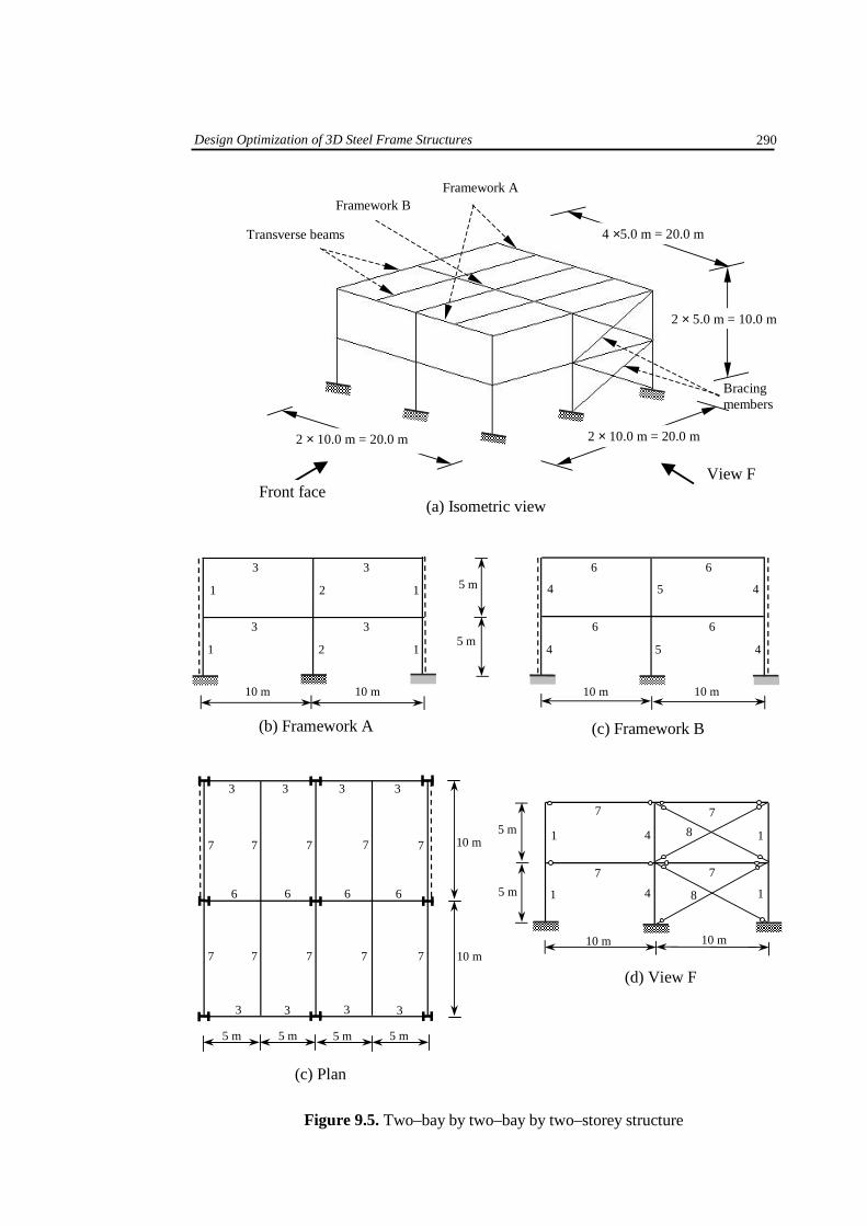
9.4.1 Example 1: Two–bay by two–bay by two–storey structure
The first 3D steel frame structure, analysed in this chapter, is the two–bay by two–bay
by two–storey structure shown in Figure 9.5. It can be observed from Figure 9.5a that
the structure consists of three successive frameworks, transverse beams and the bracing
system. The spacing between the successive frameworks is 10.0 m while the distance
between the successive transverse beams is 5 m.
Because BS 5950 does not cater for the design of members subjected to torsional
moments, it is assumed that one end of each transverse beam is free to rotate about its
local axes X, Y and Z while the second end is free to rotate about X and Y axes.
Similarly, the structural system of the bracing members is considered. The structural
system is shown in Figures 9.5b–9.5d.
The structure was designed for use as an office block including projection rooms.
Nine loading cases were taken into account and these represent the most unfavourable
combinations of the factored dead load (DL), imposed load (LL) and wind load (WL) as
required by BS 5950 and BS 6399. Because the structure is doubly–symmetric, two
orthogonal wind cases have been considered where the wind loads are factored by 1.2.
The values of the unfactored DL and LL are tabulated in Table 9.2. These values are
calculated according to the recommendations given by Owens et al (1992), MacGinley
(1997) and Nethercot (1995).
Table 9.2. The values of dead load and imposed load
Value of the load on roof
Value of the load on first floor
DL 7.0 kN/m2 9.0 kN/m2
LL 2.0 kN/m2 5.0 kN/m2
Design Optimization of 3D Steel Frame Structures
290
Bracing members
Framework B
Transverse beams
2 × 10.0 m = 20.0 m 2 × 10.0 m = 20.0 m
4 ×5.0 m = 20.0 m
View F
(a) Isometric view
10 m 10 m 10 m 10 m
5 m
5 m 1
1 1
1
4
4
4
4
3 3 6 6
6 6 3 3
5
5
2
2
(b) Framework A (c) Framework B
5 m 5 m 5 m 5 m
7 7
10 m 10 m
5 m
5 m
10 m
10 m
3 3
7 7
7 7
8
8
3 3
3 3 3 3
6 6 6 6
1
1
1
1 4
4
(d) View F 7 7
7 7 7
7 7 7
(c) Plan
Framework A
Figure 9.5. Two–bay by two–bay by two–storey structure
2 × 5.0 m = 10.0 m
Front face
Design Optimization of 3D Steel Frame Structures
291
The reinforced concrete slabs are assumed to transmit the loads in one direction
because the ratio of the spacing between the successive frameworks and the distances
between the successive transverse beams equal 2 (see MacGinley, 1997).
According to BS 6399: Part 2, the standard method was utilised to determine the
values of the wind pressures on the vertical walls and the flat roof assuming
1. the openings are dominant,
2. the building type factor equal 4.0,
3. the reference height of the structure (Hr) equal to the maximum height of the
structure above the ground level (10.0 m),
4. the basic wind speed bV is 23 m/s,
5. the terrain and building factor bS is 1.58,
6. the altitude factor aS , the directional factor dS , the seasonal factor sS and the
probability factor pS equal 1.0,
7. the size effect factor aC is taken as 0.90,
8. the external pressure coefficient peC for each surface of the building is determined
according table 5 and 8 of BS 6399 and
9. the internal pressure coefficient piC for each surface of the structure is
pepi 750 C.C = (9.25)
where peC is the external pressure coefficient of the surface under consideration.
At this stage having introduced the basic assumptions for evaluating the design
loads, the values of these loads can accordingly be computed depending on the nine
loading cases summarised bellow:
1. the floors are subjected to the vertical uniform loads LL.DL.P 6141v += ,
Design Optimization of 3D Steel Frame Structures
292
2. the floors are subjected to the vertical uniform loads LL.DL.P 6141v += , and left
hand side (LHS) nodes of each framework are subjected to the horizontal
concentrated loads due to the notional horizontal loading condition,
3. the floors of the first bay (counting from the left) are subjected to the vertical
uniform loads DL.P 41v = while the rest of the floors are subjected to
LL.DL.P 6141v += ,
4. the floors are subjected to a staggered arrangement of vertical uniform loads
LL.DL.P 6141v += and DL.P 41v = ,
5. the floors are subjected to the vertical uniform loads LL.DL.P 2121v += and the
structure is subjected to the first factored wind loading case when the LHS face of
the structure is the windward face,
6. the floors are subjected to the vertical uniform loads LL.DL.P 2121v += and the
structure is subjected to the second factored wind loading case when the front face
of the structure is the windward face,
7. the floors are subjected to the vertical uniform load LLP .01v = ,
8. the floors are subjected to the vertical uniform loads LLP .01v = and the structure is
subjected to the first unfactored wind loading case when the LHS face of the
structure is the windward face and
9. the floors are subjected to the vertical uniform loads LLP .01v = and the structure is
subjected to the second unfactored wind loading case when the front face of the
structure is the windward face.
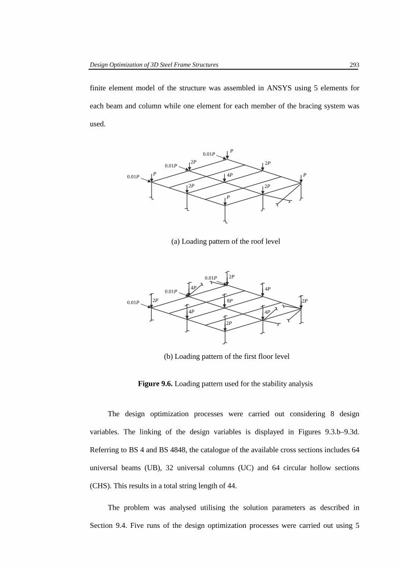
A more accurately evaluated effective buckling length of columns was determined
using the finite element method using the loading pattern displayed in Figure 9.6. The
Design Optimization of 3D Steel Frame Structures
293
finite element model of the structure was assembled in ANSYS using 5 elements for
each beam and column while one element for each member of the bracing system was
used.
The design optimization processes were carried out considering 8 design
variables. The linking of the design variables is displayed in Figures 9.3.b–9.3d.
Referring to BS 4 and BS 4848, the catalogue of the available cross sections includes 64
universal beams (UB), 32 universal columns (UC) and 64 circular hollow sections
(CHS). This results in a total string length of 44.
The problem was analysed utilising the solution parameters as described in
Section 9.4. Five runs of the design optimization processes were carried out using 5
0.01P
0.01P
0.01P
P 4P P
2P
P
2P
2P 2P
P
0.01P
0.01P
0.01P
2P 8P 2P
4P
2P
4P
4P 4P
2P
(a) Loading pattern of the roof level
(b) Loading pattern of the first floor level
Figure 9.6. Loading pattern used for the stability analysis
Design Optimization of 3D Steel Frame Structures
294
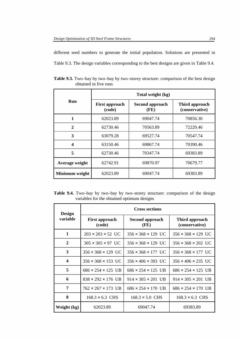
different seed numbers to generate the initial population. Solutions are presented in
Table 9.3. The design variables corresponding to the best designs are given in Table 9.4.
Table 9.3. Two–bay by two–bay by two–storey structure: comparison of the best design obtained in five runs
Total weight (kg)
Run First approach
(code) Second approach
(FE) Third approach (conservative)
1 62023.89 69047.74 70856.30
2 62730.46 70563.89 72220.46
3 63079.28 69527.74 70547.74
4 63150.46 69867.74 70390.46
5 62730.46 70347.74 69383.89
Average weight 62742.91 69870.97 70679.77
Minimum weight 62023.89 69047.74 69383.89
Table 9.4. Two–bay by two–bay by two–storey structure: comparison of the design variables for the obtained optimum designs
Cross sections Design
var iable First approach (code)
Second approach (FE)
Third approach (conservative)
1 203 × 203 × 52 UC 356 × 368 × 129 UC 356 × 368 × 129 UC
2 305 × 305 × 97 UC 356 × 368 × 129 UC 356 × 368 × 202 UC
3 356 × 368 × 129 UC 356 × 368 × 177 UC 356 × 368 × 177 UC
4 356 × 368 × 153 UC 356 × 406 × 393 UC 356 × 406 × 235 UC
5 686 × 254 × 125 UB 686 × 254 × 125 UB 686 × 254 × 125 UB
6 838 × 292 × 176 UB 914 × 305 × 201 UB 914 × 305 × 201 UB
7 762 × 267 × 173 UB 686 × 254 × 170 UB 686 × 254 × 170 UB
8 168.3 × 6.3 CHS 168.3 × 5.0 CHS 168.3 × 6.3 CHS
Weight (kg) 62023.89 69047.74 69383.89
Design Optimization of 3D Steel Frame Structures
295
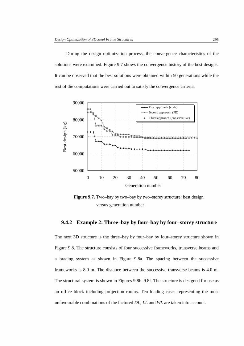
During the design optimization process, the convergence characteristics of the
solutions were examined. Figure 9.7 shows the convergence history of the best designs.
It can be observed that the best solutions were obtained within 50 generations while the
rest of the computations were carried out to satisfy the convergence criteria.
Figure 9.7. Two–bay by two–bay by two–storey structure: best design
versus generation number
9.4.2 Example 2: Three–bay by four–bay by four–storey structure
The next 3D structure is the three–bay by four–bay by four–storey structure shown in
Figure 9.8. The structure consists of four successive frameworks, transverse beams and
a bracing system as shown in Figure 9.8a. The spacing between the successive
frameworks is 8.0 m. The distance between the successive transverse beams is 4.0 m.
The structural system is shown in Figures 9.8b–9.8f. The structure is designed for use as
an office block including projection rooms. Ten loading cases representing the most
unfavourable combinations of the factored DL, LL and WL are taken into account.
Generation number
50000
60000
70000
80000
90000
0 10 20 30 40 50 60 70 80
First approach (code)
Second approach (FE)
Third approach (conservative)
Bes
t des
ign
(kg)

Design Optimization of 3D Steel Frame Structures
296
Figure 9.8. Three–bay by four–bay by four–storey structure
(a) Isometric view
Framework A
Framework D
Framework B
Framework C
Transverse beams
View F
Bracing system
6 × 4.0 m = 24.0 m
17.0 m
4 × 8.0 m = 32.0 m
Front face
12
12
(d) Framework C
11 11
4 m 7
7
1
1
2 2
2
2
5
2
2 2
2
8 m 8 m 8 m 8 m
4 m
5
12
11 11 11 11
11 11 12
12
12 11
4 m
5 m
8 m
7
7
10
7
7
8 m
10
11 11
7
7
11 1
1
2
6
6
(e) Framework D (f) View F
2
4 m
4 m
4 m
5 m
(b) Framework A
5 5 5
5 5 5
2 2 4 4
2
3 1
1
4 2 4
1
1 3 3
3
5 5 5
5 5 5
8 m 8 m 8 m
(c) Framework B
10 10
10 10 10
10
9 7 9 7
8 m 8 m 8 m
6
6
6
6 8 10 10 10
8
8
8
7 7 9 9
10 10 10
Design Optimization of 3D Steel Frame Structures
297
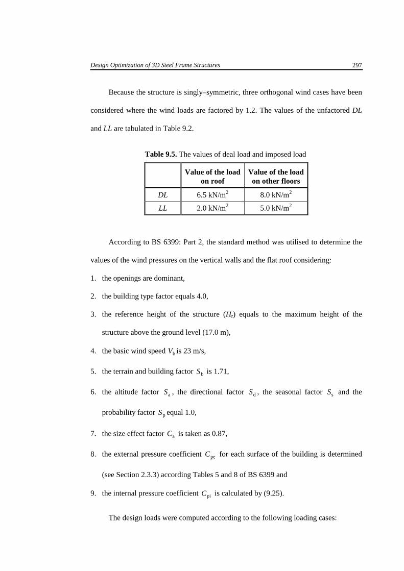
Because the structure is singly–symmetric, three orthogonal wind cases have been
considered where the wind loads are factored by 1.2. The values of the unfactored DL
and LL are tabulated in Table 9.2.
Table 9.5. The values of deal load and imposed load
Value of the load on roof
Value of the load on other floors
DL 6.5 kN/m2 8.0 kN/m2
LL 2.0 kN/m2 5.0 kN/m2
According to BS 6399: Part 2, the standard method was utilised to determine the
values of the wind pressures on the vertical walls and the flat roof considering:
1. the openings are dominant,
2. the building type factor equals 4.0,
3. the reference height of the structure (Hr) equals to the maximum height of the
structure above the ground level (17.0 m),
4. the basic wind speed bV is 23 m/s,
5. the terrain and building factor bS is 1.71,
6. the altitude factor aS , the directional factor dS , the seasonal factor sS and the
probability factor pS equal 1.0,
7. the size effect factor aC is taken as 0.87,
8. the external pressure coefficient peC for each surface of the building is determined
(see Section 2.3.3) according Tables 5 and 8 of BS 6399 and
9. the internal pressure coefficient piC is calculated by (9.25).
The design loads were computed according to the following loading cases:
Design Optimization of 3D Steel Frame Structures
298
1. the floors are subjected to the vertical uniform loads LL.DL.P 6141v += ,
2. the floors are subjected to the vertical uniform loads LL.DL.P 6141v += , and left
hand side (LHS) nodes of each framework are subjected to the horizontal
concentrated loads due to the notional horizontal loading condition (see Chapter 2),
3. the floors of the first bay (counting from the left) are subjected to the vertical
uniform loads DL.P 41v = while the rest of the floors are subjected to
LL.DL.P 6141v += ,
4. the floors are subjected to a staggered arrangement of vertical uniform loads
LL.DL.P 6141v += and DL.P 41v = ,
5. the floors are subjected to the vertical uniform loads LL.DL.P 2121v += and the
structure is subjected to the first factored wind loading case when the LHS face of
the structure is the windward face,
6. the floors are subjected to the vertical uniform loads LL.DL.P 2121v += and the
structure is subjected to the second factored wind loading case when the front face
of the structure is the windward face,
7. the floors are subjected to the vertical uniform loads LL.DL.P 2121v += and the
structure is subjected to the third factored wind loading case when the rear face of
the structure is the windward face,
8. the floors are subjected to the vertical uniform load LLP 1.0v = ,
9. the floors are subjected to the vertical uniform loads LLP 1.0v = and the structure is
subjected to the first unfactored wind loading case when the LHS face of the
structure is the windward face and
Design Optimization of 3D Steel Frame Structures
299
10. the floors are subjected to the vertical uniform loads LLP 1.0v = and the structure is
subjected to the second unfactored wind loading case when the front face of the
structure is the windward face.
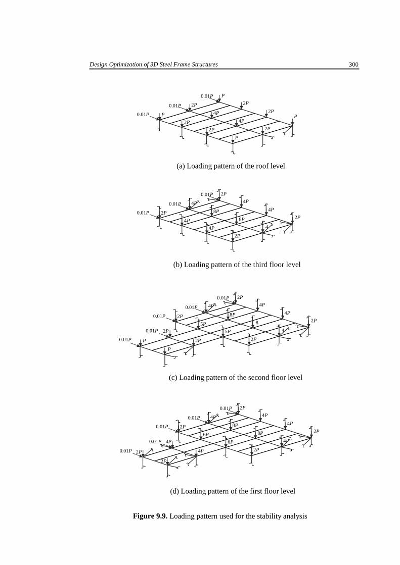
The finite element method was employed (see Toropov et al., 1999) in order to
evaluate the effective buckling length of columns. This was performed by utilising the
loading pattern displayed in Figure 9.9. In the finite element model, the structure was
assembled in ANSYS using 5 elements for each beam and column while one element
for each member of the bracing system.
The optimization process was carried out considering 12 design variables. The linking
of the design variables is displayed in Figures 9.8.b–9.8f.
Referring to BS 4 and BS 4848, the catalogue of the available cross sections
include 64 universal beams (UB), 32 universal columns (UC) and 64 circular hollow
sections (CHS). This results in a total string length of 64.
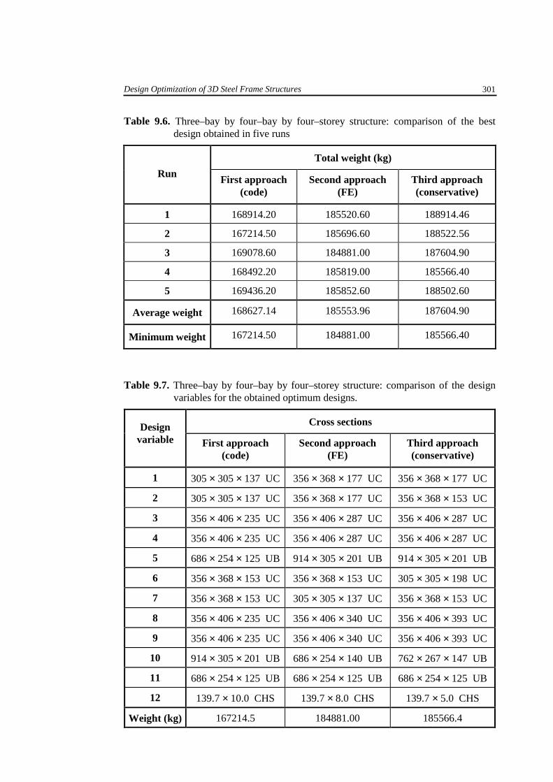
The problem was analysed utilising the solution parameters described in Section
9.4. Five runs of the optimization process were carried out using 5 different seed
numbers to generate the initial population. The optimization process was terminated
when any of the convergence criteria is satisfied. Solutions are presented in Table 9.6.
The design variables corresponding to the best designs are given in Table 9.7.
Design Optimization of 3D Steel Frame Structures
300
2P
4P 0.01P
0.01P
0.01P
P 4P
P
2P
P
2P
2P 2P
P
(a) Loading pattern of the roof level
(b) Loading pattern of the third floor level
Figure 9.9. Loading pattern used for the stability analysis
2P
4P
8P 0.01P
0.01P
0.01P
2P 8P 2P
4P
2P
4P
44P
2P
4P
(c) Loading pattern of the second floor level
P
2P
5P
8P 0.01P
0.01P
0.01P
2P 82P
4P
2P
4P
45P
2P
4P
2P
P
2P
4P
6P
8P 0.01P
0.01P
0.01P
2P 8P 2P
4P
2P
4P
4P 6P
2P
4P
4P
2P
(d) Loading pattern of the first floor level
0.01P
0.01P
0.01P
0.01P
Design Optimization of 3D Steel Frame Structures
301
Table 9.6. Three–bay by four–bay by four–storey structure: comparison of the best design obtained in five runs
Total weight (kg)
Run First approach (code)
Second approach (FE)
Third approach (conservative)
1 168914.20 185520.60 188914.46
2 167214.50 185696.60 188522.56
3 169078.60 184881.00 187604.90
4 168492.20 185819.00 185566.40
5 169436.20 185852.60 188502.60
Average weight 168627.14 185553.96 187604.90
Minimum weight 167214.50 184881.00 185566.40
Table 9.7. Three–bay by four–bay by four–storey structure: comparison of the design variables for the obtained optimum designs.
Cross sections Design var iable First approach
(code) Second approach
(FE) Third approach (conservative)
1 305 × 305 × 137 UC 356 × 368 × 177 UC 356 × 368 × 177 UC
2 305 × 305 × 137 UC 356 × 368 × 177 UC 356 × 368 × 153 UC
3 356 × 406 × 235 UC 356 × 406 × 287 UC 356 × 406 × 287 UC
4 356 × 406 × 235 UC 356 × 406 × 287 UC 356 × 406 × 287 UC
5 686 × 254 × 125 UB 914 × 305 × 201 UB 914 × 305 × 201 UB
6 356 × 368 × 153 UC 356 × 368 × 153 UC 305 × 305 × 198 UC
7 356 × 368 × 153 UC 305 × 305 × 137 UC 356 × 368 × 153 UC
8 356 × 406 × 235 UC 356 × 406 × 340 UC 356 × 406 × 393 UC
9 356 × 406 × 235 UC 356 × 406 × 340 UC 356 × 406 × 393 UC
10 914 × 305 × 201 UB 686 × 254 × 140 UB 762 × 267 × 147 UB
11 686 × 254 × 125 UB 686 × 254 × 125 UB 686 × 254 × 125 UB
12 139.7 × 10.0 CHS 139.7 × 8.0 CHS 139.7 × 5.0 CHS
Weight (kg) 167214.5 184881.00 185566.4
Design Optimization of 3D Steel Frame Structures
302
From Table 9.6, it can deduced that the optimizer was able to obtain several
solutions and the differences between them are small.
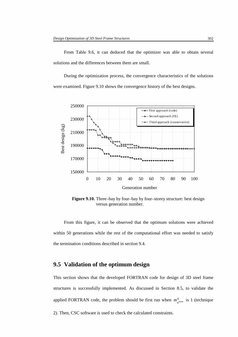
During the optimization process, the convergence characteristics of the solutions
were examined. Figure 9.10 shows the convergence history of the best designs.
Figure 9.10. Three–bay by four–bay by four–storey structure: best design versus generation number.
From this figure, it can be observed that the optimum solutions were achieved
within 50 generations while the rest of the computational effort was needed to satisfy
the termination conditions described in section 9.4.
9.5 Validation of the optimum design
This section shows that the developed FORTRAN code for design of 3D steel frame
structures is successfully implemented. As discussed in Section 8.5, to validate the
applied FORTRAN code, the problem should be first run when q
nm mem is 1 (technique
2). Then, CSC software is used to check the calculated constraints.
Bes
t des
ign
(kg)
Generation number
150000
170000
190000
210000
230000
250000
0 10 20 30 40 50 60 70 80 90 100
First approach (code)
Second approach (FE)
Third approach (conservative)
Design Optimization of 3D Steel Frame Structures
303
The two–bay by two–bay by two–storey structure (studied in Section 9.4.1) was
analysed. The loading cases mentioned in Section 9.4.1 are utilised. The optimization
process was carried out using the design procedure discussed in Section 9.2 while the
solution parameters and the convergence criteria were applied as considered in Section
9.4. Five runs were carried out when applying the first approach for determining the
effective buckling lengths. The design variables corresponding to the best solution are
tabulated in Table 9.8. It is worth comparing the design variables obtained with those
achieved in section 9.4.1 (technique 1) when a more accurate equation for determining
)(mem xq
nm was applied. This comparison is also presented in Table 9.8.
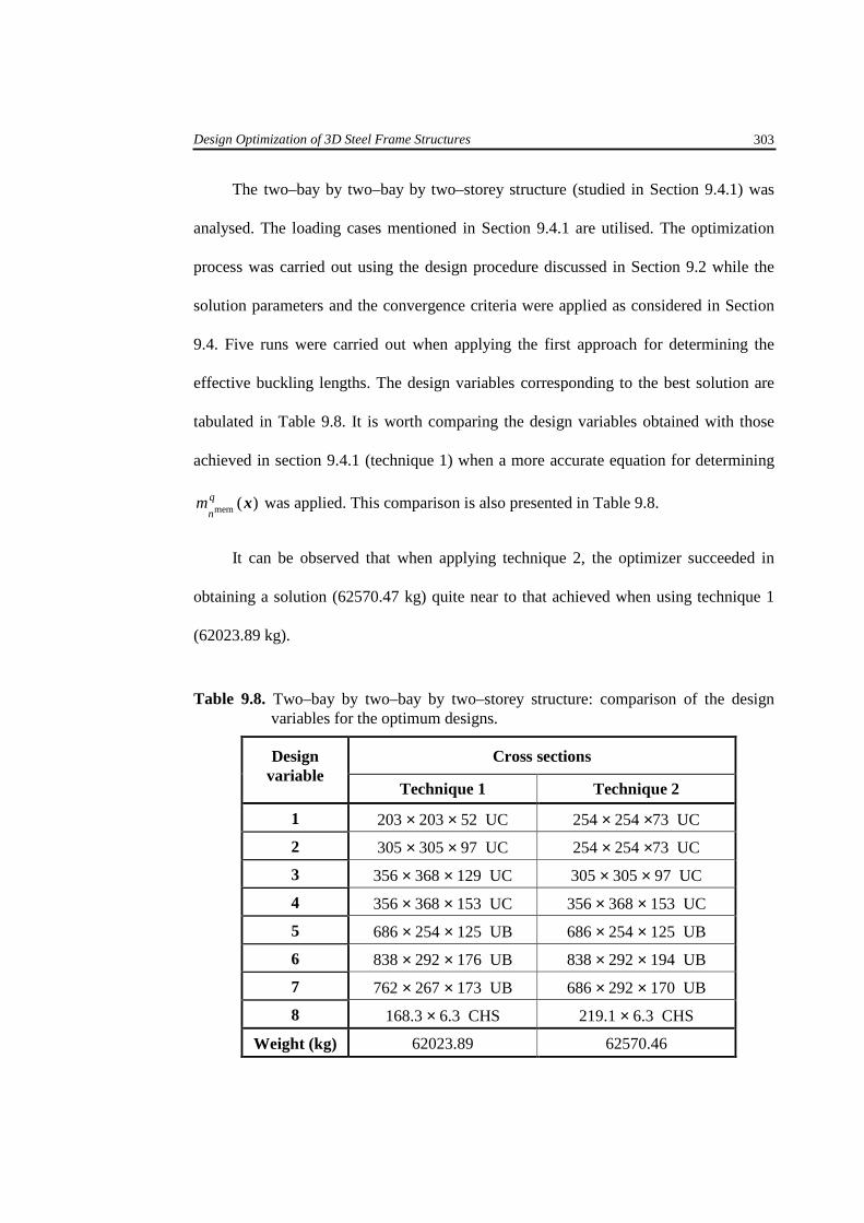
It can be observed that when applying technique 2, the optimizer succeeded in
obtaining a solution (62570.47 kg) quite near to that achieved when using technique 1
(62023.89 kg).
Table 9.8. Two–bay by two–bay by two–storey structure: comparison of the design variables for the optimum designs.
Cross sections Design var iable
Technique 1 Technique 2
1 203 × 203 × 52 UC 254 × 254 ×73 UC
2 305 × 305 × 97 UC 254 × 254 ×73 UC
3 356 × 368 × 129 UC 305 × 305 × 97 UC
4 356 × 368 × 153 UC 356 × 368 × 153 UC
5 686 × 254 × 125 UB 686 × 254 × 125 UB
6 838 × 292 × 176 UB 838 × 292 × 194 UB
7 762 × 267 × 173 UB 686 × 292 × 170 UB
8 168.3 × 6.3 CHS 219.1 × 6.3 CHS
Weight (kg) 62023.89 62570.46

Design Optimization of 3D Steel Frame Structures
304
The convergence characteristics were also examined. This was achieved by
plotting the changes of the best design with the number of generations performed for
each run as shown in Figure 9.11.
Figure 9.11. Two–bay by two–bay by two–storey structure: best design versus generation number
At this stage, the structural weight has been optimized and the section of each
member has been determined. The next step is to validate the code checks using CSC
software. This is achieved by using the following proceduce:
1) In S–FRAME, the structural geometry, member sections and loading cases are
defined. Then, the bending moments, shear forces, and nodal displacements are
calculated according to the analysis type presupposed (linear analysis).
2) Starting the S–STEEL program. The design checks are then carried out.
3) The design results are then displayed on a separate window as shown in Figure 9.12.
50000
70000
90000
110000
130000
150000
0 10 20 30 40 50 60 70 80 90
First runSecond runThird runFourth runFifth run
Generation number
Bes
t des
ign
(kg)
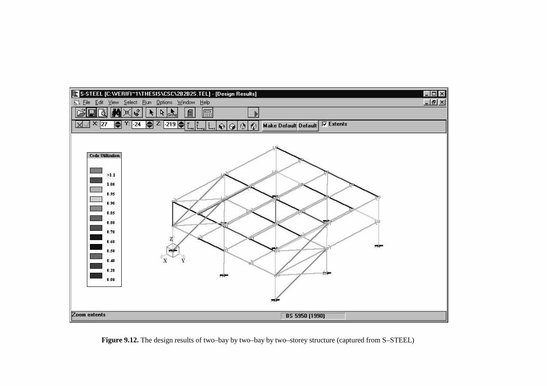
Figure 9.12. The design results of two–bay by two–bay by two–storey structure (captured from S–STEEL)
Design Optimization of 3D Steel Frame structures
306
In this figure, the design checks of each member are indicated in colour in which
the code utilisation menu gives the range for of each colour. It can be observed that most
of the members reach their maximum capacities. This indicates that the developed
algorithm is successfully incorporated in design optimization. It is worth noting that the
design results vary between 0.7 and 1.0.
9.6 Concluding remarks
Design optimization technique based on GA was presented for 3D steel frame structures
where the structures were subjected to multiple loading conditions. The design method
obtained a 3D steel frame structure with the least weight by selecting appropriate
sections for beams, columns and bracing members from the British standard for
universal beam sections, universal column sections and circular hollow sections. The
following concluding remarks can be made.
1) It has been proven that the developed GA approach can be successfully incorporated
in design optimization in which the structural members have to be selected from the
available standard sections while the design satisfies the design criteria. This
indicates that the developed approach can be utilised by a practising designers.
2) In the present chapter, the skills and experience of the designer have been reflected
in the optimization problem by imposing constraints on the second moment of area
of two adjacent columns in two adjacent storey levels. This can be implemented
using other constraints such as sectional dimensions, sectional area, etc. This
indicates that the optimizer is able to treat different practical constraints depending
on the nature of the problem.
3) It has been shown that the developed GA provides the designer with more than one
solution to choose from, and the difference between them was small. This could be
Design Optimization of 3D Steel Frame structures
307
an advantage when a designer needs to choose an appropriate solution depending on
the availability of the sections.
4) From Tables 9.4 and 9.7, it can be observed that the same sections have been
obtained for different members of a structure even though these members are linked
to different design variables. This indicates that it can be beneficial to include the
grouping of structural members as an additional criterion in the formulation of the
design optimization problem.
5) In the present study, computation of the effective buckling length has been
automated and included in the developed algorithm. This was achieved by
employing three different approaches.
Application of a modified GA to design optimization of structural steelwork allows
the best set from an appropriate catalogue of steel cross sections to be chosen. The
optimizer has been linked to a commercial finite element code and the British codes of
practice in order to obtain optimum designs accepted by practising structural engineers.