Embed Size (px)
Citation preview
Design of timber-concrete composite structures
Editors: Alfredo Dias, Jörg Schänzlin and Philipp Dietsch

Design of timber-concrete composite structures A state-of-the-art report by COST Action FP1402 / WG 4
With contributions by: Alfredo Dias, Massimo Fragiacomo, Kiril Gramatikov, Benjamin Kreis, Frank Kupferle, Sandra Monteiro, Jaroslav Sandanus, Jörg Schänzlin, Kay-Uwe Schober, Wendel Sebastian, Kristian Sogel
Editors: Alfredo Dias, Jörg Schänzlin, Philipp Dietsch

This publication is based upon work from COST Action FP1402, supported by COST (European Cooperation in Science and Technology).
COST (European Cooperation in Science and Technology) is a funding agency for research and innovation networks. Our Actions help connect research initiatives across Europe and enable scientists to grow their ideas by sharing them with their peers. This boosts their research, career and innovation. www.cost.eu
No permission to reproduce or utilise the contents of this book by any means is necessary, other than in the case of images, diagrams or other material from other copyright holders. In such cases, permission of the copyright holders is required. This book may be cited as: Dias, A., Schänzlin, J., Dietsch, P. (eds.), Design of timber-concrete composite structures: A state-of-the-art report by COST Action FP1402 / WG 4, Shaker Verlag Aachen, 2018.
Neither the COST Office nor any person acting on its behalf is responsible for the use which might be made of the information contained in this publication. The COST Office is not responsible for the external websites referred to in this publica-tion.
Copyright Shaker 2018 Printed in Germany ISBN 978-3-8440-6145-1 ISSN 0945-067X
Shaker Verlag GmbH · P.O. BOX 101818 · D-52018 Aachen
Phone: 0049/2407/9596-0 · Telefax: 0049/2407/9596-9
Internet: www.shaker.de · e-mail: [email protected]
Foreword
Timber-concrete composite structures are one alternative to common slab systems, since the advantages of pure timber slabs are combined with the advantages of pure concrete slabs. In order to benefit from these advantages, the systems have to be designed, considering the special properties and influences on the load carrying be-haviour and the deformation behaviour of this type of composite systems in the short term as well as in the long term. Despite these special requests for the design-er, timber-concrete composite structures are already used. Therefore a lot of re-search work and development have been done within whole Europe on this field.
The aim of this document is to report the state of the art in terms of research and practice of Timber-Concrete Composite (TCC) systems, in order to summarize the existing knowledge in the single countries and to develop a common understanding of the design of TCC.
This report was made within the framework of WG4-Hybrid Structures within COST Action FP1402. It intends to reflect the information and studies available around the world, but especially in Europe through the active contribution and par-ticipation of experts from various countries involved in this Action.
This state-of-the-art report reflects parts of the work and the discussions within in WG4 and will cover the relevant issues, such as
Input values Connection Evaluation of forces in the short and long term Design examples Methods for the evaluation of forces
However time is passing by, new developments will take place and new questions will be asked and solved, so this report can only present the current state of the art.
Alfredo Dias, Jörg Schänzlin, Chairs of Working Group 4, COST FP 1402
Philipp Dietsch, Chair, COST FP 1402

Table of contents 1. Introduction ........................................................................................................ 17
2. Input values ........................................................................................................ 21
2.1 General ......................................................................................................... 21
2.2 Dimensions ................................................................................................... 21
2.3 Material properties ....................................................................................... 21
2.4 Loads ............................................................................................................ 21
2.4.1 External loads ................................................................................. 21
2.4.2 Internal loads .................................................................................. 28
3. Connection .......................................................................................................... 33
3.1 Connection types .......................................................................................... 33
3.1.1 Introduction .................................................................................... 33
3.1.2 Dowel type fasteners ...................................................................... 34
3.1.3 Notches ........................................................................................... 35
3.1.4 Other connection types ................................................................... 36
3.1.4.1 General ............................................................................................. 36
3.1.4.2 Friction based connections ............................................................... 37
3.1.4.3 Adhesive-bonded timber-concrete composites ................................ 40
3.1.4.4 Concrete-type adhesives .................................................................. 41
3.1.4.5 Reversible system............................................................................. 43
3.2 Mechanical properties .................................................................................. 43
3.2.1 Introduction .................................................................................... 43
3.2.2 Stiffness .......................................................................................... 44
3.2.3 Strength ........................................................................................... 44
3.2.4 Ductility .......................................................................................... 44
3.3 Code Rules and Guidelines available ........................................................... 45
3.3.1 Introduction .................................................................................... 45
3.3.2 Eurocode 5 ...................................................................................... 45
3.3.3 Australia and New Zealand design Guidelines .............................. 47
3.3.4 USA – AASHO/AASTHO codes ................................................... 48
3.3.5 Canadian Highway Bridge Design Code........................................ 49
3.3.6 Brazil - Manual for the design of timber bridges ........................... 50
3.4 Assessment based on testing ........................................................................ 50
3.4.1 Test specimen configuration........................................................... 50
3.4.2 Load protocol and standards ........................................................... 52
3.4.3 Limitation of the experimental assessment tools ........................... 54
3.5 Determination based on calculation ............................................................. 54
3.5.1 General ............................................................................................ 54
3.5.2 Dowel-type fasteners ...................................................................... 55
3.5.2.1 Load Carrying Capacity ................................................................... 55
3.5.2.2 Stiffness ............................................................................................ 57
3.5.3 Inclined screws ............................................................................... 59
3.5.3.1 General ............................................................................................. 59
3.5.3.2 Load carrying capacity ..................................................................... 59
3.5.3.3 Stiffness ............................................................................................ 60
3.5.4 Notched Connections ...................................................................... 60
3.5.4.1 General ............................................................................................. 60
3.5.4.2 Load Carrying Capacity ................................................................... 62
3.5.4.3 Stiffness ............................................................................................ 62
3.5.5 Connections with Interlayer ........................................................... 62
3.5.6 Load-Slip models ............................................................................ 64
3.5.7 Finite Element Method models (FEM models) .............................. 65
3.6 Proprietary connection systems ................................................................... 66
3.6.1 General ............................................................................................ 66
3.6.2 SFS VB screws ............................................................................... 66
3.6.3 Tecnaria connectors ........................................................................ 67
3.6.4 ASSY plus VG screws .................................................................... 68
3.6.5 HBV Shear connector ..................................................................... 69
3.6.6 Parameters indicated in the Technical approvals ........................... 70
4. Evaluation of the forces ...................................................................................... 71
4.1 Preface .......................................................................................................... 71
4.2 Influences on the determination of the internal forces................................. 71
4.3 Determination of forces in the short term .................................................... 72
4.3.1 Consideration of the flexibility of the joint and the different cross section properties ............................................................................................... 72
4.3.2 Different inelastic strains ................................................................ 74
4.3.2.1 Influence on the internal forces ........................................................ 74
4.3.2.2 Influence of the yielding of the connectors ...................................... 77
4.3.3 Modelling the deformability of the joint ........................................ 78
4.3.3.1 General ............................................................................................. 78
4.3.3.2 Maximum spacing ............................................................................ 84
4.3.3.3 Extension of EN 1995 Annex B ....................................................... 87
4.3.4 Cracking of concrete and moment-rotation relation ...................... 94
4.3.4.1 Effect on the stiffness ....................................................................... 94
4.3.4.2 Is the normal design process of the concrete cross section applicable in timber-concrete-composite systems? ......................................................... 97
4.3.5 Stress-strain relation for the evaluation of internal forces ........... 101
4.3.6 Effective width ............................................................................. 102
4.3.7 Vibrations ..................................................................................... 105
4.4 Long term behaviour / consideration of creep and shrinkage .................... 106
4.4.1 Creep and shrinkage ..................................................................... 106
4.4.2 Development of the creep strain over time .................................. 107
4.4.3 Composite creep coefficients ....................................................... 112
4.4.4 Consideration of an effective shrinkage value ............................. 124
4.5 Design process ........................................................................................... 126
5. Design examples ............................................................................................... 129
5.1 General ....................................................................................................... 129
5.2 TCC beam verification according to the [EN 1995-1-1]/Annex B ............ 129
5.2.1 Basic information ......................................................................... 129
5.2.1.1 Cross section dimensions and material properties ......................... 129
5.2.1.1.1 Concrete slab – concrete grade C25/30 .................................... 129
5.2.1.1.2 Permanent formwork (interlayer) – OSB plates ....................... 129
5.2.1.1.3 Timber joist – KVH grade C24 ................................................. 130
5.2.1.2 Connection properties .................................................................... 130
5.2.2 Loads ............................................................................................ 131
5.2.3 Static scheme and internal forces analysis ................................... 131
5.2.4 Verification of the TCC beam at ultimate limit states (ULS) at the beginning of the lifetime ................................................................................. 131
5.2.4.1 Material properties ......................................................................... 131
5.2.4.1.1 Part 1 – concrete slab ................................................................ 131
5.2.4.1.2 Part 2 – timber joist ................................................................... 131
5.2.4.2 Slip modulus and γ-factor .............................................................. 132
5.2.4.3 Effective bending stiffness ............................................................. 132
5.2.4.4 Cross section analysis .................................................................... 132
5.2.4.4.1 Normal stresses in the concrete section .................................... 132
5.2.4.4.2 Normal stresses in the timber section ....................................... 133
5.2.4.4.3 Shear stresses in the timber section .......................................... 133
5.2.4.4.4 Verification of the fasteners ...................................................... 133
5.2.4.5 Cross section analysis considering only the effective compressed height of the concrete ................................................................................... 134
5.2.4.5.1 Effective bending stiffness ........................................................ 134
5.2.4.5.2 Stresses in the concrete section ................................................. 135
5.2.4.5.3 Stresses in the timber section .................................................... 135
5.2.4.5.4 Shear stresses in the timber section .......................................... 136
5.2.4.5.5 Verification of the fasteners ...................................................... 136
5.2.5 Verification of the TCC beam at ultimate limit states (ULS) at the end of the lifetime ............................................................................................ 136
5.2.5.1 Material properties ......................................................................... 136
5.2.5.1.1 Part 1 – concrete slab ................................................................ 136
5.2.5.1.2 Part 2 – timber joist ................................................................... 137
5.2.5.2 Slip modulus and γ-factor .............................................................. 137
5.2.5.3 Effective bending stiffness ............................................................. 137
5.2.5.4 Cross section analysis .................................................................... 138
5.2.5.4.1 Stresses in the concrete section ................................................. 138
5.2.5.4.2 Stresses in the timber section .................................................... 138
5.2.5.4.3 Shear stresses in the timber section .......................................... 139
5.2.5.4.4 Verification of the fasteners ...................................................... 139
5.2.6 Verification of the TCC beam at serviceability limit states (SLS) at the beginning of the lifetime ........................................................................... 139
5.2.6.1 Material properties ......................................................................... 139
5.2.6.1.1 Part 1 – concrete slab ................................................................ 139
5.2.6.1.2 Part 2 – timber joist ................................................................... 140
5.2.6.2 Slip modulus and γ-factor .............................................................. 140
5.2.6.3 Effective bending stiffness ............................................................. 140
5.2.6.4 Deflection at the beginning of the lifetime .................................... 140
5.2.7 Verification of the TCC beam at serviceability limit states (SLS) at the end of the lifetime ...................................................................................... 140
5.2.7.1 Material properties ......................................................................... 140
5.2.7.1.1 Part 1 – concrete slab ................................................................ 140
5.2.7.1.2 Part 2 – timber joist ................................................................... 141
5.2.7.2 Slip modulus and γ-factor .............................................................. 141
5.2.7.3 Effective bending stiffness ............................................................. 141
5.2.7.4 Deflection at the end of the lifetime .............................................. 141
5.3 Design example according to the provisions proposed in this report ........ 142
5.3.1 Input values ................................................................................... 142
5.3.1.1 System ............................................................................................ 142
5.3.1.2 Concrete ......................................................................................... 143
5.3.1.2.1 Geometrical input values .......................................................... 143
5.3.1.2.2 Cross section parameters........................................................... 143
5.3.1.2.3 Material properties .................................................................... 143
5.3.1.3 Non-load-bearing interlayer ........................................................... 144
5.3.1.4 Timber ............................................................................................ 144
5.3.1.4.1 Geometrical input values .......................................................... 144
5.3.1.4.2 Cross section parameters........................................................... 144
5.3.1.4.3 Material properties .................................................................... 144
5.3.1.5 Connection properties .................................................................... 145
5.3.2 Loads ............................................................................................ 145
5.3.2.1 Design values of the loads ............................................................. 146
5.3.3 ULS-design at t = 0 years ............................................................. 147
5.3.3.1 Bending stiffness ............................................................................ 147
5.3.3.2 Consideration of inelastic strains ................................................... 148
5.3.3.3 Forces ............................................................................................. 148
5.3.3.3.1 External forces .......................................................................... 148
5.3.3.3.2 Internal forces of the single components .................................. 149
5.3.3.4 Stresses in the concrete section and verification ........................... 150
5.3.3.4.1 Stresses ...................................................................................... 150
5.3.3.4.2 Verification of the stresses in the concrete ............................... 151
5.3.3.5 Stresses in the timber cross section and verification ..................... 151
5.3.3.5.1 Normal stresses ......................................................................... 151
5.3.3.5.1.1 Stresses in the timber cross section and verification .......... 152
5.3.3.5.1.2 Verification of the normal stresses ..................................... 152
5.3.3.5.1.3 Check, whether time period of 3-7 years has to be checked (see Sec. 4.4.2) ........................................................................................ 152
5.3.3.5.2 Shear stresses ............................................................................ 152
5.3.3.5.2.1 Determination of the shear stresses .................................... 152
5.3.3.5.2.2 Verification of the shear ..................................................... 153
5.3.3.6 Connection ..................................................................................... 153
5.3.3.6.1 Forces in the connection ........................................................... 153
5.3.3.6.2 Verification of the connection .................................................. 154
5.3.4 SLS-design at t = 0 years .............................................................. 154
5.3.4.1 Loads .............................................................................................. 154
5.3.4.2 Effective bending stiffness ............................................................. 155
5.3.4.3 Effective bending stiffness with respect to the inelastic strains .... 155
5.3.4.4 Deformation ................................................................................... 156
5.3.5 ULS-design at t = 50 years ........................................................... 156
5.3.5.1 Bending stiffness ............................................................................ 156
5.3.5.2 Consideration of inelastic strains ................................................... 158
5.3.5.3 Forces ............................................................................................. 159
5.3.5.3.1 External forces .......................................................................... 159
5.3.5.3.2 Internal forces of the single components .................................. 159
5.3.5.4 Stresses in the concrete section and verification ........................... 160
5.3.5.4.1 Stresses ...................................................................................... 160
5.3.5.4.2 Verification of the stresses in the concrete ............................... 160
5.3.5.5 Stresses in the timber cross section and verification ..................... 161
5.3.5.5.1 Normal stresses ......................................................................... 161
5.3.5.5.1.1 Stresses in the timber cross section and verification .......... 161
5.3.5.5.1.2 Verification of the normal stresses ..................................... 161
5.3.5.5.1.3 Check, whether time period of 3-7 years has to be checked (see Sec. 4.4.2) ........................................................................................ 161
5.3.5.5.2 Shear stresses ............................................................................ 162
5.3.5.5.2.1 Determination of the shear stresses .................................... 162
5.3.5.5.2.2 Verification of the shear ..................................................... 162
5.3.5.6 Connection ..................................................................................... 163
5.3.5.6.1 Forces in the connection ........................................................... 163
5.3.5.6.2 Verification of the connection .................................................. 163
5.3.6 SLS-design at t = 50 years ............................................................ 164
5.3.6.1 Loads .............................................................................................. 164
5.3.6.2 effective bending stiffness ............................................................. 164
5.3.6.3 Effective bending stiffness with respect to the inelastic strains .... 164
5.3.6.4 Deformation ................................................................................... 165
5.3.7 ULS-design at t = 3-7 years .......................................................... 166
5.3.7.1 Bending stiffness ............................................................................ 166
5.3.7.2 Consideration of inelastic strains ................................................... 167
5.3.7.3 Forces ............................................................................................. 168
5.3.7.3.1 External forces .......................................................................... 168
5.3.7.3.2 Internal forces of the single components .................................. 169
5.3.7.4 Stresses in the concrete section and verification ........................... 169
5.3.7.4.1 Stresses ...................................................................................... 169
5.3.7.4.2 Verification of the stresses in the concrete ............................... 170
5.3.7.5 Stresses in the timber cross section and verification ..................... 170
5.3.7.5.1 Normal stresses ......................................................................... 170
5.3.7.5.1.1 Stresses in the timber cross section and verification .......... 170
5.3.7.5.1.2 Verification of the normal stresses ..................................... 171
5.3.7.5.2 Shear stresses ............................................................................ 171
5.3.7.5.2.1 Determination of the shear stresses .................................... 171
5.3.7.5.2.2 Verification of the shear ..................................................... 171
5.3.7.6 Connection ..................................................................................... 172
5.3.7.6.1 Forces in the connection ........................................................... 172
5.3.7.6.2 Verification of the connection .................................................. 172
5.3.8 SLS-design at t = 3-7 years .......................................................... 173
6. Summary, conclusions and outlook ................................................................. 175
6.1 Summary and conclusion ........................................................................... 175
6.2 Outlook ....................................................................................................... 176
7. References ........................................................................................................ 177
7.1 References .................................................................................................. 177
7.2 Additional references ................................................................................. 191
A Technical approvals .......................................................................................... 199
B Evaluation of the internal forces ...................................................................... 205
B.1 General ....................................................................................................... 205
B.2 Methods for the determination of the internal forces considering the deformability of the connectors ........................................................................... 207
B.2.1 General .................................................................................................. 207
B.2.2 Differential equation ............................................................................. 207
B.2.3 -method of EC 5 Annex B .................................................................. 216
B.2.4 Strut & Tie model ................................................................................. 220
B.2.5 Shear analogy method .......................................................................... 221
B.2.6 FE-modelling ........................................................................................ 227
B.2.7 Summary ............................................................................................... 228

16
17
1. Introduction
In timber-concrete-composite structures, a timber element is connected to the con-crete cross section by means of special connecting elements. In most cases the con-crete cross section is installed in the compression zone, whereas the timber is in-stalled in the tension zone.
Connecting timber with concrete provides the advantages of pure timber and pure concrete slabs. These advantages compared to a pure timber slab are:
Increased stiffness Increased load carrying capacity Improved sound insulation Reduced sensitivity concerning vibrations Simplified possibility to realize the horizontal bracing of the structure
Compared to a pure concrete slab the advantages are the following:
Reduced dead load Increase of re-growing materials and therefore less CO2 emissions Increase of prefabricated elements leading to a faster erection of the structure
and therefore to a lower influence of the surrounding conditions during the erection phase
Reduced volume of concrete, which leads to a faster building process and less volume to be transported on site
Reduced effort for the props/formwork since the load carrying capacity and the stiffness of the timber cross section is higher than the related properties of the prefabricated concrete elements
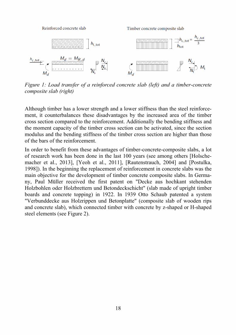
These advantages can only be used if the slab has a sufficient load carrying capaci-ty and a sufficient stiffness in order to fulfil the requirements. In concrete design, the tensile strength of concrete is often neglected and the reinforcement is installed to transfer the tensile stresses caused by bending. In the ultimate limit state the con-crete is cracked to about 2/3 of its height under bending. In timber-concrete compo-site structures, this cracked area is replaced by the timber cross section (see Figure 1).
18
Figure 1: Load transfer of a reinforced concrete slab (left) and a timber-concrete composite slab (right)
Although timber has a lower strength and a lower stiffness than the steel reinforce-ment, it counterbalances these disadvantages by the increased area of the timber cross section compared to the reinforcement. Additionally the bending stiffness and the moment capacity of the timber cross section can be activated, since the section modulus and the bending stiffness of the timber cross section are higher than those of the bars of the reinforcement.
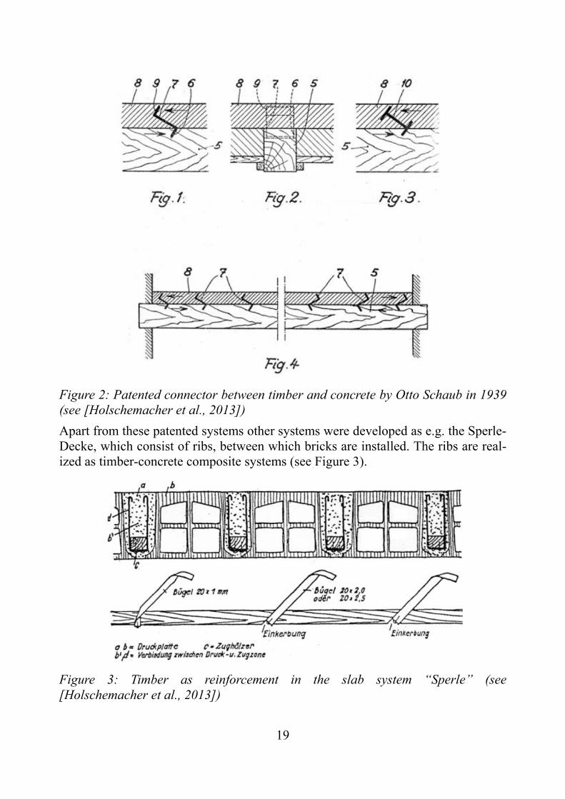
In order to benefit from these advantages of timber-concrete-composite slabs, a lot of research work has been done in the last 100 years (see among others [Holsche-macher et al., 2013], [Yeoh et al., 2011], [Rautenstrauch, 2004] and [Postulka, 1998]). In the beginning the replacement of reinforcement in concrete slabs was the main objective for the development of timber concrete composite slabs. In Germa-ny, Paul Müller received the first patent on "Decke aus hochkant stehenden Holzbohlen oder Holzbrettern und Betondeckschicht" (slab made of upright timber boards and concrete topping) in 1922. In 1939 Otto Schaub patented a system "Verbunddecke aus Holzrippen und Betonplatte" (composite slab of wooden rips and concrete slab), which connected timber with concrete by z-shaped or H-shaped steel elements (see Figure 2).
19
Figure 2: Patented connector between timber and concrete by Otto Schaub in 1939 (see [Holschemacher et al., 2013])
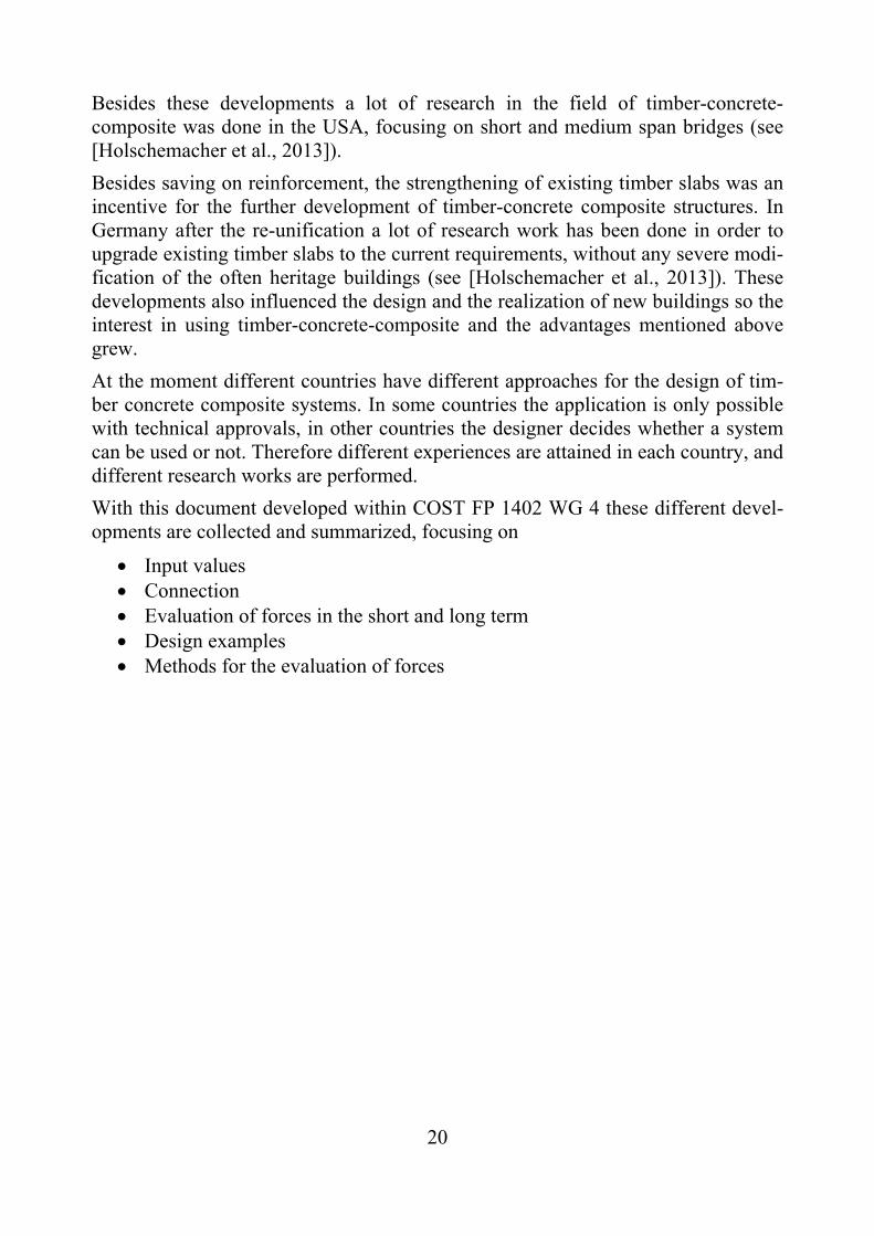
Apart from these patented systems other systems were developed as e.g. the Sperle-Decke, which consist of ribs, between which bricks are installed. The ribs are real-ized as timber-concrete composite systems (see Figure 3).
Figure 3: Timber as reinforcement in the slab system “Sperle” (see [Holschemacher et al., 2013])
20
Besides these developments a lot of research in the field of timber-concrete-composite was done in the USA, focusing on short and medium span bridges (see [Holschemacher et al., 2013]).
Besides saving on reinforcement, the strengthening of existing timber slabs was an incentive for the further development of timber-concrete composite structures. In Germany after the re-unification a lot of research work has been done in order to upgrade existing timber slabs to the current requirements, without any severe modi-fication of the often heritage buildings (see [Holschemacher et al., 2013]). These developments also influenced the design and the realization of new buildings so the interest in using timber-concrete-composite and the advantages mentioned above grew.
At the moment different countries have different approaches for the design of tim-ber concrete composite systems. In some countries the application is only possible with technical approvals, in other countries the designer decides whether a system can be used or not. Therefore different experiences are attained in each country, and different research works are performed.
With this document developed within COST FP 1402 WG 4 these different devel-opments are collected and summarized, focusing on
Input values Connection Evaluation of forces in the short and long term Design examples Methods for the evaluation of forces
21
2. Input values
2.1 General
In order to design timber-concrete-composite systems the appropriate input values have to been chosen. The input values can be divided into following groups
Dimensions Material properties Loads
2.2 Dimensions
In the evaluation of forces, the cross sectional dimensions and bending stiffness influence the internal forces. However no significant differences between the “nor-mal” design of pure timber or pure concrete structures compared to timber-concrete-composite systems exist. Therefore the common practice using the nomi-nal cross section dimensions are used for the design.
2.3 Material properties
In order to evaluate the internal forces, the material properties namely modulus of elasticity, (in some methods) the shear modulus and the stiffness of the connection influence the stress distribution. Since the “real” stresses and the “real” deformation should be evaluated, it is recommended to use the mean values of the material properties and not the modified modulus of elasticity e.g. by the partial material safety factor as it can be deducted from [EN 1995-1-1] Cl. 2.2.2, since the internal forces in the timber-concrete-composite cross section depend on the stiffness of the components. It has to be mentioned, that there are no studies available, discussing the influence of the variability of the Modulus of Elasticity on the internal forces, since e.g. overestimating the MoE of concrete leads to an underestimation of the internal forces in the timber cross section.
2.4 Loads
2.4.1 External loads
The loads due to dead loads and due to live loads have to be considered in the de-sign. The values are given in [EN 1991-1-1] and can be applied for the design of the structure. It is recommended to split between the (quasi) permanent and the short term loads in order to apply these loads in the short term as well as in the long term analysis, if the duration of the load is long enough to lead to creep defor-mations.
Although the external loads such as dead loads and / or live loads are the same as in pure timber or pure concrete structures, the process of erection may influence the loads as well as the load distribution.
Load distribution in the cross section: The loads are applied according to the erection process. Following situations have to be studied within the model-
22
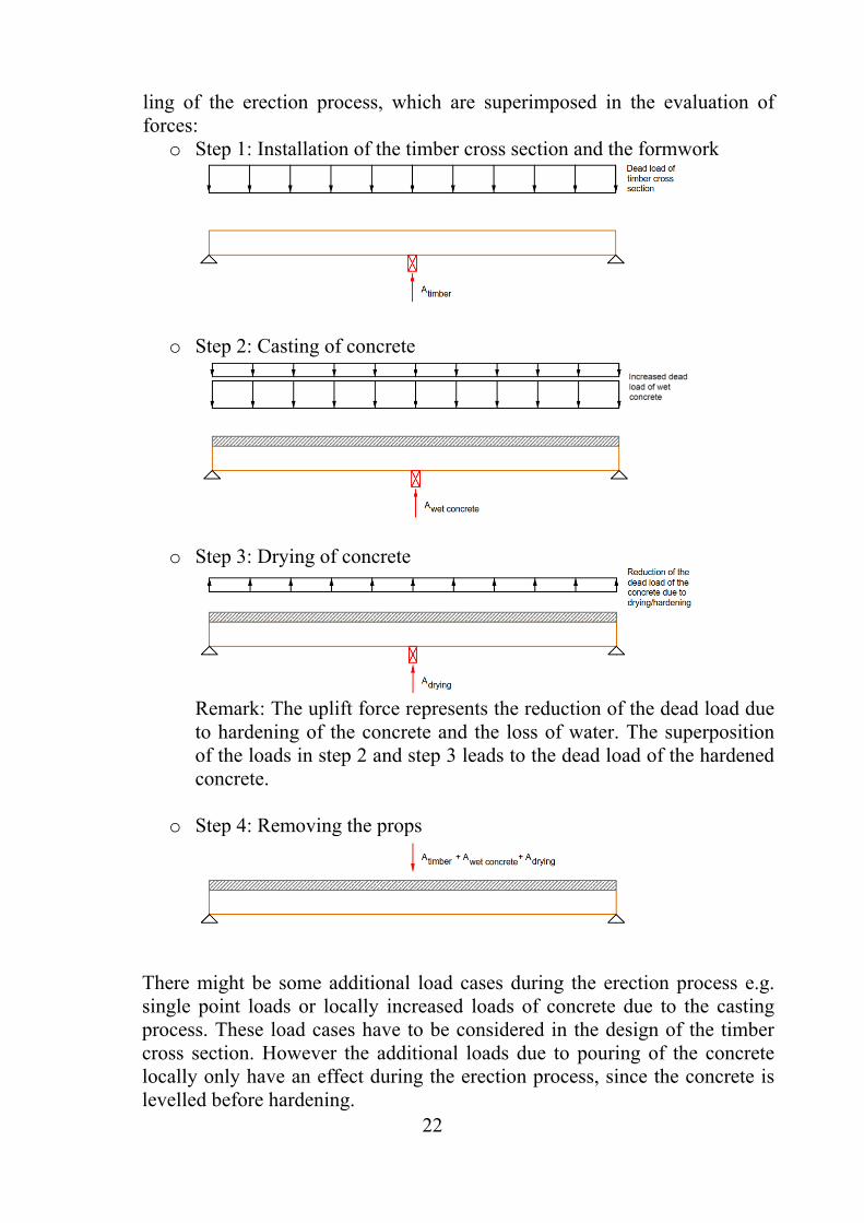
ling of the erection process, which are superimposed in the evaluation of forces:
o Step 1: Installation of the timber cross section and the formwork
o Step 2: Casting of concrete
o Step 3: Drying of concrete
Remark: The uplift force represents the reduction of the dead load due to hardening of the concrete and the loss of water. The superposition of the loads in step 2 and step 3 leads to the dead load of the hardened concrete.
o Step 4: Removing the props
There might be some additional load cases during the erection process e.g. single point loads or locally increased loads of concrete due to the casting process. These load cases have to be considered in the design of the timber cross section. However the additional loads due to pouring of the concrete locally only have an effect during the erection process, since the concrete is levelled before hardening.

23
In order to model the erection process at least four situations have to be su-perimposed considering the stiffness of the concrete in every situation (see Table 1).
Table 1: Load bearing cross section in every design situation
Situation Load bearing cross section
Step 1: Installation Only timber cross section
Step 2: Casting Only timber cross section
Step 3: Drying of concrete Composite cross section
Step 4: Removing of the props Composite cross section
As a result the internal forces have to be determined with respect to the erection process. This can be done by applying the changes of the loads from step to step and by superimposing the single states.
For the example shown in the steps 1 to 4 the internal forces develop in principle according to the following steps:
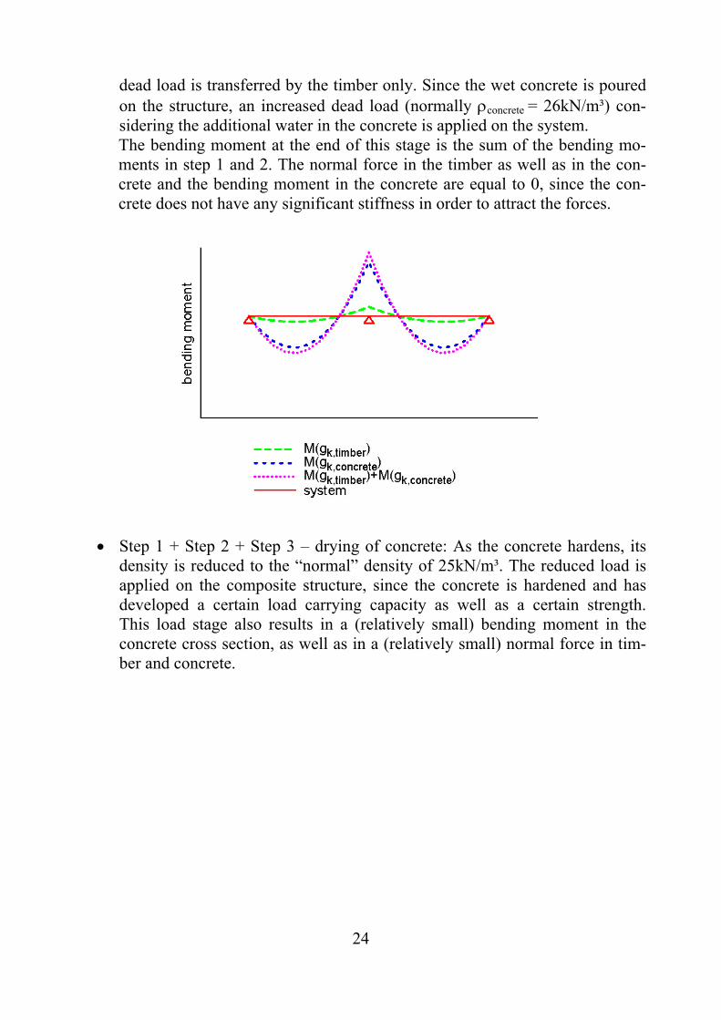
Step 1 – installation: The bending moment in the timber cross section is caused by the dead load of the timber element. The props act as support of the beam. The normal force is equal to 0, since in this example no external normal force exists.
Step 1 + Step 2 – casting of concrete: The concrete is poured on the timber elements. Since the concrete does not have any stiffness at this stage, the
24
dead load is transferred by the timber only. Since the wet concrete is poured on the structure, an increased dead load (normally concrete = 26kN/m³) con-sidering the additional water in the concrete is applied on the system. The bending moment at the end of this stage is the sum of the bending mo-ments in step 1 and 2. The normal force in the timber as well as in the con-crete and the bending moment in the concrete are equal to 0, since the con-crete does not have any significant stiffness in order to attract the forces.
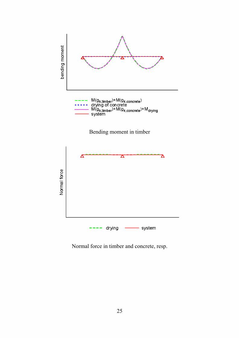
Step 1 + Step 2 + Step 3 – drying of concrete: As the concrete hardens, its density is reduced to the “normal” density of 25kN/m³. The reduced load is applied on the composite structure, since the concrete is hardened and has developed a certain load carrying capacity as well as a certain strength. This load stage also results in a (relatively small) bending moment in the concrete cross section, as well as in a (relatively small) normal force in tim-ber and concrete.
25
Bending moment in timber
Normal force in timber and concrete, resp.
26
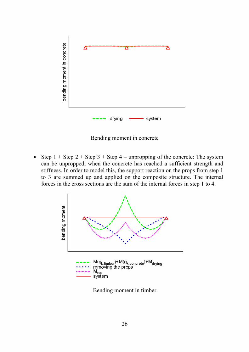
Bending moment in concrete
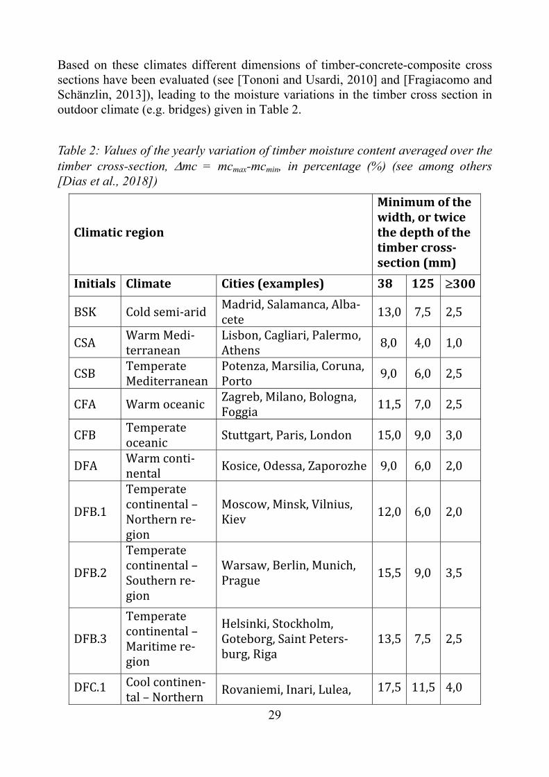
Step 1 + Step 2 + Step 3 + Step 4 – unpropping of the concrete: The system can be unpropped, when the concrete has reached a sufficient strength and stiffness. In order to model this, the support reaction on the props from step 1 to 3 are summed up and applied on the composite structure. The internal forces in the cross sections are the sum of the internal forces in step 1 to 4.
Bending moment in timber
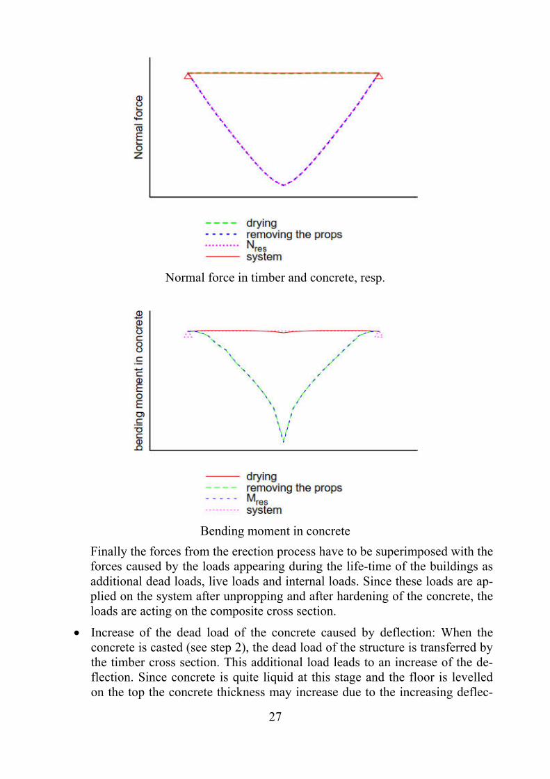
27
Normal force in timber and concrete, resp.
Bending moment in concrete
Finally the forces from the erection process have to be superimposed with the forces caused by the loads appearing during the life-time of the buildings as additional dead loads, live loads and internal loads. Since these loads are ap-plied on the system after unpropping and after hardening of the concrete, the loads are acting on the composite cross section.
Increase of the dead load of the concrete caused by deflection: When the concrete is casted (see step 2), the dead load of the structure is transferred by the timber cross section. This additional load leads to an increase of the de-flection. Since concrete is quite liquid at this stage and the floor is levelled on the top the concrete thickness may increase due to the increasing deflec-

28
tion. This increasing thickness leads to a higher dead load of the concrete slab, which should be considered in the design.
2.4.2 Internal loads
Since the concrete cross section is connected to the timber cross section, every rela-tive change in the cross sectional dimensions especially in span direction leads to eigenstresses. Since timber is more or less brittle in tension, these eigenstresses can influence the load carrying capacity of the whole structure. These eigenstresses are caused by
Temperature variation Moisture variation of the timber cross section Shrinkage of concrete
For the design the temperature variation is given in [EN 1991-1-5] whereas the moisture variation is defined in the Service classes according to [EN 1995-1-1]. However the Service classes only represent the range of equilibrium moisture con-tents, so the moisture variation e.g. within one year cannot be derived from these values. In [Tononi and Usardi, 2010] (see [Fragiacomo and Schänzlin, 2013]) the moisture content is evaluated for different climates. These climates are defined in the Köppen-Geiger-climatic map in Europe (see Figure 4).
Figure 4: Köppen-Geiger climatic map of Europe
29
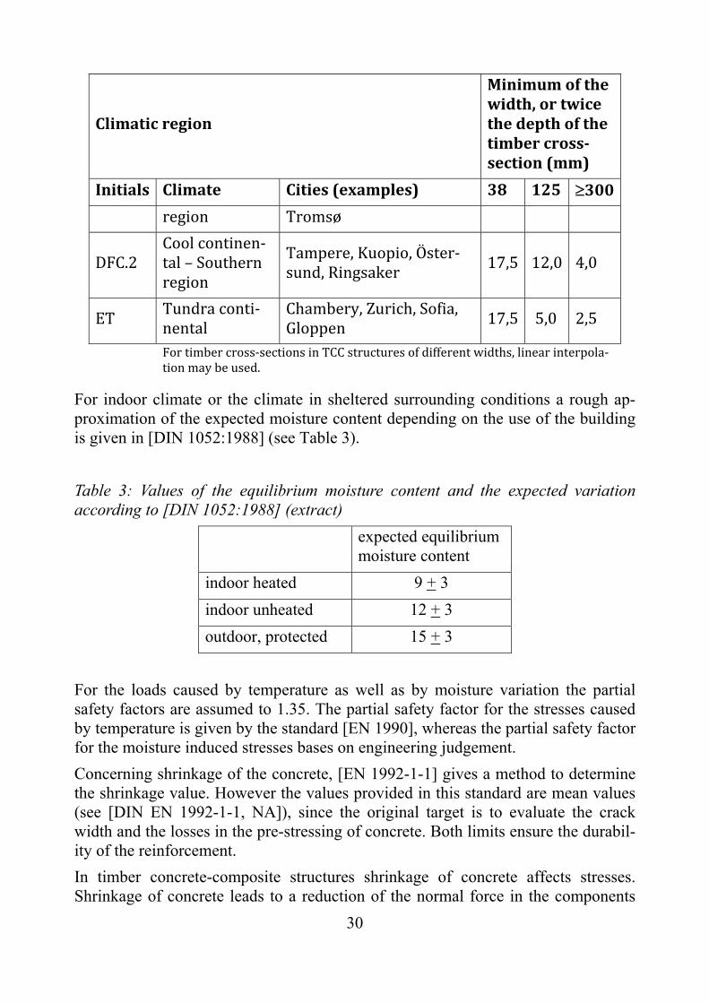
Based on these climates different dimensions of timber-concrete-composite cross sections have been evaluated (see [Tononi and Usardi, 2010] and [Fragiacomo and Schänzlin, 2013]), leading to the moisture variations in the timber cross section in outdoor climate (e.g. bridges) given in Table 2.
Table 2: Values of the yearly variation of timber moisture content averaged over the timber cross-section, mc = mcmax-mcmin, in percentage (%) (see among others [Dias et al., 2018])
Climaticregion
Minimumofthewidth,ortwicethedepthofthetimbercross‐section(mm)
Initials Climate Cities(examples) 38 125 300
BSK Coldsemi‐aridMadrid,Salamanca,Alba‐cete
13,0 7,5 2,5
CSAWarmMedi‐terranean
Lisbon,Cagliari,Palermo,Athens 8,0 4,0 1,0
CSBTemperateMediterranean
Potenza,Marsilia,Coruna,Porto
9,0 6,0 2,5
CFA Warmoceanic Zagreb,Milano,Bologna,Foggia
11,5 7,0 2,5
CFBTemperateoceanic
Stuttgart,Paris,London 15,0 9,0 3,0
DFA Warmconti‐nental
Kosice,Odessa,Zaporozhe 9,0 6,0 2,0
DFB.1
Temperatecontinental–Northernre‐gion
Moscow,Minsk,Vilnius,Kiev
12,0 6,0 2,0
DFB.2
Temperatecontinental–Southernre‐gion
Warsaw,Berlin,Munich,Prague
15,5 9,0 3,5
DFB.3
Temperatecontinental–Maritimere‐gion
Helsinki,Stockholm,Goteborg,SaintPeters‐burg,Riga
13,5 7,5 2,5
DFC.1 Coolcontinen‐tal–Northern
Rovaniemi,Inari,Lulea, 17,5 11,5 4,0
30
Climaticregion
Minimumofthewidth,ortwicethedepthofthetimbercross‐section(mm)
Initials Climate Cities(examples) 38 125 300
region Tromsø
DFC.2Coolcontinen‐tal–Southernregion
Tampere,Kuopio,Öster‐sund,Ringsaker
17,5 12,0 4,0
ETTundraconti‐nental
Chambery,Zurich,Sofia,Gloppen
17,5 5,0 2,5
Fortimbercross‐sectionsinTCCstructuresofdifferentwidths,linearinterpola‐tionmaybeused.
For indoor climate or the climate in sheltered surrounding conditions a rough ap-proximation of the expected moisture content depending on the use of the building is given in [DIN 1052:1988] (see Table 3).
Table 3: Values of the equilibrium moisture content and the expected variation according to [DIN 1052:1988] (extract)
expected equilibrium moisture content
indoor heated 9 + 3
indoor unheated 12 + 3
outdoor, protected 15 + 3
For the loads caused by temperature as well as by moisture variation the partial safety factors are assumed to 1.35. The partial safety factor for the stresses caused by temperature is given by the standard [EN 1990], whereas the partial safety factor for the moisture induced stresses bases on engineering judgement.
Concerning shrinkage of the concrete, [EN 1992-1-1] gives a method to determine the shrinkage value. However the values provided in this standard are mean values (see [DIN EN 1992-1-1, NA]), since the original target is to evaluate the crack width and the losses in the pre-stressing of concrete. Both limits ensure the durabil-ity of the reinforcement.
In timber concrete-composite structures shrinkage of concrete affects stresses. Shrinkage of concrete leads to a reduction of the normal force in the components
31
and an increase of the bending moment in the timber as well as in the concrete cross section. Since the utilization of the cross section is determined by the sum of the utilization of the single parts
, ,
, ,
,
,1.0 (1)
and the strength in bending , is higher than the tensile strength , , , the final utilization of the cross section does not necessarily increase if the bending mo-ment increases due to shrinkage of concrete. In this case, the normal force in the timber cross section decreases, when the bending moment increases, since the ex-ternal bending moment is constant over time
⋅8
⋅ (2)
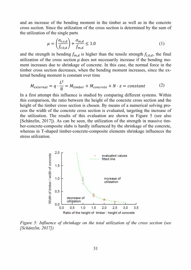
In a first attempt this influence is studied by comparing different systems. Within this comparison, the ratio between the height of the concrete cross section and the height of the timber cross section is chosen. By means of a numerical solving pro-cess the width of the concrete cross section is evaluated, targeting the increase of the utilization. The results of this evaluation are shown in Figure 5 (see also [Schänzlin, 2017]). As can be seen, the utilization of the strength in massive tim-ber-concrete-composite slabs is hardly influenced by the shrinkage of the concrete, whereas in T-shaped timber-concrete-composite elements shrinkage influences the stress utilization.
Figure 5: Influence of shrinkage on the total utilization of the cross section (see [Schänzlin, 2017])
32
In [EN 1992-1-1] shrinkage values are given; however the values provided are the mean values. [DIN EN 1992-1-1, NA] states that the shrinkage values given in [EN 1992-1-1] are the mean value and the coefficient of variation of about 30% has to be considered in the evaluation. [JCSS, 2001] states that shrinkage of concrete can be modelled by means of the log-normal-distribution.
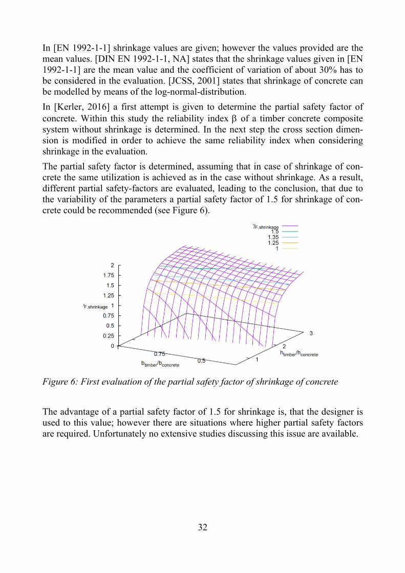
In [Kerler, 2016] a first attempt is given to determine the partial safety factor of concrete. Within this study the reliability index of a timber concrete composite system without shrinkage is determined. In the next step the cross section dimen-sion is modified in order to achieve the same reliability index when considering shrinkage in the evaluation.
The partial safety factor is determined, assuming that in case of shrinkage of con-crete the same utilization is achieved as in the case without shrinkage. As a result, different partial safety-factors are evaluated, leading to the conclusion, that due to the variability of the parameters a partial safety factor of 1.5 for shrinkage of con-crete could be recommended (see Figure 6).
Figure 6: First evaluation of the partial safety factor of shrinkage of concrete
The advantage of a partial safety factor of 1.5 for shrinkage is, that the designer is used to this value; however there are situations where higher partial safety factors are required. Unfortunately no extensive studies discussing this issue are available.
33
3. Connection
3.1 Connection types
3.1.1 Introduction
The connection system is a critical component in the conception, design and per-formance of TCC systems. Due to the indeterminate nature of these systems it affects the stress distribution and the deformations, consequently the whole de-sign. In principle, from the mechanical performance point of view, the ideal connection should be: i) strong enough to transmit the shear forces developed at the interface, ii) stiff enough to transmit the load with a limited slip at the inter-face, iii) ductile enough to allow full load distribution and avoid failure on the fasteners. Additionally, other variables need to be taken into account such as the connection cost, feasibility in practice or complexity.
The connection systems available only fulfil part of the mechanical performance parameters listed for an ideal connection. This is particularly the case regarding the stiffness, since the connection slip will not be negligible for most of the TCC systems. This flexibility affects not only the connection design but also the whole system analysis once the interface slip needs to be taken into account and simple models such as the transformed section method are not valid. Conse-quently, the choice of a particular type of connection will significantly influence the overall behaviour of the composite system, being a critical component that must be carefully conceived and designed.
Due to this aspect, many research works have been performed from the early ages of use of the TCC systems, addressing many aspects related to connections (see [Richart and Williams, 1943] and [Baldock and McCullough, 1941]).
The TCC systems can be seen as a natural development of the timber systems. It was originally focused on high load bearing structures and motivated by the lower cost, higher short and long term performance and scarcity of steel during the two world wars (see [McCullough, 1934]). Consequently many connection systems are based on timber-timber connections (see [Richart and Williams, 1943]). Most of these connection systems use steel fasteners such as screws, nails or dowels, (see [McCullough, 1943], [RILEM-CT-111-CST, 1992] and [Richart and Williams, 1943]).
From the early times up to now many of the studies focused on development and characterization of specific connection systems. By use of those studies, a data-base was created. This work was done at the Civil Engineering Department of the University of Coimbra and served primarily as the base of a statistic study carried out by [Monteiro et al., 2010], being now updated in order to include al-so recent studies. In total it includes around 60 references. The complete refer-ence list is given in the Annex.
34
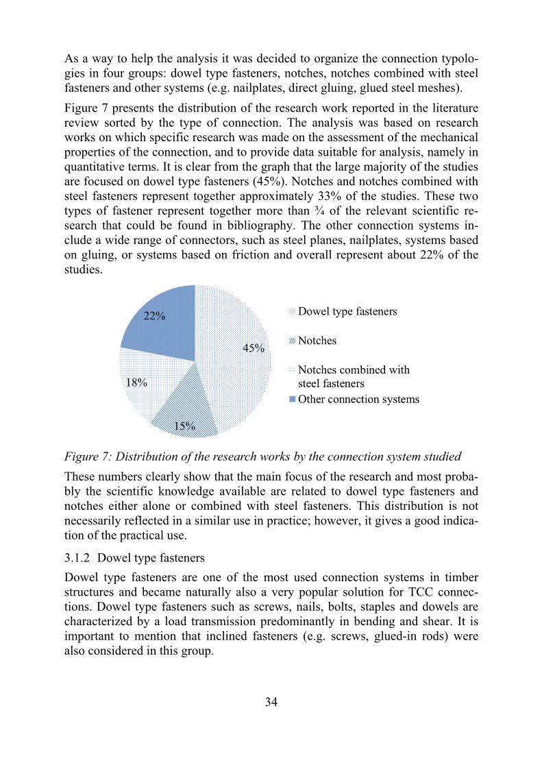
As a way to help the analysis it was decided to organize the connection typolo-gies in four groups: dowel type fasteners, notches, notches combined with steel fasteners and other systems (e.g. nailplates, direct gluing, glued steel meshes).
Figure 7 presents the distribution of the research work reported in the literature review sorted by the type of connection. The analysis was based on research works on which specific research was made on the assessment of the mechanical properties of the connection, and to provide data suitable for analysis, namely in quantitative terms. It is clear from the graph that the large majority of the studies are focused on dowel type fasteners (45%). Notches and notches combined with steel fasteners represent together approximately 33% of the studies. These two types of fastener represent together more than ¾ of the relevant scientific re-search that could be found in bibliography. The other connection systems in-clude a wide range of connectors, such as steel planes, nailplates, systems based on gluing, or systems based on friction and overall represent about 22% of the studies.
Figure 7: Distribution of the research works by the connection system studied
These numbers clearly show that the main focus of the research and most proba-bly the scientific knowledge available are related to dowel type fasteners and notches either alone or combined with steel fasteners. This distribution is not necessarily reflected in a similar use in practice; however, it gives a good indica-tion of the practical use.
3.1.2 Dowel type fasteners
Dowel type fasteners are one of the most used connection systems in timber structures and became naturally also a very popular solution for TCC connec-tions. Dowel type fasteners such as screws, nails, bolts, staples and dowels are characterized by a load transmission predominantly in bending and shear. It is important to mention that inclined fasteners (e.g. screws, glued-in rods) were also considered in this group.
35
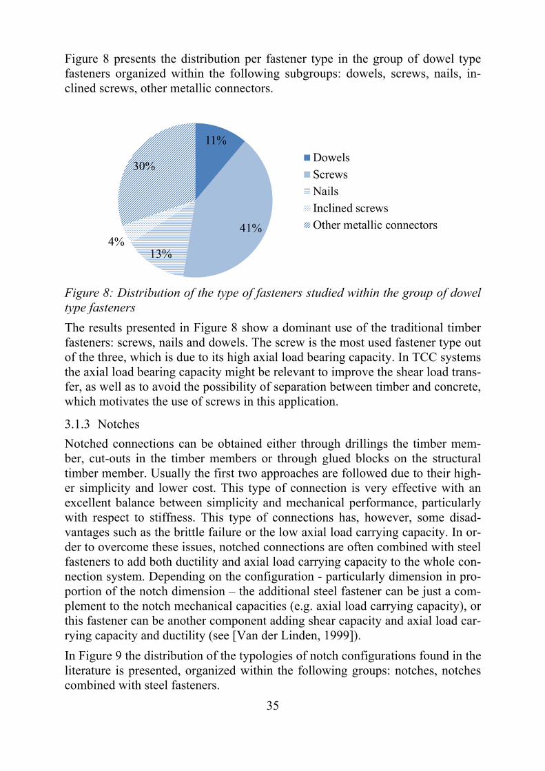
Figure 8 presents the distribution per fastener type in the group of dowel type fasteners organized within the following subgroups: dowels, screws, nails, in-clined screws, other metallic connectors.
Figure 8: Distribution of the type of fasteners studied within the group of dowel type fasteners
The results presented in Figure 8 show a dominant use of the traditional timber fasteners: screws, nails and dowels. The screw is the most used fastener type out of the three, which is due to its high axial load bearing capacity. In TCC systems the axial load bearing capacity might be relevant to improve the shear load trans-fer, as well as to avoid the possibility of separation between timber and concrete, which motivates the use of screws in this application.
3.1.3 Notches
Notched connections can be obtained either through drillings the timber mem-ber, cut-outs in the timber members or through glued blocks on the structural timber member. Usually the first two approaches are followed due to their high-er simplicity and lower cost. This type of connection is very effective with an excellent balance between simplicity and mechanical performance, particularly with respect to stiffness. This type of connections has, however, some disad-vantages such as the brittle failure or the low axial load carrying capacity. In or-der to overcome these issues, notched connections are often combined with steel fasteners to add both ductility and axial load carrying capacity to the whole con-nection system. Depending on the configuration - particularly dimension in pro-portion of the notch dimension – the additional steel fastener can be just a com-plement to the notch mechanical capacities (e.g. axial load carrying capacity), or this fastener can be another component adding shear capacity and axial load car-rying capacity and ductility (see [Van der Linden, 1999]).
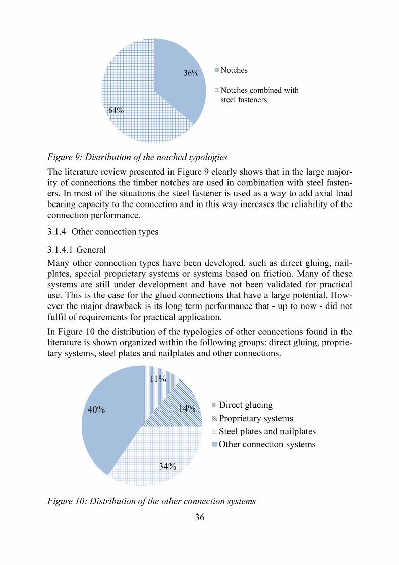
In Figure 9 the distribution of the typologies of notch configurations found in the literature is presented, organized within the following groups: notches, notches combined with steel fasteners.
36
Figure 9: Distribution of the notched typologies
The literature review presented in Figure 9 clearly shows that in the large major-ity of connections the timber notches are used in combination with steel fasten-ers. In most of the situations the steel fastener is used as a way to add axial load bearing capacity to the connection and in this way increases the reliability of the connection performance.
3.1.4 Other connection types
3.1.4.1 General Many other connection types have been developed, such as direct gluing, nail-plates, special proprietary systems or systems based on friction. Many of these systems are still under development and have not been validated for practical use. This is the case for the glued connections that have a large potential. How-ever the major drawback is its long term performance that - up to now - did not fulfil of requirements for practical application.
In Figure 10 the distribution of the typologies of other connections found in the literature is shown organized within the following groups: direct gluing, proprie-tary systems, steel plates and nailplates and other connections.
Figure 10: Distribution of the other connection systems
37
Figure 10 shows a large variability that can be found in these connection sys-tems. 40% cannot be assigned to any particular group. The glued systems do al-ready represent a significant proportion of the research studies available, result-ing from the large interest in the recent years. On the other hand, the proprietary systems show a small share in the number of studies, which is not representative of their use in practice. This is probably a consequence of the patent require-ments that do not promote or motivate the publication of the related research re-sults. Due to its innovative character further details are given for a number of such systems.
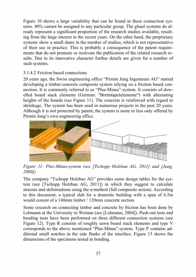
3.1.4.2 Friction based connections 20 years ago, the Swiss engineering office “Pirmin Jung Ingenieure AG” started developing a timber-concrete composite system relying on a friction based con-nection. It is commonly referred to as “Plus-Minus”-system. It consists of dow-elled board stack elements (German: "Brettstapelelemente") with alternating heights of the boards (see Figure 11). The concrete is reinforced with regard to shrinkage. The system has been used in numerous projects in the past 20 years. Although it is not protected by patent, the system is more or less only offered by Pirmin Jung’s own engineering office.
Figure 11: Plus-Minus-system (see [Tschopp Holzbau AG, 2011] and [Jung, 2000])
The company “Tschopp Holzbau AG” provides some design tables for the sys-tem (see [Tschopp Holzbau AG, 2011]) in which they suggest to calculate stresses and deformations using the n-method (full composite action). According to this document, a typical slab for a domestic building with a span of 6.5m would consist of a 140mm timber / 120mm concrete section.
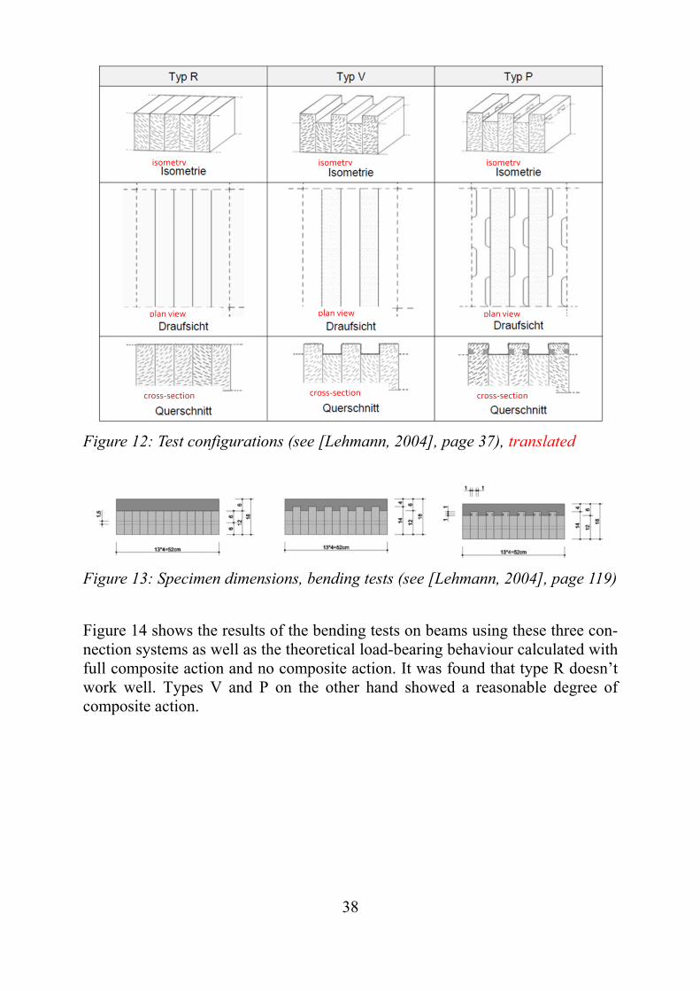
Some research on connecting timber and concrete by friction has been done by Lehmann at the University in Weimar (see [Lehmann, 2004]). Push-out tests and bending tests have been performed on three different connection systems (see Figure 12). Type R consists of roughly sawn board stack elements and type V corresponds to the above mentioned “Plus-Minus”-system. Type P contains ad-ditional small notches in the side flanks of the interface. Figure 13 shows the dimensions of the specimens tested in bending.
38
Figure 12: Test configurations (see [Lehmann, 2004], page 37), translated
Figure 13: Specimen dimensions, bending tests (see [Lehmann, 2004], page 119)
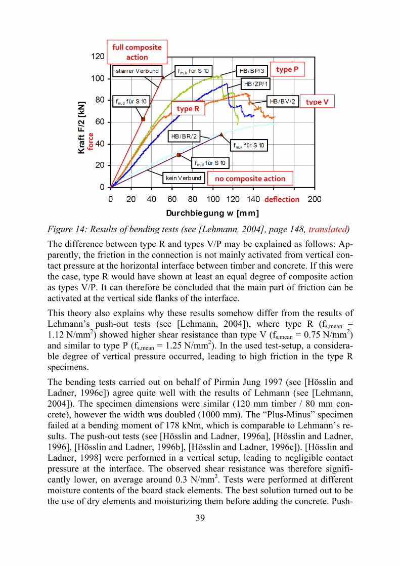
Figure 14 shows the results of the bending tests on beams using these three con-nection systems as well as the theoretical load-bearing behaviour calculated with full composite action and no composite action. It was found that type R doesn’t work well. Types V and P on the other hand showed a reasonable degree of composite action.
cross‐section
plan view plan view plan view
isometry isometry isometry
cross‐section cross‐section
39
Figure 14: Results of bending tests (see [Lehmann, 2004], page 148, translated)
The difference between type R and types V/P may be explained as follows: Ap-parently, the friction in the connection is not mainly activated from vertical con-tact pressure at the horizontal interface between timber and concrete. If this were the case, type R would have shown at least an equal degree of composite action as types V/P. It can therefore be concluded that the main part of friction can be activated at the vertical side flanks of the interface.
This theory also explains why these results somehow differ from the results of Lehmann’s push-out tests (see [Lehmann, 2004]), where type R (fs,mean = 1.12 N/mm2) showed higher shear resistance than type V (fs,mean = 0.75 N/mm2) and similar to type P (fs,mean = 1.25 N/mm2). In the used test-setup, a considera-ble degree of vertical pressure occurred, leading to high friction in the type R specimens.
The bending tests carried out on behalf of Pirmin Jung 1997 (see [Hösslin and Ladner, 1996c]) agree quite well with the results of Lehmann (see [Lehmann, 2004]). The specimen dimensions were similar (120 mm timber / 80 mm con-crete), however the width was doubled (1000 mm). The “Plus-Minus” specimen failed at a bending moment of 178 kNm, which is comparable to Lehmann’s re-sults. The push-out tests (see [Hösslin and Ladner, 1996a], [Hösslin and Ladner, 1996], [Hösslin and Ladner, 1996b], [Hösslin and Ladner, 1996c]). [Hösslin and Ladner, 1998] were performed in a vertical setup, leading to negligible contact pressure at the interface. The observed shear resistance was therefore signifi-cantly lower, on average around 0.3 N/mm2. Tests were performed at different moisture contents of the board stack elements. The best solution turned out to be the use of dry elements and moisturizing them before adding the concrete. Push-
type R type V
type P
no composite action
full composite action
deflection
force
40
out tests were performed both on specimens 28 days and 1 year after construc-tion. The latter specimens showed a 30 – 40 % lower shear resistance with re-spect to the specimens that were tested after 28 days (see [Hösslin and Ladner, 1998]). For this connection, investigations with regard to the fire safety have been carried out by Frangi (see [Frangi, 2001]). A fire resistance of 2 hours was observed experimentally.
The “Plus-Minus”-system has been successfully used in numerous projects in Switzerland in the past 20 years. However, the available fundamental research on this topic is not sufficient enough to serve as a basis for a future code. On the other hand, since many projects have shown that the Plus-Minus-system works, the consideration of friction should not explicitly be forbidden.
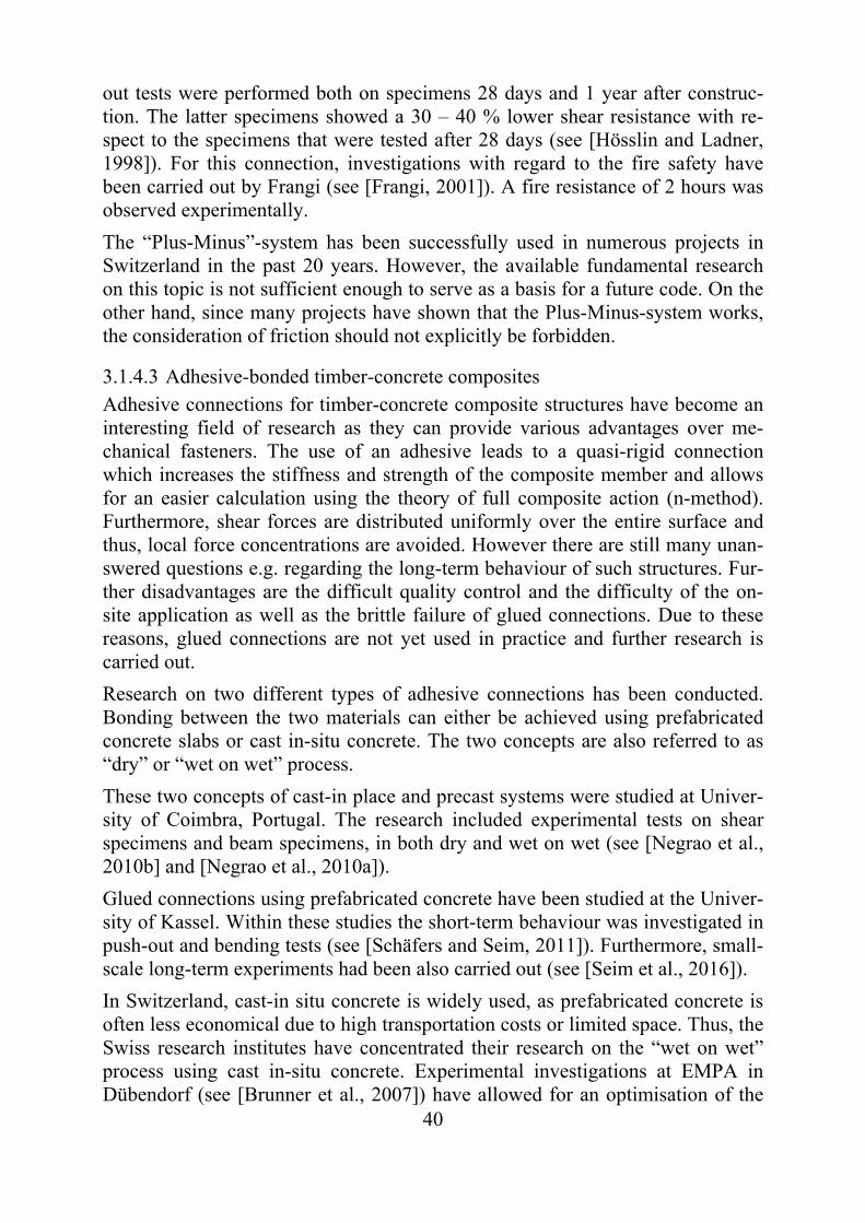
3.1.4.3 Adhesive-bonded timber-concrete composites Adhesive connections for timber-concrete composite structures have become an interesting field of research as they can provide various advantages over me-chanical fasteners. The use of an adhesive leads to a quasi-rigid connection which increases the stiffness and strength of the composite member and allows for an easier calculation using the theory of full composite action (n-method). Furthermore, shear forces are distributed uniformly over the entire surface and thus, local force concentrations are avoided. However there are still many unan-swered questions e.g. regarding the long-term behaviour of such structures. Fur-ther disadvantages are the difficult quality control and the difficulty of the on-site application as well as the brittle failure of glued connections. Due to these reasons, glued connections are not yet used in practice and further research is carried out.
Research on two different types of adhesive connections has been conducted. Bonding between the two materials can either be achieved using prefabricated concrete slabs or cast in-situ concrete. The two concepts are also referred to as “dry” or “wet on wet” process.
These two concepts of cast-in place and precast systems were studied at Univer-sity of Coimbra, Portugal. The research included experimental tests on shear specimens and beam specimens, in both dry and wet on wet (see [Negrao et al., 2010b] and [Negrao et al., 2010a]).
Glued connections using prefabricated concrete have been studied at the Univer-sity of Kassel. Within these studies the short-term behaviour was investigated in push-out and bending tests (see [Schäfers and Seim, 2011]). Furthermore, small-scale long-term experiments had been also carried out (see [Seim et al., 2016]).
In Switzerland, cast-in situ concrete is widely used, as prefabricated concrete is often less economical due to high transportation costs or limited space. Thus, the Swiss research institutes have concentrated their research on the “wet on wet” process using cast in-situ concrete. Experimental investigations at EMPA in Dübendorf (see [Brunner et al., 2007]) have allowed for an optimisation of the
41
production process. Nevertheless the danger of adhesive displacement during the pouring of concrete is still present. The performed bending tests showed promis-ing results with respect to stiffness and strength.
This research continues within a new project at the Chair of Wood Materials Science at ETH Zurich, using beech LVL. The wood surface is chemically mod-ified in order to improve the compatibility with the adhesive (similar to a bond-ing primer) and to prevent the beech boards from soaking up water from the fresh concrete (see [Kostica et al., 2018]). Push-out tests have been performed using three different glue types. Failure was either brittle at high loads (> 4 N/mm2) or fairly ductile at a lower load level (1 N/mm2), depending on the type of glue used. Both adhesive types might be interesting for future use in TCC structures.
Several research projects have demonstrated the potential of adhesive connec-tions in timber-concrete composite structures. To apply glued connections in practice, however, more research is necessary especially with respect to the long-term behaviour and also the quality control during production.
3.1.4.4 Concrete-type adhesives The connecting technology uses concrete-type adhesives and larger drill-holes or slots to overcome the uncertainness of the bond line quality in glued-in rods and the structural performance of miss-glued connections. The jointing system is suitable for pre-fabricated truss structures as well in structural rehabilitation of traditional flooring systems and slabs. Due to preparation on site, the CTA adapts exactly the joint surface, whatever it looks like.
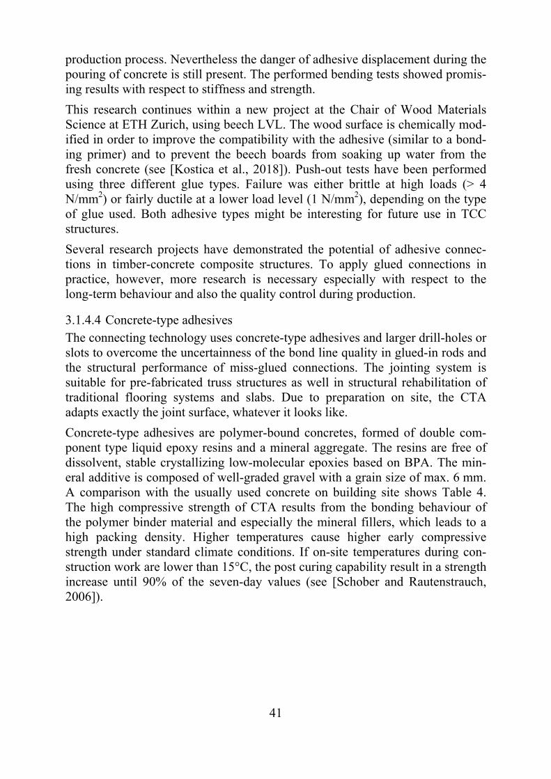
Concrete-type adhesives are polymer-bound concretes, formed of double com-ponent type liquid epoxy resins and a mineral aggregate. The resins are free of dissolvent, stable crystallizing low-molecular epoxies based on BPA. The min-eral additive is composed of well-graded gravel with a grain size of max. 6 mm. A comparison with the usually used concrete on building site shows Table 4. The high compressive strength of CTA results from the bonding behaviour of the polymer binder material and especially the mineral fillers, which leads to a high packing density. Higher temperatures cause higher early compressive strength under standard climate conditions. If on-site temperatures during con-struction work are lower than 15°C, the post curing capability result in a strength increase until 90% of the seven-day values (see [Schober and Rautenstrauch, 2006]).
42
Table 4: Comparison of used CTA with reinforced concrete following [EN 206-1].
Material property CTA1 RC C25/30 Ratio
Density 2.0 g/cm³ 2.4 g/cm³ 0.83
Tensile MOE 19,600 MPa 30,000 MPa 0.64
Bending strength 30 MPa 5.5 MPa 5.45
Compressive strength
110 MPa 30 MPa 3.37
1 curing under standard climate conditions 7d / 20°C / 65% RH
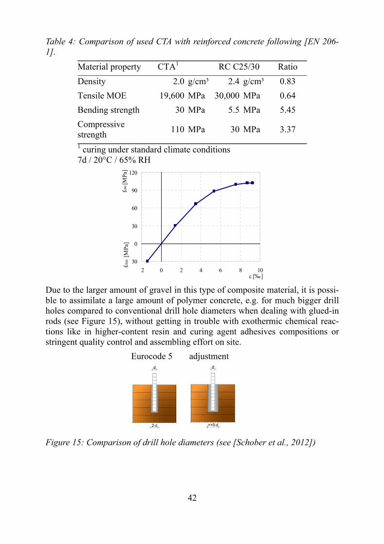
Due to the larger amount of gravel in this type of composite material, it is possi-ble to assimilate a large amount of polymer concrete, e.g. for much bigger drill holes compared to conventional drill hole diameters when dealing with glued-in rods (see Figure 15), without getting in trouble with exothermic chemical reac-tions like in higher-content resin and curing agent adhesives compositions or stringent quality control and assembling effort on site.
Eurocode 5
adjustment
Figure 15: Comparison of drill hole diameters (see [Schober et al., 2012])
-30
0
30
60
90
120
-2 0 2 4 6 8 10 [‰]
fcm [M
Pa]
fctm
[M
Pa]
43
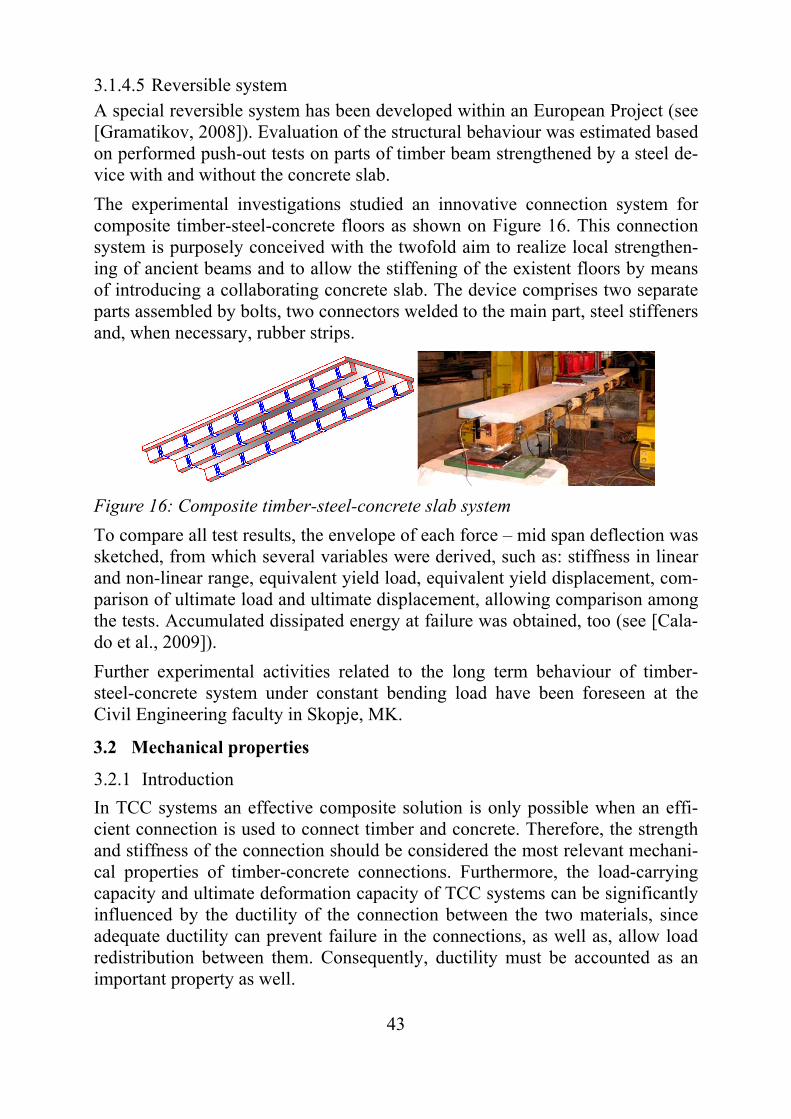
3.1.4.5 Reversible system A special reversible system has been developed within an European Project (see [Gramatikov, 2008]). Evaluation of the structural behaviour was estimated based on performed push-out tests on parts of timber beam strengthened by a steel de-vice with and without the concrete slab.
The experimental investigations studied an innovative connection system for composite timber-steel-concrete floors as shown on Figure 16. This connection system is purposely conceived with the twofold aim to realize local strengthen-ing of ancient beams and to allow the stiffening of the existent floors by means of introducing a collaborating concrete slab. The device comprises two separate parts assembled by bolts, two connectors welded to the main part, steel stiffeners and, when necessary, rubber strips.
Figure 16: Composite timber-steel-concrete slab system
To compare all test results, the envelope of each force – mid span deflection was sketched, from which several variables were derived, such as: stiffness in linear and non-linear range, equivalent yield load, equivalent yield displacement, com-parison of ultimate load and ultimate displacement, allowing comparison among the tests. Accumulated dissipated energy at failure was obtained, too (see [Cala-do et al., 2009]).
Further experimental activities related to the long term behaviour of timber-steel-concrete system under constant bending load have been foreseen at the Civil Engineering faculty in Skopje, MK.
3.2 Mechanical properties
3.2.1 Introduction
In TCC systems an effective composite solution is only possible when an effi-cient connection is used to connect timber and concrete. Therefore, the strength and stiffness of the connection should be considered the most relevant mechani-cal properties of timber-concrete connections. Furthermore, the load-carrying capacity and ultimate deformation capacity of TCC systems can be significantly influenced by the ductility of the connection between the two materials, since adequate ductility can prevent failure in the connections, as well as, allow load redistribution between them. Consequently, ductility must be accounted as an important property as well.
44
Generally, to estimate the mechanical properties of a timber-concrete connec-tion, experimental laboratory tests are carried out; seldom numerical models are used to predict the connection behaviour and its mechanical properties.
3.2.2 Stiffness
The stiffness of TCC systems governs the deformations at the interface. The lev-el of composite action achieved in the system depends directly on the defor-mation at the interface. Usually the stiffness of the connection is assumed as the connection slip modulus as defined in [EN 26891].
In TCC systems as indeterminate system, the stiffness of the connection influ-ences the bending stiffness and therefore the deformation, internal forces and stress distribution in the whole structure. For this reason the stiffness of TCC systems has an important influence in the verification of both, Serviceability Limit States and Ultimate Limit States.
As referred by [Ceccotti, 1995], the stiffness of a connection system can be as-sumed as a sort of classification index. The variability of the stiffness in timber-concrete connections can be seen as the main design parameter of each connec-tion type.
3.2.3 Strength
The strength of a TCC connection is the maximum shear load that can be trans-mitted at the interface between timber and concrete. It is usually assumed as the maximum load the connection can carry up to a maximum slip of 15 mm as de-fined in [EN 26891]
In any case it is important to note that the load appearing in the connection is dependent on its deformation and the connection load level is closely related to the connection stiffness.
3.2.4 Ductility
Timber-concrete connections with steel connectors usually do behave in a duc-tile manner whilst notched connections usually behave in a brittle manner. The behaviour of connections can vary between connections that are very stiff with low ductility, to those that are very flexible and ductile (see [Ceccotti, 2002]), depending on the type of connectors used and configuration of the connection. The use of more ductile connections can increase the load-carrying capacity of the composite system as well as its ultimate deformation capacity (see [Dias and Jorge, 2011]). Despite of that fact, [Ceccotti, 2002] indicates that the ductile be-haviour of a TCC system is not necessarily achieved just because connections exhibit a ductile behaviour. If the stiffness of the connection is greater than pre-dicted, timber may reach its rupture strength while connections are still respond-ing elastically. Consequently, the system will be much less ductile than antici-pated. [Van der Linden, 1999] gives an example based on numerical simulations
45
of how ductile types of connectors can be of great importance in timber-concrete composites.
3.3 Code Rules and Guidelines available
3.3.1 Introduction
In spite of the high interest raised for this structural system, its design was never complemented by an adequate regulatory framework. Indeed, some disperse rules/guidelines have been developed, but mostly to answer particular issues such as for example the design of bridges (see [Dias, 2016]). Nevertheless, in-formation related to the connections is often given in the available documents.
Five national/regional documents were identified:
Europe – Eurocode 5 (see [EN 1995-1-1] and [EN 1995-2]); Oceania – Australia and New Zealand design Guidelines (see [Gerber et
al., 2012]); USA – AASHO/AASTHO codes (see [AASHO, 1949] and [AASHTO,
1983]) Canada – Canadian Highway Bridge Design Code (see [CSA, 2006]); Brazil – Manual for the design of timber bridges (see [Junior et al.,
2006]).
3.3.2 Eurocode 5
In Eurocode 5 Part 1-1 “General – Common rules and rules for buildings” (see [EN 1995-1-1]) and Part 2 “Bridges” (see [EN 1995-2]), give some disperse clauses for the design of TCC systems. Additionally, other common clauses for timber structures are also often used for the TCC systems.
In terms of connections the following clauses are given, specifically and explic-itly for TCC systems:
Part 1-1 – Clause – 7.1 (3) Connection slip for concrete-to-timber connec-tions
Clause – 2.4.1 – Table 2.1 – Recommended partial factors for material properties;
Clause – 5.2 – Influence of the connection slip in composite action deck plate systems;
Clause – 5.3 (2) – Design of steel fasteners and grooved connections; Clause – 8.2 – Timber-concrete connections in Composite Systems.
Clause 7.1 indicates that the slip modulus of the timber-concrete connections can be obtained based on the models given for the timber connections multiplied by a factor 2. This approach implicitly assumes that the deformation on concrete side is negligible and the connections stiffness can be assumed to be double of
46
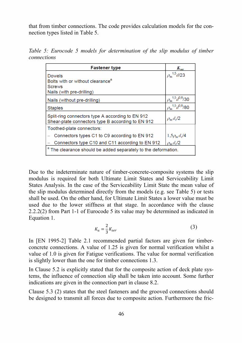
that from timber connections. The code provides calculation models for the con-nection types listed in Table 5.
Table 5: Eurocode 5 models for determination of the slip modulus of timber connections
Due to the indeterminate nature of timber-concrete-composite systems the slip modulus is required for both Ultimate Limit States and Serviceability Limit States Analysis. In the case of the Serviceability Limit State the mean value of the slip modulus determined directly from the models (e.g. see Table 5) or tests shall be used. On the other hand, for Ultimate Limit States a lower value must be used due to the lower stiffness at that stage. In accordance with the clause 2.2.2(2) from Part 1-1 of Eurocode 5 its value may be determined as indicated in Equation 1.
23
(3)
In [EN 1995-2] Table 2.1 recommended partial factors are given for timber-concrete connections. A value of 1.25 is given for normal verification whilst a value of 1.0 is given for Fatigue verifications. The value for normal verification is slightly lower than the one for timber connections 1.3.
In Clause 5.2 is explicitly stated that for the composite action of deck plate sys-tems, the influence of connection slip shall be taken into account. Some further indications are given in the connection part in clause 8.2.
Clause 5.3 (2) states that the steel fasteners and the grooved connections should be designed to transmit all forces due to composite action. Furthermore the fric-
47
tion and adhesion between wood and concrete should not be taken into account, unless a special investigation is carried out.
In Chapter 8 dealing with connections a number of indications are given for TCC that are transcribed below:
8.2.1(1) – The rope effect should not be used; 8.2.1(2) – In cases where there is an intermediate non-structural layer be-
tween the timber and the concrete (e.g. for formwork), the strength and stiffness parameters should be determined by a special analysis or by tests;
8.2.2 (1) – For grooved connections, the shear force should be taken by di-rect contact pressure between the wood and the concrete cast in the groove;
8.2.2 (2) It should be verified that the resistance of the concrete part and the timber part of the connection is sufficient;
8.2.2 (3) The concrete and timber parts shall be held together so that they cannot separate;
8.2.2 (4) The connection should be designed for a tensile force between the timber and the concrete equivalent to 10% of the shear load transmit-ted in the connection.
These indications are scarce and spread on the two Eurocode 5 parts mentioned (1-1 and 2). In most cases the application of TCC-connections according to [EN 1995-2] requires the use of other clauses originally meant for timber struc-tures.
3.3.3 Australia and New Zealand design Guidelines
[Gerber et al., 2012] presented a design guide to support the design of timber-concrete composite systems in Australia and New Zealand. This design guide is developed based on Eurocode 5 but adapted to comply with the Australian and New Zealand rules for timber structures. Some limitations apply to this proce-dure, due to the recognised uncertainty about some aspects of long term deflec-tion of TCC floors. Among these limitations, spans are limited to less than 8 m and two connection configurations prescribed in the document may be used (see [Crews and Gerber, 2010] and Figure 17).
The behaviour of the connections is assumed to be linear elastic for both Ulti-mate and Serviceability Limit States. The two connection configurations consist of notches combined with screws and are shown in Figure 17.
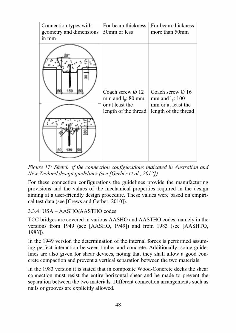
48
Connection types with geometry and dimensions in mm
For beam thickness 50mm or less
For beam thickness more than 50mm
Coach screw Ø 12 mm and lp: 80 mm or at least the length of the thread
Coach screw Ø 16 mm and lp: 100 mm or at least the length of the thread
Figure 17: Sketch of the connection configurations indicated in Australian and New Zealand design guidelines (see [Gerber et al., 2012])
For these connection configurations the guidelines provide the manufacturing provisions and the values of the mechanical properties required in the design aiming at a user-friendly design procedure. These values were based on empiri-cal test data (see [Crews and Gerber, 2010]).
3.3.4 USA – AASHO/AASTHO codes
TCC bridges are covered in various AASHO and AASTHO codes, namely in the versions from 1949 (see [AASHO, 1949]) and from 1983 (see [AASHTO, 1983]).
In the 1949 version the determination of the internal forces is performed assum-ing perfect interaction between timber and concrete. Additionally, some guide-lines are also given for shear devices, noting that they shall allow a good con-crete compaction and prevent a vertical separation between the two materials.
In the 1983 version it is stated that in composite Wood-Concrete decks the shear connection must resist the entire horizontal shear and be made to prevent the separation between the two materials. Different connection arrangements such as nails or grooves are explicitly allowed.
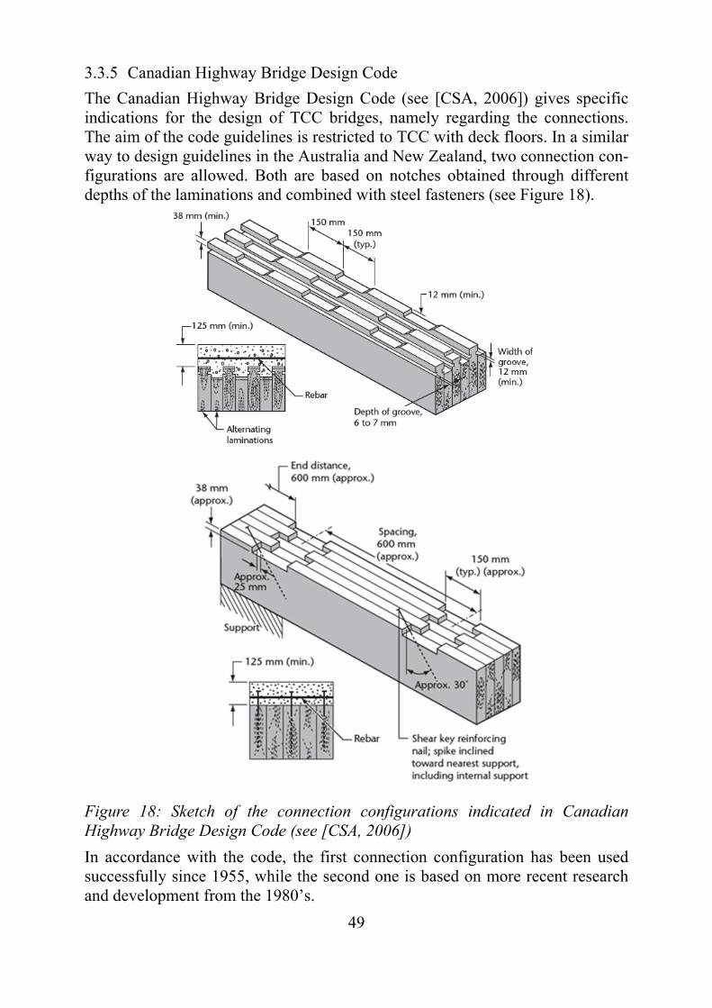
49
3.3.5 Canadian Highway Bridge Design Code
The Canadian Highway Bridge Design Code (see [CSA, 2006]) gives specific indications for the design of TCC bridges, namely regarding the connections. The aim of the code guidelines is restricted to TCC with deck floors. In a similar way to design guidelines in the Australia and New Zealand, two connection con-figurations are allowed. Both are based on notches obtained through different depths of the laminations and combined with steel fasteners (see Figure 18).
Figure 18: Sketch of the connection configurations indicated in Canadian Highway Bridge Design Code (see [CSA, 2006])
In accordance with the code, the first connection configuration has been used successfully since 1955, while the second one is based on more recent research and development from the 1980’s.
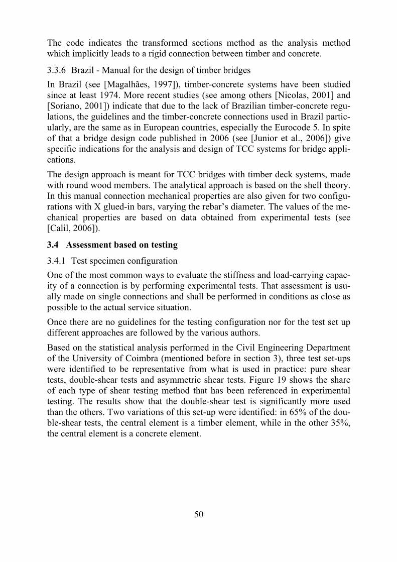
50
The code indicates the transformed sections method as the analysis method which implicitly leads to a rigid connection between timber and concrete.
3.3.6 Brazil - Manual for the design of timber bridges
In Brazil (see [Magalhães, 1997]), timber-concrete systems have been studied since at least 1974. More recent studies (see among others [Nicolas, 2001] and [Soriano, 2001]) indicate that due to the lack of Brazilian timber-concrete regu-lations, the guidelines and the timber-concrete connections used in Brazil partic-ularly, are the same as in European countries, especially the Eurocode 5. In spite of that a bridge design code published in 2006 (see [Junior et al., 2006]) give specific indications for the analysis and design of TCC systems for bridge appli-cations.
The design approach is meant for TCC bridges with timber deck systems, made with round wood members. The analytical approach is based on the shell theory. In this manual connection mechanical properties are also given for two configu-rations with X glued-in bars, varying the rebar’s diameter. The values of the me-chanical properties are based on data obtained from experimental tests (see [Calil, 2006]).
3.4 Assessment based on testing
3.4.1 Test specimen configuration
One of the most common ways to evaluate the stiffness and load-carrying capac-ity of a connection is by performing experimental tests. That assessment is usu-ally made on single connections and shall be performed in conditions as close as possible to the actual service situation.
Once there are no guidelines for the testing configuration nor for the test set up different approaches are followed by the various authors.
Based on the statistical analysis performed in the Civil Engineering Department of the University of Coimbra (mentioned before in section 3), three test set-ups were identified to be representative from what is used in practice: pure shear tests, double-shear tests and asymmetric shear tests. Figure 19 shows the share of each type of shear testing method that has been referenced in experimental testing. The results show that the double-shear test is significantly more used than the others. Two variations of this set-up were identified: in 65% of the dou-ble-shear tests, the central element is a timber element, while in the other 35%, the central element is a concrete element.
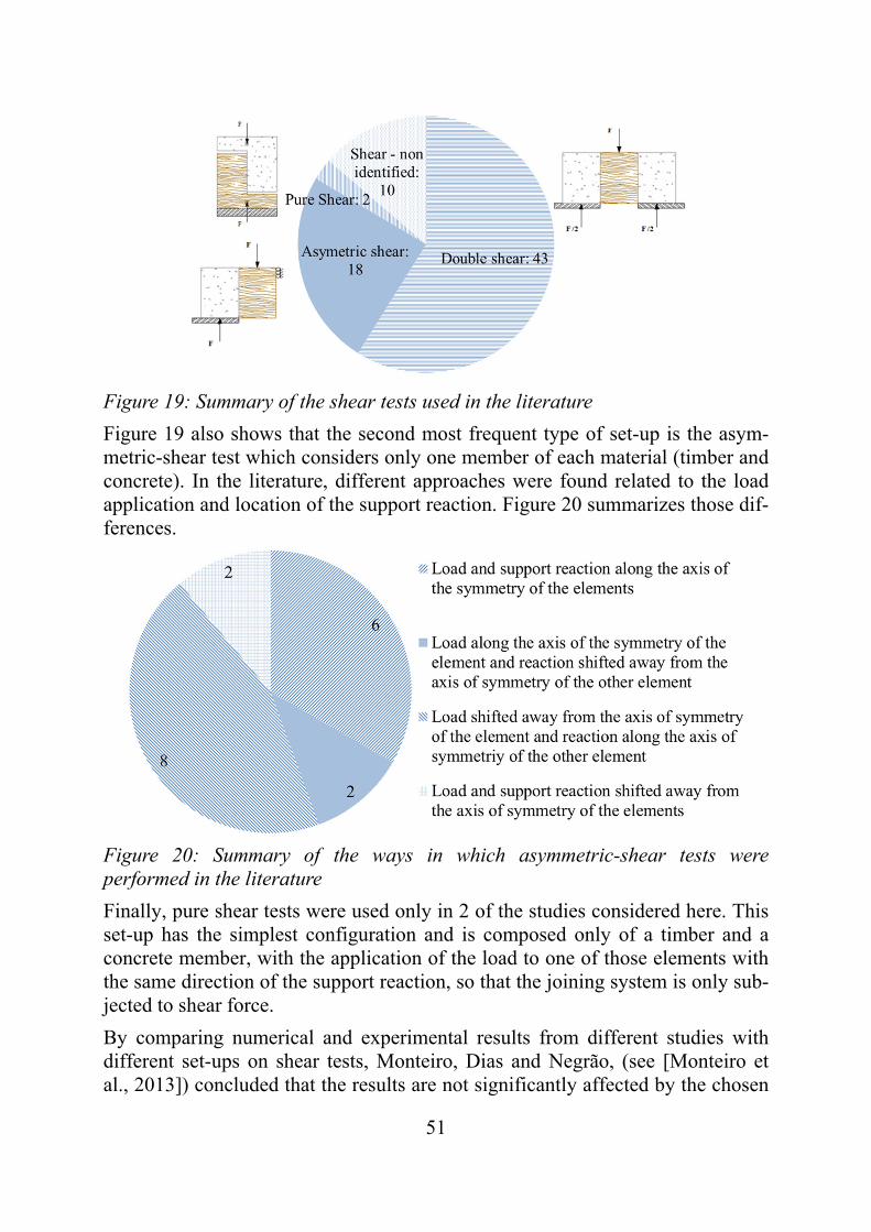
51
Figure 19: Summary of the shear tests used in the literature
Figure 19 also shows that the second most frequent type of set-up is the asym-metric-shear test which considers only one member of each material (timber and concrete). In the literature, different approaches were found related to the load application and location of the support reaction. Figure 20 summarizes those dif-ferences.
Figure 20: Summary of the ways in which asymmetric-shear tests were performed in the literature
Finally, pure shear tests were used only in 2 of the studies considered here. This set-up has the simplest configuration and is composed only of a timber and a concrete member, with the application of the load to one of those elements with the same direction of the support reaction, so that the joining system is only sub-jected to shear force.
By comparing numerical and experimental results from different studies with different set-ups on shear tests, Monteiro, Dias and Negrão, (see [Monteiro et al., 2013]) concluded that the results are not significantly affected by the chosen
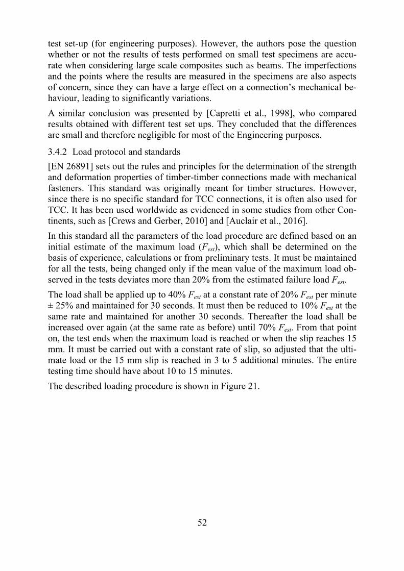
52
test set-up (for engineering purposes). However, the authors pose the question whether or not the results of tests performed on small test specimens are accu-rate when considering large scale composites such as beams. The imperfections and the points where the results are measured in the specimens are also aspects of concern, since they can have a large effect on a connection’s mechanical be-haviour, leading to significantly variations.
A similar conclusion was presented by [Capretti et al., 1998], who compared results obtained with different test set ups. They concluded that the differences are small and therefore negligible for most of the Engineering purposes.
3.4.2 Load protocol and standards
[EN 26891] sets out the rules and principles for the determination of the strength and deformation properties of timber-timber connections made with mechanical fasteners. This standard was originally meant for timber structures. However, since there is no specific standard for TCC connections, it is often also used for TCC. It has been used worldwide as evidenced in some studies from other Con-tinents, such as [Crews and Gerber, 2010] and [Auclair et al., 2016].
In this standard all the parameters of the load procedure are defined based on an initial estimate of the maximum load (Fest), which shall be determined on the basis of experience, calculations or from preliminary tests. It must be maintained for all the tests, being changed only if the mean value of the maximum load ob-served in the tests deviates more than 20% from the estimated failure load Fest.
The load shall be applied up to 40% Fest at a constant rate of 20% Fest per minute ± 25% and maintained for 30 seconds. It must then be reduced to 10% Fest at the same rate and maintained for another 30 seconds. Thereafter the load shall be increased over again (at the same rate as before) until 70% Fest. From that point on, the test ends when the maximum load is reached or when the slip reaches 15 mm. It must be carried out with a constant rate of slip, so adjusted that the ulti-mate load or the 15 mm slip is reached in 3 to 5 additional minutes. The entire testing time should have about 10 to 15 minutes.
The described loading procedure is shown in Figure 21.
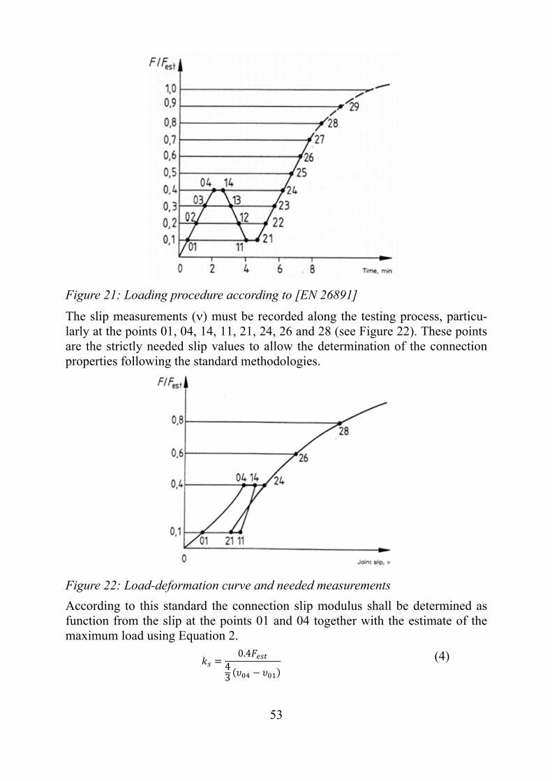
53
Figure 21: Loading procedure according to [EN 26891]
The slip measurements () must be recorded along the testing process, particu-larly at the points 01, 04, 14, 11, 21, 24, 26 and 28 (see Figure 22). These points are the strictly needed slip values to allow the determination of the connection properties following the standard methodologies.
Figure 22: Load-deformation curve and needed measurements
According to this standard the connection slip modulus shall be determined as function from the slip at the points 01 and 04 together with the estimate of the maximum load using Equation 2.
0.443
(4)
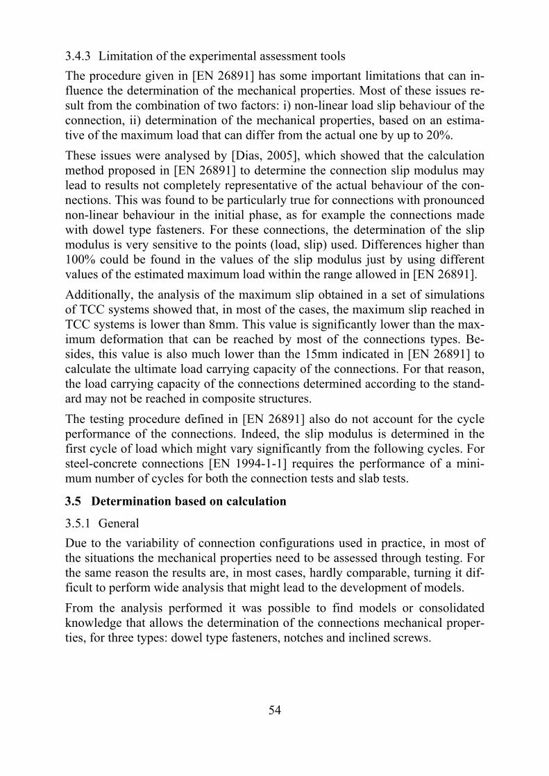
54
3.4.3 Limitation of the experimental assessment tools
The procedure given in [EN 26891] has some important limitations that can in-fluence the determination of the mechanical properties. Most of these issues re-sult from the combination of two factors: i) non-linear load slip behaviour of the connection, ii) determination of the mechanical properties, based on an estima-tive of the maximum load that can differ from the actual one by up to 20%.
These issues were analysed by [Dias, 2005], which showed that the calculation method proposed in [EN 26891] to determine the connection slip modulus may lead to results not completely representative of the actual behaviour of the con-nections. This was found to be particularly true for connections with pronounced non-linear behaviour in the initial phase, as for example the connections made with dowel type fasteners. For these connections, the determination of the slip modulus is very sensitive to the points (load, slip) used. Differences higher than 100% could be found in the values of the slip modulus just by using different values of the estimated maximum load within the range allowed in [EN 26891].
Additionally, the analysis of the maximum slip obtained in a set of simulations of TCC systems showed that, in most of the cases, the maximum slip reached in TCC systems is lower than 8mm. This value is significantly lower than the max-imum deformation that can be reached by most of the connections types. Be-sides, this value is also much lower than the 15mm indicated in [EN 26891] to calculate the ultimate load carrying capacity of the connections. For that reason, the load carrying capacity of the connections determined according to the stand-ard may not be reached in composite structures.
The testing procedure defined in [EN 26891] also do not account for the cycle performance of the connections. Indeed, the slip modulus is determined in the first cycle of load which might vary significantly from the following cycles. For steel-concrete connections [EN 1994-1-1] requires the performance of a mini-mum number of cycles for both the connection tests and slab tests.
3.5 Determination based on calculation
3.5.1 General
Due to the variability of connection configurations used in practice, in most of the situations the mechanical properties need to be assessed through testing. For the same reason the results are, in most cases, hardly comparable, turning it dif-ficult to perform wide analysis that might lead to the development of models.
From the analysis performed it was possible to find models or consolidated knowledge that allows the determination of the connections mechanical proper-ties, for three types: dowel type fasteners, notches and inclined screws.
55
3.5.2 Dowel-type fasteners
3.5.2.1 Load Carrying Capacity Most of the model proposals for the dowel type fasteners in timber concrete composite structures (see Figure 23) available in the bibliography were based on models available for timber-timber connections (see [Gelfi et al., 2002] and [Di-as et al., 2007]).
a.) before casting b.) example of a failure mode
Figure 23: Dowel type fasteners
[Dias et al., 2007] tried three approaches for the determination of the load carry-ing capacity of timber-concrete dowel type fasteners (see Figure 24), always based on the European Yield model indicated in [EN 1995-1-1]:
Timber-Timber connection – Ductile behaviour with yielding assumed for concrete
Steel-Timber connection – Rigid behaviour assumed for concrete Timber-Timber connection with gap – Brittle behaviour assumed for con-
crete
The results obtained with these three models were compared with experimental results. This analysis led to results that agree reasonably well with the values measured in the tests.
The model results, however, tend to underestimate the load carrying capacity of the connections, especially when high strength concretes are used.
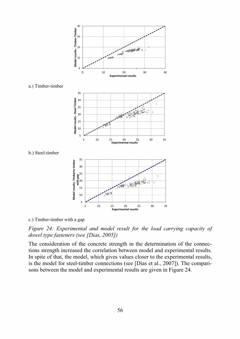
56
a.) Timber-timber
b.) Steel-timber
c.) Timber-timber with a gap
Figure 24: Experimental and model result for the load carrying capacity of dowel type fasteners (see [Dias, 2005])
The consideration of the concrete strength in the determination of the connec-tions strength increased the correlation between model and experimental results. In spite of that, the model, which gives values closer to the experimental results, is the model for steel-timber connections (see [Dias et al., 2007]). The compari-sons between the model and experimental results are given in Figure 24.
0
10
20
30
40
0 10 20 30 40Model results ‐Timber‐Tim
ber
Experimental results
5
10
15
20
25
30
35
5 10 15 20 25 30 35
Model results ‐Steel‐Timber
Experimental results
5
10
15
20
25
30
35
5 10 15 20 25 30 35
Model results‐Timberto tim
ber
with gap
Experimental results
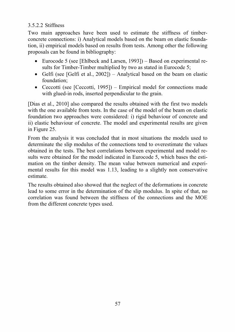
57
3.5.2.2 Stiffness Two main approaches have been used to estimate the stiffness of timber-concrete connections: i) Analytical models based on the beam on elastic founda-tion, ii) empirical models based on results from tests. Among other the following proposals can be found in bibliography:
Eurocode 5 (see [Ehlbeck and Larsen, 1993]) – Based on experimental re-sults for Timber-Timber multiplied by two as stated in Eurocode 5;
Gelfi (see [Gelfi et al., 2002]) – Analytical based on the beam on elastic foundation;
Ceccotti (see [Ceccotti, 1995]) – Empirical model for connections made with glued-in rods, inserted perpendicular to the grain.
[Dias et al., 2010] also compared the results obtained with the first two models with the one available from tests. In the case of the model of the beam on elastic foundation two approaches were considered: i) rigid behaviour of concrete and ii) elastic behaviour of concrete. The model and experimental results are given in Figure 25.
From the analysis it was concluded that in most situations the models used to determinate the slip modulus of the connections tend to overestimate the values obtained in the tests. The best correlations between experimental and model re-sults were obtained for the model indicated in Eurocode 5, which bases the esti-mation on the timber density. The mean value between numerical and experi-mental results for this model was 1.13, leading to a slightly non conservative estimate.
The results obtained also showed that the neglect of the deformations in concrete lead to some error in the determination of the slip modulus. In spite of that, no correlation was found between the stiffness of the connections and the MOE from the different concrete types used.
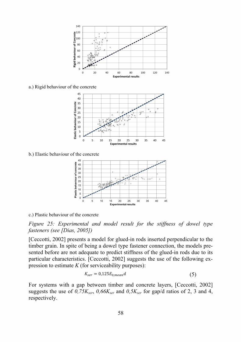
58
a.) Rigid behaviour of the concrete
b.) Elastic behaviour of the concrete
c.) Plastic behaviour of the concrete
Figure 25: Experimental and model result for the stiffness of dowel type fasteners (see [Dias, 2005])
[Ceccotti, 2002] presents a model for glued-in rods inserted perpendicular to the timber grain. In spite of being a dowel type fastener connection, the models pre-sented before are not adequate to predict stiffness of the glued-in rods due to its particular characteristics. [Ceccotti, 2002] suggests the use of the following ex-pression to estimate K (for serviceability purposes):
0,125 , (5)
For systems with a gap between timber and concrete layers, [Ceccotti, 2002] suggests the use of 0,75Kser, 0,66Kser and 0,5Kser for gap/d ratios of 2, 3 and 4, respectively.
0
20
40
60
80
100
120
140
0 20 40 60 80 100 120 140Rigid beh
aviour of Concrete
Experimental results
0
5
10
15
20
25
30
35
40
45
0 5 10 15 20 25 30 35 40 45
Elastic beh
aviour of Concrete
Experimental results
0
5
10
15
20
25
30
35
40
45
0 5 10 15 20 25 30 35 40 45
Pla
stic
be
hav
iou
r o
f co
ncr
ete
Experimental results
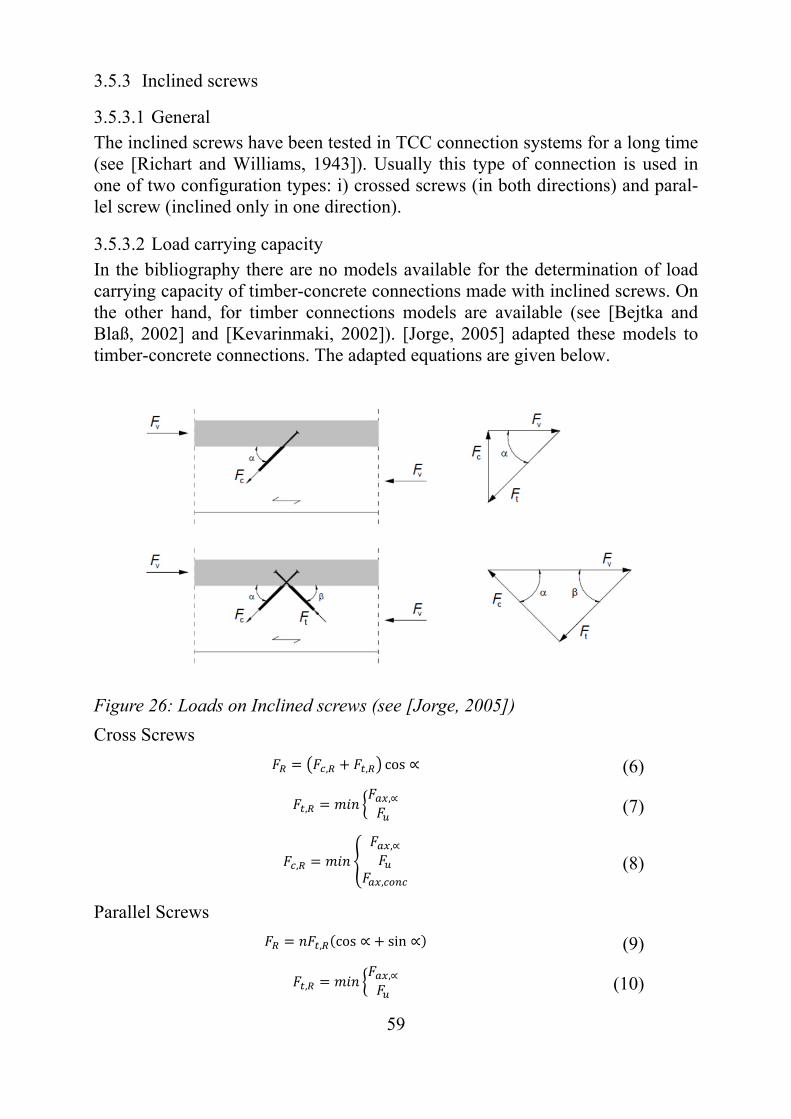
59
3.5.3 Inclined screws
3.5.3.1 General The inclined screws have been tested in TCC connection systems for a long time (see [Richart and Williams, 1943]). Usually this type of connection is used in one of two configuration types: i) crossed screws (in both directions) and paral-lel screw (inclined only in one direction).
3.5.3.2 Load carrying capacity In the bibliography there are no models available for the determination of load carrying capacity of timber-concrete connections made with inclined screws. On the other hand, for timber connections models are available (see [Bejtka and Blaß, 2002] and [Kevarinmaki, 2002]). [Jorge, 2005] adapted these models to timber-concrete connections. The adapted equations are given below.
Figure 26: Loads on Inclined screws (see [Jorge, 2005])
Cross Screws
, , cos ∝ (6)
,,∝ (7)
,
,∝
,
(8)
Parallel Screws
, cos ∝ sin ∝ (9)
,,∝ (10)
60
This model assumes that the withdrawal capacity is equal to the screw compres-sion capacity (see [Jorge, 2005]).
Results obtained with these models were compared with data available from tests. As a result, the prediction of the models is relatively in line with the exper-imental results. Furthermore, larger differences observed were on the conserva-tive side (see [Jorge, 2005]).
3.5.3.3 Stiffness There is no general model available in the bibliography to determine the stiff-ness properties of inclined screws. However in some ETAs the equations are given for the determination of the stiffness of this specific screw.
3.5.4 Notched Connections
3.5.4.1 General The analysis presented for notched connections is based on work performed within a FP 1402 STSM undertaken by Katrin Kudla from University of Stuttgart in University of Coimbra (see [Kudla, 2015]). This work is based on a detailed analysis of the studies available in the bibliography regarding timber-concrete notched connections. Since the work is also available in an independent publication from FP1402, only a brief resume, containing the main assumptions and recommendations will be given here.
The notched connections have been successfully used for almost 100 years, be-ing a simple and effective way to connect timber and concrete (see [Baldock and McCullough, 1941]). Its popularity is also motivated by the easy production with very simple tools to any desired configuration. On the other hand, this sim-plicity and flexibility complicate the standardization and the development of common rules and guidelines.
From the analysis of the research results available, Kudla proposes approaches for both, the load carrying capacity and stiffness determination. In both cases, a number of application restrictions, related to the notch configuration, are de-fined. These restrictions apply to: concrete, timber, notch depth, notch length, timber length in front of the notch and axial fastener diameter.

61
Figure 27: Geometrical parameters for a typical connection (see [Kudla, 2015])
Concrete:
• Minimum concrete strength class C 20/25 according to [EN 1992-1-1]
• Maximum grain size 16 mm
Timber:
• Glulam according to [EN 14080] (minimum GL 24h)
• Sawn softwood timber according to [EN 338] (minimum C 24)
Notch depth tv:
• tv ≥ 20mm for building applications
• tv ≥ 50mm for bridge applications
Notch length lN:
• lN ≥ 150mm
Timber length in front of the notch:
• lv ≥ 8 tv
Axial fastener diameter d:
• d ≥ 8mm
Additionally, a linear relationship between force and displacement is indicated for the design of these systems.
62
3.5.4.2 Load Carrying Capacity It is recommended that the load carrying capacity of the connections is deter-mined based on the failure modes that can be found in practice, namely:
• Longitudinal shear in timber
• Compression parallel to grain in timber
• Shear in concrete
• Compression in concrete
Further details on these failure modes it is suggested the use of the models avail-able in the Bibliography (see [Michelfelder, 2006], [Schönborn, 2006] and [Yeoh, 2010]).
3.5.4.3 Stiffness For notch depths between 2.0 and 3.0 cm a design value for the slip modulus of Kser = 1000 kN/mm per meter beam width is suggested. For notch depths deeper than 3.0 cm a design value Kser = 1500 kN/mm per meter beam width is consid-ered appropriate.
Additionally, it is mentioned that for a notched connection it is not suitable to distinguish between a slip modulus for serviceability and ultimate limit state. Load-displacement-curves from push-out tests and beam tests show a constant stiffness nearly until the load carrying capacity is reached. For this reason the assumption of Kser = Ku is suggested in the design of TCC systems with this connection type.
3.5.5 Connections with Interlayer
In many TCC systems an interlayer between timber and concrete is installed. The installation of this interlayer is almost always the case in the rehabilitation of timber floors but also when a lost formwork is used to cast the concrete mem-ber. This interlayer influences the mechanical performance of the connection in any composite system. Qualitatively this influence is relatively consensual and has been reported in several studies (see [Van der Linden, 1999], [Dias et al., 2004], [Jorge, 2005], [Dias et al., 2007] and [Dias et al., 2010]). On the other hand, the quantification of the influence varies significantly between the various studies available in the bibliography.
[EN 1995-2] – Bridges in section 8.2.1 recognises the specificities on TCC sys-tems with interlayer. It indicates for the cases with interlayer that the strength and stiffness parameters should be determined by a special analysis or by tests.
The results reported in a number of recent studies on both, the load carrying ca-pacity and stiffness of the connections, show a decrease of the mechanical prop-erties load carrying capacity and stiffness in connections with interlayer com-
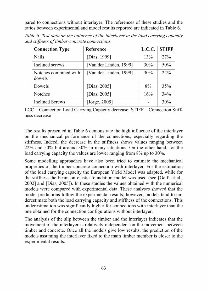
63
pared to connections without interlayer. The references of these studies and the ratios between experimental and model results reported are indicated in Table 6.
Table 6: Test data on the influence of the interlayer in the load carrying capacity and stiffness of timber-concrete connections
Connection Type Reference L.C.C. STIFF
Nails [Dias, 1999] 13% 27%
Inclined screws [Van der Linden, 1999] 30% 50%
Notches combined with dowels
[Van der Linden, 1999] 30% 22%
Dowels [Dias, 2005] 8% 35%
Notches [Dias, 2005] 16% 34%
Inclined Screws [Jorge, 2005] - 30%
LCC – Connection Load Carrying Capacity decrease; STIFF – Connection Stiff-ness decrease
The results presented in Table 6 demonstrate the high influence of the interlayer on the mechanical performance of the connections, especially regarding the stiffness. Indeed, the decrease in the stiffness shows values ranging between 22% and 50% but around 30% in many situations. On the other hand, for the load carrying capacity the values are lower ranging from 8% up to 30%.
Some modelling approaches have also been tried to estimate the mechanical properties of the timber-concrete connection with interlayer. For the estimation of the load carrying capacity the European Yield Model was adapted, while for the stiffness the beam on elastic foundation model was used (see [Gelfi et al., 2002] and [Dias, 2005]). In these studies the values obtained with the numerical models were compared with experimental data. These analyses showed that the model predictions follow the experimental results; however, models tend to un-derestimate both the load carrying capacity and stiffness of the connections. This underestimation was significantly higher for connections with interlayer than the one obtained for the connection configurations without interlayer.
The analysis of the slip between the timber and the interlayer indicates that the movement of the interlayer is relatively independent on the movement between timber and concrete. Once all the models give low results, the prediction of the models assuming the interlayer fixed to the main timber member is closer to the experimental results.
64
3.5.6 Load-Slip models
Usually a linear elastic approach is used in the analysis and design of TCC sys-tems. In these situations, two connection properties are required for the analysis: connection stiffness and the connection load carrying capacity (see [Dias et al., 2015]). Due to the non-linear behaviour of the connections these two properties may lead to significant errors in the analysis (see [Dias, 2012]). The improve-ment of the analysis is possible by the use of more sophisticated models such as for example the FEM non-linear models, which - on the other hand - require fur-ther connection mechanical properties, preferably the connection load-slip be-haviour. Unfortunately, the load-slip curves are usually not available for these types of connections. An approach to derive complete load-slip curves based solely on a limited number of mechanical properties was proposed by [Dias, 2005]. Later the analysis was extended to new types of connections and new mathematical models (see [Dias et al., 2015]). The types of connections consid-ered in these studies were:
Dowel-type fasteners;
Axially loaded fasteners;
Notches;
Notches combined with steel fasteners;
Nail plates;
Mathematical models were fitted to the experimental data. For the following model, parameters were delivered:
Foschi; [Foschi, 1974]
Goldberg-Richard-Abbott-Richard (GRAR); [Dias et al., 2015]
Yee-Melchers; [Dias et al., 2015]
Wu-Chen; [Dias et al., 2015]
Ollgaard-Slutter-Fisher (OSF). [Ollgaard et al., 1971]
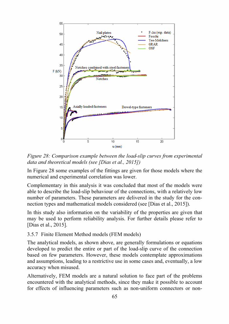
65
Figure 28: Comparison example between the load-slip curves from experimental data and theoretical models (see [Dias et al., 2015])
In Figure 28 some examples of the fittings are given for those models where the numerical and experimental correlation was lower.
Complementary in this analysis it was concluded that most of the models were able to describe the load-slip behaviour of the connections, with a relatively low number of parameters. These parameters are delivered in the study for the con-nection types and mathematical models considered (see [Dias et al., 2015]).
In this study also information on the variability of the properties are given that may be used to perform reliability analysis. For further details please refer to [Dias et al., 2015].
3.5.7 Finite Element Method models (FEM models)
The analytical models, as shown above, are generally formulations or equations developed to predict the entire or part of the load-slip curve of the connection based on few parameters. However, these models contemplate approximations and assumptions, leading to a restrictive use in some cases and, eventually, a low accuracy when misused.
Alternatively, FEM models are a natural solution to face part of the problems encountered with the analytical methods, since they make it possible to account for effects of influencing parameters such as non-uniform connectors or non-
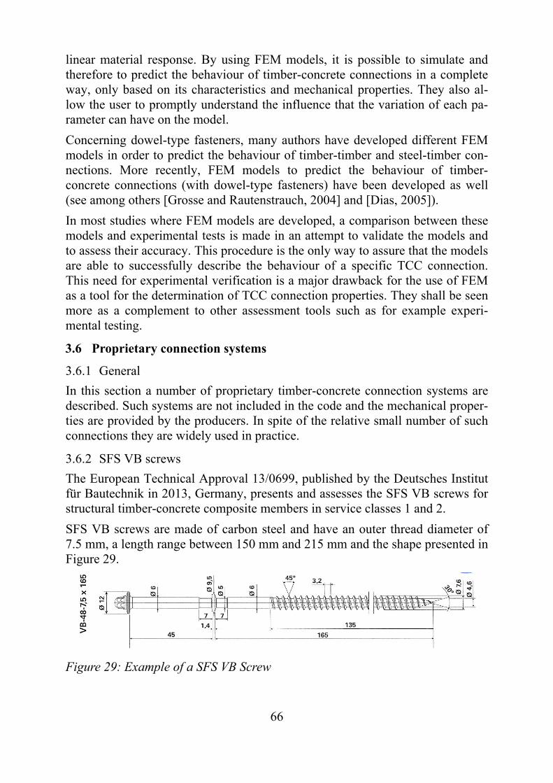
66
linear material response. By using FEM models, it is possible to simulate and therefore to predict the behaviour of timber-concrete connections in a complete way, only based on its characteristics and mechanical properties. They also al-low the user to promptly understand the influence that the variation of each pa-rameter can have on the model.
Concerning dowel-type fasteners, many authors have developed different FEM models in order to predict the behaviour of timber-timber and steel-timber con-nections. More recently, FEM models to predict the behaviour of timber-concrete connections (with dowel-type fasteners) have been developed as well (see among others [Grosse and Rautenstrauch, 2004] and [Dias, 2005]).
In most studies where FEM models are developed, a comparison between these models and experimental tests is made in an attempt to validate the models and to assess their accuracy. This procedure is the only way to assure that the models are able to successfully describe the behaviour of a specific TCC connection. This need for experimental verification is a major drawback for the use of FEM as a tool for the determination of TCC connection properties. They shall be seen more as a complement to other assessment tools such as for example experi-mental testing.
3.6 Proprietary connection systems
3.6.1 General
In this section a number of proprietary timber-concrete connection systems are described. Such systems are not included in the code and the mechanical proper-ties are provided by the producers. In spite of the relative small number of such connections they are widely used in practice.
3.6.2 SFS VB screws
The European Technical Approval 13/0699, published by the Deutsches Institut für Bautechnik in 2013, Germany, presents and assesses the SFS VB screws for structural timber-concrete composite members in service classes 1 and 2.
SFS VB screws are made of carbon steel and have an outer thread diameter of 7.5 mm, a length range between 150 mm and 215 mm and the shape presented in Figure 29.
Figure 29: Example of a SFS VB Screw
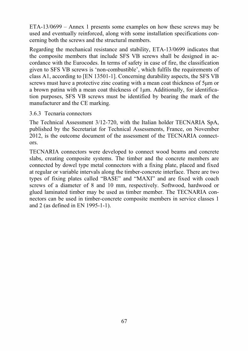
67
ETA-13/0699 – Annex 1 presents some examples on how these screws may be used and eventually reinforced, along with some installation specifications con-cerning both the screws and the structural members.
Regarding the mechanical resistance and stability, ETA-13/0699 indicates that the composite members that include SFS VB screws shall be designed in ac-cordance with the Eurocodes. In terms of safety in case of fire, the classification given to SFS VB screws is ‘non-combustible’, which fulfils the requirements of class A1, according to [EN 13501-1]. Concerning durability aspects, the SFS VB screws must have a protective zinc coating with a mean coat thickness of 5μm or a brown patina with a mean coat thickness of 1μm. Additionally, for identifica-tion purposes, SFS VB screws must be identified by bearing the mark of the manufacturer and the CE marking.
3.6.3 Tecnaria connectors
The Technical Assessment 3/12-720, with the Italian holder TECNARIA SpA, published by the Secretariat for Technical Assessments, France, on November 2012, is the outcome document of the assessment of the TECNARIA connect-ors.
TECNARIA connectors were developed to connect wood beams and concrete slabs, creating composite systems. The timber and the concrete members are connected by dowel type metal connectors with a fixing plate, placed and fixed at regular or variable intervals along the timber-concrete interface. There are two types of fixing plates called “BASE” and “MAXI” and are fixed with coach screws of a diameter of 8 and 10 mm, respectively. Softwood, hardwood or glued laminated timber may be used as timber member. The TECNARIA con-nectors can be used in timber-concrete composite members in service classes 1 and 2 (as defined in EN 1995-1-1).
68
Figure 30: Example of a TECNARIA connector
The section 2.3 of the TA 3/12-720 sets out the Special Technical Specifications that will assure the stability of the TECNARIA composite timber-concrete sys-tems throughout the establishment of design, manufacture, implementation and use principals, all in accordance with the Eurocodes.
As design and calculation conditions, the calculation method presented in TA 3/12-720 – Annex 1 must be followed, where different applications and types of connectors are considered and a design guide is provided, contemplating all phases needed for a correct design of the composite system with TECNARIA connectors. All the design process must be done using the values given in TA 3/12-720 – Annex 2, when applicable.
3.6.4 ASSY plus VG screws
The European Technical Approval 13/0029 (see [ETA 13/0029]) presents and assesses the ASSY plus VG screws for structural timber-concrete composite members in service classes 1 and 2 (as defined in [EN 1995-1-1]).
The diameter of the ASSY plus VG screws is either 8 mm or 10 mm and the length ranges between 150 mm and 180 mm. The shape and tolerances are given in ETA-13/0029 – Annex 3.
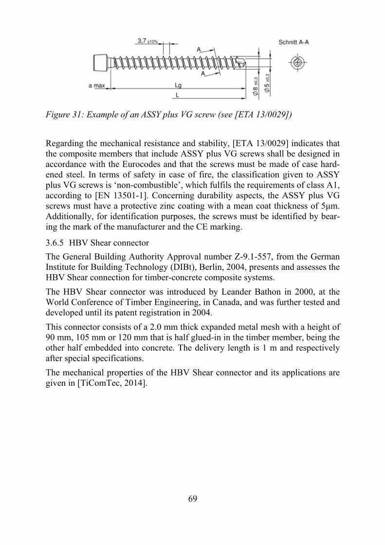
69
Figure 31: Example of an ASSY plus VG screw (see [ETA 13/0029])
Regarding the mechanical resistance and stability, [ETA 13/0029] indicates that the composite members that include ASSY plus VG screws shall be designed in accordance with the Eurocodes and that the screws must be made of case hard-ened steel. In terms of safety in case of fire, the classification given to ASSY plus VG screws is ‘non-combustible’, which fulfils the requirements of class A1, according to [EN 13501-1]. Concerning durability aspects, the ASSY plus VG screws must have a protective zinc coating with a mean coat thickness of 5μm. Additionally, for identification purposes, the screws must be identified by bear-ing the mark of the manufacturer and the CE marking.
3.6.5 HBV Shear connector
The General Building Authority Approval number Z-9.1-557, from the German Institute for Building Technology (DIBt), Berlin, 2004, presents and assesses the HBV Shear connection for timber-concrete composite systems.
The HBV Shear connector was introduced by Leander Bathon in 2000, at the World Conference of Timber Engineering, in Canada, and was further tested and developed until its patent registration in 2004.
This connector consists of a 2.0 mm thick expanded metal mesh with a height of 90 mm, 105 mm or 120 mm that is half glued-in in the timber member, being the other half embedded into concrete. The delivery length is 1 m and respectively after special specifications.
The mechanical properties of the HBV Shear connector and its applications are given in [TiComTec, 2014].
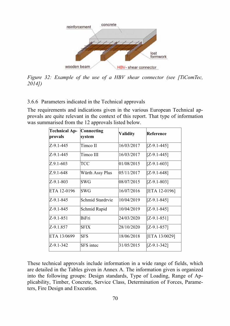
70
Figure 32: Example of the use of a HBV shear connector (see [TiComTec, 2014])
3.6.6 Parameters indicated in the Technical approvals
The requirements and indications given in the various European Technical ap-provals are quite relevant in the context of this report. That type of information was summarised from the 12 approvals listed below.
Technical Ap-provals
Connecting system
Validity Reference
Z-9.1-445 Timco II 16/03/2017 [Z-9.1-445]
Z-9.1-445 Timco III 16/03/2017 [Z-9.1-445]
Z.9.1-603 TCC 01/08/2015 [Z-9.1-603]
Z.9.1-648 Würth Assy Plus 05/11/2017 [Z-9.1-648]
Z-9.1-803 SWG 08/07/2015 [Z-9.1-803]
ETA 12-0196 SWG 16/07/2016 [ETA 12-0196]
Z-9.1-845 Schmid Stardrvie 10/04/2019 [Z-9.1-845]
Z-9.1-845 Schmid Rapid 10/04/2019 [Z-9.1-845]
Z-9.1-851 BiFri 24/03/2020 [Z-9.1-851]
Z-9.1.857 SFIX 28/10/2020 [Z-9.1-857]
ETA 13/0699 SFS 18/06/2018 [ETA 13/0029]
Z-9.1-342 SFS intec 31/05/2015 [Z-9.1-342]
These technical approvals include information in a wide range of fields, which are detailed in the Tables given in Annex A. The information given is organized into the following groups: Design standards, Type of Loading, Range of Ap-plicability, Timber, Concrete, Service Class, Determination of Forces, Parame-ters, Fire Design and Execution.
71
4. Evaluation of the forces
4.1 Preface
One essential part of the structural design is the determination of forces. With these forces the stresses are evaluated and the utilization of the system can be determined.
The way to determine the internal forces is one decision in the design process. The decision concerning the method chosen has to be made by the structural en-gineer. It is often influenced by the preferences and the practical experience of the designer. In order to allow for this freedom for the decision of the method within the standards, only boundary conditions and requirements can be given therein. In the following some of these boundary conditions and requirements are summarized.
4.2 Influences on the determination of the internal forces
In order to minimize the differences between the evaluated and the “real” stress-es in a structure, several parameters have to be considered in the design of com-posite systems (see among others [Aicher, 1987], [Baldock and McCullough, 1941], [Blaß et al., 1996], [Blaß et al., 1995]). The main influences on the inter-nal forces in a composite system are
Bending and normal stiffness of the composite elements, e.g. considera-tion of different Modulus of Elasticities and different cross sectional di-mensions
Behaviour of the joint between the components of the composite cross section
Inelastic strains due to temperature variation and/or shrinkage and swell-ing of the components of the composite cross sections
Long term behaviour of the components Non-linear behaviour e.g. caused by cracks or yielding of the material
All these influences have to be considered in the determination of forces. How-ever these boundaries can be organised into following subtopics:
Determination of the internal forces in the short-term for composite sys-tems taking into account the different material properties, the different cross sectional dimensions and the flexibility of the joint
Determination of the internal forces in the long-term Consideration of the material behaviour
72
4.3 Determination of forces in the short term
4.3.1 Consideration of the flexibility of the joint and the different cross section properties
In a composite system, external forces are distributed between the components of the composite cross section. In a composite cross section with 2 cross sec-tions, the equilibrium of forces is defined by the following equation:
⋅ (11)
where External bending moment
Bending moment in cross section 1
Bending moment in cross section 2
Normal force in both cross section
Distance between the centroids of both cross sections (=inner lever arm)
In principle, the system is statically undetermined, since neither the normal force nor the bending moment can be determined directly. In order to determine the forces in each component, the strains and curvature in the cross section are used, leading to following equations
Curvature in the single cross section: Assuming uplift between the single cross sections does not appear, the course of the deformation of the com-posite elements is equal. Since the curvature is the second derivation of the deformation, the curvature of the single cross section is identical:
(12)
Since the bending moment in a cross section depends on the stiffness and the curvature, the bending moment depends on
⋅ ⋅ (13)
Strain in the centroid: In principle, the strain in the centroid can be deter-mined by
⋅ (14)
However the normal force in the cross sections results in a slip in the joint due to the flexibility of the connection, which results in a reduced strain in the centroid. This reduced strain can be determined according to EC5 An-nex B by
(15)
Therefore the normal force in the cross section is determined by
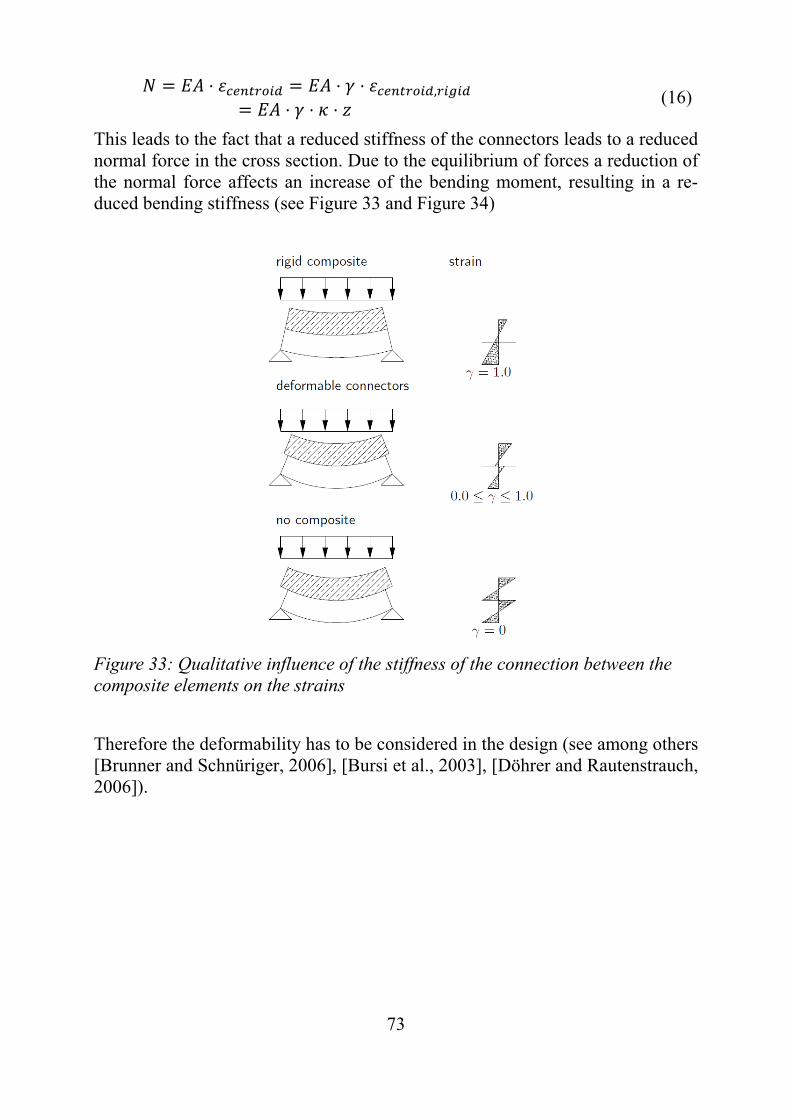
73
⋅ ⋅ ⋅ ,
⋅ ⋅ ⋅ (16)
This leads to the fact that a reduced stiffness of the connectors leads to a reduced normal force in the cross section. Due to the equilibrium of forces a reduction of the normal force affects an increase of the bending moment, resulting in a re-duced bending stiffness (see Figure 33 and Figure 34)
Figure 33: Qualitative influence of the stiffness of the connection between the composite elements on the strains
Therefore the deformability has to be considered in the design (see among others [Brunner and Schnüriger, 2006], [Bursi et al., 2003], [Döhrer and Rautenstrauch, 2006]).
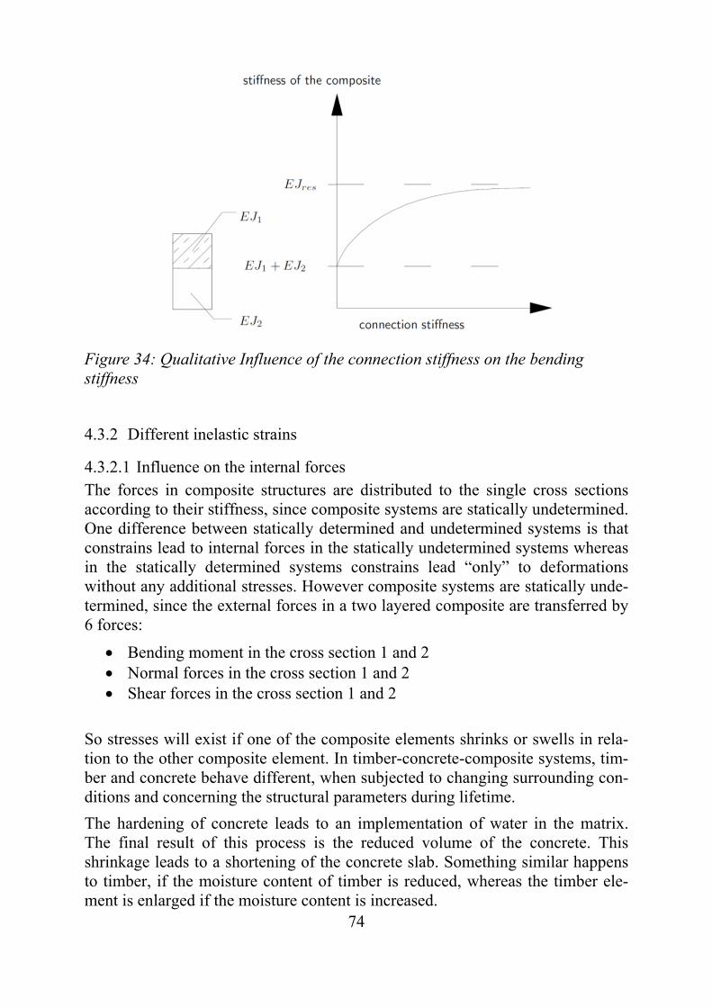
74
Figure 34: Qualitative Influence of the connection stiffness on the bending stiffness
4.3.2 Different inelastic strains
4.3.2.1 Influence on the internal forces The forces in composite structures are distributed to the single cross sections according to their stiffness, since composite systems are statically undetermined. One difference between statically determined and undetermined systems is that constrains lead to internal forces in the statically undetermined systems whereas in the statically determined systems constrains lead “only” to deformations without any additional stresses. However composite systems are statically unde-termined, since the external forces in a two layered composite are transferred by 6 forces:
Bending moment in the cross section 1 and 2 Normal forces in the cross section 1 and 2 Shear forces in the cross section 1 and 2
So stresses will exist if one of the composite elements shrinks or swells in rela-tion to the other composite element. In timber-concrete-composite systems, tim-ber and concrete behave different, when subjected to changing surrounding con-ditions and concerning the structural parameters during lifetime.
The hardening of concrete leads to an implementation of water in the matrix. The final result of this process is the reduced volume of the concrete. This shrinkage leads to a shortening of the concrete slab. Something similar happens to timber, if the moisture content of timber is reduced, whereas the timber ele-ment is enlarged if the moisture content is increased.
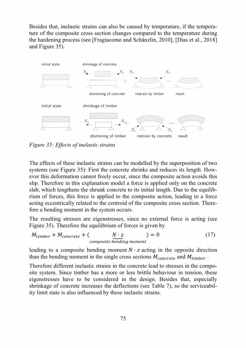
75
Besides that, inelastic strains can also be caused by temperature, if the tempera-ture of the composite cross section changes compared to the temperature during the hardening process (see [Fragiacomo and Schänzlin, 2010], [Dias et al., 2018] and Figure 35).
Figure 35: Effects of inelastic strains
The effects of these inelastic strains can be modelled by the superposition of two systems (see Figure 35): First the concrete shrinks and reduces its length. How-ever this deformation cannot freely occur, since the composite action avoids this slip. Therefore in this explanation model a force is applied only on the concrete slab, which lengthens the shrunk concrete to its initial length. Due to the equilib-rium of forces, this force is applied to the composite action, leading to a force acting eccentrically related to the centroid of the composite cross section. There-fore a bending moment in the system occurs.
The resulting stresses are eigenstresses, since no external force is acting (see Figure 35). Therefore the equilibrium of forces is given by
⋅
0 (17)
leading to a composite bending moment ⋅ acting in the opposite direction than the bending moment in the single cross sections and .
Therefore different inelastic strains in the concrete lead to stresses in the compo-site system. Since timber has a more or less brittle behaviour in tension, these eigenstresses have to be considered in the design. Besides that, especially shrinkage of concrete increases the deflections (see Table 7), so the serviceabil-ity limit state is also influenced by these inelastic strains.
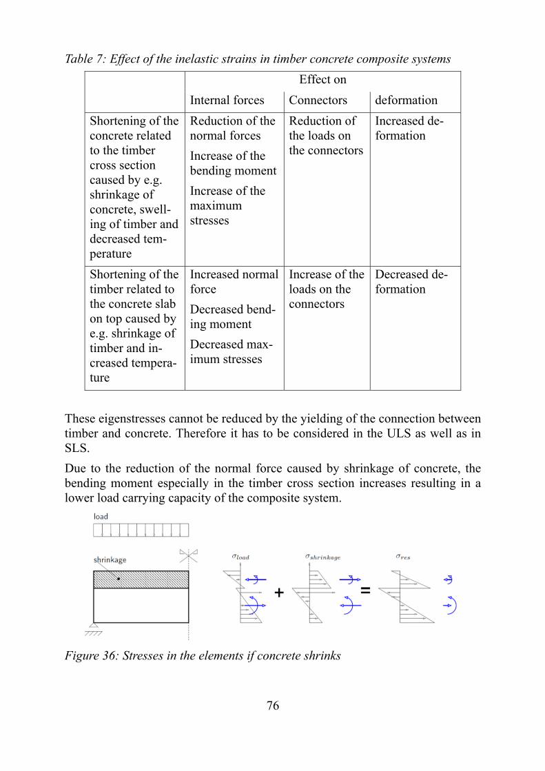
76
Table 7: Effect of the inelastic strains in timber concrete composite systems
Effect on
Internal forces Connectors deformation
Shortening of the concrete related to the timber cross section caused by e.g. shrinkage of concrete, swell-ing of timber and decreased tem-perature
Reduction of the normal forces
Increase of the bending moment
Increase of the maximum stresses
Reduction of the loads on the connectors
Increased de-formation
Shortening of the timber related to the concrete slab on top caused by e.g. shrinkage of timber and in-creased tempera-ture
Increased normal force
Decreased bend-ing moment
Decreased max-imum stresses
Increase of the loads on the connectors
Decreased de-formation
These eigenstresses cannot be reduced by the yielding of the connection between timber and concrete. Therefore it has to be considered in the ULS as well as in SLS.
Due to the reduction of the normal force caused by shrinkage of concrete, the bending moment especially in the timber cross section increases resulting in a lower load carrying capacity of the composite system.
Figure 36: Stresses in the elements if concrete shrinks
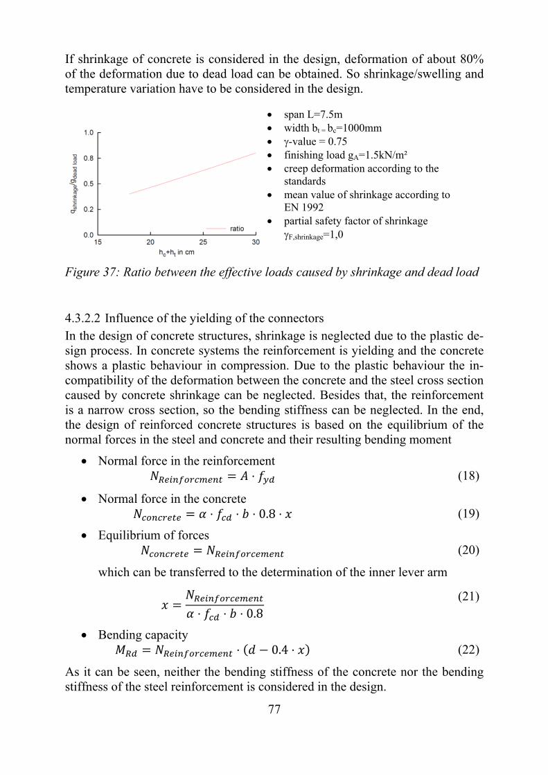
77
If shrinkage of concrete is considered in the design, deformation of about 80% of the deformation due to dead load can be obtained. So shrinkage/swelling and temperature variation have to be considered in the design.
Figure 37: Ratio between the effective loads caused by shrinkage and dead load
4.3.2.2 Influence of the yielding of the connectors In the design of concrete structures, shrinkage is neglected due to the plastic de-sign process. In concrete systems the reinforcement is yielding and the concrete shows a plastic behaviour in compression. Due to the plastic behaviour the in-compatibility of the deformation between the concrete and the steel cross section caused by concrete shrinkage can be neglected. Besides that, the reinforcement is a narrow cross section, so the bending stiffness can be neglected. In the end, the design of reinforced concrete structures is based on the equilibrium of the normal forces in the steel and concrete and their resulting bending moment
Normal force in the reinforcement ⋅ (18)
Normal force in the concrete ⋅ ⋅ ⋅ 0.8 ⋅ (19)
Equilibrium of forces (20)
which can be transferred to the determination of the inner lever arm
⋅ ⋅ ⋅ 0.8
(21)
Bending capacity ⋅ 0.4 ⋅ (22)
As it can be seen, neither the bending stiffness of the concrete nor the bending stiffness of the steel reinforcement is considered in the design.
span L=7.5m width bt = bc=1000mm -value = 0.75 finishing load gA=1.5kN/m² creep deformation according to the
standards mean value of shrinkage according to
EN 1992 partial safety factor of shrinkage
F,shrinkage=1,0
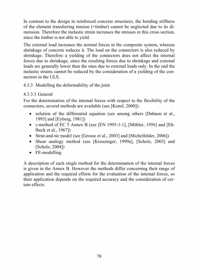
78
In contrast to the design in reinforced concrete structures, the bending stiffness of the element transferring tension (=timber) cannot be neglected due to its di-mension. Therefore the inelastic strain increases the stresses in this cross section, since the timber is not able to yield.
The external load increases the normal forces in the composite system, whereas shrinkage of concrete reduces it. The load on the connectors is also reduced by shrinkage. Therefore a yielding of the connectors does not affect the internal forces due to shrinkage, since the resulting forces due to shrinkage and external loads are generally lower than the ones due to external loads only. In the end the inelastic strains cannot be reduced by the consideration of a yielding of the con-nectors in the ULS.
4.3.3 Modelling the deformability of the joint
4.3.3.1 General For the determination of the internal forces with respect to the flexibility of the connectors, several methods are available (see [Kenel, 2000]):
solution of the differential equation (see among others [Dabaon et al., 1993] and [Eyberg, 1981])
-method of EC 5 Annex B (see [EN 1995-1-1], [Möhler, 1956] and [Eh-lbeck et al., 1967])
Strut-and-tie model (see [Grosse et al., 2003] and [Michelfelder, 2006]) Shear analogy method (see [Kreuzinger, 1999a], [Scholz, 2003] and
[Scholz, 2004]) FE-modelling
A description of each single method for the determination of the internal forces is given in the Annex B. However the methods differ concerning their range of application and the required efforts for the evaluation of the internal forces, so their application depends on the required accuracy and the consideration of cer-tain effects.
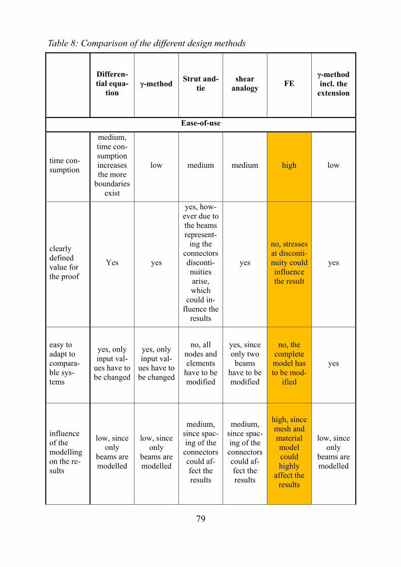
79
Table 8: Comparison of the different design methods
Differen-tial equa-
tion -method
Strut and-tie
shear analogy
FE -method incl. the
extension
Ease-of-use
time con-sumption
medium, time con-sumption increases the more
boundaries exist
low medium medium high low
clearly defined value for the proof
Yes yes
yes, how-ever due to the beams represent-
ing the connectors disconti-nuities arise, which
could in-fluence the
results
yes
no, stresses at disconti-nuity could influence the result
yes
easy to adapt to compara-ble sys-tems
yes, only input val-
ues have to be changed
yes, only input val-
ues have to be changed
no, all nodes and elements
have to be modified
yes, since only two beams
have to be modified
no, the complete model has to be mod-
ified
yes
influence of the modelling on the re-sults
low, since only
beams are modelled
low, since only
beams are modelled
medium, since spac-ing of the connectors could af-fect the results
medium, since spac-ing of the connectors could af-fect the results
high, since mesh and material model could highly
affect the results
low, since only
beams are modelled
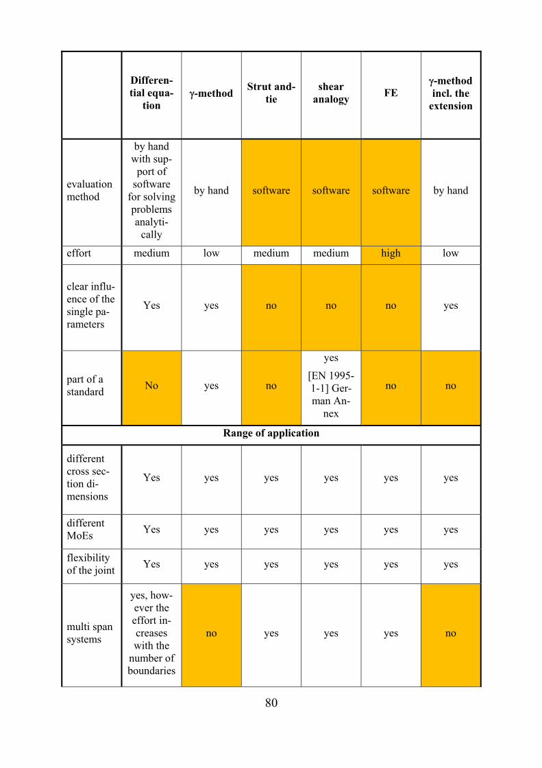
80
Differen-tial equa-
tion -method
Strut and-tie
shear analogy
FE -method incl. the
extension
evaluation method
by hand with sup-
port of software
for solving problems analyti-
cally
by hand software software software by hand
effort medium low medium medium high low
clear influ-ence of the single pa-rameters
Yes yes no no no yes
part of a standard
No yes no
yes
[EN 1995-1-1] Ger-man An-
nex
no no
Range of application
different cross sec-tion di-mensions
Yes yes yes yes yes yes
different MoEs
Yes yes yes yes yes yes
flexibility of the joint
Yes yes yes yes yes yes
multi span systems
yes, how-ever the effort in-creases with the
number of boundaries
no yes yes yes no
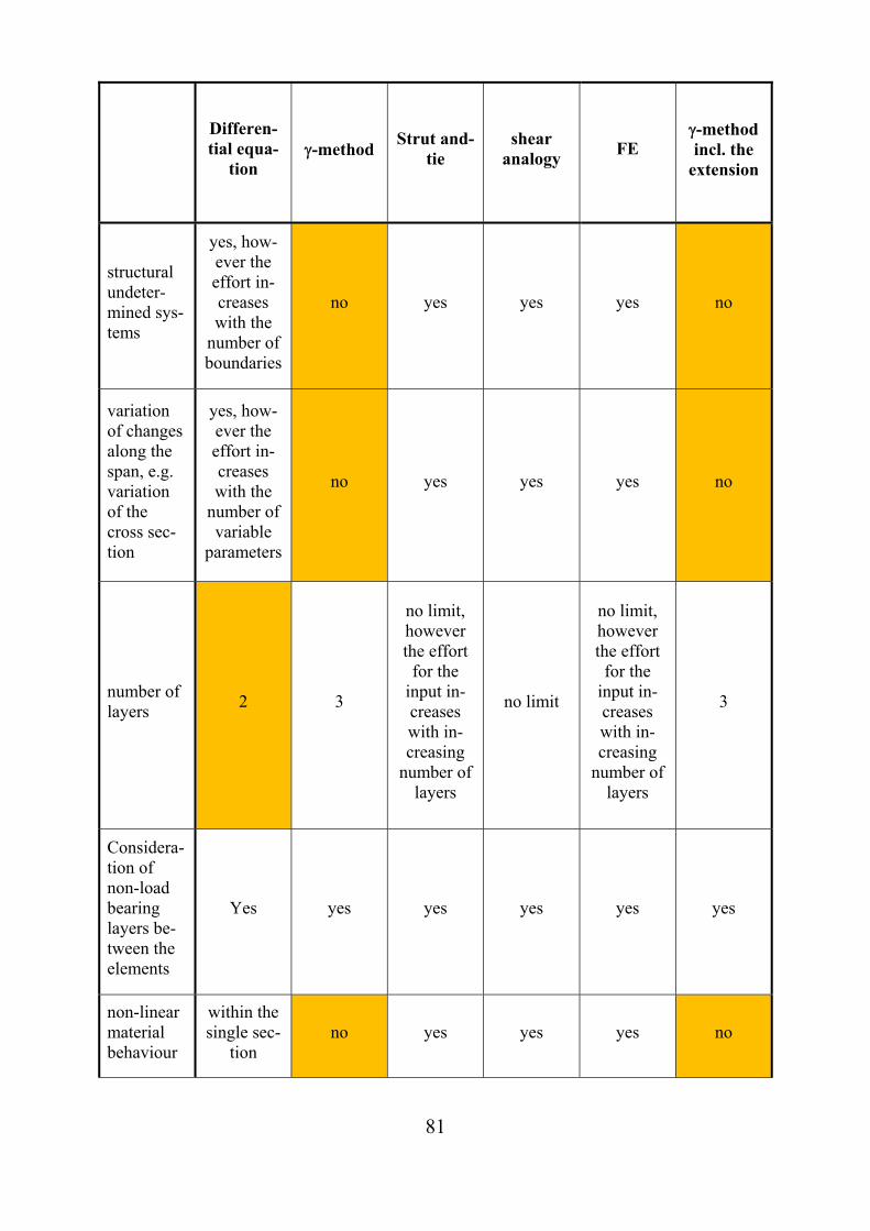
81
Differen-tial equa-
tion -method
Strut and-tie
shear analogy
FE -method incl. the
extension
structural undeter-mined sys-tems
yes, how-ever the effort in-creases with the
number of boundaries
no yes yes yes no
variation of changes along the span, e.g. variation of the cross sec-tion
yes, how-ever the effort in-creases with the
number of variable
parameters
no yes yes yes no
number of layers
2 3
no limit, however the effort
for the input in-creases with in-creasing
number of layers
no limit
no limit, however the effort
for the input in-creases with in-creasing
number of layers
3
Considera-tion of non-load bearing layers be-tween the elements
Yes yes yes yes yes yes
non-linear material behaviour
within the single sec-
tion no yes yes yes no
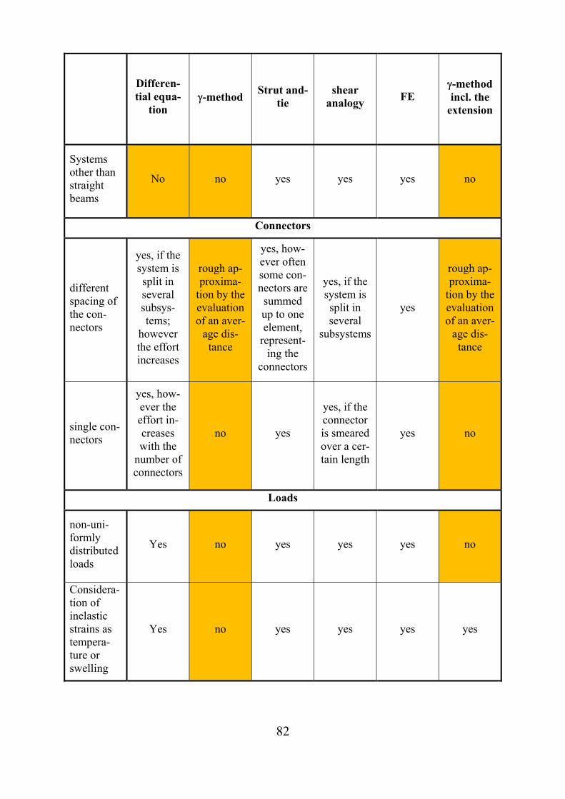
82
Differen-tial equa-
tion -method
Strut and-tie
shear analogy
FE -method incl. the
extension
Systems other than straight beams
No no yes yes yes no
Connectors
different spacing of the con-nectors
yes, if the system is split in several subsys-tems;
however the effort increases
rough ap-proxima-
tion by the evaluation of an aver-
age dis-tance
yes, how-ever often some con-nectors are summed up to one element,
represent-ing the
connectors
yes, if the system is split in several
subsystems
yes
rough ap-proxima-
tion by the evaluation of an aver-
age dis-tance
single con-nectors
yes, how-ever the effort in-creases with the
number of connectors
no yes
yes, if the connector is smeared over a cer-tain length
yes no
Loads
non-uni-formly distributed loads
Yes no yes yes yes no
Considera-tion of inelastic strains as tempera-ture or swelling
Yes no yes yes yes yes
83
As it can be seen in Table 8, the methods have their own range of application:
FE-modelling: Due to the effort and the accuracy of the results the appli-cation of this method will be mainly in the field of development and re-search. However it is not expected, that this method will be part of the dai-ly design.
Differential equation: Due to the high demands concerning the analytical solution, this method will hardly be used in the daily design. Its range of application will be the development of simplified design methods and the discussion of different parameters. So it is expected, that this method will be used in the transition from research to practical design.
Shear-analogy-method: Due to the possibility of modelling several layers with limited efforts, this method will be used in the design if multi layered composite structures with more than 2 layers are evaluated. For example, a multi layered structure is a composite between cross-laminated timber and concrete, where the cross laminated timber has several layers. How-ever it is not expected, that this method is used for the design of “ordi-nary” timber concrete composite structures, since it would require the transfer of the real two-layered system (timber & concrete) into the two systems A and B with modified parameters. Both systems are coupled, targeting at the same deflection. After the evaluation of the internal forces of systems A and B, these forces have to be retransferred. In order to couple both systems, structural analysis software is often used. But when structural analysis software is used for modelling a two layered composite, it is easier to model it directly as strut-and-tie model, since then the real forces in the cross sections are determined. In this case the often already implemented proofs of such software can be used directly (except for the evaluation of the reinforcement; see Sec. 4.3.4).
Strut-and-ties: Since the evaluation of forces by means of strut-and-tie- models is quite familiar for the engineer, it is expected that the design will be often performed with this method. In this method the centroids of the single composite elements are modelled by beams. The connections be-tween the composite elements are also modelled as beams, whereas their properties are adjusted to the stiffness of the connectors. One advantage of this method is that it is not limited to single span system with uniformly distributed loads.
-method: Within this method the effectiveness of the load transfer by normal force is evaluated by means of the so called -value. This -value is considered in the evaluation of the moment of inertia. So from the prac-tical point of view, this method provides an effective bending stiffness, which can be used within a “normal” design. Therefore it is expected, that this method will be used in the design for simple systems as single span girders with uniformly distributed loads. Besides, the evaluation of forces can be performed by hand, so no structural analysis software is necessary.
84
If the system matches the requirements for the application of this method it could be easily used for the evaluation of forces within a spreadsheet program, allowing the optimization of the structure.
As a result of this comparison of the different methods for the evaluation of the forces, it is expected, that the -method and the modelling of composite systems by strut-and-tie models are mainly used in the design process.
However, how to determine the internal forces should not be part of a standard, since the engineer should be able to choose the appropriate method. Neverthe-less the standard should enable the application of the most common methods. Therefore the standard should give rules and recommendations for the applica-tion of these methods. As can be seen in Table 8 rules and recommendations concerning the following influences should be given:
Maximum spacing of the connectors in order to enable the designer to de-sign whether the -method can be used or whether the results will be more accurate, when using the strut-and-ties model
Since the -method is already part of [EN 1995-1-1] Annex B, it should be extended in order to cover the inelastic strains due to temperature or dif-ferent shrinkage/swelling of the composite elements.
4.3.3.2 Maximum spacing In some design methods the connectors are smeared along the beam axis. In this case forces are continuously transferred between the composite elements. There-fore the course of the normal force is affine to the course of the external bending moment. However, the connection itself transfers the forces locally. If discrete connectors are considered, the normal force is constant in between the single connectors, since friction is neglected.
For small spacing, the differences between the constant load transfer through the assumed continuous connection and the discrete load transfer in the connectors is negligible. However if the spacing increases, the difference can become of importance, since the load transfer via normal force can be reduced.
Additionally the location of the connector related to the beam can influence the forces, so smearing the connectors could lead to unacceptable differences be-tween the model and the real forces. In order to limit differences between the “real” internal forces and the modelled internal forces, the distance of the con-nectors has to be determined from which on smearing of the connectors is not acceptable any more.

85
In order to identify this limit, [Niederer, 2008] compared the internal forces evaluated by means of the -method and the strut&tie model for different sys-tems. Within this study the cross sections as well as the properties of the con-nectors have been varied. As it can be seen in Figure 38 and Figure 39 the bend-ing moment according to the -method (assuming smeared connectors) is under-estimated with increasing spacing of the connectors compared to the modelling with a strut & tie model (which is assumed to deliver the correct results).
Figure 38: Influence of the spacing of the connectors on the bending moment, as ratio between the evaluation according to the -method and the modelling as strut&tie model (see [Niederer, 2008])
Figure 39: Influence of the -value on the differences of the bending moment in the timber cross section between the evaluation according to the -method and the strut&tie model (see [Niederer, 2008])
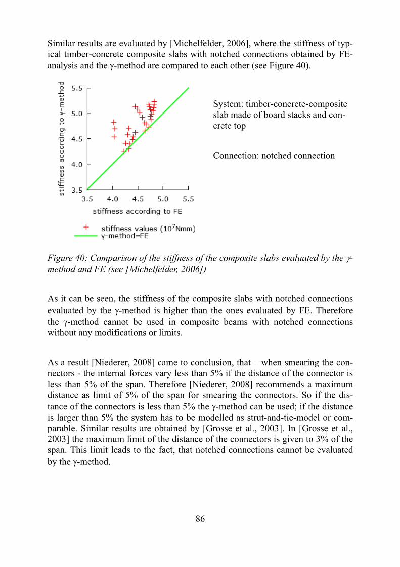
86
Similar results are evaluated by [Michelfelder, 2006], where the stiffness of typ-ical timber-concrete composite slabs with notched connections obtained by FE-analysis and the -method are compared to each other (see Figure 40).
System: timber-concrete-composite slab made of board stacks and con-crete top
Connection: notched connection
Figure 40: Comparison of the stiffness of the composite slabs evaluated by the -method and FE (see [Michelfelder, 2006])
As it can be seen, the stiffness of the composite slabs with notched connections evaluated by the -method is higher than the ones evaluated by FE. Therefore the -method cannot be used in composite beams with notched connections without any modifications or limits.
As a result [Niederer, 2008] came to conclusion, that – when smearing the con-nectors - the internal forces vary less than 5% if the distance of the connector is less than 5% of the span. Therefore [Niederer, 2008] recommends a maximum distance as limit of 5% of the span for smearing the connectors. So if the dis-tance of the connectors is less than 5% the -method can be used; if the distance is larger than 5% the system has to be modelled as strut-and-tie-model or com-parable. Similar results are obtained by [Grosse et al., 2003]. In [Grosse et al., 2003] the maximum limit of the distance of the connectors is given to 3% of the span. This limit leads to the fact, that notched connections cannot be evaluated by the -method.
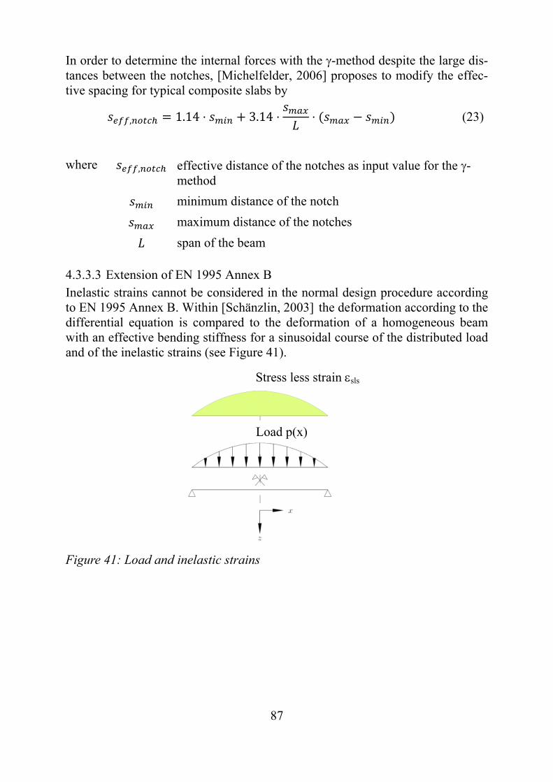
87
In order to determine the internal forces with the -method despite the large dis-tances between the notches, [Michelfelder, 2006] proposes to modify the effec-tive spacing for typical composite slabs by
, 1.14 ⋅ 3.14 ⋅ ⋅ (23)
where , effective distance of the notches as input value for the -method
minimum distance of the notch
maximum distance of the notches
span of the beam
4.3.3.3 Extension of EN 1995 Annex B Inelastic strains cannot be considered in the normal design procedure according to EN 1995 Annex B. Within [Schänzlin, 2003] the deformation according to the differential equation is compared to the deformation of a homogeneous beam with an effective bending stiffness for a sinusoidal course of the distributed load and of the inelastic strains (see Figure 41).
Figure 41: Load and inelastic strains
Load p(x)
Stress less strain sls
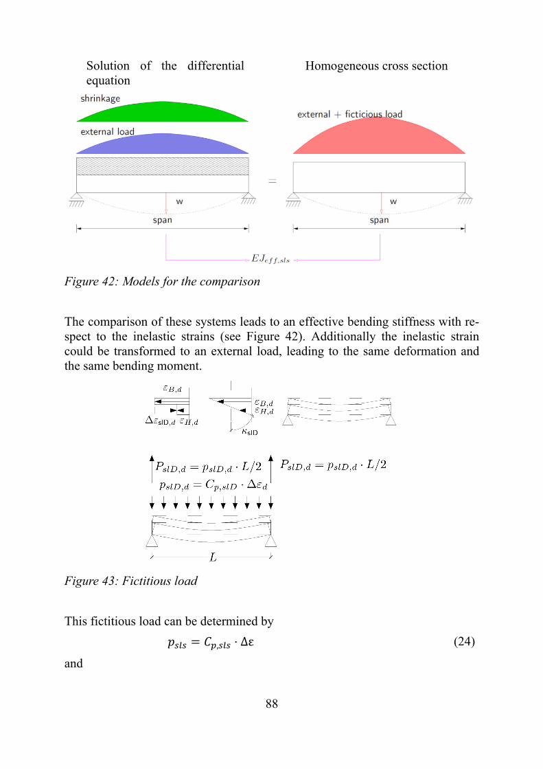
88
Figure 42: Models for the comparison
The comparison of these systems leads to an effective bending stiffness with re-spect to the inelastic strains (see Figure 42). Additionally the inelastic strain could be transformed to an external load, leading to the same deformation and the same bending moment.
Figure 43: Fictitious load
This fictitious load can be determined by
, ⋅ Δε (24)
and
Solution of the differential equation
Homogeneous cross section

89
, ⋅⋅ ⋅ ⋅ ⋅ ⋅⋅ ⋅ ⋅
⋅ (25)
Within this equation the parameter becomes 4,0, if the bending moment is evaluated. The value becomes 4,8 for the evaluation of the deflection. If the ef-fective bending stiffness is evaluated, the parameters of the fictitious load can be
identified. However in this case the -value becomes . For reasons of simpli-
fication it was decided to use solely .
Table 9: Comparison of the effects of shrinkage of concrete on the internal forces and the deflection and the results of modelling this effect solely by a fictitious load
Internal forces Inelastic strain, e.g. shrinkage of concrete
Fictitious load
Deflection Increase Increase
Bending moments in the cross sections
Increase Increase
Normal force in the cross sections
Decrease Increase
Load on the connector Decrease Increase
If this fictitious load is applied on a system, all internal forces and the deflection increase. However, as it can be seen in Table 9, only the bending moment and the deflection increase due to shrinkage. The normal force as well as the load on the connectors behave contrary between the real behaviour and the model.
In order to solve this contradiction between the modelling of the inelastic strains by applying a fictitious load on the system and the real behaviour, the normal force is determined by the equilibrium of forces in midspan. If the normal force is determined by the equilibrium of forces, an overestimation of the bending moment in the single cross section would lead to an underestimation of the nor-mal force.
However using solely the -value = /2, the bending moment is overesti-mated, since in the original derivation the -value is equal 4,0 for the bending moment. In order to correct the overestimation of the bending moment, it is pro-posed not to consider the bending moment under the full fictitious load but only
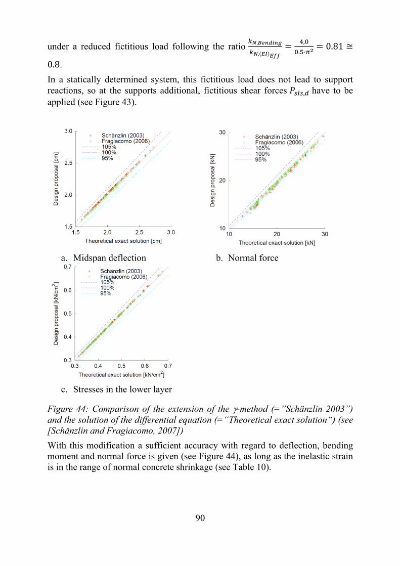
90
under a reduced fictitious load following the ratio ,
,
,
. ⋅0.81 ≅
0.8.
In a statically determined system, this fictitious load does not lead to support reactions, so at the supports additional, fictitious shear forces , have to be applied (see Figure 43).
a. Midspan deflection b. Normal force
c. Stresses in the lower layer
Figure 44: Comparison of the extension of the -method (=”Schänzlin 2003”) and the solution of the differential equation (=“Theoretical exact solution“) (see [Schänzlin and Fragiacomo, 2007])
With this modification a sufficient accuracy with regard to deflection, bending moment and normal force is given (see Figure 44), as long as the inelastic strain is in the range of normal concrete shrinkage (see Table 10).
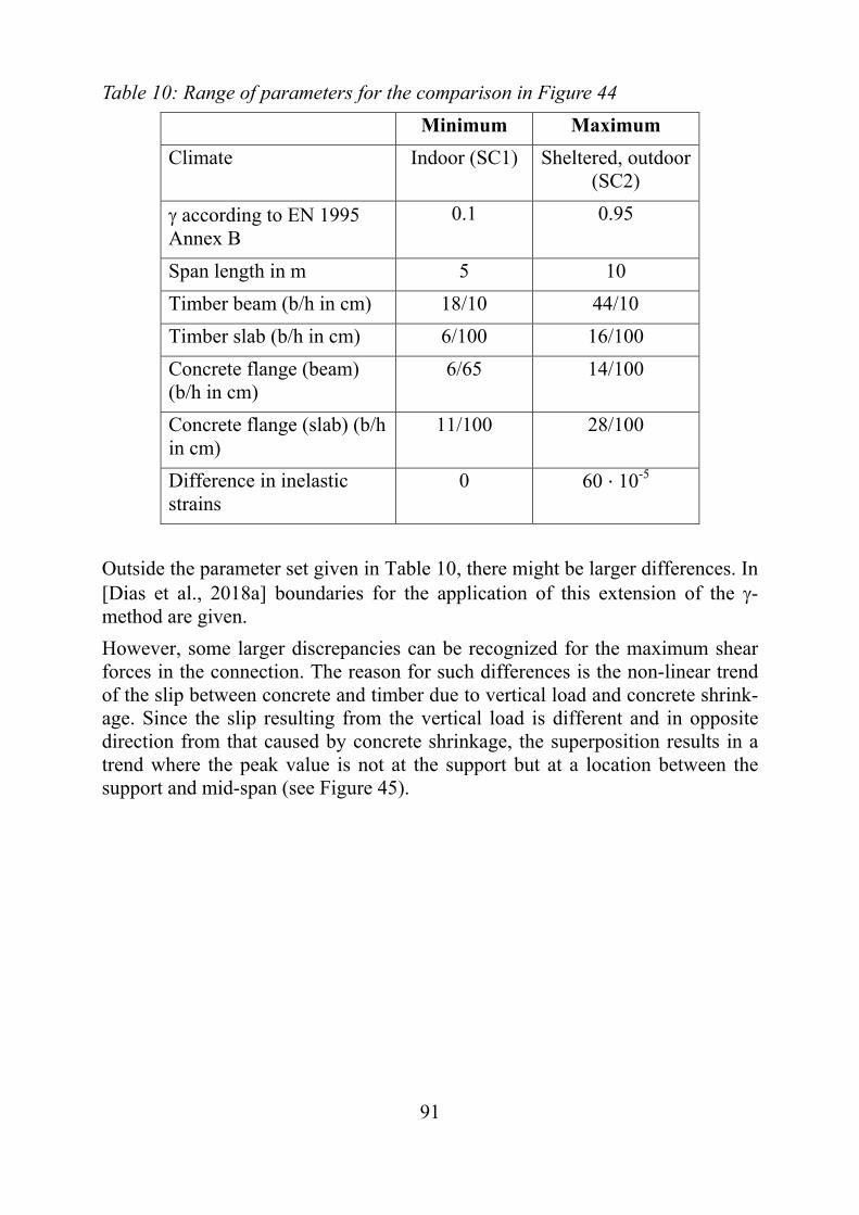
91
Table 10: Range of parameters for the comparison in Figure 44
Minimum Maximum
Climate Indoor (SC1) Sheltered, outdoor (SC2)
according to EN 1995 Annex B
0.1 0.95
Span length in m 5 10
Timber beam (b/h in cm) 18/10 44/10
Timber slab (b/h in cm) 6/100 16/100
Concrete flange (beam) (b/h in cm)
6/65 14/100
Concrete flange (slab) (b/h in cm)
11/100 28/100
Difference in inelastic strains
0 60 ⋅ 10-5
Outside the parameter set given in Table 10, there might be larger differences. In [Dias et al., 2018a] boundaries for the application of this extension of the -method are given.
However, some larger discrepancies can be recognized for the maximum shear forces in the connection. The reason for such differences is the non-linear trend of the slip between concrete and timber due to vertical load and concrete shrink-age. Since the slip resulting from the vertical load is different and in opposite direction from that caused by concrete shrinkage, the superposition results in a trend where the peak value is not at the support but at a location between the support and mid-span (see Figure 45).
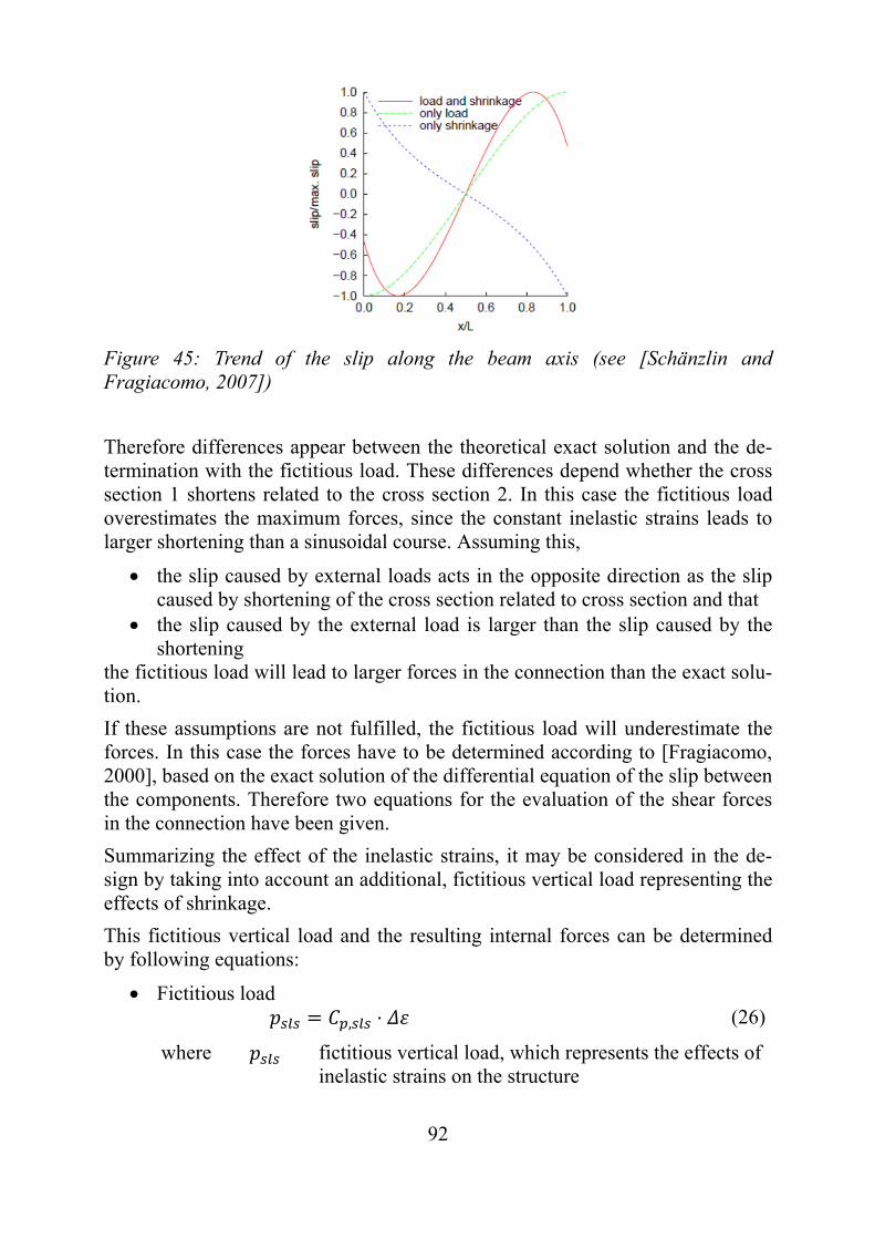
92
Figure 45: Trend of the slip along the beam axis (see [Schänzlin and Fragiacomo, 2007])
Therefore differences appear between the theoretical exact solution and the de-termination with the fictitious load. These differences depend whether the cross section 1 shortens related to the cross section 2. In this case the fictitious load overestimates the maximum forces, since the constant inelastic strains leads to larger shortening than a sinusoidal course. Assuming this,
the slip caused by external loads acts in the opposite direction as the slip caused by shortening of the cross section related to cross section and that
the slip caused by the external load is larger than the slip caused by the shortening
the fictitious load will lead to larger forces in the connection than the exact solu-tion.
If these assumptions are not fulfilled, the fictitious load will underestimate the forces. In this case the forces have to be determined according to [Fragiacomo, 2000], based on the exact solution of the differential equation of the slip between the components. Therefore two equations for the evaluation of the shear forces in the connection have been given.
Summarizing the effect of the inelastic strains, it may be considered in the de-sign by taking into account an additional, fictitious vertical load representing the effects of shrinkage.
This fictitious vertical load and the resulting internal forces can be determined by following equations:
Fictitious load , ⋅ (26)
where fictitious vertical load, which represents the effects of inelastic strains on the structure
93
, coefficient
⋅⋅ ⋅ ⋅ ⋅ ⋅
⋅ ⋅ ⋅⋅
difference in the inelastic strain between cross section 2 and the cross section 1
/2
Effective bending stiffness , , ⋅ (27)
where , effective bending stiffness with respect to the inelas-tic strains
effective bending stiffness according to EC5 Annex B, Eq. (B.1)
, coefficient, which considers the interaction between vertical load qd and inelastic strains in terms of slip in the joint
⋅ ⋅
⋅ ⋅ ⋅ ⋅
coefficient calculated according to EC5 Annex B, Eq. (B.5)
Bending moment in the cross section: The bending moment within the single cross section can be evaluated by
⋅
,⋅ 0.8 ⋅
(28)
where , effective bending stiffness according to EC5 Annex B which accounts for the interaction between vertical load and inelastic strains (see Eq. (18))
bending moment of the component i
0.8 ⋅ resulting bending moment due to vertical load and part (80%) of the fictitious load equivalent to inelastic strains
Normal forces: The normal forces are determined using the equilibrium equation:
94
∑ (29)
where resulting bending moment due to vertical load on-ly
distance between the centroids of the concrete slab and timber beam
Shear forces: The shear force in the connector can be determined accord-ing to EN 1995 Annex B Eq. (B.10) (see [EN 1995-1-1]) if the shear force is evaluated by following equation assuming that the cross section 1 (=cross section in compression) shortens related to cross section 2:
, ⋅ ⋅ ⋅⋅ ⋅
⋅ ⋅ ⋅ ⋅ ⋅ ⋅⋅ Δ
(30)
where resulting shear force due to vertical load only, cal-culated using the formulas (Eq. B.10) suggested by the Annex B of the EC5.
In the other case – when cross section 2 (=cross section in tension) short-ens related to cross section 1, the shear force in the connector can be de-termined by following equation:
⋅ ⋅ , ⋅⋅ ⋅
⋅ ⋅⋅ ⋅ ⋅ ⋅
⋅ ,Δ2
(31)
4.3.4 Cracking of concrete and moment-rotation relation
4.3.4.1 Effect on the stiffness The design of concrete structures is given in [EN 1992-1-1]. Within this stand-ard, the stress strain relation for concrete is given, which is characterized by
No consideration of the tension force except for the determination of the capacity for the shear forces
Stress-strain-relation for the evaluation of the internal forces according to the following equation (see Figure 46)
⋅⋅
1 2 ⋅
(32)
where coefficient
1,05 ⋅ ⋅ ,
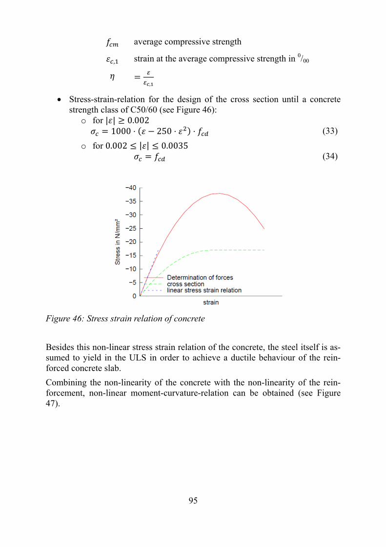
95
average compressive strength
, strain at the average compressive strength in 0/00
,
Stress-strain-relation for the design of the cross section until a concrete strength class of C50/60 (see Figure 46):
o for | | 0.002 1000 ⋅ 250 ⋅ ⋅ (33)
o for 0.002 | | 0.0035 (34)
Figure 46: Stress strain relation of concrete
Besides this non-linear stress strain relation of the concrete, the steel itself is as-sumed to yield in the ULS in order to achieve a ductile behaviour of the rein-forced concrete slab.
Combining the non-linearity of the concrete with the non-linearity of the rein-forcement, non-linear moment-curvature-relation can be obtained (see Figure 47).
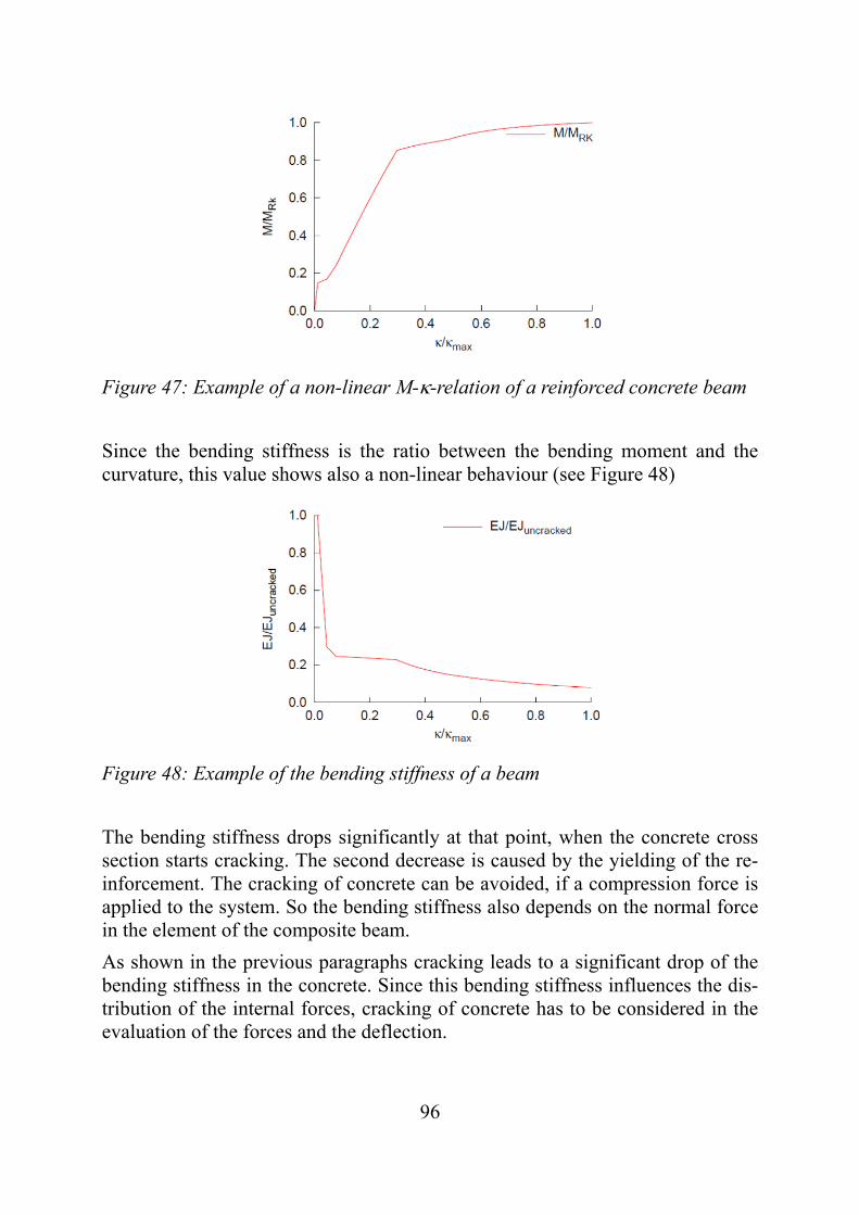
96
Figure 47: Example of a non-linear M--relation of a reinforced concrete beam
Since the bending stiffness is the ratio between the bending moment and the curvature, this value shows also a non-linear behaviour (see Figure 48)
Figure 48: Example of the bending stiffness of a beam
The bending stiffness drops significantly at that point, when the concrete cross section starts cracking. The second decrease is caused by the yielding of the re-inforcement. The cracking of concrete can be avoided, if a compression force is applied to the system. So the bending stiffness also depends on the normal force in the element of the composite beam.
As shown in the previous paragraphs cracking leads to a significant drop of the bending stiffness in the concrete. Since this bending stiffness influences the dis-tribution of the internal forces, cracking of concrete has to be considered in the evaluation of the forces and the deflection.
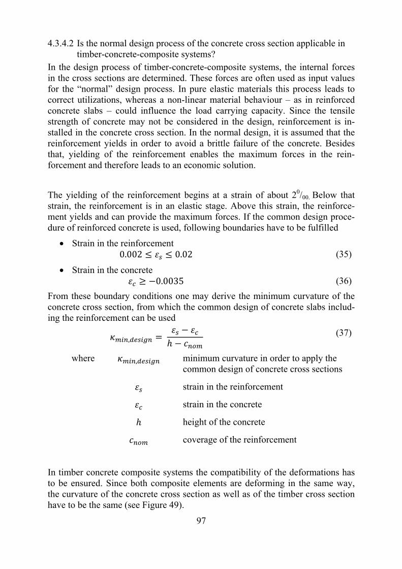
97
4.3.4.2 Is the normal design process of the concrete cross section applicable in timber-concrete-composite systems?
In the design process of timber-concrete-composite systems, the internal forces in the cross sections are determined. These forces are often used as input values for the “normal” design process. In pure elastic materials this process leads to correct utilizations, whereas a non-linear material behaviour – as in reinforced concrete slabs – could influence the load carrying capacity. Since the tensile strength of concrete may not be considered in the design, reinforcement is in-stalled in the concrete cross section. In the normal design, it is assumed that the reinforcement yields in order to avoid a brittle failure of the concrete. Besides that, yielding of the reinforcement enables the maximum forces in the rein-forcement and therefore leads to an economic solution.
The yielding of the reinforcement begins at a strain of about 20/00. Below that strain, the reinforcement is in an elastic stage. Above this strain, the reinforce-ment yields and can provide the maximum forces. If the common design proce-dure of reinforced concrete is used, following boundaries have to be fulfilled
Strain in the reinforcement 0.002 0.02 (35)
Strain in the concrete 0.0035 (36)
From these boundary conditions one may derive the minimum curvature of the concrete cross section, from which the common design of concrete slabs includ-ing the reinforcement can be used
, (37)
where , minimum curvature in order to apply the common design of concrete cross sections
strain in the reinforcement
strain in the concrete
height of the concrete
coverage of the reinforcement
In timber concrete composite systems the compatibility of the deformations has to be ensured. Since both composite elements are deforming in the same way, the curvature of the concrete cross section as well as of the timber cross section have to be the same (see Figure 49).
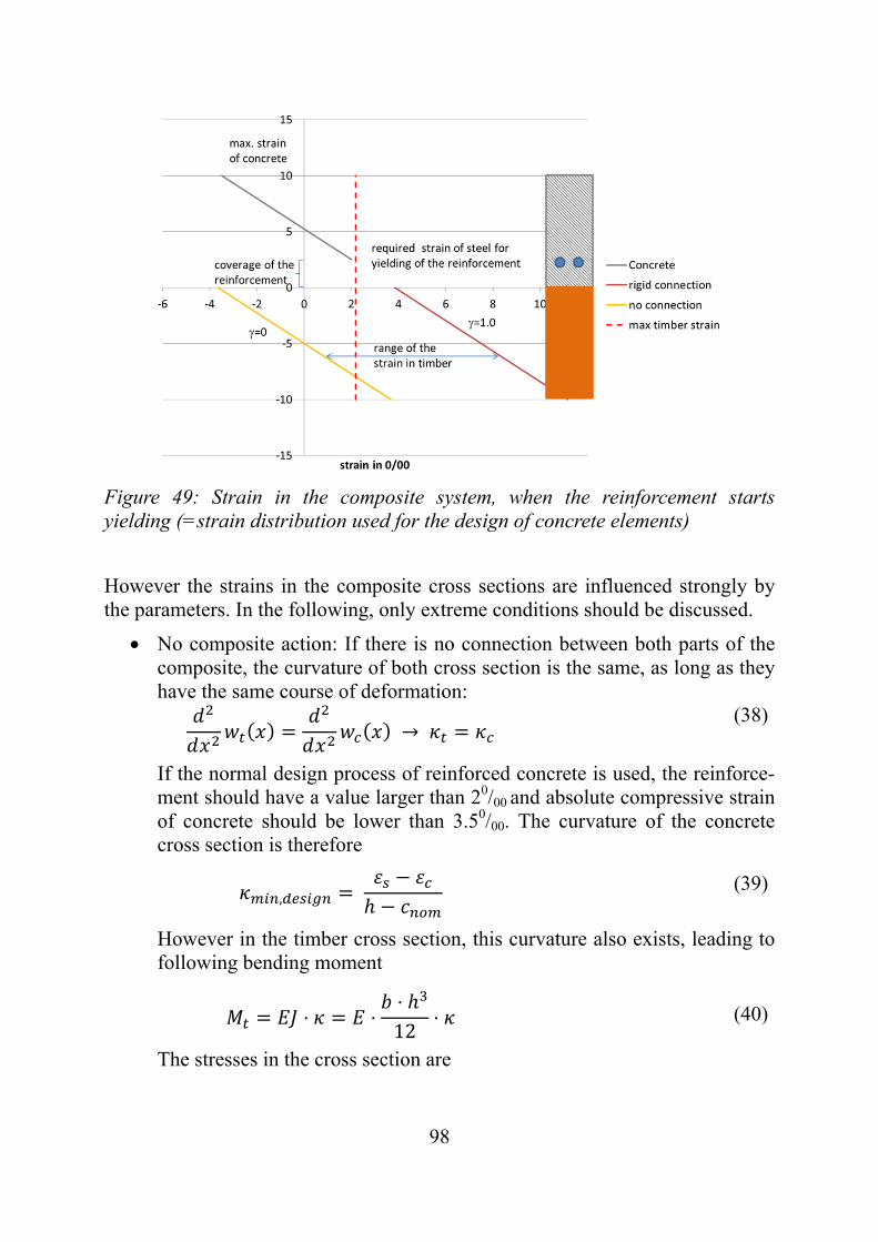
98
Figure 49: Strain in the composite system, when the reinforcement starts yielding (=strain distribution used for the design of concrete elements)
However the strains in the composite cross sections are influenced strongly by the parameters. In the following, only extreme conditions should be discussed.
No composite action: If there is no connection between both parts of the composite, the curvature of both cross section is the same, as long as they have the same course of deformation:
→ (38)
If the normal design process of reinforced concrete is used, the reinforce-ment should have a value larger than 20/00 and absolute compressive strain of concrete should be lower than 3.50/00. The curvature of the concrete cross section is therefore
, (39)
However in the timber cross section, this curvature also exists, leading to following bending moment
⋅ ⋅⋅12
⋅ (40)
The stresses in the cross section are
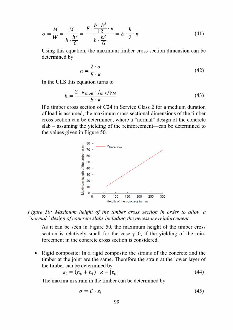
99
⋅ 6
⋅
⋅12 ⋅
⋅ 6
⋅2⋅ (41)
Using this equation, the maximum timber cross section dimension can be determined by
2 ⋅⋅
(42)
In the ULS this equation turns to
2 ⋅ ⋅ , /⋅
(43)
If a timber cross section of C24 in Service Class 2 for a medium duration of load is assumed, the maximum cross sectional dimensions of the timber cross section can be determined, where a “normal” design of the concrete slab – assuming the yielding of the reinforcement—can be determined to the values given in Figure 50.
Figure 50: Maximum height of the timber cross section in order to allow a “normal” design of concrete slabs including the necessary reinforcement
As it can be seen in Figure 50, the maximum height of the timber cross section is relatively small for the case =0, if the yielding of the rein-forcement in the concrete cross section is considered.
Rigid composite: In a rigid composite the strains of the concrete and the timber at the joint are the same. Therefore the strain at the lower layer of the timber can be determined by
⋅ | | (44)
The maximum strain in the timber can be determined by
⋅ (45)
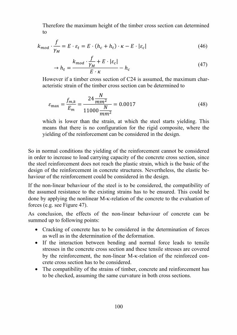
100
Therefore the maximum height of the timber cross section can determined to
⋅ ⋅ ⋅ ⋅ ⋅ | | (46)
→⋅ ⋅ | |
⋅
(47)
However if a timber cross section of C24 is assumed, the maximum char-acteristic strain of the timber cross section can be determined to
,24
110000.0017 (48)
which is lower than the strain, at which the steel starts yielding. This means that there is no configuration for the rigid composite, where the yielding of the reinforcement can be considered in the design.
So in normal conditions the yielding of the reinforcement cannot be considered in order to increase to load carrying capacity of the concrete cross section, since the steel reinforcement does not reach the plastic strain, which is the basic of the design of the reinforcement in concrete structures. Nevertheless, the elastic be-haviour of the reinforcement could be considered in the design.
If the non-linear behaviour of the steel is to be considered, the compatibility of the assumed resistance to the existing strains has to be ensured. This could be done by applying the nonlinear M--relation of the concrete to the evaluation of forces (e.g. see Figure 47).
As conclusion, the effects of the non-linear behaviour of concrete can be summed up to following points:
Cracking of concrete has to be considered in the determination of forces as well as in the determination of the deformation.
If the interaction between bending and normal force leads to tensile stresses in the concrete cross section and these tensile stresses are covered by the reinforcement, the non-linear M--relation of the reinforced con-crete cross section has to be considered.
The compatibility of the strains of timber, concrete and reinforcement has to be checked, assuming the same curvature in both cross sections.
101
4.3.5 Stress-strain relation for the evaluation of internal forces
In [EN 1992-1-1] the stress-strain-relation for the determination of the internal forces is given by
⋅⋅
1 2 ⋅ (49)
where coefficient
1,05 ⋅ ⋅ ,
average compressive strength
, strain at the average compressive strength in 0/00
,
However for practical use, this non-linear stress-strain-relation can hardly be applied, since it would lead to different MoEs along the beam axis. For simplifi-cation it is recommended to use the linear stress strain relation up to the design value of the ultimate strength of concrete.
In order to determine the MoE, the inclination of the stress-strain-relation is de-termined by
(50)
and therefore
⋅⋅
1 2 ⋅ (51)
If the MoE is determined in the range between 0 and , the value of the MoE varies between
, 1.05 ⋅ , (52)
This assumes that the maximum stresses are evaluated in the design
, , (53)
However the stresses should be smaller than the design value of the compressive strength, leading to
102
, ⋅ , 0.85 ⋅ ,
1.5 (54)
As can be seen in Figure 51 the MoE in design situations varies between the fol-lowing boundaries
~0.9 ⋅ , 1.05 ⋅ , (55)
Figure 51: MoE of concrete in dependence of the strain
Since the differences of the MoE in the range between 0 and the strain caused by the maximum design stresses are small, the influence of the stresses on the MoE can be neglected. Therefore a linear stress-strain-relation and a con-stant MoE can be used. [EN 1992-1-1] 5.4 also proposes to use the average val-ue of the MoE for the determination of the internal forces.
4.3.6 Effective width
The external bending moment is divided into the bending moments and the nor-mal forces in the cross section.
⋅ (56)
where external bending force
bending force in cross section 1
bending moment in cross section 2
normal force in both cross sections
distance between the centroids of both cross sections (=inner lever arm)
Due to the linear load transfer parallel to the span, the concrete cross section is distributing its load by shear and bending (see Figure 52).
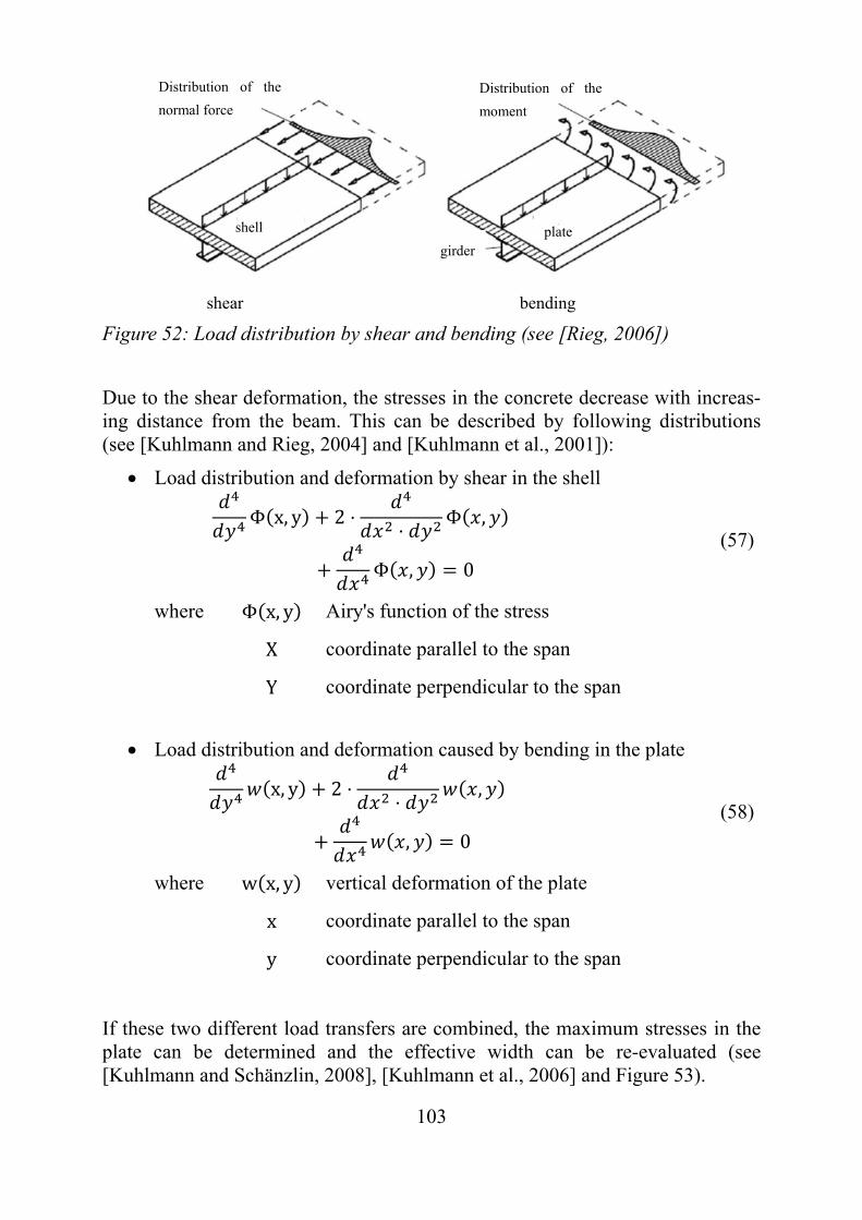
103
shear bending
Figure 52: Load distribution by shear and bending (see [Rieg, 2006])
Due to the shear deformation, the stresses in the concrete decrease with increas-ing distance from the beam. This can be described by following distributions (see [Kuhlmann and Rieg, 2004] and [Kuhlmann et al., 2001]):
Load distribution and deformation by shear in the shell
Φ x, y 2 ⋅⋅
Φ ,
Φ , 0
(57)
where Φ x, y Airy's function of the stress
X coordinate parallel to the span
Y coordinate perpendicular to the span
Load distribution and deformation caused by bending in the plate
x, y 2 ⋅⋅
,
, 0
(58)
where w x, y vertical deformation of the plate
x coordinate parallel to the span
y coordinate perpendicular to the span
If these two different load transfers are combined, the maximum stresses in the plate can be determined and the effective width can be re-evaluated (see [Kuhlmann and Schänzlin, 2008], [Kuhlmann et al., 2006] and Figure 53).
Distribution of the
moment
Distribution of the
normal force
plate shell
girder
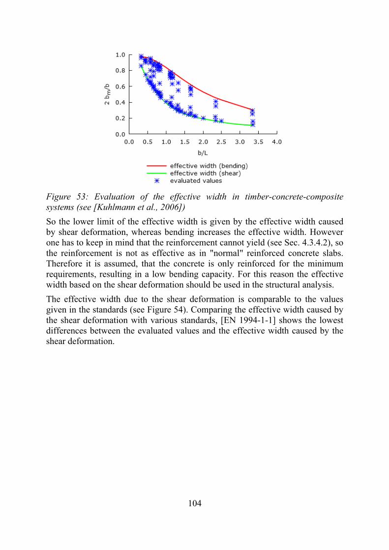
104
Figure 53: Evaluation of the effective width in timber-concrete-composite systems (see [Kuhlmann et al., 2006])
So the lower limit of the effective width is given by the effective width caused by shear deformation, whereas bending increases the effective width. However one has to keep in mind that the reinforcement cannot yield (see Sec. 4.3.4.2), so the reinforcement is not as effective as in "normal" reinforced concrete slabs. Therefore it is assumed, that the concrete is only reinforced for the minimum requirements, resulting in a low bending capacity. For this reason the effective width based on the shear deformation should be used in the structural analysis.
The effective width due to the shear deformation is comparable to the values given in the standards (see Figure 54). Comparing the effective width caused by the shear deformation with various standards, [EN 1994-1-1] shows the lowest differences between the evaluated values and the effective width caused by the shear deformation.
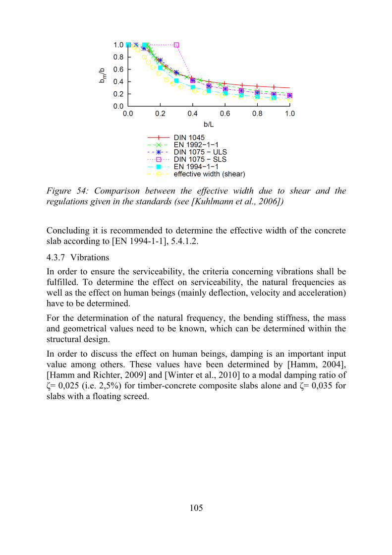
105
Figure 54: Comparison between the effective width due to shear and the regulations given in the standards (see [Kuhlmann et al., 2006])
Concluding it is recommended to determine the effective width of the concrete slab according to [EN 1994-1-1], 5.4.1.2.
4.3.7 Vibrations
In order to ensure the serviceability, the criteria concerning vibrations shall be fulfilled. To determine the effect on serviceability, the natural frequencies as well as the effect on human beings (mainly deflection, velocity and acceleration) have to be determined.
For the determination of the natural frequency, the bending stiffness, the mass and geometrical values need to be known, which can be determined within the structural design.
In order to discuss the effect on human beings, damping is an important input value among others. These values have been determined by [Hamm, 2004], [Hamm and Richter, 2009] and [Winter et al., 2010] to a modal damping ratio of ζ= 0,025 (i.e. 2,5%) for timber-concrete composite slabs alone and ζ= 0,035 for slabs with a floating screed.
106
4.4 Long term behaviour / consideration of creep and shrinkage
4.4.1 Creep and shrinkage
The composite system must fulfil the requirements over the whole lifetime of the building. Therefore it is not sufficient to consider only the short term behaviour directly after installation. Over time, some effects may occur, which influences the internal forces as well as the deformation. The most important effects are (see among others [Kenel and Meierhofer, 1998], [Schmidt et al., 2003], [Schmidt et al., 2004] and [Jorge et al., 2010])
Creep of the material: If a system is loaded, it deforms. If the system is loaded over a certain time, the deformation increases over time. This addi-tional deformation is called creep deformation.
Shrinkage and/or swelling of the material: If materials are hardening by means of a chemical reaction or interact with the surrounding by absorb-ing or emitting moisture, often the volume of the material changes. In the first case, the reaction product embeds the elements in a new order, so the volume is reduced and the cross section shrinks. In the second case water is embedded in the structure, so the volume increases. If moisture is emit-ted, the volume decreases and the cross section shrinks. Since this strain is independent on stresses, it is often called inelastic strains. The effect of shrinkage and swelling on the stresses and the deformation is comparable to the effect of changing temperature in a composite system of compo-nents with different thermal expansion coefficients.
The effects of the creep deformations in a composite system are
Deformation: Due to the creep deformation of at least one of the compo-nents (here timber, concrete and connection), the deformation increases. Timber-concrete composite systems are often applied for spans larger than 5m. In this range of application often the limitation of the deformation is the decisive verification.
Internal stresses and forces: The creep strain can be interpreted as a reduc-tion of the stiffness. Since the stiffness is one essential influence of the distribution of the loads in statically undetermined systems, creep strains could change the distribution of loads within a composite system. This re-distribution increases the larger the difference between the creep coeffi-cients of the single components is. If one component is creeping stronger than the other, the stronger creeping component will reduce its load. Due to the equilibrium of forces the less creeping component will receive higher loads. Additionally the normal force will be also affected by the creep strain. Fi-nally the bending moment of the less creeping component will be in-

107
creased whereas the normal force will decrease. In the end, the stresses in the less creeping component will increase.
The effects of shrinkage are (see Figure 35):
Deformation: If the upper component shortens and this shortening is blocked by the connectors, an internal bending moment arises, which lead to an increase of the deflection. In timber concrete composite structures this increase of the deflection due to shrinkage of the concrete could reach values comparable to the defor-mation caused by the dead load. Therefore this part of the deflection can-not be neglected.
Internal forces: if the upper component (which is compressed) shrinks, the normal force in the components will decrease, whereas the bending mo-ment increases. Since a larger part is transferred by bending, the system becomes softer and the stresses in the lower layer increase. This increase and the eigenstresses should be covered by the design process, since tim-ber is rather brittle. So the eigenstresses could not be reduced by yielding as it is in steel-concrete or pure concrete structures.
For these reasons it is not only sufficient to consider the initial but also the long term behaviour of the materials.
4.4.2 Development of the creep strain over time
In the design all critical points in time have to be considered. Normally "only" the points in time 0 and ∞ are considered. In order to consider the creep strain, an effective Modulus of Elasticity is used
1 ⋅ (59)
This effective MoE is an input value for the determination of the internal forces. According to [EN 1995-1-1] Annex B the effective bending stiffness can be de-termined by
⋅ ⋅⋅ ⋅
(60)
where
ratio of the Moduli of Elasticity of both components at a certain point in time .
With this effective bending stiffness, the internal forces of the timber cross sec-tion can be determined by the following equations
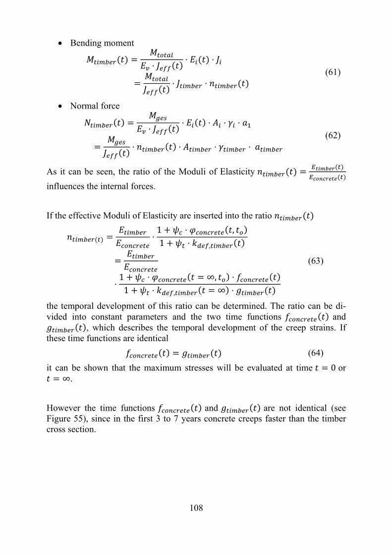
108
Bending moment
⋅⋅ ⋅
⋅ ⋅ (61)
Normal force
⋅⋅ ⋅ ⋅ ⋅
⋅ ⋅ ⋅ ⋅ (62)
As it can be seen, the ratio of the Moduli of Elasticity
influences the internal forces.
If the effective Moduli of Elasticity are inserted into the ratio
⋅1 ⋅ ,1 ⋅ ,
⋅1 ⋅ ∞, ⋅1 ⋅ , ∞ ⋅
(63)
the temporal development of this ratio can be determined. The ratio can be di-vided into constant parameters and the two time functions and
, which describes the temporal development of the creep strains. If these time functions are identical
(64)
it can be shown that the maximum stresses will be evaluated at time 0 or ∞.
However the time functions and are not identical (see Figure 55), since in the first 3 to 7 years concrete creeps faster than the timber cross section.
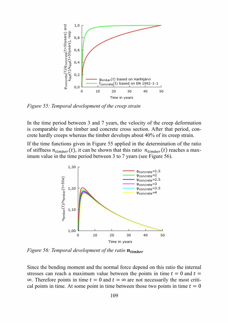
109
Figure 55: Temporal development of the creep strain
In the time period between 3 and 7 years, the velocity of the creep deformation is comparable in the timber and concrete cross section. After that period, con-crete hardly creeps whereas the timber develops about 40% of its creep strain.
If the time functions given in Figure 55 applied in the determination of the ratio of stiffness , it can be shown that this ratio reaches a max-imum value in the time period between 3 to 7 years (see Figure 56).
Figure 56: Temporal development of the ratio
Since the bending moment and the normal force depend on this ratio the internal stresses can reach a maximum value between the points in time 0 and ∞. Therefore points in time 0 and ∞ are not necessarily the most criti-cal points in time. At some point in time between those two points in time 0
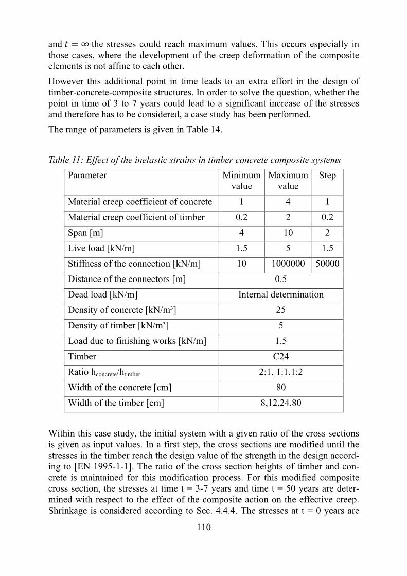
110
and ∞ the stresses could reach maximum values. This occurs especially in those cases, where the development of the creep deformation of the composite elements is not affine to each other.
However this additional point in time leads to an extra effort in the design of timber-concrete-composite structures. In order to solve the question, whether the point in time of 3 to 7 years could lead to a significant increase of the stresses and therefore has to be considered, a case study has been performed.
The range of parameters is given in Table 14.
Table 11: Effect of the inelastic strains in timber concrete composite systems
Parameter Minimum value
Maximum value
Step
Material creep coefficient of concrete 1 4 1
Material creep coefficient of timber 0.2 2 0.2
Span [m] 4 10 2
Live load [kN/m] 1.5 5 1.5
Stiffness of the connection [kN/m] 10 1000000 50000
Distance of the connectors [m] 0.5
Dead load [kN/m] Internal determination
Density of concrete [kN/m³] 25
Density of timber [kN/m³] 5
Load due to finishing works [kN/m] 1.5
Timber C24
Ratio hconcrete/htimber 2:1, 1:1,1:2
Width of the concrete [cm] 80
Width of the timber [cm] 8,12,24,80
Within this case study, the initial system with a given ratio of the cross sections is given as input values. In a first step, the cross sections are modified until the stresses in the timber reach the design value of the strength in the design accord-ing to [EN 1995-1-1]. The ratio of the cross section heights of timber and con-crete is maintained for this modification process. For this modified composite cross section, the stresses at time t = 3-7 years and time t = 50 years are deter-mined with respect to the effect of the composite action on the effective creep. Shrinkage is considered according to Sec. 4.4.4. The stresses at t = 0 years are
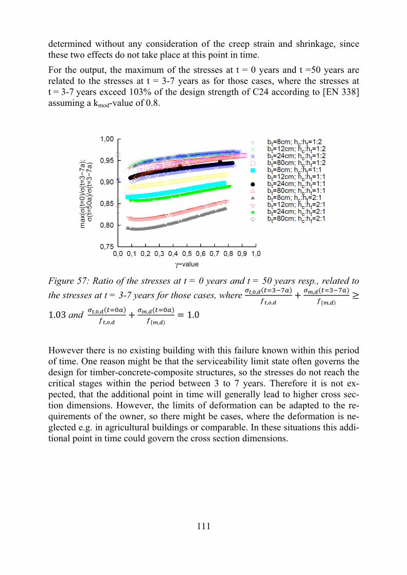
111
determined without any consideration of the creep strain and shrinkage, since these two effects do not take place at this point in time.
For the output, the maximum of the stresses at t = 0 years and t =50 years are related to the stresses at t = 3-7 years as for those cases, where the stresses at t = 3-7 years exceed 103% of the design strength of C24 according to [EN 338] assuming a kmod-value of 0.8.
Figure 57: Ratio of the stresses at t = 0 years and t = 50 years resp., related to
the stresses at t = 3-7 years for those cases, where , ,
, ,
,
,
1.03 and , ,
, ,
,
,1.0
However there is no existing building with this failure known within this period of time. One reason might be that the serviceability limit state often governs the design for timber-concrete-composite structures, so the stresses do not reach the critical stages within the period between 3 to 7 years. Therefore it is not ex-pected, that the additional point in time will generally lead to higher cross sec-tion dimensions. However, the limits of deformation can be adapted to the re-quirements of the owner, so there might be cases, where the deformation is ne-glected e.g. in agricultural buildings or comparable. In these situations this addi-tional point in time could govern the cross section dimensions.

112
4.4.3 Composite creep coefficients
The time dependent strain is given by
(65)
So the changes within are described by
(66)
The changes in the creep strain can be expressed according to [Dischinger, 1939]
⋅ (67)
leading to
⋅ (68)
Assuming a constant MoE over time, this differential equation can be modified by
→1⋅ (69)
leading to
1⋅ ⋅ (70)
This equation can be solved for different boundary conditions. However there are two extremal situations:
Statically determined system: In this system, inelastic strains do not lead to any stresses. Therefore the stress is constant over time leading to
0 (71)
and
⋅ (72)
The solution is given by
⋅ (73)
Since at t = 0 years no creep strain has occurred the constant C can be de-termined to
113
(74)
leading to
⋅ 1 (75)
Introducing an effective MoE in order to determine the total strain by
⋅ 1 (76)
this effective MoE can be determined to
1
(77)
Clamped system: In a clamped system the strain is constant over time. Therefore the basic differential equation turns into
01⋅ ⋅ (78)
and simplified
0 (79)
For the boundary conditions o 0 0 o 0
the solution of this differential equation is
⋅ exp (80)
In this system the strain is constant over time, so the basic equation is val-id
(81)
The creep strain is expressed as
⋆ ⋅ (82)
which leads to the effective MoE of
1 ⋆ (83)
However the total strain is expressed by
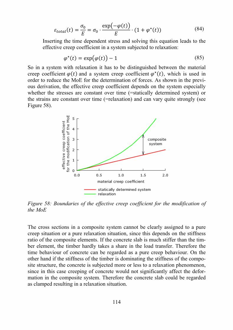
114
⋅exp
⋅ 1 ⋆ (84)
Inserting the time dependent stress and solving this equation leads to the effective creep coefficient in a system subjected to relaxation:
⋆ exp 1 (85)
So in a system with relaxation it has to be distinguished between the material creep coefficient and a system creep coefficient ⋆ , which is used in order to reduce the MoE for the determination of forces. As shown in the previ-ous derivation, the effective creep coefficient depends on the system especially whether the stresses are constant over time (=statically determined system) or the strains are constant over time (=relaxation) and can vary quite strongly (see Figure 58).
Figure 58: Boundaries of the effective creep coefficient for the modification of the MoE
The cross sections in a composite system cannot be clearly assigned to a pure creep situation or a pure relaxation situation, since this depends on the stiffness ratio of the composite elements. If the concrete slab is much stiffer than the tim-ber element, the timber hardly takes a share in the load transfer. Therefore the time behaviour of concrete can be regarded as a pure creep behaviour. On the other hand if the stiffness of the timber is dominating the stiffness of the compo-site structure, the concrete is subjected more or less to a relaxation phenomenon, since in this case creeping of concrete would not significantly affect the defor-mation in the composite system. Therefore the concrete slab could be regarded as clamped resulting in a relaxation situation.
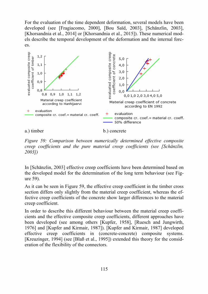
115
For the evaluation of the time dependent deformation, several models have been developed (see [Fragiacomo, 2000], [Bou Saïd, 2003], [Schänzlin, 2003], [Khorsandnia et al., 2014] or [Khorsandnia et al., 2015]). These numerical mod-els describe the temporal development of the deformation and the internal forc-es.
a.) timber b.) concrete
Figure 59: Comparison between numerically determined effective composite creep coefficients and the pure material creep coefficients (see [Schänzlin, 2003])
In [Schänzlin, 2003] effective creep coefficients have been determined based on the developed model for the determination of the long term behaviour (see Fig-ure 59).
As it can be seen in Figure 59, the effective creep coefficient in the timber cross section differs only slightly from the material creep coefficient, whereas the ef-fective creep coefficients of the concrete show larger differences to the material creep coefficient.
In order to describe this different behaviour between the material creep coeffi-cients and the effective composite creep coefficients, different approaches have been developed (see among others [Kupfer, 1958], [Ruesch and Jungwirth, 1976] and [Kupfer and Kirmair, 1987]). [Kupfer and Kirmair, 1987] developed effective creep coefficients in (concrete-concrete) composite systems. [Kreuzinger, 1994] (see [Blaß et al., 1995]) extended this theory for the consid-eration of the flexibility of the connectors.
116
According to this theory the effective creep coefficient (=”composite creep coef-ficients”) of the cross section i in a composite system made of two different ma-terials can be determined by
, , ⋅1 ,
, exp ⋅
1 (86)
where , effective creep coefficient of the cross section i for the modification of the MoE in the structural analy-sis
, material creep coefficient of the cross section i
, material creep coefficient of the cross section j
composite creep coefficient
The composite creep coefficient is defined as
⋅ , ⋅ ,
where composite creep coefficient
, material creep coefficient of the cross section i
, material creep coefficient of the cross section j
flexibility of the component i
flexibility of the component j
The flexibility can be determined for a single span girder by
1⋅
⋅2
⋅2
where flexibility of cross section k
stiffness of the cross section k
composite factor according to [EN 1995-1-1] An-nex B
length of the beam
bending stiffness
distance from the centroid of the single cross sec-tion k to centroid of the bending stiffness
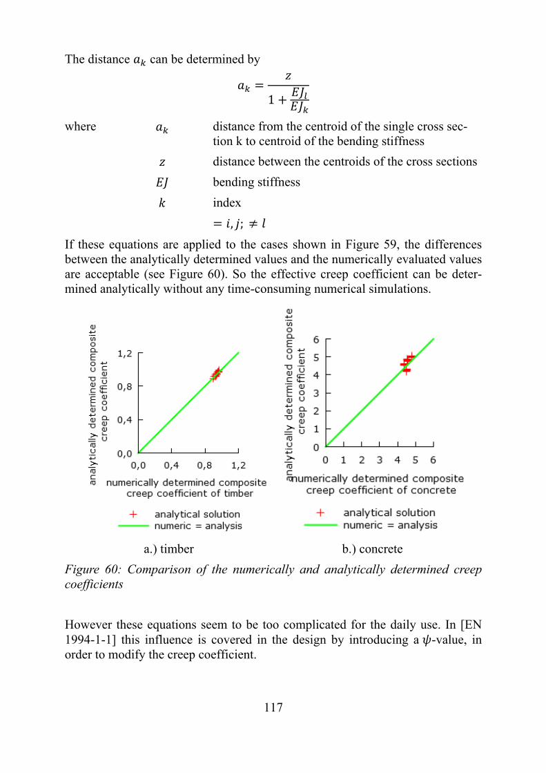
117
The distance can be determined by
1
where distance from the centroid of the single cross sec-tion k to centroid of the bending stiffness
distance between the centroids of the cross sections
bending stiffness
index
, ;
If these equations are applied to the cases shown in Figure 59, the differences between the analytically determined values and the numerically evaluated values are acceptable (see Figure 60). So the effective creep coefficient can be deter-mined analytically without any time-consuming numerical simulations.
a.) timber b.) concrete
Figure 60: Comparison of the numerically and analytically determined creep coefficients
However these equations seem to be too complicated for the daily use. In [EN 1994-1-1] this influence is covered in the design by introducing a -value, in order to modify the creep coefficient.
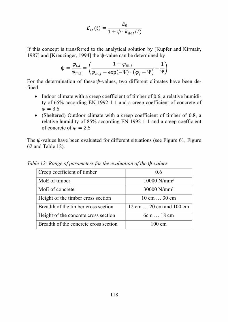
118
1 ⋅
If this concept is transferred to the analytical solution by [Kupfer and Kirmair, 1987] and [Kreuzinger, 1994] the ψ-value can be determined by
ψ ,
,
1 ,
, exp Ψ ⋅ Ψ
1Ψ
For the determination of these -values, two different climates have been de-fined
Indoor climate with a creep coefficient of timber of 0.6, a relative humidi-ty of 65% according EN 1992-1-1 and a creep coefficient of concrete of
3.5 (Sheltered) Outdoor climate with a creep coefficient of timber of 0.8, a
relative humidity of 85% according EN 1992-1-1 and a creep coefficient of concrete of 2.5
The -values have been evaluated for different situations (see Figure 61, Figure 62 and Table 12).
Table 12: Range of parameters for the evaluation of the -values
Creep coefficient of timber 0.6
MoE of timber 10000 N/mm²
MoE of concrete 30000 N/mm²
Height of the timber cross section 10 cm … 30 cm
Breadth of the timber cross section 12 cm … 20 cm and 100 cm
Height of the concrete cross section 6cm … 18 cm
Breadth of the concrete cross section 100 cm
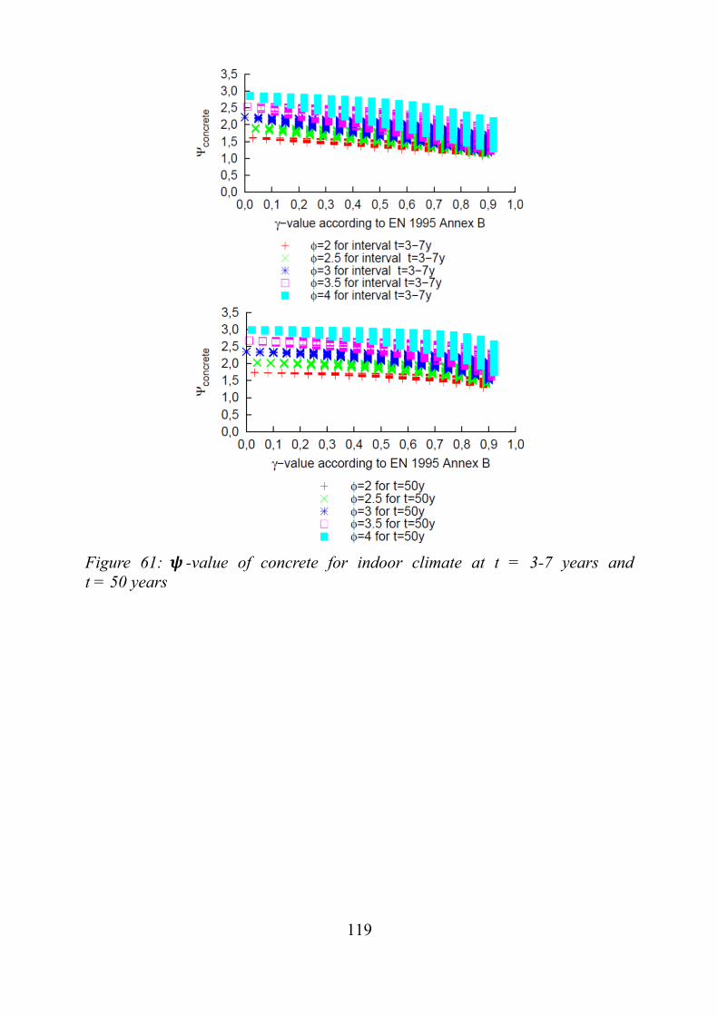
119
Figure 61: -value of concrete for indoor climate at t = 3-7 years and t = 50 years
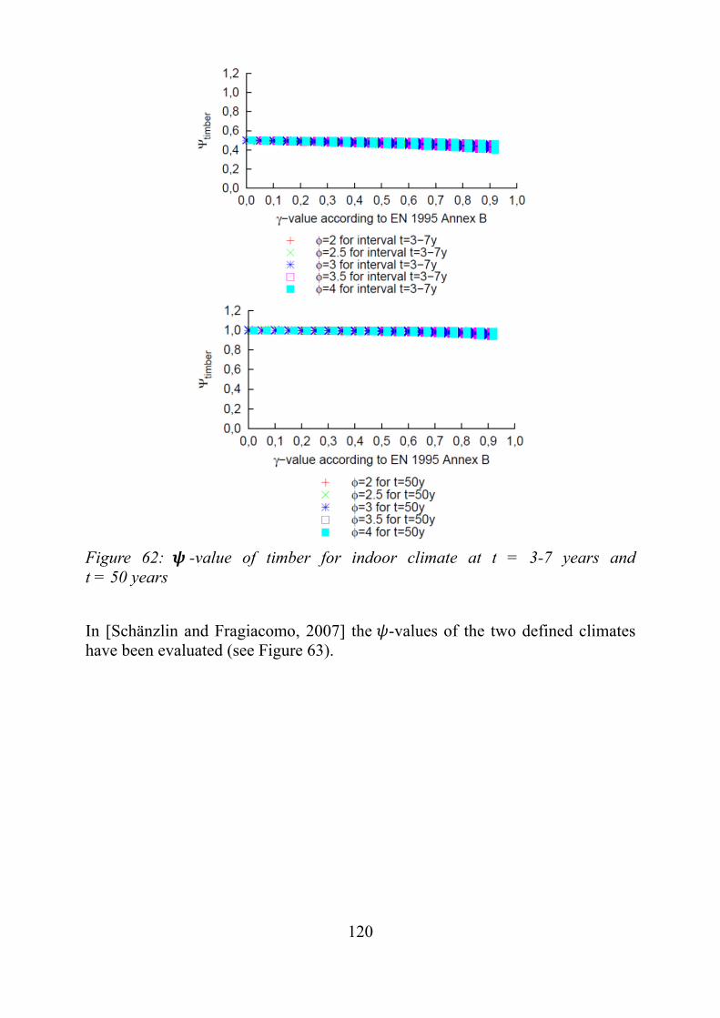
120
Figure 62: -value of timber for indoor climate at t = 3-7 years and t = 50 years
In [Schänzlin and Fragiacomo, 2007] the -values of the two defined climates have been evaluated (see Figure 63).
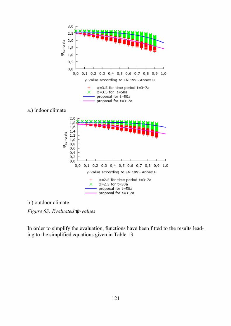
121
a.) indoor climate
b.) outdoor climate
Figure 63: Evaluated -values
In order to simplify the evaluation, functions have been fitted to the results lead-ing to the simplified equations given in Table 13.
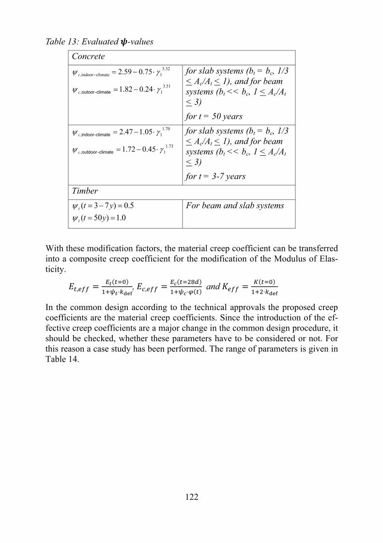
122
Table 13: Evaluated -values
Concrete 32.3
1climateindoor, 75.059.2 c
51.31, 24.082.1 climate-outoorc
for slab systems (bt = bc, 1/3 < Ac/At < 1), and for beam systems (bt << bc, 1 < Ac/At < 3)
for t = 50 years 70.1
1, 05.147.2 climate-indoorc
73.11, 45.072.1 climate-outdoorc
for slab systems (bt = bc, 1/3 < Ac/At < 1), and for beam systems (bt << bc, 1 < Ac/At < 3)
for t = 3-7 years
Timber
5.0)73( ytt 0.1)50( ytt
For beam and slab systems
With these modification factors, the material creep coefficient can be transferred into a composite creep coefficient for the modification of the Modulus of Elas-ticity.
, ⋅, , ⋅
and ⋅
In the common design according to the technical approvals the proposed creep coefficients are the material creep coefficients. Since the introduction of the ef-fective creep coefficients are a major change in the common design procedure, it should be checked, whether these parameters have to be considered or not. For this reason a case study has been performed. The range of parameters is given in Table 14.
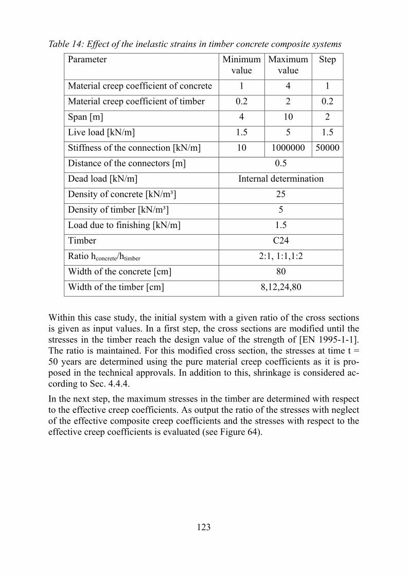
123
Table 14: Effect of the inelastic strains in timber concrete composite systems
Parameter Minimum value
Maximum value
Step
Material creep coefficient of concrete 1 4 1
Material creep coefficient of timber 0.2 2 0.2
Span [m] 4 10 2
Live load [kN/m] 1.5 5 1.5
Stiffness of the connection [kN/m] 10 1000000 50000
Distance of the connectors [m] 0.5
Dead load [kN/m] Internal determination
Density of concrete [kN/m³] 25
Density of timber [kN/m³] 5
Load due to finishing [kN/m] 1.5
Timber C24
Ratio hconcrete/htimber 2:1, 1:1,1:2
Width of the concrete [cm] 80
Width of the timber [cm] 8,12,24,80
Within this case study, the initial system with a given ratio of the cross sections is given as input values. In a first step, the cross sections are modified until the stresses in the timber reach the design value of the strength of [EN 1995-1-1]. The ratio is maintained. For this modified cross section, the stresses at time t = 50 years are determined using the pure material creep coefficients as it is pro-posed in the technical approvals. In addition to this, shrinkage is considered ac-cording to Sec. 4.4.4.
In the next step, the maximum stresses in the timber are determined with respect to the effective creep coefficients. As output the ratio of the stresses with neglect of the effective composite creep coefficients and the stresses with respect to the effective creep coefficients is evaluated (see Figure 64).
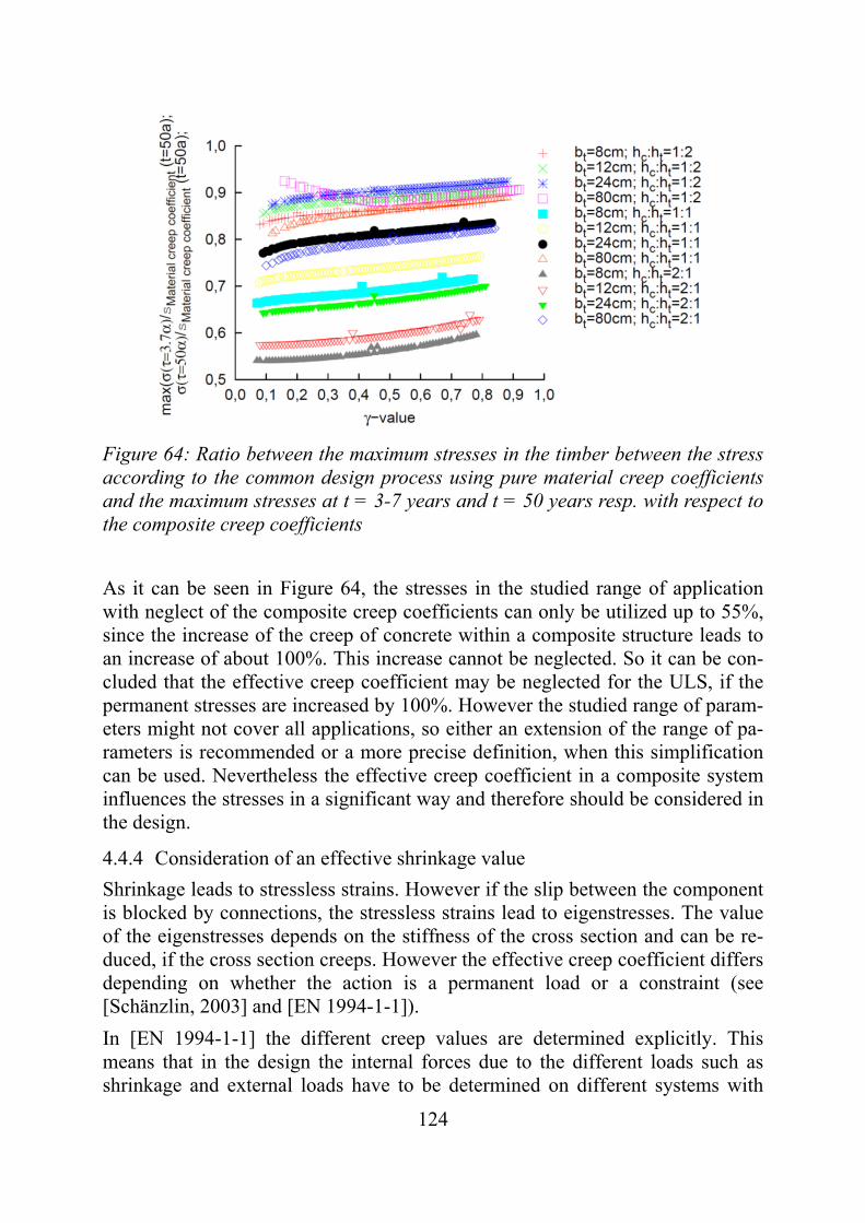
124
Figure 64: Ratio between the maximum stresses in the timber between the stress according to the common design process using pure material creep coefficients and the maximum stresses at t = 3-7 years and t = 50 years resp. with respect to the composite creep coefficients
As it can be seen in Figure 64, the stresses in the studied range of application with neglect of the composite creep coefficients can only be utilized up to 55%, since the increase of the creep of concrete within a composite structure leads to an increase of about 100%. This increase cannot be neglected. So it can be con-cluded that the effective creep coefficient may be neglected for the ULS, if the permanent stresses are increased by 100%. However the studied range of param-eters might not cover all applications, so either an extension of the range of pa-rameters is recommended or a more precise definition, when this simplification can be used. Nevertheless the effective creep coefficient in a composite system influences the stresses in a significant way and therefore should be considered in the design.
4.4.4 Consideration of an effective shrinkage value
Shrinkage leads to stressless strains. However if the slip between the component is blocked by connections, the stressless strains lead to eigenstresses. The value of the eigenstresses depends on the stiffness of the cross section and can be re-duced, if the cross section creeps. However the effective creep coefficient differs depending on whether the action is a permanent load or a constraint (see [Schänzlin, 2003] and [EN 1994-1-1]).
In [EN 1994-1-1] the different creep values are determined explicitly. This means that in the design the internal forces due to the different loads such as shrinkage and external loads have to be determined on different systems with
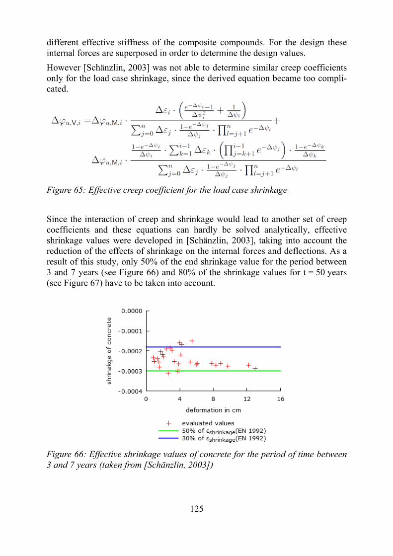
125
different effective stiffness of the composite compounds. For the design these internal forces are superposed in order to determine the design values.
However [Schänzlin, 2003] was not able to determine similar creep coefficients only for the load case shrinkage, since the derived equation became too compli-cated.
Figure 65: Effective creep coefficient for the load case shrinkage
Since the interaction of creep and shrinkage would lead to another set of creep coefficients and these equations can hardly be solved analytically, effective shrinkage values were developed in [Schänzlin, 2003], taking into account the reduction of the effects of shrinkage on the internal forces and deflections. As a result of this study, only 50% of the end shrinkage value for the period between 3 and 7 years (see Figure 66) and 80% of the shrinkage values for t = 50 years (see Figure 67) have to be taken into account.
Figure 66: Effective shrinkage values of concrete for the period of time between 3 and 7 years (taken from [Schänzlin, 2003])
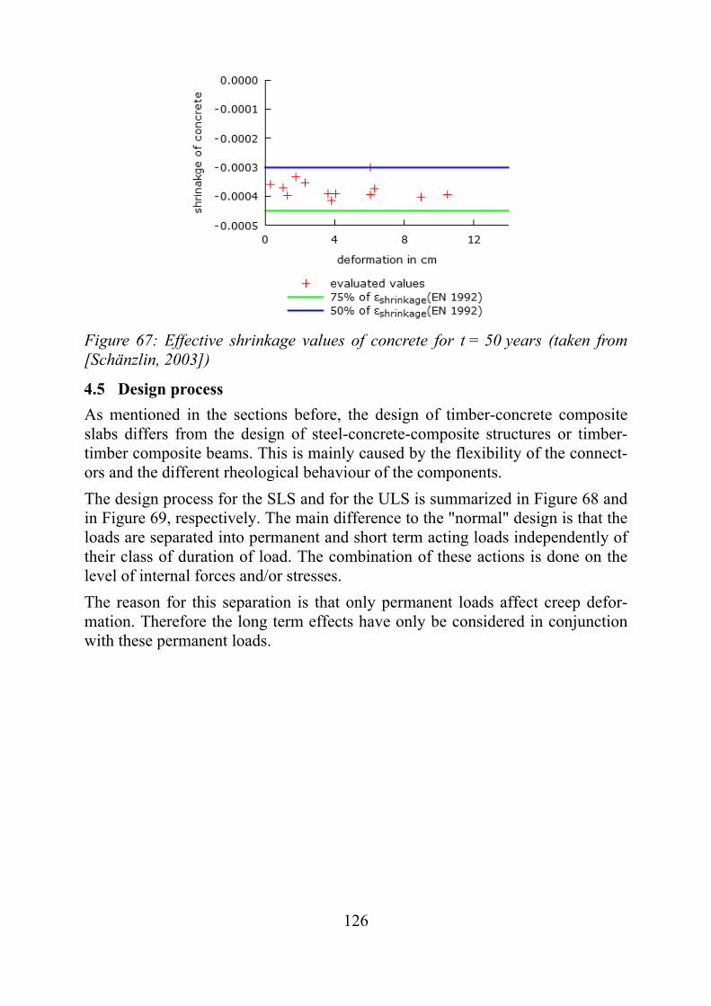
126
Figure 67: Effective shrinkage values of concrete for t = 50 years (taken from [Schänzlin, 2003])
4.5 Design process
As mentioned in the sections before, the design of timber-concrete composite slabs differs from the design of steel-concrete-composite structures or timber-timber composite beams. This is mainly caused by the flexibility of the connect-ors and the different rheological behaviour of the components.
The design process for the SLS and for the ULS is summarized in Figure 68 and in Figure 69, respectively. The main difference to the "normal" design is that the loads are separated into permanent and short term acting loads independently of their class of duration of load. The combination of these actions is done on the level of internal forces and/or stresses.
The reason for this separation is that only permanent loads affect creep defor-mation. Therefore the long term effects have only be considered in conjunction with these permanent loads.
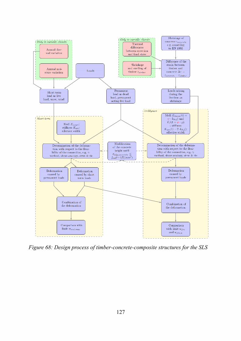
127
Figure 68: Design process of timber-concrete-composite structures for the SLS

128
Figure 69: Design process of timber-concrete-composite structures for the ULS
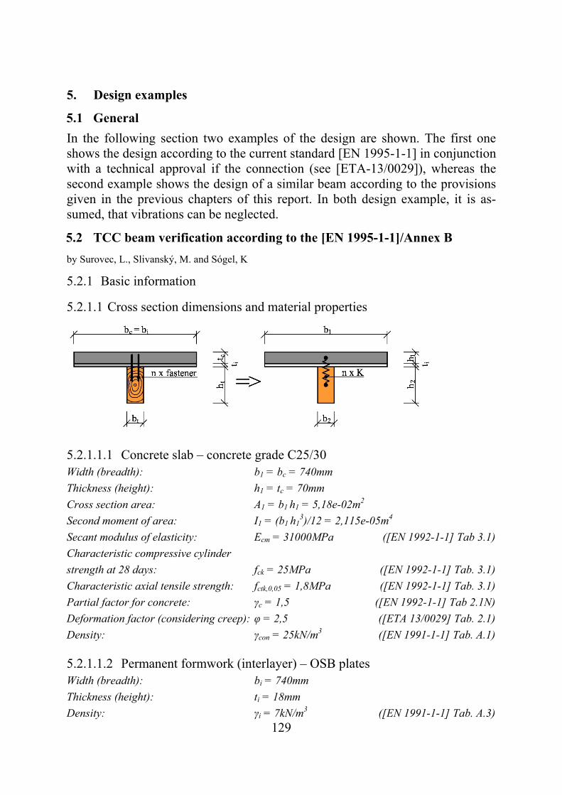
129
5. Design examples
5.1 General
In the following section two examples of the design are shown. The first one shows the design according to the current standard [EN 1995-1-1] in conjunction with a technical approval if the connection (see [ETA-13/0029]), whereas the second example shows the design of a similar beam according to the provisions given in the previous chapters of this report. In both design example, it is as-sumed, that vibrations can be neglected.
5.2 TCC beam verification according to the [EN 1995-1-1]/Annex B
by Surovec, L., Slivanský, M. and Sógel, K
5.2.1 Basic information
5.2.1.1 Cross section dimensions and material properties
5.2.1.1.1 Concrete slab – concrete grade C25/30 Width (breadth): b1 = bc = 740mm
Thickness (height): h1 = tc = 70mm
Cross section area: A1 = b1 h1 = 5,18e-02m2
Second moment of area: I1 = (b1 h13)/12 = 2,115e-05m4
Secant modulus of elasticity: Ecm = 31000MPa ([EN 1992-1-1] Tab 3.1)
Characteristic compressive cylinder
strength at 28 days: fck = 25MPa ([EN 1992-1-1] Tab. 3.1)
Characteristic axial tensile strength: fctk,0,05 = 1,8MPa ([EN 1992-1-1] Tab. 3.1)
Partial factor for concrete: γc = 1,5 ([EN 1992-1-1] Tab 2.1N)
Deformation factor (considering creep): φ = 2,5 ([ETA 13/0029] Tab. 2.1)
Density: γcon = 25kN/m3 ([EN 1991-1-1] Tab. A.1)
5.2.1.1.2 Permanent formwork (interlayer) – OSB plates Width (breadth): bi = 740mm
Thickness (height): ti = 18mm
Density: γi = 7kN/m3 ([EN 1991-1-1] Tab. A.3)
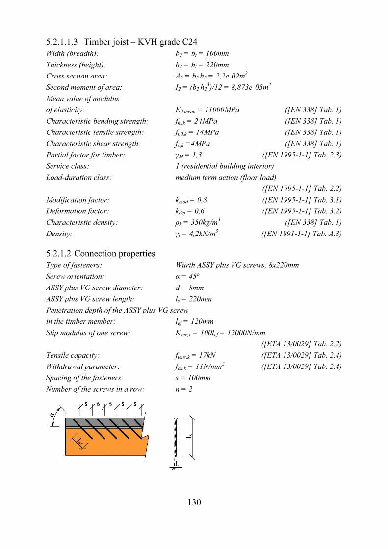
130
5.2.1.1.3 Timber joist – KVH grade C24 Width (breadth): b2 = bt = 100mm
Thickness (height): h2 = ht = 220mm
Cross section area: A2 = b2 h2 = 2,2e-02m2
Second moment of area: I2 = (b2 h23)/12 = 8,873e-05m4
Mean value of modulus
of elasticity: E0,mean = 11000MPa ([EN 338] Tab. 1)
Characteristic bending strength: fm,k = 24MPa ([EN 338] Tab. 1)
Characteristic tensile strength: ft,0,k = 14MPa ([EN 338] Tab. 1)
Characteristic shear strength: fv,k =4MPa ([EN 338] Tab. 1)
Partial factor for timber: γM = 1,3 ([EN 1995-1-1] Tab. 2.3)
Service class: 1 (residential building interior)
Load-duration class: medium term action (floor load)
([EN 1995-1-1] Tab. 2.2)
Modification factor: kmod = 0,8 ([EN 1995-1-1] Tab. 3.1)
Deformation factor: kdef = 0,6 ([EN 1995-1-1] Tab. 3.2)
Characteristic density: ρk = 350kg/m3 ([EN 338] Tab. 1)
Density: γt = 4,2kN/m3 ([EN 1991-1-1] Tab. A.3)
5.2.1.2 Connection properties Type of fasteners: Würth ASSY plus VG screws, 8x220mm
Screw orientation: α = 45°
ASSY plus VG screw diameter: d = 8mm
ASSY plus VG screw length: ls = 220mm
Penetration depth of the ASSY plus VG screw
in the timber member: lef = 120mm
Slip modulus of one screw: Kser,1 = 100lef = 12000N/mm
([ETA 13/0029] Tab. 2.2)
Tensile capacity: ftens,k = 17kN ([ETA 13/0029] Tab. 2.4)
Withdrawal parameter: fax,k = 11N/mm2 ([ETA 13/0029] Tab. 2.4)
Spacing of the fasteners: s = 100mm
Number of the screws in a row: n = 2
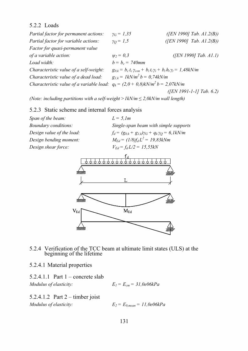
131
5.2.2 Loads
Partial factor for permanent actions: γG = 1,35 ([EN 1990] Tab. A1.2(B))
Partial factor for variable actions: γQ = 1,5 ([EN 1990] Tab. A1.2(B))
Factor for quasi-permanent value
of a variable action: ψ2 = 0,3 ([EN 1990] Tab. A1.1)
Load width: b = bc = 740mm
Characteristic value of a self-weight: g0,k = bc tc γcon + bi ti γi + bt ht γt = 1,48kN/m
Characteristic value of a dead load: g1,k = 1kN/m2 b = 0,74kN/m
Characteristic value of a variable load: qk = (2,0 + 0,8)kN/m2 b = 2,07kN/m
([EN 1991-1-1] Tab. 6.2)
(Note: including partitions with a self-weight >1kN/m ≤ 2,0kN/m wall length)
5.2.3 Static scheme and internal forces analysis
Span of the beam: L = 5,1m
Boundary conditions: Single-span beam with simple supports
Design value of the load: fd = (g0,k + g1,k)γG + qk γQ = 6,1kN/m
Design bending moment: MEd = (1/8)fd L2 = 19,83kNm
Design shear force: VEd = fd L/2 = 15,55kN
5.2.4 Verification of the TCC beam at ultimate limit states (ULS) at the beginning of the lifetime
5.2.4.1 Material properties
5.2.4.1.1 Part 1 – concrete slab Modulus of elasticity: E1 = Ecm = 31,0e06kPa
5.2.4.1.2 Part 2 – timber joist Modulus of elasticity: E2 = E0,mean = 11,0e06kPa
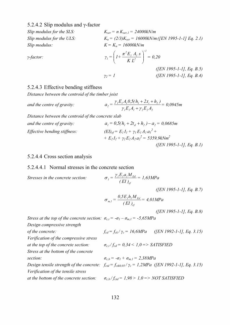
132
5.2.4.2 Slip modulus and γ-factor Slip modulus for the SLS: Kser = n Kser,1 = 24000kN/m
Slip modulus for the ULS: Ku = (2/3)Kser = 16000kN/m ([EN 1995-1-1] Eq. 2.1)
Slip modulus: K = Ku = 16000kN/m
γ-factor:
1
211
2
1 L K
s A Eπ+1=γ
= 0,20
([EN 1995-1-1], Eq. B.5)
γ2 = 1 ([EN 1995-1-1], Eq. B.4)
5.2.4.3 Effective bending stiffness Distance between the centroid of the timber joist
and the centre of gravity: 222111
2i11112 AEAE
)ht.2h(5,0AE=a
= 0,0945m
Distance between the centroid of the concrete slab
and the centre of gravity: 22d11 a)ht2h(5,0=a = 0,0685m
Effective bending stiffness: (EI)ef = E1 I1 + γ1 E1 A1 a12 +
+ E2 I2 + γ2 E2 A2 a22 = 5359,9kNm2
([EN 1995-1-1], Eq. B.1)
5.2.4.4 Cross section analysis
5.2.4.4.1 Normal stresses in the concrete section
Stresses in the concrete section: ef
Ed1111 )EI(
MaE=
= 1,63MPa
([EN 1995-1-1], Eq. B.7)
ef
Ed11m,1 )EI(
MhE5,0= = 4,01MPa
([EN 1995-1-1], Eq. B.8)
Stress at the top of the concrete section: σc,t = -σ1 – σm,1 = -5,65MPa
Design compressive strength
of the concrete: fcd = fck / γc = 16,6MPa ([EN 1992-1-1], Eq. 3.15)
Verification of the compressive stress
at the top of the concrete section: σc,t / fcd = 0,34 < 1,0 => SATISFIED
Stress at the bottom of the concrete
section: σc,b = -σ1 + σm,1 = 2,38MPa
Design tensile strength of the concrete: fctd = fctk0,05 / γc = 1,2MPa ([EN 1992-1-1], Eq. 3.15)
Verification of the tensile stress
at the bottom of the concrete section: σc,b / fctd = 1,98 > 1,0 => NOT SATISFIED
133
5.2.4.4.2 Normal stresses in the timber section
Stresses in the timber section: ef
Ed2222 )EI(
MaE=
= 3,85MPa
([EN 1995-1-1], Eq. B.7)
ef
Ed22m,2 )EI(
MhE5,0= = 4,48MPa
([EN 1995-1-1], Eq. B.8)
Stress at the top of the timber section: σt,t = σ2 – σm,2 = -0,63MPa
Stress at the bottom of the timber
section: σt,b = σ2 + σm,2 = 8,32MPa
Design bending strength of the timber: fm,d = kmod fm,k / γM = 14,76MPa
([EN 1995-1-1], Eq. 2.14)
Design tensile strength of the timber: ft,0,d = kmod ft,0,k / γM = 8,61MPa
([EN 1995-1-1], Eq. 2.14)
Verification of the timber section: σ2 / ft,0,d + σm,2 / fm,d =
= 0,75 < 1,0 => SATISFIED
([EN 1995-1-1], Eq. 6.17)
5.2.4.4.3 Shear stresses in the timber section Height h: h = 0,5h2 + a2 = 0,2045m
Maximal shear stress: Edef
22
max,2 V)EI(
hE5,0 = 0,667MPa
Design shear strength of the timber: fv,d = kmod fv,k / γM = 2,46MPa
([EN 1995-1-1], Eq. 2.14)
Verification of the timber section: τ2,max / fv,d =
= 0,27 < 1,0 => SATISFIED
([EN 1995-1-1], Eq. 6.13)
5.2.4.4.4 Verification of the fasteners
Load on the fasteners in a row: Edef
11111 V
)EI(
saAEF
= 6,64kN
([EN 1995-1-1],Eq. B.10)
Characteristic withdrawal capacity: 8,0
k22
efk,axRk,,ax 350sincos2,1
dlfF
=
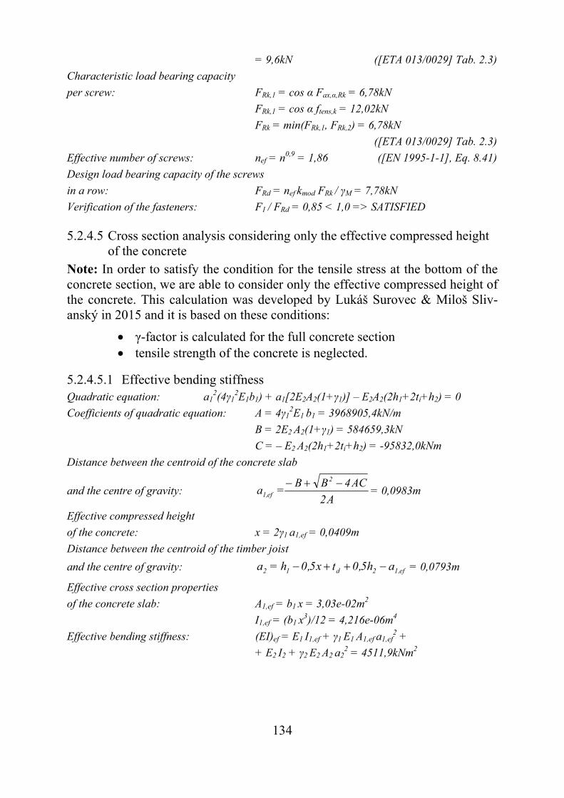
134
= 9,6kN ([ETA 013/0029] Tab. 2.3)
Characteristic load bearing capacity
per screw: FRk,1 = cos α Fax,α,Rk = 6,78kN
FRk,1 = cos α ftens,k = 12,02kN
FRk = min(FRk,1, FRk,2) = 6,78kN
([ETA 013/0029] Tab. 2.3)
Effective number of screws: nef = n0,9 = 1,86 ([EN 1995-1-1], Eq. 8.41)
Design load bearing capacity of the screws
in a row: FRd = nef kmod FRk / γM = 7,78kN
Verification of the fasteners: F1 / FRd = 0,85 < 1,0 => SATISFIED
5.2.4.5 Cross section analysis considering only the effective compressed height of the concrete
Note: In order to satisfy the condition for the tensile stress at the bottom of the concrete section, we are able to consider only the effective compressed height of the concrete. This calculation was developed by Lukáš Surovec & Miloš Sliv-anský in 2015 and it is based on these conditions:
γ-factor is calculated for the full concrete section tensile strength of the concrete is neglected.
5.2.4.5.1 Effective bending stiffness Quadratic equation: a1
2(4γ12E1b1) + a1[2E2A2(1+γ1)] – E2A2(2h1+2ti+h2) = 0
Coefficients of quadratic equation: A = 4γ12E1 b1 = 3968905,4kN/m
B = 2E2 A2(1+γ1) = 584659,3kN
C = – E2 A2(2h1+2ti+h2) = -95832,0kNm
Distance between the centroid of the concrete slab
and the centre of gravity: A2
AC4BB=a
2
ef1,
= 0,0983m
Effective compressed height
of the concrete: x = 2γ1 a1,ef = 0,0409m
Distance between the centroid of the timber joist
and the centre of gravity: ef,12d12 ah5,0tx5,0h=a = 0,0793m
Effective cross section properties
of the concrete slab: A1,ef = b1 x = 3,03e-02m2
I1,ef = (b1 x3)/12 = 4,216e-06m4
Effective bending stiffness: (EI)ef = E1 I1,ef + γ1 E1 A1,ef a1,ef2 +
+ E2 I2 + γ2 E2 A2 a22 = 4511,9kNm2
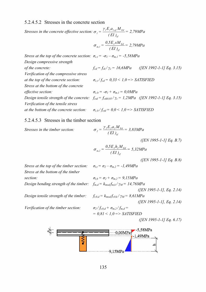
135
5.2.4.5.2 Stresses in the concrete section
Stresses in the concrete effective section: ef
Edef,1111 )EI(
MaE=
= 2,79MPa
ef
Ed1m,1 )EI(
xME5,0= = 2,79MPa
Stress at the top of the concrete section: σc,t = -σ1 – σm,1 = -5,58MPa
Design compressive strength
of the concrete: fcd = fck / γc = 16,6MPa ([EN 1992-1-1] Eq. 3.15)
Verification of the compressive stress
at the top of the concrete section: σc,t / fcd = 0,33 < 1,0 => SATISFIED
Stress at the bottom of the concrete
effective section: σc,b = -σ1 + σm,1 = 0,0MPa
Design tensile strength of the concrete: fctd = fctk0,05 / γc = 1,2MPa ([EN 1992-1-1] Eq. 3.15)
Verification of the tensile stress
at the bottom of the concrete section: σc,b / fctd = 0,0 < 1,0 => SATISFIED
5.2.4.5.3 Stresses in the timber section
Stresses in the timber section: ef
Ed2222 )EI(
MaE=
= 3,83MPa
([EN 1995-1-1] Eq. B.7)
ef
Ed22m,2 )EI(
MhE5,0= = 5,32MPa
([EN 1995-1-1] Eq. B.8)
Stress at the top of the timber section: σt,t = σ2 – σm,2 = -1,49MPa
Stress at the bottom of the timber
section: σt,b = σ2 + σm,2 = 9,15MPa
Design bending strength of the timber: fm,d = kmod fm,k / γM = 14,76MPa
([EN 1995-1-1], Eq. 2.14)
Design tensile strength of the timber: ft,0,d = kmod ft,0,k / γM = 8,61MPa
([EN 1995-1-1], Eq. 2.14)
Verification of the timber section: σ2 / ft,0,d + σm,2 / fm,d =
= 0,81 < 1,0 => SATISFIED
([EN 1995-1-1] Eq. 6.17)
136
5.2.4.5.4 Shear stresses in the timber section Height h: h = 0,5h2 + a2 = 0,1893m
Maximum shear stress: Edef
22
max,2 V)EI(
hE5,0 = 0,679MPa
Design shear strength of the timber: fv,d = kmod fv,k / γM = 2,46MPa
([EN 1995-1-1], Eq. 2.14)
Verification of the timber section: τ2,max / fv,d =
= 0,28 < 1,0 => SATISFIED
([EN 1995-1-1] Eq. 6.13)
5.2.4.5.5 Verification of the fasteners
Load on the fasteners in a row: Edef
ef,1ef,1111 V
)EI(
saAEF
= 6,62kN
([EN 1995-1-1], Eq. B.10)
Characteristic withdrawal capacity: 8,0
k22
efk,axRk,,ax 350sincos2,1
dlfF
=
= 9,6kN
([ETA 13/0029], Tab. 2.3)
Characteristic load bearing capacity
per screw: FRk,1 = cos α Fax,α,Rk = 6,78kN
FRk,1 = cos α ftens,k = 12,02kN
FRk = min(FRk,1, FRk,2) = 6,78kN
([ETA 13/0029], Tab. 2.3)
Effective number of screws: nef = n0,9 = 1,86 ([EN 1995-1-1], Eq. 8.41)
Design load bearing capacity of the screws
in a row: FRd = nef kmod FRk / γM = 7,78kN
Verification of the fasteners: F1 / FRd = 0,85 < 1,0 => SATISFIED
5.2.5 Verification of the TCC beam at ultimate limit states (ULS) at the end of the lifetime
5.2.5.1 Material properties
5.2.5.1.1 Part 1 – concrete slab Modulus of elasticity: E1,g = Ecm / (1+φ)= 8,86e06kPa
E1,q = Ecm / (1+ψ2 φ)= 17,71e06kPa
QkGk,1k,0
Qkq,1Gk,1k,0g,11 q)gg(
qE)gg(EE
= 13,54e03MPa
137
5.2.5.1.2 Part 2 – timber joist Modulus of elasticity: E2,g = E0,mean / (1+kdef)= 6,88e06kPa
([EN 1995-1-1], Eq. 2.7)
E2,q = E0,mean / (1+ψ2 kdef) =
= 9,32e06kPa ([EN 1995-1-1], Eq. 2.10)
QkGk,1k,0
Qkq,2Gk,1k,0g,22 q)gg(
qE)gg(EE
= 8,17e03MPa
5.2.5.2 Slip modulus and γ-factor Slip modulus for the SLS: Kser,g = n Kser,1 / (1 + kdef) =
= 15000kN/m ([EN 1995-1-1], Eq. 2.9)
Kser,q = n Kser,1 / (1 + ψ2 kdef) =
= 20339kN/m ([EN 1995-1-1], Eq. 2.12)
QkGk,1k,0
Qkq,serGk,1k,0g,serser q)gg(
qK)gg(KK
Kser = 17821kN/m
Slip modulus for the ULS: Ku = (2/3)Kser = 11881kN/m
([EN 1995-1-1], Eq. 2.1)
Slip modulus: K = Ku = 11881kN/m
γ-factor:
1
211
2
1 L K
s A Eπ+1=γ
= 0,309
([EN 1995-1-1], Eq. B.5)
γ2 = 1 ([EN 1995-1-1], Eq. B.4)
5.2.5.3 Effective bending stiffness Distance between the centroid of the timber joist
and the centre of gravity: 222111
2i11112 AEAE
)ht.2h(5,0AE=a
= 0,0891m
Distance between the centroid of the concrete slab
and the centre of gravity: 22d11 a)ht2h(5,0=a = 0,0739m
Effective bending stiffness: (EI)ef = E1 I1 + γ1 E1 A1 a12 +
+ E2 I2 + γ2 E2 A2 a22 = 3620,5kNm2
([EN 1995-1-1], Eq. B.1)

138
5.2.5.4 Cross section analysis
5.2.5.4.1 Stresses in the concrete section
Stresses in the concrete section: ef
Ed1111 )EI(
MaE=
= 1,69MPa
([EN 1995-1-1], Eq. B.7)
ef
Ed11m,1 )EI(
MhE5,0= = 2,60MPa
([EN 1995-1-1], Eq. B.8)
Stress at the top of the concrete section: σc,t = -σ1 – σm,1 = -4,29MPa
Design compressive strength
of the concrete: fcd = fck / γc = 16,6MPa ([EN 1992-1-1], Eq. 3.15)
Verification of the compressive stress
at the top of the concrete section: σc,t / fcd = 0,257 < 1,0 => SATISFIED
Stress at the bottom of the concrete
section: σc,b = -σ1 + σm,1 = 0,90MPa
Design tensile strength of the concrete: fctd = fctk0,05 / γc = 1,2MPa ([EN 1992-1-1], Eq. 3.15)
Verification of the tensile stress
at the bottom of the concrete section: σc,b / fctd = 0,75 > 1,0 => NOT SATISFIED
5.2.5.4.2 Stresses in the timber section
Stresses in the timber section: ef
Ed2222 )EI(
MaE=
= 3,99MPa
([EN 1995-1-1], Eq. B.7)
ef
Ed22m,2 )EI(
MhE5,0= = 4,92MPa
([EN 1995-1-1], Eq. B.8)
Stress at the top of the timber section: σt,t = σ2 – σm,2 = -0,94MPa
Stress at the bottom of the timber
section: σt,b = σ2 + σm,2 = 8,91MPa
Design bending strength of the timber: fm,d = kmod fm,k / γM = 14,76MPa
([EN 1995-1-1], Eq. 2.14)
Design tensile strength of the timber: ft,0,d = kmod ft,0,k / γM = 8,61MPa
([EN 1995-1-1], Eq. 2.14)
Verification of the timber section: σ2 / ft,0,d + σm,2 / fm,d =
= 0,80 < 1,0 => SATISFIED
([EN 1995-1-1], Eq. 6.17)
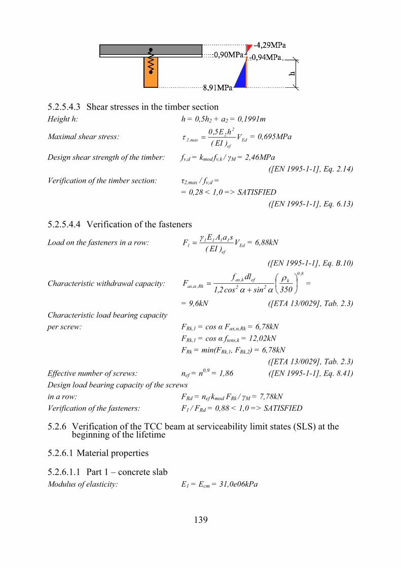
139
5.2.5.4.3 Shear stresses in the timber section Height h: h = 0,5h2 + a2 = 0,1991m
Maximal shear stress: Edef
22
max,2 V)EI(
hE5,0 = 0,695MPa
Design shear strength of the timber: fv,d = kmod fv,k / γM = 2,46MPa
([EN 1995-1-1], Eq. 2.14)
Verification of the timber section: τ2,max / fv,d =
= 0,28 < 1,0 => SATISFIED
([EN 1995-1-1], Eq. 6.13)
5.2.5.4.4 Verification of the fasteners
Load on the fasteners in a row: Edef
11111 V
)EI(
saAEF
= 6,88kN
([EN 1995-1-1], Eq. B.10)
Characteristic withdrawal capacity: 8,0
k22
efk,axRk,,ax 350sincos2,1
dlfF
=
= 9,6kN ([ETA 13/0029], Tab. 2.3)
Characteristic load bearing capacity
per screw: FRk,1 = cos α Fax,α,Rk = 6,78kN
FRk,1 = cos α ftens,k = 12,02kN
FRk = min(FRk,1, FRk,2) = 6,78kN
([ETA 13/0029], Tab. 2.3)
Effective number of screws: nef = n0,9 = 1,86 ([EN 1995-1-1], Eq. 8.41)
Design load bearing capacity of the screws
in a row: FRd = nef kmod FRk / γM = 7,78kN
Verification of the fasteners: F1 / FRd = 0,88 < 1,0 => SATISFIED
5.2.6 Verification of the TCC beam at serviceability limit states (SLS) at the beginning of the lifetime
5.2.6.1 Material properties
5.2.6.1.1 Part 1 – concrete slab Modulus of elasticity: E1 = Ecm = 31,0e06kPa
140
5.2.6.1.2 Part 2 – timber joist Modulus of elasticity: E2 = E0,mean = 11,0e06kPa
5.2.6.2 Slip modulus and γ-factor Slip modulus for the SLS: Kser = n Kser,1 = 24000kN/m
Slip modulus: K = Kser = 24000kN/m
γ-factor:
1
211
2
1 L K
s A Eπ+1=γ
= 0,283
([EN 1995-1-1], Eq. B.5)
γ2 = 1 ([EN 1995-1-1], Eq. B.4)
5.2.6.3 Effective bending stiffness Distance between the centroid of the timber joist
and the centre of gravity: 222111
2i11112 AEAE
)ht.2h(5,0AE=a
= 0,1063m
Distance between the centroid of the concrete slab
and the centre of gravity: 22d11 a)ht2h(5,0=a = 0,0567m
Effective bending stiffness: (EI)ef = E1 I1 + γ1 E1 A1 a12 +
+ E2 I2 + γ2 E2 A2 a22 = 5825,1kNm2
([EN 1995-1-1], Eq. B.1)
5.2.6.4 Deflection at the beginning of the lifetime Characteristic value of the load: fk = g0,k + g1,k + qk = 4,3kN/m
Deflection of the beam: ef
4k
)EI(
Lf
384
5w = 6,5mm
Limit deflection: wlim = L/250 = 20,4mm
Verification of the deflection: w/wlim = 0,32 < 1,0 => SATISFIED
5.2.7 Verification of the TCC beam at serviceability limit states (SLS) at the end of the lifetime
Note: In order to satisfy paragraph 2.2.3 of EN 1995-1-1 it is necessary to calcu-late final deflection by the quasi-permanent load considering creep and instant deflection by the rest of the variable load with no creep.
5.2.7.1 Material properties
5.2.7.1.1 Part 1 – concrete slab Modulus of elasticity: E1,inst = Ecm = 31,0e06kPa
E1,fin = Ecm / (1 + φ) = 8,86e06kPa
141
5.2.7.1.2 Part 2 – timber joist Modulus of elasticity: E2,inst = E0,mean = 11,0e06kPa
E2,fin = E0,mean / (1 + kdef) = 6,88e06kPa
5.2.7.2 Slip modulus and γ-factor Slip modulus for the SLS: Kser,inst = n Kser,1 = 24000kN/m
Kser,fin = n Kser,1 / (1 + kdef) = 15000kN/m
Slip modulus: Kinst = Kser,inst = 24000kN/m
Kfin = Kser = 15000kN/m
γ-factor:
1
2
1inst1,2
inst1,
1
LK
sAEπ+=γ
inst
= 0,283
([EN 1995-1-1], Eq. B.5)
1
2
1fin1,2
fin1,
1
LK
sAEπ+=γ
fin
= 0,463
([EN 1995-1-1], Eq. B.5)
γ2 = 1 ([EN 1995-1-1], Eq. B.4)
5.2.7.3 Effective bending stiffness Distance between the centroid of the timber joist
and the centre of gravity: 2221,1,1
211,1,1inst2,
).2(5,0
AEAE
hthAE=a
instinst
iinstinst
= 0,1063m
2,221,1,1
211,1,1fin2,
).2(5,0
AEAE
hthAE=a
finfinfin
ifinfin
= 0,0952m
Distance between the centroid of the concrete slab
and the centre of gravity: instd ahth=a ,221inst1, )2(5,0 = 0,0567m
find ahth=a ,221fin1, )2(5,0 = 0,0678m
Effective bending stiffness: (EI)ef,inst = E1,inst I1 + γ1,inst E1,inst A1 a1,inst2 + E2,inst I2
+ γ2 E2,inst A2 a2,inst2 = 5825,1kNm2
([EN 1995-1-1], Eq. B.1)
(EI)ef,fin = E1,fin I1 + γ1,fin E1,fin A1 a1,fin2 + E2,fin I2
+ γ2 E2,fin A2 a2,fin2 = 3145,9kNm2
([EN 1995-1-1], Eq. B.1)
5.2.7.4 Deflection at the end of the lifetime Quasi-permanent value of the load: fqp = g0,k + g1,k + ψ2 qk = 2,84kN/m
The rest of the variable load: fq = (1 - ψ2) qk = 1,45kN/m
Deflection of the beam by quasi-permanent load
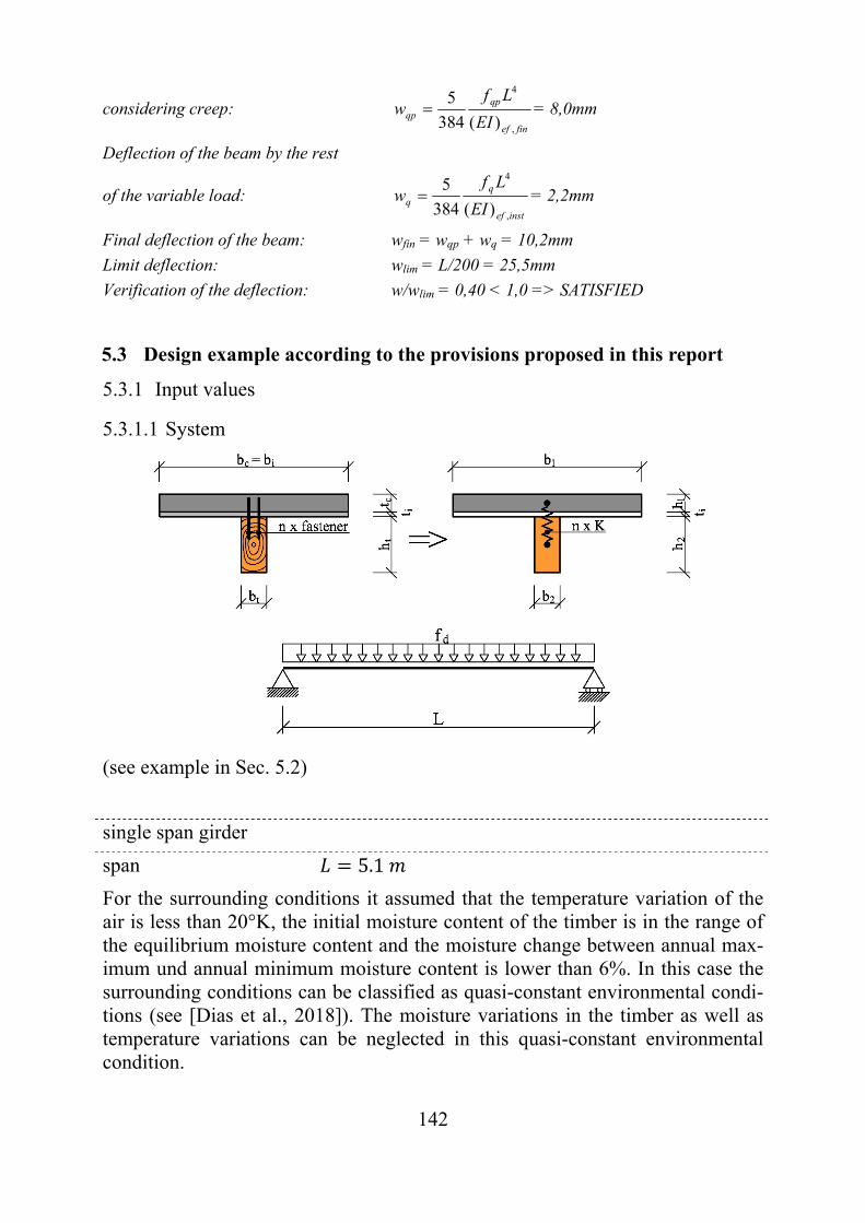
142
considering creep: finef
qpqp EI
Lfw
,
4
)(384
5 = 8,0mm
Deflection of the beam by the rest
of the variable load: instef
qq EI
Lfw
,
4
)(384
5 = 2,2mm
Final deflection of the beam: wfin = wqp + wq = 10,2mm
Limit deflection: wlim = L/200 = 25,5mm
Verification of the deflection: w/wlim = 0,40 < 1,0 => SATISFIED
5.3 Design example according to the provisions proposed in this report
5.3.1 Input values
5.3.1.1 System
(see example in Sec. 5.2)
single span girder
span 5.1
For the surrounding conditions it assumed that the temperature variation of the air is less than 20°K, the initial moisture content of the timber is in the range of the equilibrium moisture content and the moisture change between annual max-imum und annual minimum moisture content is lower than 6%. In this case the surrounding conditions can be classified as quasi-constant environmental condi-tions (see [Dias et al., 2018]). The moisture variations in the timber as well as temperature variations can be neglected in this quasi-constant environmental condition.
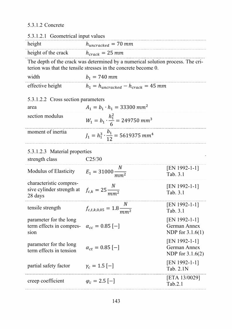
143
5.3.1.2 Concrete
5.3.1.2.1 Geometrical input values
height 70
height of the crack 25
The depth of the crack was determined by a numerical solution process. The cri-terion was that the tensile stresses in the concrete become 0.
width 740
effective height 45
5.3.1.2.2 Cross section parameters
area ∙ 33300
section modulus ∙6
249750
moment of inertia ∙12
5619375
5.3.1.2.3 Material properties
strength class C25/30
Modulus of Elasticity 31000 [EN 1992-1-1] Tab. 3.1
characteristic compres-sive cylinder strength at 28 days
, 25 [EN 1992-1-1] Tab. 3.1
tensile strength , , , , 1.8 [EN 1992-1-1] Tab. 3.1
parameter for the long term effects in compres-sion
0.85 [EN 1992-1-1] German Annex NDP for 3.1.6(1)
parameter for the long term effects in tension
0.85 [EN 1992-1-1] German Annex NDP for 3.1.6(2)
partial safety factor 1.5 [EN 1992-1-1] Tab. 2.1N
creep coefficient 2.5 [ETA 13/0029] Tab.2.1
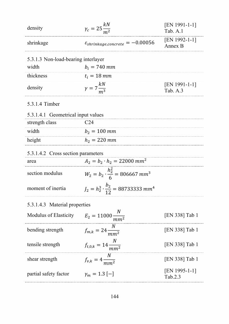
144
density 25 [EN 1991-1-1] Tab. A.1
shrinkage , 0.00056 [EN 1992-1-1] Annex B
5.3.1.3 Non-load-bearing interlayer
width 740
thickness 18
density 7 [EN 1991-1-1] Tab. A.3
5.3.1.4 Timber
5.3.1.4.1 Geometrical input values
strength class C24
width 100
height 220
5.3.1.4.2 Cross section parameters
area ∙ 22000
section modulus ∙6
806667
moment of inertia ∙12
88733333
5.3.1.4.3 Material properties
Modulus of Elasticity 11000 [EN 338] Tab 1
bending strength , 24 [EN 338] Tab 1
tensile strength , , 14 [EN 338] Tab 1
shear strength , 4 [EN 338] Tab 1
partial safety factor 1.3 [EN 1995-1-1] Tab.2.3
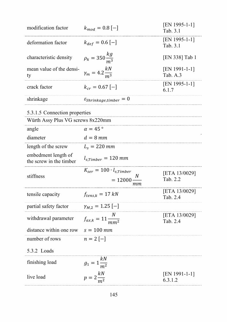
145
modification factor 0.8 [EN 1995-1-1] Tab. 3.1
deformation factor 0.6 [EN 1995-1-1] Tab. 3.1
characteristic density 350 [EN 338] Tab 1
mean value of the densi-ty 4.2
[EN 1991-1-1] Tab. A.3
crack factor 0.67 [EN 1995-1-1] 6.1.7
shrinkage , 0
5.3.1.5 Connection properties
Würth Assy Plus VG screws 8x220mm
angle 45°
diameter 8
length of the screw 220
embedment length of the screw in the timber , 120
stiffness 100 ∙ ,
12000 [ETA 13/0029] Tab. 2.2
tensile capacity , 17 [ETA 13/0029] Tab. 2.4
partial safety factor , 1.25
withdrawal parameter , 11 [ETA 13/0029] Tab. 2.4
distance within one row 100
number of rows 2
5.3.2 Loads
finishing load 1
live load 2 [EN 1991-1-1] 6.3.1.2
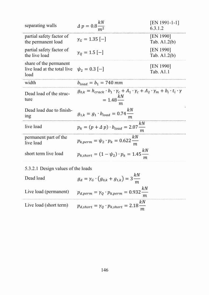
146
separating walls 0.8 [EN 1991-1-1] 6.3.1.2
partial safety factor of the permanent load
1.35 [EN 1990] Tab. A1.2(b)
partial safety factor of the live load
1.5 [EN 1990] Tab. A1.2(b)
share of the permanent live load at the total live load
0.3 [EN 1990] Tab. A1.1
width 740
Dead load of the struc-ture
, ∙ ∙ ∙ ∙ ∙ ∙
1.48
Dead load due to finish-ing , ∙ 0.74
live load ∙ 2.07
permanent part of the live load , ∙ 0.622
short term live load , 1 ∙ 1.45
5.3.2.1 Design values of the loads
Dead load ∙ , , 3
Live load (permanent) , ∙ , 0.932
Live load (short term) , ∙ , 2.18
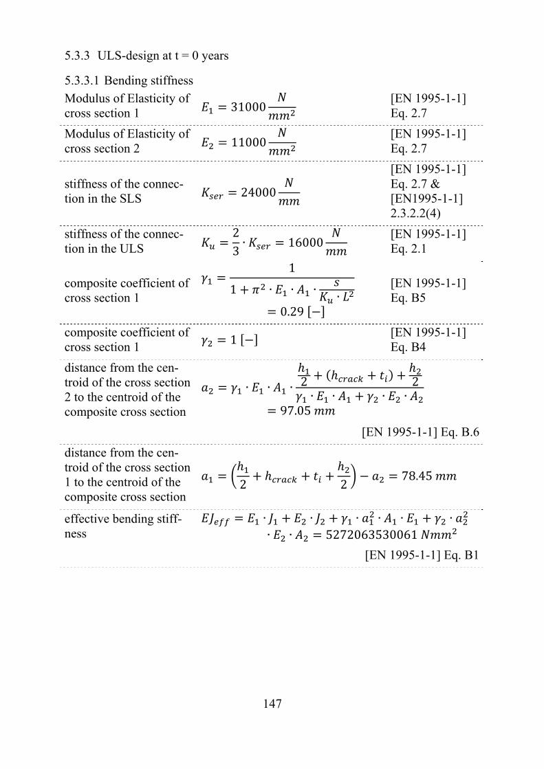
147
5.3.3 ULS-design at t = 0 years
5.3.3.1 Bending stiffness
Modulus of Elasticity of cross section 1 31000
[EN 1995-1-1] Eq. 2.7
Modulus of Elasticity of cross section 2 11000
[EN 1995-1-1] Eq. 2.7
stiffness of the connec-tion in the SLS 24000
[EN 1995-1-1] Eq. 2.7 & [EN1995-1-1] 2.3.2.2(4)
stiffness of the connec-tion in the ULS
23∙ 16000
[EN 1995-1-1] Eq. 2.1
composite coefficient of cross section 1
1
1 ∙ ∙ ∙ ∙0.29
[EN 1995-1-1] Eq. B5
composite coefficient of cross section 1
1 [EN 1995-1-1] Eq. B4
distance from the cen-troid of the cross section 2 to the centroid of the composite cross section
∙ ∙ ∙ 2 2∙ ∙ ∙ ∙
97.05
[EN 1995-1-1] Eq. B.6
distance from the cen-troid of the cross section 1 to the centroid of the composite cross section
2 278.45
effective bending stiff-ness
∙ ∙ ∙ ∙ ∙ ∙∙ ∙ 5272063530061
[EN 1995-1-1] Eq. B1
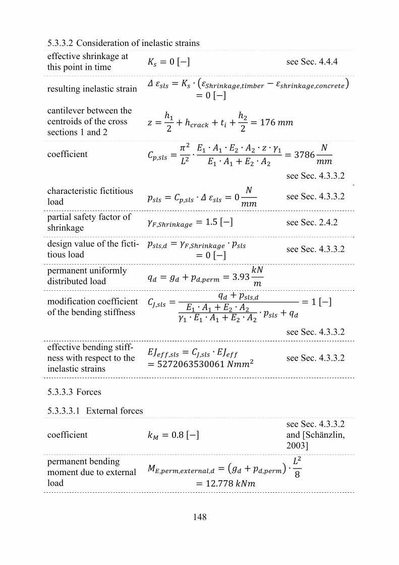
148
5.3.3.2 Consideration of inelastic strains
effective shrinkage at this point in time
0 see Sec. 4.4.4
resulting inelastic strain ∙ , ,
0
cantilever between the centroids of the cross sections 1 and 2 2 2
176
coefficient , ∙∙ ∙ ∙ ∙ ∙∙ ∙
3786
see Sec. 4.3.3.2
characteristic fictitious load , ∙ 0 see Sec. 4.3.3.2
partial safety factor of shrinkage , 1.5 see Sec. 2.4.2
design value of the ficti-tious load
, , ∙0
see Sec. 4.3.3.2
permanent uniformly distributed load , 3.93
modification coefficient of the bending stiffness
,,
∙ ∙∙ ∙ ∙ ∙
1
see Sec. 4.3.3.2
effective bending stiff-ness with respect to the inelastic strains
, , ∙5272063530061
see Sec. 4.3.3.2
5.3.3.3 Forces
5.3.3.3.1 External forces
coefficient 0.8 see Sec. 4.3.3.2 and [Schänzlin, 2003]
permanent bending moment due to external load
, , , , ∙8
12.778
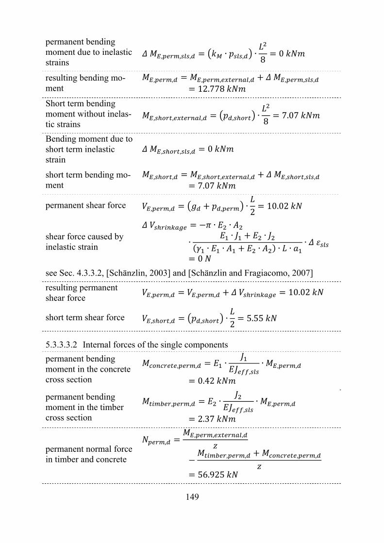
149
permanent bending moment due to inelastic strains
, , , ∙ , ∙8
0
resulting bending mo-ment
, , , , , , , ,
12.778
Short term bending moment without inelas-tic strains
, , , , ∙8
7.07
Bending moment due to short term inelastic strain
, , , 0
short term bending mo-ment
, , , , , , , ,
7.07
permanent shear force , , , ∙2
10.02
shear force caused by inelastic strain
∙ ∙
∙∙ ∙
∙ ∙ ∙ ∙ ∙∙
0
see Sec. 4.3.3.2, [Schänzlin, 2003] and [Schänzlin and Fragiacomo, 2007]
resulting permanent shear force , , , , 10.02
short term shear force , , , ∙2
5.55
5.3.3.3.2 Internal forces of the single components
permanent bending moment in the concrete cross section
, , ∙,
∙ , ,
0.42
permanent bending moment in the timber cross section
, , ∙,
∙ , ,
2.37
permanent normal force in timber and concrete
,, , ,
, , , ,
56.925
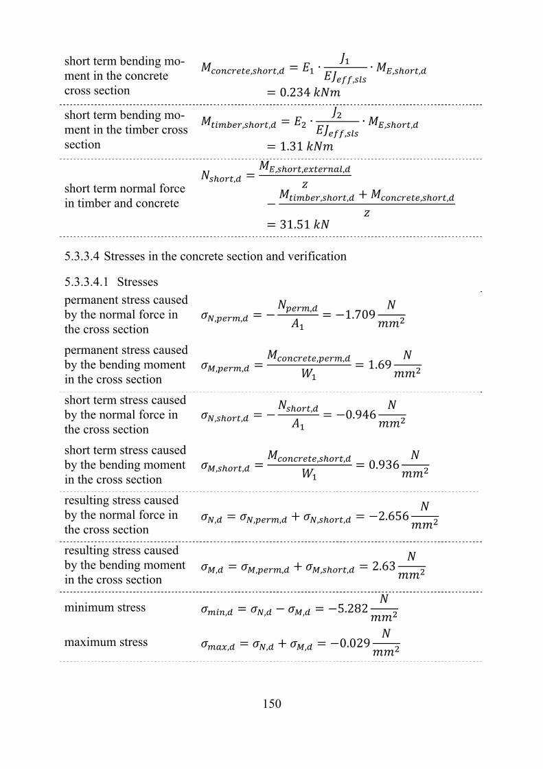
150
short term bending mo-ment in the concrete cross section
, , ∙,
∙ , ,
0.234
short term bending mo-ment in the timber cross section
, , ∙,
∙ , ,
1.31
short term normal force in timber and concrete
,, , ,
, , , ,
31.51
5.3.3.4 Stresses in the concrete section and verification
5.3.3.4.1 Stresses
permanent stress caused by the normal force in the cross section
, ,, 1.709
permanent stress caused by the bending moment in the cross section
, ,, , 1.69
short term stress caused by the normal force in the cross section
, ,, 0.946
short term stress caused by the bending moment in the cross section
, ,, , 0.936
resulting stress caused by the normal force in the cross section
, , , , , 2.656
resulting stress caused by the bending moment in the cross section
, , , , , 2.63
minimum stress , , , 5.282
maximum stress , , , 0.029
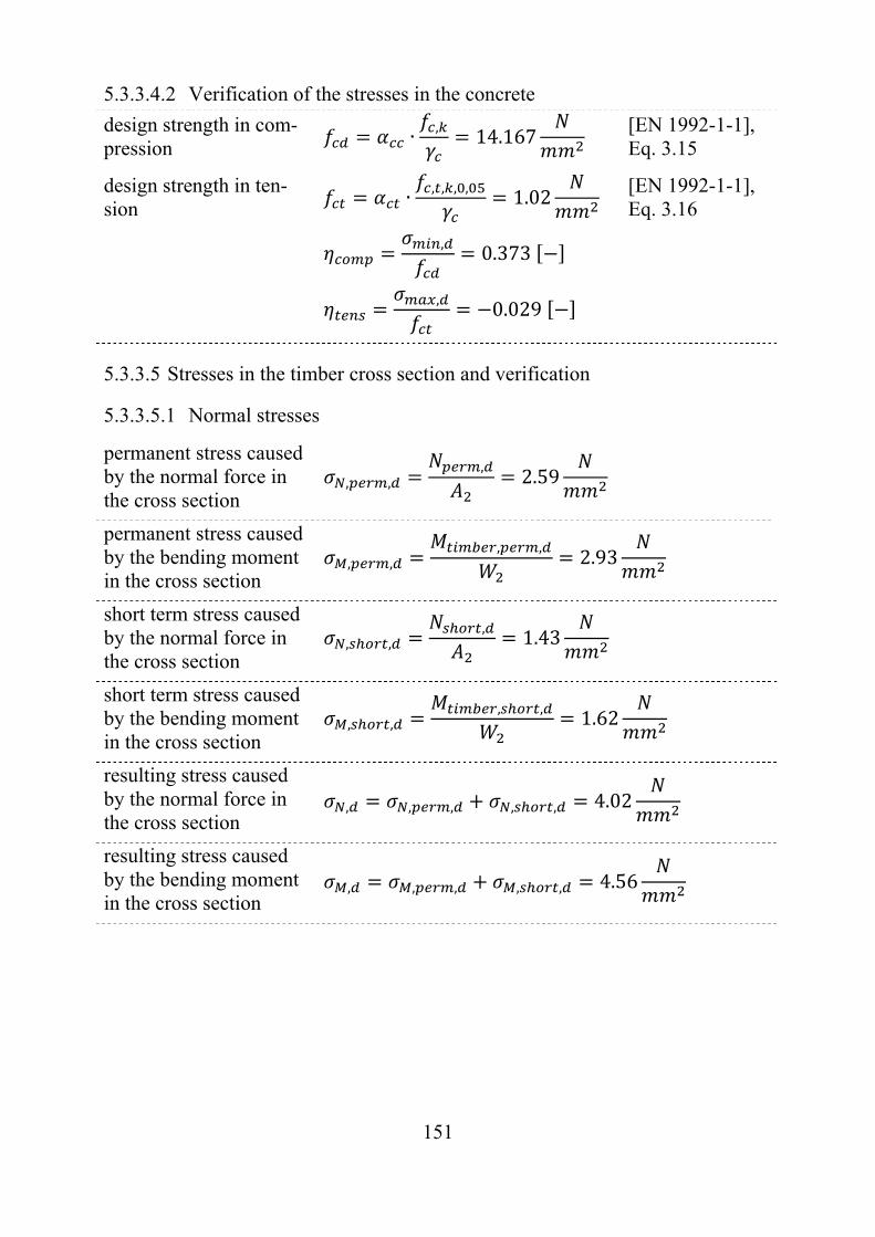
151
5.3.3.4.2 Verification of the stresses in the concrete
design strength in com-pression
∙ , 14.167 [EN 1992-1-1], Eq. 3.15
design strength in ten-sion
∙ , , , , 1.02 [EN 1992-1-1], Eq. 3.16
, 0.373
, 0.029
5.3.3.5 Stresses in the timber cross section and verification
5.3.3.5.1 Normal stresses
permanent stress caused by the normal force in the cross section
, ,, 2.59
permanent stress caused by the bending moment in the cross section
, ,, , 2.93
short term stress caused by the normal force in the cross section
, ,, 1.43
short term stress caused by the bending moment in the cross section
, ,, , 1.62
resulting stress caused by the normal force in the cross section
, , , , , 4.02
resulting stress caused by the bending moment in the cross section
, , , , , 4.56
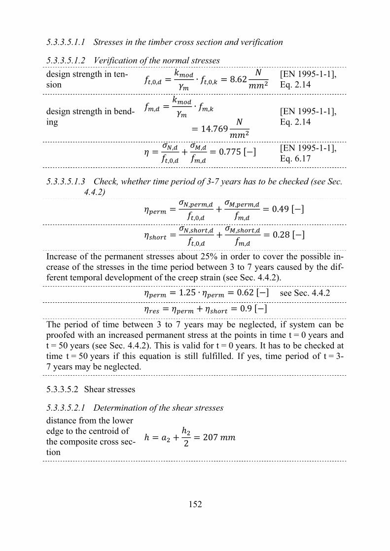
152
5.3.3.5.1.1 Stresses in the timber cross section and verification
5.3.3.5.1.2 Verification of the normal stresses
design strength in ten-sion , , ∙ , , 8.62
[EN 1995-1-1], Eq. 2.14
design strength in bend-ing
, ∙ ,
14.769
[EN 1995-1-1], Eq. 2.14
,
, ,
,
,0.775 [EN 1995-1-1],
Eq. 6.17
5.3.3.5.1.3 Check, whether time period of 3-7 years has to be checked (see Sec. 4.4.2)
, ,
, ,
, ,
,0.49
, ,
, ,
, ,
,0.28
Increase of the permanent stresses about 25% in order to cover the possible in-crease of the stresses in the time period between 3 to 7 years caused by the dif-ferent temporal development of the creep strain (see Sec. 4.4.2).
1.25 ∙ 0.62 see Sec. 4.4.2
0.9
The period of time between 3 to 7 years may be neglected, if system can be proofed with an increased permanent stress at the points in time t = 0 years and t = 50 years (see Sec. 4.4.2). This is valid for t = 0 years. It has to be checked at time t = 50 years if this equation is still fulfilled. If yes, time period of t = 3-7 years may be neglected.
5.3.3.5.2 Shear stresses
5.3.3.5.2.1 Determination of the shear stresses
distance from the lower edge to the centroid of the composite cross sec-tion
2207

153
permanent shear stress , 0.5 ∙ ∙
,∙ , ,
0.669
[EN 1995-1-1], B.9
short term shear stress , 0.5 ∙ ∙,
∙ , , 0.37
[EN 1995-1-1], B.9
resulting shear stress , , , 1.04
5.3.3.5.2.2 Verification of the shear
design strength in shear , ∙ , 2.46 [EN 1995-1-1], Eq. 2.14
,
,0.42 [EN 1995-1-1],
Eq. 6.13
5.3.3.6 Connection
5.3.3.6.1 Forces in the connection
permanent force in the connection
, , ∙ ∙ ∙ ∙,
∙ , ,
4465
[EN 1995-1-1], Eq. B.10
short term force in the connection
, , ∙ ∙ ∙ ∙,
∙ , ,
2471
[EN 1995-1-1], Eq. B.10
resulting force in the connection , , , , 6936
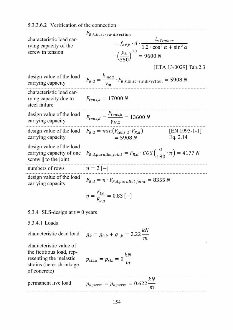
154
5.3.3.6.2 Verification of the connection
characteristic load car-rying capacity of the screw in tension
, ,
, ∙ ∙ ,
1.2 ∙ cos sin
∙350
.9600
[ETA 13/0029] Tab.2.3
design value of the load carrying capacity , ∙ , , 5908
characteristic load car-rying capacity due to steel failure
, 17000
design value of the load carrying capacity ,
,
,13600
design value of the load carrying capacity
, , ; ,
5908 [EN 1995-1-1] Eq. 2.14
design value of the load carrying capacity of one screw || to the joint
, , , ∙180
∙ 4177
numbers of rows 2
design value of the load carrying capacity , ∙ , , 8355
,
0.83
5.3.4 SLS-design at t = 0 years
5.3.4.1 Loads
characteristic dead load , , 2.22
characteristic value of the fictitious load, rep-resenting the inelastic strains (here: shrinkage of concrete)
, 0
permanent live load , , 0.622
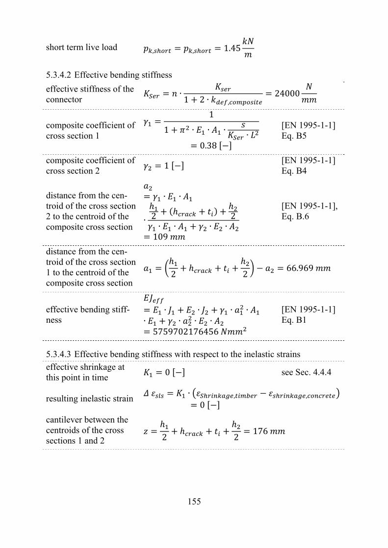
155
short term live load , , 1.45
5.3.4.2 Effective bending stiffness
effective stiffness of the connector
∙1 2 ∙ ,
24000
composite coefficient of cross section 1
1
1 ∙ ∙ ∙ ∙0.38
[EN 1995-1-1] Eq. B5
composite coefficient of cross section 2
1 [EN 1995-1-1] Eq. B4
distance from the cen-troid of the cross section 2 to the centroid of the composite cross section
∙ ∙
∙ 2 2∙ ∙ ∙ ∙109
[EN 1995-1-1], Eq. B.6
distance from the cen-troid of the cross section 1 to the centroid of the composite cross section
2 266.969
effective bending stiff-ness
∙ ∙ ∙ ∙∙ ∙ ∙ ∙5759702176456
[EN 1995-1-1] Eq. B1
5.3.4.3 Effective bending stiffness with respect to the inelastic strains
effective shrinkage at this point in time
0 see Sec. 4.4.4
resulting inelastic strain ∙ , ,
0
cantilever between the centroids of the cross sections 1 and 2 2 2
176
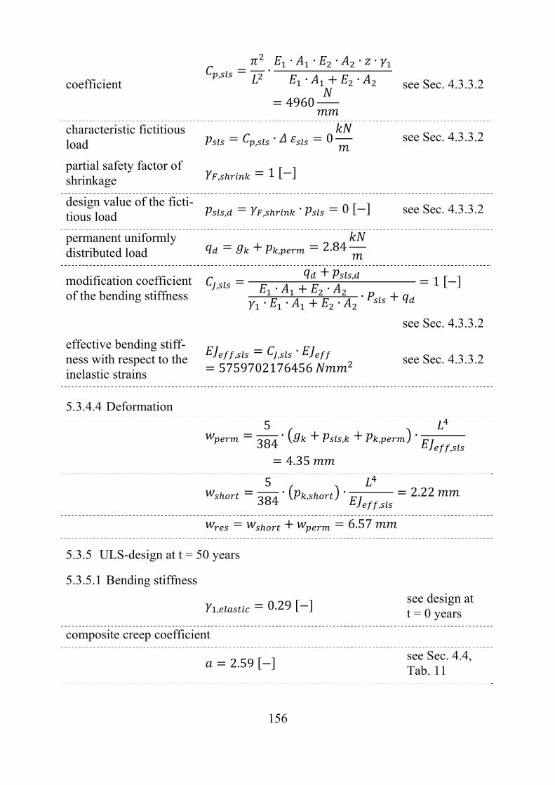
156
coefficient , ∙
∙ ∙ ∙ ∙ ∙∙ ∙
4960
see Sec. 4.3.3.2
characteristic fictitious load , ∙ 0 see Sec. 4.3.3.2
partial safety factor of shrinkage , 1
design value of the ficti-tious load , , ∙ 0 see Sec. 4.3.3.2
permanent uniformly distributed load , 2.84
modification coefficient of the bending stiffness
,,
∙ ∙∙ ∙ ∙ ∙
1
see Sec. 4.3.3.2
effective bending stiff-ness with respect to the inelastic strains
, , ∙5759702176456
see Sec. 4.3.3.2
5.3.4.4 Deformation
5384
∙ , , ∙,
4.35
5384
∙ , ∙,
2.22
6.57
5.3.5 ULS-design at t = 50 years
5.3.5.1 Bending stiffness
, 0.29 see design at t = 0 years
composite creep coefficient
2.59 see Sec. 4.4, Tab. 11
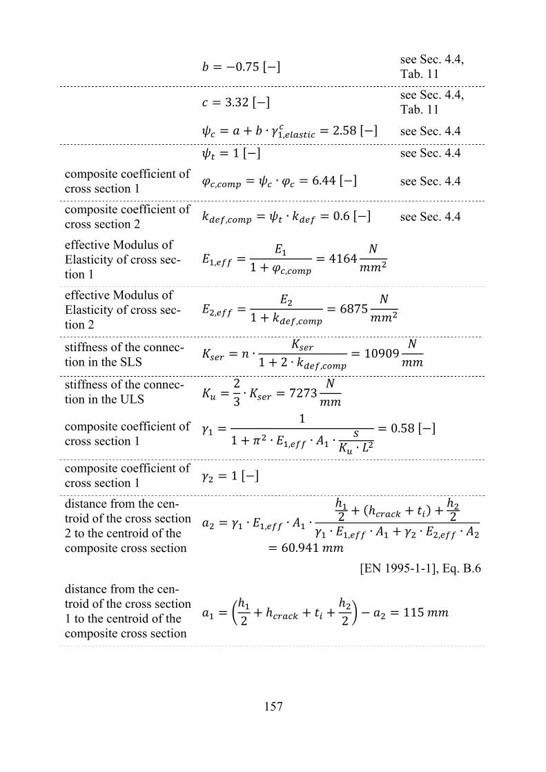
157
0.75 see Sec. 4.4, Tab. 11
3.32 see Sec. 4.4, Tab. 11
∙ , 2.58 see Sec. 4.4
1 see Sec. 4.4
composite coefficient of cross section 1 , ∙ 6.44 see Sec. 4.4
composite coefficient of cross section 2 , ∙ 0.6 see Sec. 4.4
effective Modulus of Elasticity of cross sec-tion 1
, 1 ,4164
effective Modulus of Elasticity of cross sec-tion 2
, 1 ,6875
stiffness of the connec-tion in the SLS
∙1 2 ∙ ,
10909
stiffness of the connec-tion in the ULS
23∙ 7273
composite coefficient of cross section 1
1
1 ∙ , ∙ ∙ ∙
0.58
composite coefficient of cross section 1
1
distance from the cen-troid of the cross section 2 to the centroid of the composite cross section
∙ , ∙ ∙ 2 2∙ , ∙ ∙ , ∙
60.941
[EN 1995-1-1], Eq. B.6
distance from the cen-troid of the cross section 1 to the centroid of the composite cross section
2 2115
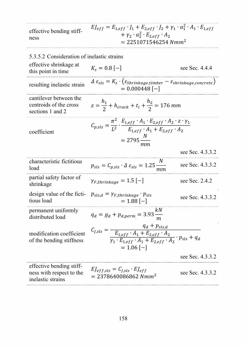
158
effective bending stiff-ness
, ∙ , ∙ ∙ ∙ ∙ ,
∙ ∙ , ∙2251071546254
5.3.5.2 Consideration of inelastic strains
effective shrinkage at this point in time
0.8 see Sec. 4.4.4
resulting inelastic strain ⋅ , ,
0.000448
cantilever between the centroids of the cross sections 1 and 2 2 2
176
coefficient , ∙ , ∙ ∙ , ∙ ∙ ∙
, ∙ , ∙
2795
see Sec. 4.3.3.2
characteristic fictitious load , ∙ 1.25 see Sec. 4.3.3.2
partial safety factor of shrinkage , 1.5 see Sec. 2.4.2
design value of the ficti-tious load
, , ∙1.88
see Sec. 4.3.3.2
permanent uniformly distributed load , 3.93
modification coefficient of the bending stiffness
,,
, ∙ , ∙∙ , ∙ , ∙ ∙
1.06
see Sec. 4.3.3.2
effective bending stiff-ness with respect to the inelastic strains
, , ∙2378640086862
see Sec. 4.3.3.2
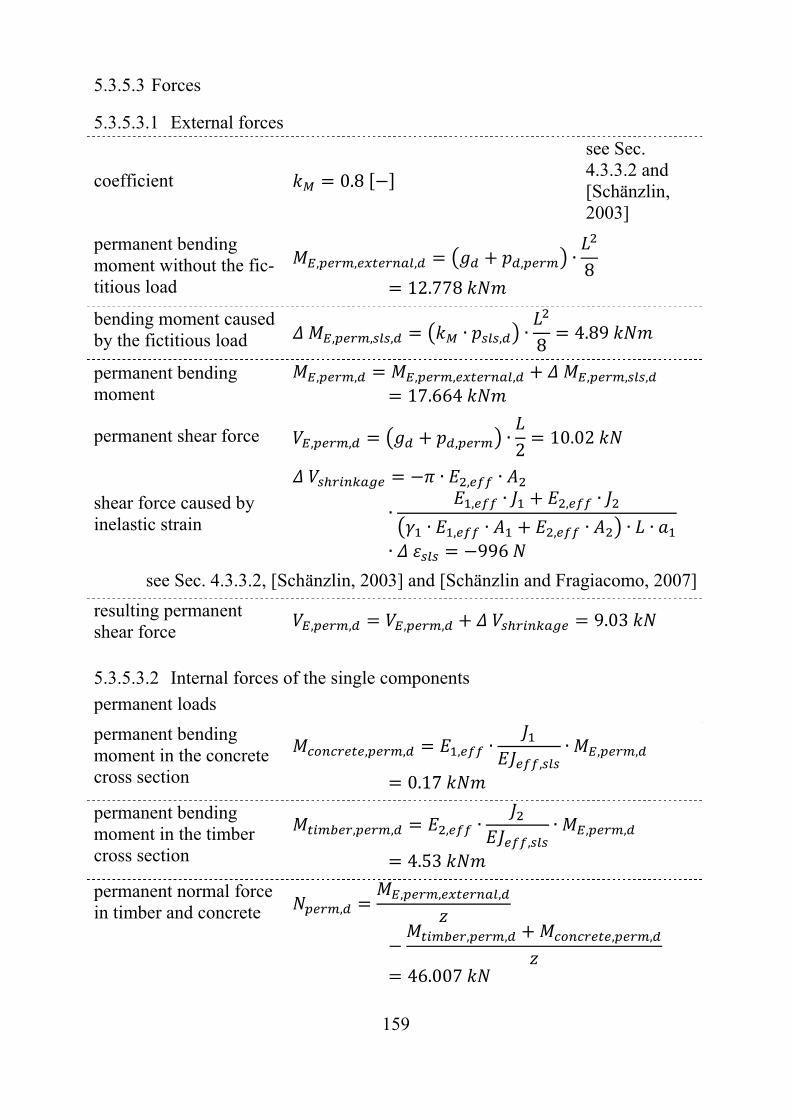
159
5.3.5.3 Forces
5.3.5.3.1 External forces
coefficient 0.8
see Sec. 4.3.3.2 and [Schänzlin, 2003]
permanent bending moment without the fic-titious load
, , , , ∙8
12.778
bending moment caused by the fictitious load , , , ∙ , ∙
84.89
permanent bending moment
, , , , , , , ,
17.664
permanent shear force , , , ∙2
10.02
shear force caused by inelastic strain
∙ , ∙
∙ , ∙ , ∙
∙ , ∙ , ∙ ∙ ∙∙ 996
see Sec. 4.3.3.2, [Schänzlin, 2003] and [Schänzlin and Fragiacomo, 2007]
resulting permanent shear force , , , , 9.03
5.3.5.3.2 Internal forces of the single components
permanent loads
permanent bending moment in the concrete cross section
, , , ∙,
∙ , ,
0.17
permanent bending moment in the timber cross section
, , , ∙,
∙ , ,
4.53
permanent normal force in timber and concrete ,
, , ,
, , , ,
46.007
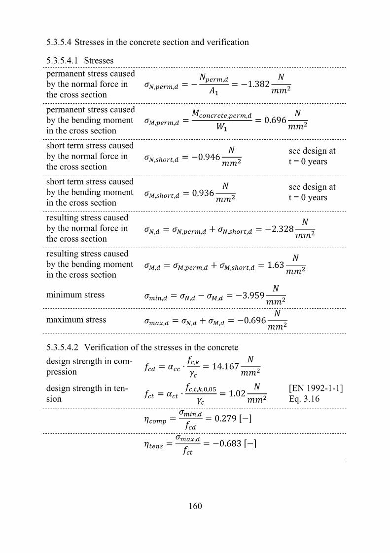
160
5.3.5.4 Stresses in the concrete section and verification
5.3.5.4.1 Stresses
permanent stress caused by the normal force in the cross section
, ,, 1.382
permanent stress caused by the bending moment in the cross section
, ,, , 0.696
short term stress caused by the normal force in the cross section
, , 0.946 see design at t = 0 years
short term stress caused by the bending moment in the cross section
, , 0.936 see design at t = 0 years
resulting stress caused by the normal force in the cross section
, , , , , 2.328
resulting stress caused by the bending moment in the cross section
, , , , , 1.63
minimum stress , , , 3.959
maximum stress , , , 0.696
5.3.5.4.2 Verification of the stresses in the concrete
design strength in com-pression
∙ , 14.167
design strength in ten-sion
∙ , , , , 1.02 [EN 1992-1-1] Eq. 3.16
, 0.279
, 0.683
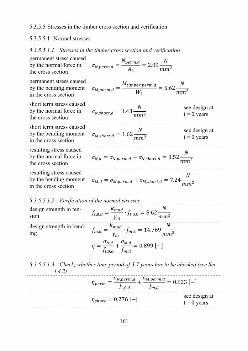
161
5.3.5.5 Stresses in the timber cross section and verification
5.3.5.5.1 Normal stresses
5.3.5.5.1.1 Stresses in the timber cross section and verification
permanent stress caused by the normal force in the cross section
, ,, 2.09
permanent stress caused by the bending moment in the cross section
, ,, , 5.62
short term stress caused by the normal force in the cross section
, , 1.43 see design at t = 0 years
short term stress caused by the bending moment in the cross section
, , 1.62 see design at t = 0 years
resulting stress caused by the normal force in the cross section
, , , , , 3.52
resulting stress caused by the bending moment in the cross section
, , , , , 7.24
5.3.5.5.1.2 Verification of the normal stresses
design strength in ten-sion , , ∙ , , 8.62
design strength in bend-ing , ∙ , 14.769
,
, ,
,
,0.899
5.3.5.5.1.3 Check, whether time period of 3-7 years has to be checked (see Sec. 4.4.2)
, ,
, ,
, ,
,0.623
0.276 see design at t = 0 years
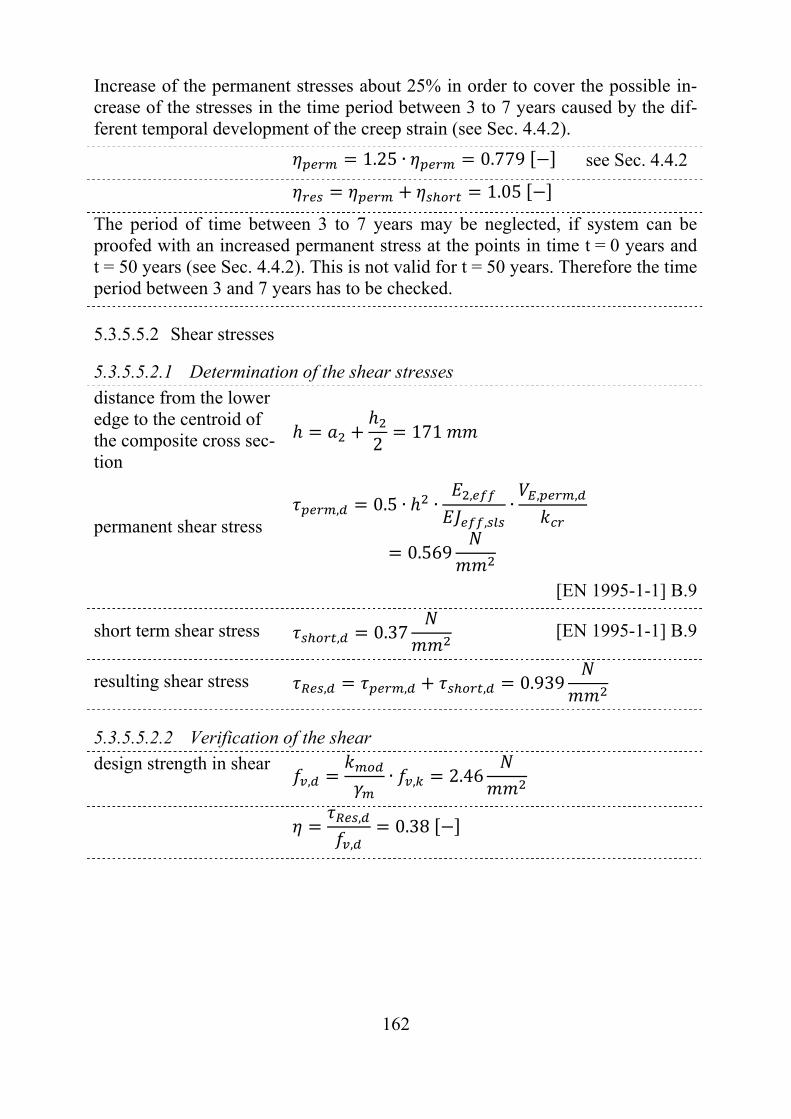
162
Increase of the permanent stresses about 25% in order to cover the possible in-crease of the stresses in the time period between 3 to 7 years caused by the dif-ferent temporal development of the creep strain (see Sec. 4.4.2).
1.25 ∙ 0.779 see Sec. 4.4.2
1.05
The period of time between 3 to 7 years may be neglected, if system can be proofed with an increased permanent stress at the points in time t = 0 years and t = 50 years (see Sec. 4.4.2). This is not valid for t = 50 years. Therefore the time period between 3 and 7 years has to be checked.
5.3.5.5.2 Shear stresses
5.3.5.5.2.1 Determination of the shear stresses
distance from the lower edge to the centroid of the composite cross sec-tion
2171
permanent shear stress , 0.5 ∙ ∙ ,
,∙ , ,
0.569
[EN 1995-1-1] B.9
short term shear stress , 0.37 [EN 1995-1-1] B.9
resulting shear stress , , , 0.939
5.3.5.5.2.2 Verification of the shear
design strength in shear , ∙ , 2.46
,
,0.38
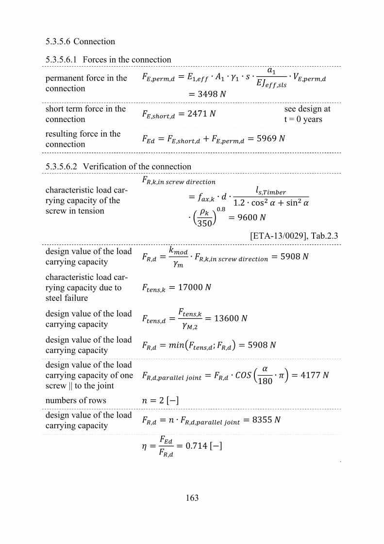
163
5.3.5.6 Connection
5.3.5.6.1 Forces in the connection
permanent force in the connection
, , , ∙ ∙ ∙ ∙,
∙ , ,
3498
short term force in the connection , , 2471 see design at
t = 0 years
resulting force in the connection , , , , 5969
5.3.5.6.2 Verification of the connection
characteristic load car-rying capacity of the screw in tension
, ,
, ∙ ∙ ,
1.2 ∙ cos sin
∙350
.9600
[ETA-13/0029], Tab.2.3
design value of the load carrying capacity , ∙ , , 5908
characteristic load car-rying capacity due to steel failure
, 17000
design value of the load carrying capacity ,
,
,13600
design value of the load carrying capacity , , ; , 5908
design value of the load carrying capacity of one screw || to the joint
, , , ∙180
∙ 4177
numbers of rows 2
design value of the load carrying capacity , ∙ , , 8355
,
0.714
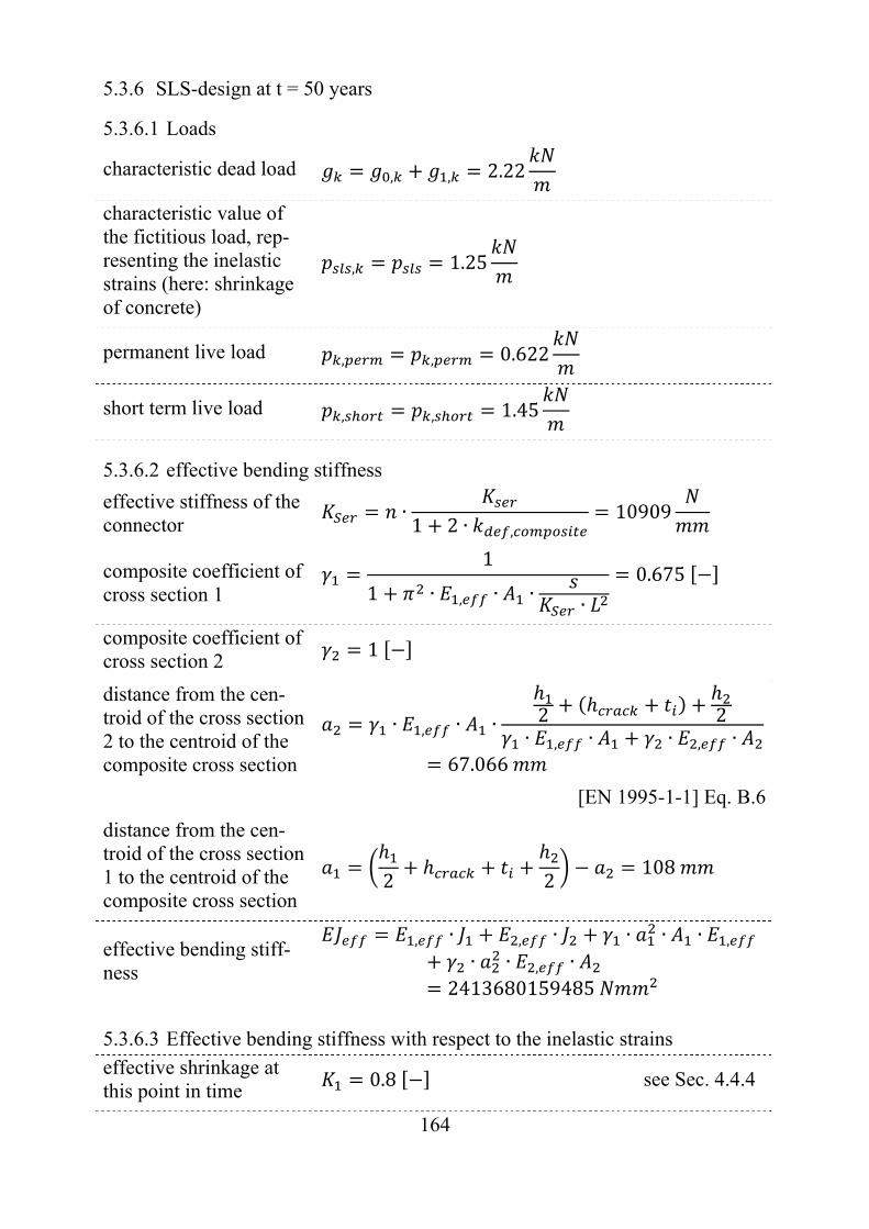
164
5.3.6 SLS-design at t = 50 years
5.3.6.1 Loads
characteristic dead load , , 2.22
characteristic value of the fictitious load, rep-resenting the inelastic strains (here: shrinkage of concrete)
, 1.25
permanent live load , , 0.622
short term live load , , 1.45
5.3.6.2 effective bending stiffness
effective stiffness of the connector
∙1 2 ∙ ,
10909
composite coefficient of cross section 1
1
1 ∙ , ∙ ∙ ∙
0.675
composite coefficient of cross section 2
1
distance from the cen-troid of the cross section 2 to the centroid of the composite cross section
∙ , ∙ ∙ 2 2∙ , ∙ ∙ , ∙
67.066
[EN 1995-1-1] Eq. B.6
distance from the cen-troid of the cross section 1 to the centroid of the composite cross section
2 2108
effective bending stiff-ness
, ∙ , ∙ ∙ ∙ ∙ ,
∙ ∙ , ∙2413680159485
5.3.6.3 Effective bending stiffness with respect to the inelastic strains
effective shrinkage at this point in time
0.8 see Sec. 4.4.4
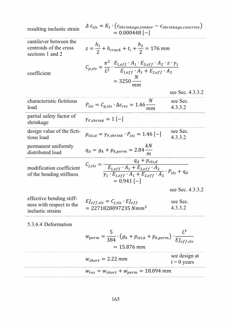
165
resulting inelastic strain ∙ , ,
0.000448
cantilever between the centroids of the cross sections 1 and 2 2 2
176
coefficient , ∙ , ∙ ∙ , ∙ ∙ ∙
, ∙ , ∙
3250
see Sec. 4.3.3.2
characteristic fictitious load , ∙ Δ 1.46
see Sec. 4.3.3.2
partial safety factor of shrinkage , 1
design value of the ficti-tious load , , ∙ 1.46 see Sec.
4.3.3.2
permanent uniformly distributed load , 2.84
modification coefficient of the bending stiffness
,,
, ∙ , ∙∙ , ∙ , ∙ ∙
0.941
see Sec. 4.3.3.2
effective bending stiff-ness with respect to the inelastic strains
, , ∙2271828097235
see Sec. 4.3.3.2
5.3.6.4 Deformation
5384
∙ , , ∙,
15.876
2.22 see design at t = 0 years
18.094
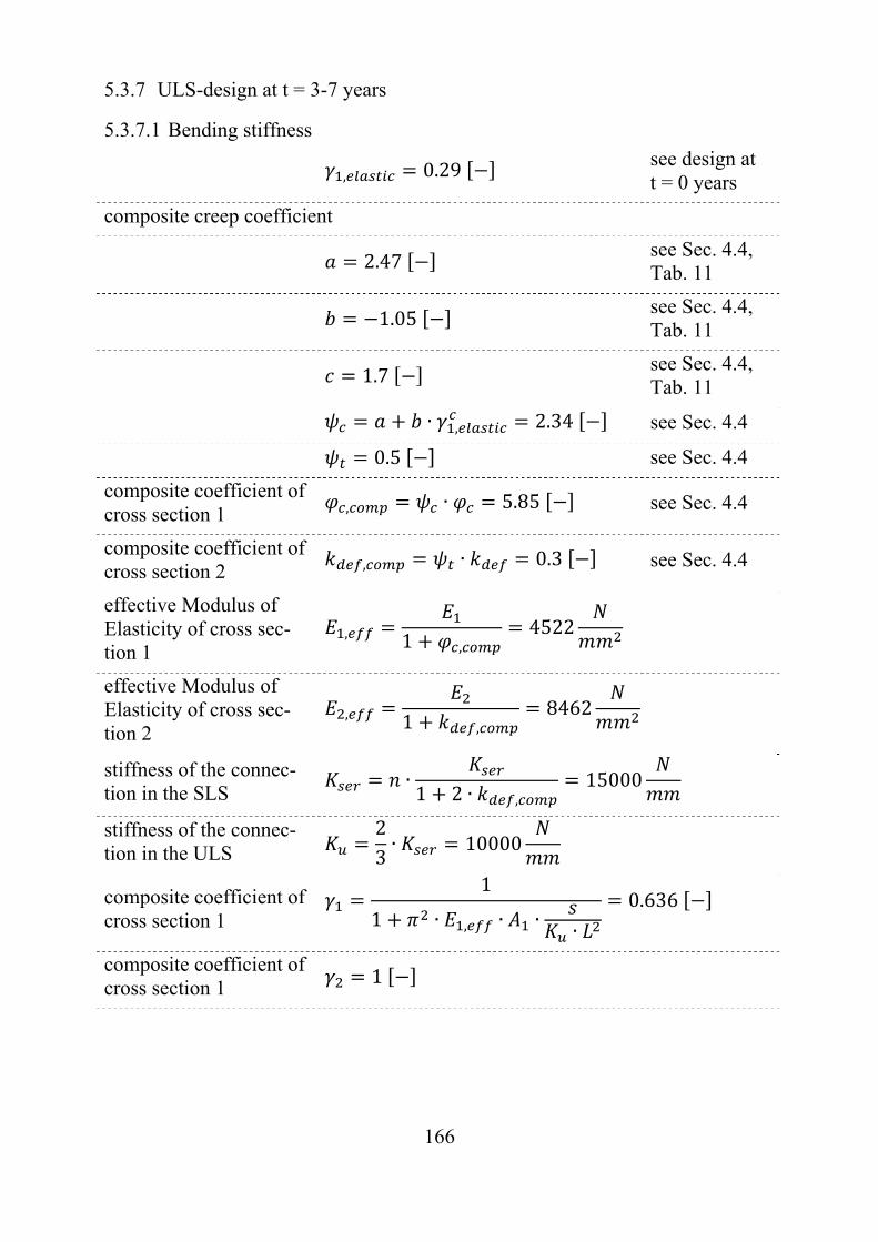
166
5.3.7 ULS-design at t = 3-7 years
5.3.7.1 Bending stiffness
, 0.29 see design at t = 0 years
composite creep coefficient
2.47 see Sec. 4.4, Tab. 11
1.05 see Sec. 4.4, Tab. 11
1.7 see Sec. 4.4, Tab. 11
∙ , 2.34 see Sec. 4.4
0.5 see Sec. 4.4
composite coefficient of cross section 1 , ∙ 5.85 see Sec. 4.4
composite coefficient of cross section 2 , ∙ 0.3 see Sec. 4.4
effective Modulus of Elasticity of cross sec-tion 1
, 1 ,4522
effective Modulus of Elasticity of cross sec-tion 2
, 1 ,8462
stiffness of the connec-tion in the SLS
∙1 2 ∙ ,
15000
stiffness of the connec-tion in the ULS
23∙ 10000
composite coefficient of cross section 1
1
1 ∙ , ∙ ∙ ∙
0.636
composite coefficient of cross section 1
1
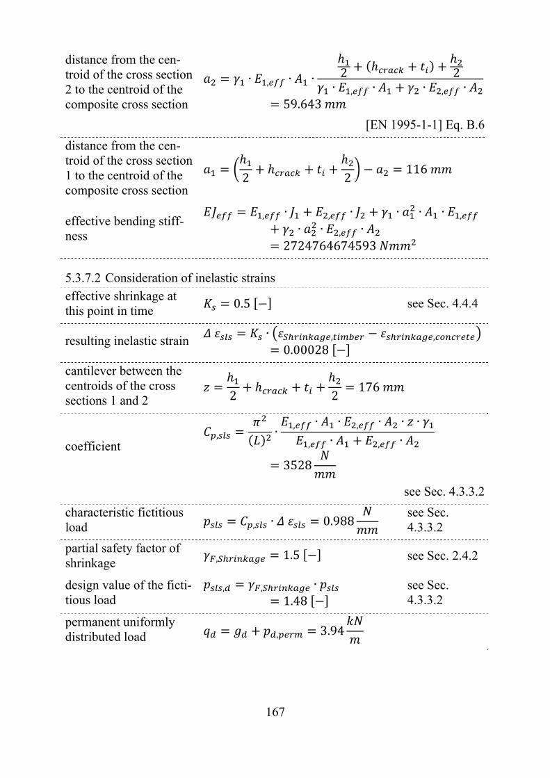
167
distance from the cen-troid of the cross section 2 to the centroid of the composite cross section
∙ , ∙ ∙ 2 2∙ , ∙ ∙ , ∙
59.643
[EN 1995-1-1] Eq. B.6
distance from the cen-troid of the cross section 1 to the centroid of the composite cross section
2 2116
effective bending stiff-ness
, ∙ , ∙ ∙ ∙ ∙ ,
∙ ∙ , ∙2724764674593
5.3.7.2 Consideration of inelastic strains
effective shrinkage at this point in time
0.5 see Sec. 4.4.4
resulting inelastic strain ∙ , ,
0.00028
cantilever between the centroids of the cross sections 1 and 2 2 2
176
coefficient , ∙ , ∙ ∙ , ∙ ∙ ∙
, ∙ , ∙
3528
see Sec. 4.3.3.2
characteristic fictitious load , ∙ 0.988
see Sec. 4.3.3.2
partial safety factor of shrinkage , 1.5 see Sec. 2.4.2
design value of the ficti-tious load
, , ∙1.48
see Sec. 4.3.3.2
permanent uniformly distributed load , 3.94
168
modification coefficient of the bending stiffness
,,
, ∙ , ∙∙ , ∙ , ∙ ∙
1.06
see Sec. 4.3.3.2
effective bending stiff-ness with respect to the inelastic strains
, , ∙2885840431672
see Sec. 4.3.3.2
5.3.7.3 Forces
5.3.7.3.1 External forces
coefficient 0.8
see Sec. 4.3.3.2 and [Schänzlin, 2003]
permanent bending moment without the fic-titious load
, , , , ∙8
12.778
bending moment caused by the fictitious load , , , ∙ , ∙
83.85
permanent bending moment
, , , , , , , ,
16.632
permanent shear force , , , ∙2
10.051
shear force caused by inelastic strain
∙ , ∙
∙ , ∙ , ∙
∙ , ∙ , ∙ ∙ ∙∙ 938
see Sec. 4.3.3.2, [Schänzlin, 2003] and [Schänzlin and Fragiacomo, 2007]
resulting permanent shear force , , , , 9.11
169
5.3.7.3.2 Internal forces of the single components
permanent bending moment in the concrete cross section
, , , ∙,
∙ , ,
0.146
permanent bending moment in the timber cross section
, , , ∙,
∙ , ,
4.33
permanent normal force in timber and concrete
,, , ,
, , , ,
47.319
5.3.7.4 Stresses in the concrete section and verification
5.3.7.4.1 Stresses
permanent stress caused by the normal force in the cross section
, ,, 1.421
permanent stress caused by the bending moment in the cross section
, ,, , 0.586
short term stress caused by the normal force in the cross section
, , 0.946 see design at t = 0 years
short term stress caused by the bending moment in the cross section
, , 0.936 see design at t = 0 years
resulting stress caused by the normal force in the cross section
, , , , , 2.367
resulting stress caused by the bending moment in the cross section
, , , , , 1.52
minimum stress , , , 3.89
maximum stress , , , 0.845
170
5.3.7.4.2 Verification of the stresses in the concrete
design strength in com-pression ∙ , 14.167
design strength in ten-sion ∙ , , , , 1.02
[EN 1992-1-1] Eq. 3.16
, 0.275
, 0.828
5.3.7.5 Stresses in the timber cross section and verification
5.3.7.5.1 Normal stresses
5.3.7.5.1.1 Stresses in the timber cross section and verification
permanent stress caused by the normal force in the cross section
, ,, 2.15
permanent stress caused by the bending moment in the cross section
, ,, , 5.36
short term stress caused by the normal force in the cross section
, , 1.43 see design at t = 0 years
short term stress caused by the bending moment in the cross section
, , 1.62 see design at t = 0 years
resulting stress caused by the normal force in the cross section
, , , , , 3.58
resulting stress caused by the bending moment in the cross section
, , , , , 6.99
171
5.3.7.5.1.2 Verification of the normal stresses
design strength in ten-sion , , ∙ , , 8.62
design strength in bend-ing , ∙ , 14.769
,
, ,
,
,0.889
5.3.7.5.2 Shear stresses
5.3.7.5.2.1 Determination of the shear stresses
distance from the lower edge to the centroid of the composite cross sec-tion
2170
permanent shear stress , 0.5 ∙ ∙ ,
,∙ , ,
0.583
[EN 1995-1-1] B.9
short term shear stress , 0.37 [EN 1995-1-1] B.9
resulting shear stress , , , 0.953
5.3.7.5.2.2 Verification of the shear
design strength in shear , ∙ , 2.46
,
,0.387
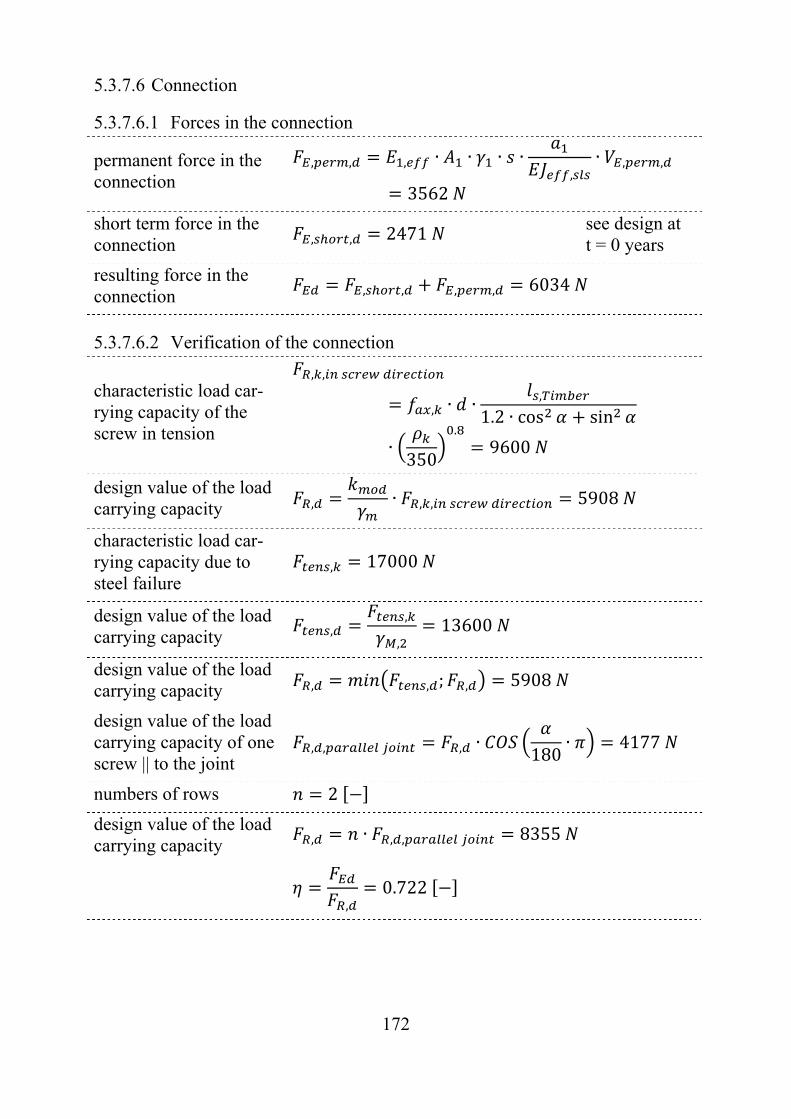
172
5.3.7.6 Connection
5.3.7.6.1 Forces in the connection
permanent force in the connection
, , , ∙ ∙ ∙ ∙,
∙ , ,
3562
short term force in the connection , , 2471 see design at
t = 0 years
resulting force in the connection , , , , 6034
5.3.7.6.2 Verification of the connection
characteristic load car-rying capacity of the screw in tension
, ,
, ∙ ∙ ,
1.2 ∙ cos sin
∙350
.9600
design value of the load carrying capacity , ∙ , , 5908
characteristic load car-rying capacity due to steel failure
, 17000
design value of the load carrying capacity ,
,
,13600
design value of the load carrying capacity , , ; , 5908
design value of the load carrying capacity of one screw || to the joint
, , , ∙180
∙ 4177
numbers of rows 2
design value of the load carrying capacity , ∙ , , 8355
,
0.722
173
5.3.8 SLS-design at t = 3-7 years
Since the creep deformations of the concrete, of the timber as well as of the con-nection have not yet reached their final values, the deformation at the time peri-od of 3 to 7 years is lower than the deformation at the point in time of 50 years. Therefore the serviceability limit state does not be checked for the time period between 3 and 7 years.

174
175
6. Summary, conclusions and outlook
6.1 Summary and conclusion
Timber-concrete-composite systems combine the advantages of pure timber decks with the advantages of pure concrete decks. In order to benefit from these advantages, the composite structure has to be designed. This design process is influenced by various parameters such as
Influences due to changing environmental conditions such as temperature and/or relative humidity
Influence of the erection process Behaviour of the connections between timber and concrete Non-linearity of the concrete Long term behaviour of the components
In this report the current state of the art regarding these issues is summarized.
The first step in a design process is to determine the loads, to choose the material and to estimate a first dimension of the cross section. For the design of timber concrete composite structures this step is quite similar to the design of pure tim-ber or pure concrete slabs. The major difference is that the effect of inelastic strains caused by temperature variation, shrinkage of concrete and swell-ing/shrinkage of timber has to be considered in the ULS as well as in the SLS. Most of the values are already given in the [EN1990] series. However the partial safety factor for the consideration of shrinkage is not given. A first attempt for this value is shown in this report.
The next important step in the design is to choose an appropriate connection be-tween timber and concrete. One major focus of the recent research and devel-opment was the determination of the properties of these connections. Therefore various connection devices exist. Some of them have a technical approval. The range of application of these connections depends on the type of load transfer, so it is up to the designer to choose the best connections. The summary of the most often used connection devices and a summary of the systems with a technical approval are given in the Sec. 0 of this report.
The connections between timber and concrete (except glued connections) are flexible connections, so forces in the connections will lead to deformations. These deformations in the joint between timber and concrete reduce the effec-tiveness of the composite action. In order to consider these deformations various methods for the evaluation of the internal forces have been proposed (see Sec. 0 and Annex B). Some of these methods have been derived in order to model tim-ber-timber-composite beams. So these methods can be used if the properties of concrete are considered in the evaluation of the forces. One influencing property
176
of concrete is that it cracks in tension. So during the evaluation of the force only the effective concrete cross section dimensions can be considered. Another im-portant parameter is the long term behaviour of both materials and the connec-tions. Since a composite beam is a hyper static system, the long term behaviour (as creep of the components timber, concrete and connection and inelastic strains) leads to a stress-redistribution within the composite cross section. This stress-redistribution itself influences the creep deformation. Besides, the creep strain of timber does not develop affine to the creep strain of concrete, leading to critical points in time. Therefore in Sec. 0 the determination of the internal forc-es in the short as well as in the long term is introduced with respect to the most important influences as creep, shrinkage and flexibility of the connections, con-cluded with an example of the design for quasi permanent climate.
6.2 Outlook
Despite this state-of-the-art-report there are several open questions when design-ing and realizing timber-concrete-composite structures. Some of these open questions are:
Reliability and partial safety factors: the internal forces are strongly influ-enced by the stiffness of the components. At the moment it is assumed, that the mean values are precise enough for the evaluation of the internal forces. The question remains, whether there should be an upper and a lower limit of the stiffness in order to determine the decisive internal forc-es?
Continuous beams: Most of the research has been focused on single span systems. However the question is, whether these results can be transferred to continuous systems?
Cracking of concrete: Concrete in tension cracks. In certain circumstances the connection device is anchored in the cracked area. Is there any influ-ence of the cracks on the properties of the connection?
Material: Most of the research has been done with "normal" materials. However it is expected, that a new combination of materials or use of ma-terials with a higher performance will lead to new open questions, which cannot be covered be the current state-of-the-art.
Dimensions: The research and development focusses on buildings. In buildings the slab sizes are smaller compared to bridges. Is there any in-fluence on the dimensions?
So the list of open questions could be continued, showing that there is knowledge about the design and the realization of timber-concrete-composite structures, but there are still open questions. So the times ahead will be very in-novative and interesting on the field of timber-concrete-composite structures.
177
7. References
7.1 References
[AASHO, 1949] AASHO 1949. 5th Standard Specifications for Highway Bridges. Washington, D.C.: The American Association of Highway Officials.
[AASHTO, 1983] AASHTO 1983. Standard Specifications for Highway Bridges 1983. Washington, D.C.: The American Asso-ciation of Highway Officials.
[Aicher, 1987] Aicher, S.: Bemessung biegebeanspruchter Sandwich-balken mit dem modifizierten γ-Verfahren. In: Bautech-nik (1987), No. 3, pp. 79–86, 1987
[Auclair et al., 2016] Auclair, S.; Sorelli, L.; Salenikovich, A.: Simplified nonlinear model for timber-concrete composite beams. International Journal of Mechanical Sciences 117: 30-42, 2016.
[Baldock and McCullough, 1941]
Baldcock, R.H.; McCullough, C.B: Loading test on a new composite type short span highway bridge combin-ing concrete and timber in flexure / Oregon State High-way Department. 1941 (Technical Bulletin No.1. Salem (USA)), 1941.
[Bejtka and Blaß, 2002]
Bejtka, I.; Blaß, H. J.: Joints with inclined screws. CIB-W18/35-7-4, Kyoto, Japan, 2002.
[Blaß et al., 1995] Blaß, H.-J.; Ehlbeck, J.; Linden, M. v. d.; Schlager, M.: Trag- und Verformungsverhalten von Holz-Beton-Verbundkonstruktionen. 1995 ( T2710)
[Blaß et al., 1996] Blaß, H.-J.; Ehlbeck, J.; Linden, M. L. R.; Schlager, M.: Trag- und Verformungsverhalten von Holz-Beton-Verbundkonstruktionen. bauen mit holz (1996), 5, pp. 392 – 399
[Bou Saïd, 2003] Bou Saìd, E.: Contribution à la modelisation des effets différes du bois et du béton sous conditions climatiques variables. Application aux structures mixtes bois-béton, PhD-thesis, Lyonm 2003
178
[Brunner and Schnüriger, 2006]
Brunner, M.; Schnüriger, M.: Adhesive connection for timber-concrete-composite. 9th World Conference on Timber Engineering, WCTE 2006, Portland, USA pp. 171, 2006
[Brunner et al., 2007] Brunner, M.; Romer, M.; Schnüriger, M.: Timber-concrete-composite with an adhesive connector (wet on wet process). Materials and Structures, 40, 119-126, 2007.
[Bursi et al., 2003] Bursi, O.S.; Ballerini, M.; Piazza, M.; Zandonini, R.; Fournely, E.; Kuhlmann, U.; Kürschner, K.;Schänzlin, J.: Shear transfer in composite members: testing, model-ling, standards and damage. COST C12, 2003 (Interna-tional Seminar, Lisbon, 19-20 April 2002), p. 21–36
[Calado et al., 2009] Calado L.; Proenca J.; R., G. 2009. ProHiTech WP7 Da-ta Sheets. Naples.
[Calil, 2006] Calil, J. C. 2006. Handbook for the Design and Con-struction of Timber Bridges. 9th World Conference on Timber Engineering, WCTE 2006, Portland, USA, 2006.
[Capretti et al., 1998] Capretti, S.; Ceccotti, A.; del Senno, M.; Lauriola, M.: On the Experimental Determination of Strength and De-formation Characteristics of Timber-Concrete Compo-site Joints. 5th World Conference on Timber Engineer-ing, WCTE 1998, Montreux, Switzerland, 1998.
[Ceccotti, 1995] Ceccotti, A.: STEP lecture E13: Timber-concrete com-posite structures. Timber Engineering – STEP 2. The Netherlands, 1995
[Ceccotti, 2002] Ceccotti, A.: Composite concrete-timber structures. Progress in Structural Engineering Materials, 4, 264-275, 2002.
[Crews and Gerber, 2010]
Crews, K.; Gerber, C.: Development of design proce-dures for timber concrete composite floors in Australia and New Zealand. CIB-W18/43-7-5, Nelson - New Zea-land, 2010.
[CSA, 2006] CSA. Canadian Highway Bridge design Code. Ontario, Canada: Canadian Standards Association 2006.
[Dabaon et al., 1993] Daboan, M.; Tschemmernegg, F.; Hassen, K.; Lateef, T. A.: Zur Tragfähigkeit von Verbundträgern bei teil-weiser Verdübelung. Stahlbau 62 (1993), pp. 3–9
179
[Dias and Jorge, 2011]
Dias, A. M. P. G.; Jorge, L. F. C.: The effect of ductile connectors on the behaviour of timber-concrete compo-site beams. Engineering Structures, 33, 3033-3042, 2011.
[Dias et al., 2004] Dias, A. M. P. G.; van de Kuilen, J. W. G.; Cruz, H. M. P.; Lopes, S. M. R.; Influence of interlayer on the be-haviour of timber-concrete composites. International Symposium on advanced timber and timber-composite elements for buildings - Design, construction, manufac-turing and fire safety. Florence, Italy: COST E29, 2004.
[Dias et al., 2007] Dias, A. M. P. G.; Lopes, S. M. R.; van de Kuilen, J. W. G.; Cruz, H. M. P.: Load-carrying capacity of timber-concrete joints with Dowel-type fasteners. Journal of Structural Engineering, ASCE, 133, 720-727, 2007.
[Dias et al., 2010] Dias, A. M. P. G.; Cruz, H. M. P.; Lopes, S. M. R.; van de Kuilen, J. W.: Stiffness of dowel-type fasteners in timber-concrete joints. Proceedings of the Institution of Civil Engineers-Structures and Buildings, 163, 257-266, 2010.
[Dias et al., 2015] Dias, A. M. P. G.; Martins, A. R. D.; Simones, L. M. C.; Providencia, P. M.; Andrade, A. A. M.: Statistical anal-ysis of timber-concrete connections - Mechanical prop-erties. Computers & Structures, 155, 67-84, 2015.
[Dias et al., 2018] Dias, A. M. P. G.; Fragiacomo, M.; Harris, R.; Kuklic, P.; Rajicic, V.; Schänzlin, J.: Technical Specification – Final Draft - Eurocode 5: Design of Timber Structures - Part 1-3: Structural design of timber concrete composite structures – Final Draft / Project Team CEN/TC 250-SC5.T2. 2018.
[Dias et al., 2018a] Dias, A. M. P. G.; Fragiacomo, M.; Harris, R.; Kuklic, P.; Rajicic, V.; Schänzlin, J.: Technical Specification – Background Document; Eurocode 5: Design of Timber Structure; Structural design of timber-concrete compo-site structures – common rules and rules for buildings / Project Team CEN/TC 250-SC5.T2. 2018.
[Dias, 1999] Dias, A. M. P. G. 1999. Estruturas mistas madeira-betão. Msc.
[Dias, 2005] Dias, A. M. P. G. 2005. Mechanical behaviour of tim-ber-concrete joints. PhD, Delft University of Technolo-gy.
180
[Dias, 2012] Dias, A. M. P. G. 2012. Analysis of the Nonlinear Be-havior of Timber-Concrete Connections. Journal of Structural Engineering, ASCE, 138, 1128-1137.
[Dias, 2016] Dias, A. 2016. Timber-concrete composites – a new part in Eurocode 5. 14th World Conference on Timber Engi-neering, WCTE 2016, Vienna, Austria, 2016.
[DIN 1052:1988] DIN 1052: Structural use of timber; design and con-struction, DIN-Deutsches Institut für Normung e.V., 1988
[DIN EN 1992-1-1, NA]
National German Annex to DIN EN 1992-1-1: Euro-code 2: Bemessung und Konstruktion von Stahlbeton- und Spannbetontragwerken - Teil 1-1: Allgemeine Be-messungsregeln und Regeln für den Hochbau; Deutsche Fassung EN 1992-1-1:2004 + AC:2010. DIN-Deutsches Institut für Normung e.V., 2010
[Dischinger, 1939] Dischinger, F.: Elastische und plastische Verformungen der Eisenbetontragwerke und insbesondere der Bogen-brücke. Der Bauingenieur 14 (1939), No. 5 and 6, pp. 53–63
[Döhrer and Raut-enstrauch, 2006]
Döhrer, A.; Rautenstrauch, K.: Connectors for timber-concrete-composite-bridges. CIB-W18/39-7-3, 2006
[Ehlbeck and Larsen, 1993]
Ehlbeck, J.; Larsen, H. J. 1993. Eurocode 5 – Design of timber structures: Joints. Society, F. P. (ed.) Proceed-ings, International workshop on wood connectors. Mad-ison, USA.
[Ehlbeck et al., 1967] Ehlbeck, J.; Köster, P.; Schelling, W.: Praktische Berechnung und Bemessung nachgiebig zusammeng-esetzer Holzbauteile. bauen mit Holz (1967), pp. 289 – 294
[EN 13501-1] EN 13501-1: Fire classification of construction products and building elements - Part 1: Classification using data from reaction to fire tests; German and English version prEN 13501-1:2017
[EN 14080] EN 14080 Timber structures - Strength graded structural timber with rectangular cross section - Part 1: General requirements; German version EN 14081-1:2016
181
[EN 1990] Eurocode: Basis of structural design; German version EN 1990:2002 + A1:2005 + A1:2005/AC:2010
[EN 1991-1-1] EN 1991-1-1 Eurocode 1: Actions on structures - Part 1-1: General actions - Densities, self-weight, imposed loads for buildings;
[EN 1991-1-5] EN 1991-1-5 Eurocode 1: Actions on structures - Part 1-5: General actions - Thermal actions;
[EN 1992-1-1] EN 1992-1-1 Eurocode 2: Design of concrete structures – Part 1-1: General rules and rules for buildings; EN 1992-1-1:2004 + AC:2010
[EN 1994-1-1] EN 1994-1-1 Eurocode 4 - Design of composite steel and concrete structures - Part 1-1: General rules and rules for buildings. Brussels: CEN 2004.
[EN 1995-1-1] EN 1995-1-1 Eurocode 5 - Design of timber structures - Part 1-1: General - Common rules and rules for build-ings. Brussels: CEN 2004.
[EN 1995-2] EN 1995-2 Eurocode 5 - Design of timber structures - Part 2: Bridges. Brussels: CEN 2004.
[EN 206-1] EN 206-1: Concrete - Part 1: Specification, perfor-mance, production and conformity; German version EN 206-1:2017
[EN 26891] EN 26891 - Timber structures - Joints made with me-chanical fasteners - General principles for the determi-nation of strength and deformation characteristics. ISO EN 26891.
[EN 338] EN 338 Structural timber – Strength classes
[ETA 12-0196] ETA 12-0196: Timtec plus VG screw Self-tapping screws for use in wood-concrete slab kits; SWG Schraubenwerk Gaisbach GmbH, Am Bahnhof 50, DE-74638 Waldenburg.
[ETA-13/0029] ETA-13/0029: Self-tapping screws for use in wood-concrete slab, Adolf Würth GmbH & Co. KG.
[Eyberg, 1981] Eyberg, T.: Geschlossene Darstellung der Spannung-sumlagerung in Verbundkonstruktionen. Beton- und Stahlbeton H 12, pp. 301–304, 1981
182
[Foschi, 1974] Foschi, R. O.: Load-slip Characteristics of Nails. Wood Science, 7, 69-76, 1974.
[Fragiacomo and Schänzlin, 2010]
Fragiacomo, M.; Schänzlin, J.: The Effect Of Moisture And Temperature Variations On Timber-Concrete Composite Beams. 11th World Conference on Timber Engineering 2010, WCTE 2010, Myasaki, Japan, pp. 113–120, 2010
[Fragiacomo and Schänzlin, 2013]
Fragiacomo, M.; Schänzlin, J.: Proposal to account for environmental effects in design of timber-concrete composite beams, Journal of Structural Engineering, ASCE, Vol 39, No. 1 pp. 162-167, 2013
[Fragiacomo, 2000] Fragiacomo, M.: Comportamento a lungo termine di travi composte legno-calcestruzzo, University of Tri-este, PhD-thesis, 2000
[Frangi, 2001] Frangi, A.: Brandverhalten von Holz-Beton-Verbunddecken. ETH Zürich, 2001
[Fries, 2001] Fries, J.: Tragverhalten von Flachdecken mit Hutpro-filen, PhD-Thesis, Institut für Konstruktion und Entwurf, University of Stuttgart, 2001, http://elib.uni-stuttgart.de/opus/volltexte/2002/985/
[Gelfi et al., 2002] Gelfi, P., Giuriani, E.; Marini, A.: Stud shear connection design for composite concrete slab and wood beams. Journal of Structural Engineering, ASCE, No. 128, pp. 1544-1550, 2002
[Gerber et al., 2012] Gerber, C., Crews, K.; Shrestha, R.; Design Guide Aus-tralia and New Zealand - Timber Concrete Composite Floor Systems. Company, S. T. I. (ed.). Christchurch: Structural Timber Innovation Company, 2012.
[Gramatikov, 2008] Gramatikov, K.: ProHiTech WP7 Final Report. Civil Engineering faculty, Skopje, 2008.
[Grosse and Raut-enstrauch, 2004]
Grosse, M.; Rautenstrauch, K.: Numerical modelling of timber and connection elements used in timber-concrete-composite constructions CIB-W18/37-7-15, Edinburgh, 2004.
183
[Grosse et al., 2003] Grosse, M.; Hartnack, R.; Lehmann, S.; Rautenstrauch, K.: Modellierung von diskontinuierlich verbundenen Holz-Beton-Verbundkonstruktionen. Bautechnik 80 (2003), pp. 534 – 541 and 693 – 701, 2003
[Hamm and Richter, 2009]
Hamm, P.; Richter, A.: Bemessungs- und Kon-struktionsregeln zum Schwingungsnachweis von Holzdecken. Fachtagungen Holzbau 2009 Landesbeirat Holz Baden-Württemberg e.V., Stuttgart, 2009, pp. 15 – 29. – Leinfelden-Echterdingen, 26. November 2009
[Hamm, 2004] Hamm, P.: Schwingungen von Wohnungsdecken und Fußgängerbrücken. Holz ... im Zusammenspiel mit an-deren Baustoffen – Fachtagungen Holzbau 2004, Infor-mationsdienst Holz, pp. 152–160, 2004.
[Holschemacher et al., 2013]
Holschemacher, K.; Selle, R.; Schmidt, J.; Kieslich, H.: Holz-Beton-Verbund – Betonkalender 2013 pp. 241-287, 2013
[Hösslin and Ladner, 1996]
Hösslin, T. V.; Ladner, M.: Untersuchungsbericht 1235-2: Prüfung des Haftverbundes zwischen Holz und Beton unter dynamischer Belastung, 1996.
[Hösslin and Ladner, 1996a]
Hösslin, T. V.; Ladner M.: Untersuchungsbericht 1235-1: Prüfung des Haftverbundes zwischen Holz und Beton unter statischer Belastung, 1996.
[Hösslin and Ladner, 1996b]
Hösslin, T. V.; Ladner M.: Untersuchungsbericht 1235-3: Prüfung des Haftverbundes zwischen Holz und Beton unter statischer Belastung 1996.
[Hösslin and Ladner, 1996c]
Hösslin, T. V.; Ladner M.: Untersuchungsbericht 1235-4: Prüfung des Haftverbundes zwischen Holz und Beton unter statischer Belastung, 1996.
[Hösslin and Ladner, 1998]
Hösslin, T. V.; Ladner, M.: Untersuchungsbericht 1235-5: Prüfung des Haftverbundes zwischen Holz und Beton unter statischer Belastung 1998.
[JCSS, 2001] Probabilistic model code, Joint Committee on Structural Safety, 2001
184
[Jorge et al., 2010] Jorge, L.; Schänzlin, J.; Lopes, S.; Cruz, H.; Kuhlmann, U.: Time-dependent behaviour of timber lightweight concrete composite floors. Engineering Structures, ASCE 32 (2010), 12, S. 3966 – 3973, 2010
[Jorge, 2005] Jorge, L. F. d. C.: Estruturas mistas madeira-betão com a utilização de betões de agregados leves/Timber-concrete structures using lightweight aggregate con-crete. (PhD), University of Coimbra, 2005.
[Jung, 2000] Jung, P.: Der gedübelte Brettstapel. 6. Internationales Holzbau Forum. 2000.
[Junior et al., 2006] Junior, C. C., Dias, A. A., Goés, J. L. N., Cheung, A. B., Stamano, G. C., Pigozzo, J. C., Okimoto, F. S., Logsdon, N. B., Brazolini, S.; Lana, E. L.: Manual de Projeto e Construção de Pontes de Madeira, São Carlos, Brasil, SET-EESC – USP, 2006.
[Kenel and Meierho-fer, 1998]
Kenel, A.; Meierhofer, U.: Holz / Beton-Verbund unter langfristiger Beanspruchung. EMPA Dübendorf (CH), Abteilung Holz, 1998 (Research report 115/39)
[Kenel, 2000] Kenel, A.: Zur Berechnung von Holz/Beton-Verbundkonstruktionen. EMPA Dübendorf (CH), Ab-teilung Holz, 2000 (Report 115/42)
[Kerler, 2016] Kerler, V.: Erste Auswertungen zum Teilsicherheits-beiwert des Schwindens, Masterthesis HTWG Kon-stanz, 2016
[Kevarinmaki, 2002] Kevarinmaki, A. Joints with inclined screws. CIB-W18/35-7-3, Kyoto, Japan, 2002.
[Khorsandnia et al., 2014]
Khorsandnia, N.; Schänzlin, J.; Valipour, H.; Crews, K.: Time-dependent behaviour of timber-concrete compo-site members: Numerical verification, sensitivity and influence of material properties. Construction and Building Materials 66, pp. 192–208, 2014. http://dx.doi.org/http://dx.doi.org/10.1016/j.conbuildmat.2014.05.079. – DOI http://dx.doi.org/10.1016/j.conbuildmat.2014.05.079
185
[Khorsandnia et al., 2015]
Khorsandnia, N.; Schänzlin, J.; Valipour, H.; Crews, K.: Coupled finite element-finite difference formulation for long-term analysis of timber-concrete composite struc-tures. Engineering Structures 96, pp. 139 – 152, 2015
[Kostica et al., 2018] Kostica, S; Merka, V.; Berba, J.; Hassa, P.; Burgerta, I.; Cabanea, E.: Timber-mortar composites: The effect of sol-gel surface modification on the wood-adhesive inter-face. Composite Structures, No. 201, pp. 828-832, 2018.
[Kreuzinger, 1994] Kreuzinger, H.: Verbundkonstruktionen Holz / Beton. 1994
[Kreuzinger, 1999a] Kreuzinger, H.: Holz-Beton-Verbundbauweise. Fachtagungen Holzbau 1999-2000: Holzbau für das neue Jahrhundert, Informationsdienst Holz, pp. 70 – 83, 1999
[Kreuzinger, 1999b] Kreuzinger, H.: Flächentragwerke: Platten, Scheiben und Schalen; Berechnungsmethoden und Beispiele. In-formationsdienst Holz: Brücken aus Holz; pp. 43-60; 1999
[Kudla, 2015] Kudla, K.: Short Term Scientific Mission: Notched Connections for TCC Structures as Part of the Standard. Cost Action FP1402, 2015
[Kuhlmann and Rieg, 2004]
Kuhlmann, U.; Rieg, A.: Mittragende Betongurtbreite niedriger Verbundträger / Institut für Konstruktion und Entwurf, University of Stuttgart.– AiF-research report No. 13460 N/1, 2004.
[Kuhlmann and Schänzlin, 2008]
Kuhlmann, U.; Schänzlin, J.: A timber-concrete compo-site slab system for use in tall buildings. Structural En-gineering International 18, No. 2, pp. 174–178, 2008
[Kuhlmann et al., 2001]
Kuhlmann, U.; Fries, J.; Rieg, A.: Composite Girders with Reduced Height. Connections between Steel and Concrete RILEM, Proceedings PRO 21, RILEM Publi-cations S.A.R.L., S. 1371–1381, 2001.
186
[Kuhlmann et al., 2006]
Kuhlamm, U.; Schänzlin, J.; Merkle, R.; Bux, H.: Brettstapel-Beton-Verbunddecken mit integrierten Slim-Floor-Profilen / Institut für Konstruktion und Entwurf, University of Stuttgart. – Research report funded by Deutsche Bundesstiftung Umwelt AZ 21168, 2006.
[Kupfer and Kirmair, 1987]
Kupfer, H.; Kirmair, H.: Verformungsmoduln zur Berechnung statisch unbestimmter Systeme aus zwei Komponenten mit unterschiedlichen Kriechzahlen. Bauingenieur 62, pp. 371–377, 1987
[Kupfer, 1958] Kupfer, H.: Kräfteumlagerung durch Kriechen bei un-terschiedlichen Kriechzahl der verwendeten Baustoffe. Monographie der DYWIDAG, 1958
[Lehmann, 2004] Lehmann, S.: Untersuchungen zur Bewertung von Ver-bundbauteilen aus Brettstapelelementen im Flächen-verbund mit mineralischen Deckschichten. Bauhaus-Universität Weimar, 2004.
[Magalhães, 1997] Magalhães, L.: Vigas compostas madeira/concreto. MsC, Universidade Federal de Minas Gerais, 1997.
[McCullough, 1934] McCullough, C. B.: Highway Viaducts in Oregon of Prefabricated Timber. Wood Preserving News, XII, 1934.
[McCullough, 1943] McCullough, C. B.: Oregon Tests on Composite (Tim-ber-Concrete) Beams. Journal of the American Concrete Institute, No. 14, pp. 429-440, 1943.
[Michelfelder, 2006] Michelfelder, B.: Trag- und Verformungsverhalten von Kerven bei Brettstapel-Beton-Verbunddecken, Universi-ty of Suttgart, Institut für Konstruktion und Entwurf, PhD-thesis, 2006. http://nbn-resolving.de/urn:nbn:de:bsz:93-opus-28911
[Möhler, 1956] Möhler, K.: Über das Tragverhalten von Biegeträgern und Druckstäben mit zusammengesetztem Querschnitt und nachgiebigen Verbindungsmitteln, habilitation, Karlsruhe 1956.
187
[Monteiro et al., 2010]
Monteiro, S. R. S.; Dias, A. M. P. G.; Negrao, J. H. J. O.: Experimental and Numerical Evaluation of Notched timber-concrete joints mechanical behaviour. 11th World Conference on Timber Engineering, WCTE 2010. Riva del Garda – Italy, 2010.
[Monteiro et al., 2013]
Monteira, S. R. S.; Dias, A. M. P. G.; Negrao, J. H. J. O.: Assessment of Timber-Concrete Connections Made with Glued Notches: Test Set-Up and Numerical Model-ing. Experimental Techniques, No. 37, pp. 50-65, 2013.
[Negrao et al., 2010a] Negrao, J. H. J. D.; de Oliveira, C. A. L.; de Oliveira, F. M. M.; Cachim, P. B.: Glued Composite Timber-Concrete Beams. I: Interlayer Connection Specimen Tests. Journal of Structural Engineering - ASCE, No. 136, pp. 1236-1245, 2010.
[Negrao et al., 2010b] Negrao, J. H. J. D.; de Oliveira, F. M. M.; de Oliveria, C. A. L.; Cachim, P. B.: Glued Composite Timber-Concrete Beams. II: Analysis and Tests of Beam Spec-imens. Journal of Structural Engineering - ASCE, No. 136, pp. 1246-1254, 2010.
[Nicolas, 2001] Nicolas, E. A.: Estudo de Ligações em Estruturas Mistas de Concreto-Madeira. Msc, Universidade Estadual de Campinas, 2001.
[Niederer, 2008] Niederer, A: Grenzen der Anwendung des -Verfahrens, HTWG Konstanz, Bachelor-thesis, 2008
[Ollgaard et al., 1971] Ollgaard, J. G., Slutter, R. G.; Fisher, J. W.: Shear Strength of Stud Connectors in Lightweight and Nor-mal-Weight Concrete. Engineering Journal - American Institute of Steel Construction Inc, No. 8, pp. 55, 1971.
[Postulka, 1998] Postulka, J.: Holz-Beton-Verbunddecken 36 Jahre Erfahrung. Bautechnik, No. 74, pp. 478- 480, 1997.
[Rautenstrauch, 2004]
Rautenstrauch, K.: Entwicklung der Holz-Beton-Verbundbauweise. König, G., Holschemacher, K., Dehn, F. (eds): Innovationen im Bauwesen, Holz-Beton-Verbund, S. 1-22. Bauwerk Verlag, Berlin, 2004.
188
[Richart and Wil-liams, 1943]
Richart, F. E.; Williams, C. B.: Tests of Composite Timber And Concrete Beams. University of Illinois Bul-letin 40, p. 62, 1943.
[Rieg, 2006] Rieg, A.: Verformungsbezogene mittragende Breite nie-driger Verbundträger, University of Suttgart, Institut für Konstruktion und Entwurf, PhD-thesis, 2006. http://nbn-resolving.de/urn:nbn:de:bsz:93-opus-29048
[RILEM-CT-111-CST, 1992]
RILEM-CT-111-CST. Behaviour of timber-concrete composite load-bearing structures. RILEM, ed. Proceed-ings of ACMAR-Ravenna International Symposium, 1992 Dept. of Civil Engineering, University of Flor-ence, Italy, 1992.
[Ruesch and Jungwirth, 1976]
Ruesch, H.; Jungwirth, D.: Stahlbeton, Spannbeton - Berücksichtigung der Einflüsse von Kriechen und Schwinden auf das Verhalten der Tragwerke. Werner-Verlag, 1976
[Schäfers and Seim, 2011]
Schäfers, M.; SEIM, W.: Investigation on bonding be-tween timber and ultra-high performance concrete (UHPC), Construction and Building Materials, No. 25, pp. 3078-3088, 2011.
[Schänzlin and Fragiacomo, 2007]
Schänzlin, J.; Fragiacomo, M.: Extension of EC5 Annex B formulas for the design of timber-concrete composite structures. CIB-W18/40-10-1, 2007
[Schänzlin, 2003] Schänzlin, J.: Zum Langzeitverhalten von Brettstapel-Beton-Verbunddecken, Institut für Konstruktion und Entwurf, University of Stuttgart, PhD-thesis, 2003
[Schänzlin, 2017] Schänzlin, J.: Is it necessary to consider moisture varia-tions in TCC? Report developed within the work of CEN/TC250/SC5/PT5.2, unpublished, 2017.
[Schmidt et al., 2003] Schmidt, J.; Schneider, W.; Thiele, R.: Zum Kriechen von Holz-Beton-Verbundkonstruktionen. Beton- und Stahlbetonbau 98 (2003), No. 7, pp. 399–407, 2003
189
[Schmidt et al., 2004] Schmidt, J.; Kaliske, M.; Schneider, W.; Thiele, R.: Bemessungsvorschlag für Holz-Beton-Verbundbalken unter Beachtung abgestufter Verbindungsmittel. Bautechnik 81 (2004), No. 3, pp. 172–179, 2004.
[Schober and Raut-enstrauch, 2006]
Schober, K. U.; Rautenstrauch, K.: Upgrading and re-pair of timber structures with polymer concrete facing and strengthening. 9th World Conference on Timber Engineering, WCTE 2006, Portland, USA, 2006.
[Schober et al., 2012] Schober, K.U.; Drass, M.: Advanced interface interac-tion in timber engineering joints with dowel-type fas-teners embedded in high-performance ceramic fillers. 12th World Conference on Timber Engineering, WCTE 2012, Auckland, New Zealand, 2012.
[Scholz, 2003] Scholz, A.: Ein Beitrag zur Berechnung von Flächen-tragwerken aus Holz, TU München, PhD-thesis., 2003
[Scholz, 2004] Scholz, A.: Eigenspannungszustände an Verbund-querschnitten infolge von Dehnungsunterschieden An-wendung eines neueren Rechenverfahrens auf einem bewährten Lösungsansatz. Bautechnik 81 (2004), No. 3, pp. 180–188, 2004
[Schönborn, 2006] Schönborn, F.: Holz-Beton-Fertigteilelemente. PhD, Leopold-Franzens-Universität, 2006.
[Seim et al., 2016] Seim, W.; Eisenhut, L.; Kühlborn, S.: Adhesive-Bonded Timber-Concrete Composites - Experimental Investiga-tion of Thermal-Hygric Effects. 14th World Conference on Timber Engineering, WCTE 2016, Vienna, Austria, 2016.
[Soriano, 2001] Soriano, J.: Estruturas Mistas em Concreto e em Madei-ra: Análise de Vigas e Painéis e Aplicações na Con-strução Civil. PhD, Universidade Estadual de Campinas, 2001.
[TiComTec, 2014] TiComTec: Load Bearing Constructions using Wood-Concrete-Composite Technique with glued-in HBV ® - Shear Connectors, 2014.
[Tononi and Usardi, 2010]
Tononi, D.; Usardi, I.: Moisture transfer and moisture induced stresses in timber structures under environmen-tal conditions in Europe. Cost E55 Report, 2010.
[Tschopp Holzbau AG, 2011]
Tschopp Holzbau AG: Bemessungstabellen. BRESTA, 2011.
190
[Van der Linden, 1999]
van der Linden, M.: Timber Concrete Composite Floors. PhD, Delft University of Technology, 1999.
[Winter et al., 2010] Winter, S.; Hamm, P.; Richter, A.: Schwingungs- und Dämpfungsverhalten von Holz- und Holz-Beton-Verbunddecken. Final report / TU München, Lehrstuhl für Holzbau und Baukonstruktion. Research report funded by the BMWA and the AiF, 2010.
[Yeoh et al., 2011] Yeoh, D.; Fragiacomo, M.; de Franceschi, M.; Boon, K. H.: State of the Art on Timber-Concrete Composite Structures: Literature Review. Journal of Structural En-gineering, pp. 1085-1095, 2011.
[Yeoh, 2010] Yeoh, D.: Behaviour and Design of Timber-Concrete Composite. PhD, University of Canterbury, 2010.
[Z-9.1-342] Z.-9.1-342: SFS VB Schrauben als Verbindungsmittel in Holz-Beton-Verbundkonstruktionen, SFS intec AG, Rosenbergsaustraßse 10, 9435 Heerbrugg, Schweiz.
[Z-9.1-445] Z.-9.1-445: Timco II und III Schrauben als Verbindungsmittel für das Timco Holz-Beton-Verbundsystem, Sieglinde Amrath – Timco II Vertrieb Deutschland, Kratellen 15, 78355 Hohenfels.
[Z-9.1-603] Z.-9.1-603: TCC Schrauben als Verbindungsmittel für das TCC Holz-Beton-Verbundsystem, Com-Ing AG, Alpsteinstrasse 15, 9050 Appenzell, Schweiz.
[Z-9.1-648] Z.-9.1-648: Würth ASSYplus VG Schrauben als Verbindungsmittel für Holz-Beton-Verbundkonstruktionen, Adolf Würth GmbH & Co.KG, Reinhold-Würth-Straße 12-17, 74653 Künzelsau-Gaisbach.
[Z-9.1-803] Z.-9.1-803: SWG Timtec VG Plus - Vollgewin-deschrauben als Verbindungsmittel für Holz-Beton-Verbundkonstruktionen, Schraubenwerk Gaisbach GmbH, Am Bahnhof 50, 74638 Waldenburg.
191
[Z-9.1-845] Z.-9.1-845: Star-Drive und RAPID Schrauben als Verbindungsmittel für das Schmid Schrauben Holz-Beton-Verbundsystem, Schmid Schrauben Hainfeld GmbH, Landstal 10, 3170 Hainfeld, Österreich.
[Z-9.1-851] Z.-9.1-851: BiFRi Verbund-Anker als Verbindungsmit-tel für das FRIEDRICH Holz-Beton-Verbundsystem, FRIEDRICH UG Verbundsysteme, Hofer Straßse 21, 95233 Helmbrechts.
[Z-9.1-857] Z.-9.1-857: SFix-3 Schubfix-Schraube als Verbindungsmittel für das Elascon Holz-Beton-Verbund-System (SFix-3 Elascon HBV-System), Elas-con GmbH, Am Rosengarten 4F, 79183 Waldkirch.
7.2 Additional references
[Ballerini et al., 2002] Ballerini, M.; Crocetti, R.; Piazza, M.: An experimental investigation on notched connections for timber-concrete composite structures. 7th World Conference on Timber Engineering, WCTE 2002, Shah Alam, Malay-sia, 2002.
[Bathon and Graf, 2000]
Bathon, L. H.; Graf, M.: A continuous wood-concrete-composite system. 6th World World Conference on Timber Engineering, WCTE 2000, British Columbia – Canada, 2000.
[Bathon and Clou-ston, 2004]
Bathon, L.; Clouston, P.: Experimental and numerical results on semi-prestressed wood-concrete composite floor systems for long-span applications. 8th World Conference on Timber Engineering, WCTE 2004, Lathi, Finland, 2004.
[Bathon et al., 2006] Bathon, L.; Bletz, O.; Bahmer, R.: Retrofit of Timber Bridges - A System Approach Using Prefabricated Wood-Concrete-Composite Element. 9th World Confer-ence on Timber Engineering, WCTE 2006, Portland, USA, 2006.
192
[Brunner et al. , 2007]
Brunner, M.; Romer, M.; Schnüriger, M.: Timber-concrete-composite with an adhesive connector (wet on wet process). Materials and Structures, No. 40(1), pp. 119-126, 2007.
[Carvalho and Car-rasco, 2010]
Carvalho, E. P.; Carrasco, E. V. M.: Influence of test specimen on experimental characterization of timber–concrete composite connections. Construction and Building Materials, No. 24(8), pp. 1313-1322, 2010.
[Ceccotti et al., 2006] Ceccotti, A.; Fragiacomo, M.; Giordano, S.: Behaviour of a Timber-Concrete Composite Beam with Glued Connection at Strength Limit State. 9th World Confer-ence on Timber Engineering, WCTE 2006, Portland, USA, 2006.
[Clouston et al., 2005]
Clouston, P.; Bathon, L. A.; Schreyer, A.: Shear and bending performance of a novel wood-concrete compo-site system. Journal of Structural Engineering - ASCE, No. 131(9), pp. 1404-1412, 2005.
[Clouston et al., 2004]
Clouston, P.; Civjan, S.; Bathon, L.: Experimental be-havior of a continuous metal connector for a wood-concrete composite system. Forest Products Journal, No. 54(6), pp. 76-84, 2004.
[Cloronado et al., 2006]
Coronado, M.; Triche, M.; Fridley, K.: Wood to Con-crete Connections. 9th World Conference on Timber Engineering, WCTE 2006, Portland, USA, 2006.
[Deam et al., 2006] Deam, B. L.; Fragiacomo, M.; Buchanan, A. H.: Con-nections for composite concrete slab and LVL flooring systems. Materials and Structures, No. 41(3), pp. 495-507, 2008.
[Dias, 1999] Dias, A. M. P. G.: Estruturas mistas madeira-betão. (Msc), Coimbra, 1999.
[Dias, 2005] Dias, A. M. P. G.: Mechanical behaviour of timber-concrete connections. (PhD), Delft University of Tech-nology, Delft, 2005.
193
[Dias et al., 2004] Dias, A. M. P. G.; Cruz, H. M. P.; Lopes, S. M. R.; Van de Kuilen, J. W. G.: Experimental shear-friction tests on dowel type fasteners timber-concrete connections. 8th Conference on Timber Engineering, WCTE 2004, Lathi, Finland, 2004.
[Döhrer and Raut-enstrauch, 2006]
Döhrer, A.; Rautenstrauch, K.: The Construction of Road Bridges as Timber-Concrete Composites. 9th World Conference on Timber Engineering, WCTE 2006, Portland, USA, 2006.
[Fast et al., 2003] Fast, R. S.; Gutkowski, R.; Criswell, M.; Radford, D.: Durability Studies of Layered Wood-Concrete Connec-tions and Beams. Retrieved from Colorado, USA, 2003.
[Faust and Selle, 1999]
Faust, T.; Selle, R.: Properties of Composite Connec-tions of Timber - LWAC Composite Structures. Re-trieved from University of Leipzig, Federal Republic of Germany, 1999.
[Fernandez-Cabo et al., 2012]
Fernandez-Cabo, J. L.; Arriaga, F.; Majano-Majano, A.; Iniguez-Gonzalez, G.: Short-term performance of the HSB (R) shear plate-type connector for timber-concrete composite beams. Construction and Building Materials, No. 30, pp. 455-462, 2012.
[Fragiacomo, 2012] Fragiacomo, M.: Experimental behaviour of a full-scale timber-concrete composite floor with mechanical con-nectors. Materials and Structures, No. 45(11), pp. 1717-1735, 2012.
[Fragiacomo and Yeoh, 2010]
Fragiacomo, M.; Yeoh, D.: Design of timber-concrete composite beams with notched connections. Paper pre-sented at the CIB-W18/43-7-4, Nelson, New Zealand, 2010.
[Fragiacomo et al., 2007]
Fragiacomo, M.; Amadio, C.; Macorini, L.: Short- and long-term performance of the "Tecnaria" stud connector for timber-concrete composite beams. Materials and Structures, No. 40(10), 2007.
[Girhammar, 1984] Girhammar, U. A.: Composite Timber and Concrete Components for Walls IABSE 1984, pp. 369-376, 1984.
194
[Gurkšnys et al., 2005]
Gurkšnys, K.; Kvedaras, A.; Kavaliauskas, S.: Behav-iour Evaluation of "Sleeved" Connectors in Composite Timber-Concrete Floors. Journal of Civil Engineering and Management, No. 11(4), pp. 277-282, 2005.
[Hemmy and Droese, 2000]
Hemmy, O.; Droese, S.: Verbunddecke aus Holzbalken und Elementdecken mit Stahlfaseraufbeton - Versuche mit Verbundmitteln. Bautechnik, No. 77(4), pp. 221-228, 2000.
[Holschemacher et al., 2004]
Holschemacher, K.; Klotz, S.; Köhler, S.: Ver-bunddecken aus Stahlfaserbeton und Holz. Beton- und Stahlbetonbau, No. 99(1), pp. 10-15, 2004.
[Inoue et al., 2002] Inoue, M.; Tanaka, K.; Yano, H.; Yoshioka, T.; Hayakawa, A.; Komatsu, K.; Kawai, N.: Development of Connecting System Between Reinforced Concrete and Timber. 7th World Conference on Timber Engi-neering, WCTE 2002, Shah Alam, Malasya, 2002.
[Jorge, 2005]
[Kanocz and Kuli-ková, 2006]
Kanocz, J.; Kuliková, D.: High performance timber-concrete composite slab systems with fiber reinforced concrete 9th World Conference on Timber Engineering, WCTE 2006, Portland, USA, 2006.
[Kanocz et al., 2013] Kanocz, J.; Bajzecerova, V.; Steller, S.: Timber-Concrete Composite Elements with Various Composite Connections Part 1: Screwed Connection. Wood Re-search, No. 58(4), pp. 555-569, 2013.
[Kanocz et al., 2014] Kanocz, J.; Bajzecerova, V.; Steller, S.: Timber -Concrete Composite Elements with Various Composite Connections Part 2: Grooved Connection. Wood Re-search, No. 59(4), pp. 627-638, 2014.
[Kavaliauskas et al., 2007]
Kavaliauskas, S.; Kvedaras, A.; Valiunas, B.: Mechani-cal behaviour of timber�to�concrete connections with inclined screws. Journal of Civil Engineering and Man-agement, No. 13(3), pp. 193-199, 2007.
195
[Khorsandnia et al., 2012]
Khorsandnia, N.: Valipour, H. R.; Crews, K.: Experi-mental and analytical investigation of short-term behav-iour of LVL-concrete composite connections and beams. Construction and Building Materials, No. 37, pp. 229-238, 2012.
[Kuhlmann and Aldi, 2008a]
Kuhlmann, U.; Aldi, P.: Fatigue of timber-concrete-composite beams: characterisation of the connection behaviour through push-out tests. 10th World Confer-ence on Timber Engineering, WCTE 2008, Miyazaki, Japan, 2008.
[Kuhlmann and Aldi, 2008b]
Kuhlmann, U.; Aldi, P.: Transferring shear forces in timber board stack-concrete composite floors without screws, research project DGfH/AiF 14497N (Nr. 2008-8X), 2008.
[Kuhlmann and Michelfelder, 2004]
Kuhlmann, U.; Michelfelder, B.: Connecting concrete and timber - grooves as shear-connectors to realise composite slabs. Ruhr-Universität Bochum, 2004
[Lehmann et al., 2001]
Lehmann, S.; Grosse, M.; Rautenstrauch, K.: New Con-nector Types of Laminated Timber-Concrete Composite Elements. Paper presented at the PRO 22: International RILEM Symposium on Connections in Timber Struc-tures, 2001.
[Lehmann et al., 2003]
Lehmann, S.; Schober, K. U.; Rautenstrauch, K.: Nail-laminated timber elements in natural surface-composite with mineral bound layer. Paper presented at the CIB-W18/36-7-3, Colorado, USA, 2003.
[Leitch et al., 2008] Leitch, K.; Hairstans, R.; Abbott, D.; Dodyk, R.; McAndrew, S.: Experimental Study of Timber-to-Concrete Dowel Type Connections Used in Timber Platform Frame. 10th World Conference on Timber En-gineering, WCTE 2008, Miyazaki, Japan, 2008.
[Lukaszewska et al., 2006]
Lukaszewska, E.; Johnsson, H.; Stehn, L.: Connections for Prefabricated Timber-Concrete Composite Systems. 9th World Conference on Timber Engineering, WCTE 2006, Portland, USA, 2006.
196
[Martins et al., 2016] Martins, C. E. J.; Dias, A. M. P. G.; Costa, R. J. T.; San-tos, P. G. G.: Enviromentally friendly high performance timber-concrete panel. Construction and Building Mate-rials, No. 102, pp. 1060-1069, 2016.
[Mascia and Soriano, 2004]
Mascia, N. T.; Soriano, J.: Benefits of Timber-Concrete Composite Action in Rural Bridges. Materials and Structures/Matériaux et Constructions, No. 37(2), pp. 122-128, 2004.
[Meierhofer, 1993] Meierhofer, U.: A Timber/Concrete Composite System. Structural Engineering International, No. 3(2), pp. 104-107, 1993.
[Miotto and Dias, 2010]
Miotto, J. L.; Dias, A. A.: Produção e avaliação de vigas de madeira laminada colada confeccionadas com lâmi-nas de Eucalipto. Revista Tecnológica, pp. 35-45, 2010.
[Mohammad et al., 2003]
Mohammad, M.; Karacabeyli, E.; Quenneville, J.: Lat-eral resistance of bolted wood-to-concrete connections loaded parallel or perpendicular to grain. Canadian Journal of Civil Engineering, No. 30(1), pp. 226-239, 2003.
[Monteiro et al., 2013]
Monteiro, S. R. S.; Dias, A. M. P. G.; Negrao, J. H. J. O.: Assessment of Timber-Concrete Connections Made with Glued Notches: Test Set-Up and Numerical Model-ing. Experimental Techniques, No. 37(2), pp. 50-65, 2013.
[Moshiri et al., 2012] Moshiri, F.; Garven, C.; Gerber, C.; Valipour, H. R.; Shrestha, R.; Crews, K.: An investigation on TCC con-nections using expanded polystyrene light-weight con-crete. 12th World Conference on Timber Engineering, WCTE 2012, Auckland, New Zeland, 2012.
[Mungwa et al., 1999]
Mungwa, M. S.; Jullien, J.-F.; Foudjet, A.; Hentges, G.: Experimental study of a composite wood–concrete beam with the INSA–Hilti new flexible shear connector. Construction and Building Materials, No. 13(7), pp. 371-382, 1999.
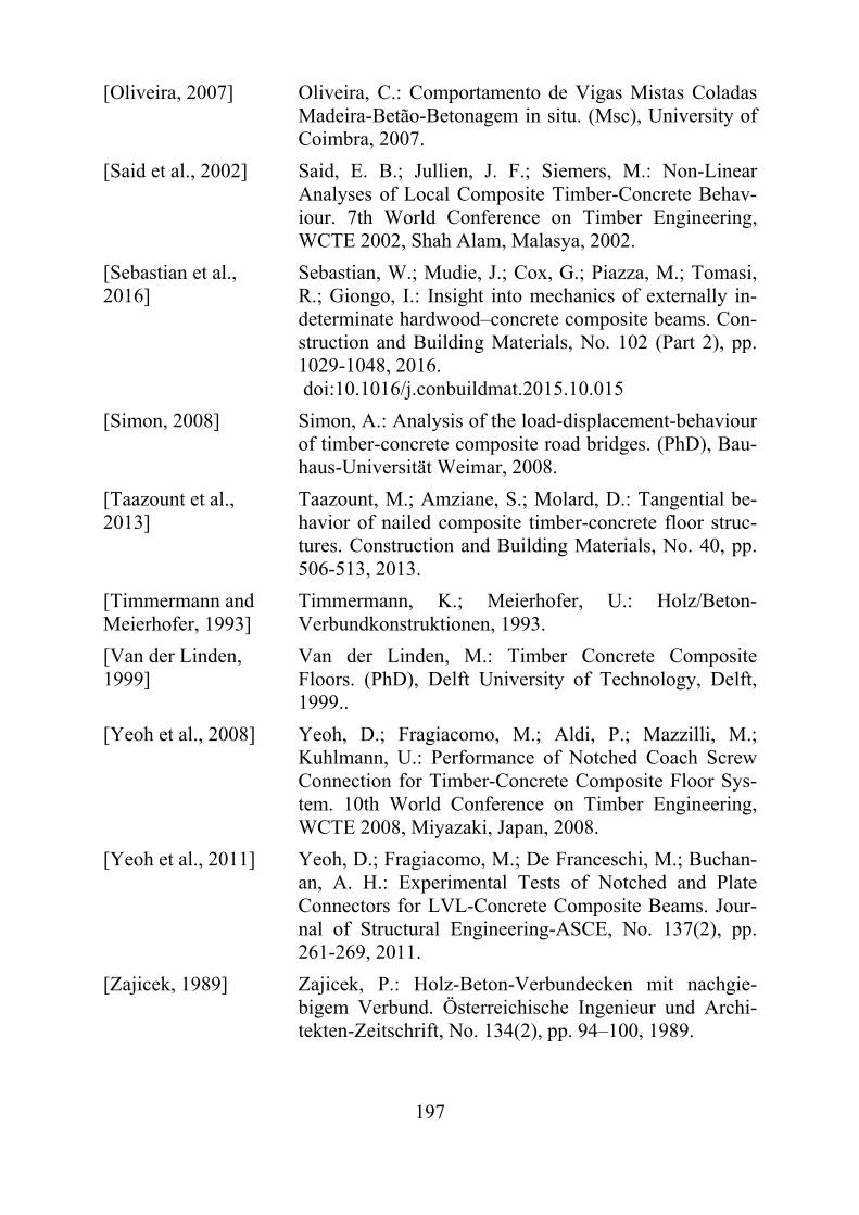
197
[Oliveira, 2007] Oliveira, C.: Comportamento de Vigas Mistas Coladas Madeira-Betão-Betonagem in situ. (Msc), University of Coimbra, 2007.
[Said et al., 2002] Said, E. B.; Jullien, J. F.; Siemers, M.: Non-Linear Analyses of Local Composite Timber-Concrete Behav-iour. 7th World Conference on Timber Engineering, WCTE 2002, Shah Alam, Malasya, 2002.
[Sebastian et al., 2016]
Sebastian, W.; Mudie, J.; Cox, G.; Piazza, M.; Tomasi, R.; Giongo, I.: Insight into mechanics of externally in-determinate hardwood–concrete composite beams. Con-struction and Building Materials, No. 102 (Part 2), pp. 1029-1048, 2016. doi:10.1016/j.conbuildmat.2015.10.015
[Simon, 2008] Simon, A.: Analysis of the load-displacement-behaviour of timber-concrete composite road bridges. (PhD), Bau-haus-Universität Weimar, 2008.
[Taazount et al., 2013]
Taazount, M.; Amziane, S.; Molard, D.: Tangential be-havior of nailed composite timber-concrete floor struc-tures. Construction and Building Materials, No. 40, pp. 506-513, 2013.
[Timmermann and Meierhofer, 1993]
Timmermann, K.; Meierhofer, U.: Holz/Beton-Verbundkonstruktionen, 1993.
[Van der Linden, 1999]
Van der Linden, M.: Timber Concrete Composite Floors. (PhD), Delft University of Technology, Delft, 1999..
[Yeoh et al., 2008] Yeoh, D.; Fragiacomo, M.; Aldi, P.; Mazzilli, M.; Kuhlmann, U.: Performance of Notched Coach Screw Connection for Timber-Concrete Composite Floor Sys-tem. 10th World Conference on Timber Engineering, WCTE 2008, Miyazaki, Japan, 2008.
[Yeoh et al., 2011] Yeoh, D.; Fragiacomo, M.; De Franceschi, M.; Buchan-an, A. H.: Experimental Tests of Notched and Plate Connectors for LVL-Concrete Composite Beams. Jour-nal of Structural Engineering-ASCE, No. 137(2), pp. 261-269, 2011.
[Zajicek, 1989] Zajicek, P.: Holz-Beton-Verbundecken mit nachgie-bigem Verbund. Österreichische Ingenieur und Archi-tekten-Zeitschrift, No. 134(2), pp. 94–100, 1989.

198
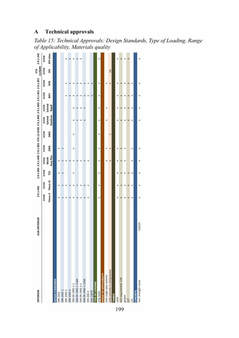
199
A Technical approvals
Table 15: Technical Approvals: Design Standards, Type of Loading, Range of Applicability, Materials quality
CRITER
ION
SUB‐CRITER
ION
Z.9.1‐603Z.9.1‐648Z‐9.1‐803ETA 12‐0196Z‐9.1‐845Z‐9.1‐845Z‐9.1‐851Z‐9.1.857
ETA
13/0699
Z‐9.1‐342
screw
screw
screw
screw
screw
screw
screw
screw
screw
screw
screw
screw
Timco II
Timco III
TCC
Würth
Assy Plus
SWG
SWG
Schmid
Stardrvie
Schmid
Rap
idBiFri
SFIX
SFS
SFS intec
DESIGN STA
NDARDS
DIN 1052
xx
xx
x
DIN 1045‐1
xx
xx
x
DIN 1045‐2
xx
xx
xx
DIN 1045‐3
xx
xx
xx
DIN EN 1995‐1‐1
xx
xx
xx
xx
xx
x
DIN EN 1995‐1‐1\N
Ax
xx
xx
xx
x
DIN EN 1992‐1‐1
xx
xx
xx
xx
DIN EN 1992‐1‐1/N
Ax
xx
xx
xx
DIN 206‐1
xx
xx
x
DIN 13670
xx
TYPE OF LO
ADING
only static
xx
xx
xx
xx
xx
x
RANGE OF APPLICABILITY
only single span
systems
xx
xx
x
only concrete in compression
xx
xx
(x)
TIMBER
solid
xx
xx
xx
xx
xx
min requirem
ent: C24
xx
xx
xx
xx
xx
glulam
xx
xx
xx
xx
xx
CLT
xx
xx
xx
xx
LVL
xx
xx
xx
xx
x
CONCRETE
min. strength classe
C20/25
xx
xx
xx
xx
xx
Z‐9.1‐445
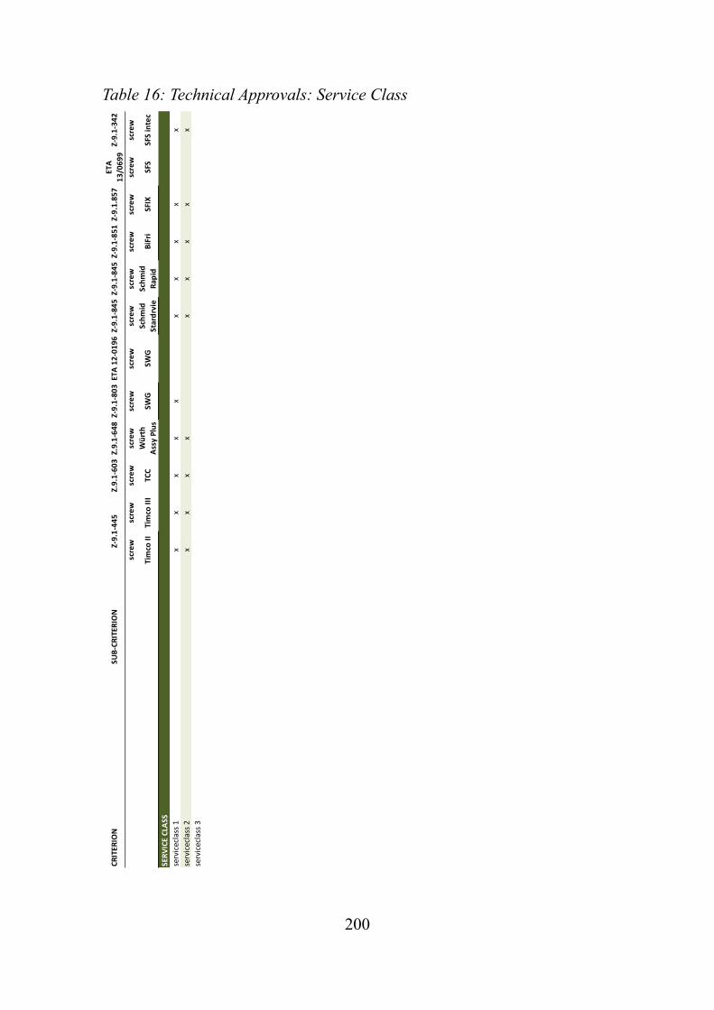
200
Table 16: Technical Approvals: Service Class
CRITER
ION
SUB‐CRITER
ION
Z.9.1‐603Z.9.1‐648Z‐9.1‐803ETA 12‐0196Z‐9.1‐845Z‐9.1‐845Z‐9.1‐851Z‐9.1.857
ETA
13/0699
Z‐9.1‐342
screw
screw
screw
screw
screw
screw
screw
screw
screw
screw
screw
screw
Timco II
Timco III
TCC
Würth
Assy Plus
SWG
SWG
Schmid
Stardrvie
Schmid
Rap
idBiFri
SFIX
SFS
SFS intec
SERVICE CLA
SS
serviceclass 1
xx
xx
xx
xx
xx
serviceclass 2
xx
xx
xx
xx
x
serviceclass 3
Z‐9.1‐445
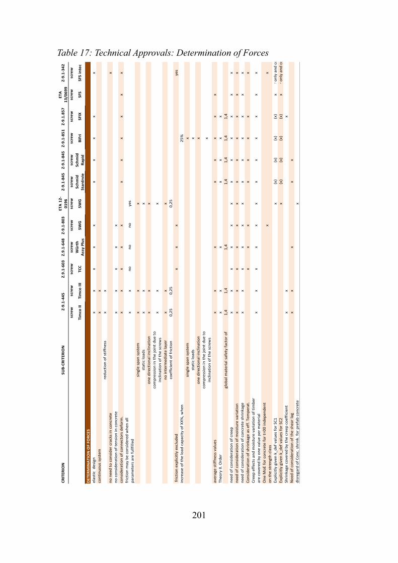
201
Table 17: Technical Approvals: Determination of Forces
CRITERION
SUB‐CRITERION
Z.9.1‐603
Z.9.1‐648
Z‐9.1‐803
ETA 12‐
0196
Z‐9.1‐845
Z‐9.1‐845
Z‐9.1‐851
Z‐9.1.857
ETA
13/0699
Z‐9.1‐342
screw
screw
screw
screw
screw
screw
screw
screw
screw
screw
screw
screw
Tim
co II
Tim
co III
TCC
Würth
Assy Plus
SWG
SWG
Schmid
Stardrvie
Schmid
Rapid
BiFri
SFIX
SFS
SFS intec
DETERMINATION OF FO
RCES
elastic design
xx
xx
xx
xx
xx
continuous system
xx
reduction of stiffness
xx
no need to consider cracks in concrete
x
no consideration of tension in concrete
xx
xx
x
consideration of connectors deform
.x
xx
xx
xx
xx
xx
friction m
ay be considered when all
parameters are fullfilled
xx
no
no
no
yes
single span system
xx
x
static loads
xx
x
one directional inclination
xx
x
compression in the joint due to
inclination of the screws
xx
x
no interm
ediate layer
xx
x
coefficient of friction
0,25
0,25
0,25
friction explicitly excluded
xx
xyes
increase of the load capacity of XX%, when
25%
single span system
x
static loads
x
one directional inclination
x
compression in the joint due to
inclination of the screws
x
average stiffness values
xx
xx
xx
xx
Theory II. Order
xx
xx
xx
x
global material safety factor of
1,4
1,4
1,4
1,4
1,4
1,4
1,4
need of consideration of creep
xx
xx
xx
xx
xx
xx
need of consideration of moisture variation
xx
xx
xx
xx
xx
xx
need of consideration of concrete shrinkage
xx
xx
xx
xx
xx
xx
Consideration of shrinkage as eff. Temperat.
xx
xx
xx
xx
Creep effects and m
oisture variation of timber
are covered by one value per material
xx
xx
xx
xx
xx
xx
One M
oE for concrete for t=00 independent
on the strength class
xx
Explicitly given k_def values for SC1
x(x)
(x)
(x)
(x)
xr only and co
Explicitly given k_def values for SC2
x(x)
(x)
(x)
(x)
xr only and co
Shrinkage covered by the creep coefficient
xx
x
Need of consideration of the shear lag
xx
xx
x
disregard of Conc. shrink. for prefab concrete
x
Z‐9.1‐445
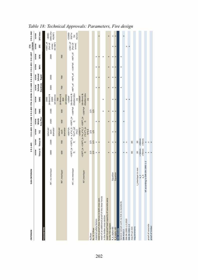
202
Table 18: Technical Approvals: Parameters, Fire design
CRITERION
SUB‐CRITERION
Z.9.1‐603Z.9.1‐648Z‐9.1‐803ETA 12‐0196Z‐9.1‐845Z‐9.1‐845Z‐9.1‐851Z‐9.1.857
ETA
13/0699
Z‐9.1‐342
screw
screw
screw
screw
screw
screw
screw
screw
screw
screw
screw
screw
Tim
co II
Tim
co III
TCC
Würth
Assy Plus
SWG
SWG
Schmid
Stardrvie
Schmid
Rapid
BiFri
SFIX
SFS
SFS intec
PARAMETERS
90°, no interlayer
1800
2200
value per
each
diamater
1500
1500
2000
(d=8mm) &
2400
(d=10mm)
2000
2000
2000
=100 l_ef
(Pair of
screw;
45°/90°)
=8000‐
100ts (for
45/90°)
90°, Interlayer
600
700
value per
each
diamater
500
500
700
(d=8mm) &
800
(d=10mm)
700
700
700
45°, no interlayer
=130*l_{e
f]
=130*l_{e
f]
=400*(rh
o_k*d_1)
^0.2*l_(ef
)^0.4
=100*l_(e
f)=100*lef
=100lef
(ds=8mm) &
45lef(d=10m
m)
=90*l_ef
=90*l_ef
=130*lef
=90*l_Ef
=240 l_ef
(Pair of
screw)
=25000‐
350*ts
for
45/135
45°,interlayer
=130*l_{e
f]
=130*l_{e
f]
=1400*(r
ho_k*d_1
)^0.2*l_(e
f)^0.4
=100*l_(e
f)=100*lef
=100lef
(ds=8mm) &
45lef(d=10m
m)
Ku/Kser
2/3
2/3
2/3
2/3
Ku, SC 2/Kser
2/3
2/3
1/5
2/3
material safety factors
xx
xx
xx
x
need to proof shear forces in both cross sect.
xx
xx
xx
xx
need of an additional proof of the shear forces
in the tim
ber cross section
xx
x
need to proof load capacity of concrete perp
to the TCC‐system
xx
xx
xx
xx
x
R_k, alpha=90
Equation
xx
xx
xx
xx
xx
xx
R_K,alphs =45
Equation
xx
xx
xx
xx
xx
xx
FIRE DESIGN
General remark with no link to standards
xx
xx
DIN 4102‐2
xx
xx
x
DIN EN 1995‐1‐2:2010
xx
xx
DIN EN 1992‐1‐2
xx
max R iun m
in60
60
requierements
t_interlayer in m
m20
20
a_1
> 50mm
>50mm
a_3
>70mm
>70mm
kfi according to DIN EN 1995‐1‐2
xx
proof of concrete
xx
proof of timber
xx
Z‐9.1‐445

203
Table 19: Technical Approvals: Execution CRITERION
SUB‐CRITERION
Z.9.1‐603
Z.9.1‐648
Z‐9.1‐803
ETA 12‐
0196
Z‐9.1‐845
Z‐9.1‐845
Z‐9.1‐851
Z‐9.1.857
ETA
13/0699
Z‐9.1‐342
screw
screw
screw
screw
screw
screw
screw
screw
screw
screw
screw
screw
Tim
co II
Tim
co III
TCC
Würth
Assy Plus
SWG
SWG
Schmid
Stardrvie
Schmid
Rapid
BiFri
SFIX
SFS
SFS intec
EXECUTION
min strength class of timber
C24
C24
C24
C24
C24
C24
C24
C24
C24
C24
CLT, installation in the narrow side
requirement 45°
xx
xx
xx
xx
min strength class of concrete
C20/25
C20/25
C20/25
C20/25
C20/25
C20/25
C20/26
C20/25
C20/25
max diameter of aggregate
16mm
16mm
16mm
16mm
16mm
16mm
16mm
16mm
16mm
16mm
min thickness of concrete
70mm
70mm
70mm
70mm
70mm
70mm
70mm
70mm
70mm
70mm
max thickness of concrete
300mm
300mm
300mm
300mm
300mm
300mm
300mm
300mm
300mm
300mm
Thickness of concrete / thickness of timber
<70%
<70%
<70%
<70%
min thickness of concrete of 60mm when
xx
x
no reinforcement for the shear
xx
xx
xx
xx
no single loads
xx
xx
xx
xx
no linear loads
xx
xx
xx
xx
distance of the beams
<10d_con.<10d_con.<10d_con.<10d_con.<10d_con.
<10d_con.<10d_con.
<10d_con.
min. reinforcement
Q188A
Q188A
Q188
Q188A
Q188A
B500A ‐
150x6 /
B500A ‐
150x6 /
B500A ‐
150x6 /
B500A ‐
150x6 /
Q188
Installation of the reinforcment underneath
the head of the screws
xx
xx
xx
xx
xx
min concrete cover required in the joint
betw
een tim
ber and concrete
xx
xx
xx
xx
xx
additional reinforcement for thicknesses
>100mm
>100mm
>100mm
>100mm
>100mm
>100mm
>100mm
>100mm
>100mm
>100mm
>100mm
additional reinforcement for prefab concrete
elements in conneciton with in situ concrete
xx
xx
xx
x
possibility to install water im
perm
eable layer
xx
xx
xx
requir. to install a water im
perm
eable layer
no
no
no
YES
YES
no
no
no
no
no
possibility to install a interm
ediate layer
xx
xx
xx
xx
x
max thickness of interm
ediate layer
30mm
50mm
50mm
50mm
50mm
50mm
50mm
50mm
50mm
no predrill. required and predrill. not allowed
xx
xx
xx
xx
xx
inlcinations
45° strict
x
inlcinations
>40
x
>45
xx
xx
xx
xx
<50
xx
xx
xx
xx
x
or
>85°
xx
xx
xx
xx
<95
xx
xx
xx
xx
x
minim
um length of the screw in the concrete
50mm
50mm
x
installation in an angle 0f 45°
65mm
65mm
60mm
65mm
installation in an angle of 90°
45mm
45mm
45mm
minim
um coverage of the head of the screw
10mm
10mm
10mm
10mm
minim
um length of the screw in the tim
ber
60mm
installation in an angle of 45°
50mm
installation in an angle of 90°
50mm
only tension in the screw
xx
xx
xx
xx
crossed arrangement
adjustm
ent of the distance of the screws in
dependence on the course of the shear force
xx
xx
xx
xx
xx
max distance
<4min dist.
<4min dist.
<4min dist.
<4min dist.
<4min dist.
<4min dist.
<4min dist.
<4min dist.
<4min dist.
<4min dist.
definition of minim
um spacing
xx
xx
xx
xx
xx
xx
support of the TCC at the tim
ber beam
xx
xx
xx
xx
xx
xx
dry tim
ber (<20%)
xx
xx
xx
xx
xx
propping until sufficient load capacity of
concrete
xx
xx
xx
xx
xx
Z‐9.1‐445

204
205
B Evaluation of the internal forces
B.1 General
In a composite system, the external forces are distributed between the single composite cross section. In cross section with 2 cross sections, the equilibrium of forces is defined by following equation:
⋅
where external bending moment
bending moment in cross section 1
bending moment in cross section 2
normal force in both cross section
distance between the centroids of both cross sections (=inner lever arm)
In principle, the system is statically undetermined, since neither the normal force nor the bending moment can be determined directly. In order to solve it, the strains and curvature in the cross section are used, leading to following equa-tions
Curvature in the single cross section: Assuming the uplift between the single cross sections does not appear, the course of the deformation of the composite elements is equal. Since the curvature is the second derivation of the deformation, the curvature of the single cross section is identical:
Since the bending moment in a cross section depends on the stiffness and the curvature, the bending moment depends on
⋅ ⋅
Strain in the centroid: In principle, the strain in the centroid can be deter-mined by
⋅ However the normal force in the cross sections affects a slip in the joint, which results in a reduced strain in the centroid. This reduced strain can be determined according to EC5 Annex B by
Therefore the normal force in the cross section is determined by
⋅ ⋅ ⋅ , ⋅ ⋅ ⋅
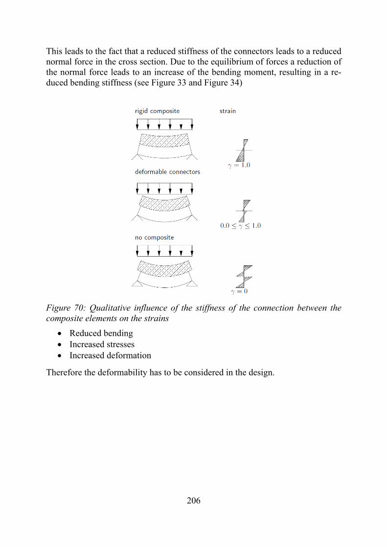
206
This leads to the fact that a reduced stiffness of the connectors leads to a reduced normal force in the cross section. Due to the equilibrium of forces a reduction of the normal force leads to an increase of the bending moment, resulting in a re-duced bending stiffness (see Figure 33 and Figure 34)
Figure 70: Qualitative influence of the stiffness of the connection between the composite elements on the strains
Reduced bending Increased stresses Increased deformation
Therefore the deformability has to be considered in the design.
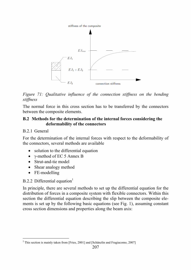
207
Figure 71: Qualitative influence of the connection stiffness on the bending stiffness
The normal force in this cross section has to be transferred by the connectors between the composite elements.
B.2 Methods for the determination of the internal forces considering the deformability of the connectors
B.2.1 General
For the determination of the internal forces with respect to the deformability of the connectors, several methods are available
solution to the differential equation -method of EC 5 Annex B Strut-and-tie model Shear analogy method FE-modelling
B.2.2 Differential equation1
In principle, there are several methods to set up the differential equation for the distribution of forces in a composite system with flexible connectors. Within this section the differential equation describing the slip between the composite ele-ments is set up by the following basic equations (see Fig. 1), assuming constant cross section dimensions and properties along the beam axis:
1 This section is mainly taken from [Fries, 2001] and [Schänzlin and Fragiacomo, 2007]
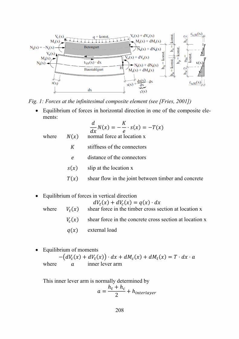
208
Fig. 1: Forces at the infinitesimal composite element (see [Fries, 2001])
Equilibrium of forces in horizontal direction in one of the composite ele-ments:
⋅
where normal force at location x
stiffness of the connectors
distance of the connectors
slip at the location x
shear flow in the joint between timber and concrete
Equilibrium of forces in vertical direction
⋅ where shear force in the timber cross section at location x
shear force in the concrete cross section at location x
external load
Equilibrium of moments ⋅ ⋅ ⋅
where inner lever arm
This inner lever arm is normally determined by
2
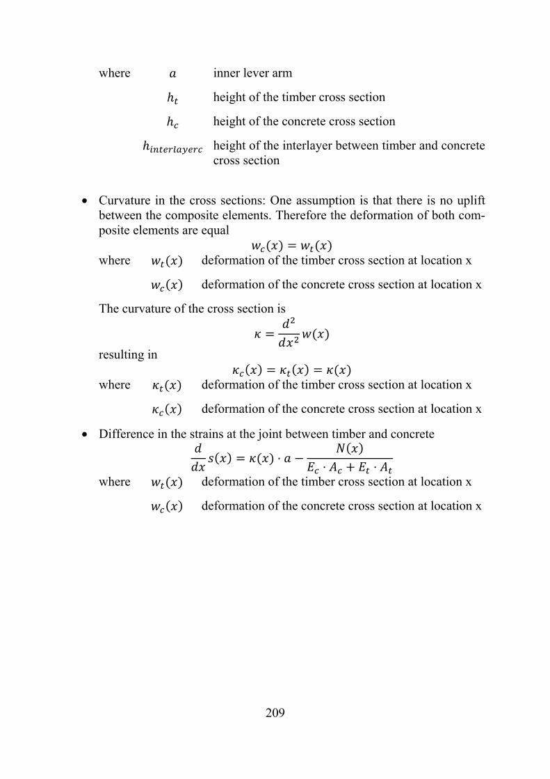
209
where inner lever arm
height of the timber cross section
height of the concrete cross section
height of the interlayer between timber and concrete cross section
Curvature in the cross sections: One assumption is that there is no uplift
between the composite elements. Therefore the deformation of both com-posite elements are equal
where deformation of the timber cross section at location x
deformation of the concrete cross section at location x
The curvature of the cross section is
resulting in
where deformation of the timber cross section at location x
deformation of the concrete cross section at location x
Difference in the strains at the joint between timber and concrete
⋅⋅ ⋅
where deformation of the timber cross section at location x
deformation of the concrete cross section at location x
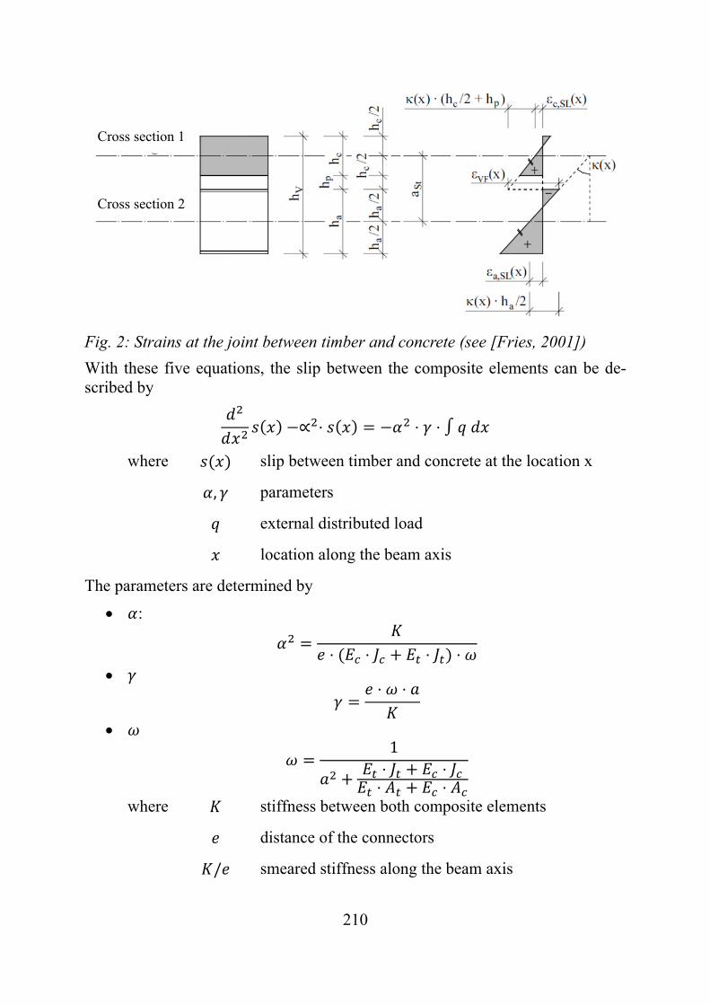
210
Fig. 2: Strains at the joint between timber and concrete (see [Fries, 2001])
With these five equations, the slip between the composite elements can be de-scribed by
∝ ⋅ ⋅ ⋅
where slip between timber and concrete at the location x
, parameters
external distributed load
location along the beam axis
The parameters are determined by
:
⋅ ⋅ ⋅ ⋅
⋅ ⋅
1⋅ ⋅⋅ ⋅
where stiffness between both composite elements
distance of the connectors
/ smeared stiffness along the beam axis
Cross section 1
Cross section 2
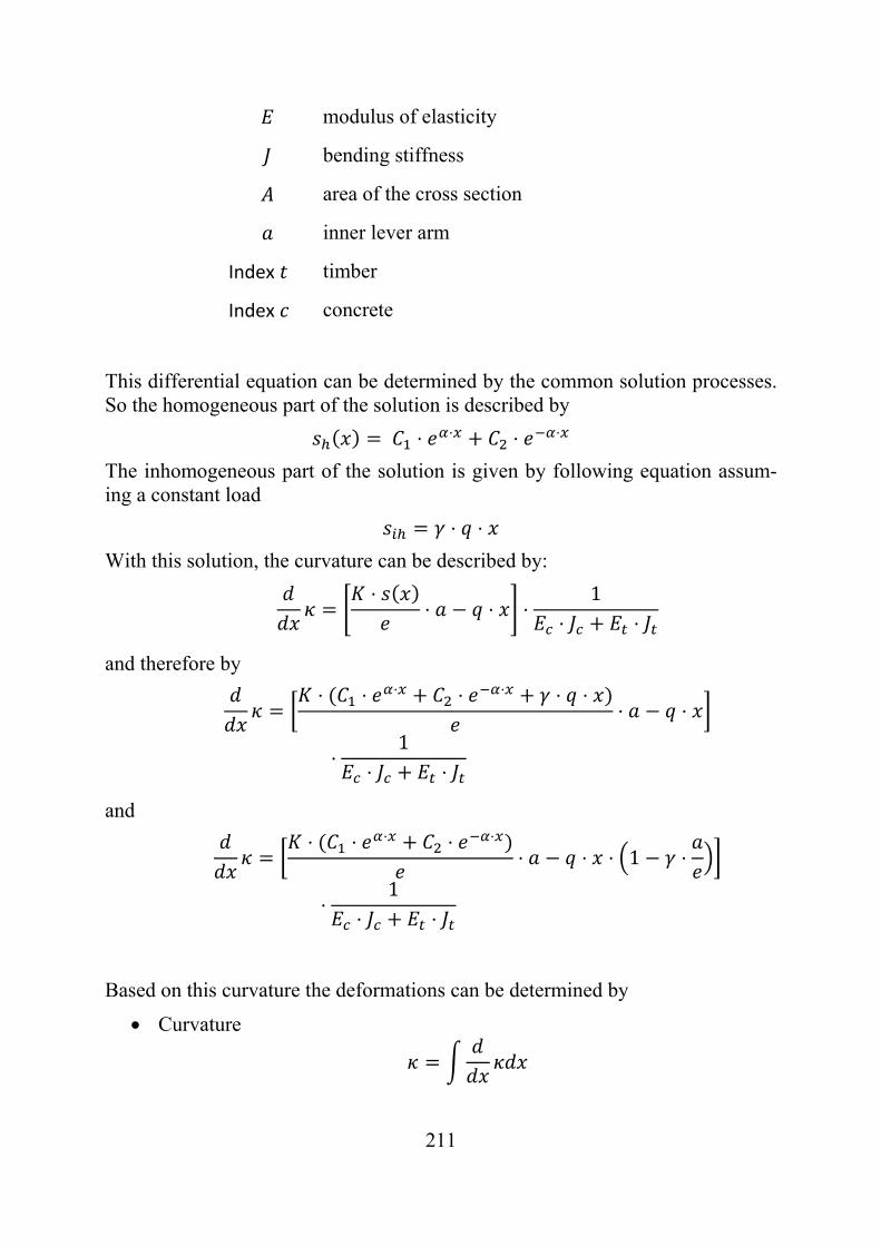
211
modulus of elasticity
bending stiffness
area of the cross section
inner lever arm
Index timber
Index concrete
This differential equation can be determined by the common solution processes. So the homogeneous part of the solution is described by
⋅ ⋅ ⋅ ⋅
The inhomogeneous part of the solution is given by following equation assum-ing a constant load
⋅ ⋅
With this solution, the curvature can be described by:
⋅⋅ ⋅ ⋅
1⋅ ⋅
and therefore by
⋅ ⋅ ⋅ ⋅ ⋅ ⋅ ⋅⋅ ⋅
⋅1
⋅ ⋅
and
⋅ ⋅ ⋅ ⋅ ⋅
⋅ ⋅ ⋅ 1 ⋅
⋅1
⋅ ⋅
Based on this curvature the deformations can be determined by
Curvature
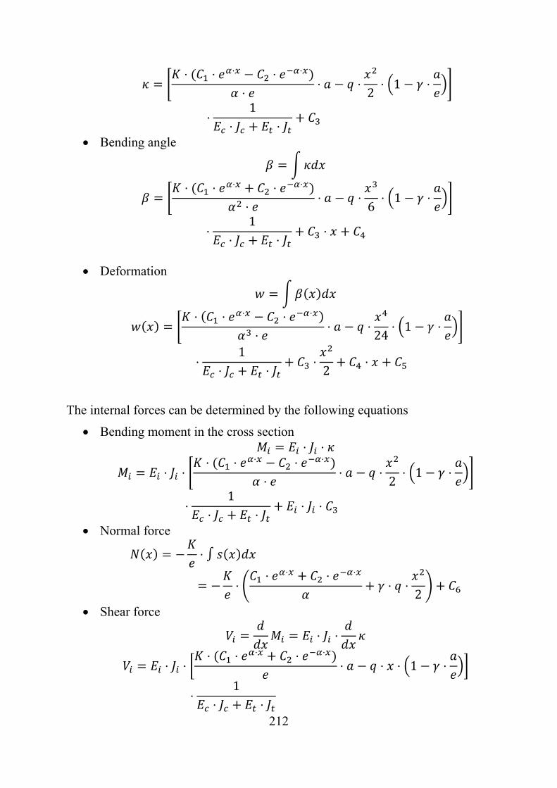
212
⋅ ⋅ ⋅ ⋅ ⋅
⋅⋅ ⋅
2⋅ 1 ⋅
⋅1
⋅ ⋅
Bending angle
⋅ ⋅ ⋅ ⋅ ⋅
⋅⋅ ⋅
6⋅ 1 ⋅
⋅1
⋅ ⋅⋅
Deformation
⋅ ⋅ ⋅ ⋅ ⋅
⋅⋅ ⋅
24⋅ 1 ⋅
⋅1
⋅ ⋅⋅2
⋅
The internal forces can be determined by the following equations
Bending moment in the cross section ⋅ ⋅
⋅ ⋅⋅ ⋅ ⋅ ⋅ ⋅
⋅⋅ ⋅
2⋅ 1 ⋅
⋅1
⋅ ⋅⋅ ⋅
Normal force
⋅
⋅⋅ ⋅ ⋅ ⋅
⋅ ⋅2
Shear force
⋅ ⋅
⋅ ⋅⋅ ⋅ ⋅ ⋅ ⋅
⋅ ⋅ ⋅ 1 ⋅
⋅1
⋅ ⋅
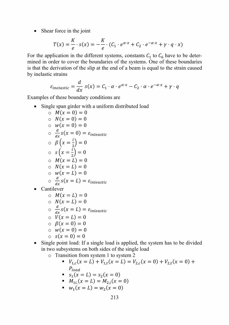
213
Shear force in the joint
⋅ ⋅ ⋅ ⋅ ⋅ ⋅ ⋅ ⋅
For the application in the different systems, constants to have to be deter-mined in order to cover the boundaries of the systems. One of these boundaries is that the derivation of the slip at the end of a beam is equal to the strain caused by inelastic strains
⋅ ⋅ ⋅ ⋅ ⋅ ⋅ ⋅
Examples of these boundary conditions are
Single span girder with a uniform distributed load o 0 0 o 0 0 o 0 0
o 0
o 0
o 0
o 0 o 0 o 0
o
Cantilever o 0 o 0
o
o 0 o 0 0 o 0 0 o 0 0
Single point load: If a single load is applied, the system has to be divided in two subsystems on both sides of the single load
o Transition from system 1 to system 2 , , , 0 , 0
0 , , 0 0
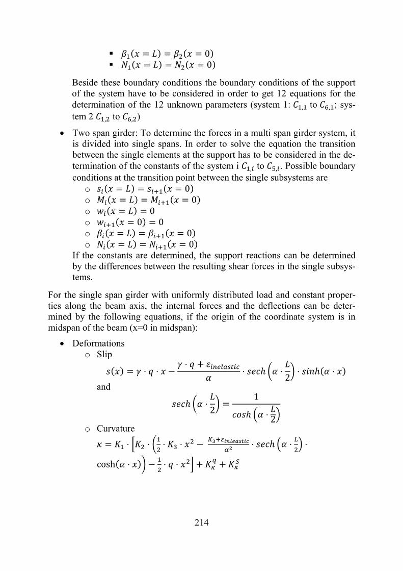
214
0 0
Beside these boundary conditions the boundary conditions of the support of the system have to be considered in order to get 12 equations for the determination of the 12 unknown parameters (system 1: , to , ; sys-tem 2 , to , )
Two span girder: To determine the forces in a multi span girder system, it is divided into single spans. In order to solve the equation the transition between the single elements at the support has to be considered in the de-termination of the constants of the system i , to , . Possible boundary conditions at the transition point between the single subsystems are
o 0 o 0 o 0 o 0 0 o 0 o 0
If the constants are determined, the support reactions can be determined by the differences between the resulting shear forces in the single subsys-tems.
For the single span girder with uniformly distributed load and constant proper-ties along the beam axis, the internal forces and the deflections can be deter-mined by the following equations, if the origin of the coordinate system is in midspan of the beam (x=0 in midspan):
Deformations o Slip
⋅ ⋅⋅
⋅ ⋅2
⋅ ⋅
and
⋅2
1
⋅ 2
o Curvature
⋅ ⋅ ⋅ ⋅ ⋅ ⋅ ⋅
cosh ⋅ ⋅ ⋅

215
and
1
⋅ ⋅
⋅
⋅
⋅ ⋅18⋅ ⋅
18⋅ ⋅
⋅ ⋅
o Bending angle
⋅ ⋅ ⋅ ⋅ ⋅ ⋅ ⋅
sinh ⋅ ⋅ ⋅ ⋅
o Deflection
⋅ ⋅ ⋅ ⋅ ⋅ ⋅ ⋅
cosh ⋅ ⋅ ⋅ ⋅ ⋅
and
⋅ ⋅1384
⋅ ⋅1384
⋅ ⋅18⋅ ⋅
⋅ ⋅ ⋅1
8
Forces
o Shear forces in the joint
⋅ ⋅ ⋅⋅
⋅ ⋅ ⋅ sinh ⋅
o Normal force in the timber cross section
⋅ ⋅ ⋅ ⋅⋅
⋅ ⋅ ⋅
cosh ⋅
and
⋅18⋅ ⋅ ⋅
⋅
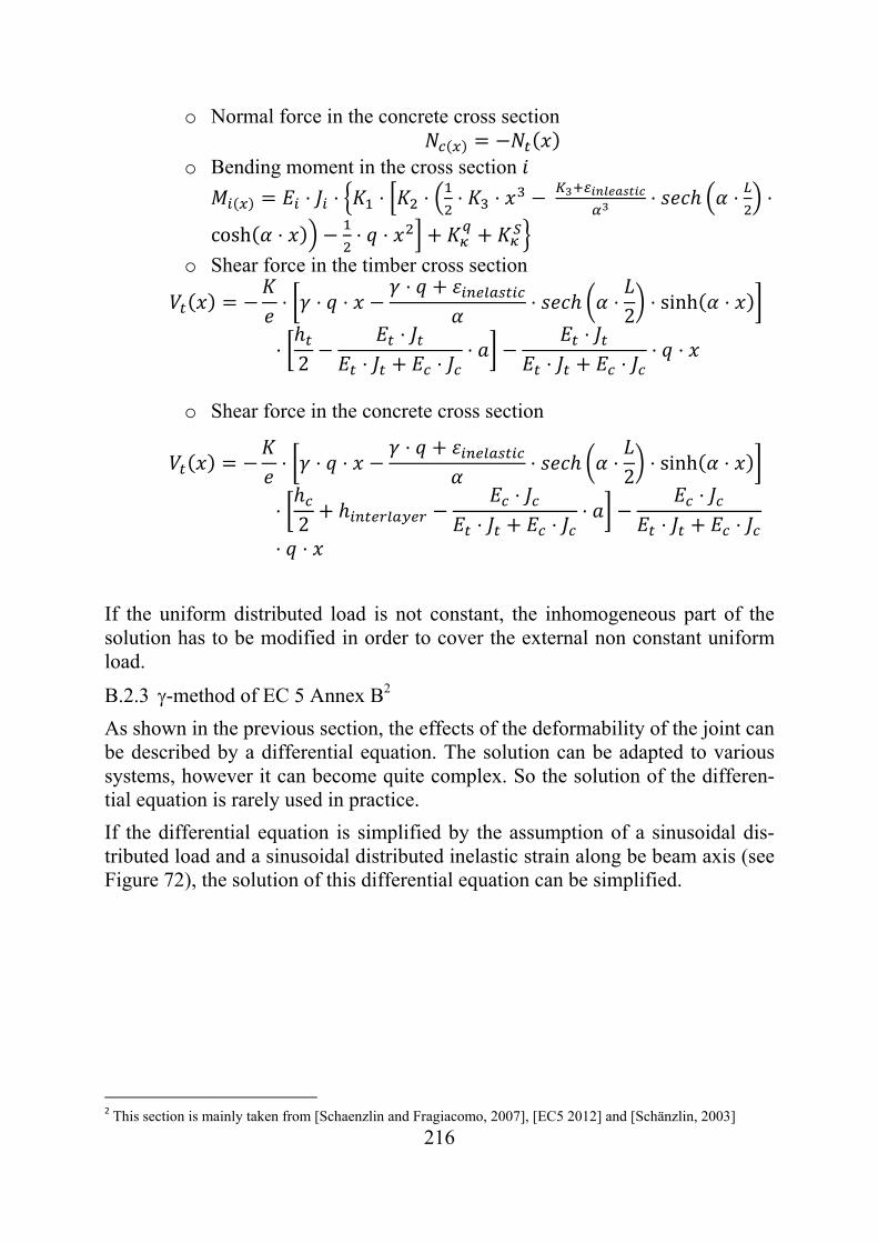
216
o Normal force in the concrete cross section
o Bending moment in the cross section
⋅ ⋅ ⋅ ⋅ ⋅ ⋅ ⋅ ⋅ ⋅
cosh ⋅ ⋅ ⋅
o Shear force in the timber cross section
⋅ ⋅ ⋅⋅
⋅ ⋅2
⋅ sinh ⋅
⋅2
⋅⋅ ⋅
⋅⋅
⋅ ⋅⋅ ⋅
o Shear force in the concrete cross section
⋅ ⋅ ⋅⋅
⋅ ⋅2
⋅ sinh ⋅
⋅2
⋅⋅ ⋅
⋅⋅
⋅ ⋅⋅ ⋅
If the uniform distributed load is not constant, the inhomogeneous part of the solution has to be modified in order to cover the external non constant uniform load.
B.2.3 -method of EC 5 Annex B2
As shown in the previous section, the effects of the deformability of the joint can be described by a differential equation. The solution can be adapted to various systems, however it can become quite complex. So the solution of the differen-tial equation is rarely used in practice.
If the differential equation is simplified by the assumption of a sinusoidal dis-tributed load and a sinusoidal distributed inelastic strain along be beam axis (see Figure 72), the solution of this differential equation can be simplified.
2 This section is mainly taken from [Schaenzlin and Fragiacomo, 2007], [EC5 2012] and [Schänzlin, 2003]
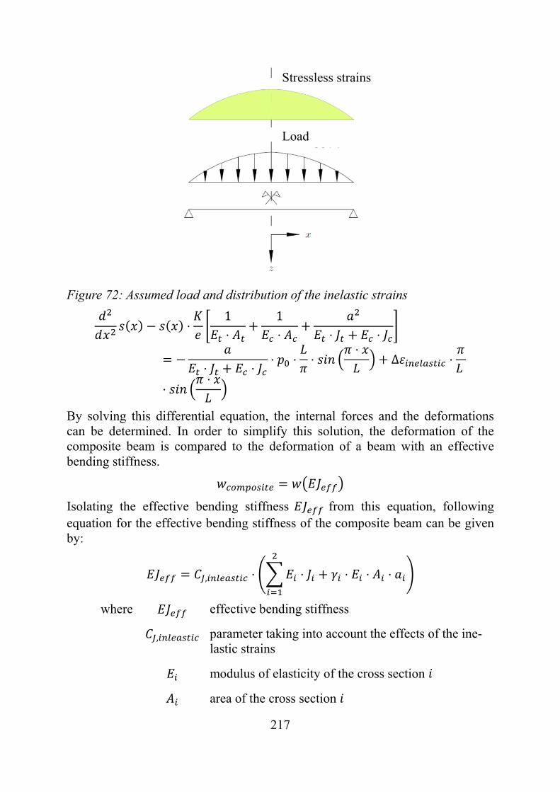
217
Figure 72: Assumed load and distribution of the inelastic strains
⋅1⋅
1⋅ ⋅ ⋅
⋅ ⋅⋅ ⋅ ⋅
⋅Δ ⋅
⋅⋅
By solving this differential equation, the internal forces and the deformations can be determined. In order to simplify this solution, the deformation of the composite beam is compared to the deformation of a beam with an effective bending stiffness.
Isolating the effective bending stiffness from this equation, following equation for the effective bending stiffness of the composite beam can be given by:
, ⋅ ⋅ ⋅ ⋅ ⋅
where effective bending stiffness
, parameter taking into account the effects of the ine-lastic strains
modulus of elasticity of the cross section
area of the cross section
Stressless strains
Load
218
moment of inertia of the cross section
parameter taking into account the effect of the de-formability of the connectors
effective lever arm
= distance between the centroid of the composite cross section to the centroid of the single cross sec-tion
The -value can be determined by
1
1⋅ ⋅ ⋅
⋅
and
1
This parameter can also be expressed by the ratio between the strain in the cen-troid of the cross section 1 for deformable connectors and for rigid connectors subjected to the same curvature
, ,
, ,
So this value can vary between 0 (=no composite) to 1,0 (=rigid connection). Therefore, it is an indicator of the effectiveness of the chosen connection.
The inner lever arm of the single cross section can be determined by
⋅ ⋅⋅ ⋅ ⋅ ⋅
⋅2
and
2 2
Since inelastic strains modifies the loading of the connectors, the effective bend-ing stiffness has to be modified by the factor ,
, ⋅ ⋅⋅ ⋅ ⋅ ⋅
In order to consider the effects of inelastic strains, an external fictitious load can be applied on the system by
, ⋅ Δ
219
where
, ⋅⋅ ⋅ ⋅ ⋅ ⋅⋅ ⋅ ⋅
2
and
Δ
The deformation and the internal forces are determined as follows:
Deformation ;
For a single span girder, the deformation can be determined by
5384
⋅ ⋅
Bending moment ⋅
⋅ 0.8 ⋅
For a single span girder this equation turns into ⋅
⋅ 0.8 ⋅ ⋅8
Normal force: The normal force is influenced by the inelastic strains.
However these inelastic strains lead to eigenstresses. Therefore the ficti-tious loads covering the inelastic strains as shrinkage would lead to an in-crease of the normal force although shrinkage leads to a decrease of the normal force (see Figure 35). Consequently the normal force can be de-termined by the equilibrium of forces by
0.8 ⋅ 0.8 ⋅
2 2
The normal force in the concrete cross section can be determined by
Effective shear force for the determination of the shear stresses in the cross section and the shear stresses in the connection
o Shortening of the cross section 1 related to the cross section 2
⋅ ⋅ ⋅⋅ ⋅
⋅ ⋅ ⋅ ⋅ ⋅⋅ Δ
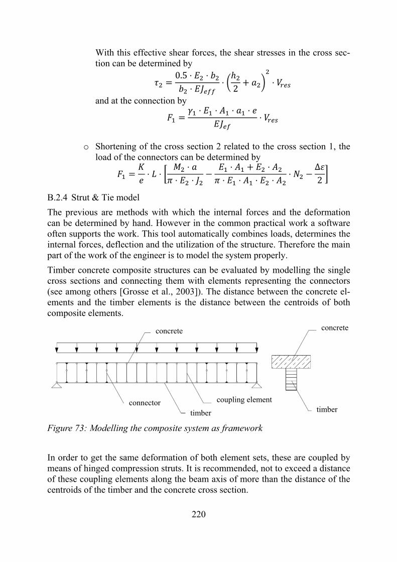
220
With this effective shear forces, the shear stresses in the cross sec-tion can be determined by
0.5 ⋅ ⋅⋅
⋅2
⋅
and at the connection by ⋅ ⋅ ⋅ ⋅
⋅
o Shortening of the cross section 2 related to the cross section 1, the
load of the connectors can be determined by
⋅ ⋅⋅
⋅ ⋅⋅ ⋅
⋅ ⋅ ⋅ ⋅⋅
Δ2
B.2.4 Strut & Tie model
The previous are methods with which the internal forces and the deformation can be determined by hand. However in the common practical work a software often supports the work. This tool automatically combines loads, determines the internal forces, deflection and the utilization of the structure. Therefore the main part of the work of the engineer is to model the system properly.
Timber concrete composite structures can be evaluated by modelling the single cross sections and connecting them with elements representing the connectors (see among others [Grosse et al., 2003]). The distance between the concrete el-ements and the timber elements is the distance between the centroids of both composite elements.
Figure 73: Modelling the composite system as framework
In order to get the same deformation of both element sets, these are coupled by means of hinged compression struts. It is recommended, not to exceed a distance of these coupling elements along the beam axis of more than the distance of the centroids of the timber and the concrete cross section.
concrete concrete
timber timber connector coupling element
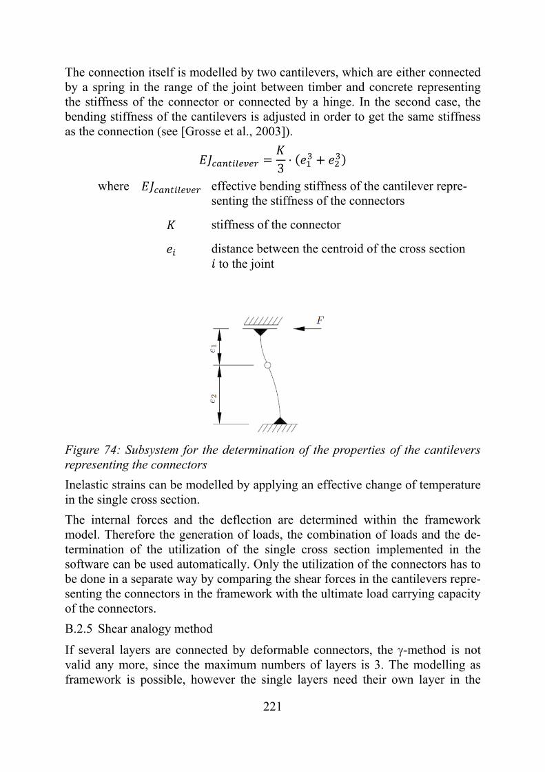
221
The connection itself is modelled by two cantilevers, which are either connected by a spring in the range of the joint between timber and concrete representing the stiffness of the connector or connected by a hinge. In the second case, the bending stiffness of the cantilevers is adjusted in order to get the same stiffness as the connection (see [Grosse et al., 2003]).
3⋅
where effective bending stiffness of the cantilever repre-senting the stiffness of the connectors
stiffness of the connector
distance between the centroid of the cross section to the joint
Figure 74: Subsystem for the determination of the properties of the cantilevers representing the connectors
Inelastic strains can be modelled by applying an effective change of temperature in the single cross section.
The internal forces and the deflection are determined within the framework model. Therefore the generation of loads, the combination of loads and the de-termination of the utilization of the single cross section implemented in the software can be used automatically. Only the utilization of the connectors has to be done in a separate way by comparing the shear forces in the cantilevers repre-senting the connectors in the framework with the ultimate load carrying capacity of the connectors.
B.2.5 Shear analogy method
If several layers are connected by deformable connectors, the -method is not valid any more, since the maximum numbers of layers is 3. The modelling as framework is possible, however the single layers need their own layer in the
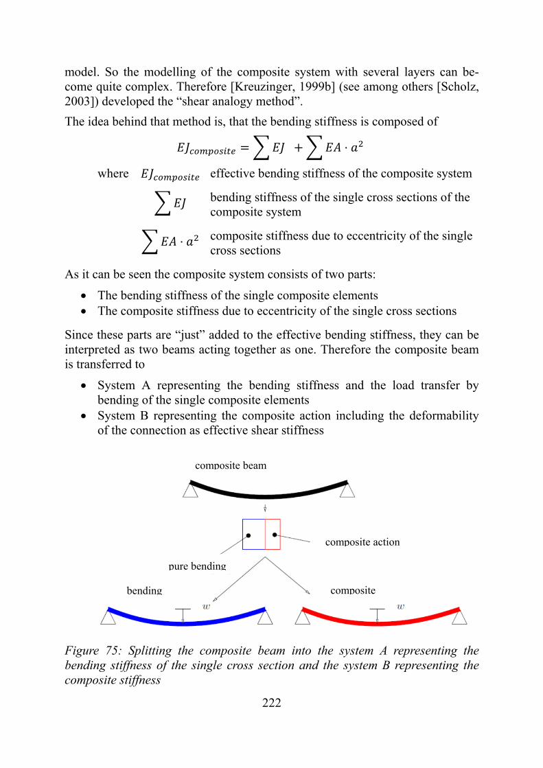
222
model. So the modelling of the composite system with several layers can be-come quite complex. Therefore [Kreuzinger, 1999b] (see among others [Scholz, 2003]) developed the “shear analogy method”.
The idea behind that method is, that the bending stiffness is composed of
⋅
where effective bending stiffness of the composite system
bending stiffness of the single cross sections of the composite system
⋅ composite stiffness due to eccentricity of the single cross sections
As it can be seen the composite system consists of two parts:
The bending stiffness of the single composite elements The composite stiffness due to eccentricity of the single cross sections
Since these parts are “just” added to the effective bending stiffness, they can be interpreted as two beams acting together as one. Therefore the composite beam is transferred to
System A representing the bending stiffness and the load transfer by bending of the single composite elements
System B representing the composite action including the deformability of the connection as effective shear stiffness
Figure 75: Splitting the composite beam into the system A representing the bending stiffness of the single cross section and the system B representing the composite stiffness
composite beam
composite action
pure bending
composite bending
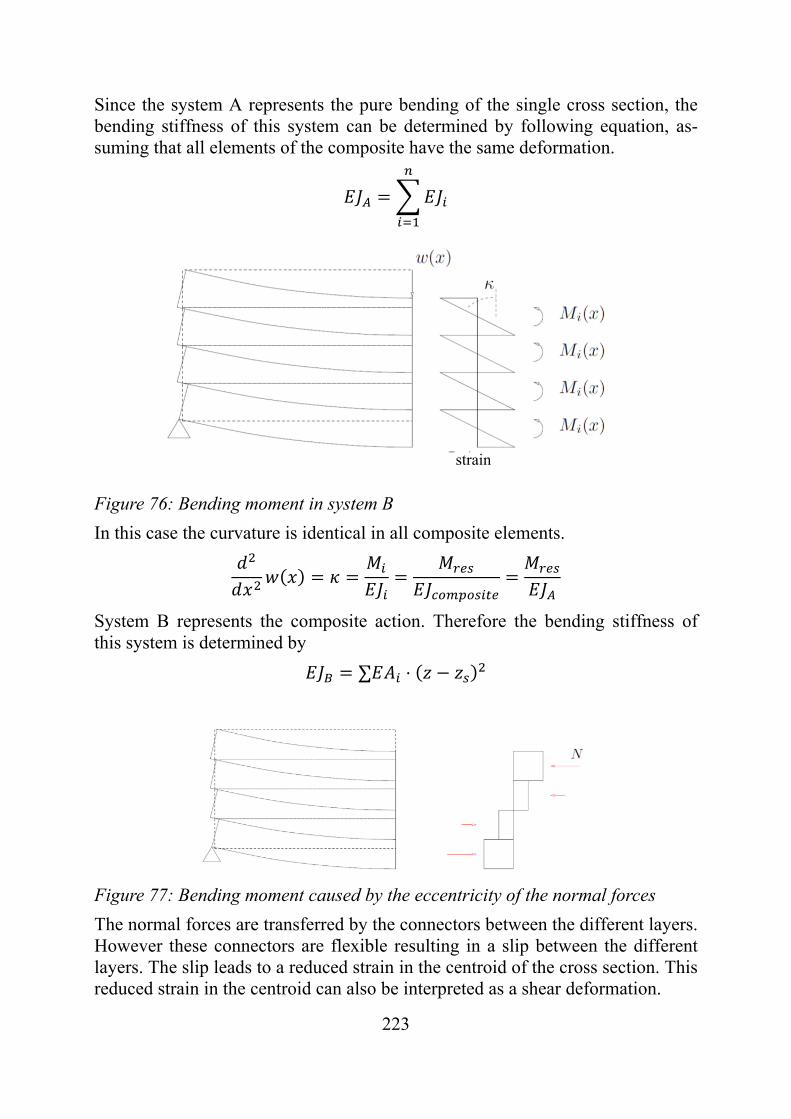
223
Since the system A represents the pure bending of the single cross section, the bending stiffness of this system can be determined by following equation, as-suming that all elements of the composite have the same deformation.
Figure 76: Bending moment in system B
In this case the curvature is identical in all composite elements.
System B represents the composite action. Therefore the bending stiffness of this system is determined by
∑ ⋅
Figure 77: Bending moment caused by the eccentricity of the normal forces
The normal forces are transferred by the connectors between the different layers. However these connectors are flexible resulting in a slip between the different layers. The slip leads to a reduced strain in the centroid of the cross section. This reduced strain in the centroid can also be interpreted as a shear deformation.
strain
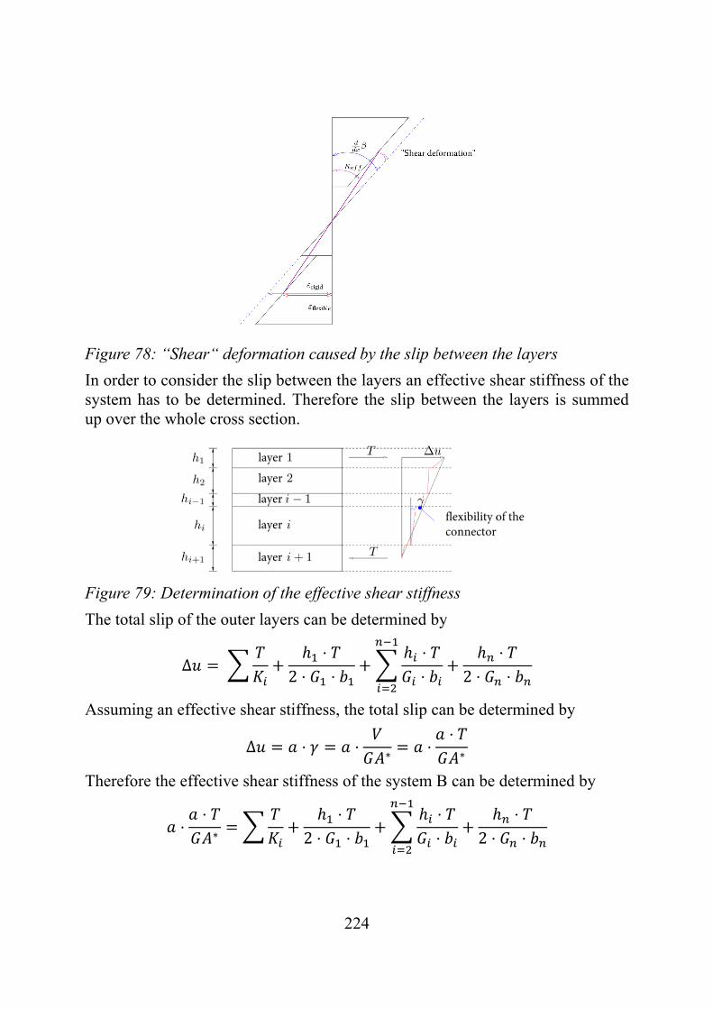
224
Figure 78: “Shear“ deformation caused by the slip between the layers
In order to consider the slip between the layers an effective shear stiffness of the system has to be determined. Therefore the slip between the layers is summed up over the whole cross section.
Figure 79: Determination of the effective shear stiffness
The total slip of the outer layers can be determined by
Δ ⋅
2 ⋅ ⋅⋅⋅
⋅2 ⋅ ⋅
Assuming an effective shear stiffness, the total slip can be determined by
Δ ⋅ ⋅ ∗ ⋅⋅∗
Therefore the effective shear stiffness of the system B can be determined by
⋅⋅∗
⋅2 ⋅ ⋅
⋅⋅
⋅2 ⋅ ⋅
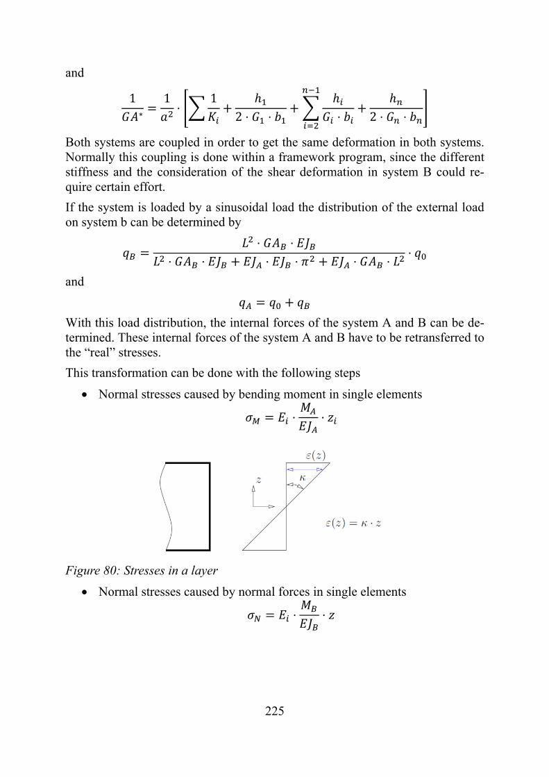
225
and
1∗
1⋅
12 ⋅ ⋅ ⋅ 2 ⋅ ⋅
Both systems are coupled in order to get the same deformation in both systems. Normally this coupling is done within a framework program, since the different stiffness and the consideration of the shear deformation in system B could re-quire certain effort.
If the system is loaded by a sinusoidal load the distribution of the external load on system b can be determined by
⋅ ⋅⋅ ⋅ ⋅ ⋅ ⋅ ⋅
⋅
and
With this load distribution, the internal forces of the system A and B can be de-termined. These internal forces of the system A and B have to be retransferred to the “real” stresses.
This transformation can be done with the following steps
Normal stresses caused by bending moment in single elements
⋅ ⋅
Figure 80: Stresses in a layer
Normal stresses caused by normal forces in single elements
⋅ ⋅
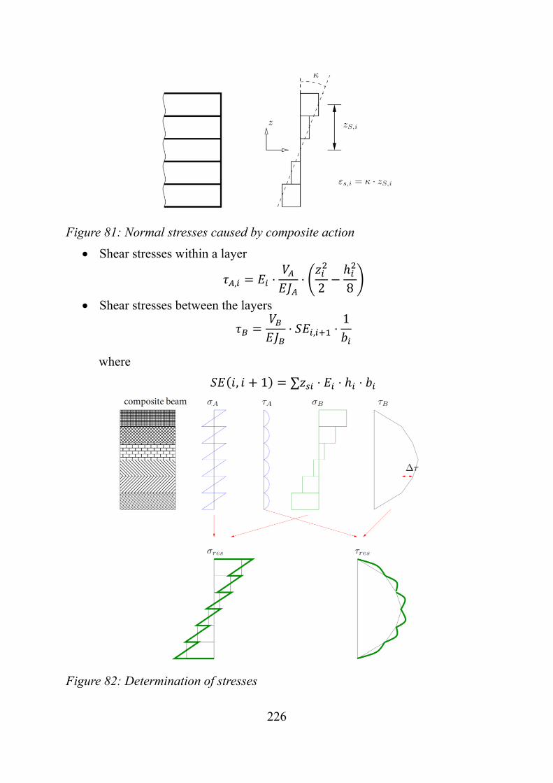
226
Figure 81: Normal stresses caused by composite action
Shear stresses within a layer
, ⋅ ⋅2 8
Shear stresses between the layers
⋅ , ⋅1
where
, 1 ∑ ⋅ ⋅ ⋅
Figure 82: Determination of stresses
227
In order to consider the inelastic strains, these are transferred into a bending moment and a normal force by
Normal force , ⋅ ⋅ Δ
where normal force due to inelastic strain
modulus of the layer with the inelastic strain
area of the layer with the inelastic strain
Δ inelastic strain
Bending moment
, ⋅
where bending moment in the System B
normal force due to inelastic strain
inner cantilever
which are applied to system B, since this system represents the composite ac-tion.
In order to determine the resulting normal forces in the layer, the normal forces caused by inelastic strains have to be superposed with the normal forces in the layers of the system B.
B.2.6 FE-modelling
In principle, the modelling of composite systems with means of Finite-Elements is possible. The advantage of this procedure is that it enables a modelling with very few simplifications. So shear deformations can be considered or the load transfer in the range of the connector can be modelled in a more precise way than the other methods. However, this more precise description of the stresses and deformations need a larger effort in modelling and calculation of the com-posite systems. So the range of application of FE-is more in the range of re-search and development, than in the practical design process of buildings.
228
B.2.7 Summary
For the design of timber-concrete-composite systems several methods can be applied. These methods differ in the range of application, the effort in the appli-cation and therefore in the time needed. Comparing these different methods the -method according to EC5 Annex B and the modelling as frame work system seem to be the most practical methods for the design process.
The -method has the advantage, that it can be solved by hand, but has the limi-tations, that it can only model single span systems with smeared connectors and uniformly distributed loads. In difference to this method, the modelling as framework allows to take into account different structural systems, point loads or discrete distributed connectors. However it has the disadvantage, that a soft-ware tool for solving the framework is necessary.


![Light Steel-Timber Frame with Composite and Plaster ... · Light Steel-Timber Frame with Composite and Plaster Bracing Panels Roberto Scotta:, ... [26] is stapled to the timber frame,](https://img.pdfslide.us/doc/110x75/5e8511d690da694c246c0195/light-steel-timber-frame-with-composite-and-plaster-light-steel-timber-frame.jpg)