Embed Size (px)
Citation preview

UNIVERSITY OF NAIROBI
DEPARTMENT OF ENVIRONMENTAL AND BIOSYSTEMS ENGINEERING
ENGINEERING DESIGN PROJECT (FEB 540)
DESIGN OF SURFACE IRRIGATION SYSTEM
(THAANA NZAU LOCATION)
DESIGNED BY: KHAEMBA LILIAN NEKESA
REG. NO: F21/0039/2008
Project submitted in partial fulfillment of Bachelor of Science in Environmental and
Biosystems engineering
APRIL 2013
SUPERVISOR: MR. J.P. OBIERO
DATE OF SUBMISSION: 3RD
MAY, 2013

F21/0039/2008
Page ii
Declaration
This project is my original work and has never been submitted to any university or
institution for award of honors or any other purpose. I therefore do submit it for evaluation
and consequent award of Bachelor of Science degree in Environmental and Biosystems
Engineering.
Khaemba Lilian Nekesa
Signature Date
…………………………………………………………………………..
J.P Obiero: Supervisor
Signature Date
……………….......................................................................................

F21/0039/2008
Page ii
Acknowledgement
The fundamental of this design project was based on Water and Irrigation courses and I thank my
Lecturers for presenting the concepts.
I thank my supervisor Mr. J.P Obiero for the tireless engagement and critics which made the
project a success.
I also thank Miss Ochengo of Bhundia Associates for teaching me how to design a surface
irrigation system.
I thank the Almighty God for the sufficient grace to finish the project.

F21/0039/2008
Page iii
ABSTRACT
The project is about the design of a surface irrigation system in Thaana Nzau location. The area
receives little rainfall as evident from Mwingi Metrological station. As a result, the area has a low
agricultural productivity. The area has the perennial river Tana which has not been fully utilized
due to lack of suitable skills and technology to supplement the farming. The area has been
divided into 5 units. For the design of the canals an area of 10 Ha for 20 farmers was used, each
with an irrigable plot of 0.55 Ha.
The crop water requirements of the common crops grown in the area were estimated using the
Penman Monteith equation which is incorporated in CROPWAT and CLIMWAT software. The
layout of the area was digitized using Global Mapper and AutoCAD. The design of canals was
done using the Manning’s equation. Other software used was Haestad Hydraulic Applications –
Flow master for estimation of the canal bed width and depth, Spreadsheet for iteration process
and Liscad for canal shape.
Upon the implementation of the project, there will be sufficient water for irrigation and domestic
use, improved agricultural productivity, living standards and employment opportunities.
F21/0039/2008
Page iv
Table of Contents
Declaration ................................................................................................................................... ii
Acknowledgement ....................................................................................................................... ii
ABSTRACT ............................................................................................................................... iii
Table of Contents ......................................................................................................................... iv
LIST OF EQUATIONS ............................................................................................................. vii
1.0 INTRODUCTION ................................................................................................................................... 8
1.1 Statement of the problem and problem analysis ..................................................................... 8
1.2 Site Analysis and inventory .................................................................................................... 2
1.2.1 Population ..................................................................................................................................... 2
1.2.2 Climate ......................................................................................................................................... 2
1.2.3 Topography .................................................................................................................................. 2
1.2.4 Water Resources ........................................................................................................................... 3
1.2.5 Soils .............................................................................................................................................. 3
1.3 Overall objectives ................................................................................................................... 4
1.3.1 Specific Objectives ....................................................................................................................... 4
1.4 Statement of Scope ................................................................................................................. 4
2.0 LITERATURE REVIEW ........................................................................................................................ 5
2.2 Surface irrigation .................................................................................................................... 6
2.3 Components of a surface irrigation system ............................................................................ 7
2.3.1 The water source........................................................................................................................... 7
F21/0039/2008
Page v
2.3.2 The intake facilities ...................................................................................................................... 7
2.3.3 The conveyance system ................................................................................................................ 7
2.3.4 The field canal and/or pipe system ............................................................................................... 7
2.3.5 The infield water use system ........................................................................................................ 9
2.3.6 The drainage system ..................................................................................................................... 9
2.3.7 Accessibility infrastructure ........................................................................................................... 9
2.4 Design of Scheme Layout ....................................................................................................... 9
2.5 Crop Water Requirement ...................................................................................................... 11
3.0 THEORETICAL FRAMEWORK......................................................................................................... 13
3.1 Penman-Monteith equation ................................................................................................... 13
3.2 Crop coefficient approach .................................................................................................... 14
3.3 Crop factor (Kc) .................................................................................................................... 14
3.4 Net Irrigation Requirement (NIR) ........................................................................................ 15
3.5 Gross Irrigation Requirement, GIR ...................................................................................... 15
3.6 Project Water Requirement (PWR) ...................................................................................... 16
3.7 Design command area .......................................................................................................... 16
3.8 Canal Design ......................................................................................................................... 16
3.8.1 Side slope, Z ............................................................................................................................... 19
3.8.2 Velocity, V ................................................................................................................................. 20
3.8.3 The water depth, b and bed width, d ratio .................................................................................. 20
3.8.4 Freeboard .................................................................................................................................... 20
Pipeline Flow Hydraulics .................................................................................................................... 20
3.8.1 Use of Manning Formula Charts ................................................................................................ 21
3.8.3 Use of commercial computer software ....................................................................................... 22
4.0 METHODOLOGY .......................................................................................................................... 23
4.1 The area of study .................................................................................................................. 23
F21/0039/2008
Page vi
4.2 Estimation of crop water requirements ................................................................................. 23
4.2.1 CROPWAT procedure: .............................................................................................................. 24
4.2.2 Net Irrigation Requirement (NIR) .............................................................................................. 24
4.3. Canal design ................................................................................................................................. 25
4.3.1 Determination of system layout ......................................................................................... 25
Layout Procedure ................................................................................................................................ 25
4.3.2 Profile Generation ...................................................................................................................... 25
4.3.5 Profile generation in cad ............................................................................................................. 32
4.3.6 Drain design ............................................................................................................................... 34
4.3.6 Hydraulic structures.................................................................................................................... 35
4.3.7 Culverts ...................................................................................................................................... 35
4.3.8 Regulation structures .................................................................................................................. 36
Measuring structures ........................................................................................................................... 38
4.3.9 Other structures .......................................................................................................................... 38
5.0 RESULTS AND DISCUSSION...................................................................................................... 40
5.1 Crop Water Requirement ...................................................................................................... 40
5.1.1 Reference Crop Evapotranspiration, ETo ................................................................................... 40
5.1.2 Net Irrigation Requirement (NIR) .............................................................................................. 48
Determination of the overhead Tank capacity ..................................................................................... 48
5.2 Canals Discharges ................................................................................................................. 49
7.0 BILL OF QUANTITIES ................................................................................................................. 57
8.0 CONCLUSION ..................................................................................................................................... 58
9.0 RECOMMENDATION ......................................................................................................................... 58
10.0 REFERENCES ............................................................................................................................ 59
11.0 APENDIX .............................................................................................................................................. I
11.1 PICTURES .................................................................................................................... I
11.2 LOCATION MAP ............................................................................................................... II
11.3 CANAL LAYOUT .............................................................................................................. II
F21/0039/2008
Page vii
11.4 SOIL MAP ........................................................................................................................... II
11.5 CONVEYANCE CANAL PROFILE (3 PARTS)............................................................... II
11.6 SUB MAIN 5 PROFILE (2 PARTS) .................................................................................. II
11.7 FEEDER 2-1 PROFILE ....................................................................................................... II
LIST OF EQUATIONS
Equation 1: Penman-Monteith equation ........................................................................................ 13
Equation 2: crop evapo-transpiration ............................................................................................ 14
Equation 3: NIR ............................................................................................................................ 15
Equation 4: GIR ............................................................................................................................ 15
Equation 5: Project water requirement .......................................................................................... 16
Equation 6: Manning’s .................................................................................................................. 17
Equation 7: Wetted perimeter ....................................................................................................... 18
Equation 8: Hydraulic radius ......................................................................................................... 18
Equation 9: Froude no. .................................................................................................................. 18
Equation 10: Hazen- Williams ...................................................................................................... 21
F21/0039/2008
Page viii
Chapter 1
1.0 INTRODUCTION
In every region of the world it is necessary to find or develop appropriate techniques for
agriculture. A large part of the surface of the world is arid, characterized as too dry for
conventional rain fed agriculture. Yet, millions of people live in such regions, and if current
trends in population increase continue, there will soon be millions more. These people must eat,
and the wisest course for them is to produce their own food(Frankline M., 1998).
1.1 Statement of the problem and problem analysis
Food security in Thaana Nzau is not reliable. The project area is basically ASAL with erratic
rainfall and high temperatures. Dependency in relief food is high. Most families live below a
dollar every day. This is due to low agricultural output that is usually experienced in the area.
Some farmers practice bucket irrigation near the river bank. The bucket irrigation is on modified
sunken beds and basins around the plant. However this method is labor intensive and it reduces
the farming potential.
The area has relatively high water potential as well as being agriculturally productive. However,
most of existing water sources have not been tapped and utilized to the maximum due to lack of
skills and technical expertise for the design of the irrigation system. This project will use River
Tana as a source of water for irrigation
The project thus aims at investments in irrigated agricultural production with a view to stabilizing
the areas’ agricultural production, improving land and water resources productivity, facilitating
the economic empowerment of the local communities and establishing a foundation for
development of agribusiness. This will be achieved through the delineation of irrigable area.
F21/0039/2008
Page 2
Farmers will change from subsistence farming to growing high value crops. Increase food
production and reduce dependency on relief foods. Farmers will generate income and improve
their standard of living
1.2 Site Analysis and inventory
Thaana Nzau location is located North West of Mwingi Town of Migwani District in Kitui
County. It borders Kiomo location to the east, Thitani to the south, Mbeere South District along
the Tana River to the west, Kairungu location to the northeast and Nguutani location to the
southwest. (Refer to location map in the appendix)
1.2.1 Population
Thaana Nzau location has a total population of about 6633 persons. There are about 3539 female
and 3094 male persons. The location has a total of 986 households. (Source: Mwingi District
Statistics Office).
1.2.2 Climate
Thaana Nzau location experiences a bimodal rainfall received in the months of October to
December (short rains) and April to June (long rains). Both seasons are not reliable hence there
are a recurrence of drought in every 3 to 4 years. The short rains are more reliable than long rains.
The climatic conditions are such that the temperatures vary between 23 degrees Celsius and 34
degrees Celsius. Rainfall is between 230-450mm and it lasts between 85 to 210 days.
1.2.3 Topography
The area has variant slopes. A long the flood plains of Tana River slopes range 1% to 2%. These
are suitable for open surface because erosion is minimal. On the upper reaches, slopes range from
3% to 30%.
F21/0039/2008
Page 3
1.2.4 Water Resources
The area has relatively high water potential as well as being agriculturally productive. The area
has seasonal rivers / streams with high water table. In these seasonal rivers water for irrigation is
available if projects like shallow wells are developed. Roof catchment supplements clean water
requiring construction of storage facilities.
The location borders the perennial Tana River from which households fetch water directly as far
10 kilometers. Generally seasonal rivers and water pans supply water for livestock and
construction. Man-made water points are owned and managed by either individuals or
community members through elected committees. However operation, maintenance, management
and ownership of these water supplies are not fully effective. Most of water sources have not
been tapped and utilized to the maximum in an easy and effective means. Existing water supplies
have not been properly managed.
1.2.5 Soils
The Soils are sandy loam near the river changing to red loam. The soils are well drained and
suitable for irrigated agriculture. Thaana Nzau location has an altitude of about 1200m above sea
level. Some of the crops and vegetation found in the location are like foxtail, hog millet,
cowpeas, sunflower, horsetail grass, salt bush, moth bean vines. Acacia, Baobab, figs and cactus
are some of the trees prevalent in the location. (Refer to soil Map in the appendix)
F21/0039/2008
Page 4
1.3 Overall objectives
The overall objective of this project is to design a surface irrigation system for farmers in Thaana
Nzau location.
1.3.1 Specific Objectives
a) To estimate the crop water requirement using CROPWAT
b) To develop the field layout for the planned irrigation system using the
existing cadastral and topographical map of the area
c) To generate canal profiles in Global Mapper and draw them using
AutoCAD.
1.4 Statement of Scope
The scope of this project was on the design of a surface irrigation project located in Thaana Nzau.
The design also involved the determination of the field layout, estimation of the crop water
requirement and generation of canal profiles.
F21/0039/2008
Page 5
Chapter 2
2.0 LITERATURE REVIEW
Irrigation is an artificial application of water to the soil. It is used to assist in the growing of
agricultural crops, maintenance of landscapes, and revegetation of disturbed soils in dry areas and
during periods of inadequate rainfall.
Additionally, irrigation also has a few other uses in crop production, which include
protecting plants against frost,
suppressing weed growing in grain fields and
helping in preventing soil consolidation.
In contrast, agriculture that relies only on direct rainfall is referred to as rain-fed or dry land
farming. Irrigation systems are also used for dust suppression, disposal of sewage, and in mining.
Irrigation is often studied together with drainage, which is the natural or artificial removal of
surface and sub-surface water from a given area (Wai F.L, 2006).
In the world, irrigation may be considered to date back to the prehistoric times in Mesopotamia
and Egyp where shadoof was used to water crops. Since then there have been numerous
innovations that have helped improve the ease and efficiency of water application to crops. Due
to the innovations, Irrigation efficiency can go upto above 80%
In Kenya irrigation can be dated back to the collonial times and the irrigation schemes such as
mwea, Hola, Ishiara, Pekera and Yata were initiated by African land development unit in 1950
(Spate Kenya,2011). Since then there have been significant adoption of different irrigation
methods all over the country.
F21/0039/2008
Page 6
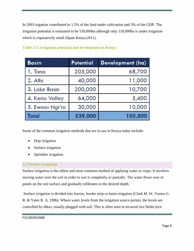
In 2003 irigation contributed to 1.5% of the land under cultivation and 3% of the GDP. The
irrigation potential is estimated to be 539,000ha although only 110,000ha is under irrigation
which is coparatively small (Spate Kenya,2011).
Table 2-1: Irrigation potential and development in Kenya
Some of the common irrigation methods that are in use in Kenya today include:
Drip irrigation
Surface irrigation
Sprinkler irrigation
2.2 Surface irrigation
Surface irrigation is the oldest and most common method of applying water to crops. It involves
moving water over the soil in order to wet it completely or partially. The water flows over or
ponds on the soil surface and gradually infiltrates to the desired depth.
Surface irrigation is divided into furrow, border strip or basin irrigation (Clark M. W, Varma G.
R, & Yates R. A, 1986). Where water levels from the irrigation source permit, the levels are
controlled by dikes, usually plugged with soil. This is often seen in terraced rice fields (rice
F21/0039/2008
Page 7
paddies) for example small-scale farmers managed irrigation systems in the dry zone lowland
agro-ecological zone of Sri Lanka (Rekha N. & Jayakumara M. A, 2010). Surface irrigation
methods are best suited to soils with low to moderate infiltration capacities and to lands with
relatively uniform terrain with slopes less than 2-3%.
2.3 Components of a surface irrigation system
Surface irrigation system consists of the following components:
2.3.1 The water source
The source of water can be surface water or groundwater. Water can be abstracted from a river,
lake, reservoir, borehole, well, spring, etc. In this project the source of water is Tana River.
2.3.2 The intake facilities
The intake is the point where the water enters into the conveyance system of the irrigation area.
Water may reach this point by gravity or through pumping. For this project, the intake facility
will be located downstream Kindaruma dam.
2.3.3 The conveyance system
Water can be conveyed from the Head works to the inlet of a night storage reservoir or a block of
fields either by gravity, through open canals or pipes, or through pumping into pipelines. The
method of conveyance depends mostly on the terrain (topography and soil type) and on the
difference in elevation between the intake at the headwork and the irrigation scheme. In order to
be able to command the intended area, the conveyance system should discharge its water at the
highest point of the scheme. The water level in the conveyance canal itself does not need to be
above ground level all along the canal, but its starting bed level should be such that there is a
sufficient command for the lower order canals. Where possible, it could run quasi parallel to the
contour line.
2.3.4 The field canal and/or pipe system
Canals or pipelines are needed to carry the water from the conveyance canal or the NSR to a
block of fields. They are called the main canal or pipeline. Secondary canals or pipelines supply
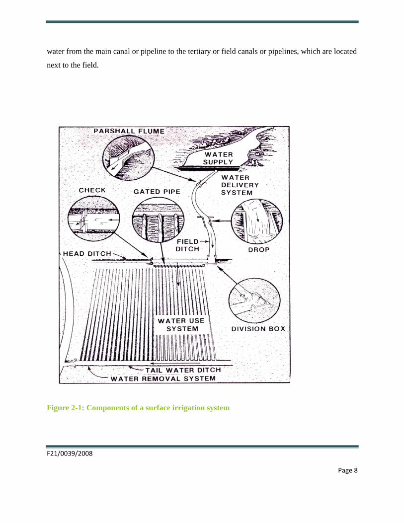
F21/0039/2008
Page 8
water from the main canal or pipeline to the tertiary or field canals or pipelines, which are located
next to the field.
Figure 2-1: Components of a surface irrigation system
F21/0039/2008
Page 9
2.3.5 The infield water use system
This refers mainly to the method of water applied to the field, which can be furrow, border strip
or basin irrigation. In irrigation system design, the starting point is the infield water use system as
this provides information on the surface irrigation method to use, the amount of water to be
applied to the field and how often it has to be applied.
2.3.6 The drainage system
This is the system that removes excess water from the irrigated lands. The water level in the
drains should be below the field level and hence field drains should be constructed at the lower
end of each field. These fields or tertiary drain would then be connected to secondary drains and
then the main drain, from where excess water is removed from the irrigation scheme.
2.3.7 Accessibility infrastructure
The farms are to be made accessible through the construction of main roads leading to the farm
roads within the field.
2.4 Design of Scheme Layout
The general layout of the surface irrigation system is guided by the topography of the land among
other factors. The layout must be designed in such a way that the whole system area is being
commanded and also the excess water is drained safely from the scheme. The access to the area
must also be ensured in such a way that farmers will not have to carry their produce for a long
distance on their backs before accessing the points where vehicles or animal carts can pick them
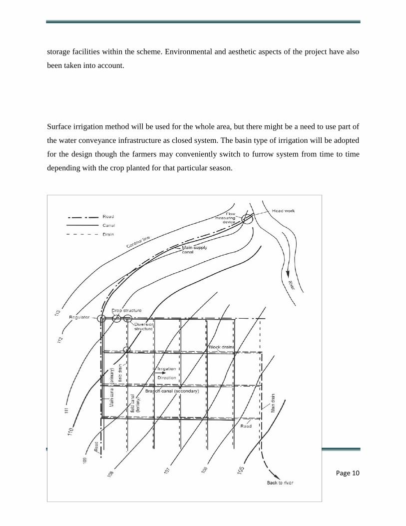
for transportation. Figure 1-2 shows an example of Typical Scheme Layout.
The Layout Design takes into account the above considerations in order to come up with an
optimal layout which also recognizes the need for social, educational, recreational, health and
F21/0039/2008
Page 10
storage facilities within the scheme. Environmental and aesthetic aspects of the project have also
been taken into account.
Surface irrigation method will be used for the whole area, but there might be a need to use part of
the water conveyance infrastructure as closed system. The basin type of irrigation will be adopted
for the design though the farmers may conveniently switch to furrow system from time to time
depending with the crop planted for that particular season.
F21/0039/2008
Page 11
Figure 2-2: Typical layout of a surface irrigation scheme on a uniform flat topography
2.5 Crop Water Requirement
The system water requirement is the total amount of water that will be supplied for effective
scheduled irrigation. The following primary assumptions have been made in the determination of
the scheme water requirements:
The potential Evapotranspiration is maximum
The irrigated area is 100% of the effective irrigation area of the scheme as agreed by the
members
The crop is at its peak growth
The amount of soil water storage is negligible
The following factors / parameters are considered during the review of the general water
requirements:
Crops and cropping patterns;
Crop factors (Kc);
Evapotranspiration and effective rainfall;
Irrigation efficiencies (for sprinkler irrigation system);
Irrigation hours per day and no. of settings per day;
F21/0039/2008
Page 12
Irrigation days per week;
Irrigation area.
ETcrop =ETo x Kc;
Where;
ETo =Evapo-transpiration, which is given by; Evaporation from free water surface x adjustment
factor (0.75 for highlands above 1100 m.a.s.l and 0.8 for hot and dry low areas below 1100
m.a.s.l)
Kc - Crop Coefficient taken as 0.9 for most of the crops.
Various crops have been proposed to be produced under irrigation, which include:
Beans
Cabbage
Sweet pepper
Tomatoes
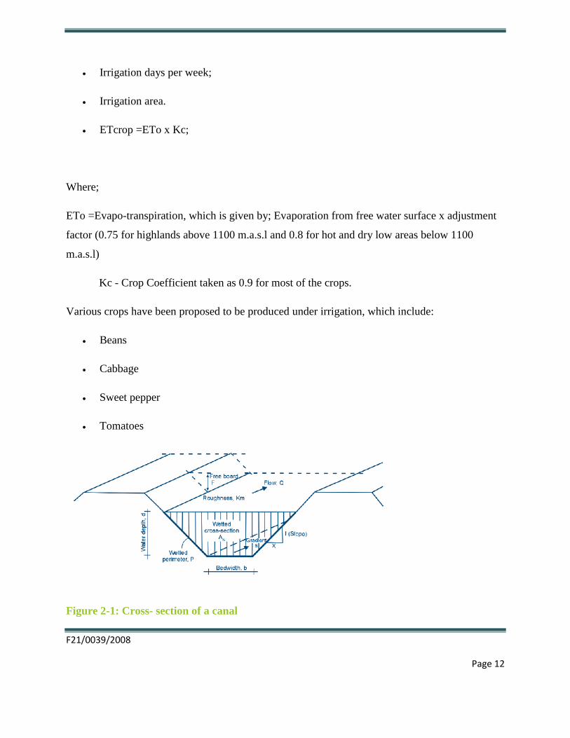
Figure 2-1: Cross- section of a canal

F21/0039/2008
Page 13
Chapter 3
3.0 THEORETICAL FRAMEWORK
3.1 Penman-Monteith equation
In 1948, Penman combined the energy balance with the mass transfer method and derived an
equation to compute the evaporation from an open water surface from standard climatological
records of sunshine, temperature, humidity and wind speed. This so-called combination Crop
evapo-transpiration method was further developed by many researchers and extended to cropped
surfaces by introducing resistance factors. The equation is as follows
ETo = [0.408 ∆ (Rn-G) + γ900 / (T+273) x U2 (es-ea)]/ [∆+ γ (1+0.34U2)]
Equation 3-1: Penman-Monteith equation
Where
ETo- reference evapo-transpiration [mm day-1],
Rn -net radiation at the crop surface [MJ m-2 day-1],
G- Soil heat flux density [MJ m-2 day-1],
T- Air temperature at 2 m height [°C],
u2 -wind speed at 2 m height [ms-1],
es - Saturation vapour pressure [kPa],
ea - actual vapour pressure [kPa],
es-ea - saturation vapour pressure deficit [kPa],
Δ -slope vapor pressure curve [kPa °C-1],
F21/0039/2008
Page 14
γ – Psychrometric constant [kPa °C-1].
3.2 Crop coefficient approach
In the crop coefficient approach the crop evapotranspiration, ETc, was calculated by multiplying
the reference crop evapotranspiration, ETo, by a crop coefficient, Kc:
ETc = Kc ETo
Equation 3-2: crop evapo-transpiration
Where ETc- crop evapo-transpiration [mm d-1],
Kc- crop coefficient [dimensionless],
ETo- reference crop evapotranspiration [mm d-1].
Most of the effects of the various weather conditions are incorporated into the ETo estimate.
Therefore, as ETo represents an index of climatic demand, Kc varies predominately with the
specific crop characteristics and only to a limited extent with climate. This enables the transfer of
standard values for Kc between locations and between climates. This has been a primary reason
for the global acceptance and usefulness of the crop coefficient approach and the Kc factors
developed in past studies.
3.3 Crop factor (Kc)
The respective values of crop factor (Kc) for the different crops and growth stages was based on
four stages of growth i.e. initial stage, crop development stage, mid-season stage and late season
stage.
F21/0039/2008
Page 15
3.4 Net Irrigation Requirement (NIR)
The NIR will be calculated using formula as follows:
NIR= ETCrop - Pe, + (SAT + PERC + WL)
Equation 3-3: NIR
Where; ETCrop = Crop Water Requirement [mm/day];
Pe = Effective rainfall [mm/day]
SAT = Water required for pudding [200 mm/day];
PERC = Percolation and seepage losses [0.1 mm/day];
WL = Water layer depth [100 mm/day];
SAT, PERC and WL values are only applicable to paddy rice farming. Upland and horticulture
crops do not require water for saturation, percolation and maintenance of the water layer above
the soil. Hence, these values were assumed to be zero.
3.5 Gross Irrigation Requirement, GIR
The GIR was calculated using formula as follows,
GIR = NIR / (overall irrigation efficiency, Eo).
Equation 3-4: GIR
Where; Eeff = Ec x Ed x Ea
Ec= Conveyance efficiency;
Ed = Distribution efficiency;
Ea= Application efficiency;

F21/0039/2008
Page 16
The adopted irrigation efficiencies as recommended by FAO Irrigation and Drainage Paper No.24
were:
Conveyance = 95% (partially lined canals) and 90% (earth canals);
Distribution = 90% (earth canals);
Application = 65%
3.6 Project Water Requirement (PWR)
The PWR was based on a 24-hour irrigation duration using the following equation:
PWR= GIR x A
Equation 3-5: Project water requirement
Where; A= Net irrigation area
3.7 Design command area
The required canal discharge depends on the field area to be irrigated (known as the 'command
area'), and the water losses from the canal. For a design command area A (m2), the design
discharge required Q (l/s) for irrigation hours (H) every day, was given by the field-irrigation
requirement multiplied by the area, divided by the time (in seconds):
Q = If * A
H*60*60 plus canal losses
Equation 3-6: Design Discharge required
3.8 Canal Design
The general steps involved in the design of the canal networks include:
Performing hydrologic computations and select design flows
Estimation of soil erodibility
Defining the type of channel lining material desired
F21/0039/2008
Page 17
Defining the channel slope and any restrictions on channel geometry
Determination of maximum permissible depth of flow, or maximum permissible
velocity of flow for lining material
Selection of channel geometry and channel lining suitable for the design flows being
considered
Consideration of other possible factors.
The project canal network was designed to convey water throughout the area. In order to ensure
effective water distribution, consideration was put on the general topography of the project so as
to minimize pressure head loss much needed at crop point.
The canal network consisted of the following:
Conveyance
Main Line
Sub Main lines
Feeder Lines
Other canal appurtenances.
Manning’s equation of flow was used to calculate dimensions of the canals.
Q = AV
Also
Q = Km × A × R2/3
× S1/2
Equation 3-7: Manning’s
Where
Q = Flow Rate (m3/s)
F21/0039/2008
Page 18
Km = Manning’s roughness coefficient = 1/n
A = Canal cross section Area (m2) = bd + Zd
2
S = Slope (m/m)
V = Velocity (m/s)
R = Hydraulic Radius (m)
P = b + 2d (1 + Z2)1/2
Equation 3-8: Wetted perimeter
Where;
b = bed width (m)
d = water depth (m)
Z = canal side slopes (m/m)
R = A /P =
⁄
Equation 3-9: Hydraulic radius
Froude number is given by the equation below;
Fr =
Equation 3-10: Froude no.
Where;
F21/0039/2008
Page 19
u = Flow velocity in the canal (m/s)
g = Gravitational force (9.81 m/s2)
Z = Depth of flow (m)
For the wave to be stationary (critical), Fr = 1
However, for open channels;
If Fr > 1, the flow is super-critical, rapid or shooting and is characterized by shallow and
fast fluid motion.
If Fr < 1, the flow is sub-critical, tranquil or streaming and is characterized by relative to
supercritical flow this is slow and deep fluid motion.
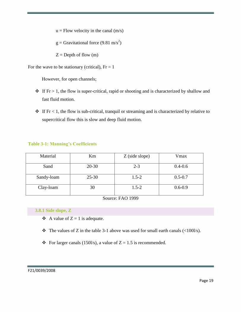
Table 3-1: Manning’s Coefficients
Material Km Z (side slope) Vmax
Sand 20-30 2-3 0.4-0.6
Sandy-loam 25-30 1.5-2 0.5-0.7
Clay-loam 30 1.5-2 0.6-0.9
Source: FAO 1999
3.8.1 Side slope, Z
A value of Z = 1 is adequate.
The values of Z in the table 3-1 above was used for small earth canals (<100l/s).
For larger canals (150l/s), a value of Z = 1.5 is recommended.
F21/0039/2008
Page 20
3.8.2 Velocity, V
The maximum velocities were best chosen at lower end of the given range. Minimum velocity
should be in the order of 0.15 m/sec to avoid silting up of the supply canal and main feeders.
3.8.3 The water depth, b and bed width, d ratio
The recommended range of the ratio is 0.4-1.0. A minimum b of 0.30m is used and increased
only in multiples of 0.10.
Table 1-2: Recommended Values of d/b ratios
Water depth d/b ratio
Small (d<0.75m) 1 (clay) – 0.5 (sand)
Medium (d = 0.75 –
1.50m)
0.5 (clay) – 0.33 (sand)
Large (d>1.50m) <0.33
3.8.4 Freeboard
The freeboard acts as a safety against overflow of the canal due to a water depth higher than the
calculated design depth.
The freeboard of earth irrigation canals is in general about 0.2 – 0.3 times the depth of flow. A
minimum value of about 0.10 is recommended. The freeboard is adjusted to obtain values of the
canal depth (water depth + freeboard) which are multiples of 0.05m.
Pipeline Flow Hydraulics
The flow hydraulics in the pipe system was used to determine the following:
The friction head losses along the pipeline

F21/0039/2008
Page 21
The variation in pressures along the pipeline.
The Hazen-Williams equation was used in determination of friction head losses within the pipe
system i.e.
Hf = 6.843*L*(V/C) ^1.852/ (D^1.167)
Equation 3-11: Hazen- Williams
Where;
Hf =friction head losses (m)
L =Length of flow (m)
V =Average flow velocity (m2)
D =Diameter of the pipe m)
C =Roughness coefficient taken as 140 for uPVC and 125/115 for GI pipes.
The pressure variations along the pipe line was determined as follows:
The Static Head (Hs) =The Total Head at a point in the canal line;
The Energy Grade Line (EGL)=Static Head (Hs) – Friction Losses (Hf);
The Hydraulic Grade line(HGL)= EGL – Velocity head (Hv);
The Operating Pressure Head (HP) =HGL – Pipe Invert Level (PIL).
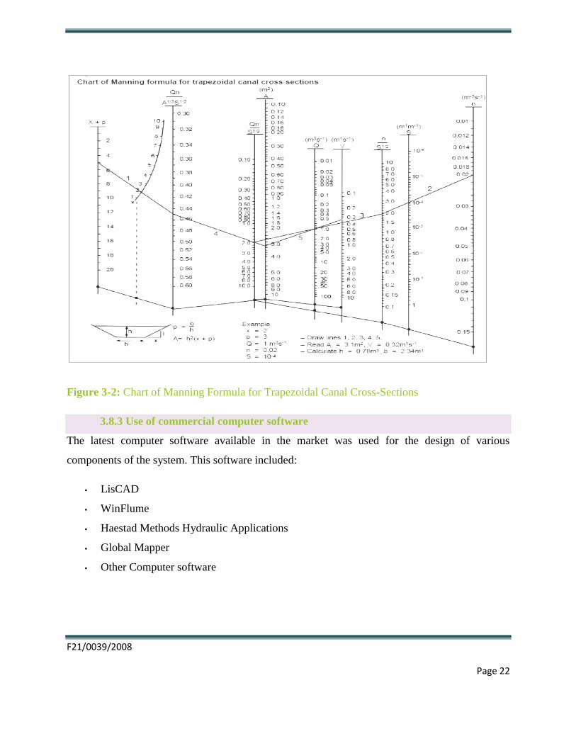
3.8.1 Use of Manning Formula Charts
The chart was useful in the hydraulic design of canals networks through trial and error. Figure 3-
2 below presents the chart used to determine optimum canal parameters for trapezoidal canal
sections.
F21/0039/2008
Page 22
Figure 3-2: Chart of Manning Formula for Trapezoidal Canal Cross-Sections
3.8.3 Use of commercial computer software
The latest computer software available in the market was used for the design of various
components of the system. This software included:
• LisCAD
• WinFlume
• Haestad Methods Hydraulic Applications
• Global Mapper
• Other Computer software
F21/0039/2008
Page 23
Chapter 4
4.0 METHODOLOGY
4.1 The area of study
The project is in Thaana nzau location of the lower Tana. All the data was obtained from the area
except those obtained from different departments or firms such as Metrological department
(Gawaher M. & Amin M. S, 2005).
4.2 Estimation of crop water requirements
CLIMWAT and CROPWAT are the software that was used to estimate the crop water
requirement.
The choice of crops to be grown under irrigation in the project area was based on;
a. Which crop has high return
b. Suitability of soil to grow the selected crop
c. Agro-climatic conditions
d. Topography
e. Growth cycle of the crop
Water requirements will be determined based on the following:
Selected crops and cropping patterns which will be determined using questionnaires/
interviews
Reference Evapo-transpiration (ETo);
Crop factor (kc);
Effective rainfall from nearby metrological department
F21/0039/2008
Page 24
Additional water requirements, in particular for paddy;
Irrigation efficiencies (conveyance, distribution and application);
Irrigation schedule (24-hour duration and on a daily basis);
Area to be irrigated
This was calculated using FAO 56 crop water requirements standards. The FAO Penman-
Monteith method is maintained as the sole standard method for the computation of ETo from
meteorological data. According to the formula
ETo = [0.408∆(Rn-G)+ γ900/(T+273)xU2(es-ea)]/ [∆+γ(1+0.34U2) ]
4.2.1 CROPWAT procedure:
The ETo data was loaded
The rainfall data was also loaded and the effective rainfall was automatically calculated
The soil data for the area was then specified
The crop was the selected then the date of planting was also chosen
The next tab of CROPWAT calculated the crop water requirement
Crop factor (Kc)
The respective values of crop factor (Kc) for the different crops and growth stages was based on
four stages of growth i.e. initial stage, crop development stage, mid-season stage and late season
stage. This value was selected from the Kenyan Atlas and CROPWAT analysis.
4.2.2 Net Irrigation Requirement (NIR)
The NIR was calculated using equation 3-3 and the crop demand obtained from CROPWAT
(IlyamukuruL P. A. & Iyamuremye J. D., 2011):
F21/0039/2008
Page 25
4.3. Canal design
4.3.1 Determination of system layout
The elevation and height of the field was obtained using the GPS. This helped in getting the
coordinates and the tracks and further getting the system layout.
Layout Procedure
Acquisition cadastral map of the area
The above map was digitize in AutoCAD(in cad, insert – raster image – digitize)
The pieces of the cadastral map were joined to make a whole map in AutoCAD,
for example a main road was used to join it.
The topographical map of the area was then Geo referenced
A major feature in the topographical map, i.e. road, river or shopping center was
identified
The same feature was also identified in the cadastral map
The cadastral map was moved to the topographical map with identified feature as
the base point
Scaled the moved cadastral map to fit the topographical map
Using boundaries/ roads/ contour lines, the canal paths were finally drawn.
4.3.2 Profile Generation
The Global Mapper was used to generate the canal profiles. The following steps were followed:
Opened my own data
The Kenyan DEM was loaded
In the file menu, selected open data files
Then the drawn layout of the area was opened
Projection selected as UTM
Thaana Nzau zone -37
Datum ACR 1960
Select generate profile path command
Using the command follow the canals then right click at the end

F21/0039/2008
Page 26
The profiles are generated as shown in Figure 4-1 below
then specified the spacing of the chainage values
Saved as CSV file as shown in Figure 4-2 below
Figure 4-1: Profile generation using Global Mapper
F21/0039/2008
Page 27
4.3.3 Iteration Method using Spreadsheet
This involved the use of Excel program to perform iterations that gave the accurate calculations
for Canal design. Figure 4-2 shows the Excel program for performing the Canal design.
Figure 4-2: Canal Design by Use of Excel Application
F21/0039/2008
Page 28
Figure 4-3: Flow Chart of Canal Design Calculations
The discharge of each canal was determined from net irrigation requirement while Km, x and S
was read from Manning’s design tables for sandy-loam soil type. Roughness coefficient normally
depends on the type and condition of channel sides and bottoms. In the Irrigation project the
channels will be earthen and partly lined (concrete/stone pitching) depending on different
conditions.
The design involved use of computer software which has been assembled to perform certain
specific purposes. The Auto Lisps routines of AutoCAD were used for hydraulic design of canal
and drop structures. The results from these routines have been tested against those obtained from
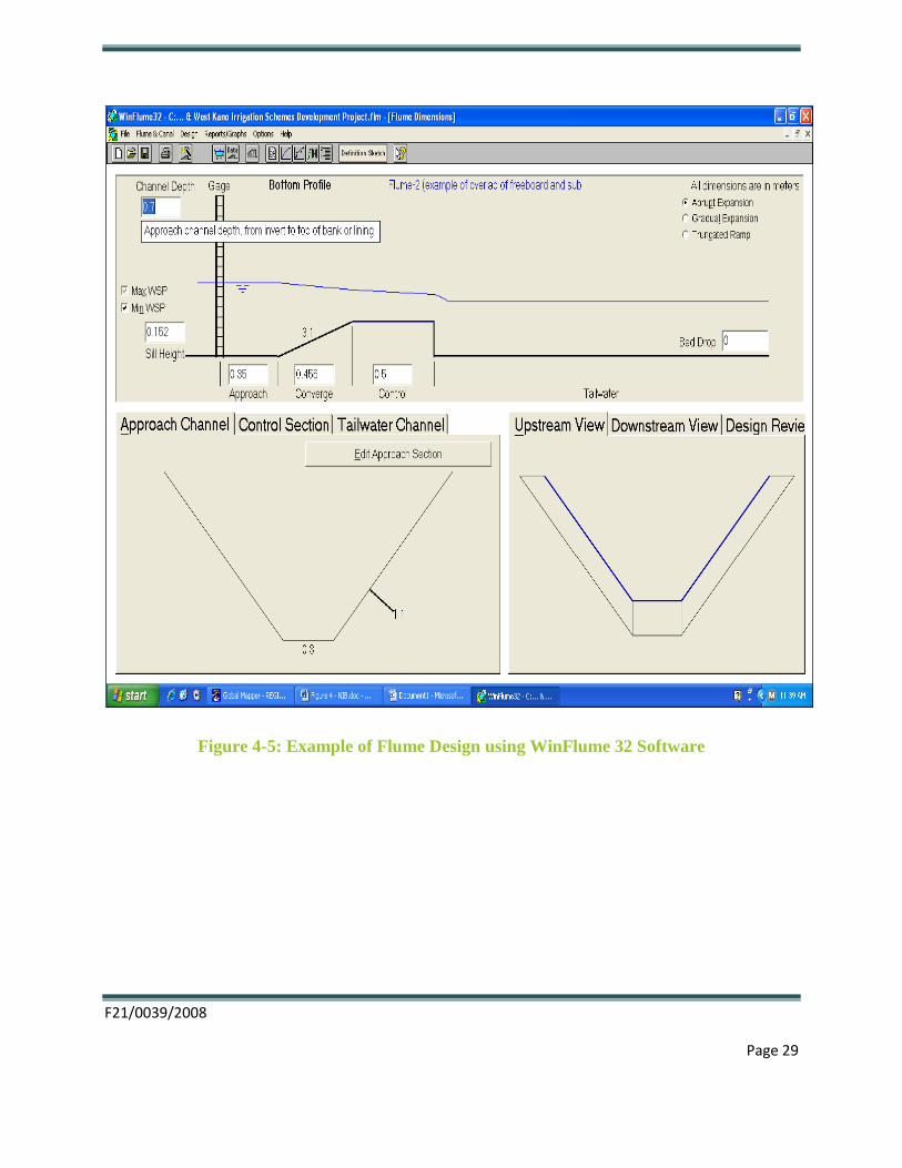
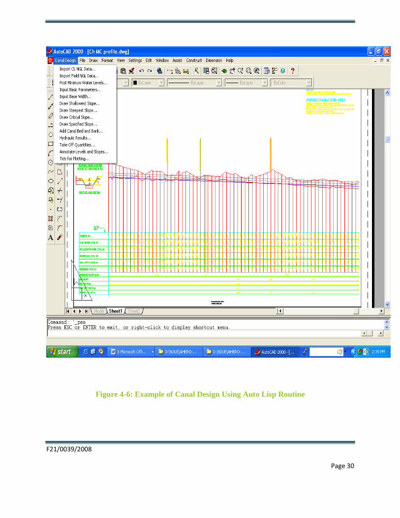
basic calculations using the design equations and found to be accurate. Figure 4-5 below shows
flume design using Win Flume 32 and figure 4-6 shows the canal profile designed from an Auto
Lisp routine.
F21/0039/2008
Page 29
Figure 4-5: Example of Flume Design using WinFlume 32 Software
F21/0039/2008
Page 30
Figure 4-6: Example of Canal Design Using Auto Lisp Routine
F21/0039/2008
Page 31
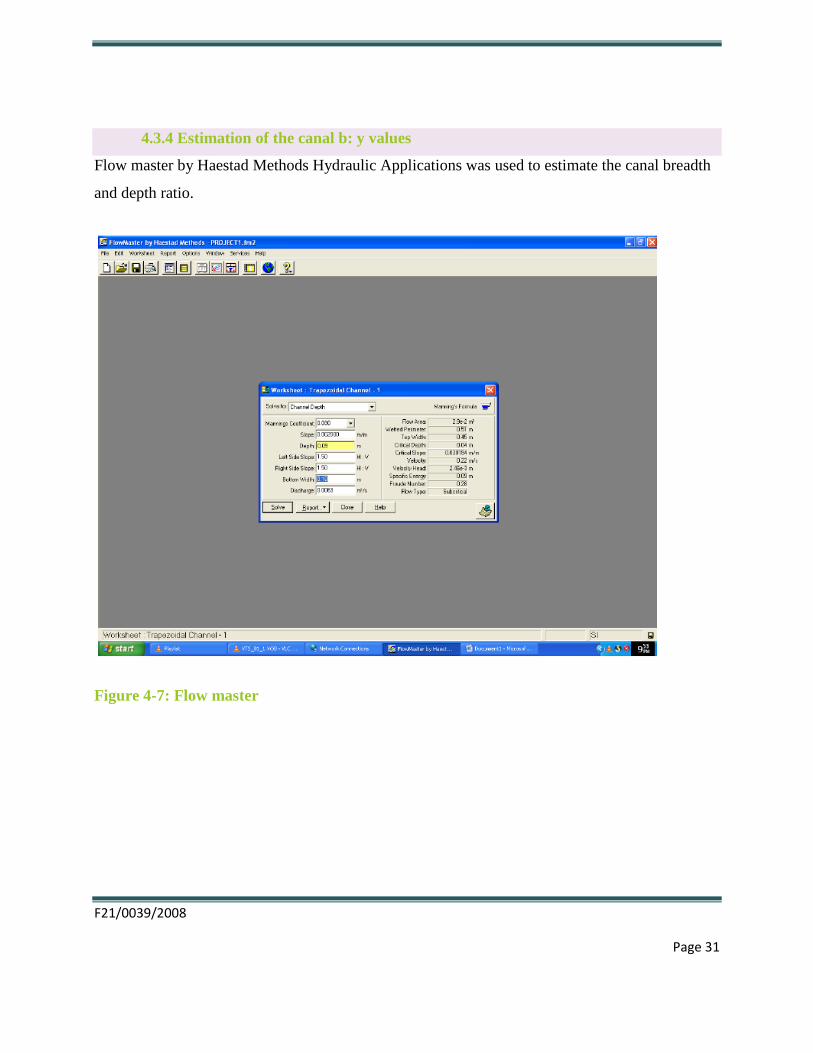
4.3.4 Estimation of the canal b: y values
Flow master by Haestad Methods Hydraulic Applications was used to estimate the canal breadth
and depth ratio.
Figure 4-7: Flow master

F21/0039/2008
Page 32
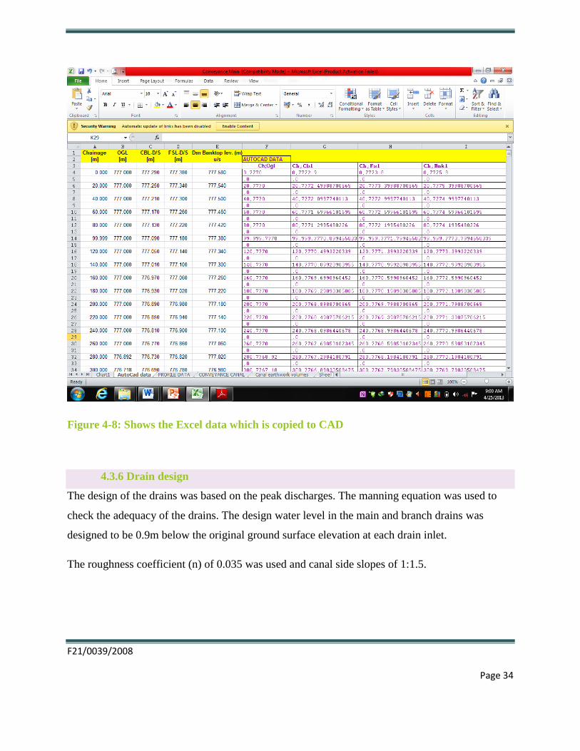
4.3.5 Profile generation in cad
- Rename the given template
- Delete one of the existing template profile
- Type PL in tab command
- Open the AutoCAD data in excel sheet
- Copy the first column of CBL to CAD as shown from Figure 4-8
- Also copy and paste the second column of the CBL
- Type APPLOAD in CAD command – joinlisp – load – close
- Type PQUA – enter – Datum fo this file
o Select the least OGL ie 899-20
o Type 1:2000 – Horizontal scale
o Type 1:200 – Vertical scale
o Select polyline
i. Pipe invert – top line of generated profile
ii. Ground level – Bottom line
- Type PANNOT in the new window developed
Pipe=0
Lining = 0
Bedding 100 – close
- Open new AutoCAD window (Cntrl+ N)
- Delete the ISO Ao file opened
- In the excel select the third column (ch FSL) then paste in Cad
- Select fourth BKL column then paste in Cad

F21/0039/2008
Page 33
- Type APPLOAD – joinlisp – load – close
- Copy with base point(choose that in excel)
- In cad command type 0,0 enter
- Paste with original coordinates
- Select upto ground level from below (in cad)
- Ensure OSNAP is on
- Move 2 steps down of invert row
- The last 2 (3rd
and 4th
columns) are married to the first two columns
- Select (ground invert level) of the last two.
- Copy and paste
- Offset by 20 to create a line
- Select first line then extend
- Remove and delete rows
Finally, marry and match the properties to get the profile. Clean then set the profiles as shown in
Figure 4-6 above.
F21/0039/2008
Page 34
Figure 4-8: Shows the Excel data which is copied to CAD
4.3.6 Drain design
The design of the drains was based on the peak discharges. The manning equation was used to
check the adequacy of the drains. The design water level in the main and branch drains was
designed to be 0.9m below the original ground surface elevation at each drain inlet.
The roughness coefficient (n) of 0.035 was used and canal side slopes of 1:1.5.
F21/0039/2008
Page 35
4.3.6 Hydraulic structures
Conveyance structures:
These are structures that are necessary to let the conveyance (passage) of irrigation water
smoothly.
Drop Structures:
Drop structures are flow conveyance structures that are installed in canals when the natural land
slope is too steep compared to the design canal gradient to convey water down steep slopes
without erosion. The structure should be able to allow safe flow of the canal discharge and be
within the maximum permissible level of fluctuations upstream. For larger drops chutes are used.
Drops are used to:
Control upstream water velocity to reduce erosion;
Drop the water to a lower level;
Dissipate the excess energy created by the drop;
Control downstream erosion.
4.3.7 Culverts
The actual road width was considered for design purposes. Roads were designed with the
following taken into consideration during checking and designing processes.
Allowable head losses
Road elevation in case of road crossing;
Water silt load
Expected load was designed using the following general design criteria:
A minimum diameter of 0.46mm was used to avoid clogging;

F21/0039/2008
Page 36
Inlet and outlet transitions of 3 x diameter of the pipe or culvert box with a minimum of 2
metres;
A flow velocity within the range of 1 - 1.5m/s;
Protection at the transitions
Allowance for hydraulic losses as follows:
- Culvert length less or equal to 8 metres total head loss (H) =2 x V2/2g;
- Culvert length greater than 8 metres: head loss (H) = 3 x V2/2g .
Provide a 0.15m concrete encasement for culverts with cover of less than 0.9m (at least
0.50m total cover).
4.3.8 Regulation structures
Division boxes:
In the design and analysis of the division structures the following aspects were considered:
The possibility of the structure serving dual purpose;
Some flexibility in water distribution since a rotational water distribution system is
envisaged;
Use of drain pipes as far as possible for self cleaning purposes;
The amount of head available for the division structure to command the flow;
Back water effect upstream of the structure to avoid submerging other structures or
overtopping of the canal;
Protection of the structure against scouring due to changes in flow condition.
F21/0039/2008
Page 37
The weir coefficient of 1.6 for normal rectangular short crested weirs was adopted.
The minimum dimensions of the structure will depend on its performance in the fully open
position. The width of the outlet was proportional to the division of water flow to be made. The
walls are made of concrete.
Turnouts:
The turnouts was assessed for adequacy to carry adequate discharge as per the demand of the
canal in relation to the water level at the location of the turnout/off-take.
The turnouts consists of Inlet from the main canal, slide gates, pipe culverts /open channel and
out let transition to branch canal. The structure design took into consideration the shape of
turnout opening (orifice / open channel).
Checks:
In this assignment, the check structures will be designed to function as overflow weirs, orifices or
a combination of both. In cases where structures are combined it will be ensured that it meets all
the purposes.
Cross drainage:
Culverts will be used to safely convey drainage water upstream of major canals. In cases where
cross drainage is required, the use of culverts will be maintained
Canal lining:
Although unlined canals are the most common worldwide due to their cheap construction cost,
sections of canals in the project was lined so as to increase the conveyance efficiency and thus
make more water available. Canal lining also reduces seepage, weed growth and substantially
reduces canal maintenance.
The material recommended for lining is concrete due to its durability and the availability of
materials (cement, fine and coarse aggregates). If properly constructed and maintained, concrete
canals can have a serviceable life of over 40 years.
F21/0039/2008
Page 38
Flood protection dykes:
The design of the flood protection dykes was based on the need to ensure that the seepage
gradient (hydraulic grade line) falls within the body of the dyke. The recommended section
parameters for a flood protection dyke of up to 3.25 m are as follows:
Top width : 2.5 – 3.5 m
River side slope : 2:1 to 5:1 (Horizontal to Vertical)
Land side slope : 2:1 to 7:1 (Horizontal to Vertical)
Freeboard : 0.3 – 1.5 m above the high flood level;
Hydraulic grade line : at least 1.0 m below the top surface of the embankment
Measuring structures
Flow measurement in canals entails introducing a calibrated structure that partially restricts the
flow of water and provides for a free fall to ensure that upstream and downstream flows are
independent.
4.3.9 Other structures
Watering steps:
The community will be using the canal water for domestic purposes. To reduce the canal
damages, watering steps will be constructed. The watering steps will be standardized as much as
possible.
General design considerations included the following:
The population likely to use the structure to establish the width and numbers;
The safety of the user during water fetching for sizing of the steps;
Protections against erosion
F21/0039/2008
Page 39
Animals watering points:
Canal damage is mostly due to uncontrolled animal movement and watering points. To reduce the
damages resulting from this, provision of animal watering points will be done at appropriate
locations along the canal networks.
Design considerations included:
Location which depend on availability of the land (space) and accessibility;
Size of the basin depending on the animal population;
Protection against erosion.
Standard design for the animal watering taking into consideration of the above aspects was
provided

F21/0039/2008
Page 40
Chapter 4
5.0 RESULTS AND DISCUSSION
Gross location potential 20Ha
Net irrigable area 10Ha
Number of beneficiaries 20 farmers
Irrigation plot size 0.55Ha
5.1 Crop Water Requirement
Though there is a cropping pattern agreed upon by the farmers and the District Horticultural
Officer, it is highly unlikely, as already is the case in similar irrigation schemes in the region, that
there will be a fixed irrigation pattern on which water requirements can be based at any one time
during the year.
Consequently, the use of an average crop factor, Kc, of 0.9 as is common practice under such
circumstances.
5.1.1 Reference Crop Evapotranspiration, ETo
Mwingi Meteorological Station has been used since it is close to and representative of the project
area. The data from the station has also been compared, analyzed and published data by T
Woodhead (1968) with respect to the evapotranspiration, ETo. These two sets of data agree well
with each other and therefore the data can confidently be used to compute the crop water
requirement. (Source-Mwingi Agriculture weather station)
F21/0039/2008
Page 41
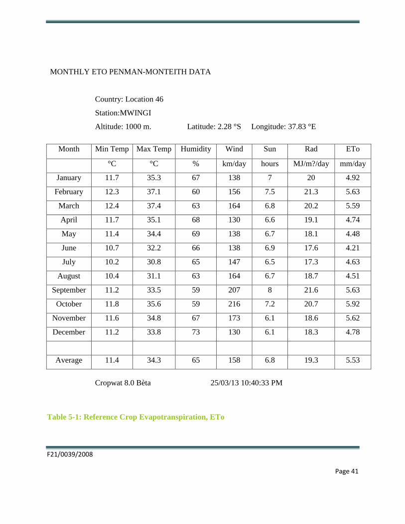
MONTHLY ETO PENMAN-MONTEITH DATA
Country: Location 46
Station:MWINGI
Altitude: 1000 m. Latitude: 2.28 °S Longitude: 37.83 °E
Month Min Temp Max Temp Humidity Wind Sun Rad ETo
°C °C % km/day hours MJ/m?/day mm/day
January 11.7 35.3 67 138 7 20 4.92
February 12.3 37.1 60 156 7.5 21.3 5.63
March 12.4 37.4 63 164 6.8 20.2 5.59
April 11.7 35.1 68 130 6.6 19.1 4.74
May 11.4 34.4 69 138 6.7 18.1 4.48
June 10.7 32.2 66 138 6.9 17.6 4.21
July 10.2 30.8 65 147 6.5 17.3 4.63
August 10.4 31.1 63 164 6.7 18.7 4.51
September 11.2 33.5 59 207 8 21.6 5.63
October 11.8 35.6 59 216 7.2 20.7 5.92
November 11.6 34.8 67 173 6.1 18.6 5.62
December 11.2 33.8 73 130 6.1 18.3 4.78
Average 11.4 34.3 65 158 6.8 19.3 5.53
Cropwat 8.0 Bèta 25/03/13 10:40:33 PM
Table 5-1: Reference Crop Evapotranspiration, ETo

F21/0039/2008
Page 42
The ETo for the driest months of August/September and January/February before the on-set of
the rains has been employed. The average monthly evapotranspiration for these months range
from 126.3 – 154.5 with an average of 140.4 mm (or 4.93 mm/day).
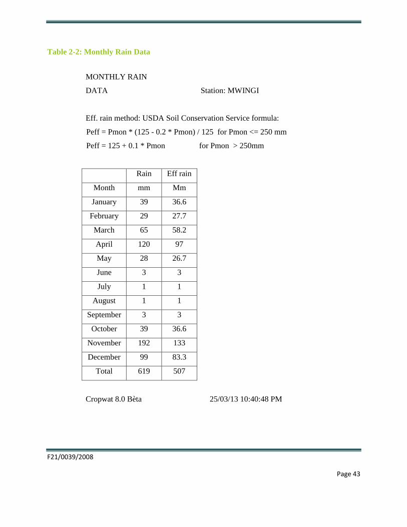
The effective rainfall for the project has been calculated for each month using the rainfall data
from Mwingi Meteorological Station and presented in Table above. From the table, the effective
rainfall for the months of January, February, August and September are given as 36.6, 27.7, 1.0
and 3.0 mm respectively. The highest effective rainfall is found to be 133.0 mm in the month of
November while the lowest is 1.0mm occurring in July and August.
F21/0039/2008
Page 43
Table 2-2: Monthly Rain Data
MONTHLY RAIN
DATA
Station: MWINGI
Eff. rain method: USDA Soil Conservation Service formula:
Peff = Pmon * (125 - 0.2 * Pmon) / 125 for Pmon <= 250 mm
Peff = 125 + 0.1 * Pmon for Pmon > 250mm
Rain Eff rain
Month mm Mm
January 39 36.6
February 29 27.7
March 65 58.2
April 120 97
May 28 26.7
June 3 3
July 1 1
August 1 1
September 3 3
October 39 36.6
November 192 133
December 99 83.3
Total 619 507
Cropwat 8.0 Bèta 25/03/13 10:40:48 PM
F21/0039/2008
Page 44
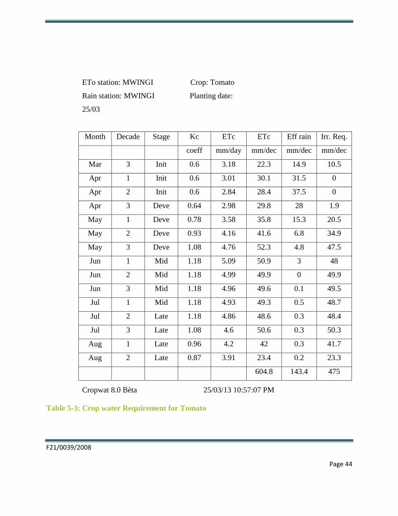
ETo station: MWINGI Crop: Tomato
Rain station: MWINGI Planting date:
25/03
Month Decade Stage Kc ETc ETc Eff rain Irr. Req.
coeff mm/day mm/dec mm/dec mm/dec
Mar 3 Init 0.6 3.18 22.3 14.9 10.5
Apr 1 Init 0.6 3.01 30.1 31.5 0
Apr 2 Init 0.6 2.84 28.4 37.5 0
Apr 3 Deve 0.64 2.98 29.8 28 1.9
May 1 Deve 0.78 3.58 35.8 15.3 20.5
May 2 Deve 0.93 4.16 41.6 6.8 34.9
May 3 Deve 1.08 4.76 52.3 4.8 47.5
Jun 1 Mid 1.18 5.09 50.9 3 48
Jun 2 Mid 1.18 4.99 49.9 0 49.9
Jun 3 Mid 1.18 4.96 49.6 0.1 49.5
Jul 1 Mid 1.18 4.93 49.3 0.5 48.7
Jul 2 Late 1.18 4.86 48.6 0.3 48.4
Jul 3 Late 1.08 4.6 50.6 0.3 50.3
Aug 1 Late 0.96 4.2 42 0.3 41.7
Aug 2 Late 0.87 3.91 23.4 0.2 23.3
604.8 143.4 475
Cropwat 8.0 Bèta 25/03/13 10:57:07 PM
Table 5-3: Crop water Requirement for Tomato
F21/0039/2008
Page 45
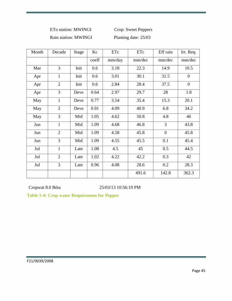
ETo station: MWINGI Crop: Sweet Peppers
Rain station: MWINGI Planting date: 25/03
Month Decade Stage Kc ETc ETc Eff rain Irr. Req.
coeff mm/day mm/dec mm/dec mm/dec
Mar 3 Init 0.6 3.18 22.3 14.9 10.5
Apr 1 Init 0.6 3.01 30.1 31.5 0
Apr 2 Init 0.6 2.84 28.4 37.5 0
Apr 3 Deve 0.64 2.97 29.7 28 1.8
May 1 Deve 0.77 3.54 35.4 15.3 20.1
May 2 Deve 0.91 4.09 40.9 6.8 34.2
May 3 Mid 1.05 4.62 50.8 4.8 46
Jun 1 Mid 1.09 4.68 46.8 3 43.8
Jun 2 Mid 1.09 4.58 45.8 0 45.8
Jun 3 Mid 1.09 4.55 45.5 0.1 45.4
Jul 1 Late 1.08 4.5 45 0.5 44.5
Jul 2 Late 1.02 4.22 42.2 0.3 42
Jul 3 Late 0.96 4.08 28.6 0.2 28.3
491.6 142.8 362.3
Cropwat 8.0 Bèta 25/03/13 10:56:19 PM
Table 5-4: Crop water Requirement for Pepper
F21/0039/2008
Page 46
Month Decade Stage Kc ETc ETc Eff rain
Irr.
Req.
coeff mm/day mm/dec mm/dec mm/dec
Mar 3 Init 0.5 2.65 18.6 14.9 6.8
Apr 1 Init 0.5 2.51 25.1 31.5 0
Apr 2 Init 0.5 2.37 23.7 37.5 0
Apr 3 Init 0.5 2.33 23.3 28 0
May 1 Init 0.5 2.28 22.8 15.3 7.6
May 2 Init 0.5 2.24 22.4 6.8 15.6
May 3 Init 0.5 2.2 24.2 4.8 19.3
Jun 1 Init 0.5 2.15 21.5 3 18.6
Jun 2 Init 0.5 2.11 21.1 0 21.1
Jun 3 Deve 0.51 2.15 21.5 0.1 21.4
Jul 1 Deve 0.55 2.3 23 0.5 22.5
Jul 2 Deve 0.59 2.45 24.5 0.3 24.3
Jul 3 Deve 0.64 2.71 29.8 0.3 29.5
Aug 1 Deve 0.68 2.97 29.7 0.3 29.4
Aug 2 Deve 0.72 3.24 32.4 0.3 32.1
Aug 3 Deve 0.76 3.72 40.9 0.5 40.4
Sep 1 Deve 0.8 4.22 42.2 0.1 42.1
Sep 2 Deve 0.84 4.75 47.5 0 47.5
Sep 3 Deve 0.88 5.06 50.6 3 47.6
Oct 1 Deve 0.92 5.44 54.4 6.5 47.9
Oct 2 Deve 0.96 5.8 58 9.2 48.7
Oct 3 Deve 1.01 5.71 62.8 20.9 41.9
Nov 1 Deve 1.05 5.56 55.6 38.2 17.3
Nov 2 Deve 1.09 5.44 54.4 51.2 3.1
Nov 3 Deve 1.13 5.41 54.1 43.4 10.6
F21/0039/2008
Page 47
Dec 1 Mid 1.16 5.24 52.4 33.2 19.2
Dec 2 Mid 1.16 4.97 49.7 27.7 22.1
Dec 3 Mid 1.16 5.22 57.5 22.5 34.9
Jan 1 Mid 1.16 5.51 55.1 16.2 38.9
Jan 2 Late 1.16 5.72 57.2 10.4 46.7
Jan 3 Late 1.14 5.88 64.6 10 54.6
Feb 1 Late 1.11 5.98 59.8 9 50.8
Feb 2 Late 1.08 6.1 42.7 5.2 35.4
1323.1 450.9 897.9
Cropwat 8.0 Bèta 25/03/13 10:52:08
PM
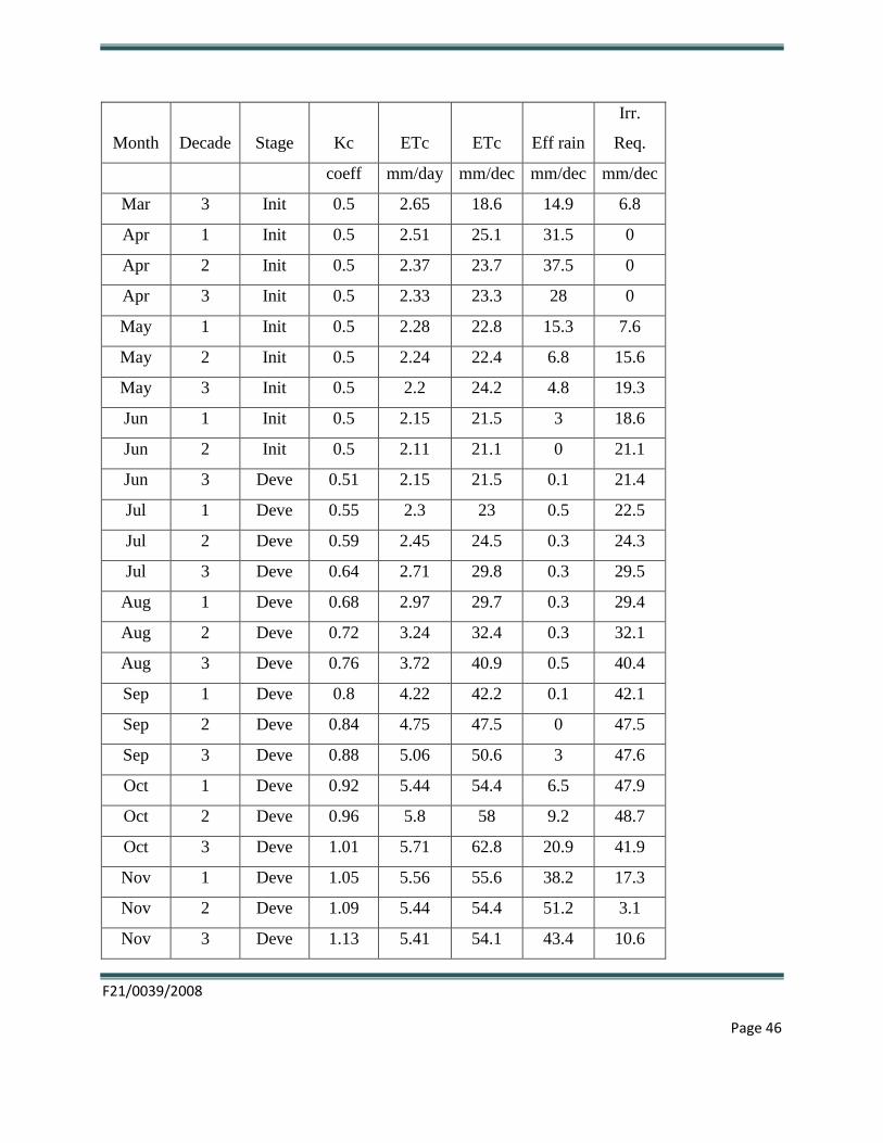
Table 5-6: Crop water Requirement for Banana
Crop water requirement is the water lost by the crop through evapo-transpiration when local
weather conditions are taken to account. Thaana Nzau irrigation system is in Agro-ecological
zone LM5. Here the design is based on flood irrigation assuming no rainfall is ever received in
the area.
The crops to be grown are horticultural crops ranging from deep-rooted to shallow rooted crops.
From the irrigation atlas of Kenya and CROPWAT analysis, the crop water requirement (Eto) for
Thana Nzau is 5.95mm/day
For horticultural crops, average crop factor = 0.9
Therefore, actual crop water requirement (Etc) = crop water requirement x crop factor
= 5.95mm/day x 0.9
= 5.4mm/day
Using a conversion factor of 0.116l/s-Ha ≡ 1mm/day
F21/0039/2008
Page 48
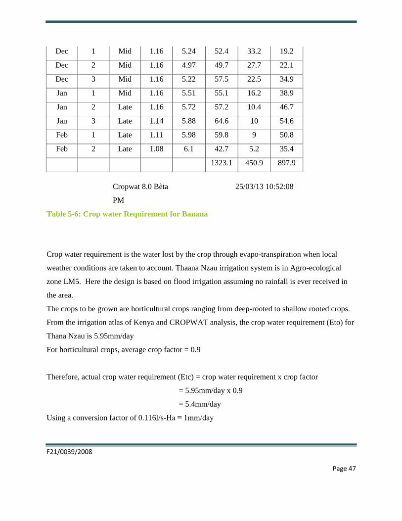
5.1.2 Net Irrigation Requirement (NIR)
The net irrigation requirement (NIR) has been determined as follows
NIR = ETcrop – Pe- Ge- Wb (mm/day)
Where, Pe is effective rainfall (mm)
Ge Ground water contribution (mm)
Wb Stored water contribution (mm), assumed negligible
From Table 5.2 above, Pe is
= 570/ (30*12) = 1.408 mm/day
Thus
Actual crop water requirement (NIR) =CWR x 0.116l/s-Ha
= (5.4 -1.4) x 0.116 l/s-Ha.
= 0.63l/s-Ha.
Determination of the overhead Tank capacity
Crops:
=0.63l/s-Ha * 10 Ha = 6.3l/s
Taking 8 hours per day for irrigation gives;
= 6.3 l/s * (8*3600) s
= 181,140 liters/day = 181.14 m3
F21/0039/2008
Page 49
Human Consumption:
Assuming;
Each of the 20 households has on average 6 persons
Each person uses 100 litres/day
= 20 households * 6 person * 100 l/day
= 12000 l/d
Animal consumption:
Assuming;
Each household has 5 livestock
Animal water consumption is 40 l/day
= 20 household * 5 livestock * 40 l/day
= 4000 l/day
Total Overhead Tank volume per day;
= 181.14 + 12000 + 4000 = 16,181.14 litres/day
= 20 m3
5.2 Canals Discharges
The canal flow rates are determined from the continuity equation;
Q = AV,
Where:
F21/0039/2008
Page 50
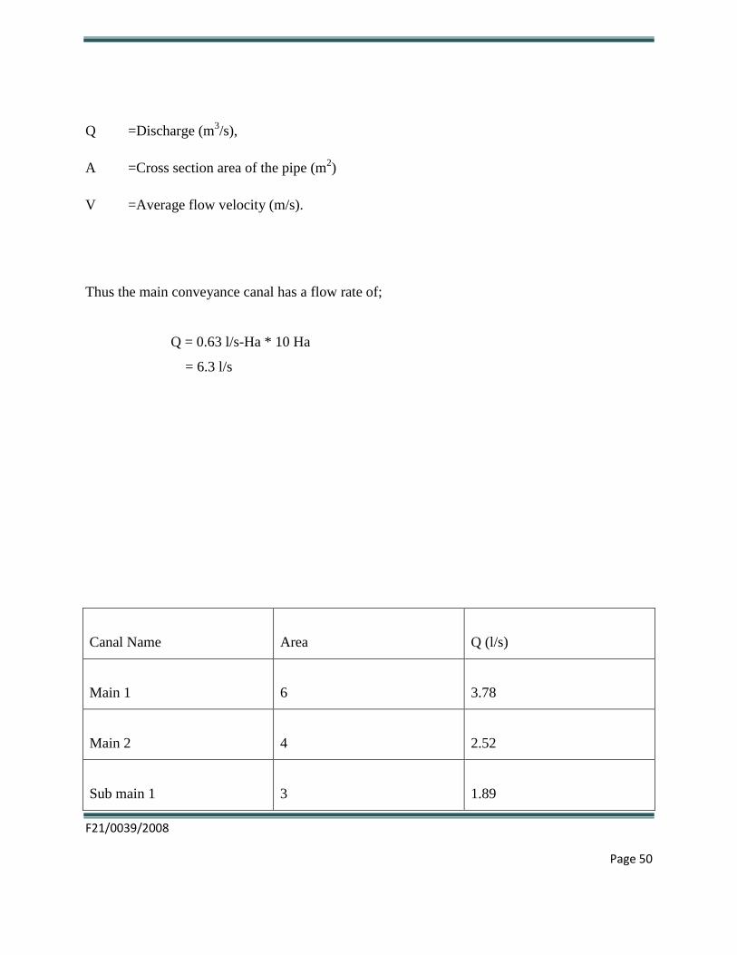
Q =Discharge (m3/s),
A =Cross section area of the pipe (m2)
V =Average flow velocity (m/s).
Thus the main conveyance canal has a flow rate of;
Q = 0.63 l/s-Ha * 10 Ha
= 6.3 l/s
Canal Name
Area
Q (l/s)
Main 1
6
3.78
Main 2
4
2.52
Sub main 1
3
1.89
F21/0039/2008
Page 51
Sub main 2
4
2.52
Sub main 3
2
1.26
Sub main 4
1
0.63
Feeder 1
2
1.26
Feeder 2
2
1.26
Feeder 2-1
1
0.63
Feeder 3
1
0.63
Feeder 3-1
1
0.63
Feeder 4
2
1.26
Feeder 5
1
0.63
Table 5-7: Canal flow rates
The flow rates in the table 8 were used to design the canals using spreadsheet.
F21/0039/2008
Page 52
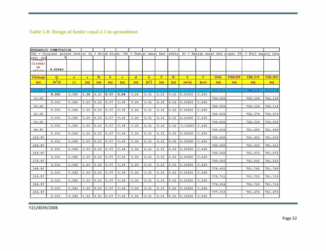
Table 5-8: Design of feeder canal 2-1 in spreadsheet
F21/0039/2008
Page 53
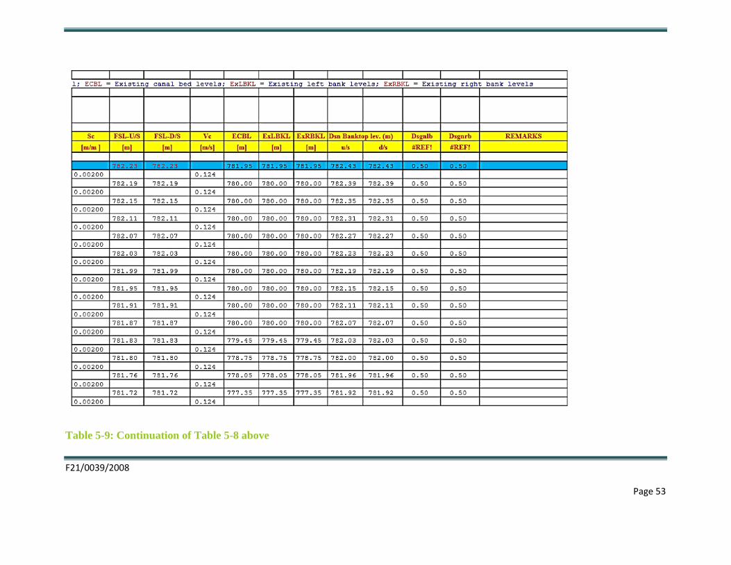
Table 5-9: Continuation of Table 5-8 above
F21/0039/2008
Page 54
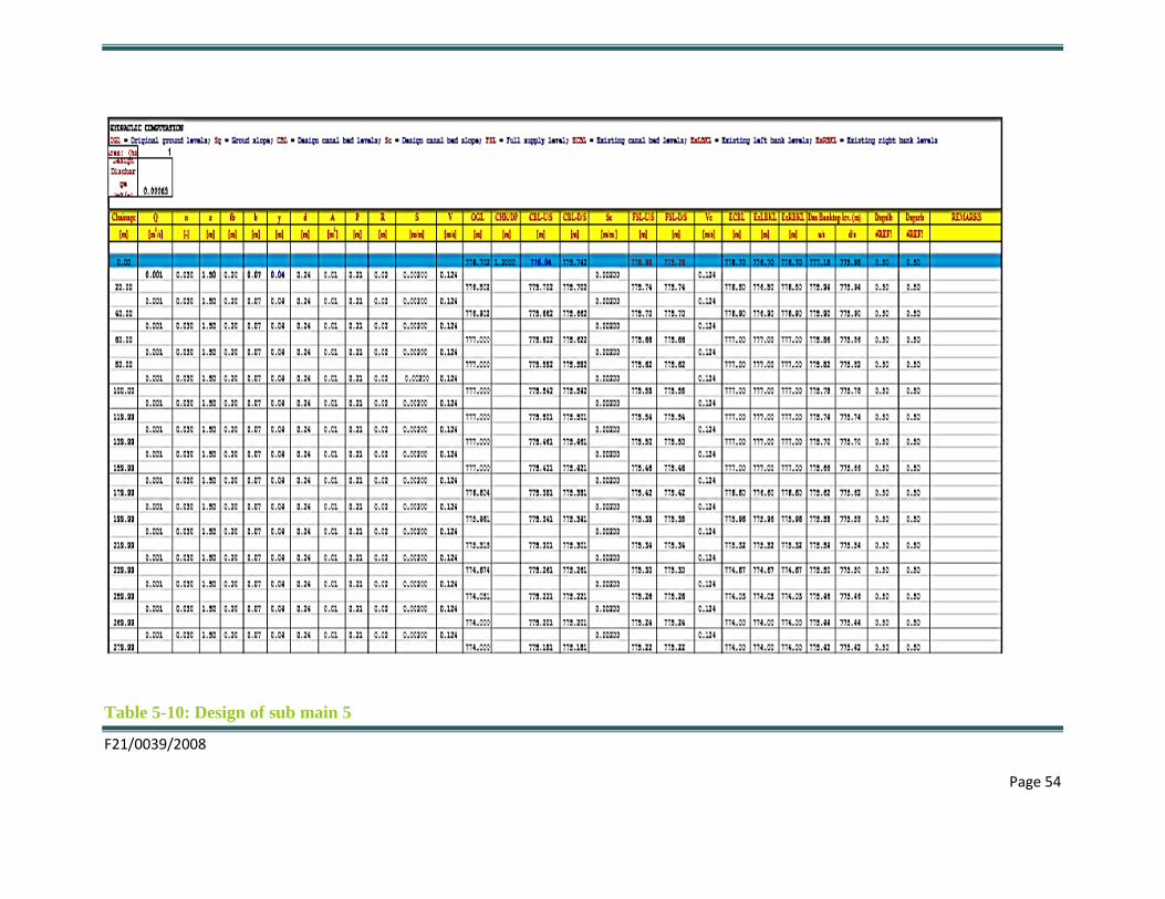
Table 5-10: Design of sub main 5
F21/0039/2008
Page 55
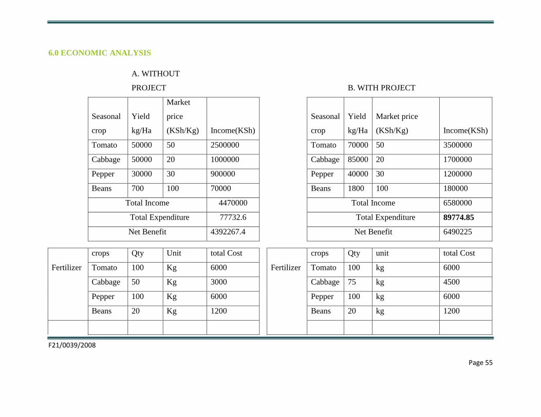
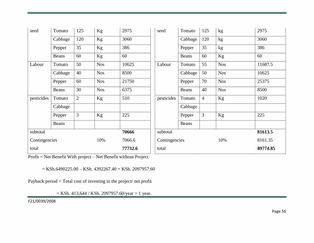
6.0 ECONOMIC ANALYSIS
A. WITHOUT
PROJECT
B. WITH PROJECT
Seasonal
crop
Yield
kg/Ha
Market
price
(KSh/Kg) Income(KSh)
Seasonal
crop
Yield
kg/Ha
Market price
(KSh/Kg) Income(KSh)
Tomato 50000 50 2500000
Tomato 70000 50 3500000
Cabbage 50000 20 1000000
Cabbage 85000 20 1700000
Pepper 30000 30 900000
Pepper 40000 30 1200000
Beans 700 100 70000
Beans 1800 100 180000
Total Income 4470000
Total Income 6580000
Total Expenditure 77732.6
Total Expenditure 89774.85
Net Benefit 4392267.4
Net Benefit 6490225
crops Qty Unit total Cost
crops Qty unit total Cost
Fertilizer Tomato 100 Kg 6000
Fertilizer Tomato 100 kg 6000
Cabbage 50 Kg 3000
Cabbage 75 kg 4500
Pepper 100 Kg 6000
Pepper 100 kg 6000
Beans 20 Kg 1200
Beans 20 kg 1200
F21/0039/2008
Page 56
seed Tomato 125 Kg 2975
seed Tomato 125 kg 2975
Cabbage 120 Kg 3060
Cabbage 120 kg 3060
Pepper 35 Kg 386
Pepper 35 kg 386
Beans 60 Kg 60
Beans 60 Kg 60
Labour Tomato 50 Nos 10625
Labour Tomato 55 Nos 11687.5
Cabbage 40 Nos 8500
Cabbage 50 Nos 10625
Pepper 60 Nos 21750
Pepper 70 Nos 25375
Beans 30 Nos 6375
Beans 40 Nos 8500
pesticides Tomato 2 Kg 510
pesticides Tomato 4 Kg 1020
Cabbage
Cabbage
Pepper 3 Kg 225
Pepper 3 Kg 225
Beans
Beans
subtotal
70666
subtotal 81613.5
Contingencies
10% 7066.6
Contingencies
10% 8161.35
total 77732.6
total 89774.85
Profit = Net Benefit With project – Net Benefit without Project
= KSh.6490225.00 – KSh. 4392267.40 = KSh. 2097957.60
Payback period = Total cost of investing in the project/ net profit
= KSh. 413,644 / KSh. 2097957.60/year = 1 year.
F21/0039/2008
Page 57
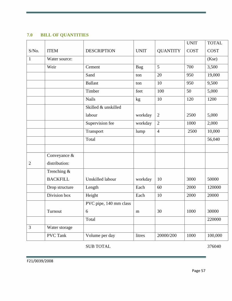
7.0 BILL OF QUANTITIES
S/No. ITEM DESCRIPTION UNIT QUANTITY
UNIT
COST
TOTAL
COST
1 Water source: (Kse)
Weir Cement Bag 5 700 3,500
Sand ton 20 950 19,000
Ballast ton 10 950 9,500
Timber feet 100 50 5,000
Nails kg 10 120 1200
Skilled & unskilled
labour workday 2 2500 5,000
Supervision fee workday 2 1000 2,000
Transport lump 4 2500 10,000
Total 56,040
2
Conveyance &
distribution:
Trenching &
BACKFILL Unskilled labour workday 10 3000 50000
Drop structure Length Each 60 2000 120000
Division box Height Each 10 2000 20000
Turnout
PVC pipe, 140 mm class
6 m 30 1000 30000
Total 220000
3 Water storage
PVC Tank Volume per day litres 20000/200 1000 100,000
SUB TOTAL
376040
F21/0039/2008
Page 58
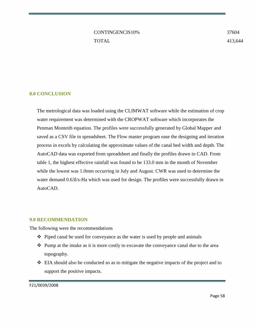
CONTINGENCIS10%
37604
TOTAL
413,644
8.0 CONCLUSION
The metrological data was loaded using the CLIMWAT software while the estimation of crop
water requirement was determined with the CROPWAT software which incorporates the
Penman Monteith equation. The profiles were successfully generated by Global Mapper and
saved as a CSV file in spreadsheet. The Flow master program ease the designing and iteration
process in excels by calculating the approximate values of the canal bed width and depth. The
AutoCAD data was exported from spreadsheet and finally the profiles drawn in CAD. From
table 1, the highest effective rainfall was found to be 133.0 mm in the month of November
while the lowest was 1.0mm occurring in July and August. CWR was used to determine the
water demand 0.63l/s-Ha which was used for design. The profiles were successfully drawn in
AutoCAD.
9.0 RECOMMENDATION
The following were the recommendations
Piped canal be used for conveyance as the water is used by people and animals
Pump at the intake as it is more costly to excavate the conveyance canal due to the area
topography.
EIA should also be conducted so as to mitigate the negative impacts of the project and to
support the positive impacts.
F21/0039/2008
Page 59
Chapter 10
10.0 REFERENCES
Clark M. W, Varma G. R, & Yates R. A. (1986). Irrigation Practices: Peasant-Farming
Settlement Schemes and Traditional Cultures. Retrieved from rsta.royalsocietypublishing.org
FAO $ SAFR. (2001). Irrigation Manual; Planning, Development monitoring and evaluation of
Irrigated Agriculture with Farmer participation, 3.
Frankline M. (1998). Dryland farming: Crops and Techniques for arid regions. ECHO Staff.
Gawaher M., & Amin M. S. (2005). Irrigation planning using geographic information system: A
case study of Sana’a Basin, Yemen. Management of Environmental Quality, 16(4), 347 – 361.
IlyamukuruL P. A., & Iyamuremye J. D. (2011). Sprinkler Irrigation Systems design project
Bugesera Community.
James, L.G. 1988. Principles of farm irrigation system design
Jensen, M.E. 198. Design and operation of farm irrigation systems.American Society of
Agricultural Engineers, U.S.A.
Kay, M. 1986. Surface irrigation - systems and practice.Cranfield Press, Bedford, U.K.
Keller, J. and Bliesner, R.D. 1990. Sprinkler and trickle irrigation. Chapman and Hall, New York.
Kraatz, D.B. and Stoutjesdijk, J.A. 1984. Improved headworks for reduced sediment
intake.Proceedings African Regional Symposium on Small Holder Irrigation, Harare.

F21/0039/2008
Page 60
L. K. Joshi and V. S. Dinkar, eds., Ministry of Water Resource, Government of India, New Delhi,
209–236. (FHWA, 1971)Hydraulic Engineering Circular No. 9, Debris Control Structures Knox
County Tennessee Stormwater Management Manual, Volume 2 (Technical Guidance)
Larry, J. 1988. Principles of farm irrigation system design. John Wiley and Sons.
Meteorological department, Dagorety (2010).Mwingi station weather data.
Rekha N., & Jayakumara M. A. (2010). Chapter 7 Progress of research on cascade irrigation
systems in the dry zones of Sri Lanka. Water Communities (Community, Environment and
Disaster Risk Management (Vol. 2, pp. 109 – 137). Emerald Group Publishing Limited,.
Retrieved from www.emerald.com
Wai F.L. (2006). Designing institutions for irrigation management: Comparing irrigation
agencies in Nepal and Taiwan (Vol. Vol. 24). Property Management,. Retrieved from
www.emerald.com
F21/0039/2008
Page I
11.0 APENDIX
11.1 PICTURES
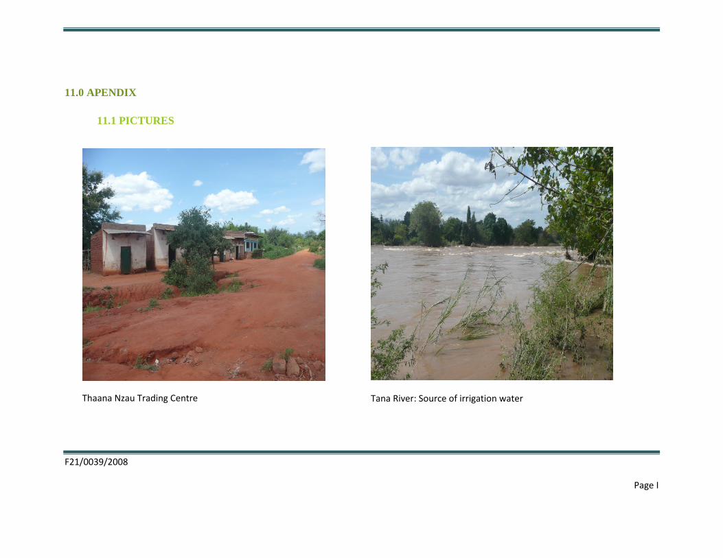
Thaana Nzau Trading Centre
Tana River: Source of irrigation water
F21/0039/2008
Page II
11.2 LOCATION MAP
11.3 CANAL LAYOUT
11.4 SOIL MAP
11.5 CONVEYANCE CANAL PROFILE (3 PARTS)
11.6 SUB MAIN 5 PROFILE (2 PARTS)
11.7 FEEDER 2-1 PROFILE