Journal of Manufacturing Systems ( ) –

Contents lists available at ScienceDirect

Journal of Manufacturing Systems

journal homepage: www.elsevier.com/locate/jmansys

Technical paper

Design of reconfigurable manufacturing systems

Yoram Koren a,∗,1, Moshe Shpitalni ba The University of Michigan, Ann Arbor, USAb Dean, Irwin and Joan Jacobs Graduate School, Technion, Israel Institute of Technology, Haifa, Israel

a r t i c l e i n f o

Article history:Received 3 January 2011Accepted 3 January 2011Available online xxxx

a b s t r a c t

This paper explains the rationale for the development of reconfigurable manufacturing systems, whichpossess the advantages both of dedicated lines and of flexible systems. The paper defines the corecharacteristics and design principles of reconfigurable manufacturing systems (RMS) and describesthe structure recommended for practical RMS with RMS core characteristics. After that, a rigorousmathematical method is introduced for designing RMS with this recommended structure. An exampleis provided to demonstrate how this RMS design method is used. The paper concludes with a discussionof reconfigurable assembly systems.

© 2011 The Society of Manufacturing Engineers. Published by Elsevier Ltd. All rights reserved.

1. Introduction

It is well known that Henry Ford’s invention of the movingassembly line in 1913 marked the beginning of the massproduction paradigm. Yet it is less known that mass productionwas made possible only through the invention of dedicatedmachining lines that produced the engines, transmissions andmain components of automobiles. Such dedicated manufacturinglines have a very high rate of production for the single part typethey produce, and they are very profitable when demand for thispart is high. These dedicated transfer lineswere themost profitablesystems for producing large quantities of products until the mid-1990s.

The invention of NC, and later CNC in the 1970s [1], facili-tated creation of flexiblemanufacturing systems (FMS) in the early1980s. Stecke and Solberg were the first to formalize amathemati-cal solution for flexible systems [2]; already in 1981 they describedthe operation policies of FMS for a job shop consisting of nine ma-chines interconnected by an automatic material handling mecha-nism [3]. Due to the high initial investment cost, however, close totwenty years elapsed before flexible manufacturing systems wereable to penetrate the transportation powertrain industry, which isthe largest market for FMS. At that time, in the 1980s and 1990s,the strategic goals ofmanufacturing enterpriseswere productivity,quality and flexibility [4].

In the mid-1990s, enhanced globalization and worldwidecompetitionmade it clear that FMSprovide only a partial economic

∗ Corresponding author.E-mail address: ykoren@umich.edu (Y. Koren).

1 James J. Duderstadt Distinguished University Professor of Manufacturing.

solution in a competitive market. The typical FMS serial structureused in industry (though not in job shops) facilitated changes inproducts manufactured, but it yielded a relatively slow productionrate anddidnot provide the volume flexibility for responding to theunexpected changes in demand resulting from global competition.Cochran [5] noted that manufacturing system designs must becapable of satisfying a company’s strategic objectives. Whendemand fluctuates, the strategic objective is to meet demand.This can only be accomplished by up-scaling or down-scaling thesystem’s physical structure. But cost effective scalability throughmodifications in the system’s physical cannot be accomplishedwith traditional FMS.

In response, in 1995 the University of Michigan submit-ted a proposal to NSF for establishing a research center onReconfigurable Manufacturing Systems [6]. This paper explainsthe characteristics and principles of reconfigurable manufactur-ing systems (RMS) that were proposed in 1995, compares RMSstructure with that of traditional flexible lines, and describesa mathematical method that facilitates RMS design. An exam-ple is provided to demonstrate how this RMS design method isused.

2. Manufacturing responsiveness is the challenge of globaliza-tion

Manufacturing companies in the 21st century face increasinglyfrequent and unpredictable market changes driven by globalcompetition, including the rapid introduction of new productsand constantly varying product demand. To remain competitive,companies must design manufacturing systems that not onlyproduce high-quality products at low cost, but also allow for rapid

0278-6125/$ – see front matter© 2011 The Society of Manufacturing Engineers. Published by Elsevier Ltd. All rights reserved.doi:10.1016/j.jmsy.2011.01.001

2 Y. Koren, M. Shpitalni / Journal of Manufacturing Systems ( ) –

response to market changes and consumer needs. Responsivenessrefers to the speed at which a plant can meet changing businessgoals andproducenewproductmodels. Reconfigurability is a novelengineering technology that facilitates cost effective and rapidresponses to market and product changes.

Responsiveness enables manufacturing systems to quicklylaunch new products on existing systems, and to react rapidly andcost-effectively to:

1. Market changes, including changes in product demand.2. Product changes, including changes in current products and

introduction of new products.3. System failures (ongoing production despite equipment fail-

ures).

All these changes are driven by aggressive competition on aglobal scale, customers who are more educated and demanding,and a rapid pace of change in product and process technology [7].

Although flexible manufacturing systems (FMS) do respond toproduct changes, they are not designed for structural changes [8]and therefore cannot respond to abrupt market fluctuations, suchas varying demand and major equipment failures.

The speed of responsiveness is a new strategic goal formanufacturing enterprises. Although responsiveness has not yetbeen attributed the same level of importance as cost and quality,its impact is quickly becoming equally imperative. Responsivenessprovides a key competitive advantage in a turbulent globaleconomy in which companies must be able to react to changesrapidly and cost-effectively. Responsiveness can be achieved byinstalling a manufacturing system that has modest initial capacityand is designed to add production capacity as the market growsand to add functionality as the product changes.

A responsive manufacturing system is one whose productioncapacity is adjustable to fluctuations in product demand, andwhose functionality is adaptable to new products. Therefore,two basic types of reconfiguration capabilities are needed inmanufacturing systems—in functionality (some types of flexiblemanufacturing systems allow functionality changes) and inproduction capacity. Fig. 1 shows how the actual demand forProducts A and B can differ from what was planned.

System production capacity must be adjusted to cope withfluctuations in product demand. This type of adjustment requiresrapid changes in the system’s production capacity, also referred toas system scalability [9].

Traditional manufacturing systems – both dedicated lines andFMS – are ill suited to meet the requirements dictated by thenew competitive environment. Dedicated manufacturing lines(DMLs) are based on inexpensive fixed automation that producesa company’s core products or parts over a long period and athigh volume, as seen in Fig. 2. Each dedicated line is typicallydesigned to produce a single part at a high rate of productionachieved by utilizing all tools simultaneously. When productdemand is high, the cost per part is particularly low. DMLsare cost effective as long as they can operate at full capacity,but with increasing pressure from global competition and over-capacity worldwide, dedicated lines usually do not operate at fullcapacity.

Flexible manufacturing systems (FMS) can produce a variety ofproducts with a changeable mix on the same system. Typically,FMS consist of general-purpose computer-numerically-controlled(CNC) machines and other programmable forms of automation.Because CNC machines are characterized by single-tool operation,FMS throughput is much lower than that of a DML. Thecombination of high equipment cost and low throughput makesthe cost per part using FMS relatively high. Therefore, FMS

production capacity is usually much lower than that of dedicatedlines (see Fig. 2).

3. RMS—a new class of systems

A cost effective response to market changes requires a newmanufacturing approach. Such an approach not only must com-bine the high throughput of a DML with the flexibility of FMS,but also be capable of responding to market changes by adapt-ing the manufacturing system and its elements quickly and ef-ficiently. These capabilities are encompassed in reconfigurablemanufacturing systems (RMS), whose capacity and function-ality can be changed exactly when needed, as illustrated inFig. 2.

Three features – capacity, functionality, and cost – are whatdifferentiate the three types of manufacturing systems — RMS,DML and FMS. While DML and FMS are usually fixed at thecapacity-functionality plane, as shown in Fig. 2, RMS are notconstrained by capacity or by functionality, and are capable ofchanging over time in response to changingmarket circumstances.

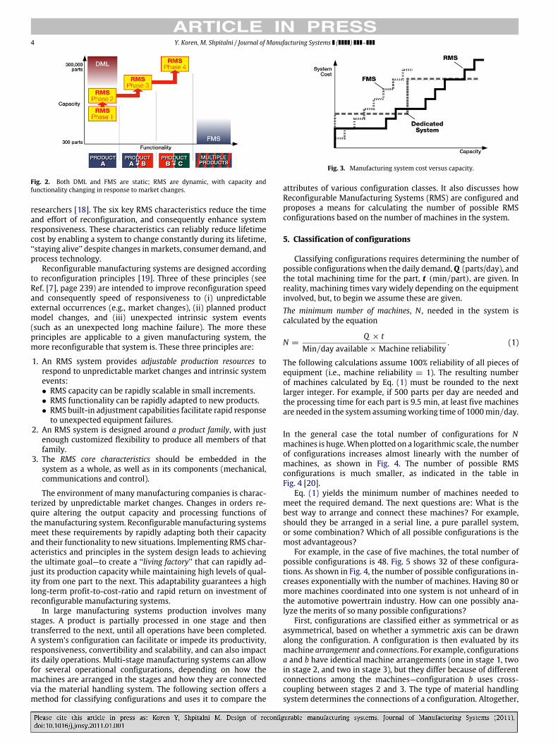
When taking systemcost versus capacity into consideration, theDML remains constant at its maximum planned capacity; an entireadditional linemust be built when greater capacity is needed. Pureparallel FMS are scalable at a constant rate (adding machines inparallel), as depicted in Fig. 3. But as Lee and Stecke stated [10],FMS are expensive: ‘‘FMS require large capital investment, and alarge portion of this investment is committed at the early designstage’’. RMS are scalable, but at non-constant steps that depend oninitial design and market circumstances.Manufacturing equipment is reconfigurable if the answer to thefollowing two questions is positive.

1. Was this manufacturing system or equipment designed so thatits physical structure can be easily changed?

2. Was this manufacturing system or equipment designed forproduction or inspection of a particular part family?

Examples of changes in a system’s physical structure includeadding a new production resource rapidly and in a cost effectivemanner (e.g., a new CNC machine or conveyor extension),changing a tool magazine or changing the direction of an axis ofmotion.

FMS have the flexibility needed to switch between productvariants in manufacturing, but are not as cost effective as DMLs. Bycontrast, a DML is marked by high productivity but no flexibility. Areconfigurable manufacturing system embraces the best qualitiesof both types. Not only is it cost effective with flexible productioncapabilities, but its structure also can be changed at both thesystem level and the machine level, so it can handle unexpectedmarket changes [11].

DML design focuses on the specific part to be produced. Thus,if a part is not defined, a DML cannot be designed. By contrast,typical FMS are composed of CNC machines and are designed tomanufacture any part (within an envelope). A process-planningprocedure is needed to fit the processing of each specific part tothe existing FMS. FMS design focuses on the machine rather thanon the part, which is one reason for the waste and low productionrates of FMS technology.

Borrowing from dedicated lines that are designed around asingle part/product, RMS systems focus on families of parts, such ascylinder heads of car engines. Four-, six- and eight-cylinder engineshave many differences, but they also have many more features incommon. Focusing on the part family enables a designer to plana system that accommodates different variations of the same partfamily with minimum alteration to the production scheme. Thisapproach utilizes the high productivity of DML machine design,

Y. Koren, M. Shpitalni / Journal of Manufacturing Systems ( ) – 3

Fig. 1. Projection compared to actual product demand: Higher initial demand than expected for both products, and product C is introduced earlier than expected.

Table 1RMS systems combine features of dedicated and flexible systems.

Dedicated RMS/RMT FMS/CNC

System structure Fixed Changeable Changeable

Machine structure Fixed Changeable Fixed

System focus Part Part family Machine

Scalability No Yes Yes

Flexibility No Customized (around a part family) General

Simultaneously operating tools Yes Possible No

Productivity Very high High Low

Cost per part Low (For a single part, when fully utilized) Medium (Parts at variable demand) Reasonable (Several parts simultaneously)

and is much more economical than the general functionality ofFMS.

As summarized in Table 1, Reconfigurable ManufacturingSystems (RMS) constitute a new class of systems characterized byadjustable structure and design focus.

A system built with changeable structure provides scalabilityand customized flexibility and focuses on a part family, thusgenerating a responsive reconfigurable system. The flexibility ofRMS, though really only ‘‘customized flexibility’’, provides all theflexibility needed to process that entire part family.

Highly productive, cost effective systems are created by(i) part-family focus, and (ii) customized flexibility that enables thesimultaneous operation of different tools [12]. RMS systems are de-signed to cope with situations where both productivity and sys-tem responsiveness are of vital importance. Each RMS system isdesigned to produce a particular family of parts. The main com-ponents of RMS for machining are CNC machines and Reconfig-urable Machine Tools [13]. Reconfigurable controls integrated inan open-architecture environment that can coordinate and operatethe CNCs and RMTs are critical to RMS success [14]. Therefore, a re-configurable manufacturing system can be defined as follows [15]:

Reconfigurable Manufacturing Systems (RMS) are designed at theoutset for rapid change in structure, as well as in hardware andsoftware components, in order to quickly adjust production capacityand functionality within a part family in response to sudden changesin market or regulatory requirements.

If the system and its machines are not designed at the outset forreconfigurability, the reconfiguration process will prove lengthyand impractical.

4. Characteristics and principles of reconfiguration

RMS are marked by six core reconfigurable characteristics, assummarized below [16].

Customization (flexibilitylimited to part family)

System or machine flexibilitylimited to a single productfamily, thereby obtainingcustomized flexibility

Convertibility (design forfunctionality changes)

The ability to easily transformthe functionality of existingsystems and machines to suitnew production requirements

Scalability (design forcapacity changes)

The ability to easily modifyproduction capacity by adding orsubtracting manufacturingresources (e.g. machines) and/orchanging components of thesystem

Modularity (componentsare modular)

The compartmentalization ofoperational functions into unitsthat can be manipulated betweenalternate production schemes foroptimal arrangement

Integrability (interfaces forrapid integration)

The ability to integrate modulesrapidly and precisely by a set ofmechanical, informational, andcontrol interfaces that facilitateintegration and communication

Diagnosability (design foreasy diagnostics)

The ability to automatically readthe current state of a system todetect and diagnose the rootcauses of output product defects,and quickly correct operationaldefects

Customization, scalability and convertibility [17] are critical re-configuration characteristics. Modularity, integrability and diag-nosability allow rapid reconfiguration, but they do not guaranteemodifications in production capacity and functionality. Customiza-tion, an essential RMS characteristic, is based upon design for a partfamily or a product family, a concept already mentioned by other

4 Y. Koren, M. Shpitalni / Journal of Manufacturing Systems ( ) –

Fig. 2. Both DML and FMS are static; RMS are dynamic, with capacity andfunctionality changing in response to market changes.

researchers [18]. The six key RMS characteristics reduce the timeand effort of reconfiguration, and consequently enhance systemresponsiveness. These characteristics can reliably reduce lifetimecost by enabling a system to change constantly during its lifetime,‘‘staying alive’’ despite changes inmarkets, consumer demand, andprocess technology.

Reconfigurable manufacturing systems are designed accordingto reconfiguration principles [19]. Three of these principles (seeRef. [7], page 239) are intended to improve reconfiguration speedand consequently speed of responsiveness to (i) unpredictableexternal occurrences (e.g., market changes), (ii) planned productmodel changes, and (iii) unexpected intrinsic system events(such as an unexpected long machine failure). The more theseprinciples are applicable to a given manufacturing system, themore reconfigurable that system is. These three principles are:

1. An RMS system provides adjustable production resources torespond to unpredictable market changes and intrinsic systemevents:• RMS capacity can be rapidly scalable in small increments.• RMS functionality can be rapidly adapted to new products.• RMS built-in adjustment capabilities facilitate rapid response

to unexpected equipment failures.2. An RMS system is designed around a product family, with just

enough customized flexibility to produce all members of thatfamily.

3. The RMS core characteristics should be embedded in thesystem as a whole, as well as in its components (mechanical,communications and control).

The environment of many manufacturing companies is charac-terized by unpredictable market changes. Changes in orders re-quire altering the output capacity and processing functions ofthemanufacturing system. Reconfigurablemanufacturing systemsmeet these requirements by rapidly adapting both their capacityand their functionality to new situations. Implementing RMS char-acteristics and principles in the system design leads to achievingthe ultimate goal—to create a ‘‘living factory’’ that can rapidly ad-just its production capacity while maintaining high levels of qual-ity from one part to the next. This adaptability guarantees a highlong-term profit-to-cost-ratio and rapid return on investment ofreconfigurable manufacturing systems.

In large manufacturing systems production involves manystages. A product is partially processed in one stage and thentransferred to the next, until all operations have been completed.A system’s configuration can facilitate or impede its productivity,responsiveness, convertibility and scalability, and can also impactits daily operations. Multi-stage manufacturing systems can allowfor several operational configurations, depending on how themachines are arranged in the stages and how they are connectedvia the material handling system. The following section offers amethod for classifying configurations and uses it to compare the

Fig. 3. Manufacturing system cost versus capacity.

attributes of various configuration classes. It also discusses howReconfigurable Manufacturing Systems (RMS) are configured andproposes a means for calculating the number of possible RMSconfigurations based on the number of machines in the system.

5. Classification of configurations

Classifying configurations requires determining the number ofpossible configurationswhen the daily demand,Q (parts/day), andthe total machining time for the part, t (min/part), are given. Inreality, machining times vary widely depending on the equipmentinvolved, but, to begin we assume these are given.The minimum number of machines, N , needed in the system iscalculated by the equation

N =Q × t

Min/day available × Machine reliability. (1)

The following calculations assume 100% reliability of all pieces ofequipment (i.e., machine reliability = 1). The resulting numberof machines calculated by Eq. (1) must be rounded to the nextlarger integer. For example, if 500 parts per day are needed andthe processing time for each part is 9.5 min, at least five machinesare needed in the system assumingworking time of 1000min/day.

In the general case the total number of configurations for Nmachines is huge.When plotted on a logarithmic scale, the numberof configurations increases almost linearly with the number ofmachines, as shown in Fig. 4. The number of possible RMSconfigurations is much smaller, as indicated in the table inFig. 4 [20].

Eq. (1) yields the minimum number of machines needed tomeet the required demand. The next questions are: What is thebest way to arrange and connect these machines? For example,should they be arranged in a serial line, a pure parallel system,or some combination? Which of all possible configurations is themost advantageous?

For example, in the case of five machines, the total number ofpossible configurations is 48. Fig. 5 shows 32 of these configura-tions. As shown in Fig. 4, the number of possible configurations in-creases exponentially with the number of machines. Having 80 ormore machines coordinated into one system is not unheard of inthe automotive powertrain industry. How can one possibly ana-lyze the merits of so many possible configurations?

First, configurations are classified either as symmetrical or asasymmetrical, based on whether a symmetric axis can be drawnalong the configuration. A configuration is then evaluated by itsmachine arrangement and connections. For example, configurationsa and b have identical machine arrangements (one in stage 1, twoin stage 2, and two in stage 3), but they differ because of differentconnections among the machines—configuration b uses cross-coupling between stages 2 and 3. The type of material handlingsystem determines the connections of a configuration. Altogether,

Y. Koren, M. Shpitalni / Journal of Manufacturing Systems ( ) – 5

Fig. 4. Total number of system configurations for different numbers of machines.

Fig. 5. Configurations with five machines.

a system with five machines may have 16 different symmetricarrangements (13 of which are plotted in Fig. 5). Fortunately, thedesigner will consider only symmetric configurations.

Asymmetric configurations add immense complexity and arenot viable in real manufacturing lines, as explained below. Thenumber of possible asymmetric configurations is much larger thanof symmetric configurations—a total of 30 in the case of fivemachines (18 of them are plotted in Fig. 5). It is important to notethat configurations d′ and e′ are defined as asymmetric (althoughthey have a symmetric axis) because they may be positioneddifferently (as d and e). Similarly, according to reconfigurationscience, the two configurations f and g in Fig. 5 are definedas asymmetric configurations, although they may be drawn assymmetric.

We would like to explain why asymmetric configurations areusually not suitable for real machining systems (though they maybe suitable for assembly systems)? Asymmetric configurationsmay be sub-classified as (a) variable-process configurations or (b)single-process configurations with non-identical machines in atleast one of the stages. Corresponding examples are shown inFig. 6(a) and (b), respectively.

Variable-process configurations are characterized by possiblenon-identical flow-paths for the part. They therefore needseveral process plans and corresponding setups. For example, thesystem depicted in Fig. 6 has a number of possible flow-paths:a–b–c–d–e, g–c–f , g–c–d–e, etc. The process plan to be executeddepends on the flow-path of the part being processed in thesystem. This is absolutely impractical because (1) designers willnot go to the effort to design multiple process plans for the samepart, and (2) different process plans and corresponding flow-pathsincrease part quality problems and make quality error detectionmore complicated.

Although the process planning is identical in each flow-path inthe second class of asymmetric configurations, the machines aredifferent in at least one stage. For example, in Fig. 6(b), machine bin stage 2 must be two times faster than machines a; machine din stage 4 must be two times faster than machines c . In symmetricconfigurations, in contrast, the processing times of each machine

in a particular stage are equal. Mixing different types of machinesthat perform exactly the same sequence of tasks in the samemanufacturing stage is absolutely impractical. System designersshould also not consider this class of configuration, due to theirexcessive complexity. The conclusion is:

It ismore likely that in a realmachining context, only symmetricconfigurations would be considered; these are always single-process configurations with identical machines in each stage.

Symmetric configurations may be further divided into threebasic classes, as shown in Fig. 7.A designer of manufacturing systems should consider only thefollowing three classes:

I. Cell configurations are configurations consisting of several serialmanufacturing lines (i.e., cells) arranged in parallel with nocrossovers, as shown in Fig. 8. Cell configurations, commonlyused in Japan, are simple.

II. RMS configurations are configurations with crossover connec-tions after every stage, as shown in Fig. 9. A part from anymachine in stage i can be transferred to any machine in stage(i+1). All machines and operations in every stage are identical.All threeUSdomestic automobilemanufacturers use these con-figurations in the machining of their powertrain components(a typical system may consist of 15 stages and 6 machines perstage).

III. Configurations in which there are some stages with nocrossovers. This class includes combinations of the previoustwo classes.

Note that a mathematical model that minimizes inter-cellmaterial handling costs for equipment layout in a single cell hasbeen developed [21], but it has not been expanded to a systemwithseveral cells.

The sketch in Fig. 10 of a practical 3-stage RMS system withgantries that transport the parts illustrates the issue of RMSconfiguration. A spine gantry transfers a part to a small cellconveyor. The part then moves along the conveyor to a positionwhere a cell gantry can pick it up and take it for processing in one

6 Y. Koren, M. Shpitalni / Journal of Manufacturing Systems ( ) –

Fig. 6. Two classes of asymmetric configurations.

Fig. 7. Three classes of symmetric configurations.

Fig. 8. Symmetric configuration of Class I—parallel lines, or cells. (If the twomarkedmachines fail, the system production stops.)

Fig. 9. Symmetric configuration of Class II—RMS configuration. (If the two markedmachines fail, the system still has 50% production capacity.)

Fig. 10. A practical reconfigurable manufacturing system.

of the machines in its stage. When the part has been processed,the cell gantry returns the part to the conveyor, which moves thepart to a position at which the next spine gantry can pick it up forprocessing in the next stage, and so on.

6. Comparing RMS configurations with cell configurations

Below we compare the two main practical configurationsaccording to four criteria: investment cost, line-balancing ability,scalability options, and productivity when machines fail. For amore general analysis of the impact of configuration on systemperformance; see [22].Capital investment. The configurations shown in Figs. 8 and 9(or Fig. 10) have identical machine arrangements – three stageswith two machines in each stage – but the connections are quitedifferent in that they use different part handling devices, eachrequiring a different capital investment. The entire part handling

system in Fig. 8 is simpler and has a smaller number of handlingdevices compared to the RMS system shown in Fig. 10. Thus, thecapital investment in the RMS configuration is higher.Line balancing. A major drawback of cell configuration is thatit imposes severe limitations when balancing the system. Forexample, if just one product is produced, the processing timein all stages of the cell configuration must be exactly equal tobe perfectly balanced. By contrast, to achieve a balanced RMSconfiguration only the following relationship needs to be satisfied

ts1/Ns1 = ts2/Ns2 = tsi/Nsi (2)

where Nsi is the number of machines in stage i, and tsi isthe processing time per machine in stage i. Therefore, in RMSconfigurations the number ofmachines per stage is not necessarilyequal in all stages. The number of machines in the various stagesof RMS configurations may be adjusted to provide accurate linebalancing, which consequently yields improved productivity.System scalability. RMS configurations are far more scalable thancell configurations. Adding one machine to one of the stagesand rebalancing the system enables adding a small increment ofcapacity. In the cell configuration, a complete additional parallelline must be added to increase the overall system capacity.In markets with unstable demand, scalability represents animportant advantage of RMS configurations.Productivity. If machine reliability is low due to crossovers ateach stage, an RMS configuration offers higher productivity thanthat of a cell configuration. As shown in Fig. 8, if machines intwo different lines and at two different stages (marked with x)are down, the entire system is down (i.e., throughput = zero).For RMS, in contrast, under the same conditions – two machinesnot working (marked with x in Fig. 9) – throughput is still at50%. So, RMS are more productive systems from the perspectiveof machine downtime. Nevertheless, the RMS material handlingsystem is more complex, with its so-called ‘‘cell gantries’’ thatenable crossovers (see Fig. 10). If one of the cell gantries is down,the entire RMS system will not work. In contrast, cellular systemswith parallel lines do not contain cell gantries and are thereforemore reliable from the material handling system perspective.The consequent critical question is therefore: When consideringreliability, which configuration yields higher productivity?

A complete analysis of this problem is presented by Freiheitet al. [23,24]. In this analysis the number of machines per stage inthe RMS configuration is equal in all stages. The RMS configurationhas a spine gantry with reliability identical to that of the conveyorsin Fig. 8. The analysis calculates tradeoffs between cell-gantryreliability and machine reliability.

Y. Koren, M. Shpitalni / Journal of Manufacturing Systems ( ) – 7

Fig. 11. Productivity comparison between parallel lines and RMS configurations.

Fig. 11 shows one typical result plotted for gantry reliability (oravailability) of Gr = 0.96, and machine reliability of Mr = 0.90.Our analysis revealed a borderline based onmachine reliability andgantry reliability (which must always be better than the machinereliability). On the right-top side of the borderline, RMS withcrossovers are preferred. For example, if the systemhas nine stageswith four machines per stage, the RMS configuration will yieldhigher productivity than a parallel-line configuration. The parallel-line configuration is preferable when, for example, the systemhas nine stages with just two machines per stage (namely, twoparallel lines with nine stages). The better the machine averagereliability (e.g., 0.95), the larger the solution space for a parallel-line configuration (without crossovers), and vice versa.The main conclusions of this analysis are:

• In large systems, with a large number of stages and machinesper stage, the RMS configuration has higher productivity thanthe parallel-line configuration (i.e., cells).

• If machine reliability is very high, the cell configuration yieldshigher productivity.

The advantages of each configuration are summarized in the tablebelow.

Capitalinvestment

Scalability Linebalancing

Productivity

Parallellines

Lower Higher for highmachine reliability

RMSconfiguration

Muchbetter

Muchbetter

Higher in complex,large systems

7. Integrated RMS practical configurations

This section deals with two issues: (a) designing RMS systemswith all six core characteristics, and (b) designingRMS systems thatincorporate innovative reconfigurable machine tools (RMTs) andreconfigurable inspection machines (RIMs) into the configuration.These two innovationsmake RMSmore productive and responsive.

Our starting point is the RMS configuration depicted inFig. 12, representing a system already utilized in the powertrainindustry. This three-stage system can produce two different partssimultaneously. A cell gantry serves all machines in a particularstage, bringing parts and loading themon themachines, and takingthe finished parts and transferring them to a buffer (the circlein Fig. 12) located next to the main material handling system.This system is usually a gantry (called the spine gantry), but canalso be a conveyor or several AGVs [25]. To balance the systemsequence, all stages should have almost the same cycle time. Inthis figure, the cycle time for each of the two machines in stage2 is approximately two-thirds of the cycle time for the three

machines in stages 1 and 3. (In industry, the set of all machiningtasks assigned to a stage is called an ‘‘Operation’’. Operations areusually assigned the numbers 10, 20, 30, etc., allowing for theaddition of intermediate operations as needed over time, as inadding Operation 15. Here we prefer the term ‘‘stage’’.)The system in Fig. 12 has four of the six core RMS characteristics:

Modularity: At the system level, each CNC machine is a module.Integrability: Machines at the same stage are integrated via cell

gantries, which, in turn, are integrated into a completesystem by a conveyor or spine gantries or AGVs. (Thecircles in Fig. 12 represent buffers.)

Scalability: Machines can be easily added at each stage withoutinterrupting system operation for long periods. Froma system-balancing viewpoint, scalability begins at thestages that are already bottlenecks to reduce systemcycletime.

Convertibility: It is easy to stop the operation of one CNC at a timeand to reconfigure its functionality to produce a new typeof part.

Scalability and convertibility enhance overall system performance.The system in Fig. 12, however, does not yet have the two remain-ing characteristics: customization (i.e., part family customized flex-ibility) and diagnosability.

As mentioned, implementing customized flexibility is criticalto increasing productivity. Introducing this characteristic into areconfigurable system is the key to enhance productivity, but howexactly can this be accomplished?

Let us assume that the milling tasks on the machined partcan be separated from the drilling and tapping tasks and thatmilling can be assigned to different stages than drilling and tapping(i.e., performed in different stages in the system). The drillingand tapping tasks for a particular part α can be done very fast(at a dedicated machine speed) on a reconfigurable machine tool(RMTα) that is capable of drilling (or tapping) multiple holessimultaneously, on a particular part α in a single stroke—a singlemotion of the Z-axis. RMTα is customized to part α. Two RMTs,for two parts α and β are integrated into the configurationshown in Fig. 13. Namely, customization has been embeddedinto this system, resulting in a dramatic improvement in systemthroughput.

The sixth characteristic, diagnosability, can be embedded ifthe system includes in-process inspection resources that allowdetection of quality defects in real time. In practice, this isimplemented by installing reconfigurable inspection machines(RIMs) at a separate stage in the system, which allows theinspection to be conducted in a contaminant-free environmentand can be bypassed if necessary, as shown in Fig. 13. Performingin-process diagnostics has a double advantage: it dramaticallyshortens the ramp-up periods after reconfigurations, and itallows rapid identification of part quality problems during normalproduction.

8. Calculating the number of RMS configurations

Professor Nam Suh laid out a theoretical framework for thedesign of large systems [26]. Yet as he himself wrote, ‘‘the goalis to develop a thinking design machine and create pedagogicaltools for teaching’’. A few years later, Jacobsen et al. [27]recognized that ‘‘the design of a production system is a challengingactivity’’. Yet the authors of this article did not propose amathematical method or even a design procedure. Here wepropose a practicalmathematicalmethod that engineers can easilyutilize for designing reconfigurable manufacturing systems.

We have already seen that the minimum number of machinesN required in the system can be easily calculated by solving

8 Y. Koren, M. Shpitalni / Journal of Manufacturing Systems ( ) –

Fig. 12. Practical RMS configuration with three stages.

Fig. 13. RMS with integrated RMTs and RIMs.

Eq. (1). However, as shown in Fig. 5, the number of all possibleconfigurations with N machines is enormous. After a thoroughmathematical study of system configurations, we conclude thefollowing:Closed equations for calculating the number of configurations with Nmachines exist only for RMS-type configurations.

The basic equations for calculating the number of possible RMSconfigurations are given below. K , the number of possible RMSconfigurations with N machines arranged in up to m stages iscalculated by:

K =

N−m=1

N − 1m − 1

= 2N−1 (3)

K , the number of possible configurations with N machinesarranged in exactly m stages is calculated by:

K =

(N − 1)!

(N − m)!(m − 1)!

. (4)

For example, for N = 7 machines arranged in up to 7 stages,Eq. (3) yields K = 64 configurations, and if arranged in exactly 3stages, Eq. (4) yieldsK = 15 RMS configurations. Themathematicalresults of these two equations for any N andmmay be arranged ina triangular format, known as a Pascal triangle, shown in Fig. 14.The numerical value of each cell in the Pascal triangle is calculatedas follows. The numerical value corresponding to N machinesarranged in m stages is calculated by:

The value for N machines in m stages = (the value for N − 1machines in m − 1 stages) + (the value for N − 1 machines in mstages).For example, in Fig. 14, the cell ofN = 5 andm = 3 shows 6, whichis the sum of 3+ 3 of the previous line ofN−1 = 4machines with2 and 3 stages.

The triangle also allows the designer to immediately visualizethe number of possible RMS configurations for N machines

Fig. 14. The Pascal triangle is helpful in calculating the number of RMSconfigurations.

arranged inm stages. For example, there are 15 RMS configurationswhen 7 machines are allowed to be arranged in exactly 3stages. In addition, the Pascal triangle allows the designer toimmediately calculate the number of possible RMS configurationsfor N machines arranged between i stages and j stages (i, j < N).This information is used in the following example.

9. Example of system design

The following example demonstrates how the Pascal Trianglein Fig. 14 can be used to design a machining system with RMSconfiguration.

Raw parts are brought to a machining system after casting. Thesystem contains many CNC machines that perform all machiningoperations required to finish the part, including milling, drilling,tapping, etc. A typical part of an automobile powertrain system isshown in Fig. 15. Note that the part has to be machined on severalfaces, and that there are more than 200 machining tasks required

Y. Koren, M. Shpitalni / Journal of Manufacturing Systems ( ) – 9

Fig. 15. An engine part after machining.

Fig. 16. Machining times.

to complete such a part, so it is impractical to include them all inthis demonstration.For simplicity, we consider a part that requires work on two facesonly. Each face requires separate fixturing, and therefore the twofaces must be machined using two separate setups. Our simplifiedexample requires only five machining tasks to be completed. Buteven in this simple example, the analysis is tedious and lengthy.Themethodical approach presented below is used to whittle downthe range of possibilities and make logical decisions based on factsand data to determine the optimal system configuration.The problem to be solved is defined as:Design a machining system to machine a part that requires t =

12.2 min of machining time in five machining tasks. The executiontimes for the five tasks are given in Fig. 16. The required daily volumeis Q = 500 parts/day.The working time per day is 1000 min. Machine reliability isassumed to be 100%.Solution: Producing 500 parts in 1000 min requires a cycle time of2min per part. The first step is to determine theminimumnumberofmachines needed. Eq. (1) yields 6.1machines. This numbermustbe rounded to the next integer, so that N = 7 machines.

According to Eq. (3), 7 machines and possible stages rangingfrom 1 to 7 yield 64 configurations to analyze. This large numberof configurations can be reduced by considering the specific tasks.Since the part has only 5 machining tasks, the maximum numberof stages can be 5. The part has two faces, each requiring a differentset-up; therefore, the minimum number of stages must be 2. ThePascal triangle in Fig. 14 indicates that 7 machines in the 2–5 stagerange have only 56 configurations.

But do we really have to compare all 56 configurations? Theanswer is no! If the part has two faces, we can divide the systeminto two sub-systems – one for Face 1 and the other for Face 2 – andthen design two separate sub-systems. In the Face 1 sub-system,the machining time t is 3.7 min per part. According to Eq. (1) therequired number of machines for Face 1 is 2.

N =500 × 3.7

1000= 1.85 ⇒ 2 machines. (5a)

In the Face 2 sub-system, the machining time t is 8.5 min per part.According to Eq. (1) the required number of machines for Face 2

Fig. 17. Pascal triangle for the example.

Fig. 18. Two stages.

is 5.

N =500 × 8.5

1000= 4.25 ⇒ 5 machines. (5b)

The Pascal triangle for these two sub-systems in Fig. 17 reveals only15 possible configurations (rather than 56): one for Face 1, and 15for Face 2.

The calculation yields: 1 × (1 + 4 + 6 + 4) = 15.

• If the system contains only two stages, there is only one possibleconfiguration: stage 1 with two machines for Face 1, and stage2 with five machines for Face 2.

• If the system comprises three stages, there are four possibleconfigurations.

• For four stages there are six possible configurations.• For five stages there are four configurations: stage 1 for Face 1,

and 4 stages for Face 2.

The formula for calculating the number of machines in Eq. (1),however, is based on a perfectly balanced system,while the systemhere is not necessarily balanced. Therefore, several of these 15possible configurations will not meet the demand of 500 parts perday. Our next step is to determine which of the configurations willnot meet the demand and then to eliminate them.

• For two stages there is only one possible configuration, theone depicted in Fig. 18. In stage 1, one part is produced every1.85 min (between the two machines), and in stage 2 one partis produced (between the five machines) every 1.7 min. Stage1 is the bottleneck and dictates that the system cycle time istmax = 1.85 min. The number of parts per day is therefore:Q = 1000/tmax = 540.

• For three stages, there are four possible configurations. However,only three of these satisfy the cycle time constraint of tmax ≤

2 min. The three systems are depicted in Fig. 19. In these threecases, the cycle time is tmax = 1.85 min.The fourth configuration (not shown) has only one machinein the third stage, which becomes a bottleneck with a cycletime of 3.3 min and cannot satisfy the required demand (aminimum cycle time of 2 min). Therefore, that configuration isunacceptable.

10 Y. Koren, M. Shpitalni / Journal of Manufacturing Systems ( ) –

Fig. 19. Configurations with three stages.

Fig. 20. Configurations with four stages.

• For four stages there are six possible configurations. However,three of them do not satisfy the cycle time constraint of tmax ≤

2 min and have been eliminated from consideration. The threeacceptable systems shown in Fig. 20 have a cycle time of tmax =

1.85 min. The three eliminated configurations have only onemachine in the fourth stage, which becomes a bottleneck witha cycle time of 3.3 min and cannot meet the required demand.

• For five stages there are four possible configurations, butonly one of them (Fig. 21) is valid. The bottleneck in thisconfiguration is in the third stage, which yields a cycle timeof 2 min. In the other three five-stage configurations, only onemachine is placed in the fifth stage, an arrangement that doesnot satisfy the required cycle time.

Because of the cycle time requirement, the number of configura-tions is reduced from 15 to 8. Altogether, the number of possi-ble RMS configurations to consider has been reduced from 64 to8. Eight configurations is a manageable number to compare.In order to make a final decision, the designer has to consider atleast the following four factors (ranked by importance):

1. System throughput with reliability less than 100% (see nextsection).

2. Investment cost.3. Scalability—the increment of production capacity gained by

adding a machine.4. Floor space, which may be roughly calculated by the configura-

tion length (i.e., number of stages,m) times its maximumwidth(i.e., the maximum number of machines in a stage).

These factors are compared in Table 2.The ranking is subjective and depends on the weight the designer(and the company) assigns to each factor (cost, scalability, etc.).We believe the designer will most likely favor (Rank = 1) theone shown in Fig. 19(b), to be further clarified at the end ofthe next section. Implementing configurations 19(b) meets thethroughput requirement (500 parts/day), and the investment cost(machines and tooling) is acceptable. The configuration has a goodscalability factor and will occupy a reasonable amount of floorspace. Nevertheless, the facility layout to contain RMS should be

Fig. 21. A configuration with five stages.

considered in the final decision to minimize material handlingcosts.The conclusions that may be drawn from this example are:

1. It is simple to calculate the minimum number of machines Nneeded in a system based on the total processing time per partand the required daily quantity.

2. The number of possible configurations is bounded by (i) thenumber of tasks needed on the part, and (ii) the number of faceson the part. This number is always smaller than 2N−1.

3. The number of possible RMS configurations is reduced dramati-cally when the daily quantity requirement is taken into consid-eration.

10. Reconfigurable assembly systems

Product manufacturing consists of two main steps. First,components are fabricated using different methods, such ascasting, machining, injection molding or metal forming. Second,these components are assembled or joined together usingmethodssuch as welding. Assembly systems comprising many stationsfor assembling a product are utilized in manufacturing virtuallyall types of durable goods, such as automobiles or officefurniture. The product is fixed by clamps and transferred onthe fixture through the assembly system [28]. Reconfigurableassembly systems are those that can rapidly change their capacity(quantities assembled) and functionality (product type, within aproduct family) to adapt to market demand. For example, Bairet al. described a reconfigurable assembly system designed to

Y. Koren, M. Shpitalni / Journal of Manufacturing Systems ( ) – 11

Table 2Comparison of eight configurations in the example.

Configuration in figure Stages m Floor space Throughput at R = 100% Cost RANK

21 5 10 500 Low 7

20(a) 4 8 540 Med 6

20(b) 4 8 540 Med 5

20(c) 4 12 500 Med 8

19(a) 3 9 540 Med 219(b) 3 9 540 Med 119(c) 3 12 540 Med 418 2 10 540 High 3

Grey background = Best; Light grey background = very good result compared with alternatives.

produce different combinations of heat exchangers for industrialrefrigerator systems [29].

Reconfigurable assembly systems should possess the character-istics of customization, convertibility, and scalability. Customiza-tion refers to designing a system for assembling an entire productfamily. For example, if each product in a family requires planarassembly, namely all parts are lying in a single geometric plane(e.g., printed circuit boards), the system may consist of SCARA-type robots [30]. Convertibility means that it is possible to switchquickly from the assembly of a certain product to the assembly ofa different product in the product family. Designing fixtures thatcan hold all products in the family is needed to achieve a high levelof convertibility. Scalability means the ability to change systemthroughput in a relatively short time to match demand.

There are three basic types of assembly systems: (1) manualassembly, carried out by human assemblers, usually with theaid of simple power tools; (2) assembly systems that combinehuman assemblers and automated mechanisms and robots,common in the assembly ofmass-customized personal computers;(3) fully automated assembly systems for mass-produced parts,and particularly in hazardous environments such as welding autobody panels.

The first type, manual assembly, is the most reconfigurableassembly system since humans are very ‘‘convertible’’ and caneasily adapt to new tasks when the line requires convertibilityor scalability. If the system is scaled down, there are fewerpeople on the line and each person has to perform more tasks.Manual assembly is the norm in assembly of any complex productsand especially in automotive final assembly and office furniture.However, as the system becomes scaled down dramatically, oras product variety becomes quite high in reconfigurable mixed-model assembly systems, assembly can become very complex.In manual assembly systems this complexity may cause humanerrors, and in turn impact system performance [31]. Therefore, inmanual assembly there is always a limit on the number of productmodels that can be assembled during the same shift.

A key feature of reconfigurable assembly systems is a modu-lar conveyor system that can operate asynchronously and be re-configured to accommodate a large variety of component choicesaccording to the product being assembled [32]. A reconfigurableconveyor allows quick rearrangement to alter process flow, addingor bypassing assembly stations according to the desired product. Italso allows for serial–parallel configurations to balance the assem-bly line flow, as necessary to ensure even throughput.

Another feature that influences reconfigurability is systemconfiguration. For example, traditional welding systems for au-tomotive bodies have been designed using serial configurations.Although these serial lines offer a low level of convertibility andscalability, until recently other alternativeswere not implemented.Advancements in controls and other technologies allow imple-mentation of alternative system configurations, such as parallel

and RMS configurations. These configurations offer improvementsin convertibility and scalability, but their performance with regardto quality, particularly dimensional variation, must be studied foreach type of configuration.

In designing configurations for assembly systems, the layoutof stations and the assignment of assembly tasks to thesestations are critical system design issues. When the assembledproduct consists of many parts, the assembly system growsin its size, and the development of a complete set of designsolutions and their associated analysis of productivity and qualityfor each configuration becomes more difficult. Webbink andHu pioneered a set of algorithms to quickly generate possibleassembly system configurations and assign assembly tasks to theseconfigurations [33]. Once all tasks are matched to configurations,performance parameters, such as productivity and quality, can beevaluated to select the configurations with the best performance.

Hu and Stecke studied a two-stage RMS configuration (similarto the one depicted in Fig. 9, but with two stages) [34]. Theydefined product quality both by its mean deviation and by 6σ levelof variation, and examined it using compliant assembly variationsimulation. This simulation uses both incoming part variation andtooling variation in its mathematical models to predict the levelof variation of the final assembled product. This RMS configurationhas four flow-paths. Because of the different levels ofmisalignmentassigned to the tooling, the products passing through these fourpaths usually have four different local dimensional distributions.The result of a simulation of 10,000 cases is shown (see Fig. 22). Theoverall distribution is determined by the degree of misalignment.

11. Conclusions

Installing a new reconfigurable manufacturing system requiresa large capital investment (e.g., a machining system for engineblocks may cost $150 million). Therefore, a systematic designapproach such as the one proposed in this paper may savesubstantial money. Minimizing investment cost is important,but the issues of productivity and product quality are equallyimportant since they will affect the operation cost. Several worksthat consider the effect of machine reliability on RMS dailyoperations have been published in the literature [35,36]. In recentyears, global changes must also be predicted and considered whenplanning new systems [37].

A basic question is to determine the right time to considerbuilding a new RMS system. The right time is when planning anew manufacturing system for a part family or a product familyline with several variants that are expected to change in the next10–15 years, and the market is volatile, making it hard to forecastdemand [38]. The new system should be designed at the outset forreconfiguration, to be achieved by:

• Designing the system and its machines for adjustable struc-ture that facilitates system scalability in response to market

12 Y. Koren, M. Shpitalni / Journal of Manufacturing Systems ( ) –

Fig. 22. The histogram of dimensional deviation for a 2 × 2 RMS assembly configuration.

demands and system/machine convertibility to new products.Structure may be adjusted (1) at the system level (e.g., addingmachines), (2) at the machine level (e.g., adding spindles andaxes, or changing angles between axes), and (3) at the controlsoftware (e.g., integrating easily advanced controllers).

• Designing the manufacturing system around the part family,with the customized flexibility required for producing all partsof this part family.

Product changes in multi-model production were not consideredin this paper. Such considerations may optimize task-stationassignments in mixed-model production, thereby reducing linechangeover times and perhaps having some impact on RMS capitalcosts [39].

Nevertheless, the systemdesign approach in this paper suggeststhat a new manufacturing system should be designed each timea new product is introduced. As life cycles of products becomeshorter and shorter, this approach is becoming ineffective. Aneffective solution should consider the evolution of products overmultiple generations of models, and designing manufacturingsystem configurations that are cost effective for product evolution.This product–system co-evolution design approach constitutes anew direction of research that may enable quick product launcheswith smaller changeover costs for new products [40].

References

[1] Koren Y. Computer control of manufacturing systems. McGraw-Hill; 1983.[2] Stecke KE. Formulation and solution of nonlinear integer production planning

problems for flexible manufacturing systems. Management Science 1983;29(3):273–88.

[3] Stecke KE, Solberg J. Loading and control policies for a flexible manufacturingsystem. International Journal of Production Research 1981;19(5):481–90.

[4] Son YK, Park CS. Economic measure of productivity, quality and flexibility inadvanced manufacturing systems. Journal of Manufacturing Systems 1987;6(3):193–207.

[5] Cochran DS, Arinez JF, Duda JW, Linck J. A decomposition approach formanufacturing system design. Journal of Manufacturing Systems 2001–2002;20(6):371–89.

[6] Koren Y, Ulsoy AG. Reconfigurable manufacturing systems. EngineeringResearch Center for Reconfigurable Machining Systems. ERC/RMS report #1.Ann Arbor; 1997.

[7] Koren Y. The global manufacturing revolution—product-process-businessintegration and reconfigurable systems. John Wiley & Sons; 2010.

[8] Dupont-Gatelmand C. A survey of flexible manufacturing systems. Journal ofManufacturing Systems 1981;1(1):1–16.

[9] Spicer P, Yip-Hoi D, Koren Y. Scalable reconfigurable equipment design prin-ciples. International Journal of Production Research 2005;43(22):4839–52.

[10] Lee HF, Stecke KE. An integrated design support method for flexible assemblysystems. Journal of Manufacturing Systems 1996;15(1):13–32.

[11] Landers R, Min BK, Koren Y. Reconfigurable machine tools. CIRP Annals 2001;49:269–74.

[12] Koren Y, Ulsoy AG. Reconfigurable manufacturing system having a productioncapacity, method for designing same, and method for changing its productioncapacity. US patent no. 6,349,237. February 2002.

[13] Koren Y, Kota S. Reconfigurablemachine tools. US patent no. 5,943,750. August1999.

[14] Pritschow G, Altintas Y, Jovane F, Koren Y, VanBrussel H, Weck M. Open-controller architecture—past, present, and future. CIRP Annals 2001;50(2):463–70.

[15] Koren Y, Heisel U, Jovane F, Moriwaki T, Pritschow G, Ulsoy AG, et al.Reconfigurable manufacturing systems. CIRP Annals 1999;48(2):6–12.

[16] Koren Y, Ulsoy AG. Vision, principles and impact of reconfigurable manufac-turing systems. Powertrain International 2002;14–21.

[17] Maier-Speredelozzi V, Koren Y, Hu SJ. Convertibilitymeasures formanufactur-ing systems. CIRP Annals 2003;52(1):367–71.

[18] WonY, Currie KR. An effective P-medianmodel considering production factorsin machine cell-part family formation. Journal of Manufacturing Systems2006;25(1):58–64.

[19] Spicer P, Koren Y, Shpitalni M. Design principles for machining systemconfigurations. CIRP Annals 2002;51(1):276–80.

[20] Zhu XW. Calculating the number of possible system configurations. ERC/RMSreport. 2005.

[21] Ariafar S, Ismail N. An improved algorithm for layout design in cellularmanufacturing systems. Journal of Manufacturing Systems 2009;28:132–9.

[22] Koren Y, Hu SJ, Weber T. Impact of manufacturing system configuration onperformance. CIRP Annals 1998;47:689–98.

[23] Freiheit T, Koren Y, Hu SJ. Productivity of parallel production lines withunreliable machines and material handling. IEEE Transactions on AutomationScience and Engineering 2004;1(1):98–103.

[24] Freiheit T, Shpitalni M, Hu SJ. Productivity of paced parallel-serial manufac-turing lines with andwithout crossover. Journal of Manufacturing Science andEngineering 2004;126(2):361–8.

[25] Um I, Cheon H, Lee H. The simulation design and analysis of a flexiblemanufacturing system with automated guided vehicle system. Journal ofManufacturing Systems 2009;28(4):115–22.

[26] Suh NP. Design and operation of large systems. Journal of ManufacturingSystems 1995;14(3):203–13.

[27] Jacobsen P, Pedersen LF, Jensen PE, Witfelt C. Philosophy regarding the designof production systems. Journal of Manufacturing Systems 2001–2002;20(6):405–15.

[28] Camelio JA, Hu SJ, CeglarekD. Impact of fixture design on sheetmetal assemblyvariation. Journal of Manufacturing Systems 2004;23(3):182–93.

[29] Bair N, Kidwai T, Mehrabi M, Koren Y, Wayne S, Prater L. Design of areconfigurable assembly system for manufacturing heat exchangers. In:Japan–USA flexible automation international symposium. 2002.

[30] Koren Y. Trajectory interpolators for SCARA-type robot. In: The 14th NAMRC,proceedings. 1986. p. 571–6.

[31] Hu SJ, Zhu XW, Wang H, Koren Y. Product variety and manufacturingcomplexity in assembly systems and supply chains. CIRP Annals 2008;57(1):45–8.

[32] Hains CL. An algorithm for carrier routing in a flexible material-handlingsystem. IBM Journal of Research and Development 1985;29(4):356–62.

[33] Webbink RF, Hu SJ. Automated generation of assembly system-designsolutions. IEEE Transactions on Automation Science and Engineering 2005;2(1):32–9.

[34] Hu SJ, Stecke KE. Analysis of automotive body assembly system configurationsfor quality and productivity. International Journal of Manufacturing Research2009;4:117–41.

[35] Youssef AMA, ElMaraghy HA. Performance analysis of manufacturing systemscomposed of modular machines using the universal generating function.Journal of Manufacturing Systems 2008;27(2):55–69.

[36] Freiheit T, Shpitalni M, Hu SJ, Koren Y. Designing productive manufacturingsystems without buffers. Annals of the CIRP 2003;52(1):105–8.

[37] Wang H, Kababji H, Huang Q. Monitoring global and local variationsin multichannel functional data for manufacturing processes. Journal ofManufacturing Systems 2009;28(1):11–6.

[38] Koren Y. General RMS characteristics. Comparison with dedicated and flexiblesystems. Reconfigurable manufacturing systems and transformable factories,vol. I. Springer; 2006. p. 27–45.

[39] Nazarian E, Ko J, Wang H. Design of multi-product manufacturing lines withthe consideration of product change dependent inter-task times, reducedchangeover and machine flexibility. Journal of Manufacturing Systems 2010;29(1):35–46.

[40] Ko J, Hu SJ. Manufacturing system design considering stochastic productevolution and task recurrence. ASME, Journal of Manufacturing Science andEngineering 2009;131.