Embed Size (px)
Citation preview
Design of Nonlinear Precoding and
Estimation Schemes for Advanced
Communication Systems
Departamento de Teorıa de la Senal y Comunicaciones
Author
Marcos Alvarez Dıaz
Advisors
Carlos Mosquera Nartallo
Roberto Lopez Valcarce
2010
DOCTOR EUROPEUS


Dpto. de Teorıa de la Senal y Comunicaciones
ETSE de Telecomunicacion
Universidade de Vigo
Campus Universitario s/n
E-36310 Vigo
DOCTORAL THESIS
DOCTOR EUROPEUS
Design of Nonlinear Precoding
and Estimation Schemes for
Advanced Communication Systems
Author: Marcos Alvarez Dıaz
Telecommunication Engineer
Advisors: Carlos Mosquera Nartallo
PhD in Telecommunication
Roberto Lopez Valcarce
PhD in Telecommunication
April 2010


TESIS DOCTORAL
DOCTOR EUROPEUS
Design of Nonlinear Precoding
and Estimation Schemes for
Advanced Communication Systems
Autor: D. Marcos Alvarez Dıaz
Directores: Dr. D. Carlos Mosquera Nartallo
Dr. D. Roberto Lopez Valcarce
TRIBUNAL CALIFICADOR
Presidente:
Vocales:
Secretario:
CALIFICACION:
Vigo, a de de 2010.


Acronyms
ACM Adaptive Coding and Modulation
APSK Amplitude and Phase Shift Keying
AWGN Additive White Gaussian Noise
BER Bit Error Ratio
CCDF Complementary Cumulative Density Function
CCI Co-Channel Interference
CER Constellation Expansion Ratio
CM Constant Modulus
CRB Cramer-Rao Lower Bound
CSI Channel State Information
DA Data-aided
DBF Digital Beamforming
DC/RF Direct Current to Radio Frequency
DD Decision-directed
DFE Decision Feedback Equalizer or Equalization
DFE Decision Feedback Equalizer
DPC Dirty Paper Coding
DRA Directly Radiating Array
DRAF Dual Reflector Array-Fed

viii
EVB Envelope-based
FFT Fast Fourier Transform
FIM Fisher information matrix
GBBF Ground-Based Beamforming
GEO Geostationary Earth Orbit
HPA High Power Amplifier
HSGBF Hybrid Space-Ground Beamforming
IBO Input Back-Off
IF intermediate frequency
i.i.d. independent and identically distributed
IMR Intermediate Module Repeater
ISI Intersymbol Interference
LLF Log-likelihood Function
LP Linear Precoding
LDPC Low-Density Parity-Check
LN Linear-Nonlinear
LNL Linear-Nonlinear-Linear
LOS Line-of-Sight
LP Linear Precoding
LUT Look-Up Table
MIMO Multiple Input Multiple Output
MISO Multiple Input Single Output
ML Maximum Likelihood
M&M Mueller and Muller
MMSE Minimum Mean Square Error
MSE Mean Square Error
OBBF Onboard Beamforming

ix
OBO Output Back-Off
OBP On-board Processing
O&M Oerder and Meyr
NDA Non-data-aided
NL Nonlinear-Linear
PAM Pulse Amplitude Modulation
PAR Peak-to-Average Power Ratio
pdf Probability Density Function
PLL Phase-Locked Loop
PSD Power Spectral Density
PSK Phase Shift Keying
QAM Quadrature Amplitude Modulation
QPSK Quadrature Phase Shift Keying
QoS Quality of Service
RC Raised Cosine
RF radio frequency
SER Symbol Error Rate
SINR Signal-to-Interference plus Noise Ratio
SISO Single Input Single Output
SNR Signal-to-Noise Ratio
SRRC Square Root Raised Cosine
SRF Single Reflector Feed
SRHT Single Reflector with Hybrid Transform
SSPA Solid State Power Amplifier
TDD Time Division Duplexing
TH Tomlinson-Harashima
THP Tomlinson-Harashima Precoding

x
TWTA Traveling Wave Tube Amplifier
WMF Whitened Matched Filter
ZF Zero-Forcing

Contents
1 Introduction 1
1.1 Outline of the Thesis and Contributions . . . . . . . . . . . . . . . . . . 1
1.2 Notation . . . . . . . . . . . . . . . . . . . . . . . . . . . . . . . . . . . 4
2 Application of THP to Point-to-Point Satellite Communications 5
2.1 Introduction . . . . . . . . . . . . . . . . . . . . . . . . . . . . . . . . . 5
2.2 Theoretical Background . . . . . . . . . . . . . . . . . . . . . . . . . . . 7
2.2.1 THP for Time-Dispersive Channels . . . . . . . . . . . . . . . . 7
2.2.1.1 Equalization and Precoding . . . . . . . . . . . . . . . 7
2.2.1.2 Principles of Tomlinson-Harashima Precoding . . . . . 9
2.2.1.3 ZF-THP and MMSE-THP . . . . . . . . . . . . . . . . 15
2.2.2 Combining THP and Signal Shaping . . . . . . . . . . . . . . . . 15
2.2.2.1 Introduction to Signal Shaping . . . . . . . . . . . . . 15
2.2.2.2 Shaping for THP: Shaping Without Scrambling . . . . 16
2.2.3 Signal Predistortion . . . . . . . . . . . . . . . . . . . . . . . . . 19
2.2.3.1 Nonlinear Effect of the HPA . . . . . . . . . . . . . . . 20
2.2.3.2 Compensation Techniques . . . . . . . . . . . . . . . . 22
2.3 Point-to-Point Scenario Description . . . . . . . . . . . . . . . . . . . . 23
2.4 Proposed Schemes . . . . . . . . . . . . . . . . . . . . . . . . . . . . . 26
2.4.1 Combined THP and Predistortion . . . . . . . . . . . . . . . . . 26
2.4.2 Combined Shaping Without Scrambling and Predistortion . . . . 28
2.5 Evaluation and Discussion . . . . . . . . . . . . . . . . . . . . . . . . . 31
2.5.1 Combined THP and Predistortion . . . . . . . . . . . . . . . . . 31
2.5.2 Combined Shaping Without Scrambling and Predistortion . . . . 34
Appendix 2.A Filter Computation for SISO THP . . . . . . . . . . . . . . . . 38
Appendix 2.B Timing Recovery . . . . . . . . . . . . . . . . . . . . . . . . . 42

xii CONTENTS
3 Application of THP to Multibeam Satellite Communications 51
3.1 Introduction . . . . . . . . . . . . . . . . . . . . . . . . . . . . . . . . . 52
3.2 Theoretical Background: THP for Multibeam Systems . . . . . . . . . . 54
3.2.1 Signal Model . . . . . . . . . . . . . . . . . . . . . . . . . . . . 54
3.2.2 Linear Transmitter Precoding . . . . . . . . . . . . . . . . . . . 56
3.2.3 Nonlinear Transmitter Precoding: THP . . . . . . . . . . . . . . 57
3.3 Multibeam Downlink Scenario Description . . . . . . . . . . . . . . . . 60
3.3.1 Multibeam coverage . . . . . . . . . . . . . . . . . . . . . . . . 61
3.3.2 Satellite system details . . . . . . . . . . . . . . . . . . . . . . . 62
3.3.3 Particular evaluation scenarios . . . . . . . . . . . . . . . . . . . 64
3.4 Considered THP Implementations . . . . . . . . . . . . . . . . . . . . . 65
3.5 Results and Discussion . . . . . . . . . . . . . . . . . . . . . . . . . . . 69
Appendix 3.A Filter Computation for MIMO THP . . . . . . . . . . . . . . . 74
3.A.1 “Best-first” Ordering . . . . . . . . . . . . . . . . . . . . . . . . 74
3.A.2 Feedforward Matrix Computation for “MMSE-THP-Jo” . . . . . 75
Appendix 3.B Receiver Locations for Scenarios S1, S2 and S3 . . . . . . . . 75
Appendix 3.C Beamforming Implementation . . . . . . . . . . . . . . . . . . 77
Appendix 3.D Nonlinear Distortion in the Multibeam Downlink Scenario . . . 80
3.D.1 Possible Approaches to Predistortion . . . . . . . . . . . . . . . 81
Appendix 3.E CSI Knowledge . . . . . . . . . . . . . . . . . . . . . . . . . 83
4 SNR Estimation 85
4.1 Introduction . . . . . . . . . . . . . . . . . . . . . . . . . . . . . . . . . 86
4.2 Review of SNR Estimators . . . . . . . . . . . . . . . . . . . . . . . . . 88
4.2.1 Cramer-Rao Bounds for SNR Estimation . . . . . . . . . . . . . 89
4.3 Higher-Order-Statistics-Based Non-Data-Aided SNR Estimation . . . . . 90
4.3.1 Motivation and Section Outline . . . . . . . . . . . . . . . . . . 90
4.3.1.1 A New Family of NDA Moments-Based Estimators . . 91
4.3.2 A New Moments-Based Estimator . . . . . . . . . . . . . . . . . 92
4.3.3 Statistical Analysis . . . . . . . . . . . . . . . . . . . . . . . . . 93
4.3.3.1 Variance . . . . . . . . . . . . . . . . . . . . . . . . . 94
4.3.3.2 Bias . . . . . . . . . . . . . . . . . . . . . . . . . . . 95
4.3.3.3 MSE . . . . . . . . . . . . . . . . . . . . . . . . . . . 95
4.3.4 Weight Optimization . . . . . . . . . . . . . . . . . . . . . . . . 96

CONTENTS xiii
4.3.4.1 Criterion C1: Weight Optimization for High SNR . . . 96
4.3.4.2 Criterion C2: Weight Optimization for a Nominal SNR
Value . . . . . . . . . . . . . . . . . . . . . . . . . . . 98
4.3.5 Performance Results . . . . . . . . . . . . . . . . . . . . . . . . 100
4.3.5.1 CM constellations . . . . . . . . . . . . . . . . . . . . 100
4.3.5.2 Two-level Constellations . . . . . . . . . . . . . . . . 100
4.3.5.3 Three-level Constellations . . . . . . . . . . . . . . . . 103
4.3.5.4 Constellations with More than Three Levels . . . . . . 103
4.4 SNR Estimation with Heterogeneous Frames . . . . . . . . . . . . . . . 107
4.4.1 Introduction . . . . . . . . . . . . . . . . . . . . . . . . . . . . . 107
4.4.2 Signal Model for a Heterogeneous Frame . . . . . . . . . . . . . 107
4.4.3 Proposed SNR Estimators . . . . . . . . . . . . . . . . . . . . . 109
4.4.3.1 Cramer-Rao Lower Bound . . . . . . . . . . . . . . . 110
4.4.3.2 Expectation-Maximization (EM) Estimator . . . . . . . 110
4.4.3.3 Convex Combination of Estimates (CCE) . . . . . . . . 110
4.4.3.4 Convex Combination of Sample Moments (CCM) . . . 113
4.4.3.5 Weighted Least Squares (WLS) Approach . . . . . . . 114
4.4.4 Performance Comparison . . . . . . . . . . . . . . . . . . . . . . 114
Appendix 4.A SNR Estimation Using Higher-Order Moments . . . . . . . . . 119
4.A.1 Proof of Property 1 . . . . . . . . . . . . . . . . . . . . . . . . . 119
4.A.2 Computation of the Variance (4.20) . . . . . . . . . . . . . . . . 119
4.A.3 Proofs of Properties 2–5 . . . . . . . . . . . . . . . . . . . . . . 120
4.A.4 Computation of the Bias (4.24) . . . . . . . . . . . . . . . . . . . 120
Appendix 4.B Generalization: SNR Estimation from Ratios of Moments of
Any Order . . . . . . . . . . . . . . . . . . . . . . . . . . . . . . . . . . 122
4.B.1 Statistical Analysis . . . . . . . . . . . . . . . . . . . . . . . . . 124
Appendix 4.C SNR Estimation with Heterogeneous Frames . . . . . . . . . . 125
4.C.1 A Suboptimal Approach to Weight Selection for the CCM Estimator125

xiv CONTENTS
5 Phase Estimation for Cross-QAM Constellations 127
5.1 Introduction . . . . . . . . . . . . . . . . . . . . . . . . . . . . . . . . . 127
5.2 System Model and Classical Estimators . . . . . . . . . . . . . . . . . . 130
5.3 Phase Estimation Based on ℓ1-norm Maximization . . . . . . . . . . . . 131
5.4 Fixed Point Iterations for Phase Estimation . . . . . . . . . . . . . . . . 133
5.4.1 Maximization of J1(θ) . . . . . . . . . . . . . . . . . . . . . . . 134
5.4.2 Maximization of J2(θ) . . . . . . . . . . . . . . . . . . . . . . . 134
5.5 Discussion and Statistical Analysis . . . . . . . . . . . . . . . . . . . . . 135
5.5.1 Algorithm Initialization . . . . . . . . . . . . . . . . . . . . . . 135
5.5.2 Computational Complexity . . . . . . . . . . . . . . . . . . . . . 136
5.5.3 Asymptotic Variances . . . . . . . . . . . . . . . . . . . . . . . 136
5.6 Simulation Results . . . . . . . . . . . . . . . . . . . . . . . . . . . . . 137
5.6.1 Floating Point Precision . . . . . . . . . . . . . . . . . . . . . . 138
5.6.2 Fixed Point Implementation . . . . . . . . . . . . . . . . . . . . 139
5.6.2.1 Fixed Point Bias . . . . . . . . . . . . . . . . . . . . . 141
5.6.2.2 Fixed Point RMSE . . . . . . . . . . . . . . . . . . . . 141
Appendix 5.A Phase Estimation Based on ℓ∞-norm . . . . . . . . . . . . . . 144
Appendix 5.B Proof of Theorem 1 . . . . . . . . . . . . . . . . . . . . . . . 145
6 Conclusions and Future Lines 149
6.1 Conclusions . . . . . . . . . . . . . . . . . . . . . . . . . . . . . . . . . 149
6.2 Future Research Lines . . . . . . . . . . . . . . . . . . . . . . . . . . . 151
7 Resumen en castellano 153
7.1 Aplicacion de THP a la transmision punto a punto por satelite . . . . . . 154
7.2 Aplicacion de THP en sistemas de transmision multihaz por satelite . . . 159
7.3 Estimacion de SNR . . . . . . . . . . . . . . . . . . . . . . . . . . . . . 163
7.4 Estimacion de fase para modulaciones QAM en cruz . . . . . . . . . . . 169

List of Tables
2.1 Definitions and corresponding modulus ∆ for PAM and square QAM con-
stellations in terms of their minimum intersymbol distance dmin. . . . . . 11
2.2 Dependence of the precoding loss with the square QAM constellation size. 14
2.3 Parameters of the generalized Saleh’s model fitting of the HPA character-
istics. . . . . . . . . . . . . . . . . . . . . . . . . . . . . . . . . . . . . 28
2.4 Parameter selection for the proposed shaping metrics, and corresponding
shaping gain Gs and PAR. . . . . . . . . . . . . . . . . . . . . . . . . . . 36
2.5 Time-domain impulse response of the channel used for simulation. . . . . 40
2.6 Time-domain impulse response of the channel corresponding to weak ISI
conditions. . . . . . . . . . . . . . . . . . . . . . . . . . . . . . . . . . . 45
3.1 Location of the spotbeam centers considered in Section 3.3. . . . . . . . . 76
3.2 Receiver locations for scenarios S1, S2 and S3. . . . . . . . . . . . . . . 77
4.1 Optimal weights (ǫ = 1) under Criterion C1. . . . . . . . . . . . . . . . . 99
4.2 Number of existing ratios in the family (4.74), and the subfamilies (4.6)
from [68], and (4.9) . . . . . . . . . . . . . . . . . . . . . . . . . . . . . 123
5.1 Asymptotic variance ratios (5.26) for several QAM constellation sizes. . . 137


List of Figures
2.1 From linear equalization (a) to nonlinear precoding (d) via DFE (b) or
linear preequalization (c). . . . . . . . . . . . . . . . . . . . . . . . . . . 8
2.2 System using Zero-Forcing Tomlinson-Harashima precoding . . . . . . . 10
2.3 MOD∆ (x) for real-valued x and ∆ = 4. . . . . . . . . . . . . . . . . . . 11
2.4 Example of transmission of a QPSK symbol using THP. . . . . . . . . . . 12
2.5 Linear equivalent model for THP. . . . . . . . . . . . . . . . . . . . . . . 13
2.6 Constellations and support regions for shaping without scrambling with
CER = 2: (a) original constellation, 16-QAM; (b) support region in THP;
(c) possible expanded constellation with 32 symbols; (d) support region
for shaping. . . . . . . . . . . . . . . . . . . . . . . . . . . . . . . . . . 18
2.7 Block diagram of shaping without scrambling: (a) transmitter side; (b)
receiver side. . . . . . . . . . . . . . . . . . . . . . . . . . . . . . . . . 19
2.8 Point-to-point transmission scenario considered, in which THP is per-
formed at the gateway. . . . . . . . . . . . . . . . . . . . . . . . . . . . 24
2.9 Power delay profile of the urban channel with Intermediate Module Repeater
(IMR)s used for evaluation. . . . . . . . . . . . . . . . . . . . . . . . . . 25
2.10 AM/AM and AM/PM characteristics of the TWTA onboard used for eval-
uation. . . . . . . . . . . . . . . . . . . . . . . . . . . . . . . . . . . . . 26
2.11 Block diagram of the proposed SISO system combining THP and frac-
tional predistortion. . . . . . . . . . . . . . . . . . . . . . . . . . . . . . 27
2.12 Block diagram of the proposed system combining fractional predistortion
and DFE. . . . . . . . . . . . . . . . . . . . . . . . . . . . . . . . . . . 27
2.13 Approximation of the HPA AM/AM and AM/PM characteristics using the
generalized Saleh’s model. . . . . . . . . . . . . . . . . . . . . . . . . . 28
2.14 Block diagram of the LUT-based fractional predistorter with power index-
ing. . . . . . . . . . . . . . . . . . . . . . . . . . . . . . . . . . . . . . 28

xviii LIST OF FIGURES
2.15 Block diagram of the proposed system combining shaping without scram-
bling and fractional predistortion. . . . . . . . . . . . . . . . . . . . . . . 29
2.16 Performance in terms of uncoded SER of (a) fractional predistortion and
DFE, and (b) joint THP and fractional predistortion. . . . . . . . . . . . . 32
2.17 Complementary cumulative densities of the magnitude of the SRRC fil-
ter output (roll-off 0.3) under different modulations. All waveforms are
normalized in power. . . . . . . . . . . . . . . . . . . . . . . . . . . . . 33
2.18 Scatter plots of the signals at the HPA output and at the slicer input in the
system with DFE and the system with THP. . . . . . . . . . . . . . . . . 35
2.19 Performance in terms of uncoded BER of shaping without scrambling for
the cases (a) without predistortion, and (b) with predistortion. . . . . . . . 37
2.20 Continuous-time channel (top) and corresponding discrete-time equiva-
lent channel (bottom) of the considered system. . . . . . . . . . . . . . . 38
2.21 Frequency-domain (top) and time-domain (bottom) response of the SRRC
and RC filters with roll-off α = 0.3. . . . . . . . . . . . . . . . . . . . . 39
2.22 Two equivalent representations of the WMF: single continuous-time front-
end (top), and concatenation of continuous-time matched filter and discrete-
time noise-whitening (bottom). . . . . . . . . . . . . . . . . . . . . . . . 40
2.23 Magnitude (in linear units) of the overall transfer function G(f) at the
output of the matched filter (top), its baud rate sampled version (middle),
and the inverse of the latter (bottom). . . . . . . . . . . . . . . . . . . . . 42
2.24 Magnitude of the discrete-time frequency response G(ej2πfT ) in linear
units (a), and spectral factorization of the zeros of G(z) (b). . . . . . . . . 43
2.25 Discrete-time equivalent impulse response hn obtained in the ZF case. . . 43
2.26 Typical scatter plot of the symbols yn at the input of the modulo device of
the receiver, for 16-QAM THP transmission with perfect timing synchro-
nization and Eb/N0 = 20 dB. . . . . . . . . . . . . . . . . . . . . . . . . 44
2.27 Linear signal model considered for timing acquisition. . . . . . . . . . . 46
2.28 Standard deviation of the O&M estimates (L = 100, Ns = 4) under 16-
QAM THP transmission through channels introducing different amounts
of ISI. . . . . . . . . . . . . . . . . . . . . . . . . . . . . . . . . . . . . 47
2.29 Time series of a 16-QAM THP received signal under strong ISI conditions
and O&M timing recovery (L = 100 symbols, Ns = 4). . . . . . . . . . 48
2.30 Standard deviation of the O&M estimates under THP transmission with
different QAM constellations. . . . . . . . . . . . . . . . . . . . . . . . 49
2.31 Standard deviation of the O&M estimates under 16-QAM THP transmis-
sion with different estimation block lengths. . . . . . . . . . . . . . . . . 50
3.1 Simplified representation of the forward link of a multibeam satellite trans-
mission system. . . . . . . . . . . . . . . . . . . . . . . . . . . . . . . . 53

LIST OF FIGURES xix
3.2 Representation of MIMO and MISO transmission. . . . . . . . . . . . . . 55
3.3 Generic block diagram of linear precoding for multiantenna transmission
and noncollaborative receivers. . . . . . . . . . . . . . . . . . . . . . . . 56
3.4 Generic block diagram of THP applied to a multiantenna transmission and
noncollaborative receivers. . . . . . . . . . . . . . . . . . . . . . . . . . 58
3.5 Equivalent linearized model of MIMO THP transmission and reception. . 60
3.6 Beam radiation pattern as given by (3.9) with one-sided half-power width
θ3dB = 0.2◦. . . . . . . . . . . . . . . . . . . . . . . . . . . . . . . . . . 61
3.7 Coverage and spotbeam distribution of the considered multibeam system
with a sample frequency reuse factor of Nfr = 4 frequencies (marked in
different colors), as proposed in [79]. . . . . . . . . . . . . . . . . . . . . 62
3.8 Block diagram of a multibeam satellite system (forward link) implement-
ing THP, including gateway, satellite and receiver. . . . . . . . . . . . . . 63
3.9 Considered beams (thick red circles) and receiver locations (black dots)
for scenarios S1, S2, S3, and S4. Beams marked in gray are assumed to
cause no interference. . . . . . . . . . . . . . . . . . . . . . . . . . . . . 65
3.10 Coverage map with the considered beams (marked in dark) and receiver
locations (marked with light squares) of scenario S2. . . . . . . . . . . . 66
3.11 Performance in terms of uncoded BER of all precoding schemes for S1
using QPSK. . . . . . . . . . . . . . . . . . . . . . . . . . . . . . . . . 70
3.12 Performance in terms of uncoded BER of all precoding schemes for S1
using 16-QAM. . . . . . . . . . . . . . . . . . . . . . . . . . . . . . . . 70
3.13 Performance in terms of uncoded BER for S2 using 16-QAM. . . . . . . 71
3.14 Performance in terms of uncoded BER of all precoding schemes for S3
using 16-QAM. . . . . . . . . . . . . . . . . . . . . . . . . . . . . . . . 71
3.15 Performance in terms of uncoded BER for S4 using 16-QAM. . . . . . . 72
3.16 Performance in terms of uncoded BER of MMSE-THP-Jo for all scenar-
ios using 16-QAM. . . . . . . . . . . . . . . . . . . . . . . . . . . . . . 73
3.17 Simplified block diagram of a multibeam transmission scheme using THP. 77
3.18 Matrix representation of beamforming and propagation. . . . . . . . . . . 79
3.19 Simplified block diagram of the transmission chain including THP, beam-
forming and HPA onboard. . . . . . . . . . . . . . . . . . . . . . . . . . 81
3.20 Two possible approaches to predistortion: (a) after the beamforming stage,
(b) before the beamforming stage. . . . . . . . . . . . . . . . . . . . . . 82
4.1 Theoretical and empirical performance of the proposed estimator in terms
of (a) bias vs. SNR, (b) NMSE vs. SNR,, and (c) NMSE vs. K for a
16-APSK with ring ratio R2/R1 = 3.15. . . . . . . . . . . . . . . . . . . 102

xx LIST OF FIGURES
4.2 Theoretical and empirical performance of the proposed estimator in terms
of (a) bias vs. SNR, (b) NMSE vs. SNR, and (c) NMSE vs. K for a
32-APSK with ring ratios R2/R1 = 2.84, R3/R1 = 5.27. . . . . . . . . . 104
4.3 Theoretical and empirical performance of the proposed estimator in terms
of (a) bias vs. SNR, (b) NMSE vs. SNR, and (c) NMSE vs. K for 16-QAM.105
4.4 Theoretical and empirical performance of the proposed estimator in terms
of (a) bias vs. SNR, (b) NMSE vs. SNR, and (c) NMSE vs. K for 32-QAM.106
4.5 Example of a heterogeneous frame containing symbols from two different
constellations A1, A2. . . . . . . . . . . . . . . . . . . . . . . . . . . . . 108
4.6 Structure of a DVB-S2 frame. . . . . . . . . . . . . . . . . . . . . . . . 109
4.7 λ⋆cce as a function of the SNR for CCE: case HF1, with {ρ(1)24 , ρ
(2)6 } and
{ρ(1)DA-ML, ρ(2)6 }. . . . . . . . . . . . . . . . . . . . . . . . . . . . . . . . . 111
4.8 Case HF1: Analytical variances of ρ(1)24 , ρ
(1)DA-ML, ρ
(2)6 and the combined
estimators ρcce for the optimal SNR dependent values λ⋆cce and for the
trade-off values λtrade-offcce,24−6 = 0.3339, λtrade-off
cce,DA-ML−6 = 0.3865. . . . . . . . . 112
4.9 Optimal weights λ∗ccm,2, λ∗
ccm,4 for ρccm24 as a function of the SNR. . . . . . 113
4.10 Case HF1, trade-off SNR = 13.19 dB: (a) mean estimated value; (b) NDA
case: NCRBs, analytical variances and NMSEs of the proposed pure NDA
estimators; (c) DA-NDA case: NCRBs, analytical variances and NMSEs
of the DA-NDA CCE. . . . . . . . . . . . . . . . . . . . . . . . . . . . . 115
4.11 Case HF2, trade-off SNR = 10.62 dB: (a) mean estimated value; (b) NDA
case: NCRBs, analytical variances and NMSEs of the proposed pure NDA
estimators; (c) DA-NDA case: NCRBs, analytical variances and NMSEs
of the DA-NDA CCE. . . . . . . . . . . . . . . . . . . . . . . . . . . . . 117
5.1 Examples of two cross-QAM constellations normalized in energy: (a) 32-
QAM, (b) 128-QAM. . . . . . . . . . . . . . . . . . . . . . . . . . . . . 129
5.2 SER versus Eb/N0 for (a) 32-QAM and (b) 128-QAM with different static
phase offsets. . . . . . . . . . . . . . . . . . . . . . . . . . . . . . . . . 129
5.3 Effect of a rotation on the average ℓ1-norm of a QPSK constellation. Solid
dots: original constellation; empty dots: rotated constellation. . . . . . . . 132
5.4 Square QAM constellations: behavior of the ℓ1-norm based cost functions
Jq(θ) in absence of noise. . . . . . . . . . . . . . . . . . . . . . . . . . . 132
5.5 Cross QAM constellations: behavior of the ℓ1-norm based cost functions
Jq(θ) in absence of noise. . . . . . . . . . . . . . . . . . . . . . . . . . . 133
5.6 RMSE versus number of iterations for (a) 32-QAM and (b) 128-QAM. . . 138
5.7 RMSE versus SNR per bit for (a) 32-QAM and (b) 128-QAM. . . . . . . 139
5.8 SER versus Eb/N0 after phase correction for (a) 32-QAM, L = 1024samples, and (b) 128-QAM, L = 2048 samples, both with θ = 20◦. . . . . 140

LIST OF FIGURES xxi
5.9 Bias versus θ. 32-QAM, L = 1024, Eb/N0 = 30 dB. (a) B = 14, (b)
B = 12, (c) B = 10, and (d) B = 8 bits. . . . . . . . . . . . . . . . . . . 141
5.10 Bias versus θ. 128-QAM, L = 2048, Eb/N0 = 30 dB. (a) B = 14, (b)
B = 12, (c) B = 10, and (d) B = 8 bits. . . . . . . . . . . . . . . . . . . 142
5.11 RMSE versus Eb/N0 under fixed point arithmetic. . . . . . . . . . . . . . 143
5.12 Behavior of the ℓ1-norm based cost functions Jq(θ) and the ℓ∞-norm
based cost functions Kq(θ) for q = 1, 2. . . . . . . . . . . . . . . . . . . 144
7.1 Esquema basico de transmision THP . . . . . . . . . . . . . . . . . . . . 155
7.2 Densidades acumuladas complementarias de la magnitud de la forma de
onda a la salida del filtro de transmision para diferentes modulaciones.
Todas las formas de onda estan normalizadas en potencia. . . . . . . . . . 156
7.3 Caracterısticas AM/AM y AM/PM consideradas para el TWTA a bordo
del satelite. . . . . . . . . . . . . . . . . . . . . . . . . . . . . . . . . . 157
7.4 Esquema de la etapa de predistorsion considerada implementada mediante
una tabla de busqueda indexada por el valor de potencia instantanea de la
senal de entrada.. . . . . . . . . . . . . . . . . . . . . . . . . . . . . . . 157
7.5 Esquema del sistema propuesto que combina THP y predistorsion. . . . . 157
7.6 Prestaciones en terminos de SER no codificada para (a) predistorsion
combinada con DFE, y (b) THP combinada con predistortion. . . . . . . 158
7.7 Prestaciones en terminos de BER no codificada del shaping sin barajado
para los casos (a) sin predistorsion, y (b) con predistorsion. . . . . . . . . 159
7.8 Cobertura y distribucion de haces en el sistema multihaz considerado. Los
cuatro colores representan el factor de reutilizacion de frecuencia Nfr = 4propuesto en [79]. . . . . . . . . . . . . . . . . . . . . . . . . . . . . . . 160
7.9 Representacion de un sistema de transmision MISO. . . . . . . . . . . . 161
7.10 Esquema generico de THP aplicado a transmision multihaz con receptores
no cooperantes. . . . . . . . . . . . . . . . . . . . . . . . . . . . . . . . 162
7.11 Haces considerados (circunferencias rojas) y posicion de los receptores
(puntos negros) en los escenarios S1, S2, S3, and S4. Los haces de color
gris no causan interferencia. . . . . . . . . . . . . . . . . . . . . . . . . 163
7.12 BER sin codificar de los sistemas de precodificacion considerados para el
escenario S1 y modulacion 16-QAM. . . . . . . . . . . . . . . . . . . . 164
7.13 BER sin codificar de los sistemas de precodificacion considerados para el
escenario S4 y modulacion 16-QAM. . . . . . . . . . . . . . . . . . . . 164
7.14 Prestaciones teoricas (lıneas) y empıricas (marcadores) del estimador prop-
uesto en terminos de (a) sesgo frente a SNR, (b) NMSE frente a SNR
y (c) NMSE frente a K para una 16-APSK con cociente entre radios
R2/R1 = 3.15. . . . . . . . . . . . . . . . . . . . . . . . . . . . . . . . 168
xxii LIST OF FIGURES
7.15 Ejemplo de una trama heterogenea que contiene sımbolos de dos constela-
ciones distintas A1, A2. . . . . . . . . . . . . . . . . . . . . . . . . . . . 169
7.16 Prestaciones de los estimadores propuestos en terminos de (a) valor medio
estimado (a), y NMSEs para combinacion de estimadores (b) NDA y (c)
DA-NDA. . . . . . . . . . . . . . . . . . . . . . . . . . . . . . . . . . . 170
7.17 Efecto de una rotacion en la norma ℓ1 media de una constelacion QPSK. . 171
7.18 Constelaciones QAM en cruz: comportamiento de las funciones de coste
basadas en la norma ℓ1 Jq(θ) (normalizadas por su valor maximo) en
ausencia de ruido. q = 1 (lınea continua) y 2 (lınea discontinua). . . . . . 172
7.19 RMSE frente a la SNR por bit para (a) 32-QAM y (b) 128-QAM. . . . . . 173
7.20 RMSE frente a Eb/N0 bajo aritmetica de punto fijo. . . . . . . . . . . . . 174

Acknowledgments
The work contained in this thesis has been partially supported by the Spanish Gover-
ment, Ministerio de Ciencia e Innovacion, through the FPI grant BES-2005-8964, and
through the projects TEC2004-02551/TCM (DIPSTICK), TEC2007-68094-C02-01/TCM
(SPROACTIVE), and CONSOLIDER-INGENIO 2010 CSD2008-00010 (COMONSENS).
Parts of this thesis have also been supported by the European Commission through the IST
Programme under Contracts IST-507052 (SatNEx) and IST-027393 (SatNEx-II).
Chapter 1Introduction
Contents
1.1 Outline of the Thesis and Contributions . . . . . . . . . . . . . . . . 1
1.2 Notation . . . . . . . . . . . . . . . . . . . . . . . . . . . . . . . . . 4
1.1 Outline of the Thesis and Contributions
Since the beginning of modern telecommunications there has been a constant evolution
towards transmission systems with growing capacity and efficiency. One example is pro-
vided by the evolution of wireline communications. Consider the transmission speed of
about 40 words/minute of wireline telegraph operators using Morse code back in 1840,
and compare it with the 100 Gbits/s planned in the forthcoming IEEE 802.3ba standard
for cable and fiber [92]. Such a dramatic speed increase has been possible thanks to the
development of new transmission and signal processing technologies and techniques, and
to the improvement of existing ones. The history of wireless communications is not differ-
ent at all, but if we consider the particular case of satellite communications, the rapidness
of the evolution is even more striking. Within a 50 year span, starting from the launches
of the first artificial satellite in 1957 (Sputnik-I) and the first satellite specifically devoted
to communications in 1962 (TelStar 1), the transmission capabilities of the satellite com-
munication payloads have experienced a spectacular growth, to the extent that there are
currently planned geostationary satellites which will offer an aggregate throughput of 100
Gbps [88]. In parallel, different satellite constellations have been deployed, e.g., at low
orbit (Globastar, Iridium), highly elliptical orbit (Sirius), and geostationary orbit (Thu-
raya, Inmarsat BGAN) to provide a large range of voice, data or broadcasting services
with continuously increasing bandwidths and data rates.
Key to the rapid and successful evolution of modern telecommunications has been the
continued effort to provide the different communication systems with efficient physical
layers. The ever growing demand for speed and reliability in the communication from

2 Chapter 1. Introduction
the end user’s perspective has pushed the design of efficient physical layers featuring cut-
ting edge technology and signal processing techniques. Because many different tasks are
performed within the end-to-end communication chain of current systems, many are the
blocks and operations that can be optimized towards an increased efficiency of the phys-
ical layer. Some examples are provided by the Adaptive Coding and Modulation (ACM)
techniques used within the DVB-S2 standard [54], the Turbo and Low-Density Parity-
Check (LDPC) codes currently implemented by different systems as error correction
schemes, and the use of Multiple Input Multiple Output (MIMO) techniques available
in the WiMAX protocol which, based on the IEEE 802.16 standard [91], allows simulta-
neous data transmission and reception over multiple antennas.
As a result of the application of the latest advances in physical layer techniques,
novel communication systems are able to offer high data rates under high Signal-to-Noise
Ratio (SNR) conditions, or lower data rates at very low SNRs. Oftentimes, the intro-
duction of a novel, better performing technology or technique at some point within the
communication chain shifts the critical point to other communication blocks which were
originally designed to work under less challenging conditions. For example, it is well
known that the parameter estimation and synchronization tasks performed at the receiver,
in general, turn more difficult for increasing data rates and diminishing SNR operation
points. Therefore, the move of current systems towards such working conditions requires
the development of more capable estimation and synchronization techniques, or the opti-
mization of the existing ones.
Satellite communications and, in particular, their physical layer issues have been the
focus of much of the author’s research work over the last years, and, as such, constitute
the focus of this thesis to a great extent. Two of the chapters (2 and 3) are devoted to
explore the novel application of Tomlinson-Harashima Precoding (THP) to satellite trans-
mission systems under different settings. THP can be roughly described as a nonlinear
preequalization technique which allows the efficient compensation of interference (not
only of time-dispersive nature) already at transmitter side. THP is currently used in the
10 Gigabit Ethernet (10GBASE-T) standard [90], under quite different application con-
ditions to those found in satellite systems. This motivates the introduction and study of
THP in the satellite context.
Satellite communications have also provided the original motivation of Chapter 4. In
this case, the focus is on the receiver, in particular, the SNR estimation task. The adoption
by the DVB-S2 standard [54] of multilevel Amplitude and Phase Shift Keying (APSK)
modulations such as 16-APSK and 32-APSK to accommodate higher data transmission
rates, among other consequences, has posed difficulties to traditional SNR estimators
which were originally designed for constant modulus modulations. Chapter 4 focuses on
the SNR estimation from multilevel modulations. Since many terrestrial systems use mul-
tilevel modulations as well, the range of applications of the introduced estimators extends
to systems other than satellite-based ones. Finally, parameter estimation from multilevel
modulations is also the topic on which Chapter 5 focuses. In particular, this chapter deals
with the problem of carrier phase recovery from a particular subset of Quadrature Ampli-
tude Modulation (QAM) family known as cross-QAMs, whose application in restricted to
terrestrial systems
1.1. Outline of the Thesis and Contributions 3
The main contributions of this thesis are summarized next.
• Chapter 2. We consider the forward link of a unicast (point-to-point) satellite
transmission system in which the geostationary satellite coverage in urban areas is
complemented by the use of terrestrial gap-fillers reusing the same band as the satel-
lite. Under such scenario, it is likely that the receiving terminals will experience
multipath reception, and thus the desired signal will be corrupted by Intersymbol
Interference (ISI). We propose and study the application of THP in such scenario
as a means to precompensate the ISI already at the transmission stage (the satellite,
or preferably, the gateway). The application of THP to satellite communications is
novel, and must face some challenges not encountered in other scenarios. In partic-
ular, it turns out that THP signals are more affected by the nonlinear characteristics
of the High Power Amplifier (HPA) onboard the satellite than traditional modula-
tions. We focus on counteracting the nonlinear effect of the HPA onboard the satel-
lite using signal predistortion. Since the performance of THP and predistortion is
insufficient, we propose the use of shaping without scrambling (a combination of
THP and signal shaping) to modify the dynamics of the precoded signal so as to
make it more robust against nonlinear distortion. The content of this chapter stems
from the work presented in [10, 11, 138].
• Chapter 3. The forward link of a multibeam satellite system is considered, in
which a geostationary satellite delivers independent data streams to each beam.
There is a single receiver per beam. In oder to avoid Co-Channel Interference (CCI)
among near beams, multibeam systems typically implement some frequency reuse
scheme which ensures that the same carrier frequency is never used by two adjacent
beams. We propose the use of THP as a way to precompensate the CCI within a
set of possibly contiguous beams without requiring any frequency reuse. We will
evaluate several alternative THP implementations in a number of different applica-
tion scenarios with different CCI levels. The results will show that the proposed
system would yield considerable throughput gains with respect to current systems.
This chapter is derived from the work presented in [7].
• Chapter 4. Two main contributions are contained in this chapter. First, we develop
a novel family of blind Signal-to-Noise Ratio (SNR) estimators based on the mo-
ments of the envelope of the baud-rate samples. This family extends and general-
izes several previous estimators. As a particular case of the new family, we analyze
and optimize the performance of an estimator based on moments up to the eighth
order, which turns out to outperform previous estimators of its kind for most prac-
tical modulations. As a second contribution, we study the problem of estimating
the SNR from a data frame composed of symbols of different modulations. Several
estimator combining strategies are proposed, and their performances are evaluated.
References [6] and [9] constitute the basis of this chapter.
• Chapter 5. We introduce a new blind criterion for carrier phase recovery of QAM
modulated data. The criterion maximizes a function of the ℓ1-norm of the phase-
compensated received data vector. Two iterative estimators with low complexity are
derived from this criterion, and their performance is analyzed showing that they are
competitive against higher-order estimators. As an additional advantage, the novel
estimators exhibit robustness against quantization effects and finite implementation.

4 Chapter 1. Introduction
This chapter is based on the work presented in [5, 8]
1.2 Notation
Throughout this work, italic font will be used to denote scalars (x), whereas bold italic font
will be used for vectors (x, lower case) and matrices (X , upper case). The elements of the
vector x will be denoted either as x1, x2, . . . or [x]1 , [x]2 , . . ., and similarly, the elements
of the matrix X will be denoted either as x11, x12, . . . or [X]11 , [X]12 , . . . The estimated
value of a signal or parameter y will be denoted as y. For a complex-valued variable
z, Re {z} and Im {z} will be used to represent its real and imaginary parts, respectively
(z = Re {z} + jIm {z}), whereas arg {z} will denote the phase (z = |z|ejarg{z}). For
convenience we may also use the shorter notation z, z to denote the real and imaginary
parts of z (z = z+ jz). The complex sign of z is defined as csgn (z).= sgn (z)+ jsgn (z),
where for real x, sgn (x) = x/|x| if x 6= 0 and zero for x = 0.

Chapter 2Application of Tomlinson-Harashima
Precoding to Point-to-Point Satellite
Communications
Contents
2.1 Introduction . . . . . . . . . . . . . . . . . . . . . . . . . . . . . . . 5
2.2 Theoretical Background . . . . . . . . . . . . . . . . . . . . . . . . . 7
2.2.1 THP for Time-Dispersive Channels . . . . . . . . . . . . . . . 7
2.2.2 Combining THP and Signal Shaping . . . . . . . . . . . . . . . 15
2.2.3 Signal Predistortion . . . . . . . . . . . . . . . . . . . . . . . . 19
2.3 Point-to-Point Scenario Description . . . . . . . . . . . . . . . . . . 23
2.4 Proposed Schemes . . . . . . . . . . . . . . . . . . . . . . . . . . . . 26
2.4.1 Combined THP and Predistortion . . . . . . . . . . . . . . . . 26
2.4.2 Combined Shaping Without Scrambling and Predistortion . . . 28
2.5 Evaluation and Discussion . . . . . . . . . . . . . . . . . . . . . . . 31
2.5.1 Combined THP and Predistortion . . . . . . . . . . . . . . . . 31
2.5.2 Combined Shaping Without Scrambling and Predistortion . . . 34
Appendix 2.A Filter Computation for SISO THP . . . . . . . . . . . . . 38
Appendix 2.B Timing Recovery . . . . . . . . . . . . . . . . . . . . . . . 42
2.1 Introduction
The increasing demand of fixed multimedia applications is pushing the design of more
and more efficient point-to-point satellite systems. In addition, the interest in providing
satellite-based services to mobile or nomadic users is continuously growing [137]. In
6 Chapter 2. Application of THP to Point-to-Point Satellite Communications
order to accommodate such demands, system designers are being forced to improve the
performance and efficiency of traditional systems. Different complementary approaches
have been followed in the recent years to achieve this goal. One of them is the implemen-
tation of efficient fading mitigation techniques. Among such techniques we can mention
the use of time or antenna diversity [41,141,160], power control, adaptive waveforms [32],
or layer 2 methods coping with the temporal dynamics of the fade. Of special interest is
the use of more efficient modulation and coding schemes, such as the ACM techniques
included in the DVB-S2 standard [54]. Besides these techniques, larger throughputs can
be obtained by operating in higher frequency bands (e.g. the Ku and Ka bands currently in
use, or the foreseen Q and V bands [32,151]), and by deploying a larger number of beams
within the coverage region of the satellite (e.g., about 200 beams in Inmarsat 4 [78], or
over 500 beams in the Terrestar-1 system [156]).
In recent years, satellite overlay networks have shown their potential for delivering
multimedia content both to rural and urban environment. In the latter case, ground-based
gap-fillers, also known as Intermediate Module Repeaters (IMRs), have been installed or
considered for systems in which direct satellite coverage cannot be integrally achieved due
to unavoidable obstacles such as tunnels, buildings or hills. Examples of this approach can
be found in the context of the SATIN and MAESTRO EC-funded projects [26,100] and in
the forthcoming TerreStar service [155], where the use of IMRs was proposed to comple-
ment the provision of multimedia content by a satellite, and in the DVB-SH standard [55],
which considers a hybrid satellite and terrestrial network to provide multimedia content
to mobile and fixed terminals. Other examples of the use of gap-fillers in satellite systems
can be found in [12,48,84,105,109,130]. The use of IMRs increases signal diversity, but
may also introduce considerable dispersion, which invalidates the classic flat-fading as-
sumption at the receiver. Indeed, the terminal may simultaneously receive the signals from
several such gap-fillers, as well as the satellite, or even reflected or scattered versions of
those signals as well. Under such conditions, the receiving terminal will experience mul-
tipath reception, which will translate into the existence of Intersymbol Interference (ISI)
in the received signal. In order to successfully decode the received signal, some kind of
compensation technique must be applied at the receiver, such as diversity combining or
equalization.
In this chapter we propose the application of a nonlinear precoding technique called
Tomlinson-Harashima Precoding (THP) to point-to-point satellite communications. This
technique is related to the Dirty Paper Coding (DPC) principle originally introduced by
Costa in [42], by virtue of which efficient communication can be achieved if the transmit-
ter has knowledge of the interference seen by the receiver. In fact, in [42] it was proven
that the capacity of a Gaussian channel affected by an additional Gaussian interference
known to the transmitter is the same as the capacity of the channel without the additional
interference. In order to achieve such capacity, the transmitter must not precancel the
known interference, which would be inefficient, but try to adapt the transmitted signal to
the known interference, so that the available transmit power is efficiently used. Although
the original proposal of THP in [80, 81, 157] was done long before the introduction of
the DPC principle, THP can be regarded as a suboptimal implementation of the DPC
principle, as we will see in this chapter.

2.2. Theoretical Background 7
THP has the advantage that the processing requirements at the receiver side are sim-
plified since the precoding operation is performed at the transmitter side. In particular,
THP can be used to precompensate (i) the intersymbol interference introduced by time-
dispersive channels or (ii) the co-channel interference existing in multiantenna or multi-
beam systems. The former application will be covered in this chapter, whereas the latter
will be dealt with in Chapter 3.
The use of nonlinear precoding techniques for time-dispersive channels has been so
far restricted to communication systems in which the amount of nonlinear distortion in-
troduced by elements such as signal amplifiers is small (for instance 10GBASE-T tech-
nology [90]). This restriction is due, among other reasons, to the amplitude distribution
of the precoded signal, which is not well suited for systems in which nonlinear distortion
cannot be disregarded. Satellite communications systems belong to that class, since the
HPAs onboard are typically pushed to operate close to saturation for cost and efficiency
reasons. For this reason, the application of nonlinear precoding to other fields such as
satellite communications has not been explored yet.
Chapter outline The chapter is structured as follows. In Section 2.2 we review the ba-
sic theory related to THP applied to Single Input Single Output (SISO) time dispersive
channels, signal shaping, and signal predistortion. The satellite point-to-point scenario
considered is described in Section 2.3. In Section 2.4 we propose the use of THP for
equalizing point-to-point satellite transmissions over time dispersive SISO channels. As
a means to reduce the impact of the nonlinear power amplifier onboard, we propose to
combine THP with signal shaping and signal predistortion. The performance of the pro-
posed systems is evaluated in Section 2.5. This chapter stems from the work presented
in [10, 11, 138].
2.2 Theoretical Background
2.2.1 THP for Time-Dispersive Channels
2.2.1.1 Equalization and Precoding
Time-dispersive channels are commonly found in many communications systems. They
are characterized by the fact that the desired signal, say the transmitted symbol at instant
k, is not only corrupted with noise, but also with contributions of some past (or future)
transmitted symbols: the Intersymbol Interference (ISI). In order to compensate for the
effect of the channel, equalization has been typically employed at the receiver. The equal-
izer has the mission of removing the contributions of all symbols but the desired one at
each instant.
Consider a discrete-time model of a time-dispersive channel, with transfer function
H(z).= 1 +
∑Nn=1 hnz
−n. We assume that the impulse response is causal (there is no
ISI coming from future samples) with h0 = 1 (monic polynomial). As a first attempt,

8 Chapter 2. Application of THP to Point-to-Point Satellite Communications
Figure 2.1: From linear equalization (a) to nonlinear precoding (d) via DFE (b) or linear
preequalization (c).
and considering that the receiver has knowledge (e.g. through estimation) of H(z), one
could simply apply the inverse of the channel transfer function 1/H(z), as depicted in
Figure 2.1a (the inverse function is realized using a negative feedback structure in which
H(z) − 1 appears in the feedback branch). This yields a Zero-Forcing (ZF) linear equal-
izer, after which the decision device immediately follows. However, it is well known that
such a scheme suffers from noise enhancement: the equalization step increases the noise
power.
One way to avoid noise enhancement is to use a Decision Feedback Equalizer (DFE).
As shown in Figure 2.1b, the decision device is placed in the feedforward branch of the
channel inverter. When the decided symbols are correct, the DFE successfully cancels
the ISI while avoiding noise enhancement (the signal that is fed back is noise-free). If
there are wrong decisions instead, the ISI is not correctly removed, thus causing error
propagation, which is one of the main drawbacks of the DFE. Another main disadvantage
of the DFE is that coded modulation is not straightforwardly applicable: the DFE requires
zero-delay decisions to work, which cannot be achieved with current coding schemes.1
Both problems can be avoided if the equalization procedure is moved to the transmit-
ter side, as shown in Figure 2.1c. This is known as preequalization. Of course, a key
requirement is that the channel transfer function be known at the transmitter. This can
be accomplished by different means. If the transmitter entity acts also as receiver, and
the channel in both directions can be considered equal, a local estimation of the transfer
1Admittedly, there are ways to overcome these problems, such as using interleaving and iterative pro-
cessing [56], but they exhibit much higher complexity.

2.2. Theoretical Background 9
function would be possible. This is the case of Time Division Duplexing (TDD) systems
with asymmetric processing (e.g. [16, 77]), where the channel impulse response can be
estimated during the reception phase and then used to preequalize the signal during the
transmission phase. Otherwise, a setup procedure at the beginning of the transmission
can be used, through which the channel information is first estimated at the receiver and
then passed back to the transmitter. Linear preequalization, however, shares the same
noise enhancement problem as its receiver side counterpart. In general, the preequalizer
increases the power of the transmitted signal. But the transmit power limitation which is
inherent to every transmitter requires the transmitted signal to be scaled down enough to
accommodate its highest peak value: this translates into an equivalent noise enhancement
effect.
In this context, nonlinear precoding appears as an equalization scheme which main-
tains the advantages of the former schemes while avoiding their drawbacks. Several non-
linear precoding schemes exist such as THP and flexible precoding [59]. In general all
precoding schemes share the same principle: they perform the equalization step at the
transmitter while avoiding the noise enhancement problem by means of some nonlinear
processing, as shown in Figure 2.1d for THP. The additional advantage of precoding with
respect to receiver-based equalization is that the processing burden is moved to the trans-
mitter side. This allows the deployment of simpler, and thus cheaper terminals. In this
chapter THP will be the only nonlinear precoding scheme considered.
Duality between equalization and precoding The parallelism between receiver-based
equalization and transmitter-based precoding can be seen as a sort of duality sharing the
same principles. In this way, linear preequalization would be the dual of linear equaliza-
tion, and THP would be the dual of DFE (both are nonlinear techniques).
2.2.1.2 Principles of Tomlinson-Harashima Precoding
THP was independently introduced by Harashima and Miyakawa [80, 81] and Tomlin-
son [157] between the late 1960s and early 1970s. A detailed analysis has been more
recently provided by Fischer in [59, chapter 3].
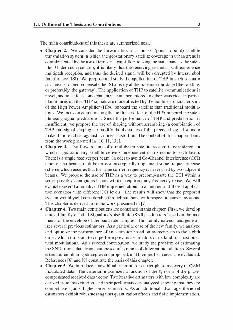
The basic setup of a Tomlinson-Harashima (TH) precoder is shown in Figure 2.2.
Here, the transfer function H(z) is considered to be causal and minimum-phase, with
h0 = 1 (monic polynomial). Again, the channel inversion is implemented via a nega-
tive feedback structure, but now a modulo device is inserted into the feedforward branch,
which introduces a nonlinearity in the precoding operation. In order to recover the (noisy)
original symbols, the receiver must apply again the same modulo operation performed at
the receiver. The fact that THP operates at the transmitter automatically prevents error
propagation. As additional advantage, THP can be straightforwardly used in conjunction
with current coding schemes (such as LDPC codes [90]). Similarly to linear preequaliza-
tion, the channel transfer function needs to be known at the transmitter.
The operational principle of THP lies upon lattice theory: the use of modulo arithmetic
allows us to represent one symbol not only by that lying in the original constellation set,
10 Chapter 2. Application of THP to Point-to-Point Satellite Communications
Figure 2.2: System using Zero-Forcing Tomlinson-Harashima precoding
but also by its correspondents in other (modulo-congruent) constellation replicas, as long
as these replicas are distributed according to a well-constructed lattice. To illustrate how
THP works, consider the signals an, fn (the feedback signal corresponding to the ISI), ynand zn from Figure 2.2. We have
fn =
p−1∑
k=1
hk xn−k (2.1)
xn = MOD∆ (an − fn) (2.2)
yn =
p−1∑
k=0
hk xn−k + wn = xn + fn + wn (2.3)
zn = MOD∆ (yn) = MOD∆ (xn + fn + wn)
= MOD∆ (MOD∆ (an − fn) + fn + wn) = MOD∆ (an + wn) . (2.4)
Therefore, in a noiseless case (wn = 0) we have that zn = an.
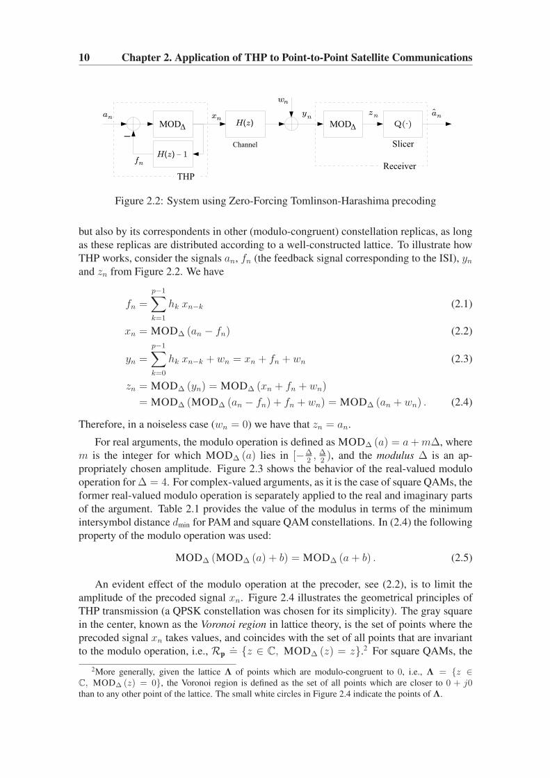
For real arguments, the modulo operation is defined as MOD∆ (a) = a+m∆, where
m is the integer for which MOD∆ (a) lies in [−∆2, ∆2), and the modulus ∆ is an ap-
propriately chosen amplitude. Figure 2.3 shows the behavior of the real-valued modulo
operation for ∆ = 4. For complex-valued arguments, as it is the case of square QAMs, the
former real-valued modulo operation is separately applied to the real and imaginary parts
of the argument. Table 2.1 provides the value of the modulus in terms of the minimum
intersymbol distance dmin for PAM and square QAM constellations. In (2.4) the following
property of the modulo operation was used:
MOD∆ (MOD∆ (a) + b) = MOD∆ (a+ b) . (2.5)
An evident effect of the modulo operation at the precoder, see (2.2), is to limit the
amplitude of the precoded signal xn. Figure 2.4 illustrates the geometrical principles of
THP transmission (a QPSK constellation was chosen for its simplicity). The gray square
in the center, known as the Voronoi region in lattice theory, is the set of points where the
precoded signal xn takes values, and coincides with the set of all points that are invariant
to the modulo operation, i.e., Rp.= {z ∈ C, MOD∆ (z) = z}.2 For square QAMs, the
2More generally, given the lattice Λ of points which are modulo-congruent to 0, i.e., Λ = {z ∈C, MOD∆ (z) = 0}, the Voronoi region is defined as the set of all points which are closer to 0 + j0than to any other point of the lattice. The small white circles in Figure 2.4 indicate the points of Λ.

2.2. Theoretical Background 11
Figure 2.3: MOD∆ (x) for real-valued x and ∆ = 4.
Table 2.1: Definitions and corresponding modulus ∆ for PAM and square QAM constel-
lations in terms of their minimum intersymbol distance dmin.
Constellation Symbols Modulus
M -PAM, M = 2q, q ∈ N A ={
±2i− 12 dmin, i = 1, 2, . . . , M2
}
∆ = M dmin
M -QAM, M = 22q, q ∈ N A = {aI + jaQ, with aI, aQ ∈ B}, where ∆ =√Mdmin
B =
{
±2i− 12 dmin, i = 1, 2, . . . ,
√M2
}
Voronoi region coincides with the half-open square given by Rp = {zI + jzQ,−∆2≤ zI <
∆2, −∆
2≤ zQ < ∆
2}, as shown in Figure 2.4. After transmission of xn, the channel adds
the ISI fn, and the signal at the receiver is a combination of the precoded symbol, ISI
and noise, see (2.3). Disregarding the noise contribution, the noiseless received symbol
xn + fn will always fall in a point which is congruent to an under MOD∆ (·) (such points
are marked in Figure 2.4 as the darkest points of each QPSK replica). Therefore, as
indicated in (2.4), THP allows to receive some modulo-congruent perturbation which will
be automatically removed by the modulo operation at the receiver thanks to property (2.5).
This allows to transmit the smallest (in magnitude) modulo-congruent difference between
the desired symbol and the existing ISI, i.e., xn.
In the light of the previous explanation it is not difficult to establish a similarity be-
tween the way THP works and the DPC principle mentioned in the introductory section
of this chapter. The DPC principle states that the most efficient way to counteract an addi-
tive interference known by the transmitter is to adapt the transmitted signal to the existing
interference, rather than the more “canonical” approach of precanceling the interference.
In the case of THP, the “canonical” approach would be represented by linear precoding,
which suffers from a power penalty, and therefore is inefficient. Instead, the modulo de-
vice of the TH precoder automatically selects the transmitted signal with the minimum
amplitude that ensures the correct reception (of a modulo-congruent replica) of the origi-
nal symbols. Hence, the transmitter takes advantage of the interference to efficiently use
the available transmit power, as the DPC principle teaches.

12 Chapter 2. Application of THP to Point-to-Point Satellite Communications
Figure 2.4: Example of transmission of a QPSK symbol using THP.
À The original QPSK symbol an is the darkest circle within the Voronoi region Rp (gray
square).
Á The transmitter subtracts the known ISI fn from an.
 Then the result an − fn is modulo-reduced yielding the precoded symbol xn to be
transmitted.
à At the receiver, the channel has added the ISI, so that (in absence of noise) the received
symbol xn + fn is a modulo-congruent replica of an.
Ä Finally, the modulo operation at the receiver reduces xn + fn to the Voronoi region
yielding an, as desired.

2.2. Theoretical Background 13
Figure 2.5: Linear equivalent model for THP.
Linearized THP model As already mentioned, the presence of the modulo operation
renders the whole transmission model nonlinear, and this prevents the application of the
results from the well-established theory of linear systems. However, it is possible to find
a linearized equivalent version of the THP procedure, which will be useful later on. As
shown in Figure 2.5, some new ad-hoc signals are needed, namely dn (the precoding
sequence), vn (the effective data sequence, which is a noise-free version of the received
signal yn), and dn. The following definitions and relationships will be useful:
dn.= (an − fn)− MOD∆ (an − fn) (2.6)
vn.= an + dn (2.7)
= xn + fn =
p−1∑
k=0
hkxn−k (2.8)
yn = vn + wn (2.9)
dn.= yn − zn = yn − MOD∆ (yn) (2.10)
From (2.6) and (2.10), it is clear that dn and dn take values on the set of points that are
modulo-congruent to 0 under the modulo operation MOD∆ (·). (these points, which are
marked as small white circles in Figure 2.4, constitute a lattice).
Description of the involved signals We summarize next the statistical features of the
different discrete sequences involved in THP transmission, assuming that the channel
introduces a sufficiently large amount of ISI [59]:
• an: independent and identically distributed (i.i.d.) symbols equiprobably drawn
from a square QAM constellation A with M elements (Pulse Amplitude Modulation
(PAM) signaling will not be further considered), with minimum intersymbol dis-
tance dmin. Therefore, its Probability Density Function (pdf) is a discrete uni-
form distribution taking values at the symbol locations. The average energy of a
square QAM (for which M = 22q, with q ∈ N) is given by σ2a
.= E {|an|2} =
d2min(M − 1)/6.
• dn and dn: from (2.6) and (2.10) it is clear that both sequences take values at points
which are congruent to 0 under the modulo operation MOD∆ (·). In fact, these
points constitute the precoding lattice Λ. In the case of a square QAM the lattice is
given by
Λ = {dI + jdQ, with dI = m∆, dQ = n∆, m, n ∈ Z}.

14 Chapter 2. Application of THP to Point-to-Point Satellite Communications
The small white circles in Figure 2.4 indicate the points of Λ.
• vn: the effective data sequence follows a discrete Gaussian pdf, which takes values
at the expanded signal set with a Gaussian decay.3 For square QAMs the support
set is given by [112] V = {vI +j vQ with dI = mdmin/2, dQ = ndmin/2, m, n ∈ Z},
and the associated probabilities are given by
f(v) = c · exp
(
− |v|2∆2η
)
, for v ∈ V
where c > 0 is a normalization constant and η > 0 is the so-called granularity
parameter. For a fixed ∆, η accounts for the span of f(v) (large η causes long
tails). In general, η grows with the amount of ISI introduced by the channel.
• xn: the precoded sequence is an almost i.i.d. sequence, uniformly distributed within
the region delimited by the output of the modulo operation. The modulo operation
has thus a whitening effect on its output. The average energy of the sequence is
given by
σ2x.= E
{|xn|2
}= ∆2/6 (2.11)
for square regions of side ∆. For square QAMs, this variance can be written as
σ2x = M d2min/6.
THP presents an SNR penalty with respect to normal QAM transmission, due to a
slight increase in the transmitted power. The so-called precoding loss is defined as [59]
γ2p.=
σ2x
σ2a
=E {|xn|2}E {|an|2}
. (2.12)
Under sufficiently strong ISI conditions, the precoding loss is a function of the modulus ∆and the original constellation. In particular, for QAM signaling the precoding loss reduces
to γ2p = M/(M − 1), which indicates that the loss becomes negligible as the constellation
size increases (i.e., for high-rate transmission). Table 2.2 illustrates this fact.
Table 2.2: Dependence of the precoding loss with the square QAM constellation size.
QAM size γ2p γ2
p
M (linear units) (dB)
4 (QPSK) 1.333 1.2516 1.067 0.2864 1.016 0.06256 1.004 0.021024 1.001 0.00
3Such distribution is related to the Gaussian distribution of the ISI, fk, although a formal justification
of the discrete Gaussian nature of vn is complicated due to the nonlinear effect of the modulo operation.
Instead, such pdf can be easily checked using simulations.

2.2. Theoretical Background 15
2.2.1.3 ZF-THP and MMSE-THP
So far we have only considered the use of THP designed according to the ZF criterion. The
goal of the ZF approach to equalization, which is based upon the inversion of the channel
transfer function, is to completely remove the ISI introduced by the channel. As mentioned
in Section 2.2.1.1, the application of this criterion in linear equalization may incur noise
enhancement when there are spectral notches in the channel frequency response, but this
problem is avoided by nonlinear techniques such as DFE and THP. An alternative solution
is to use the Minimum Mean Square Error (MMSE) criterion (see e.g. [59]), which avoids
the noise enhancement problem in linear equalization since it considers the noise variance
in addition to the channel transfer function (both must be known in order to design the
equalizer). In contrast to the ZF criterion, the MMSE criterion admits some residual
interference after correction which helps prevent noise enhancement. Generally speaking,
MMSE equalization offers better results than ZF equalization at low SNRs, whereas both
criteria tend to converge asymptotically as the SNR grows (they coincide in the limit).
Although THP designed according to the ZF criterion (ZF-THP) does not suffer from
noise enhancement, it turns out that the MMSE approach offers performance improve-
ments over the ZF approach at low SNRs, as it does for linear equalization. Therefore,
both approaches (ZF-THP and MMSE-THP) will be considered in this chapter. The dif-
ference between both approaches lies in how the filters are computed. We refer to Ap-
pendix 2.A for the details on the actual filter computation.
2.2.2 Combining THP and Signal Shaping
2.2.2.1 Introduction to Signal Shaping
Many communication systems typically work under quite demanding conditions in terms
of power or interference limitations. In such scenarios, it is crucial to achieve good SNR
efficiency in the transmission. Traditionally, SNR efficiency has been pursued by means
of coding. However, it is well known today that the total improvement in SNR efficiency
can be separated into two contributions: coding gain and shaping gain [65].4 Whereas
coding seeks to minimize the probability of error in the transmission, the goal of signal
shaping is to find the transmitted signal that achieves the desired performance with a
minimum cost. Typically, this cost is the average transmit power, which leads to energy-
efficient transmissions, although other cost functions can be considered. In all cases,
signal shaping modifies the mapping between the source bits and the transmitted symbols,
so as to accommodate the pdf of the symbols to achieve the desired goal.
The shaping gain is defined as the transmit power reduction achieved by signal shap-
ing with respect to the corresponding conventional scheme in which equiprobable signal-
ing is used. In terms of shaping gain, it is desirable that the boundary of the transmitted
signal be as close as possible to a circle (in two dimensions), or in general to an N -sphere
4This assertion is valid at high data rates, when dense constellations are used. For low rates both contri-
butions are not fully separable.

16 Chapter 2. Application of THP to Point-to-Point Satellite Communications
(the generalization of the sphere in N th-dimensional space, useful when more dimen-
sions are used in the shaping operation).5 In general, moving to higher dimensions allows
to achieve larger shaping gains [62, 65], although there is an upper bound: the ultimate
shaping gain, which amounts to πe/6 (or 1.53 dB).
Generally speaking, shaping gains cannot be achieved without negatively affecting
other parameters of the transmitted signal. In particular, larger peak energies must be
transmitted, and some degree of redundancy must be added to the transmitted signal
(which is accommodated by increasing the number of symbols in the constellation) in
exchange for the average energy reduction. We will use the following measures to quan-
tify such effects:
• Peak-to-Average Energy Ratio (PAR), defined as the ratio of the peak energy in the
constellation to the average energy;
• Constellation Expansion Ratio (CER), defined as the ratio between the size of the
(augmented) constellation used for shaping and the baseline equiprobable constel-
lation. It is always verified that CER ≥ 1.
Signal shaping can be implemented by several means. We cite here the most represen-
tative ones:
• Shell Mapping. This technique is related to a kind of fixed-rate vector quantizer
used in source coding. Detailed descriptions can be found in [104] and [59, chapter
4].
• Trellis Shaping. In this technique, the transmitted sequence is found using a trellis
decoder. The trellis is built according to a given code (the shaping code), and the
decoder must minimize the aggregate cost (typically the average energy) of the
transmitted sequence. Trellis shaping is well described in the original source [64],
as well as in [59, chapter 4].
2.2.2.2 Shaping for THP: Shaping Without Scrambling
Unfortunately, THP is not well suited for direct combination with signal shaping, because
the shape of the signal at the output of the modulo device typically differs considerably
from that of the signal at its input. Instead, shaping can only be applied to THP sig-
nals when both operations are performed jointly. This can be achieved by means of two
techniques: trellis precoding and shaping without scrambling. Both schemes are closely
related: similarly to trellis shaping, both use a Viterbi decoder at the transmitter to select
the sequence with minimum weight. However, shaping without scrambling presents some
advantages over trellis precoding, one of which is that it is fully compatible with THP
from the receiver point of view. For this we will exclusively consider shaping without
scrambling for our proposed system, and no details will be given here on trellis precod-
ing. The reader is referred to the original work [57], and to [59, chapter 5] for details on
that technique.
5The circle (or N -sphere) is the geometrical shape of least average energy for a given volume in two
dimensions (N dimensions).

2.2. Theoretical Background 17
As mentioned above, signal shaping requires that some redundancy be added to the
transmitted signal. In shaping without scrambling this is implicitly done by enlarging the
support range of the constellation (i.e., the region delimited by the modulo operation at
the transmitter) to some extent, but keeping the same modulo operation at the receiver as
in plain THP. If, in addition, the same minimum intersymbol distance dmin used in THP
is maintained, then the enlarged support range for transmission translates into the use of
extra symbols which lie outside the boundaries of the original constellation.
The reason why this works is the following. In plain THP, the modulo operation tightly
encloses the boundaries of the original constellation. Therefore, recalling the linearized
model of Figure 2.5, the precoding sequence dn is uniquely determined by the modulo op-
eration, as indicated by (2.6). This sequence yields a precoded sequence xn that presents
a uniform pdf within the support range of the modulo operation, as we have seen. Now, if
we allow the use of a larger support range, say by an integer factor K (thus CER = K),
but keeping the same modulo operation as in THP at the receiver, then the choice of the
precoding sequence is not unique: there are K possible values for dn at each instant that
will yield K different precoded symbols xn within the enlarged support range, and all of
them will produce the same output after the modulo operation in the receiver. It is this
redundancy that shaping takes advantage of: the actual sequence is adequately chosen to
meet the desired requirement (e.g. reduce the average transmitted power). Interestingly,
it can be shown [59, chapter 4] that CER = 2 (one bit redundancy) is sufficient to achieve
most of the available shaping gain.
In Figure 2.6 we display the constellations and support regions used when applying
shaping without scrambling in two dimensions with one bit redundancy to a 16-QAM
constellation. Note that the support region for shaping (and therefore the modulo oper-
ation at the transmitter) remains square, but is rotated 45◦. Note also that the expanded
constellation shown in Figure 2.6c (the union of a 16-QAM and a shifted version, with
shift λ) is only one possibility. The actual region of the transmitted sequence xn is even-
tually determined by the modulo operation corresponding to the support region in 2.6d,
regardless of the chosen expanded constellation, as long as the latter is well built.
The block diagram of a system using shaping without scrambling is shown in Fig-
ure 2.7. The receiver is identical to that of a THP system. The transmitter operates as
follows. Recalling that one bit shaping is enough to achieve most of the available shaping
gain, a constellation with twice the number of symbols of the original constellation (CER
= 2) will be used for shaping, as shown in Figure 2.6c. With this, the role of the sequence
selector in Figure 2.7 is to decide whether to precode the original constellation symbol anor its equivalent in the expanded replica, which we denote as an + λ. Note that, as seen
in Figure 2.6, the shift λ is modulo-congruent to 0 under the MOD∆ (·) operation. Thus,
the signal entering the precoding operation can be written as pn = an + bnλ, where bn is
a binary sequence taking the values 1 or 0 depending on whether the shift λ takes place
or not. The precoding operation is similar to that in plain THP, except for the modulo op-
eration, which must now match the new support region used for shaping. We will denote
this operation as MOD(s)√2∆
(·), where the superscript (s) differentiates it from the modulo
operation performed at the receiver (and in plain THP).
As already explained, the sequence selection reduces to a binary decision for each

18 Chapter 2. Application of THP to Point-to-Point Satellite Communications
(a) (b)
(c) (d)
Figure 2.6: Constellations and support regions for shaping without scrambling with CER
= 2: (a) original constellation, 16-QAM; (b) support region in THP; (c) possible expanded
constellation with 32 symbols; (d) support region for shaping.
transmitted symbol (represented by the signal bn). This selection is carried out by a Viterbi
decoder. The reader is referred to the classical tutorial [63] for the basics of Viterbi de-
coding, which will be omitted here. Rather, we will focus on the key elements used in
shaping. The Viterbi decoder operates on a trellis, which is built upon a virtual convolu-
tional scrambler.6 The choice of the actual scrambler used is not important, as long as the
number of states is sufficient, as shown in [59, chapter 5]. Hence, a possible choice for
the generator polynomial is (D-transform notation is used):
S(D) = 1⊕D ⊕Ds (2.13)
where s ∈ N allows to control the number of states of the scrambler (2s states). The
Viterbi decoder is designed to minimize a given metric which is accumulated along the
surviving sequences arriving at each of the 2s states of the trellis. For example, in classical
shaping, where the goal is to minimize the average transmit power, the branch metric used
by the Viterbi decoder must account for the energy of the transmitted symbol associated
6A convolutional scrambler can be seen as a convolutional code of rate 1/1. The scrambler is virtual
because it does not physically exist at the transmitter; it is simply an algebraic tool to obtain a trellis
representation which allows the use of Viterbi decoding for sequence selection.

2.2. Theoretical Background 19
(a)
(b)
Figure 2.7: Block diagram of shaping without scrambling: (a) transmitter side; (b) re-
ceiver side.
to each state transition. The metric for state S reads
µn =∣∣x(S,b)
n
∣∣2=∣∣∣MOD
(s)√2∆
(an + bnλ− f (S)
n
)∣∣∣
2
(2.14)
where x(S,b)n is the transmitted symbol associated to the transition leaving state S with
the binary value bn, and f(S)n
.=∑p
k=1 hkx(S)n−k is the ISI corresponding to the candidate
sequence, which depends on the p (candidates to) past symbols x(S)n−k. Later in Section 2.4
we will propose other more elaborate metrics which seek other simultaneous goals such
as peak-to-average ratio reduction.
2.2.3 Signal Predistortion
In a standard communication system, waveforms are generated at the transmitter at low
levels and need to be amplified before they are radiated in order to close the link bud-
get, i.e., in order to ensure they reach the receiver with at least the minimum required
SNR. The amplification step is achieved by means of HPAs. These amplifiers are often
an expensive part of the communication chain, both in terms of device cost and power
consumption. Therefore, efficiency in HPA operation is a must in the design of most cur-
rent transmitters. Satellite communications, where HPAs must typically yield large output

20 Chapter 2. Application of THP to Point-to-Point Satellite Communications
powers to compensate large free space losses, provide an extreme example of a communi-
cation system with demanding requirements in terms of power efficiency. However, there
is a negative effect associated to high amplification: HPAs introduce nonlinear distor-
tion in the amplified signal when they are forced to work close to their saturation points.
Therefore a trade-off is established between the desire to achieve larger signal power and
the undesired HPA distortion. Next we provide a brief overview of the distortion models
and the compensation techniques existing in the literature.
2.2.3.1 Nonlinear Effect of the HPA
Accurately modeling the effect of the HPA allows the design of appropriate compensation
methods. Different approaches exist to address the characterization of the HPA nonlinear-
ities, depending on a number of factors such as the type of amplifier, or whether memory
is included in the model. In this work we consider only memoryless models (Saleh and
Rapp), which are the simplest to compensate. We briefly describe them next, including
for completeness also the most representative models with memory found in the literature.
Saleh’s model This is a memoryless model, originally introduced in [139] to model the
effect of Traveling Wave Tube Amplifiers (TWTAs). The nonlinear distortion depends
exclusively on the instantaneous envelope of the input signal. Let x(t) = r(t) cos(2πf0t+φ(t)) be the band-pass input signal, where r(t) is the real-valued instantaneous envelope,
f0 the carrier frequency, and φ(t) the instantaneous phase. According to Saleh, the HPA
output is modeled as
y(t) = A [r(t)] cos (2πf0t+ φ(t) + Φ[r(t)]) (2.15)
where A[·] and Φ[·] are, respectively, the AM/AM and AM/PM characteristics of the non-
linearity, given by
A[r] =αa r
βa r2 + 1(linear units) (2.16)
Φ[r] =αp r
2
βp r2 + 1(rad). (2.17)
The parameters αa, βa, αp, βp are chosen to match the characteristics of the particular
amplifier, originally obtained through measurement.
If more accuracy is desired, Saleh’s model can be straightforwardly extended by con-
sidering the ratio of full second-order polynomials both for the AM/AM and AM/PM
characteristics:
A[r] =αa,2 r
2 + αa,1 r + αa,0
βa,2 r2 + βa,1 r + 1(linear units) (2.18)
Φ[r] =αp,2 r
2 + αp,1 r + αp,0
βp,2 r2 + βp,1 r + 1(rad). (2.19)
We will refer to (2.18)–(2.19) as the generalized Saleh’s model.

2.2. Theoretical Background 21
Rapp’s model This is also a memoryless model, first presented in [133], which de-
scribes the effect of Solid State Power Amplifiers (SSPAs). This model is simpler than
the Saleh’s model in that only AM/AM conversion is considered, since the amplifier is
assumed to introduced no phase distortion [i.e., Φ[r] = 0 in (2.15)]. The AM/AM charac-
teristic under Rapp’s model is given by
A[r] =v r
[
1 +(
v rr0
)2p]1/(2p)
(linear units) (2.20)
where the parameters v, r0 and p take positive values and correspond to, respectively,
the small signal gain, the limiting amplitude, and the smoothness factor controlling the
transition from the linear region to the saturation region of the amplifier.
Models with memory Saleh’s and Rapp’s models are examples of memoryless models.
If memory is to be accounted for in the model (e.g., in applications with large bandwidth
such as W-CDMA or W-OFDM), then several approaches can be used. We cite next the
most representative ones.
1. Wiener model. This model consists of the concatenation of a linear filter g(t) and a
nonlinear memoryless function f(·). The output signal can be written as
y(t) = f(x(t) ∗ g(t)). (2.21)
2. Hammerstein model. If the order of the blocks in the Wiener model is switched (i.e.,
memoryless nonlinearity first, then linear filter), then we have a Hammerstein model.
Its output signal can be written as
y(t) = f(x(t)) ∗ g(t). (2.22)
3. Memory polynomial. Memory polynomials are another simple way to include mem-
ory effects in the model. The baseband version of the output signal is given by [50,
103]
yn =M∑
m=0
xn−m
pm∑
k=1
bm,k|xn−m|k−1 (2.23)
where bm,k are the coefficients of the model.
4. Volterra series model. The Volterra series is the most general nonlinear model, and
comprises all previous models as particular cases. Its discrete-time expression is given
by [22]
yn =∞∑
k=1
∑
n1
· · ·∑
n2k−1
H(2k−1)(n1, . . . , n2k−1)k∏
i=1
xn−ni
2k−1∏
i=k+1
x∗n−ni
(2.24)
where H(p)(n1, . . . , np) is known as the p-th order Volterra kernel (for p odd).

22 Chapter 2. Application of THP to Point-to-Point Satellite Communications
2.2.3.2 Compensation Techniques
The compensation of the HPA-induced nonlinearity can be seen as a linearization prob-
lem: the ultimate goal is to remove the nonlinear contribution of the HPA. Such task is not
fully achievable due to non-invertibility of the nonlinearity, although partial linearization
can be achieved in general in a given range of the input-output characteristic, or at given
sampling instants.
Several techniques have been reported in the literature as means to mitigate the non-
linear distortion introduced by the HPA:
• Back-off. The most straightforward choice is to back off from saturation. The Input
Back-Off (IBO) is a useful system parameter defined as the ratio of the saturation
power Psat,in to the average input power Pin, i.e.,
IBO.=
Psat,in
Pin
. (2.25)
Large IBOs drive the working point into the HPA’s linear region (the so-called small
signal characteristic), thus preventing nonlinear effects. However this solution
comes at the expense of (i) a reduced Direct Current to Radio Frequency (DC/RF)
conversion efficiency, and (ii) a reduction of the available RF output power, which
makes the link budget fulfillment difficult. This latter unwanted effect is measured
by the Output Back-Off (OBO), which relates the maximum output power Pmax,out
to the average output power Pout:
OBO.=
Pmax,out
Pout
. (2.26)
In practice, some degree of IBO is typically used in combination with any of the
compensation techniques described next. A trade-off must be established between
the desired nonlinear interference mitigation and the undesired OBO.
• Postdistortion. A second possibility is the use of mitigation techniques at the re-
ceiver side. This can be efficiently achieved by using nonlinear equalizers [21], or
by using maximum-likelihood sequence detection [119], which achieves optimum
performance at high computational cost. The drawbacks of postdistortion are the
augmented complexity of the receiver and the impossibility to prevent undesirable
adjacent channel interference in the transmitted signal.
• Predistortion. In order to solve these latter issues, compensation can be introduced
at the transmitter, before the HPA stage. In predistortion, the signal fed into the
HPA has previously undergone a certain nonlinear function designed to yield a
distortion-free signal at the HPA output (at least to some extent). Predistortion can
be performed in two ways, depending on which signal it is applied to:
– Data predistortion operates on the mapping between the binary information
and the effective constellation points, prior to the conversion to waveform via
the transmit filter. The underlying principle is to modify the location of the
original constellation points in such a way that the effect of the HPA returns
them close to their original location. Since this operation is performed before

2.3. Point-to-Point Scenario Description 23
the pulse shaping filter, the effects of this filter and the receive filter must be
taken into account for the compensation.
– Fractional predistortion (also waveform or signal predistortion) is performed
after the pulse shaping filter, thus needing to compensate for the HPA nonlin-
earity only. Waveform predistorters can be implemented both in analog and
in digital form. In the analog case, they operate in radio frequency (RF) (or
possibly intermediate frequency (IF)) and are typically made up of discrete
components. In the digital case, they typically operate in baseband at over-
sampled rate. Digital predistorters have the advantage that they can be easily
made adaptive to track system characteristics changes as a consequence of a
variation in the signal characteristics (i.e., the pdf) or in the power amplifier
characteristics, as a function of temperature, ageing or bias fluctuations.
For the aforementioned advantages, digital fractional predistortion combined with input
back-off will be the compensation technique considered in this work.
2.3 Point-to-Point Scenario Description
Before giving the details of the proposed systems, we will provide the description of the
scenario under which our solutions will be evaluated. We consider the forward link of a
Geostationary Earth Orbit (GEO) satellite system such as that depicted in Figure 2.8. A
fixed or nomadic ground-based terminal is located in an urban environment, and receives
a data stream from the GEO satellite and one or several IMRs. The data stream, which
is specifically intended to that given terminal (point-to-point or unicast transmission), is
generated at a ground-based gateway station. The gateway sends the data stream to the
satellite using the feeder link. Since it is likely that the satellite system must deliver some
other content (e.g., other streams toward different users, broadcast TV service, etc), the
gateway will be required to perform some kind of multiplexing (typically in frequency
and polarization) of the signals before they are amplified and sent through the feeder link.
The satellite will then perform the appropriate demultiplexing and frequency conversions
to the signals before being transmitted to ground. The IMRs act as repeaters, i.e., they
operate on the same band and use the same modulation as the direct signal coming from
the satellite).
The following assumptions are made regarding the elements of the transmission chain.
As2.1) Transparent IF and RF conversions. All frequency conversions in the chain are
ideal, i.e., they do not introduce any degradation in the transmitted signals.
As2.2) Transparent (de)multiplexing. The multiplexing at the gateway and the demul-
tiplexing onboard do not alter the transmitted signals.
As2.3) Transparent repeaters. The IMRs act as ideal relays, i.e., they introduce neither
any delay nor any degradation in the repeated signal.
As2.4) No cochannel interference. The signal received at the ground terminal is not af-
fected by signals corresponding to other services or other possible receivers. This
amounts to assuming some kind of frequency multiplexing in the data services
offered by the satellite.

24 Chapter 2. Application of THP to Point-to-Point Satellite Communications
Feeder link
Gateway
Receiver
LOS
path
IMR
IMR
IMR
Reflected path
Urban area
THP
Figure 2.8: Point-to-point transmission scenario considered, in which THP is performed
at the gateway.
As2.5) Perfect timing and carrier recovery. The receiver is assumed to implement
sufficiently accurate timing, phase and frequency acquisition schemes, so that they
do not have any impact in the received signal.
As2.6) Nonlinear distortion. The HPAs at the gateway and at the IMRs are assumed to
operate under linear conditions thanks to, e.g., a generous back-off margin [39].
Thus, the only source of nonlinear distortion is the HPA onboard the satellite,
whose characteristic will be known to the predistortion stage.
As2.7) Perfect CSI knowledge at the transmitter. The Channel State Information
(CSI), i.e., the channel response of the forward link, is assumed to have a suffi-
ciently slow variation (quasi-static channel) so that some channel estimation pro-
cedure can perfectly estimate and track the channel state at any moment. If such
estimation is performed at the receiver, the existence of an ideal return channel is
furthermore assumed so that the estimated CSI can be accurately passed back to
the transmitter. Perfect CSI knowledge is required for the proper application of
THP transmission as presented in Section 2.2. We refer to Appendix 3.E where
we discuss the effects of inaccuracies in the estimated channel impulse response.
With the former assumptions, gateway and satellite act as a single transmitting unit
from the receiver’s point of view, and the signal received by the terminal will most likely
be corrupted by ISI due to the multiple signals (and their possible reflections) coming
from the satellite and the IMRs. In addition, such signal will suffer from nonlinear dis-
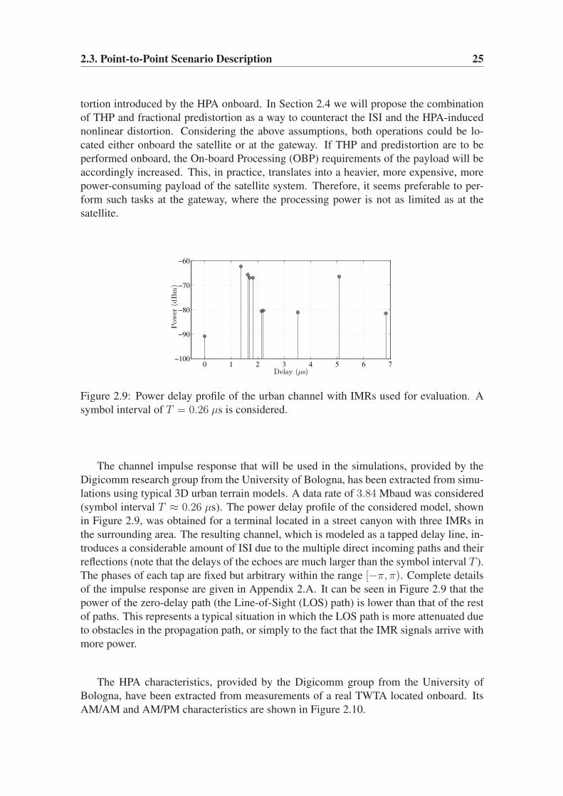
2.3. Point-to-Point Scenario Description 25
tortion introduced by the HPA onboard. In Section 2.4 we will propose the combination
of THP and fractional predistortion as a way to counteract the ISI and the HPA-induced
nonlinear distortion. Considering the above assumptions, both operations could be lo-
cated either onboard the satellite or at the gateway. If THP and predistortion are to be
performed onboard, the On-board Processing (OBP) requirements of the payload will be
accordingly increased. This, in practice, translates into a heavier, more expensive, more
power-consuming payload of the satellite system. Therefore, it seems preferable to per-
form such tasks at the gateway, where the processing power is not as limited as at the
satellite.
0 1 2 3 4 5 6 7−100
−90
−80
−70
−60
Delay (µs)
Pow
er(d
Bm
)
Figure 2.9: Power delay profile of the urban channel with IMRs used for evaluation. A
symbol interval of T = 0.26 µs is considered.
The channel impulse response that will be used in the simulations, provided by the
Digicomm research group from the University of Bologna, has been extracted from simu-
lations using typical 3D urban terrain models. A data rate of 3.84 Mbaud was considered
(symbol interval T ≈ 0.26 µs). The power delay profile of the considered model, shown
in Figure 2.9, was obtained for a terminal located in a street canyon with three IMRs in
the surrounding area. The resulting channel, which is modeled as a tapped delay line, in-
troduces a considerable amount of ISI due to the multiple direct incoming paths and their
reflections (note that the delays of the echoes are much larger than the symbol interval T ).
The phases of each tap are fixed but arbitrary within the range [−π, π). Complete details
of the impulse response are given in Appendix 2.A. It can be seen in Figure 2.9 that the
power of the zero-delay path (the Line-of-Sight (LOS) path) is lower than that of the rest
of paths. This represents a typical situation in which the LOS path is more attenuated due
to obstacles in the propagation path, or simply to the fact that the IMR signals arrive with
more power.
The HPA characteristics, provided by the Digicomm group from the University of
Bologna, have been extracted from measurements of a real TWTA located onboard. Its
AM/AM and AM/PM characteristics are shown in Figure 2.10.

26 Chapter 2. Application of THP to Point-to-Point Satellite Communications
−20 −15 −10 −5 0 5 10−15
−10
−5
0
IBO (dB)
OB
O(d
B)
Phase
(deg
)
0
10
20
30
40
50
60
AM/AM
AM/PM
Figure 2.10: AM/AM and AM/PM characteristics of the TWTA onboard used for evalua-
tion.
2.4 Proposed Schemes
2.4.1 Combined THP and Predistortion
We will study the combined performance of THP and fractional predistortion under un-
coded transmission. A reference system with fractional predistortion and DFE at the
receiver will be used for comparison.
The block diagram of the proposed system is shown in Figure 2.11. A bit sequence
is mapped onto QAM symbols, which are then precoded using the standard TH scheme
detailed in Section 2.2.1.2. The precoded symbols are converted to waveform by a pulse-
shaping filter, which we consider a Square Root Raised Cosine (SRRC) filter of roll-off
0.3. The oversampling factor within the waveform domain is set to 4. The waveform is
applied fractional predistortion before entering the HPA. The channel is a complex-valued
tapped delay line as described in Section 2.3, after which complex AWGN is added. The
receiver front end is a Whitened Matched Filter (WMF), which after baud rate sampling,
yields a signal affected by ISI and Additive White Gaussian Noise (AWGN). The re-
maining ISI is removed by the modulo operation at the receiver, and then a QAM slicer
produces an estimate of the transmitted symbol.
The reference system combining fractional predistortion and DFE is depicted in Fig-
ure 2.12. The only change with respect to our proposed system of Figure 2.11 is that the
TH precoder and the modulo operation at the receiver are substituted by a DFE.
In this section, perfect timing and carrier recovery is assumed. We refer to Ap-
pendix 2.B, where some considerations are given regarding the timing recovery problem
under THP transmission. Details on the computation of the filters involved in the system
are given in Appendix 2.A.
Fractional predistorter We consider a fractional predistorter implemented using a Look-
Up Table (LUT). The HPA characteristics provided in Section 2.3 (Figure 2.10), are ap-
proximated using the generalized Saleh’s model given by (2.18)–(2.19). The measured
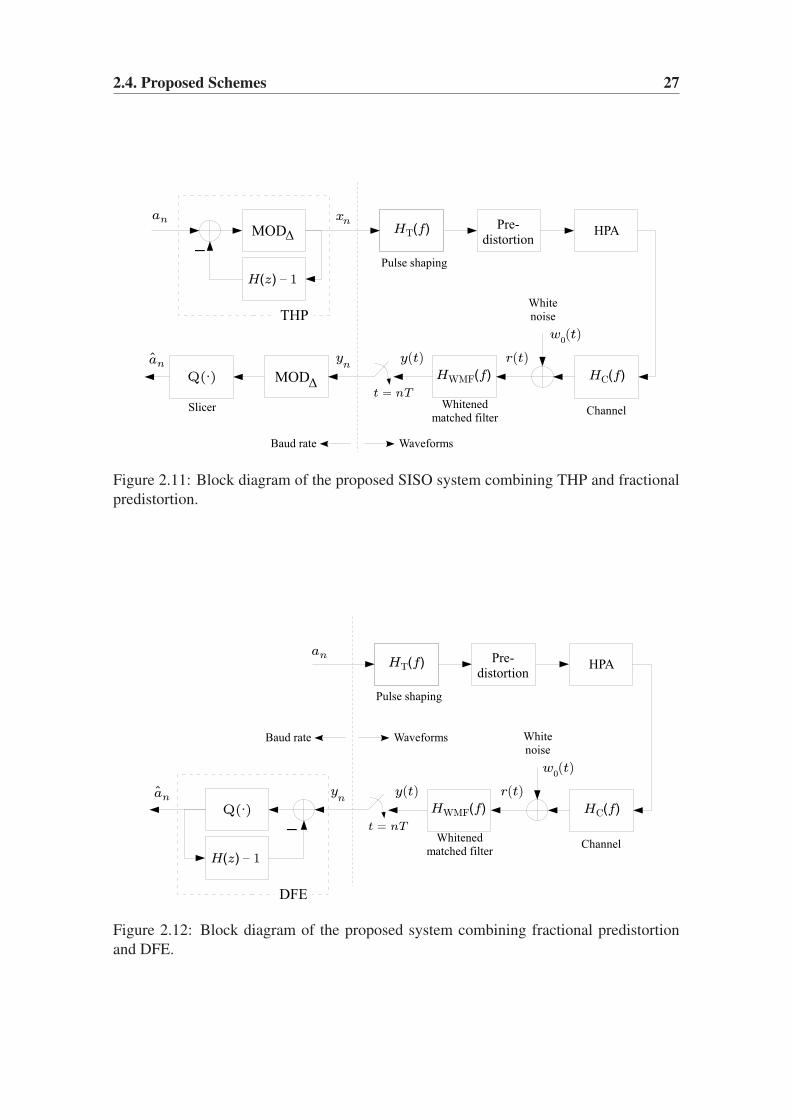
2.4. Proposed Schemes 27
Figure 2.11: Block diagram of the proposed SISO system combining THP and fractional
predistortion.
Figure 2.12: Block diagram of the proposed system combining fractional predistortion
and DFE.

28 Chapter 2. Application of THP to Point-to-Point Satellite Communications
Table 2.3: Parameters of the generalized Saleh’s model fitting of the HPA characteristics.
AM/AM αa,2 αa,1 αa,0 βa,2 βa,1
−0.0494 1.7564 0.0247 1.0393 −0.2649AM/PM αp,2 αp,1 αp,0 βp,2 βp,1
0.3182 0.43898 −0.0324 0.6150 −0.4681
HPA characteristics are approximated using nonlinear least squares fitting. The resulting
parameters are given in Table 2.3, and yield the result shown in Figure 2.13. The inverted
AM/AM and AM/PM characteristics are stored in a LUT with 1024 entries indexed by the
instantaneous signal power, as shown in Figure 2.14. LUT entries are uniformly spaced
along the input signal power range (linear in power indexing), and contain the complex
predistortion factors.
−20 −15 −10 −5 0 5 10−15
−10
−5
0
IBO (dB)
OB
O(d
B)
Phase
(deg
)
0
10
20
30
40
50
60
AM/AM measured
AM/AM fit
AM/PM measured
AM/PM fit
Figure 2.13: Approximation of the HPA AM/AM and AM/PM characteristics using the
generalized Saleh’s model.
Figure 2.14: Block diagram of the LUT-based fractional predistorter with power indexing.
2.4.2 Combined Shaping Without Scrambling and Predistortion
As a way to improve the performance of the system with THP and predistortion proposed
in the previous section, we consider here the combination of shaping without scrambling

2.4. Proposed Schemes 29
and predistortion. As explained in Section 2.2.2, shaping without scrambling can yield a
precoded signal with improved characteristics over plain THP.
As mentioned in Section 2.2.1.2, assuming that the channel introduces a sufficiently
large amount of ISI, the output signal xk of the TH precoder can be considered to follow
a uniform distribution within the region delimited by the modulo operation (which is a
square if square QAM constellations are considered). Such signal exhibits a large dynamic
range, which after the SRRC filter translates into a waveform with a very disperse ampli-
tude distribution, which is certainly undesirable considering the nonlinear amplification
stage at the transmitter. In general, even if predistortion is applied, it is convenient that the
distribution of amplitudes at the HPA input be as concentrated as possible so as to reduce
the amount of nonlinear distortion. This is the reason why Constant Modulus (CM) con-
stellations such as Phase Shift Keying (PSK) have been traditionally preferred for satellite
communications to multilevel constellations such as QAM.
In this context, the use of shaping without scrambling can reduce the impact of the
HPA by modifying the signal distribution at its input. Figure 2.15 displays the block
diagram of the considered system with shaping without scrambling and predistortion.
The blocks performing the shaping operation and the TH decoding operate as explained
in Section 2.2.2.2 (see Figure 2.7). The generator polynomial used in the Viterbi decoder
Figure 2.15: Block diagram of the proposed system combining shaping without scram-
bling and fractional predistortion.
is S(D) = 1⊕D⊕D4, and thus is a member of the family (2.13) with s = 4. The decoder
operates therefore on 24 = 16 states.
h
Metric Selection for Shaping Without Scrambling The choice of the metric used by
the Viterbi decoder will determine the characteristics of the statistical distribution of the
shaped signal. The ultimate design criterion of the shaping stage should be the overall im-
provement of the system in terms of, e.g., Bit Error Ratio (BER). However, the complexity

30 Chapter 2. Application of THP to Point-to-Point Satellite Communications
of the transmission chain, especially the inherent nonlinearity of the shaping, precoding,
amplification and TH decoding stages, makes it difficult to map such ultimate goal onto a
corresponding metric for the trellis precoder. Instead, one must resort to heuristic criteria
for the selection of a shaping metric.
As a starting point we will consider the standard metric (2.14) which accounts for the
instantaneous energy of the precoder output. As mentioned in Section 2.2.2.2, minimiza-
tion of this metric yields the precoded sequence with minimum average energy. However
the reduction in average energy (the shaping gain) comes at the expense of an increase in
the Peak-to-Average Power Ratio (PAR) of the precoded sequence, which is undesirable
considering the nonlinear amplification stage (large peak values would either incur large
nonlinear distortion or require a large IBO to prevent such distortion, both undesirable
effects). Exploiting the flexibility in the metric design allowed by the Viterbi decoder, we
will next propose a number of alternative metrics which, heuristically, try to improve the
overall performance.
1. Minimization of average energy. This is the metric (2.14), which we reproduce here
for convenience
µ(1)n =
∣∣x(S,b)
n
∣∣2=∣∣∣MOD
(s)√2∆
(an + bnλ− f (S)
n
)∣∣∣
2
. (2.27)
Recall that x(S,b)n is the precoded symbol associated to the trellis transition leaving
state S with the binary value bn, and f(S)n
.=∑p
k=1 hkx(S)n−k is the ISI corresponding to
the candidate sequence, which depends on the p past symbols x(S)n−1, . . . , x
(S)n−p. Min-
imization of this metric yields a precoded sequence with minimum average energy,
but large PAR.
2. Joint minimization of average energy and Peak-to-Average Energy Ratio. If instead
of the quadratic order of the metric (2.27) we use a generic power q, we introduce
one degree of freedom in the metric design that can be exploited. The metric to be
minimized under this criterion is given by
µ(2)n =
∣∣x(S,b)
n
∣∣q. (2.28)
Intuitively, if q > 2 is chosen, the optimal reduction of energy will not be fully
achieved, but it will be possible to reduce the PAR since the higher signal amplitudes
are being more penalized than under metric (2.27). Therefore, the extra degree of
freedom q comes associated to a trade-off between average energy minimization (q =2) and PAR reduction (which is larger as q grows). The analysis of such trade-off
is difficult due to the nonlinearity of the modulo operation within the metric, so an
empirical approach has instead been taken for the choice of q. The results are reported
in Section 2.5.
Metric (2.28) admits a refinement. By setting a certain amplitude threshold ρ, it is
possible to apply a different exponent in the metric to each amplitude region. Thus,
if the amplitude of the precoded symbol is below the threshold, it seems sensible to
apply normal energy minimization applied (qlow = 2); instead, when the amplitude
is over the threshold we could apply some other power qhigh > 2, so as to reduce the

2.5. Evaluation and Discussion 31
PAR. Such modified metric is given by
µ(3)n =
∣∣∣x
(S,b)n
∣∣∣
qlow
if
∣∣∣x
(S,b)n
∣∣∣ ≤ ρ
∣∣∣x
(S,b)n
∣∣∣
qhigh
if
∣∣∣x
(S,b)n
∣∣∣ > ρ
(2.29)
with qlow = 2, and ρ and qhigh to be empirically optimized. The results of such opti-
mization are reported in Section 2.5.
3. Minimization of the dispersion of the shaped signal with respect to a given amplitude
ρ. Considering the presence of the HPA, it would be desirable that the precoded signal
amplitude be as concentrated as possible, as we have mentioned at the beginning of
this section. Such is the case of CM constellations, which are the most suitable to
undergo nonlinear amplification. We propose here the minimization of the following
metric
µ(4)n =
∣∣∣
∣∣x(S,b)
n
∣∣m − ρm
∣∣∣
q
(2.30)
in which the exponents m, q and the amplitude level ρ are to be optimized. Met-
ric (2.30) aims at concentrating the shaped signal around a circle of fixed amplitude
ρ. Such metric is expected to simultaneously drive the shape of the output signal
towards that of a CM constellation, and reduce its PAR. Regarding the metric param-
eters, their optimization will be carried out in an empirical fashion, with the results
shown in Section 2.5. It is nevertheless clear that the role of q is to control the disper-
sion around the circle of radius ρ.
4. Minimizing the perturbation between consecutive symbols. An alternative way to
avoid the distortion introduced by the HPA can be to prevent large transitions between
consecutive symbols of the precoded sequence. If the sequence to be transmitted
presents few of such variations, it is likely that the HPA will introduce less distortion.
With this purpose, we propose the minimization of the following transition metric:
µ(5)n =
∣∣∣
(x(S,b)n
)m −(
x(S,b)n−1
)m∣∣∣
q
. (2.31)
As in the previous cases, an analytical selection of the most appropriate pair (m, q) is
not trivial, so we will use an empirical approach, with the results shown in Section 2.5.
2.5 Evaluation and Discussion
We will present next the results of the evaluation of the systems proposed in the previous
section.
2.5.1 Combined THP and Predistortion
We have performed simulations of the systems combining THP with fractional predistor-
tion, and DFE with predistortion, the latter used as benchmark. The details on the trans-
mission scheme, including predistortion and HPA, are described in Section 2.4.1. For the

32 Chapter 2. Application of THP to Point-to-Point Satellite Communications
particular details on the discrete-time filter computation we refer to Appendix 2.A. Fig-
ure 2.16 displays the results obtained in terms of uncoded Symbol Error Rate (SER) for
16-QAM mapping by both systems using unbiased MMSE equalization, and for different
IBOs. For reference we also show in both cases the results for ZF equalization, and for an
ideal (linear) HPA.
0 5 10 15 20
10-4
10-3
10-2
10-1
100
DFE, 16QAM mapping, TWTA amplifier
Eb/N
0 (dB)
SE
R
ZF, Linear Channel
uMMSE, Linear Channel
uMMSE, IBO=2dB
uMMSE, IBO=5dB
uMMSE, IBO=10dB
uMMSE, IBO=2dB, Predistortion
uMMSE, IBO=5dB, Predistortion
uMMSE, IBO=10dB, Predistortion
(a)
0 5 10 15 20
10-4
10-3
10-2
10-1
100
THP, 16QAM mapping, TWTA amplifier
Eb/N
0 (dB)
SE
R
ZF, Linear Channel
uMMSE, Linear Channel
uMMSE, IBO=2dB
uMMSE, IBO=5dB
uMMSE, IBO=10dB
uMMSE, IBO=2dB, Predistortion
uMMSE, IBO=5dB, Predistortion
uMMSE, IBO=10dB, Predistortion
(b)
Figure 2.16: Performance in terms of uncoded SER of (a) fractional predistortion and
DFE, and (b) joint THP and fractional predistortion.
Several observations be extracted from Figures 2.16. To begin with, the advantage of
using fractional predistortion is evident in both the DFE and THP cases. The nonlinear
distortion introduced by the HPA translates into a high error floor, which can be slightly

2.5. Evaluation and Discussion 33
reduced by increasing the IBO. For example, with IBO = 2 dB the floors are found to
be SER = 0.2 (DFE) and SER = 0.3 (THP), whereas with IBO = 10 dB they reduce
to SER = 0.01 (DFE) and SER = 0.03 (THP). Such behavior is as predicted from the-
ory, since setting the HPA working point away from saturation (i.e., increasing the IBO)
reduces the probability of saturation, and thus, the total amount of nonlinear distortion.
The addition of fractional predistortion proves quite useful in both systems. The use of
predistortion is able to significantly reduce the impact of the HPA even with small IBOs.
For example, with IBO = 2 dB, the floor is reduced from SER = 0.2 to 0.01 (DFE), and
from SER = 0.3 to 0.05 (THP). However, predistortion is more efficient for larger IBOs.
In particular, the combination of IBO = 10 dB and fractional predistortion completely
removes the effects of the nonlinear distortion, both in the DFE and THP cases, at least
above SER = 10−5.
Although for the sake of clarity the performance of the DFE and THP appear in sep-
arate plots, comparison of Figures 2.16a and 2.16b reveals two differences between the
performance of the DFE system and the THP system. On one hand, a small shift of about
0.3 dB can be observed for Eb/N0 = 15 dB between the performances for the linear case
of DFE and THP. This shift, which favors the DFE system, is due to the precoding loss,
which according to 2.2 amounts to γ2p = 0.28 dB for the 16-QAM.
The second difference between the performance of DFE and THP is that, for the same
value of IBO, the system with DFE is less affected by the HPA than the system with THP.
This is true whether predistortion is used or not. This fact can be explained recalling that
the uniform distribution of the precoded signal is not well-suited to undergo nonlinear am-
plification. This has been already mentioned several times in this work, but let us justify
it. In Figure 2.17 we display the Complementary Cumulative Density Function (CCDF)
of the waveform amplitude at the output of the SRRC filter (roll-off 0.3) under different
modulations including THP. The CCDFs were empirically obtained using a large over-
sampling factor, and all waveforms were normalized in power. Among all waveforms,
0 0.5 1 1.5 2 2.5
10−4
10−3
10−2
10−1
100
Magnitude at SRRC output
Mea
sure
dC
CD
F
QPSK16-QAM16-APSK32-APSKTHP (QAM)
Figure 2.17: Complementary cumulative densities of the magnitude of the SRRC filter
output (roll-off 0.3) under different modulations. All waveforms are normalized in power.
QPSK modulation is the one that offers the smallest peak magnitude, exhibiting a quickly

34 Chapter 2. Application of THP to Point-to-Point Satellite Communications
decreasing tail. The same effect is observed for the rest of modulations of the PSK fam-
ily (not included in Figure 2.17). This is the reason why such modulations are the most
suitable ones for undergoing nonlinear modulation: They minimize the peak amplitude
of the waveform for a given average energy. The second best modulation in this sense is
the 16-APSK, whereas the 16-QAM and 32-APSK modulations come next, with a similar
decay at large amplitudes. The worst results are obtained for the THP-modulated wave-
form, which exhibits the largest peak and the slowest decay in large amplitudes.7 This
fact explains why THP signals suffer more nonlinear degradation than 16-QAM signals,
as observed in Figure 2.16.
The effects of the HPA are illustrated in Figure 2.18, which displays scatter plots of
the HPA output (oversampled waveform) and of the slicer input at the receiver (symbol
rate) in the absence of noise. In general, it can be seen that the signal entering the slicer is
less distorted in the DFE case than in the THP case (compare columns (2) and (4)). Also,
the benefits of predistortion are clear if we compare slicer’s inputs between rows (b) and
(c) or between rows (d) and (e).
2.5.2 Combined Shaping Without Scrambling and Predistortion
The performance of the proposed system combining shaping without scrambling and pre-
distortion was evaluated using Monte Carlo simulations. The modulation used in the
simulations was 16-QAM, and only ZF precoding was considered for simplicity. Among
the five proposed shaping metrics (2.27)–(2.31), only the energy-minimizing metric (2.27)
has been reported in the literature. The remaining metrics (2.28)–(2.31) are novel, and all
of them exhibit one or more free design parameters. Therefore, the goal of the simulations
was twofold. On one hand, a first round of simulations allowed us to sweep over a sensible
range of the different parameters and to identify the set of parameters which offered the
best results. As mentioned in Section 2.4.2, such empirical approach was adopted in view
of the difficulty of a theoretical analysis of the shaping operation due to the nonlinearities
involved in the shaping and amplification stages. A second round of simulations was then
performed to properly evaluate the performance of each metric with the best set of param-
eters. This allowed us to prove the usefulness of the shaping approach, and effectively
identify which metrics are most suitable for implementation.
Table 2.4 lists the set of parameters for which each proposed metric obtained the best
performance. The selection criterion was the lowest achieved BER, which in general
corresponded to a good trade-off between the shaping gain Gs and the PAR. For each
metric, Table 2.4 shows the achieved Gs and PAR99, defined as the PAR considering the
peak to be located at the 99% of the empirical cumulative density function of the shaped
sequence. For reference, plain THP (no shaping) is included in the table. As expected
from theory, the classical metric µ(1) achieves the maximum shaping gain, but this comes
associated to an increase of 0.9 dB in PAR99 over plain THP. The rest of metrics offer
7The curve shown for THP in Figure 2.17 applies to all QAM modulations in general. The effect of
the precoding loss would yield different average powers depending on the QAM constellation, but it is
compensated by the power normalization applied to the waveforms.

2.5. Evaluation and Discussion 35
DFE THP
HPA output Slicer input HPA output Slicer input
Linear HPA
−0.5 −0.4 −0.3 −0.2 −0.1 0 0.1 0.2 0.3 0.4 0.5
−0.5
−0.4
−0.3
−0.2
−0.1
0
0.1
0.2
0.3
0.4
0.5
In−Phase
Quadra
ture
Scatter plot: 16−QAM, DFE system, HPA output − Linear HPA, no Predistortion
−1 −0.8 −0.6 −0.4 −0.2 0 0.2 0.4 0.6 0.8 1
−1
−0.8
−0.6
−0.4
−0.2
0
0.2
0.4
0.6
0.8
1
In−Phase
Quadra
ture
Scatter plot: 16−QAM, DFE system, Slicer input − Linear HPA, no Predistortion
−0.5 −0.4 −0.3 −0.2 −0.1 0 0.1 0.2 0.3 0.4 0.5
−0.5
−0.4
−0.3
−0.2
−0.1
0
0.1
0.2
0.3
0.4
0.5
In−Phase
Quadra
ture
Scatter plot: 16−QAM, THP system, HPA output − Linear HPA, no Predistortion
−1 −0.8 −0.6 −0.4 −0.2 0 0.2 0.4 0.6 0.8 1
−1
−0.8
−0.6
−0.4
−0.2
0
0.2
0.4
0.6
0.8
1
In−Phase
Quadra
ture
Scatter plot: 16−QAM, THP system, Slicer input − Linear HPA, no Predistortion
(a1) (a2) (a3) (a4)
IBO = 5 dB,
no Pred.
−0.5 −0.4 −0.3 −0.2 −0.1 0 0.1 0.2 0.3 0.4 0.5
−0.5
−0.4
−0.3
−0.2
−0.1
0
0.1
0.2
0.3
0.4
0.5
In−Phase
Quadra
ture
Scatter plot: 16−QAM, DFE system, HPA output − IBO = 5 dB, no Predistortion
−1 −0.8 −0.6 −0.4 −0.2 0 0.2 0.4 0.6 0.8 1
−1
−0.8
−0.6
−0.4
−0.2
0
0.2
0.4
0.6
0.8
1
In−Phase
Qu
ad
ratu
re
Scatter plot: 16−QAM, DFE system, Slicer input − IBO = 5 dB, no Predistortion
−0.5 −0.4 −0.3 −0.2 −0.1 0 0.1 0.2 0.3 0.4 0.5
−0.5
−0.4
−0.3
−0.2
−0.1
0
0.1
0.2
0.3
0.4
0.5
In−Phase
Quadra
ture
Scatter plot: 16−QAM, THP system, HPA output − IBO = 5 dB, no Predistortion
−1 −0.8 −0.6 −0.4 −0.2 0 0.2 0.4 0.6 0.8 1
−1
−0.8
−0.6
−0.4
−0.2
0
0.2
0.4
0.6
0.8
1
In−Phase
Quadra
ture
Scatter plot: 16−QAM, THP system, Slicer input − IBO = 5 dB, no Predistortion
(b1) (b2) (b3) (b4)
IBO = 5 dB,
with Pred.
−0.5 −0.4 −0.3 −0.2 −0.1 0 0.1 0.2 0.3 0.4 0.5
−0.5
−0.4
−0.3
−0.2
−0.1
0
0.1
0.2
0.3
0.4
0.5
In−Phase
Quadra
ture
Scatter plot: 16−QAM, DFE system, HPA output − IBO = 5 dB, Predistortion
−1 −0.8 −0.6 −0.4 −0.2 0 0.2 0.4 0.6 0.8 1
−1
−0.8
−0.6
−0.4
−0.2
0
0.2
0.4
0.6
0.8
1
In−Phase
Quadra
ture
Scatter plot: 16−QAM, DFE system, Slicer input − IBO = 5 dB, Predistortion
−0.5 −0.4 −0.3 −0.2 −0.1 0 0.1 0.2 0.3 0.4 0.5
−0.5
−0.4
−0.3
−0.2
−0.1
0
0.1
0.2
0.3
0.4
0.5
In−Phase
Quadra
ture
Scatter plot: 16−QAM, THP system, HPA output − IBO = 5 dB, Predistortion
−1 −0.8 −0.6 −0.4 −0.2 0 0.2 0.4 0.6 0.8 1
−1
−0.8
−0.6
−0.4
−0.2
0
0.2
0.4
0.6
0.8
1
In−Phase
Quadra
ture
Scatter plot: 16−QAM, THP system, Slicer input − IBO = 5 dB, Predistortion
(c1) (c2) (c3) (c4)
IBO = 10 dB,
no Pred.
−0.5 −0.4 −0.3 −0.2 −0.1 0 0.1 0.2 0.3 0.4 0.5
−0.5
−0.4
−0.3
−0.2
−0.1
0
0.1
0.2
0.3
0.4
0.5
In−Phase
Qu
ad
ratu
re
Scatter plot: 16−QAM, DFE system, HPA output − IBO = 10 dB, no Predistortion
−1 −0.8 −0.6 −0.4 −0.2 0 0.2 0.4 0.6 0.8 1
−1
−0.8
−0.6
−0.4
−0.2
0
0.2
0.4
0.6
0.8
1
In−Phase
Qu
ad
ratu
re
Scatter plot: 16−QAM, DFE system, Slicer input − IBO = 10 dB, no Predistortion
−0.5 −0.4 −0.3 −0.2 −0.1 0 0.1 0.2 0.3 0.4 0.5
−0.5
−0.4
−0.3
−0.2
−0.1
0
0.1
0.2
0.3
0.4
0.5
In−Phase
Quadra
ture
Scatter plot: 16−QAM, THP system, HPA output − IBO = 10 dB, no Predistortion
−1 −0.8 −0.6 −0.4 −0.2 0 0.2 0.4 0.6 0.8 1
−1
−0.8
−0.6
−0.4
−0.2
0
0.2
0.4
0.6
0.8
1
In−Phase
Quadra
ture
Scatter plot: 16−QAM, THP system, Slicer input − IBO = 10 dB, no Predistortion
(d1) (d2) (d3) (d4)
IBO = 10 dB,
with Pred.
−0.5 −0.4 −0.3 −0.2 −0.1 0 0.1 0.2 0.3 0.4 0.5
−0.5
−0.4
−0.3
−0.2
−0.1
0
0.1
0.2
0.3
0.4
0.5
In−Phase
Quadra
ture
Scatter plot: 16−QAM, DFE system, HPA output − IBO = 10 dB, Predistortion
−1 −0.8 −0.6 −0.4 −0.2 0 0.2 0.4 0.6 0.8 1
−1
−0.8
−0.6
−0.4
−0.2
0
0.2
0.4
0.6
0.8
1
In−Phase
Quadra
ture
Scatter plot: 16−QAM, DFE system, Slicer input − IBO = 10 dB, Predistortion
−0.5 −0.4 −0.3 −0.2 −0.1 0 0.1 0.2 0.3 0.4 0.5
−0.5
−0.4
−0.3
−0.2
−0.1
0
0.1
0.2
0.3
0.4
0.5
In−Phase
Qu
ad
ratu
re
Scatter plot: 16−QAM, THP system, HPA output − IBO = 10 dB, Predistortion
−1 −0.8 −0.6 −0.4 −0.2 0 0.2 0.4 0.6 0.8 1
−1
−0.8
−0.6
−0.4
−0.2
0
0.2
0.4
0.6
0.8
1
In−Phase
Quadra
ture
Scatter plot: 16−QAM, THP system, Slicer input − IBO = 10 dB, Predistortion
(e1) (e2) (e3) (e4)
Figure 2.18: Scatter plots of the signals at the HPA output (columns 1 and 3) and at the
slicer input (columns 2 and 4) in the system with DFE (columns 1–2) and the system with
THP (columns 3–4). No noise was present in the simulations. Different IBO cases are
shown in each row: (a) linear HPA; (b) and (c) IBO = 5 dB respectively without and with
predistortion; (d) and (e) IBO = 10 dB respectively without and with predistortion.
lower shaping gains, but they are able to reduce the PAR99 between 0.5 and 0.8 dB with
respect to µ(1).
The performance of the shaping metrics in terms of BER for different IBOs is shown
in Figure 2.19 for the cases without predistortion (top) and with predistortion (bottom).
The performance of plain THP is shown for reference. We note that the results for metric

36 Chapter 2. Application of THP to Point-to-Point Satellite Communications
Table 2.4: Parameter selection for the proposed shaping metrics, and corresponding shap-
ing gain Gs and PAR.
Metric Eq. number Parameters Gs (dB) PAR99 (dB)
THP — — 0 4.12
µ(1)n (2.27) — 0.42 5.01
µ(2)n (2.28) q = 4 0.34 4.49
µ(3)n (2.29) qlow = 2, qhigh = 4, ρ = 0.6 0.36 4.49
µ(4)n (2.30) m = 1, q = 4, ρ = 0.5 0.25 4.25
µ(5)n (2.31) m = 5, q = 1 0.24 4.22
µ(5) are not included in Figure 2.19 since such metric is not able to achieve an acceptable
BER despite offering a good trade-off between Gs and PAR99.
Considering the performance in absence of predistortion (Figure 2.19a), the HPA non-
linearity causes high performance floors, which can only be slightly reduced by increasing
the IBO. Still, there is an evident improvement over plain THP achieved by means of shap-
ing for the cases of linear HPA (about 1 dB gap) and IBO = 10 dB. When fractional pre-
distortion is included (Figure 2.19b), the benefits of applying shaping without scrambling
are even more evident as seen for IBO = 2, 5, and 10 dB. In particular, for IBO = 10 dB
the performance of the system with shaping achieves the same performance as for a lin-
ear HPA (not shown in Figure 2.19b for clarity). A comparison with Figure 2.19a for
IBO = 2 and 10 dB shows that the gap between shaping and plain THP increases when
predistortion is used, meaning that predistortion is even more useful when combined with
shaping without scrambling than when combined with plain THP. For example, the gap
between shaping and plain THP for IBO = 10 dB reaches 2 dB at BER = 10−4.
In what concerns the compared performance of the four shaping metrics evaluated in
Figure 2.19, no meaningful differences in performance are observed among them when
no predistortion is applied. However, differences can be observed when predistortion
is included. For example, for IBO = 5 dB the classic energy-minimizing metric µ(1)n
offers the best performance, followed by metric µ(4)n (minimization of the dispersion of
the symbol magnitude), and then metrics µ(2)n and µ
(3)n , which offer similar performance.
For IBO = 10 dB metric µ(1)n holds the best performance, with a gap of approximately
0.3 dB in Eb/N0 over the rest of metrics at high SNR.
The fact that metric µ(1)n offers the best results provides some insight about the relative
influence of the shaping gain and the PAR of the precoded sequence in the performance of
the proposed transmission scheme. Recalling Table 2.4, it is interesting to note that metric
µ(1)n achieves the highest shaping gain but also yields the largest PAR99. The rest of metrics
offer smaller PAR99 in exchange of a reduced Gs. Thus, it appears that a small increase
in the shaping gain has a more beneficial effect in the BER than a similar decrease in
the PAR of the precoded sequence when predistortion is combined with shaping without
scrambling.
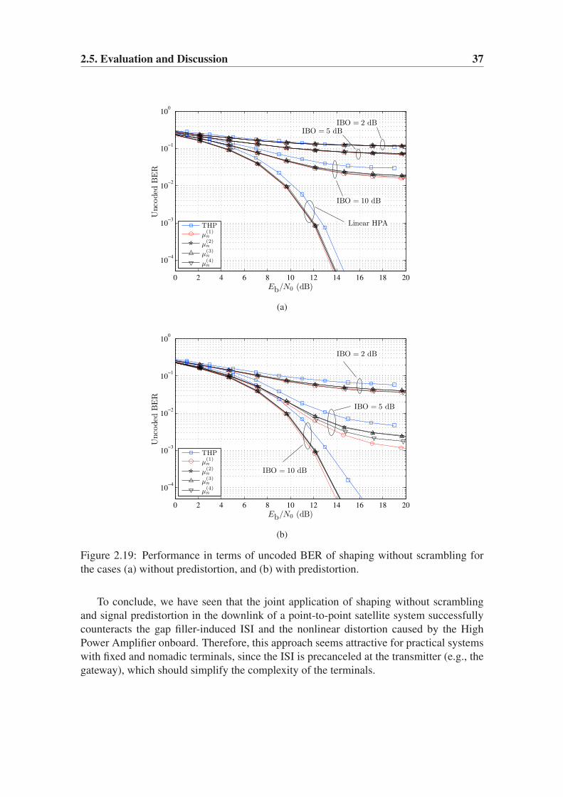
2.5. Evaluation and Discussion 37
0 2 4 6 8 10 12 14 16 18 20
10−4
10−3
10−2
10−1
100
Eb/N0 (dB)
Unco
ded
BE
R
Linear HPA
IBO = 10 dB
IBO = 5 dBIBO = 2 dB
THP
µ(1)n
µ(2)n
µ(3)n
µ(4)n
(a)
0 2 4 6 8 10 12 14 16 18 20
10−4
10−3
10−2
10−1
100
Eb/N0 (dB)
Unco
ded
BE
R
IBO = 10 dB
IBO = 5 dB
IBO = 2 dB
THP
µ(1)n
µ(2)n
µ(3)n
µ(4)n
(b)
Figure 2.19: Performance in terms of uncoded BER of shaping without scrambling for
the cases (a) without predistortion, and (b) with predistortion.
To conclude, we have seen that the joint application of shaping without scrambling
and signal predistortion in the downlink of a point-to-point satellite system successfully
counteracts the gap filler-induced ISI and the nonlinear distortion caused by the High
Power Amplifier onboard. Therefore, this approach seems attractive for practical systems
with fixed and nomadic terminals, since the ISI is precanceled at the transmitter (e.g., the
gateway), which should simplify the complexity of the terminals.

38 Chapter 2. Application of THP to Point-to-Point Satellite Communications
Appendix 2.A Filter Computation for SISO THP
Consider Figure 2.20, which represents the continuous-time signal path between the sym-
bol to waveform conversion at the transmitter and the sampling at the receiver. This
continuous-time path corresponds to the waveform-domain chain of Figures 2.11 and 2.12,
except for the nonlinear blocks (predistortion and HPA), which are not considered here
(i.e., perfect predistortion is assumed). As shown in Figure 2.20, it is possible to describe
the system behavior at baud rate by means of an equivalent discrete-time filter H(z) and
a discrete white noise source.
Figure 2.20: Continuous-time channel (top) and corresponding discrete-time equivalent
channel (bottom) of the considered system.
We assume that the pulse shaping filter HT(f) and the channel HC(f) are fixed and
known, and we want to find the required receive filter HWMF(f) (the whitened matched
filter) and the equivalent discrete-time filter H(z) required by THP and DFE. An over-
sampling factor of 4 was used in the simulations to represent the continuous-time signals.
Pulse shaping filter As pulse shaping filter we consider a SRRC filter with roll-off
α = 0.3. The frequency response of the SRRC filter is the square root of that of the
Raised Cosine (RC) filter of equal roll-off. The RC filter is a real-valued filter with even
symmetry which features Nyquist characteristics (i.e., it introduces no ISI when correctly
sampled at baud rate). The frequency response of a RC filter is given by
HRC(f) =
T, 0 ≤ |f | ≤ 1−α2T
T2
[1 + cos
(πTα
(|f | − 1−α
2T
))], 1−α
2T≤ |f | ≤ 1+α
2T
0, |f | > 1+α2T
. (2.32)
The frequency domain and time domain responses of the SRRC and RC filters are dis-
played in Figure 2.21.

2.A. Filter Computation for SISO THP 39
Channel impulse response The channel response is chosen to comply with the power
delay profile of Figure 2.9. A static tapped delay line is used as time-domain channel
response (with 4 samples per symbol period), i.e.:
hC(t) =10∑
k=1
ρk ejφkδ(t− τk) (2.33)
where ρk ejφk is the k-th complex tap of amplitude ρk and phase φk, and τk is its corre-
sponding delay. Table 2.5 details the parameters of the time-domain impulse response of
the channel (up to an amplitude scaling). As explained in Section 2.3, the tap phases φk
were arbitrarily chosen.
Whitened matched filter The WMF is chosen as receiver front-end. The WMF is
designed to be matched to the transmit chain and, when followed by proper baud rate
sampling, provides samples affected by uncorrelated noise. As shown in Figure 2.22, The
WMF can be thought as a single analog filter HWMF(f) followed by baud rate sampling,
or it can be seen as the concatenation of (i) a continuous-time matched filter HMF(f).=
H∗C(f) · H∗
T(f), (ii) baud rate sampling, and (iii) a discrete-time noise-whitening filter
HNW(z). This latter filter removes the correlation that the matched filter introduces in the
noise component.
Discrete-time channel and noise-whitening filters The noise-whitening filter HNW(z)and the discrete-time equivalent filter H(z) are necessarily related, see Figures 2.20 and 2.22.
In fact, they are found as solutions of a spectral factorization problem applied to a certain
−2 −1.5 −1 −0.5 0 0.5 1 1.5 20
0.2
0.4
0.6
0.8
1
f · T
T·∣ ∣
H(·
)(f
)∣ ∣
Hsrrc(f)Hrc(f)
−10 −9 −8 −7 −6 −5 −4 −3 −2 −1 0 1 2 3 4 5 6 7 8 9 10
0
0.5
1
t/T
h(·
)(t)
hsrrc(t)hrc(t)
Figure 2.21: Frequency-domain (top) and time-domain (bottom) response of the SRRC
and RC filters with roll-off α = 0.3.

40 Chapter 2. Application of THP to Point-to-Point Satellite Communications
Table 2.5: Time-domain impulse response of the channel used for simulation. The as-
sumed symbol rate is 1/T = 3.84 Mbaud.
Tap Nr. τk (µs) τk/T Power (dBm) ρk φk (rad)
1 0 0 −90.909 1 0
2 1.3672 21/4 −62.319 26.8844 0.2315
3 1.6276 25/4 −65.719 18.1761 −2.7677
4 1.6927 26/4 −66.929 15.8125 −2.5826
5 1.8229 28/4 −67.039 15.6135 −1.4369
6 2.1484 33/4 −80.579 3.2487 −0.5713
7 2.2135 34/4 −80.399 3.3535 −0.1631
8 3.5156 54/4 −81.119 3.0867 −1.5745
9 5.0781 78/4 −66.469 16.6725 −0.2711
10 6.7708 104/4 −81.509 2.9512 −0.8634
Figure 2.22: Two equivalent representations of the WMF: single continuous-time front-
end (top), and concatenation of continuous-time matched filter and discrete-time noise-
whitening (bottom).

2.A. Filter Computation for SISO THP 41
discrete-time transfer function U(z), whose definition changes according to the equaliza-
tion criterion.8 We consider in this chapter the ZF and MMSE criteria. The corresponding
transfer functions to be factored are given by (subscripts indicate the criterion)
UZF(z).= σ2
a ·G(z) (2.34)
UMMSE(z).= σ2
a ·G(z) +N0
T(2.35)
where σ2a = E {|an|2}, N0 is the value of the Power Spectral Density (PSD) of the
continuous-time white noise process w0(t), and T is the symbol period.9 G(z) is the
discrete-time transfer function of the system as if the baud rate samples were taken at the
output of the matched filter, see Figure 2.22. It is readily seen that G(z) is proportional to
the PSD of the discrete-time noise component of the baud rate samples at the matched fil-
ter output. If we define G(f) as the continuous-time transfer function of the concatenation
of transmit filter, channel, and matched filter, i.e.,
G(f).= HT(f) ·HC(f) ·HMF(f) = |HT(f) ·HC(f)|2 (2.36)
then G(z) can be seen as the baud rate equivalent transfer function of G(f). If G(z) is
evaluated in the unit circle, we obtain the discrete-time frequency response of the sampled
system G(ej2πT ), which is related to G(f) by
G(ej2πfT ) =∑
µ
G(f − µ
T
)=∑
µ
∣∣HT
(f − µ
T
)·HC
(f − µ
T
)∣∣2. (2.37)
Figure 2.23 shows the magnitudes of the overall continuous-time transfer function G(f)(top) and its periodic continuation in continuous-time obtained after baud rate sampling
(middle). The time-dispersive nature of the channel response HC(f) is evident. The
inverse of the periodic continuation of G(f) is displayed at the bottom of Figure 2.23 to
show the importance of the deep notch that G(f) presents about f · T = 0.06, which
would cause severe noise enhancement if ZF linear equalization were used.
Regardless of the equalization criterion, U(z) must be factored as follows:
σ2a · U(z) = σ2
h ·H(z) ·H∗(1/z∗) (2.38)
where σ2h is a positive constant (with the dimensions of variance), and H(z) is the desired
equivalent discrete-time impulse response required for THP and DFE. If we recall Sec-
tion 2.2.1.2, H(z) is required to be causal and minimum-phase with h0 = 1. This implies
that U(z) must be factored into two transfer functions: H(z) containing all the zeros of
U(z) lying inside the unit circle, and H∗(1/z∗), which contains the zeros of U(z) outside
the unit circle. The factor σ2h is introduced to ensure that H(z) is a monic polynomial
(i.e., h0 = 1). Figure 2.24 displays G(ej2πfT ) as well as the location of the roots of G(z),which coincide with the roots of UZF(z) since both transfer functions are proportional.
8We note that the filters H(z) and HNW(z) provided by the factorization procedure are valid for both the
THP and DFE implementations of Figures 2.11 and 2.12.9Note once again that UMMSE(z) converges asymptotically to UZF(z) as the SNR approaches infinity (i.e.,
as N0 → 0).
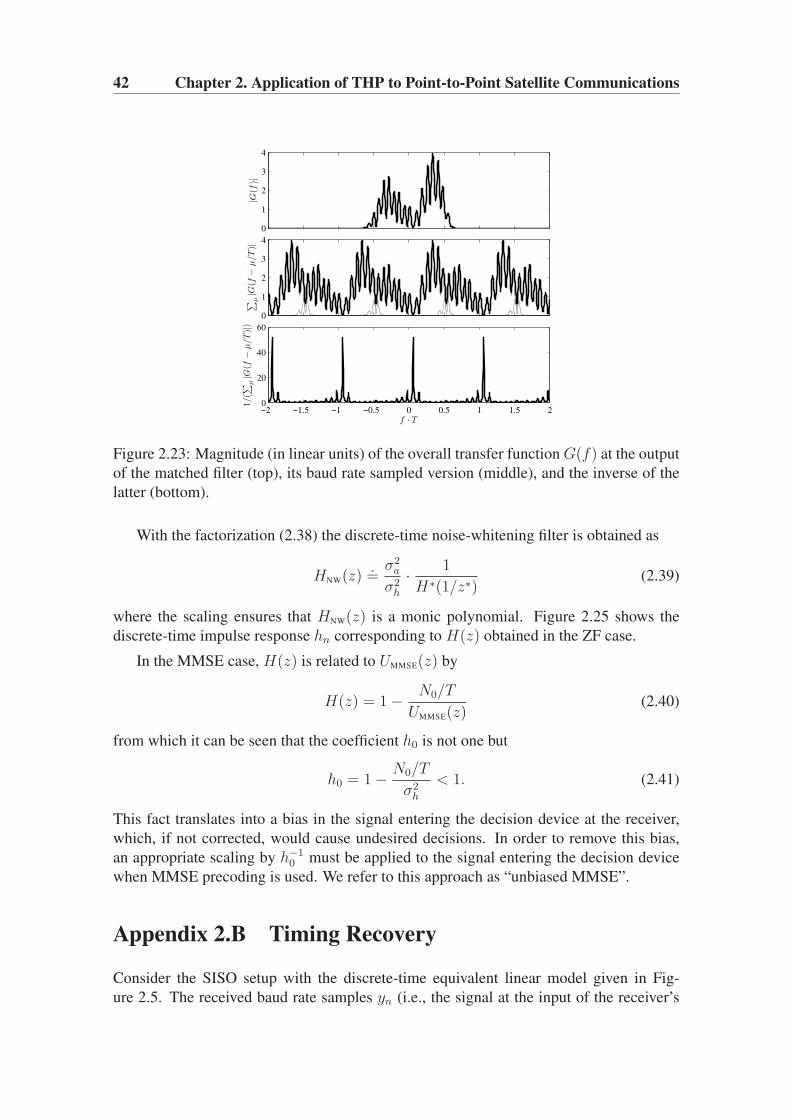
42 Chapter 2. Application of THP to Point-to-Point Satellite Communications
0
1
2
3
4
|G(f
)|
0
1
2
3
4∑
µ|G
(f−
µ/T
)|
−2 −1.5 −1 −0.5 0 0.5 1 1.5 20
20
40
60
1/(
∑
µ|G
(f−
µ/T
)|)
f · T
Figure 2.23: Magnitude (in linear units) of the overall transfer function G(f) at the output
of the matched filter (top), its baud rate sampled version (middle), and the inverse of the
latter (bottom).
With the factorization (2.38) the discrete-time noise-whitening filter is obtained as
HNW(z).=
σ2a
σ2h
· 1
H∗(1/z∗)(2.39)
where the scaling ensures that HNW(z) is a monic polynomial. Figure 2.25 shows the
discrete-time impulse response hn corresponding to H(z) obtained in the ZF case.
In the MMSE case, H(z) is related to UMMSE(z) by
H(z) = 1− N0/T
UMMSE(z)(2.40)
from which it can be seen that the coefficient h0 is not one but
h0 = 1− N0/T
σ2h
< 1. (2.41)
This fact translates into a bias in the signal entering the decision device at the receiver,
which, if not corrected, would cause undesired decisions. In order to remove this bias,
an appropriate scaling by h−10 must be applied to the signal entering the decision device
when MMSE precoding is used. We refer to this approach as “unbiased MMSE”.
Appendix 2.B Timing Recovery
Consider the SISO setup with the discrete-time equivalent linear model given in Fig-
ure 2.5. The received baud rate samples yn (i.e., the signal at the input of the receiver’s
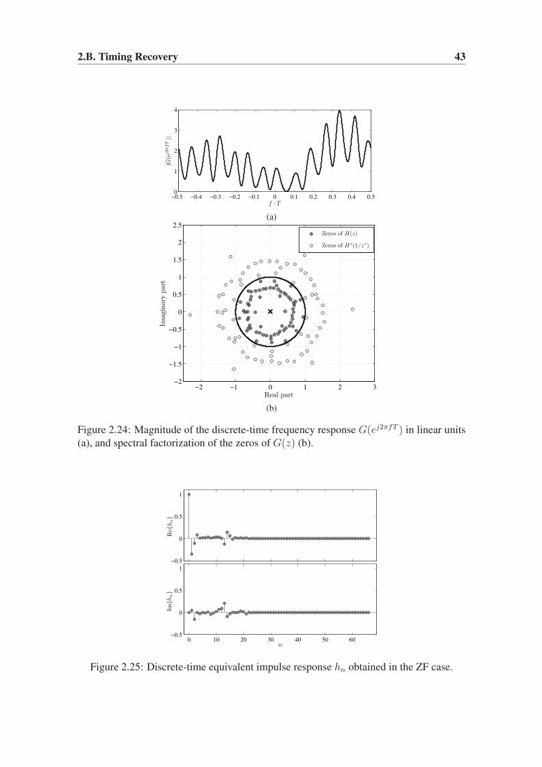
2.B. Timing Recovery 43
−0.5 −0.4 −0.3 −0.2 −0.1 0 0.1 0.2 0.3 0.4 0.50
1
2
3
4
|G(e
j2πfT
)|
f · T
(a)
−2 −1 0 1 2 3−2
−1.5
−1
−0.5
0
0.5
1
1.5
2
2.5
Real part
Imag
inar
ypar
t
Zeros of H(z)
Zeros of H∗(1/z∗)
(b)
Figure 2.24: Magnitude of the discrete-time frequency response G(ej2πfT ) in linear units
(a), and spectral factorization of the zeros of G(z) (b).
−0.5
0
0.5
1
Re{
hn}
0 10 20 30 40 50 60−0.5
0
0.5
1
n
Im{h
n}
Figure 2.25: Discrete-time equivalent impulse response hn obtained in the ZF case.

44 Chapter 2. Application of THP to Point-to-Point Satellite Communications
modulo device) turns out to be a noisy version of the effective data sequence vn. As men-
tioned in Section 2.2.1.2, the effective symbols vn follow a discrete Gaussian distribution
taking values on the set of points which are modulo congruent to the original QAM con-
stellation. Figure 2.26 shows a typical scatter plot for yn assuming perfect timing recov-
ery. Three different ISI conditions are shown, corresponding with three different channel
transfer functions: (a) no ISI (i.e., H(z) = 1), (b) weak ISI conditions, and (c) strong ISI
conditions. The transfer function providing strong ISI conditions is that considered for
evaluation in the main text of this chapter, which is extracted from the time-domain over-
sampled impulse response provided in Table 2.5. The transfer function providing weak
ISI conditions is extracted from the oversampled impulse response given in Table 2.6.10 In
Figure 2.26 it is observed that the received discrete Gaussian becomes more spread as the
amount of ISI increases, as it was noted in Section 2.2.1.2. The application of THP turns
out to pose important hurdles to the timing acquisition task. In this section we provide an
overview of the timing acquisition problem in SISO THP systems.
−3 −2 −1 0 1 2 3−3
−2
−1
0
1
2
3
In-Phase
Quadra
ture
(a) No ISI
−3 −2 −1 0 1 2 3−3
−2
−1
0
1
2
3
In-Phase
Quadra
ture
(b) Weak ISI
−3 −2 −1 0 1 2 3−3
−2
−1
0
1
2
3
In-Phase
Quadra
ture
(c) Strong ISI
Figure 2.26: Typical scatter plot of the symbols yn at the input of the modulo device
of the receiver, for 16-QAM THP transmission with perfect timing synchronization and
Eb/N0 = 20 dB. Three cases are shown: (a) ISI-free conditions; (b) weak ISI conditions;
(c) strong ISI conditions. The dashed square represents the limits of the modulo operation.
Symbol timing recovery can be performed in continuous (or feedback) or in block-
wise (or feedforward) fashion. In continuous mode the estimate is repeatedly updated af-
ter each newly received sample, whereas burst-mode estimators are suitable for operation
over finite blocks of observed samples. Most practical recovery schemes use a feedback
loop composed of a timing error detector followed by a loop filter to control the sampling
instants of the incoming signal [74, 126]. Such configuration derives from Phase-Locked
Loop (PLL)-based techniques traditionally used in analog transmission, and exhibits sim-
ilar operational issues. One of such issues is the inherent trade-off between two antago-
nistic goals: on one hand, the ability to cope with quick timing offset variations requires a
sufficiently large loop filter bandwidth; on the other hand, the jitter of the offset estimates
10As in the case of the reference channel response of Table 2.5, this channel impulse response has been
kindly provided by the Digicomm research group of the DEIS Department at the University of Bologna. In
this case, the channel response has been obtained using rural terrain data, which is typically associated to
less multipath, and hence, less ISI.

2.B. Timing Recovery 45
Table 2.6: Time-domain impulse response of the channel corresponding to weak ISI con-
ditions. The assumed symbol rate is 1/T = 3.84 Mbaud.
Tap Nr. τk (µs) τk/T Power (dBm) ρk φk (rad)
1 0 0 −91.949 1 0
2 0.1953 3/4 −106.329 0.1910 0.2315
3 0.2604 4/4 −110.129 0.1233 −2.7677
4 0.8464 13/4 −112.519 0.0936 −2.5826
5 1.1719 18/4 −110.179 0.1226 −1.4369
6 1.9531 30/4 −112.519 0.0936 −0.5713
7 2.8646 44/4 −112.519 0.0936 −0.1631
grows with the loop bandwidth. In practice, a two step approach is often adopted: first, a
coarse timing recovery phase is performed using a large loop bandwidth in order to rapidly
obtain a first timing estimate, after which a smaller loop bandwidth is used to provide a
steady-state timing with low jitter. Feedforward schemes exhibit a similar trade-off be-
tween loop bandwidth and estimate error variance, but, in contrast to feedback schemes,
they avoid the slow start-up phase. This fact makes them attractive for application under
certain conditions, especially for burst-mode operation [106, 121, 128, 145, 165]. As for
the sampling rate of the input signal, symbol timing recovery can be performed using the
oversampled output of the matched filter [74,106,128,145,165], or the baud rate samples
at the output of the matched filter [93, 126]. According to the knowledge of the trans-
mitted data, we can distinguish among Data-aided (DA) timing recovery (known pilot
symbols), Decision-directed (DD) timing recovery (symbol decisions at the receiver play
the role of known symbols) [126], and Non-data-aided (NDA) mode (no knowledge is
assumed) [106, 124, 125, 128, 145, 165].
The problem of timing acquisition in THP systems has been hardly covered in the
open literature. In coincidence with the recent standardization of the 10GBASE-T tech-
nology [90], the first works on the topic are being published. To the best of the author’s
knowledge, the two contributions by Chien et et al. [36,38] constitute the only references
on the topic. Whereas in [36] the authors focus on the problem of joint timing recovery of
four interdependent data streams11, in [38] the authors present a DD baud rate timing re-
covery scheme particularly designed for SISO THP transmission. The algorithm is based
on the classical Mueller and Muller (M&M) timing detector applied to the effective THP
data sequence, and it apparently outperforms by far other timing recovery schemes not
specifically derived for THP.
O&M timing recovery for THP signals In order to illustrate the difficulties that clas-
sical timing acquisition schemes face when applied to THP signals we consider here the
Oerder and Meyr (O&M) scheme [128] applied to a SISO ZF-THP system. Figure 2.27
11The 10GBASE-T standard [90] considers, among other cablings, the use of four-pair copper lines,
which may interfere with each other.

46 Chapter 2. Application of THP to Point-to-Point Satellite Communications
Figure 2.27: Linear signal model considered for timing acquisition.
shows the considered signal model. The O&M scheme operates on the oversampled out-
put of the matched filter q(t = kTs), where Ts is the oversampling rate. G(f) is the
cascade of transmit, channel and matched filters, i.e., G(f) = HT(f)HC(f)HMF(f) [re-
call (2.36)]. Hence, the output of the matched filter can be written as
q(t) =∑
n
xng(t− nT ) + w(t) (2.42)
where g(t) is the time domain impulse response corresponding to G(f), and w(t) rep-
resents the colored Gaussian noise component at the output of the matched filter. Now,
considering the relationship between vn and xn given by (2.8), i.e., vn =∑p−1
k=0 hkxn−k,
let us define h(−1)n as the discrete-time impulse response of the inverse of the channel,
which allows to write xn =∑
k h(−1)k vn−k. Alternatively, h
(−1)n can be considered as the
inverse Z-transform of 1/H(z). Now, using h(−1)n it is possible to rewrite the ISI-free
signal (2.42) in terms of vn as follows
q(t) =∑
n
(∑
m
vmh(−1)n−m
)
g(t− nT ) + w(t)
=∑
m
vm
(∑
n
h(−1)n−mg(t− nT )
)
+ w(t)
=∑
m
vm
(∑
k
h(−1)k g(t− kT −mT )
)
+ w(t) (2.43)
=∑
m
vmp(t−mT ) + w(t) (2.44)
where in (2.43) we have used the change of index k = n−m. The continuous-time pulse
p(t).=∑
k h(−1)k g(t− kT ) represents the equivalent impulse response of the cascade of
the (linear) precoding operation, transmit filter, channel response, and matched filter, as
indicated in Figure 2.27 by its frequency response P (f).
The O&M scheme extracts the timing estimate ǫ in a feedforward, blockwise manner
as follows
ǫm = − 1
2πarg
(m+1)NsL−1∑
k=mNsL
|q(kTs)|2 exp
(
−j2πk
Ns
)
(2.45)

2.B. Timing Recovery 47
0 5 10 15 20 25 30
10−2
10−1
Eb/N0 (dB)
Sta
ndard
dev
iati
on
ofth
ees
tim
ate
s
THP, strong ISITHP, weak ISIPlain 16-QAM, strong ISIPlain 16-QAM, weak ISIPlain 16-QAM, no ISI
Figure 2.28: Standard deviation of the O&M estimates (L = 100, Ns = 4) under 16-QAM
THP transmission through channels introducing different amounts of ISI.
with m the block index, L the block length in symbol intervals, Ns the oversampling
factor, and Ts = T/Ns the oversampling interval (Ns ≥ 2). The estimate ǫm is used as
the sampling offset for all the symbols within the observation block. The variance of the
O&M estimate is in general inversely proportional to the estimation block length L, and
can be seen to be contributed by three components [128]
Var {ǫ} .= σ2
O&M = σ2n×n + σ2
s×n + σ2s×s
of which the first term σ2n×n is due to noise self-interaction, and dominates in the small
SNR region; the term σ2s×n is due to the interaction between the signal and noise compo-
nents, and dominates at intermediate SNRs; and the term σ2s×s is due to self-interaction of
the signal component, and dominates in the high SNR region. The last term is independent
of the SNR, and thus represents a performance floor at high SNRs.
In general, the variance of the O&M estimate, and especially its (s × s) contribu-
tion, depends on the covariance of the symbols and the overall impulse response of the
transmission chain [128]. In the case of THP transmission, the effective data sequence
vn is correlated through the equivalent transfer function H(z), see (2.8). But since this
transfer function depends on the overall impulse response G(f), see Appendix 2.A, the
contributions of the symbol covariance and the channel response are not fully separable.
Figure 2.28 displays the influence of the amount of ISI introduced by the channel
in the performance achieved by O&M timing recovery in terms of standard deviation of
the estimates. Three cases are shown corresponding to the three levels of ISI (strong,
weak, nonexistent) of Figure 2.26 both for THP and plain 16-QAM transmission (in the
ISI-free case, THP reduces to plain 16-QAM). The cases of plain 16-QAM transmission
with ISI correspond to the case where sampling would be performed prior to (baud-rate)
equalization. The curves were obtained through simulation with L = 100 symbols and
Ns = 4. The bias is negligible for SNRs above 0 dB for THP transmission, but not for
plain 16-QAM transmission under ISI conditions. Figure 2.28 shows that the standard
deviation at high SNRs for the cases with ISI lies above that of the ISI-free case. Such

48 Chapter 2. Application of THP to Point-to-Point Satellite Communications
performance gap reveals a direct influence of the amount of ISI in the (s× s) contribution
to the timing jitter. Surprisingly, a comparison between the THP and plain 16-QAM
cases under equal ISI conditions shows that the performance of O&M under weak ISI is
worse for THP than for plain 16-QAM, whereas under strong ISI it is better for THP than
for plain 16-QAM. A variance analysis similar to that performed in [128] for the plain
QAM case would be needed to fully explain and quantify the observed gaps, although the
mathematical developments would be rather cumbersome. Although it may seem from
Figure 2.28 that the performance floor increases with the amount of ISI, this rule does not
hold in general.
0
1
2
3
Sam
ple
rin
put
−0.02
0
0.02
0.04
Est
imate
doffse
t
50 100 150 200 250 300 350
0.05
0.1
0.15
Sym
boler
ror
Symbol number
Figure 2.29: Time series of a 16-QAM THP received signal under strong ISI conditions
and O&M timing recovery (L = 50 symbols, Ns = 4). Shown are (a) the magnitude of the
oversampled received signal q(kTs) (gray), and the magnitude of the baud rate samples
(black dots), (b) the estimated offsets for each symbol block, and (c) the magnitude of the
error between the true and the sampled symbols. No noise was present in the simulation,
and the true offset was set to ǫ = 0.
One of the reasons that may explain the worse performance of O&M under THP trans-
mission is that the signal at the matched filter output (which amounts to a noisy version
of vk modulated by a raised cosine filter) does not seem to be cyclostationary.12 Such
non-cyclostationarity would be in agreement with the analysis performed in [158], where
it is concluded that the precoded sequence xk is only cyclostationary for some partic-
ular channels H(z) with integer coefficients. In our case, the coefficients of H(z) are
not (complex) integers in general, so that the xk, and thus vk, can be considered non-
12A signal is said to be cyclostationary when its statistical characteristics vary periodically with time [75].

2.B. Timing Recovery 49
0 5 10 15 20 25 30
10−2
Eb/N0 (dB)
Sta
ndard
dev
iati
on
ofth
ees
tim
ate
s
QPSK16-QAM64-QAM256-QAMTHPPlain QAM
Figure 2.30: Standard deviation of the O&M estimates under THP transmission with
different QAM constellations.
cyclostationary. This fact is important in terms of timing recovery since it could explain
the sudden increase in the error of the timing estimates for some O&M estimation blocks.
One such event can be observed in Figure 2.29, which represents a snapshot of the perfor-
mance of the O&M estimator during several estimation blocks (of length L = 50). The
largest offset error is obtained for the last block of symbols (about 0.04T ), which happens
to exhibit a large number of effective symbols with large magnitude. In contrast, blocks
with fewer such symbols provide more accurate offset estimates. In our simulations we
have observed that the occasional appearance of a symbol with large amplitude can have
a negative impact in the accuracy of the O&M timing estimate for its estimation block.
However, we acknowledge that a complete statistical analysis would be needed in order to
completely explain the behavior of O&M timing recovery under THP transmission. This
task is left here as a topic for future research.
Figure 2.30 shows the performance in terms of standard deviation of the O&M es-
timates for different TH-precoded QAM modulations under strong ISI conditions. For
comparison, the performance for plain ISI-free QAM transmission is also shown. The
curves were obtained through simulation with L = 100 and Ns = 4. The bias turns out to
be negligible for SNRs above 0 dB in all tested cases. The high SNR gap of the O&M esti-
mates for THP with respect to plain QAM can be observed for all constellations, although
the gap decreases as the QAM constellation size increases.
Figure 2.31 displays the dependence of the O&M estimator with respect to the length
of the estimation block, L. It can be observed that the performance loss of THP with
respect to plain QAM is negligible at low SNRs, but not at high SNRs, where the standard
deviation gap varies between a factor of 1.5 and 2.
The recent M&M-based timing recovery scheme presented in [38] successfully ex-
ploits the correlation in the effective data sequence, achieving a considerable improve-
ment over other state-of-the art schemes, and thus appears to be the best current recovery
scheme suitable for implementation in THP systems.
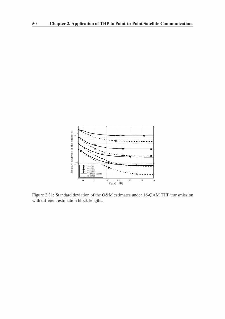
50 Chapter 2. Application of THP to Point-to-Point Satellite Communications
0 5 10 15 20 25 30
10−2
10−1
Eb/N0 (dB)
Sta
ndard
dev
iati
on
ofth
ees
tim
ate
s
L = 20L = 50L = 100L = 200THP (16-QAM)16-QAM
Figure 2.31: Standard deviation of the O&M estimates under 16-QAM THP transmission
with different estimation block lengths.

Chapter 3Application of Tomlinson-Harashima
Precoding to Multibeam Satellite
Communications
Contents
3.1 Introduction . . . . . . . . . . . . . . . . . . . . . . . . . . . . . . . 52
3.2 Theoretical Background: THP for Multibeam Systems . . . . . . . 54
3.2.1 Signal Model . . . . . . . . . . . . . . . . . . . . . . . . . . . 54
3.2.2 Linear Transmitter Precoding . . . . . . . . . . . . . . . . . . 56
3.2.3 Nonlinear Transmitter Precoding: THP . . . . . . . . . . . . . 57
3.3 Multibeam Downlink Scenario Description . . . . . . . . . . . . . . 60
3.3.1 Multibeam coverage . . . . . . . . . . . . . . . . . . . . . . . 61
3.3.2 Satellite system details . . . . . . . . . . . . . . . . . . . . . . 62
3.3.3 Particular evaluation scenarios . . . . . . . . . . . . . . . . . . 64
3.4 Considered THP Implementations . . . . . . . . . . . . . . . . . . . 65
3.5 Results and Discussion . . . . . . . . . . . . . . . . . . . . . . . . . 69
Appendix 3.A Filter Computation for MIMO THP . . . . . . . . . . . . 74
3.A.1 “Best-first” Ordering . . . . . . . . . . . . . . . . . . . . . . . 74
3.A.2 Feedforward Matrix Computation for “MMSE-THP-Jo” . . . . 75
Appendix 3.B Receiver Locations for Scenarios S1, S2 and S3 . . . . . . 75
Appendix 3.C Beamforming Implementation . . . . . . . . . . . . . . . 77
Appendix 3.D Nonlinear Distortion in the Multibeam Downlink Scenario 80
3.D.1 Possible Approaches to Predistortion . . . . . . . . . . . . . . 81
Appendix 3.E CSI Knowledge . . . . . . . . . . . . . . . . . . . . . . . . 83

52 Chapter 3. Application of THP to Multibeam Satellite Communications
3.1 Introduction
Whereas in the previous chapter we have considered point-to-point transmissions affected
by time dispersion, in this chapter we will focus on the case of multibeam satellite trans-
mission affected by Co-Channel Interference (CCI). The combination of multibeam cov-
erage with frequency reuse has proven a successful approach to increase the throughput
of current GEO satellite communication systems. As examples we can mention the near
200 beams implemented by the Inmarsat 4 satellites [78], or the more than 500 beams
provided by the TerreStar-1 satellite [156].
Figure 3.1 represents the main elements in the forward link of a GEO multibeam satel-
lite system. The total coverage area is divided in smaller cells, which will be referred to
as spotbeams. Each spotbeam is illuminated by a different beam coming from the satellite
antenna, which is composed of typically between 100 and 200 radiating elements [44].
The beam pattern of the service link (satellite to terminals) is achieved by the combined
action of the radiating elements in the satellite antenna and a beamforming stage which
properly combines the signals to be transmitted before being fed to the radiating elements.
Although the power radiated by each beam is maximum on its spotbeam, part of it spreads
over other beams due to the sidelobes of the radiation pattern.
The data content towards the beams is provided by several gateways through the so-
called feeder links (gateway to satellite). The number of gateways is in general smaller
than the number of beams. The transmitted signals may vary from beam to beam due
to, e.g., service differentiation among countries. Hence, a gateway must feed the satellite
with several independent signals, which requires the implementation of some kind of
multiplexing (typically in frequency and polarization). As a consequence of the service
differentiation among beams, the signals from adjacent beams may become an unwanted
source of disturbance (CCI).
Multibeam coverage benefits from the smaller size of the spotbeam, which allows
to achieve higher radiation gains. In contrast, this may induce a higher CCI in adja-
cent beams. For this reason, most practical systems employ a regular frequency reuse
pattern with Nfr frequencies, which prevents two adjacent beams from reusing the same
frequency.1 In this case, the frequency reuse factor Nfr (also known as cluster size) is of
the form Nfr = m2+mn+n2, with m,n = 0, 1, 2, . . . As a rule of thumb, the dependence
of the throughput, C, of a multibeam system with the beam radius, R, and Nfr is of the
form [113]
C ∝ N−1fr ·R−2.
In terms of throughput, it is therefore desirable that Nfr and R be as small as possible.
However, reducing Nfr or R will cause an undesirable increase in the CCI level, so, in
practice, a trade-off must be met between these two conflicting goals.
In this chapter we propose the application of Tomlinson-Harashima Precoding (THP)
to precompensate the CCI existing in the forward link of a multibeam satellite transmis-
sion system, in which the satellite antenna is to provide different data streams to non-
collaborative receivers located in different spotbeams. The same principles presented in
1In Figure 3.1 colors are used to represent the different frequencies used in each beam.

3.1. Introduction 53
Feeder links
Service links
SpotbeamsReceivers
Multibeam antenna
Beam
Gateway
Gateway
Figure 3.1: Simplified representation of the forward link of a multibeam satellite trans-
mission system.
Chapter 2 apply in the multibeam scenario, with the CCI playing the role of the ISI, as we
will see. The fact that the CCI is precompensated by the THP transmitter offers poten-
tial throughput increases, since the frequency reuse factor (or, equivalently, the spotbeam
radius) could be reduced without sacrificing system performance. To the best of the au-
thor’s knowledge, the application of THP to the forward link of a multibeam satellite
system is a novelty in the related literature. A similar approach, but restricted to linear
precoding techniques, was explored in [43, 67] with promising results. Furthermore, the
problem of CCI cancellation in the reverse link of a multibeam system has been dealt with
in [120, 123] using multiuser detection and decoding techniques.
Chapter outline The chapter is structured as follows. In Section 3.2 we provide the
basic principles of THP applied to multibeam systems. The particular realistic multibeam
system used for reference is described in Section 3.3, and several application scenarios are
selected for evaluation. In Section 3.4 we propose several possible THP implementation
schemes suitable to be applied to the described scenario. Such systems are evaluated
in Section 3.5 by means of numerical simulations. This chapter is based on the work
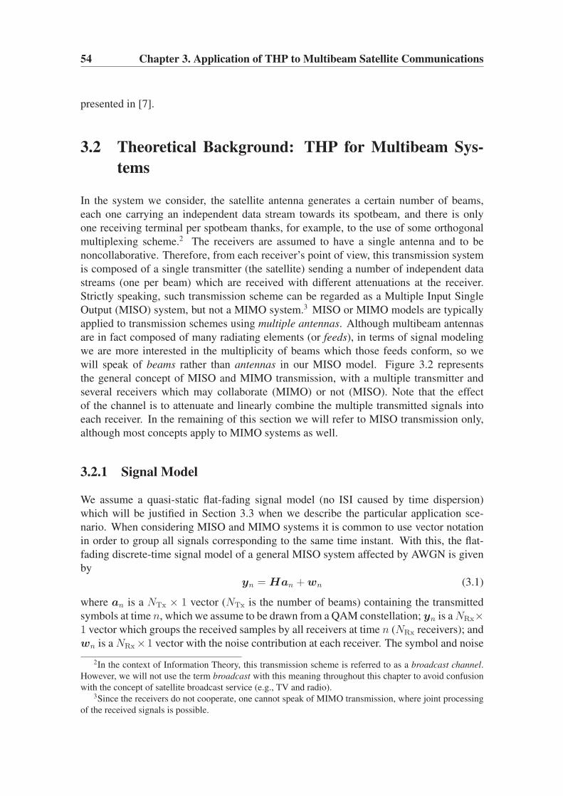
54 Chapter 3. Application of THP to Multibeam Satellite Communications
presented in [7].
3.2 Theoretical Background: THP for Multibeam Sys-
tems
In the system we consider, the satellite antenna generates a certain number of beams,
each one carrying an independent data stream towards its spotbeam, and there is only
one receiving terminal per spotbeam thanks, for example, to the use of some orthogonal
multiplexing scheme.2 The receivers are assumed to have a single antenna and to be
noncollaborative. Therefore, from each receiver’s point of view, this transmission system
is composed of a single transmitter (the satellite) sending a number of independent data
streams (one per beam) which are received with different attenuations at the receiver.
Strictly speaking, such transmission scheme can be regarded as a Multiple Input Single
Output (MISO) system, but not a MIMO system.3 MISO or MIMO models are typically
applied to transmission schemes using multiple antennas. Although multibeam antennas
are in fact composed of many radiating elements (or feeds), in terms of signal modeling
we are more interested in the multiplicity of beams which those feeds conform, so we
will speak of beams rather than antennas in our MISO model. Figure 3.2 represents
the general concept of MISO and MIMO transmission, with a multiple transmitter and
several receivers which may collaborate (MIMO) or not (MISO). Note that the effect
of the channel is to attenuate and linearly combine the multiple transmitted signals into
each receiver. In the remaining of this section we will refer to MISO transmission only,
although most concepts apply to MIMO systems as well.
3.2.1 Signal Model
We assume a quasi-static flat-fading signal model (no ISI caused by time dispersion)
which will be justified in Section 3.3 when we describe the particular application sce-
nario. When considering MISO and MIMO systems it is common to use vector notation
in order to group all signals corresponding to the same time instant. With this, the flat-
fading discrete-time signal model of a general MISO system affected by AWGN is given
by
yn = Han +wn (3.1)
where an is a NTx × 1 vector (NTx is the number of beams) containing the transmitted
symbols at time n, which we assume to be drawn from a QAM constellation; yn is a NRx×1 vector which groups the received samples by all receivers at time n (NRx receivers); and
wn is a NRx×1 vector with the noise contribution at each receiver. The symbol and noise
2In the context of Information Theory, this transmission scheme is referred to as a broadcast channel.
However, we will not use the term broadcast with this meaning throughout this chapter to avoid confusion
with the concept of satellite broadcast service (e.g., TV and radio).3Since the receivers do not cooperate, one cannot speak of MIMO transmission, where joint processing
of the received signals is possible.

3.2. Theoretical Background: THP for Multibeam Systems 55
Figure 3.2: Representation of MIMO and MISO transmission. MIMO: collaborative re-
ceivers, or single receiver with multiple antennas. MISO: non collaborative single antenna
receivers.
sequences have zero mean and are white in the time domain and also in the space domain
(i.e., E{aaH
}= σ2
aI and E{wwH
}= σ2
wI). The QAM constellation is assumed to be
normalized in energy (σ2a = 1).
The flat-fading channel, which comprises the effects of the beam radiation patterns
and the propagation, is represented by the NRx × NTx matrix H whose elements hij
contain the complex attenuations from the j-th beam to the i-th receiving terminal, with
i = 1, 2, . . . , NRx, and j = 1, 2, . . . , NTx.4 For example, consider the i-th element of yn,
which is given by
[yn]i =
NTx∑
j=1
hij [an]j + [wn]i . (3.2)
It is clear that the effect of the channel is to mix the signals coming from all beams into
each receiving terminal.
In our case, the previous general model can be slightly simplified since we consider
that there is one receiver per beam. Letting NB be the number of beams, we have that
NTx = NRx = NB, and hence x and y are NB × 1 vectors, and H is an NB ×NB square
matrix.
In MISO systems the precoding operation can be considered as a spatial-domain ver-
sion of time-domain preequalization already introduced in Section 2.2.1.1. By “space”
we are referring to the beams. Whereas in time-domain preequalization a time-domain
4If the flat-fading assumption were not valid, then one should consider a matrix transfer function of the
form H(z) =∑
k Hk · z−k, whose entries are scalar transfer functions, i.e., [H]ij (z) =∑
k[Hk]ijz−k.
Precoding schemes designed to counteract both time and spatial dispersion exist in the literature, e.g. [96],
although we restrict our analysis to the flat-fading model.
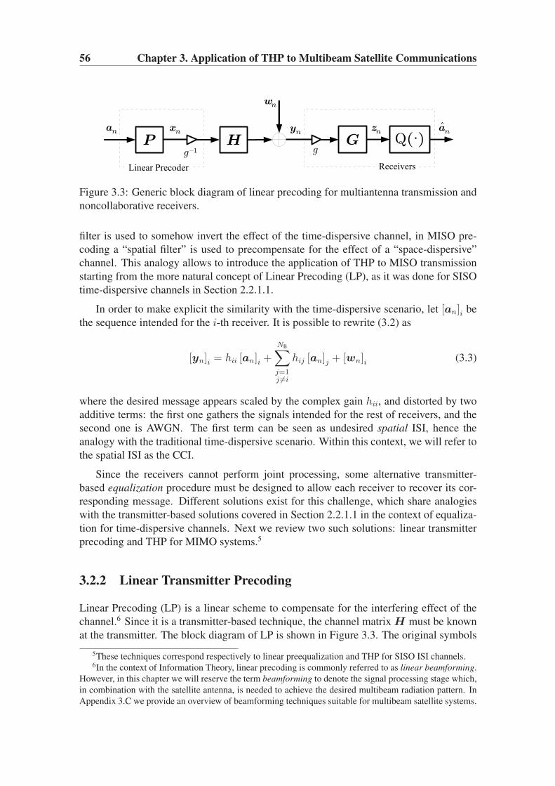
56 Chapter 3. Application of THP to Multibeam Satellite Communications
Figure 3.3: Generic block diagram of linear precoding for multiantenna transmission and
noncollaborative receivers.
filter is used to somehow invert the effect of the time-dispersive channel, in MISO pre-
coding a “spatial filter” is used to precompensate for the effect of a “space-dispersive”
channel. This analogy allows to introduce the application of THP to MISO transmission
starting from the more natural concept of Linear Precoding (LP), as it was done for SISO
time-dispersive channels in Section 2.2.1.1.
In order to make explicit the similarity with the time-dispersive scenario, let [an]i be
the sequence intended for the i-th receiver. It is possible to rewrite (3.2) as
[yn]i = hii [an]i +
NB∑
j=1j 6=i
hij [an]j + [wn]i (3.3)
where the desired message appears scaled by the complex gain hii, and distorted by two
additive terms: the first one gathers the signals intended for the rest of receivers, and the
second one is AWGN. The first term can be seen as undesired spatial ISI, hence the
analogy with the traditional time-dispersive scenario. Within this context, we will refer to
the spatial ISI as the CCI.
Since the receivers cannot perform joint processing, some alternative transmitter-
based equalization procedure must be designed to allow each receiver to recover its cor-
responding message. Different solutions exist for this challenge, which share analogies
with the transmitter-based solutions covered in Section 2.2.1.1 in the context of equaliza-
tion for time-dispersive channels. Next we review two such solutions: linear transmitter
precoding and THP for MIMO systems.5
3.2.2 Linear Transmitter Precoding
Linear Precoding (LP) is a linear scheme to compensate for the interfering effect of the
channel.6 Since it is a transmitter-based technique, the channel matrix H must be known
at the transmitter. The block diagram of LP is shown in Figure 3.3. The original symbols
5These techniques correspond respectively to linear preequalization and THP for SISO ISI channels.6In the context of Information Theory, linear precoding is commonly referred to as linear beamforming.
However, in this chapter we will reserve the term beamforming to denote the signal processing stage which,
in combination with the satellite antenna, is needed to achieve the desired multibeam radiation pattern. In
Appendix 3.C we provide an overview of beamforming techniques suitable for multibeam satellite systems.

3.2. Theoretical Background: THP for Multibeam Systems 57
are fed to a linear spatial filter (matrix P , which in our case is NB × NB) whose role is
to precompensate the effect of the channel (matrix H). The positive scalar factor g−1 at
the transmitter is applied in order to meet the transmit power limitation (represented by
ETX) present in a practical transmitter.7 Its effect is undone at the receiver by applying the
inverse scalar factor g. We consider here two approaches to LP (see [99] for a complete
derivation):
• Zero-forcing LP (ZF-LP). The transmit filter and scaling constant are given by
P ZF-LP = H+ .= HH(HHH)−1 (3.4)
gZF-LP =
√
Tr ((HHH)−1σ2a)
ETX
(3.5)
where H+ is the so-called Moore-Penrose pseudoinverse of H . Note that if H is
invertible, then H+ reduces to H−1, which clearly reveals the ZF nature of this
approach.
• Minimum mean square error LP (MMSE-LP). Under this approach, the noise
variance σ2w (which, in addition to H , must be known by the transmitter) is taken
into account so as to improve the performance of the ZF approach in the low SNR
region. In this case the expressions of the transmit filter and scaling constant are
given by:
PMMSE-LP = (HHH + ξI)−1HH (3.6)
gMMSE-LP =
√
Tr ((HHH + ξI)−2HHHσ2a)
ETX
(3.7)
where ξ.= NBσ
2w/ETX. As expected, the MMSE and ZF solutions coincide asymp-
totically as the SNR grows (i.e., when σ2w → 0).
In general, the main drawback of LP is the increase in average energy of the precoded sig-
nal with respect to the original signal due to the channel inversion. This effect becomes
stronger as the level of CCI increases. Considering the satellite scenario, where transmit
power is a precious resource, this effect should be avoided. Not surprisingly, such draw-
back is shared by the ZF approach to preequalization for SISO ISI channels, as we have
seen in Section 2.2.1.1.
3.2.3 Nonlinear Transmitter Precoding: THP
This latter problem of LP can be avoided if nonlinear precoding is used at the transmitter.
Similarly to the SISO case of Section 2.2.1, the main advantage of nonlinear precoding
(and in particular, THP) is that the energy of the precoded signal is kept almost at the
same level as that of the original signal. Again, perfect knowledge of the channel matrix
H is assumed (full Channel State Information knowledge). We refer to Appendix 3.E for
details on the channel estimation procedure.
7Although its effect could well be integrated within the transmit filter P , we have intentionally repre-
sented both operations separately to make explicit the transmit power requirements.

58 Chapter 3. Application of THP to Multibeam Satellite Communications
Figure 3.4: Generic block diagram of THP applied to a multiantenna transmission and
noncollaborative receivers.
Figure 3.4 depicts the generic block diagram of THP applied to a MIMO system. A
block-by-block description follows:
• Signal reordering. First, the rows of the original QAM vector an are reordered by
means of the NB × NB permutation matrix Π. This operation, which is a novelty
with respect to LP, selects the order in which the different components of an will be
precoded, since the overall performance depends in general on the precoding order.
Since the reordering is transparent to the receivers, it can be seen as a degree of
freedom available in the precoder design.
• Nonlinear feedback loop: The reordered vector Πan goes through a feedback
loop with a modulo operation in the forward branch, and a strictly lower triangular
NB ×NB matrix B (i.e., with zeros in the main diagonal) in the backward branch.
The matrix B is obtained from the channel matrix H . The vector modulo oper-
ation is defined as the elementwise application of the same MOD∆ (·) operation
as defined in Section 2.2.1.2 for THP in ISI channels. Observing the structure of
B we can recognize the similarity with the nonlinear feedback loop in THP for
ISI channels (cf. Figure 2.2 in Section 2.2), where the negative feedback filter
H(z) − 1 presubtracts the ISI caused by previous symbols. Here, the role of the
feedback loop is to presubtract the (spatial) ISI introduced by previously precoded
symbols, which play the role of past symbols. Hence, denoting the output of the
modulo operation by xn, the precoding operation is to be performed in sequential
order as follows (the time index n is dropped in an and xn for convenience, and bij

3.2. Theoretical Background: THP for Multibeam Systems 59
represents the i, j element of B):
[x]1 = MOD∆ ([Πa]1) = [Πa]1 (3.8a)
[x]2 = MOD∆ ([Πa]2 + b21 [x]1) (3.8b)
...
[x]NB= MOD∆
(
[Πa]NB+
NB−1∑
j=1
bNBj [x]j
)
. (3.8c)
Note that the first precoded symbol does not receive any interference, whereas the
second one receives only the interference of the first one, and so on.
• Feedforward filter. The feedforward matrix F (NB ×NB) is applied to the output
of the modulo yielding the precoded signal x. F is obtained from H , and, in
general, is a full matrix, i.e., without zeros.
• Transmit power limitation. Similarly to LP, a positive scalar factor g−1 is applied
to the transmitted signal to comply with the transmit power requirements. The first
step at the receiver is to rescale the received signal with the corresponding factor g.
• Gain control. The received signal, affected by channel and noise, is first rescaled
(g) and then applied an extra gain which is represented by the NB × NB diagonal
matrix G. Note that although all scalar factors [G]i,i are grouped into one matrix
for mathematical convenience, they correspond to gain control stages which are
separately performed by each non-cooperative receiver.8 If G does not have a con-
stant diagonal, then the SNR observed by each receiver will not be the same. Some
THP solutions in the literature exploit this feature to deliberately provide different
SNRs to different users according to some design criterion or quality of service
requirements [140].
• Modulo reduction and decision. Finally the signal undergoes the same modulo
reduction as in the precoder, and then the estimate a of the original signal is com-
puted by the decision device Q(·).MIMO THP is affected by the same precoding loss as SISO THP for time-dispersive
channels. Recall that the precoding loss depends on the modulation only, and for square
M -QAM constellations it evaluates to γp = M/(M − 1) (see Section 2.2.1.2). We note
that LP can be seen as a degenerate case of a THP system, where Π = I , and the modulo
operations are replaced by shortcircuits. In this case, simple algebra shows that the feed-
forward matrix P of LP and the matrices B, F of THP are related by P = F (I −B)−1.
The performance of THP depends on the precoding order given by Π, so this matrix
should be carefully chosen. The optimum ordering depends ultimately on the channel
matrix H and the particular precoding scheme, and can only be found by exhaustive
search among the NB! possible orderings. A less demanding alternative is to use the “best-
first” [97] principle which, though suboptimal, usually achieves a close approximation of
the optimal solution with much less computational complexity. In Appendix 3.A we offer
details on the “best-first” method.
8Note also that the rescaling (g) and gain control (G) operations can be performed in one single step.
However, we have kept them apart for illustrative reasons.
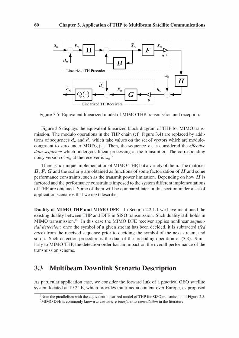
60 Chapter 3. Application of THP to Multibeam Satellite Communications
Figure 3.5: Equivalent linearized model of MIMO THP transmission and reception.
Figure 3.5 displays the equivalent linearized block diagram of THP for MIMO trans-
mission. The modulo operations in the THP chain (cf. Figure 3.4) are replaced by addi-
tions of sequences dn and dn which take values on the set of vectors which are modulo-
congruent to zero under MOD∆ (·). Then, the sequence vn is considered the effective
data sequence which undergoes linear processing at the transmitter. The corresponding
noisy version of vn at the receiver is zn.9
There is no unique implementation of MIMO-THP, but a variety of them. The matrices
B, F , G and the scalar g are obtained as functions of some factorization of H and some
performance constraints, such as the transmit power limitation. Depending on how H is
factored and the performance constraints imposed to the system different implementations
of THP are obtained. Some of them will be compared later in this section under a set of
application scenarios that we next describe.
Duality of MIMO THP and MIMO DFE In Section 2.2.1.1 we have mentioned the
existing duality between THP and DFE in SISO transmission. Such duality still holds in
MIMO transmission.10 In this case the MIMO DFE receiver applies nonlinear sequen-
tial detection: once the symbol of a given stream has been decided, it is subtracted (fed
back) from the received sequence prior to deciding the symbol of the next stream, and
so on. Such detection procedure is the dual of the precoding operation of (3.8). Simi-
larly to MIMO THP, the detection order has an impact on the overall performance of the
transmission scheme.
3.3 Multibeam Downlink Scenario Description
As particular application case, we consider the forward link of a practical GEO satellite
system located at 19.2◦ E, which provides multimedia content over Europe, as proposed
9Note the parallelism with the equivalent linearized model of THP for SISO transmission of Figure 2.5.10MIMO DFE is commonly known as successive interference cancellation in the literature.
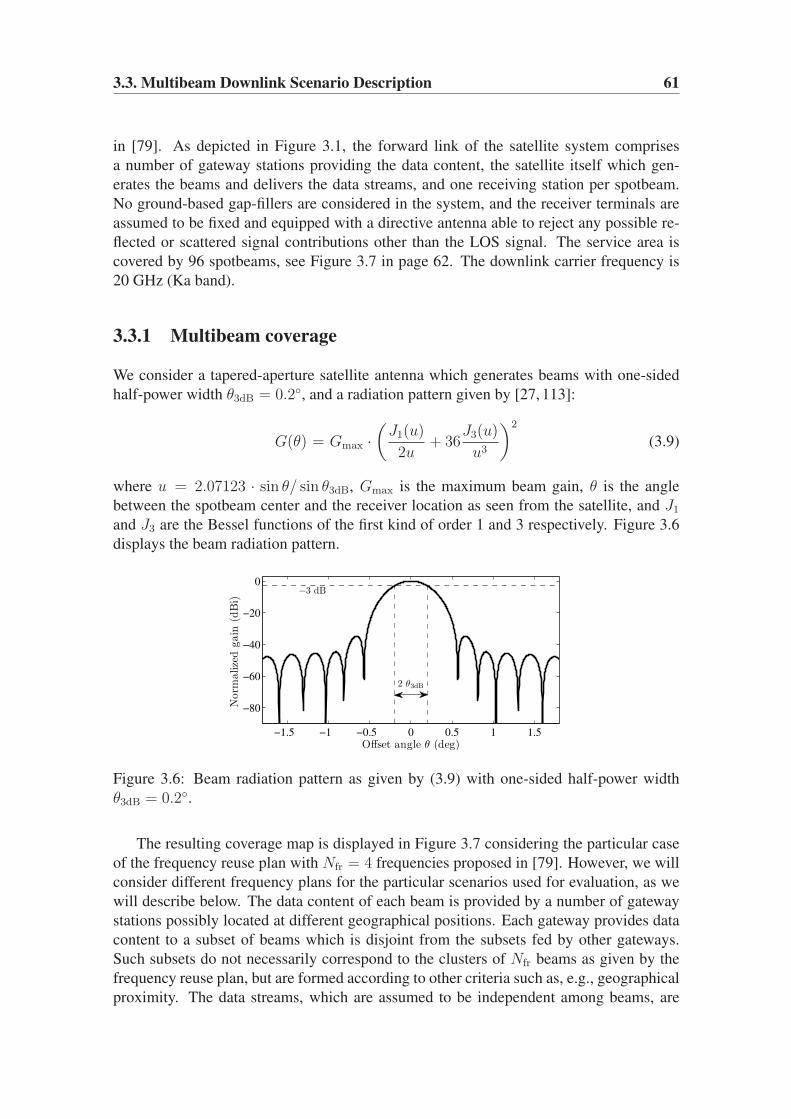
3.3. Multibeam Downlink Scenario Description 61
in [79]. As depicted in Figure 3.1, the forward link of the satellite system comprises
a number of gateway stations providing the data content, the satellite itself which gen-
erates the beams and delivers the data streams, and one receiving station per spotbeam.
No ground-based gap-fillers are considered in the system, and the receiver terminals are
assumed to be fixed and equipped with a directive antenna able to reject any possible re-
flected or scattered signal contributions other than the LOS signal. The service area is
covered by 96 spotbeams, see Figure 3.7 in page 62. The downlink carrier frequency is
20 GHz (Ka band).
3.3.1 Multibeam coverage
We consider a tapered-aperture satellite antenna which generates beams with one-sided
half-power width θ3dB = 0.2◦, and a radiation pattern given by [27, 113]:
G(θ) = Gmax ·(J1(u)
2u+ 36
J3(u)
u3
)2
(3.9)
where u = 2.07123 · sin θ/ sin θ3dB, Gmax is the maximum beam gain, θ is the angle
between the spotbeam center and the receiver location as seen from the satellite, and J1and J3 are the Bessel functions of the first kind of order 1 and 3 respectively. Figure 3.6
displays the beam radiation pattern.
−1.5 −1 −0.5 0 0.5 1 1.5
−80
−60
−40
−20
0−3 dB
2 θ3dB
Offset angle θ (deg)
Norm
alize
dgain
(dB
i)
Figure 3.6: Beam radiation pattern as given by (3.9) with one-sided half-power width
θ3dB = 0.2◦.
The resulting coverage map is displayed in Figure 3.7 considering the particular case
of the frequency reuse plan with Nfr = 4 frequencies proposed in [79]. However, we will
consider different frequency plans for the particular scenarios used for evaluation, as we
will describe below. The data content of each beam is provided by a number of gateway
stations possibly located at different geographical positions. Each gateway provides data
content to a subset of beams which is disjoint from the subsets fed by other gateways.
Such subsets do not necessarily correspond to the clusters of Nfr beams as given by the
frequency reuse plan, but are formed according to other criteria such as, e.g., geographical
proximity. The data streams, which are assumed to be independent among beams, are

62 Chapter 3. Application of THP to Multibeam Satellite Communications
Figure 3.7: Coverage and spotbeam distribution of the considered multibeam system with
a sample frequency reuse factor of Nfr = 4 frequencies (marked in different colors), as
proposed in [79].
multiplexed (e.g. in frequency and polarization) before being sent to the satellite through
the feeder link. At the satellite, the data streams from all gateways are demultiplexed and
distributed to the appropriate beams.
3.3.2 Satellite system details
Although the original system proposed in [79] considers a satellite with onboard pro-
cessing and switching capabilities, such assumption is not needed, so satellites with no
switching capabilities and with limited or no processing capabilities would be also valid
for implementation of the proposed system. When the satellite cannot perform onboard
processing we speak of a bent-pipe architecture in which the effect of the satellite is
transparent. Figure 3.8 displays the most representative blocks of a sample forward link
transmission chain, from the gateway to the receiving terminal. The block diagram is not
intended to include all stages of a real satellite system, but only those needed to justify our
signal model. The beamforming blocks represent the linear signal preprocessing stages
required to adapt the signals to be transmitted to the satellite antenna, so that the desired
multibeam radiation pattern is generated, and each beam carries the desired signals. The
beamforming task can be completely performed at the gateway or onboard the satellite,
or jointly at both places (for this reason there is a beamforming block at both places). The
choice between these alternatives depends on the processing capabilities of the payload
onboard. The beamforming stage is transparent from the receiver’s point of view, so it
will not be considered for the signal model. We refer to Appendix 3.C, where we provide
an overview of the different approaches to the beamforming task.
Regarding the rest of blocks, the next assumptions will be made in order to simplify

3.3. Multibeam Downlink Scenario Description 63
Figure 3.8: Block diagram of a multibeam satellite system (forward link) implementing
THP, including gateway, satellite and receivers. Dashed blocks might be implemented
either at the gateway or onboard. White blocks are “transparent” under our signal model
from the receivers’ point of view.
our analysis:
As3.1) Transparent IF and RF conversions. All frequency conversions in the chain are
ideal, i.e., they do not introduce any degradation in the transmitted signals.
As3.2) Transparent (de)multiplexing. The multiplexing at the gateway and the demul-
tiplexing onboard do not alter the transmitted signals.
As3.3) Perfect timing and carrier recovery. The receiver is assumed to implement
sufficiently accurate timing, phase and frequency acquisition schemes, so that they
do not impact negatively the received signal.
As3.4) Linear HPAs. The HPAs at the gateway and onboard the satellite are assumed to
operate under linear conditions, so that they do not introduce nonlinear distortion.
As3.5) Perfect CSI knowledge. The Channel State Information (CSI), i.e., the channel
response, is assumed to have a sufficiently slow variation (quasi-static channel) so
that some channel estimation procedure can perfectly estimate and track the chan-
nel state at any moment. The existence of an ideal return channel is furthermore
assumed so that the estimated CSI can be accurately passed back to the transmitter.
Perfect CSI knowledge is required for the proper application of THP transmission
as presented in Section 3.2.
The linear assumption for the gateway HPA is reasonable since simple countermea-
sures against nonlinear distortion can be employed in the gateway (e.g. a sufficient back-
off [39]) with low impact in the overall system cost. However, assuming a linear HPA
onboard seems unrealistic unless proper countermeasures such as predistortion are ap-
plied (large back-offs are prohibitive). Since our goal in this chapter is to evaluate the

64 Chapter 3. Application of THP to Multibeam Satellite Communications
system performance under ideal conditions, we will consider that such countermeasures
are applied. We note, however, that the application of predistortion in multibeam trans-
mission may not be as simple as in the case of SISO transmission seen in Section 2.3. We
refer to Appendix 3.D for a initial analysis on this issue.
Similarly, the perfect CSI knowledge assumption is motivated by the need of simplify-
ing the analysis as much as possible. In general, any channel estimation scheme will offer
imperfect estimates whose effect in the performance of THP must be properly considered.
We refer to Appendix 3.E where we provide an overview of the techniques available in
the literature for dealing with imperfect CSI.
Since the receivers are fixed terminals equipped with directive antennas, it can be con-
sidered that there is no multipath in the signals received at each terminal. Considering the
above assumptions, the narrowband signal model presented in Section 3.2.1 applies under
such quasi-static flat-fading conditions, with the (i, j) element of the channel matrix H ,
hij , representing the channel gain of the j-th beam towards the i-th receiver. In fact, the
value of the channel gain hij is a function of the radiation pattern (given by (3.9) and
assumed equal for all beams) and the relative position of the i-th receiver with respect to
the center of the j-th beam. The only source of interference are then the signals corre-
sponding to other beams reusing the same frequency (CCI), which partially reach outside
their spotbeams due to the sidelobes of the radiation pattern. As mentioned in Section 3.2,
from each receiver’s point of view such a communication scenario can be regarded as a
MISO scheme. On one side of the link, the gateway-satellite chain acts as a single trans-
mitter delivering a given number of simultaneous transmitted streams (beams). At the
other end, a terminal (one per spotbeam, and independent of other terminals) receives its
signal corrupted with AWGN and CCI from other beams reusing the same frequency.
3.3.3 Particular evaluation scenarios
For the sake of evaluation we have selected a set of sample scenarios based on the coverage
pattern of Figure 3.7. Each scenario exhibits different features so as to cover a meaningful
range of application examples. The varying features among the selected scenarios are (i)
the location of the receivers within their spotbeams, (ii) the frequency reuse factor, and
(iii) the total number of beams controlled by a single gateway (NB). This yields scenarios
with different levels of CCI and processing complexity. We have selected four scenarios,
which will be labeled as Si, with i = 1, 2, 3, 4. Figure 3.9 represents the spotbeams con-
sidered in each scenario and the location of the receivers. The beams marked in gray are
assumed to cause no interference. We refer to Appendix 3.B where we provide the details
on the geographical location of the spotbeam centers and the receivers for reproducibility
purposes. Next we provide a short description of each scenario:
S1) A gateway controls NB = 10 adjacent beams which reuse the same frequency.
Receivers are deliberately located near the beam borders, and very close to each
other, so that many of them will experience a high CCI level.
S2) The scenario is similar to S1, with a gateway controlling NB = 10 adjacent beams,
but with the receivers more sparsely located, which yields a moderate to high level
of CCI. Figure 3.10 displays the coverage map corresponding to this scenario.
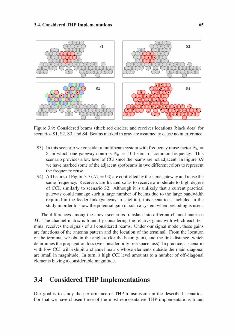
3.4. Considered THP Implementations 65
S1 S2
S3 S4
Figure 3.9: Considered beams (thick red circles) and receiver locations (black dots) for
scenarios S1, S2, S3, and S4. Beams marked in gray are assumed to cause no interference.
S3) In this scenario we consider a multibeam system with frequency reuse factor Nfr =3, in which one gateway controls NB = 10 beams of common frequency. This
scenario provides a low level of CCI since the beams are not adjacent. In Figure 3.9
we have marked some of the adjacent spotbeams in two different colors to represent
the frequency reuse.
S4) All beams of Figure 3.7 (NB = 96) are controlled by the same gateway and reuse the
same frequency. Receivers are located so as to receive a moderate to high degree
of CCI, similarly to scenario S2. Although it is unlikely that a current practical
gateway could manage such a large number of beams due to the large bandwidth
required in the feeder link (gateway to satellite), this scenario is included in the
study in order to show the potential gain of such a system when precoding is used.
The differences among the above scenarios translate into different channel matrices
H . The channel matrix is found by considering the relative gains with which each ter-
minal receives the signals of all considered beams. Under our signal model, these gains
are functions of the antenna pattern and the location of the terminal. From the location
of the terminal we obtain the angle θ (for the beam gain), and the link distance, which
determines the propagation loss (we consider only free space loss). In practice, a scenario
with low CCI will exhibit a channel matrix whose elements outside the main diagonal
are small in magnitude. In turn, a high CCI level amounts to a number of off-diagonal
elements having a considerable magnitude.
3.4 Considered THP Implementations
Our goal is to study the performance of THP transmission in the described scenarios.
For that we have chosen three of the most representative THP implementations found

66 Chapter 3. Application of THP to Multibeam Satellite Communications
Figure 3.10: Coverage map with the considered beams (marked in dark) and receiver
locations (marked with light squares) of scenario S2.
in the recent literature. Next we provide a description for which the block diagrams of
Figures 3.4 and 3.5 will be useful.
ZF-THP by Fischer et al., “ZF-THP-Fi”. We will consider the ZF solution proposed
by Fischer et al. in [60], and more detailed in [59]. In this scheme the channel matrix is
decomposed as
H = G−1ZF-Fi(I −BZF-Fi)F
HZF-Fi (3.10)
where F ZF-Fi is unitary. The diagonal matrix GZF-Fi and the feedback matrix BZF-Fi are
obtained through
R = G−1ZF-Fi(I −BZF-Fi) (3.11)
where R is a lower triangular matrix which can be obtained through the Cholesky factor-
ization
HHH = RRH. (3.12)
The diagonal matrix GZF-Fi does not present a constant diagonal in general, i.e., GZF-Fi 6=c · I . This implies that under this precoding scheme each receiver sees a different level of
SNR. Although no special ordering is considered in [59, 60], we will use the “best-first”
method to improve the performance of this scheme. In Section 3.A of the Appendix we
detail such ordering procedure.
THP by Joham et al., “ZF-THP-Jo” and “MMSE-THP-Jo”. We will also consider
the ZF and MMSE solutions proposed by Joham et al. in [97, 98]. These solutions are
obtained through minimization of Mean Square Error (MSE) between the transmitted and
received effective data sequences, E {‖vn − zn‖2}, under the ZF and MMSE criteria.

3.4. Considered THP Implementations 67
Assuming that a given permutation matrix Π is applied, the ZF solution can be obtained
via the Cholesky factorization
ΠHHHΠ
T = LLH (3.13)
with L lower triangular. Such decomposition allows to write the matrix filters and scaling
constant as follows
F ZF-Jo = HHΠ
T(LH)−1
D (3.14a)
BZF-Jo = I −LD (3.14b)
GZF-Jo = I (3.14c)
gZF-Jo =
√
E {‖xn‖2}ETX
(3.14d)
where E {‖xn‖2} is the average energy of the precoded sequence at the output of the
feedforward filter F (see Figure 3.3), and can be computed as
E{‖xn‖2
}= Tr (D2X) (3.15)
where D is a diagonal matrix whose diagonal elements are the inverses of those in the
diagonal of L, i.e., D.= diag
(([L]11)
−1, . . . , ([L]NBNB)−1). The matrix X in (3.14d) is
the covariance matrix of the sequence xn at the output of the modulo operator. Matrix
X can be considered diagonal since the modulo operation decorrelates the entries of xn.
We will assume that all precoded streams (entries) of xn have the same variance ∆2
6,
recall (2.11), except the one processed in the first place. Indeed, as indicated by (3.8a),
the first processed entry [Πa]1 remains unchanged, so the former variance does not apply.
Thus, X is a diagonal matrix with its nonzero entries given by
[X]ii.= σ2
[x]i=
{σ2a for i = 1
∆2
6otherwise.
(3.16)
Note that σ2a = 1, since we have assumed that the original constellation is normalized in
energy. Thus, it is possible to rewrite (3.15) as
E{‖xn‖2
}=
1
([L]11)2+
∆2
6
NB∑
i=2
1
([L]ii)2. (3.17)
As for the permutation matrix Π, it is obtained using “best-first” ordering. We refer to the
Section 3.A in the Appendix for the details.
Regarding the MMSE solution, unfortunately it is not possible to write it in terms
of some matrix factorization. Still, it is possible to write the solution in terms of the
feedforward matrix FMMSE-Jo as follows:
[BMMSE-Jo]ij =
{0 for i ≤ j−[ΠHFMMSE-Jo]ij for i > j
, 1 ≤ i, j ≤ NB (3.18a)
GMMSE-Jo = I (3.18b)
gMMSE-Jo =
√
E {‖xn‖2}ETX
(3.18c)

68 Chapter 3. Application of THP to Multibeam Satellite Communications
with ξ.= (NB ·σ2
w)/ETX, i.e., the ratio of aggregate received noise power to total transmit-
ted power. The permutation matrix Π is obtained using “best-first” ordering as detailed
in Section 3.A of the Appendix. The feedforward matrix FMMSE-Jo admits a closed form.
However, its mathematical expression is somewhat intricate, and requires some auxiliary
matrices which are also used in “best-first” ordering. Therefore, we provide the expres-
sion of FMMSE-Jo in Section 3.A of the Appendix.
The value of E {‖xn‖2} (the average energy at the output of F ) can be written in
terms of the feedforward matrix FMMSE-Jo as follows (f i represents the i-th column of
FMMSE-Jo)
E{‖xn‖2
}=
NB∑
i=1
σ2[x]i
‖f i‖2 = ‖f 1‖2 +∆2
6
NB∑
i=2
‖f i‖2 (3.19)
where we have used that σ2[x]1
= σ2a = 1.
We note that G = I in both ZF and MMSE solutions, and thus the SNR is equally
balanced among all receivers.
THP by Sanguinetti et al., “ZF-THP-Sa”. We have also considered the ZF solution
proposed by Sanguinetti et al. in [140]. This solution can be seen as a generalization of
ZF-THP-Jo, which allows the provision of different levels of Quality of Service (QoS)
(i.e., SNR) to each receiver. The different SNR levels are represented by a real-valued
diagonal matrix Λ = diag (λ1, . . . , λNB). The computation of the matrices B and F and
the gain g proceeds similarly to the “ZF-THP-Jo” case, but incorporating matrix Λ in the
proper place. Assume that Λ and the permutation matrix Π are given. Then, application
of Cholesky factorization to ΠH yields
ΠHHHΠ
T = LLH (3.20)
with L lower triangular. With this, the precoding system is determined by
F ZF-Sa = HHΠ
T(LH)−1
DΛ (3.21a)
BZF-Sa = I −Λ−1LDΛ (3.21b)
GZF-Sa = I (3.21c)
gZF-Sa =
√
E {‖xn‖2}ETX
(3.21d)
with the permutation matrix Π obtained through “best-first” ordering (see Section 3.A for
the details). The diagonal matrix D is defined similarly to the case “ZF-THP-Jo”, and
E {‖xn‖2} incorporates now the effect of the matrix Λ as follows
E{‖xn‖2
}=
(λ1
[L]11)
)2
+∆2
6
NB∑
i=2
(λi
[L]ii)
)2
(3.22)
where again the fact σ2[x]1
= 1 has been used.

3.5. Results and Discussion 69
The diagonal matrix Λ is thus a further design parameter suitable to be tuned accord-
ing to the desired SNR differentiation among receivers. Its effect on the received signals
is clearly seen analyzing the SNR experienced by each receiver. The SNR seen by the i-threceiver can be written as
SNRi = λ2i ·(
1
σ2w · g2ZF-Sa
)
, 1 ≤ i ≤ NB (3.23)
where the term inside brackets, which is directly proportional to ETX through (3.21d), is
common to all receivers. With this scheme, an appropriate choice of the matrix Λ allows
to obtain any set of relative SNRs among the different receivers.11 If Λ = λI is chosen for
some real-valued scalar λ (i.e., all users experience the same SNR), the resulting scheme
boils down to “ZF-THP-Jo”.
3.5 Results and Discussion
We have evaluated the performance of all proposed precoding schemes for all selected
scenarios. For a fair comparison, all schemes transmit the same power. Therefore, the
comparison is made in terms of uncoded BER vs. Eb/N0, where Eb is the average trans-
mitted (instead of the received) energy per bit and N0 is the one-sided noise power spectral
density.
Figures 3.11 and 3.12 show the performance of precoding in a scenario S1 (high level
of CCI) using QPSK and 16-QAM signaling respectively. Clearly, if no precoding is
used the performance is very poor, reaching a high BER floor already at very low SNRs.
The reason for this is that the CCI dominates over the noise, and the level of Signal-to-
Interference plus Noise Ratio (SINR) remains the same despite a decrease in the noise
power. LP schemes are seen to improve the performance, but, as expected, THP outper-
forms LP in the high SNR region due to the transmitted energy penalty of the LP (around
12 dB with respect to THP in both cases). Also as expected, MMSE approaches yield
better results than their ZF counterparts in the low SNR region, whereas the performances
of both approaches tend to converge as the SNR increases. In the QPSK case, it is remark-
able that MMSE-LP performs better than ZF-THP for SNRs below 15 dB. A similar effect
is observed also for 16-QAM, but in this case for SNRs below 10 dB. Finally, Figs. 3.11
and 3.12 confirm the equal performances of ZF-THP-Jo and ZF-THP-Sa when the same
SNR is provided to all receivers in the latter implementation. Therefore, we drop ZF-
THP-Sa from subsequent comparisons. Finally, it can be seen in both cases that LP and
THP offer the same performance at very low SNRs. This is in accordance with the results
in [94], where it is proved that no additional gain can be expected from DPC or any of its
suboptimum approximations in the low SNR region.
Figures 3.13, 3.14 and 3.15 show the same as Figure 3.12 but for scenarios S2, S3 and
S4 respectively. In Figures 3.13 and 3.15 (intermediate-to-high CCI) the results are similar
11We speak of relative SNRs because the absolute values are ultimately constrained by the transmit power
limitation ETX.

70 Chapter 3. Application of THP to Multibeam Satellite Communications
−5 0 5 10 15 20 25 30 35
10−4
10−3
10−2
10−1
100
Scenario S1 (10 ×10), QPSK
Eb/N0 (dB)
Unco
ded
BE
R
No PrecodingZF-LPMMSE-LPZF-THP-Fi ord.ZF-THP-JoZF-THP-SaMMSE-THP-Jo
Figure 3.11: Performance in terms of uncoded BER of all precoding schemes for S1 using
QPSK.
−5 0 5 10 15 20 25 30 35
10−4
10−3
10−2
10−1
100
Scenario 1 (10 ×10), 16-QAM
Eb/N0 (dB)
Unco
ded
BE
R
No PrecodingZF-LPMMSE-LPZF-THP-Fi ord.ZF-THP-JoMMSE-THP-JoZF-THP-Sa
Figure 3.12: Performance in terms of uncoded BER of all precoding schemes for S1 using
16-QAM.

3.5. Results and Discussion 71
−5 0 5 10 15 20 25 30 35
10−4
10−3
10−2
10−1
100
Scenario S2 (10 ×10), 16-QAM
Eb/N0 (dB)
Unco
ded
BE
R
No PrecodingZF-LPMMSE-LPZF-THP-Fi ord.ZF-THP-JoMMSE-THP-Jo
Figure 3.13: Performance in terms of uncoded BER for S2 using 16-QAM.
−5 0 5 10 15 20
10−4
10−3
10−2
10−1
100
Scenario S3 (10 ×10), 16-QAM
Eb/N0 (dB)
Unco
ded
BE
R
No Precoding
ZF-LP
MMSE-LP
ZF-THP-Fi ord.
ZF-THP-Jo
MMSE-THP-Jo
Figure 3.14: Performance in terms of uncoded BER of all precoding schemes for S3 using
16-QAM.
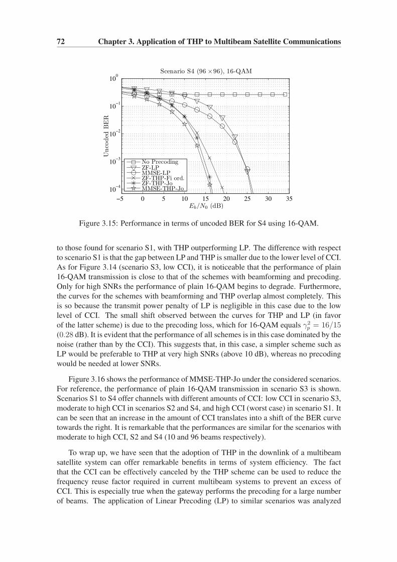
72 Chapter 3. Application of THP to Multibeam Satellite Communications
−5 0 5 10 15 20 25 30 35
10−4
10−3
10−2
10−1
100
Scenario S4 (96 ×96), 16-QAM
Eb/N0 (dB)
Unco
ded
BE
R
No PrecodingZF-LPMMSE-LPZF-THP-Fi ord.ZF-THP-JoMMSE-THP-Jo
Figure 3.15: Performance in terms of uncoded BER for S4 using 16-QAM.
to those found for scenario S1, with THP outperforming LP. The difference with respect
to scenario S1 is that the gap between LP and THP is smaller due to the lower level of CCI.
As for Figure 3.14 (scenario S3, low CCI), it is noticeable that the performance of plain
16-QAM transmission is close to that of the schemes with beamforming and precoding.
Only for high SNRs the performance of plain 16-QAM begins to degrade. Furthermore,
the curves for the schemes with beamforming and THP overlap almost completely. This
is so because the transmit power penalty of LP is negligible in this case due to the low
level of CCI. The small shift observed between the curves for THP and LP (in favor
of the latter scheme) is due to the precoding loss, which for 16-QAM equals γ2p = 16/15
(0.28 dB). It is evident that the performance of all schemes is in this case dominated by the
noise (rather than by the CCI). This suggests that, in this case, a simpler scheme such as
LP would be preferable to THP at very high SNRs (above 10 dB), whereas no precoding
would be needed at lower SNRs.
Figure 3.16 shows the performance of MMSE-THP-Jo under the considered scenarios.
For reference, the performance of plain 16-QAM transmission in scenario S3 is shown.
Scenarios S1 to S4 offer channels with different amounts of CCI: low CCI in scenario S3,
moderate to high CCI in scenarios S2 and S4, and high CCI (worst case) in scenario S1. It
can be seen that an increase in the amount of CCI translates into a shift of the BER curve
towards the right. It is remarkable that the performances are similar for the scenarios with
moderate to high CCI, S2 and S4 (10 and 96 beams respectively).
To wrap up, we have seen that the adoption of THP in the downlink of a multibeam
satellite system can offer remarkable benefits in terms of system efficiency. The fact
that the CCI can be effectively canceled by the THP scheme can be used to reduce the
frequency reuse factor required in current multibeam systems to prevent an excess of
CCI. This is especially true when the gateway performs the precoding for a large number
of beams. The application of Linear Precoding (LP) to similar scenarios was analyzed

3.5. Results and Discussion 73
−5 0 5 10 15 20 25
10−4
10−3
10−2
10−1
100
MMSE-THP-Jo in S1, S2, S3, S4, 16-QAM
Eb/N0 (dB)
Unco
ded
BE
R
MMSE-THP-Jo S1 (10×10)MMSE-THP-Jo S2 (10×10)MMSE-THP-Jo S3 (10×10)No Precoding S3 (10×10)MMSE-THP-Jo S4 (96×96)
Figure 3.16: Performance in terms of uncoded BER of MMSE-THP-Jo for all scenarios
using 16-QAM.
in detail in [43, 67] offering interesting potential improvements in terms of throughput
with respect to traditional systems (above 80%). Our simulations show that even greater
improvements can be expected if THP is used, mainly due to the removal of the transmit
power penalty inherent to LP schemes.

74 Chapter 3. Application of THP to Multibeam Satellite Communications
Appendix 3.A Filter Computation for MIMO THP
3.A.1 “Best-first” Ordering
As mentioned in Section 3.2, the overall performance of MIMO precoding depends on the
particular precoding order. Recall that the precoding operation is performed sequentially,
as indicated in (3.8a)–(3.8c). Following the work in [97, 98], as optimality criterion we
consider the minimization of the MSE between the transmitted and received effective data
sequences. In reality, the optimal precoding order can only be determined by extensive
search. It would be necessary to test all of the NB! possible orderings and then choose
the one yielding the minimum MSE. Such task is computationally intensive, so some
suboptimal but feasible procedure would be desirable. One such scheme is the “best first”
ordering procedure, which is simpler but yields orderings which usually perform close to
optimality.
We note that in all precoding schemes proposed in Section 3.4, matrices B and F ,
and the scaling constant g depend on the permutation matrix Π. Therefore, the precoding
order must in general be found in the first place, and then proceed to the computation of
the matrices and the constant. It is possible, however, to jointly compute the columns of
Π and F , by applying a sequential algorithm as detailed in [97, 98], although we will not
provide the details here.
We describe next how best-first ordering works following [97,98]. The basic principle
is to minimize the MSE between the NB received and transmitted effective data sequences.
Each MSE is minimized assuming a fixed ordering of the streams to be precoded next.
Depending on the precoding scheme (ZF or MMSE), the ordering procedure changes.
Omitting the details (see [97, 98] for the derivation), the ordering procedure is as follows
(O(·) represents the set of ordered indices):
OZF = {o1, o2, . . . , oNB} with
oi = argmino ∈{1,...,NB}\{oi+1,...,oNB
}
[ΠiHHH
Πi
]+
oofor i = NB, . . . , 1 (3.24)
for ZF-THP, and
OMMSE = {o1, o2, . . . , oNB} with
oi = argmino ∈{1,...,NB}\{oi+1,...,oNB
}
[ΠiHHH
Πi + ξI]−1
oofor i = NB, . . . , 1 (3.25)
for MMSE-THP, with ξ.= NB·σ2
w
ETX. In both cases, the projection matrices Πi are diagonal
matrices which, given a precoding order O = {o1, o2, . . . , oNB}, are defined as
ΠNB= I, (3.26a)
[Πi]kk =
{0 if k = oi[Πi+1]kk otherwise
, for i = NB − 1, . . . , 1. (3.26b)
The permutation matrix Π is then a pure function of the obtained ordering, OZF or OMMSE.

3.B. Receiver Locations for Scenarios S1, S2 and S3 75
Procedure (3.24) is valid for all the proposed ZF schemes: “ZF-THP-Fi”, “ZF-THP-
Jo”, and “ZF-THP-Sa”. In the latter case, the only change is that the modified matrix
Λ−1H must be used instead of H .
Note that in procedures (3.24) and (3.25) the first obtained index refers to the data
stream to be precoded in the last place, followed by the second last, and so on until the
index of the stream to be precoded first, which is obtained in the last place.
3.A.2 Feedforward Matrix Computation for “MMSE-THP-Jo”
In Section 3.4 we indicate the solution to the “MMSE-THP-Jo” case as a function of
the feedforward matrix FMMSE-Jo, which is not provided. Here we provide its closed
form expression, for which we will take advantage of the projection matrices Πi, already
defined by (3.26). Instead of a single expression for FMMSE-Jo, it is more convenient to
provide the expression of its columns. By f i we will denote the i-th column of FMMSE-Jo,
and we will assume that the precoding order has already been found and is given by
O = {o1, o2, . . . , oNB}. We introduce the matrix
A(i) .= HH
Πi(ΠiHHHΠi + ξI)−1 (3.27)
with ξ = NB·σ2w
ETX, and whose j-th column we denote by a
(i)j , i.e.,
A(i) = [a(i)1 ,a
(i)2 , . . . ,a
(i)NB].
Then FMMSE-Jo is defined columnwise as follows
FMMSE-Jo = [f 1,f 2, . . . ,fNB] with (3.28a)
f i = a(i)oi, 1 ≤ i ≤ NB (3.28b)
i.e., the i-th column of FMMSE-Jo is given by the oi-th column of A(i). Note that the
computation of each column of FMMSE-Jo requires the computation of a different matrix
A(i).
Appendix 3.B Receiver Locations for Scenarios S1, S2 and
S3
For the sake of reproducibility, we include in this appendix the coordinates of the 96
spotbeam centers of the multibeam system detailed in Section 3.3 (see Figure 3.7). We
also provide the receiver locations for scenarios S1, S2 and S3 (see Figure 3.9). Scenario
S4 is left out for economy of space.
Table 3.1 lists the coordinates of the 96 spotbeam centers. The spotbeams are num-
bered from 1 to 96, from West to East and North to South. For example, the spotbeams in
the most northern row are numbered from 1 to 4; those in the second most northern row
are numbered from 5 to 10, and so on. Tables 3.2 provides the coordinates of the receiver
locations for scenarios S1, S2 and S3. We include in the table the index of the spotbeam
which the receiver belongs to.

76 Chapter 3. Application of THP to Multibeam Satellite Communications
Table 3.1: Location of the spotbeam centers considered in Section 3.3. Spotbeams are
numbered from 1 to 96. Partial horizontal lines indicate where a new row of spotbeams
starts.
Nr. Center location Nr. Center location Nr. Center location
1 67.00◦N 11.00◦E 33 48.75◦N 11.90◦E 65 39.75◦N 1.50◦W
2 67.00◦N 16.25◦E 34 48.75◦N 14.80◦E 66 39.75◦N 0.75◦E
3 67.00◦N 21.75◦E 35 48.75◦N 17.80◦E 67 39.75◦N 3.50◦E
4 67.00◦N 27.50◦E 36 48.75◦N 21.00◦E 68 39.75◦N 9.25◦E
5 61.00◦N 6.50◦E 37 45.50◦N 0.90◦W 69 39.75◦N 14.50◦E
6 61.00◦N 10.75◦E 38 45.50◦N 2.00◦E 70 39.75◦N 17.00◦E
7 61.00◦N 15.00◦E 39 45.50◦N 4.80◦E 71 39.75◦N 19.50◦E
8 61.00◦N 19.25◦E 40 45.50◦N 7.80◦E 72 39.75◦N 21.75◦E
9 61.00◦N 23.50◦E 41 45.50◦N 10.80◦E 73 39.75◦N 24.00◦E
10 61.00◦N 27.75◦E 42 45.50◦N 13.70◦E 74 39.75◦N 26.50◦E
11 56.20◦N 6.25◦W 43 45.50◦N 16.50◦E 75 39.75◦N 29.25◦E
12 56.20◦N 2.00◦W 44 45.50◦N 19.30◦E 76 39.75◦N 32.00◦E
13 56.20◦N 10.00◦E 45 45.50◦N 22.10◦E 77 39.75◦N 34.75◦E
14 56.20◦N 13.75◦E 46 42.25◦N 7.25◦W 78 39.75◦N 37.50◦E
15 56.20◦N 17.50◦E 47 42.50◦N 4.25◦W 79 39.75◦N 40.25◦E
16 56.20◦N 21.25◦E 48 42.50◦N 1.25◦W 80 39.75◦N 43.20◦E
17 56.20◦N 25.00◦E 49 42.50◦N 1.50◦E 81 37.75◦N 7.75◦W
18 52.25◦N 8.90◦W 50 42.50◦N 4.25◦E 82 37.25◦N 5.00◦W
19 52.25◦N 5.65◦W 51 42.50◦N 7.25◦E 83 37.25◦N 2.00◦W
20 52.25◦N 1.85◦W 52 42.50◦N 10.00◦E 84 37.25◦N 13.50◦E
21 52.00◦N 2.20◦E 53 42.50◦N 12.75◦E 85 37.25◦N 16.00◦E
22 52.25◦N 5.75◦E 54 42.50◦N 15.50◦E 86 37.25◦N 22.75◦E
23 52.25◦N 9.25◦E 55 42.50◦N 18.25◦E 87 37.25◦N 25.00◦E
24 52.25◦N 12.75◦E 56 42.50◦N 20.75◦E 88 37.25◦N 27.50◦E
25 52.25◦N 16.00◦E 57 42.50◦N 23.25◦E 89 37.25◦N 30.25◦E
26 52.25◦N 19.25◦E 58 42.50◦N 25.75◦E 90 37.25◦N 32.75◦E
27 52.25◦N 22.50◦E 59 42.50◦N 28.50◦E 91 37.25◦N 35.50◦E
28 48.75◦N 4.00◦W 60 42.50◦N 31.25◦E 92 37.25◦N 38.00◦E
29 48.75◦N 1.25◦W 61 42.50◦N 34.25◦E 93 37.25◦N 40.75◦E
30 48.75◦N 2.00◦E 62 42.50◦N 37.00◦E 94 37.25◦N 43.50◦E
31 48.75◦N 5.40◦E 63 39.90◦N 7.50◦W 95 35.00◦N 25.00◦E
32 48.75◦N 8.75◦E 64 39.75◦N 4.25◦W 96 35.00◦N 33.50◦E

3.C. Beamforming Implementation 77
Table 3.2: Receiver locations for scenarios S1, S2 and S3. “SB Nr.” stands for the re-
ceiver’s spotbeam number, as listed in Table 3.1.
S1 S2 S3
SB Nr. Receiver location SB Nr. Receiver location SB Nr. Receiver location
22 51.00◦N 7.00◦E 21 50.20◦N 2.25◦E 7 63.00◦N 12.50◦E
23 51.00◦N 11.00◦E 22 53.50◦N 6.00◦E 10 61.00◦N 30.00◦E
24 51.00◦N 11.50◦E 23 52.00◦N 8.00◦E 12 58.50◦N 3.00◦W
25 51.00◦N 14.50◦E 30 50.00◦N 1.00◦E 13 56.60◦N 11.00◦E
32 50.50◦N 9.00◦E 31 48.75◦N 7.00◦E 16 56.40◦N 20.20◦E
33 50.50◦N 11.90◦E 32 49.50◦N 10.00◦E 19 54.00◦N 6.50◦W
34 50.50◦N 15.00◦E 33 48.50◦N 12.50◦E 22 52.50◦N 5.10◦W
35 50.50◦N 16.00◦E 39 45.00◦N 6.50◦E 25 51.00◦N 17.30◦E
41 46.75◦N 11.80◦E 40 44.50◦N 9.25◦E 30 49.50◦N 2.50◦E
42 46.75◦N 12.70◦E 41 44.50◦N 11.50◦E 33 50.00◦N 12.50◦E
Appendix 3.C Beamforming Implementation
An important issue not addressed in the main text of this chapter is the implementation
of the antenna beamforming. By beamforming we refer to the techniques used to shape
the radiation pattern of the satellite antenna so that the coverage area is illuminated as
desired. We provide here a brief overview of the state-of-the-art antenna technology and
beam conformation techniques, and their possible relationship with the precoding stage.
Typically, a GEO satellite broadcasting TV over a region implements a single beam.
The shape of the beam is adapted to the region of coverage with some kind of beamform-
ing technology in order not to waste transmission power over undesired regions such as
oceans. In contrast, in multibeam systems the desired coverage is achieved through the
superposition of a number of smaller beams of circular or elliptical shape. In principle,
each of these beams can be fed with a signal which is completely independent of the sig-
nals from the rest of beams. This fact is exploited in the THP-based transmission system
considered in this chapter.
Figure 3.17: Simplified block diagram of a multibeam transmission scheme using THP.
In general, beam conformation is achieved in two steps, as illustrated in Figure 3.17.
The eventual radiation pattern is determined by the combined action of the former stages:
• First, the beamforming stage is a signal preprocessing block which adapts the sig-
nals to be transmitted (say NB beam signals) to the Nf antenna feed. This prepro-
cessing stage has been traditionally implemented in the analog domain, although
digital processing techniques are possible and may be considered for future sys-
tems. The beamforming stage has been typically located onboard the satellite, al-

78 Chapter 3. Application of THP to Multibeam Satellite Communications
though several systems have been recently proposed or implemented in which the
preprocessing is (at least partially) performed on ground, as we will see below.
• The satellite antenna is the last stage before the signals exit the satellite. By an-
tenna we refer to both the feeds and the possible reflector.
Multibeam Antenna Technologies We briefly provide a classification of the satellite
antenna systems suitable to implement multibeam coverage. Four main possibilities ex-
ist [108, 116]:
• Single Reflector Feed (SRF) system. It consists of one reflector which is illumi-
nated by a feed array, with each feed generating a constituent beam. Actual beams
are formed by superposition of several constituent beams.
• Single Reflector with Hybrid Transform (SRHT) system. It is basically an SRF
system in which an hybrid transformer or a Butler matrix12 is placed directly before
the feeds with the purpose of distributing the energy evenly among the feeds.
• Dual Reflector Array-Fed (DRAF) system. This system uses a smaller subreflec-
tor located between the feeds and the main reflector. The subreflector produces an
extra signal transformation which yields a uniform amplitude output.
• Directly Radiating Array (DRA) system. No reflector is used under this configu-
ration, so the antenna elements radiate directly towards the coverage region on the
Earth surface. The size of the array must be comparable to that of the main reflec-
tors of the above configurations. Depending on the total power to be radiated, an
active amplifier module must be connected to each single feed or to a small group
of them.
Roughly speaking, the number of feeds is proportional to the number of beams to be
deployed. Current multibeam systems deploy antennas with more than one hundred
feeds [44, 61, 156]
Beamforming schemes The task of the beamforming stage is to provide the adequate
signals to the antenna feeds so that the desired beams are formed. In general, the number
of beams NB will not coincide with the number of the antenna feeds (Nf). Thus, the pre-
processing stage must apply some kind of combination of its inputs, implicitly performing
a dimensional transformation from NB to Nf. The beamforming operation amounts to a
weighted linear combination of the input signals, so that it can be represented using ma-
trix notation. Figure 3.18 shows this, representing the beamforming operation through the
Nf × NB matrix MBF, and the joint effect of antenna and propagation by means of the
NB × Nf matrix H rad. The cascade of MBF and H rad amounts to the channel matrix H
considered in the signal model of Section 3.2.1, i.e., H = H rad ·MBF.
Beamforming techniques, originally performed in the analog domain, evolved signif-
icantly with the application of digital processing techniques. In practice both approaches
can be used together, but it is the digital part which provides a degree of flexibility un-
reachable by pure analog beamforming. Whereas analog beamforming can take place at
12Butler matrices are analog beamforming networks whose processing is equivalent to that of a Fast
Fourier Transform (FFT), but performed in the analog domain.
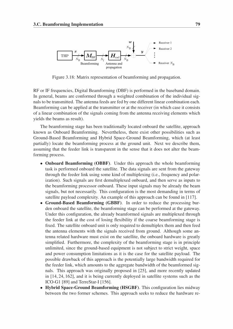
3.C. Beamforming Implementation 79
Figure 3.18: Matrix representation of beamforming and propagation.
RF or IF frequencies, Digital Beamforming (DBF) is performed in the baseband domain.
In general, beams are conformed through a weighted combination of the individual sig-
nals to be transmitted. The antenna feeds are fed by one different linear combination each.
Beamforming can be applied at the transmitter or at the receiver (in which case it consists
of a linear combination of the signals coming from the antenna receiving elements which
yields the beams as result).
The beamforming stage has been traditionally located onboard the satellite, approach
known as Onboard Beamforming. Nevertheless, there exist other possibilities such as
Ground-Based Beamforming and Hybrid Space-Ground Beamforming, which (at least
partially) locate the beamforming process at the ground unit. Next we describe them,
assuming that the feeder link is transparent in the sense that it does not alter the beam-
forming process.
• Onboard Beamforming (OBBF). Under this approach the whole beamforming
task is performed onboard the satellite. The data signals are sent from the gateway
through the feeder link using some kind of multiplexing (i.e., frequency and polar-
ization). Such signals are first demultiplexed onboard, and then serve as inputs to
the beamforming processor onboard. These input signals may be already the beam
signals, but not necessarily. This configuration is the most demanding in terms of
satellite payload complexity. An example of this approach can be found in [117].
• Ground-Based Beamforming (GBBF). In order to reduce the processing bur-
den onboard the satellite, the beamforming stage can be performed at the gateway.
Under this configuration, the already beamformed signals are multiplexed through
the feeder link at the cost of losing flexibility if the coarse beamforming stage is
fixed. The satellite onboard unit is only required to demultiplex them and then feed
the antenna elements with the signals received from ground. Although some an-
tenna related hardware must exist on the satellite, the onboard hardware is greatly
simplified. Furthermore, the complexity of the beamforming stage is in principle
unlimited, since the ground-based equipment is not subject to strict weight, space
and power consumption limitations as it is the case for the satellite payload. The
possible drawback of this approach is the potentially large bandwidth required for
the feeder link, which amounts to the aggregate bandwidth of the beamformed sig-
nals. This approach was originally proposed in [25], and more recently updated
in [14, 24, 162], and it is being currently deployed in satellite systems such as the
ICO-G1 [89] and TerreStar-I [156].
• Hybrid Space-Ground Beamforming (HSGBF). This configuration lies midway
between the two former schemes. This approach seeks to reduce the hardware re-

80 Chapter 3. Application of THP to Multibeam Satellite Communications
quirements onboard the satellite with respect to the OBBF approach, and simultane-
ously reduce the bandwidth required for the feeder link with respect to the GBBF
scheme. The beamforming task is divided between the gateway and the satellite
payload. The gateway performs most of the beamforming process, and the task is
completed by an onboard unit with “coarse” beamforming capabilities (e.g., an FFT
matrix). By doing this it is possible to reduce the number of signals sent through
the feeder link. This beamforming scheme has been proposed in [13, 134].
As already mentioned, a THP system with one receiver per beam such as that con-
sidered in this chapter apparently calls for the use of beam-space beamforming, since the
precoding operation already provides one separate data stream per beam. A key issue for
the correct performance of the THP multibeam system is the minimization of the impact
of the nonlinear elements of the transmission chain, including the gateway and the satel-
lite. Among possible sources of nonlinear distortion are frequency mismatches in RF and
IF mixers, signal couplings, and the nonlinear characteristics of the gateway and onboard
HPAs. The possible effects of the HPA-induced nonlinearities are dealt with in the next
section. In general, the presence of nonlinearities will entangle the signals intended to
different users, and therefore will harm the performance of the precoding scheme.
Appendix 3.D Nonlinear Distortion in the Multibeam Down-
link Scenario
In this section we focus on the multibeam downlink scenario since the compensation of the
satellite HPA nonlinearity via predistortion for the SISO case was analyzed in Chapter 2.
The baud rate signal model assumed in Section 3.2 for the proposed precoded system
(see Figure 3.4) does not consider the nonlinear effects that the HPAs may introduce in
the transmission chain. If such nonlinearities are disregarded, then the chain gateway-
satellite-receiver is linear, so that the channel matrix H includes the combined effects of
the beamforming stage onboard, antenna and propagation. However, if nonlinearities can-
not be neglected then the linear model is insufficient. The aim of this section is to provide
a brief analysis of the effects of the HPA nonlinearity within the multibeam precoding
setup. Only the effect of the satellite HPA is considered. The HPA at the gateway is as-
sumed to introduce negligible nonlinear distortion, assuming that proper countermeasures
are employed in the gateway (e.g. back-off [39]), and the RF up- and down-converters at
the gateway, satellite and receivers are supposed to introduce no further distortion.
Figure 3.19 represents the resulting block diagram of the system including THP, beam-
forming and HPA onboard. The RF upconversion block represent the corresponding op-
eration performed e.g. at the gateway, but we assume they work ideally. Its inclusion in
Figure 3.19 is to indicate where the limits lie between baseband and RF processing. The
HPA block represents in fact one HPA per antenna feed.13 We will assume that the HPAs
13This model is in principle valid even when multiport amplifiers are used. Multiport amplifiers [53,115,
154] are composed of a number (usually a power of two) of SSPAs working in parallel and two RF mixing
matrices (e.g., analog Butler matrices) of the same dimension located at the input and the output of the

3.D. Nonlinear Distortion in the Multibeam Downlink Scenario 81
Figure 3.19: Simplified block diagram of the transmission chain including THP, beam-
forming and HPA onboard.
do not introduce “cross-talk”, i.e., no fraction of their input signals is driven into any feed
other than the correct one.
The main issue observed in Figure 3.19 is that the nonlinear HPAs are located be-
tween two linear blocks. If we assume ideal (linear) amplifier behavior, then the HPA
block becomes transparent, and the cascade of beamforming and propagation matrices
behaves as a single channel matrix H = H rad · MBF, which corresponds in fact with
the channel matrix H of the signal model considered in Section 3.2.1. However, when
the HPA behavior departs from linearity this simplified model does not apply anymore.
The main consequence of the presence of the HPAs between the two linear blocks is that
each beam signal is not only affected by self-induced nonlinear distortion but also from
(nonlinear) contributions from signals belonging to other beams (nonlinear interbeam in-
terference), including cross terms between signals belonging to different beams. This is
due to the beamforming stage, represented by MBF, whose effect is to spread the beam
signals among all feeds. Therefore, if the HPA associated to one feed introduces nonlinear
distortion, such distortion will be affecting the signals corresponding to all beams.
The question that arises now is: Is it possible to achieve nonlinear interference-free
transmission (including interbeam contributions) in a multibeam satellite system using
THP while maintaining non-cooperativeness among receivers?
To the best of the author’s knowledge, this specific topic does not seem to have been
addressed in the open literature. Possible solutions must necessarily consider system-
specific features such as the employed beamforming scheme, the particular satellite HPA
models and the possibility of applying adequate processing onboard the satellite, which
may not be guaranteed depending on the affordable or already onboard located payload.
We leave the actual solution here as a future research line, although in the remainder of
this section we will provide a shallow overview of different possible approaches to the
solution.
3.D.1 Possible Approaches to Predistortion
Initially we can consider solutions based on applying some processing either at transmitter
side (predistortion) or at receiver side (postdistortion), or at both locations. However, the
amplifiers. The output matrix is placed immediately before the feeds. The effect of the input and output
matrices could be properly accounted for within, respectively, the matrices MBF and H rad of Figure 3.19.
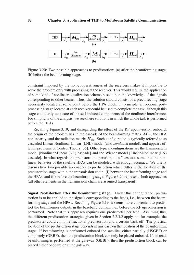
82 Chapter 3. Application of THP to Multibeam Satellite Communications
Figure 3.20: Two possible approaches to predistortion: (a) after the beamforming stage,
(b) before the beamforming stage.
constraint imposed by the non-cooperativeness of the receivers makes it impossible to
solve the problem only with processing at the receiver. This would require the application
of some kind of nonlinear equalization scheme based upon the knowledge of the signals
corresponding to other beams. Thus, the solution should consist of a precorrecting stage
necessarily located at some point before the HPA block. In principle, an optional post-
processing stage located at each receiver could be used to complete the task, although this
stage could only take care of the self-induced components of the nonlinear interference.
For simplicity of the analysis, we seek here solutions in which the whole task is performed
before the HPAs.
Recalling Figure 3.19, and disregarding the effect of the RF upconversion onboard,
the origin of the problem lies in the cascade of the beamforming matrix MBF, the HPA
nonlinearity, and the radiation matrix H rad. Such configuration is typically referred to as
cascaded Linear-Nonlinear-Linear (LNL) model (also sandwich model), and appears of-
ten in problems of Control Theory [35]. Other typical configurations are the Hammerstein
model [Nonlinear-Linear (NL) cascade] and the Wiener model [Linear-Nonlinear (LN)
cascade]. In what regards the predistortion operation, it suffices to assume that the non-
linear behavior of the satellite HPAs can be modeled with enough accuracy. We briefly
discuss here two possible approaches to predistortion which differ in the location of the
predistortion stage within the transmission chain: (i) between the beamforming stage and
the HPAs, and (ii) before the beamforming stage. Figure 3.20 represents both approaches
(all other elements in the transmission chain are assumed transparent).
Signal Predistortion after the beamforming stage. Under this configuration, predis-
tortion is to be applied to the signals corresponding to the feeds, i.e., between the beam-
forming stage and the HPAs. Recalling Figure 3.19, it seems more convenient to predis-
tort the beamformer outputs in the baseband domain, i.e., before the RF upconversion is
performed. Note that this approach requires one predistorter per feed. Assuming this,
the different predistortion strategies given in Section 2.2.3.2 apply, so, for example, the
predistorter could combine fractional predistortion and a certain back-off. The physical
location of the predistortion stage depends in any case on the location of the beamforming
stage. If beamforming is performed onboard the satellite, either partially (HSGBF) or
completely (OBBF), then the predistortion block can only be placed onboard. If, instead,
beamforming is performed at the gateway (GBBF), then the predistortion block can be
placed either onboard or at the gateway.

3.E. CSI Knowledge 83
The possibility of performing the predistortion at the gateway is quite appealing, con-
sidering the presumably large number of signals to be predistorted (typically in the order
of one hundred, according to the current antenna technology). Indeed, gateway-based
predistortion has the advantages of adding no extra processing requirements to the satel-
lite payload, and, simultaneously, allowing the implementation of advanced predistortion
techniques (thanks to the larger processing capacity at the gateway), which would not be
affordable onboard. When performed at the gateway, the baseband beamformed signals
should be predistorted before being RF upconverted and multiplexed in frequency and
polarization for the feeder link.
Signal predistortion before the beamforming stage. An alternative to the above scheme
is to perform predistortion before the beamforming operation. Under this configuration
the predistortion stage would be preferably located at the gateway, irrespective of where
the beamforming task is performed. This scheme would be useful in the case that OBBF
or HSGBF are used, and there is no possibility of locating the predistortion stage onboard
the satellite. Basically, the problem here is how to precompensate (invert) a nonlinearity
that appears after a linear block (matrix MBF).
Tentatively, one could think of building the predistorter as an LNL cascade composed
of MBF, a nonlinear mapping inverting the HPA characteristic, and a matrix M+,rBF repre-
senting the right pseudoinverse of MBF. We note however that MBF is typically a “tall”
matrix, i.e., it has more rows than columns, since the number of feeds is typically larger
than the number of data streams, and therefore MBF does have a left pseudoinverse but not
a right pseudoinverse.14 In general, the precorrection of the nonlinearity in a LN cascade
seems quite a challenging problem, which may compromise this predistortion approach.
Appendix 3.E CSI Knowledge
Throughout Chapters 2 and 3 we have assumed a precise knowledge of the CSI at the
transmitter. In the SISO THP setup of Chapter 2 this translates into precise knowledge of
the channel response HC(f) (see Figure 2.11), and therefore of the discrete-time equiva-
lent transfer function H(z). As for the multibeam THP setup of Chapter 3 (see Figure 3.4),
full CSI knowledge amounts to perfect knowledge of the channel matrix H . Such assump-
tion allows to identify the performance of the proposed schemes under ideal conditions.
Nevertheless, perfect acquisition of the CSI may not be possible in many cases. In this
section we briefly describe possible techniques of channel estimation for both cases, and
review how THP can be applied when only partial CSI is available.
The performance of precoded transmission when there are inaccuracies in the channel
estimate has been studied e.g. in [150] (time-dispersive SISO THP) and [127] (MIMO
case). The performance degrades consistently with the degree of mismatch between the
estimated and the actual channel. The mismatches between true and estimated CSI can
14In other words, when MBF is “tall” it is possible to find a matrix M+BF (left pseudoinverse) such that
M+BF ·MBF = I , but not a matrix M
+,rBF such that MBF ·M+,r
BF = I .
84 Chapter 3. Application of THP to Multibeam Satellite Communications
be due to estimation and quantization errors, or time variations of the channel response.
Channel estimation for both SISO and MISO setups must necessarily consider the use
of DA schemes (e.g., pilot symbols or training sequences) to be used (at least) in the
initialization phase of the transmission. This startup phase, during which THP cannot be
yet applied, can be used to perform other tasks simultaneously, such as timing recovery
or frame acquisition. In addition, a complementary calibration scheme will be required
to aid in the frequency recovery, phase recovery and gain control tasks. Such calibration
scheme would be useful not only for channel estimation but also for the beamforming task.
Examples of calibration schemes adequate for these purposes can be found in [24, 162].
In the SISO case, if the transmission can be considered reciprocal (i.e., both trans-
mission ends perceive the same channel channel response), channel estimation may be
performed at one end, and then fed back to the other end. In this case, errors in the feed-
back transmission or in the quantization of the channel response may introduce degrada-
tion in the channel estimate, and should be taken into account. As a practical example,
the 10GBASE-T standard [90] establishes a transmission startup phase during which both
transmission ends exchange their channel estimates in the form of quantized taps.
Apart from the channel estimation required for the transmission start, some channel
tracking scheme may be required in cases where the channel response varies with time.
In this case, the channel estimates must be regularly updated by some channel tracking
scheme which should incorporate as much useful information as possible, including the
statistics of the channel coefficients and their variation. If the channel presents sufficiently
fast variations, the tracking scheme may not be able to track such variations, and precoding
may eventually fail. For this reason the application of THP transmission towards mobile
receivers is in principle compromised.
Considering the CSI uncertainty caused by the quantized, possibly delayed feedback,
several authors have proposed different precoding schemes designed to work under a cer-
tain degree of channel uncertainty (partial CSI knowledge), which exploit the statistical
knowledge of the channel variations to improve the performance of classical. Examples
of such schemes can be found in [37, 107] for the SISO setup, and [33, 34, 49, 87, 95] for
the MIMO setup.

Chapter 4SNR Estimation
Contents
4.1 Introduction . . . . . . . . . . . . . . . . . . . . . . . . . . . . . . . 86
4.2 Review of SNR Estimators . . . . . . . . . . . . . . . . . . . . . . . 88
4.2.1 Cramer-Rao Bounds for SNR Estimation . . . . . . . . . . . . 89
4.3 Higher-Order-Statistics-Based Non-Data-Aided SNR Estimation . . 90
4.3.1 Motivation and Section Outline . . . . . . . . . . . . . . . . . 90
4.3.2 A New Moments-Based Estimator . . . . . . . . . . . . . . . . 92
4.3.3 Statistical Analysis . . . . . . . . . . . . . . . . . . . . . . . . 93
4.3.4 Weight Optimization . . . . . . . . . . . . . . . . . . . . . . . 96
4.3.5 Performance Results . . . . . . . . . . . . . . . . . . . . . . . 100
4.4 SNR Estimation with Heterogeneous Frames . . . . . . . . . . . . . 107
4.4.1 Introduction . . . . . . . . . . . . . . . . . . . . . . . . . . . . 107
4.4.2 Signal Model for a Heterogeneous Frame . . . . . . . . . . . . 107
4.4.3 Proposed SNR Estimators . . . . . . . . . . . . . . . . . . . . 109
4.4.4 Performance Comparison . . . . . . . . . . . . . . . . . . . . . 114
Appendix 4.A SNR Estimation Using Higher-Order Moments . . . . . . 119
4.A.1 Proof of Property 1 . . . . . . . . . . . . . . . . . . . . . . . . 119
4.A.2 Computation of the Variance (4.20) . . . . . . . . . . . . . . . 119
4.A.3 Proofs of Properties 2–5 . . . . . . . . . . . . . . . . . . . . . 120
4.A.4 Computation of the Bias (4.24) . . . . . . . . . . . . . . . . . . 120
Appendix 4.B Generalization: SNR Estimation from Ratios of Moments
of Any Order . . . . . . . . . . . . . . . . . . . . . . . . . . . . . . . 122
4.B.1 Statistical Analysis . . . . . . . . . . . . . . . . . . . . . . . . 124
Appendix 4.C SNR Estimation with Heterogeneous Frames . . . . . . . 125
86 Chapter 4. SNR Estimation
4.C.1 A Suboptimal Approach to Weight Selection for the CCM Es-
timator . . . . . . . . . . . . . . . . . . . . . . . . . . . . . . 125
4.1 Introduction
Estimation of the SNR at the receiver side is an important task in existing and emerging
communication systems, as many of them require SNR knowledge in order to achieve
different goals, such as power control or adaptive coding and modulation [4, 17], and soft
decoding [153]. Whereas SNR estimation is a relatively easy task with simple modula-
tion formats such as Quadrature Phase Shift Keying (QPSK), the increasing complexity
of the modulation schemes used in modern systems poses significant challenges to cur-
rent methods. Satellite communications provide a good example of a system where the
traditionally used PSK modulations are leaving room to multilevel modulations such as
the APSK family used e.g. within the DVB-S2 standard [54].
Existing SNR estimators can be classified according to a number of criteria. DA
estimators can be used when the receiver has knowledge of the transmitted symbols,
in contrast to NDA estimators, which do not require such knowledge. DA estimators
can be used in DD mode by substituting the true transmitted symbols by the outputs
of the decoder. Under a different classification, I/Q-based estimators make use of both
the in-phase and quadrature components of the received signal, and thus require co-
herent detection; in contrast, Envelope-based (EVB) estimators only make use of the
received signal magnitude, and thus can be applied even if the carrier phase has not
been completely acquired. This is important in applications in which the SNR must
be estimated even if its value is so low as to preclude accurate synchronization and
decoding. Concerning the sampling rate of the received signal, most estimators op-
erate on baud-sampled data. However, several estimators exist for oversampled data
such as those covered in [131], and others which exploit different features of the sig-
nal such as properties of its moments [143] or the cyclostationarity of the received sig-
nal [136]. Most approaches focus on the SISO channel with AWGN and (quasi)static
flat fading [23, 47, 52, 58, 66, 68, 71, 72, 102, 110, 111, 118, 131, 135, 144, 147–149, 166],
although [159] and [167] address the static frequency selective channel and time-varying
flat-fading channel cases respectively. Recently, SNR estimators have been proposed for
multiantenna receivers [18,152], which happen to be also applicable to multicarrier trans-
mission.
The Maximum Likelihood (ML) approach has been previously applied in this context,
for either Constant Modulus (CM) [46, 66, 102, 131, 166, 167] or multilevel constella-
tions [47] (I/Q-based), [111] (EVB). Although ML estimators provide good statistical
performance, they tend to be computationally intensive. This motivates the development
of simpler, suboptimal approaches such as those based on the moments of the envelope
of the received signal, here referred to as Mn (n is the order). These methods belong to
the class of NDA EVB estimators, requiring neither accurate carrier recovery, nor knowl-
edge of the transmitted symbols. This flexibility, together with implementation simplicity,
makes these estimators attractive for practical applications.
4.1. Introduction 87
Early examples of moments-based methods are two estimators originally proposed
for CM constellations [23, 118] built respectively upon the first- and second-order mo-
ments (M1M2), and the second- and fourth-order moments (M2M4). More recently, [68]
proposed a family of estimators for multilevel constellations based on pairs of moments,
containing M1M2 and M2M4 as particular cases. As it turns out, the performance of
M1M2 and M2M4 is close to the Cramer-Rao Lower Bound (CRB) for CM constella-
tions [23,131]. However, this is not so for multilevel constellations, for which the estima-
tion variance considerably departs from the CRB as the SNR increases [68].
Recent efforts have been made in order to improve the quality of moments-based SNR
estimators in these challenging settings. In [71], the observations are partitioned in differ-
ent subsets corresponding to symbols of equal modulus, and then M2M4 is applied to one
of these subsets. Although the resulting performance is good for sufficiently high SNR,
it degrades substantially for low SNR due to errors in the partition step. Alternatively, a
sixth-order statistics-based estimator (henceforth referred to as M6) was proposed in [110]
which makes use of M2, M4 and M6, with a significant performance improvement over
M2M4 for multilevel constellations at intermediate and high SNR. In addition, a scalar
parameter allows to tune the estimator to any particular constellation. The use of higher-
order statistics has also been considered in other related contexts, such as modulation
classification (see [82], [45] and the survey in [51]).
Chapter structure This chapter addresses the NDA SNR estimation problem under the
AWGN SISO channel model. This setting applies either to single carrier systems or to
multicarrier systems in which the SNR is to be separately estimated at each carrier. The
focus is on the estimation from unknown symbols belonging to multilevel constellations,
such as the 16-APSK (two levels) and 32-APSK (three levels) found in the DVB-S2 stan-
dard, since the traditional estimators originally designed for PSK constellations fail for
multilevel constellations. The contributions of this chapter can be divided into two main
blocks:
• In Section 4.3 we develop a novel family of NDA EVB SNR estimators based
on even-order moments of the received signal. The presented family of estima-
tors turns out to generalize previous estimators based on even order moments, and
features the interesting property that its estimators can be implemented without
memory-costly look-up tables. We show how useful estimators can be built and
optimized for improved performance with multilevel constellations. Two different
estimator optimization criteria are proposed and seen to yield good estimators, es-
pecially for modulations with two and three levels. Interestingly, the proposed op-
timization criteria are readily applicable irrespective of the (even) statistical order
of the moments used in the estimator. This general approach lays the foundations
of a new framework for the development of new estimators, which is further gen-
eralized by introducing a family of estimators based on moments of any (possibly
odd) order. This section is based on the work contained in [6].
• As second block, in Section 4.4 we study the problem of estimating the SNR from a
frame composed of symbols of two or more constellations. Such case is commonly
found in practice, for example in DVB-S2 frames, whose header and possible pilots
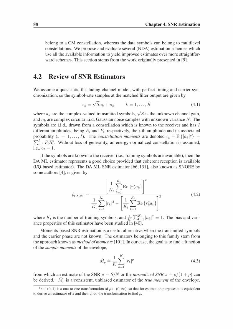
88 Chapter 4. SNR Estimation
belong to a CM constellation, whereas the data symbols can belong to multilevel
constellations. We propose and evaluate several (NDA) estimation schemes which
use all the available information to yield improved estimates over more straightfor-
ward schemes. This section stems from the work originally presented in [9].
4.2 Review of SNR Estimators
We assume a quasistatic flat-fading channel model, with perfect timing and carrier syn-
chronization, so the symbol-rate samples at the matched filter output are given by
rk =√Sak + nk, k = 1, . . . , K (4.1)
where ak are the complex-valued transmitted symbols,√S is the unknown channel gain,
and nk are complex circular i.i.d. Gaussian noise samples with unknown variance N . The
symbols are i.i.d., drawn from a constellation which is known to the receiver and has Idifferent amplitudes, being Ri and Pi, respectively, the i-th amplitude and its associated
probability (i = 1, . . . , I). The constellation moments are denoted cp.= E {|ak|p} =
∑Ii=1 PiR
pi . Without loss of generality, an energy-normalized constellation is assumed,
i.e., c2 = 1.
If the symbols are known to the receiver (i.e., training symbols are available), then the
DA ML estimator represents a good choice provided that coherent reception is available
(I/Q-based estimator). The DA ML SNR estimator [66, 131], also known as SNORE by
some authors [4], is given by
ρDA-ML =
[
1
Kt
Kt∑
k=1
Re {r∗kak}]2
1
Kt
Kt∑
k=1
|rk|2 −[
1
Kt
Kt∑
k=1
Re {r∗kak}]2 (4.2)
where Kt is the number of training symbols, and 1Kt
∑Kt
k=1 |ak|2 = 1. The bias and vari-
ance properties of this estimator have been studied in [40].
Moments-based SNR estimation is a useful alternative when the transmitted symbols
and the carrier phase are not known. The estimators belonging to this family stem from
the approach known as method of moments [101]. In our case, the goal is to find a function
of the sample moments of the envelope,
Mp.=
1
K
K∑
k=1
|rk|p (4.3)
from which an estimate of the SNR ρ.= S/N or the normalized SNR z
.= ρ/(1 + ρ) can
be derived.1 Mp is a consistent, unbiased estimator of the true moment of the envelope,
1z ∈ (0, 1) is a one-to-one transformation of ρ ∈ (0,∞), so that for estimation purposes it is equivalent
to derive an estimator of z and then undo the transformation to find ρ.
4.2. Review of SNR Estimators 89
given by2 [68, 132]
Mp.= E {|rk|p}
= Np
2
I∑
i=1
PiΓ(p
2+ 1)
e−ρR2i1F1
(p
2+ 1; 1; ρR2
i
)
(4.4)
with Γ(·) the gamma function and 1F1(·; ·; ·) the confluent hypergeometric function. For
p even, (4.4) can be seen to admit a simpler form which depends only on the even con-
stellation moments up to order p and the two unknowns ρ, N [86, 110]:
M2n = Nn
n∑
m=0
(n!)2
(n−m)!(m!)2c2mρ
m. (4.5)
Note that (4.5) is a polynomial in ρ, and that in (4.4) and (4.5) the noise power N appears
as a multiplicative factor. This latter fact allows to obtain pure functions of ρ through ratios
of moments in which N vanishes. For example, [68] proposes the family of functions
fk,l(ρ).=
M lk
Mkl
, for k 6= l. (4.6)
An SNR estimate can be then obtained from the sample moments by inversion of fk,l:
ρk,l = f−1k,l
(
M lk
Mkl
)
. (4.7)
In [68] the authors state that fk,l in (4.6) is monotonic.3 This property is a requirement
for any function f(ρ) from whose inverse an estimator is to be derived. The M1M2 and
M2M4 estimators are obtained for (k, l) = (2, 1) and (4, 2) respectively.
4.2.1 Cramer-Rao Bounds for SNR Estimation
The CRB represents the lower variance floor of any unbiased estimator, so it is commonly
used as a benchmark for assessing the competitiveness of the proposed estimators. The
closed form of the CRB for DA I/Q-based estimation was derived in [131] for complex-
valued flat-fading channels, and reads
CRBDA =1
K(2ρ+ ρ2). (4.8)
This CRB, which has been recently shown to be also valid for time-varying channels [167],
is independent of the modulation scheme. In turn, the CRB for the NDA case does de-
pend on the modulation and, unfortunately, does not admit a closed form in general. The
2There is typographical error in Eqs. (3) and (4) of [68]. The complex noise power is defined therein as
N = 2σ2, but the factor 2 does not appear in the expression of the moments.3Although no proof is provided in [68], monotonicity holds for all constellations and all pairs (k, l) we
have tested. Moreover, we have observed that fk,l is monotonically decreasing when k > l, and increasing
when k < l.

90 Chapter 4. SNR Estimation
NDA I/Q-based CRB for BPSK and QPSK was derived in [3], and further discussed
on [166, 167]. NDA I/Q-based CRBs for M -PSK, APSK and 16- and 32-QAM were in-
dependently presented in [69] and [47]. A general form for the NDA I/Q-based CRB for
square QAM modulations has been presented in [19], and subsequently applied to derive
the CRB for SNR estimation in multicarrier systems [20]. Recently, this bound has been
shown to be independent of the knowledge of the carrier phase and frequency [73]
On the other hand, the NDA EVB CRB has been recently presented in [72] for M -
PSK, APSK and 16-QAM modulations. In this section we focus on the EVB setup, so
we will use the NDA EVB CRB as a benchmark when evaluating the performance of the
proposed estimators.
As a rule of thumb, it can be said that the NDA CRB converges to its correspondent
DA CRB for large SNRs, whereas for low SNRs the NDA CRB can be considerably larger
than its DA counterpart. Furthermore, EVB CRBs are at least a factor of 2 larger than the
corresponding I/Q-based CRBs. This last feature follows from the fact that the EVB
approach only considers the magnitude but not the phase, which amounts to discarding
half of the information contained in the samples.
4.3 Higher-Order-Statistics-Based Non-Data-Aided SNR
Estimation
4.3.1 Motivation and Section Outline
The good performance of the sixth-order-based estimator of [110] for two-level constella-
tions suggests that further improvements could be expected if higher-order moments are
allowed in the construction of the estimator. With this in mind, this section investigates
general higher-order approaches for the moments-based SNR estimation problem. The
content of this section is detailed as follows:4
• In Section 4.3.1.1 we identify a novel family of estimators based on ratios of even-
order moments which features an interesting property: all estimators in this family
can be implemented via direct or iterative computations, thus avoiding the need for
lookup tables.
• In Section 4.3.2 we propose a general estimator built upon a linear combination
of members of the previous family, which generalizes the sixth-order approach
of [110] to any (even) order. The weights of the linear combination can be tuned to
each particular constellation and nominal SNR operation range.
• To illustrate the potential of this method, in Section 4.3.3 we develop a statistical
analysis of the particular case in which moments of up to eighth order are allowed,
whereas Section 4.3.4 presents two criteria for weight optimization. These ap-
proaches can be readily generalized to higher-order moments.
4Supporting Mathematica and MATLAB code for some of the algebraic derivations is available online
at [146].

4.3. Higher-Order-Statistics-Based Non-Data-Aided SNR Estimation 91
• As a result, we provide an eighth-order estimator with rather competitive perfor-
mance for non-CM constellations, especially for two- and three-level constellations,
as shown in Section 4.3.5.
• A generalization of the former even-order-based approach to possibly odd-order
moments is proposed in Appendix 4.B, including its statistical analysis.
4.3.1.1 A New Family of NDA Moments-Based Estimators
The analytical inversion of the function fk,l given by (4.6) is intractable in general, as
one may expect from the complexity of (4.4) (an exception is the M2M4 estimate, which
admits a closed-form expression, as we will see below). In such cases one must resort
to precomputed LUTs, as in [23, 68] for the M1M2 estimator. Although LUTs are com-
putationally efficient, their storage requirements, which are proportional to the desired
accuracy, become an issue in hardware implementations with small memory space. This
motivates the search for SNR estimators which do not rely on LUTs.
Consider the following family of functions built upon even-order moments:
f(ρ).=
(U∏
i=1
Mpi2ni
)/
MQ2 , ni, pi ∈ N (4.9)
where Q =∑U
i=1 nipi in order to ensure that the ratio (4.9) does not depend on N . We
refer to 2Q as the statistical order of (4.9). We assume that M2 does not appear in the
numerator (i.e., ni > 1 for all i). Note that (4.9) can be written in terms of the functions
fk,l from (4.7) as f(ρ) =∏U
i=1 fpi/22ni,2
(ρ), so it inherits decreasing monotonicity from the
fk,l family (since 2ni > 2 and pi > 0). In addition, this function exhibits the following
property, whose proof is given in the Appendix:
Property 1. The ratio f(ρ) as defined in (4.9) boils down to a polynomial in z of degree
Q:
f(ρ) =
Q∑
k=0
Fk zk .= F (z). (4.10)
Moreover, the coefficient F1 in (4.10) is always zero.
Now, one can construct SNR estimators by equating F (z) to the sample-moments
version of (4.9), i.e.,
F (z) =
(U∏
i=1
Mpi2ni
)/
MQ2 (4.11)
and then solving for z in (0, 1). Monotonicity of f(ρ) guarantees uniqueness of the so-
lution. This procedure is in fact a polynomial root-finding problem, which may well
be implemented by means of LUTs. Nevertheless, other less memory-costly choices are
possible. On one hand, there exist standard direct algebraic solutions for the roots of poly-
nomials of degree 4 or less (2Q ≤ 8); on the other hand, iterative polynomial root-finding
algorithms can be used, regardless of the order.

92 Chapter 4. SNR Estimation
The popular M2M4 estimator is a particular case of the family (4.9): it is a function of
M4/M22 , which by Property 1 reduces to F (z) = (c4 − 2)z2 + 2. The estimate is hence
given by the positive root of F (z) = M4/M22 :
z =
√
M4/M22 − 2
c4 − 2. (4.12)
The ratio M4/M22 is the lowest-order (2Q = 4) member of this family. The next members,
in growing statistical order, are M6/M32 (2Q = 6), M2
4 /M42 and M8/M
42 (2Q = 8),
M6M4/M52 and M10/M
52 (2Q = 10), and so on.
4.3.2 A New Moments-Based Estimator
The appealing property of ratios of moments of the form (4.9) is that they can be re-
duced to a polynomial in z, so that estimator implementation becomes computationally
simple. This applies as well to any linear combination of these ratios. This fact has been
exploited in [110], where the linear combination f(ρ) = M6/M32 − bM4/M
22 yields a
sixth-order statistics-based estimate with improved behavior for multilevel constellations,
as the weight b can be adjusted depending on the constellation. The good results in terms
of variance attained by this estimator suggest that further improvements could be obtained
by allowing higher-order ratios from the family (4.9) in the linear combination. Two ques-
tions arise at this point. First, how should the ratios featuring in the linear combination be
selected? And second, once these ratios are somehow chosen, how should one select the
weights?
Regarding the first question, there is no straightforward recipe for this “basis selec-
tion” problem. In practice, implementation complexity and finite precision effects would
favor the selection of lower-order moments. On the other hand, including higher-order
terms may be beneficial in terms of estimation bias and/or variance. Therefore, a tradeoff
must be reached balancing these two conflicting goals. As for how to adjust the weights,
it is sensible to optimize them in terms of statistical performance. This issue will be
discussed in Section 4.3.4.
Since the fourth- and sixth-order combinations have been already analyzed in [68]
and [110] respectively, henceforth we focus on the weighted linear combination of all
ratios up to order eight (EOS stands for eighth-order statistics):
fEOS(ρ).= β
M4
M22
+ γM6
M32
+ δM2
4
M42
+ ǫM8
M42
(4.13)
for some weights α = [β γ δ ǫ]T ∈ R4. Note that fEOS(ρ) includes as particular cases
M2M4 (by setting β 6= 0, γ = δ = ǫ = 0) and M6 (β = −b, γ = 1, and δ = ǫ = 0). For
further reference we also define the vector m.= [M2 M4 M6 M8]
T ∈ R4 containing
the true moments appearing in (4.13), and the function hEOS(m).= fEOS(ρ) resulting from
taking m as the independent variable in (4.13).

4.3. Higher-Order-Statistics-Based Non-Data-Aided SNR Estimation 93
After applying the variable change ρ = z/(1− z), one arrives at
FEOS(z) = F4 z4 + F3 z
3 + F2 z2 + F0 (4.14a)
= z2(F4 z2 + F3 z + F2) + F0 (4.14b)
where the coefficients Fk are linear in the weights, and are given by
F4 = δ(c4 − 2)2 + ǫ[72(c4 − 1)− 16c6 + c8] (4.15a)
F3 = (γ + 16ǫ)(12− 9c4 + c6) (4.15b)
F2 = (β + 9γ + 4δ + 72ǫ)(c4 − 2) (4.15c)
F0 = 2(β + 3γ + 2δ + 12ǫ). (4.15d)
The estimator is found by solving for z in
FEOS(z) = βM4
M22
+ γM6
M32
+ δM2
4
M42
+ ǫM8
M42
= hEOS(m) (4.16)
where m.= [M2 M4 M6 M8]
T ∈ R4 is the vector of sample moments. This amounts
to finding the roots of the quartic polynomial FEOS(z) − hEOS(m), in which only the in-
dependent term F0 − hEOS(m) depends on the observations. The roots of quartic poly-
nomials can be algebraically found, although the procedure is somewhat intricate (see
e.g. [1, pp.18-19]). Alternatively, one can resort to root-finding algorithms. For exam-
ple, (4.14b) suggests the following iterative rule:
z(0) = 1, z(n+1) =
√
hEOS(m)− F0
F4(z(n))2 + F3 z(n) + F2
. (4.17)
Note that the polynomial FEOS(z) − hEOS(m) should have a unique root in (0, 1), i.e.,
fEOS(ρ) should be monotonic. Given that the roots depend on the constellation moments
cp as well as on the weights α, one might ask whether conditions on α can be given
ensuring monotonicity of fEOS(ρ); the answer to this question is not trivial. In the next
sections we show how α can be optimized in terms of statistical performance, for a given
constellation and SNR operation range. Let us advance that the optimal weights seem to
yield monotonic functions fEOS(ρ) in the majority of tested cases, with some exceptions
to be discussed in sections 4.3.4 and 4.3.5.
To close this section, let us remark that this EOS approach can be readily general-
ized to higher-order linear combinations of the form similar to (4.13). The presence of
statistics of tenth or greater order will lead to polynomials F (z) of degree 5 or greater.
In such cases, direct computation of the root is not possible, but a root-finding rule of the
form (4.17) always exists, since F1 = 0 by Property 1.
4.3.3 Statistical Analysis
Next we present a small-error analysis to obtain approximate expressions for the variance
and bias of the EOS-based estimate introduced in Section 4.3.2. Our goal is to expose the
dependence of these performance measures with the weight vector α, in order to address
weight optimization in Section 4.3.4. We note that the analytical approach of this section
can be readily generalized to estimators based on higher-order ratios of the form (4.9).

94 Chapter 4. SNR Estimation
4.3.3.1 Variance
From (4.16), the estimator is given by z = F−1EOS
(hEOS(m)).= g(m) and ρ = z/(1− z) =
g(m)/(1 − g(m)).= t(m), where g is implicitly given by FEOS(g) − hEOS(m) = 0.
Following a standard procedure (see e.g. [101, Sec. 9.5]) we consider a first-order Taylor
expansion of the estimator ρ about m = m, which yields the approximation ρ ≈ ρ +vT(m−m), with v
.= ∇t|m=m. Therefore,
Var {ρ} ≈ vTCv (4.18)
with C the covariance matrix of m, whose elements are given by5
[C]ij = (M2(i+j) −M2iM2j)/K, i, j ∈ {1, 2, 3, 4}. (4.19)
The computation of (4.18) is outlined in the Appendix; eventually, one arrives at
Var {ρ} ≈ 1
K
A(Var)(ρ)
B(Var)(ρ)=
1
K
∑10n=0A
(Var)n ρn
∑6n=2B
(Var)n ρn
(4.20)
with A(Var)(ρ).=∑10
n=0A(Var)n ρn and B(Var)(ρ)
.=∑6
n=2B(Var)n ρn. The coefficients of the
former polynomials turn out to be quadratic in α:
A(Var)n = αTA(Var)
n α ⇒ A(Var)(ρ) = αTA(Var)(ρ)α (4.21)
B(Var)n = αTB(Var)
n α ⇒ B(Var)(ρ) = αTB(Var)(ρ)α (4.22)
where the 4 × 4 matrices A(Var)n , B(Var)
n are functions of the constellation moments only,
and A(Var)(ρ) =∑10
n=0A(Var)n ρn, B(Var)(ρ) =
∑6n=2B
(Var)n ρn. Note that (4.20) predicts that
the variance is O(ρ4) at high SNR, similarly to previous results for other estimators based
on ratios of moments [68, 110].
The matrices in (4.21) and (4.22) exhibit interesting properties regardless of the con-
stellation, which we summarize next for further reference. The proofs can be found in the
Appendix.
Property 2. The 4× 4 matrix A(Var)(ρ) has rank not exceeding three.
Property 3. The 4×4 matrix A(Var)10 has rank not exceeding three. In addition, rank
(A
(Var)10
)≤
min{3, I − 1} (recall that I is the number of amplitude levels of the constellation).
Property 4. The 4× 4 matrix B(Var)(ρ) is of the form B(Var)(ρ) = b(Var)(ρ)(b(Var)(ρ))T for
some 4× 1 nonzero vector b(Var)(ρ), and therefore its rank is one.
Property 5. The 4× 4 matrix B(Var)6 is of the form B
(Var)6 = b
(Var)6 (b(Var)
6 )T for some 4× 1nonzero vector b
(Var)6 , and therefore its rank is one.
5Based on the independence of the envelope samples, it is straightforward to show that the variance of
the sample moment Mp (p ∈ N) is given by E {(Mp −Mp)2} = (M2p−M2
p )/K. Similarly, the covariance
of two sample moments Mp, Mq (p, q ∈ N) is seen to be E {(MpMq −MpMq)2} = (Mp+q−MpMq)/K.
4.3. Higher-Order-Statistics-Based Non-Data-Aided SNR Estimation 95
4.3.3.2 Bias
In order to obtain an approximation for the estimation bias, we use a second-order Taylor
expansion of ρ about m = m: ρ ≈ ρ+ vT(m−m) + 12(m−m)TH(m−m), where
H is the Hessian matrix of t(m) evaluated at m = m. Straightforward algebra yields
the approximation
Bias {ρ} ≈ 1
2Tr (HC) . (4.23)
After a few steps, as outlined in the Appendix, one finds
Bias {ρ} ≈ 1
KL(ρ) + J(ρ) Var {ρ} (4.24a)
=1
K
A(L)(ρ)
B(L)(ρ)+
A(J)(ρ)
B(L)(ρ)
1
K
A(Var)(ρ)
B(Var)(ρ)(4.24b)
=1
K
∑12n=0A
(Bias)n ρn
∑9n=3B
(Bias)n ρn
=1
K
A(Bias)(ρ)
B(Bias)(ρ)(4.24c)
where L(ρ).= A(L)(ρ)/B(L)(ρ), with A(L)(ρ) =
∑6n=0A
(L)n ρn, B(L)(ρ) =
∑4n=1B
(L)n ρn,
and J(ρ).= A(J)(ρ)/B(L)(ρ), with A(J)(ρ) =
∑3n=0A
(J)n ρn (note that L(ρ) and J(ρ)
share the same denominator). Furthermore, the former polynomials and their coefficients
are linear in α:
A(L)n = αTa(L)
n ⇒ A(L)(ρ) = αTa(L)(ρ) (4.25)
B(L)n = αTb(L)n ⇒ B(L)(ρ) = αTb(L)(ρ) (4.26)
A(J)n = αTa(J)
n ⇒ A(J)(ρ) = αTa(J)(ρ) (4.27)
where the 4 × 1 vectors a(L)n , b
(L)n , a
(J)n are functions of the constellation moments only,
and a(L)(ρ) =∑6
n=0 a(L)n ρn, b(L)(ρ) =
∑4n=1 b
(L)n ρn, a(J)(ρ) =
∑3n=0 a
(J)n ρn. There-
fore, A(Bias) and B(Bias) are cubic in α. Note that, at high SNR, L(ρ) is O(ρ2) whereas
J(ρ) is O(ρ−1), so (4.24) predicts that the bias is O(ρ3) at high SNR.
4.3.3.3 MSE
Recalling that the minimum square error (MSE) of an estimator is given by MSE {ρ} =Var {ρ}+ Bias2{ρ}, and using (4.20) and (4.24), it is found that
MSE {ρ} ≈ 1
K
∑10n=0A
(Var)n ρn
∑6n=2B
(Var)n ρn
+1
K2
(∑12n=0A
(Bias)n ρn
∑9n=3B
(Bias)n ρn
)2
. (4.28)
Therefore the MSE is the sum of two terms, the first of which (the variance) is O(ρ4)at high SNR and inversely proportional to K, and the second one (the squared bias) is
O(ρ6) at high SNR and inversely proportional to K2. The dependence of the second term
of (4.28) with α is thus of sixth order.

96 Chapter 4. SNR Estimation
4.3.4 Weight Optimization
We focus now on the selection of the weight vector α. Note that the four weights in α
only provide in fact three degrees of freedom, since the solutions to (4.16) are invariant
to scalings in α. This is further emphasized by the fact that the approximations (4.20)
and (4.24) for the variance and the bias are also invariant under this operation. In general,
the number of degrees of freedom in this kind of estimators equals the number of ratios
of moments in the linear combination minus one; for instance, M6 has one degree of free-
dom, whereas M2M4 has none. We present two weight selection procedures, according to
two different optimization criteria. Ideally, one would like to obtain an unbiased estima-
tor with variance close to the theoretical limit dictated by the Cramer-Rao Bound (CRB).
This cannot be achieved with the limited degrees of freedom available, and therefore one
should settle for a less ambitious goal. The question that arises then is how to trade off
bias and variance, and where (i.e., in which SNR operating region).
For example, in [110] the only free parameter in M6 was optimized to yield minimum
variance in the high SNR region. This approach can be generalized to the case in which
several degrees of freedom are available, taking the bias into account as well; we refer
to this criterion as “C1”. Yet other approaches are possible. For instance, systems using
adaptive coding and modulation commonly use each particular constellation within a lim-
ited SNR range (see e.g. [54]). It seems then reasonable to optimize the performance for
some nominal SNR within that range, with the hope that the estimator will still perform
well in a neighborhood of this nominal value. We will refer to this criterion as “C2”. Note
that either C1 or C2 could reasonably be applied to any estimator derived from a linear
combination of the form of (4.13).
4.3.4.1 Criterion C1: Weight Optimization for High SNR
Asymptotically as ρ → ∞, all polynomial divisions A(·)(ρ)/B(·)(ρ) in (4.20) and (4.24)
can be accurately approximated by the first few terms of the quotient polynomial:
Var {ρ} ≈ 1
K
A(Var)(ρ)
B(Var)(ρ).=
1
KC(ρ)
≈ 1
K
(C4 ρ
4 + C3 ρ3 + C2 ρ
2 + C1 ρ+ C0
)(4.29)
L(ρ) ≈ L2 ρ2 + L1 ρ+ L0 (4.30)
J(ρ) ≈ J−1 ρ−1 + J−2 ρ
−2 + J−3 ρ−3. (4.31)
It makes sense now to use the available degrees of freedom to minimize (or, if possible,
cancel) the magnitude of the highest-order coefficients of the variance and the terms of the
bias.6 As for the bias, see (4.24a), it seems convenient to separately minimize L(ρ), J(ρ)
and the variance. In this regard, it must be noted that J−1 = A(J)3 /B
(L)4 = 2 independently
6Alternatively, one could attempt to minimize the highest-order coefficients of the high-SNR approxi-
mation of the MSE. We do not follow this approach, however, in view of the sixth-order dependence with
the weights of some of the terms in (4.28).
4.3. Higher-Order-Statistics-Based Non-Data-Aided SNR Estimation 97
of α and the constellation. This suggests that the minimization efforts should focus on
L(ρ) and the variance. Regarding L(ρ), its highest-order coefficient is given by
L2 =A
(L)6
B(L)4
=αTa
(L)6
αTb(L)4
. (4.32)
Observe that unless a(L)6 and b
(L)4 are collinear (which is not the case with typical con-
stellations), (4.32) can be made zero. Thus, we propose the general principle for weight
optimization in the high SNR region:
Criterion C1: Spend one degree of freedom in α to achieve L2 = 0. Spend the remain-
ing degrees of freedom in order to minimize C4. If C4 can be made zero and there are
degrees of freedom to spare, then proceed to minimize C3, and so on.
With this approach, L(ρ) becomes O(ρ). Note that αTa(L)6 = 0 implies that α = Fα
for some 3×1 vector α, where F is a 4×3 matrix satisfying F TF = I and F Ta(L)6 = 0.
The columns of F can be selected as the three eigenvectors associated to the three nonzero
eigenvalues of the projection matrix
W.= I − a
(L)6 (a
(L)6 )T
||a(L)6 ||2
. (4.33)
Now, the highest-order coefficient of the variance is given by [cf. (4.20)–(4.22) and Prop-
erty 5]
C4 =A(Var)
10
B(Var)6
=αTA
(Var)10 α
αTb(Var)6 (b(Var)
6 )Tα. (4.34)
Thus, for α = Fα, C4 becomes
C4 =αTPα
αTqqTα(4.35)
where P.= F TA
(Var)10 F and q
.= F Tb
(Var)6 . Note that (4.35) is a generalized Rayleigh
quotient with a rank-one denominator matrix. It can be checked that the solution α⋆ to
the minimization of (4.35) (subject to αTq 6= 0) is as follows:
• If P is invertible, then α⋆ = P−1q. The minimized value of C4 is strictly positive.
• If P is singular and rank ([P q]) = rank (P ), then there exist infinitely many
solutions, but all of them yield the same minimized value of C4, which again is
strictly positive. One of these solutions is α⋆ = P+q, where P+ denotes the
pseudoinverse of P .
• If P is singular and rank ([P q]) > rank (P ), then C4 can be made zero. The
solutions can be given in terms of the Singular Value Decomposition (SVD) of P :
P =[U V
][Σ
0
] [UT
V T
]
(4.36)

98 Chapter 4. SNR Estimation
where Σ is positive definite, and U , V have orthonormal columns. Then all the
vectors α⋆ such that Pα⋆ = 0 and αT⋆ q 6= 0 are given (up to a scaling) by
α⋆ = V V Tq + V V T
(
I − qqT
||V Tq||2)
V s (4.37)
where s is arbitrary.
Let r.= rank (A(Var)
10 ), and note that rank (P ) ≤ r. Although in general rank (P ) could
be strictly smaller than r, for all constellations tested it holds that rank (P ) = r. Also,
recall that r ≤ min{3, I − 1} by Property 3. These facts imply that, depending on the
number I of amplitude levels in the constellation, one has the following:
• If I = 1 (CM constellations), then C4 is automatically zero.
• If I = 2, then C4 can be made zero spending just one degree of freedom.
• If I = 3, then C4 can be made zero spending two degrees of freedom.
• If I > 3, then C4 cannot be made zero.
Thus, estimation performance is expected to degrade as the number of levels in the con-
stellation increases. More details are given on each specific case (in terms of I) in Sec-
tion 4.3.5. For reference, Table 4.1 lists the optimal weights α⋆ = F α⋆ under Criterion
C1 for a number of practical multilevel constellations.7
Criterion C1 provides valid estimators for almost all practical constellations, in the
sense that the resulting function fEOS(ρ) in (4.13) is monotonic; the performance obtained
is good in the medium to high SNR range. The only exception we have found is the 16-
QAM constellation, for which the weights provided by Criterion C1 cause the MSE to
exhibit a sharp peak at ρ ≈ 19 dB (the denominators αT⋆ b
(Var)(ρ) and αT⋆ b
(L)(ρ) become
zero for this SNR value). Thus, Criterion C1 is not well suited to 16-QAM.
4.3.4.2 Criterion C2: Weight Optimization for a Nominal SNR Value
Considering a target SNR ρ0 and using Property 4, one can write (4.24) and (4.20) as
Bias {ρ}|ρ=ρ0≈ 1
KL(ρ0) + J(ρ0) Var {ρ}|ρ=ρ0
(4.38)
=1
K
αTa(L)(ρ0)
αTb(L)(ρ0)+
αTa(J)(ρ0)
αTb(L)(ρ0)Var {ρ}|ρ=ρ0
(4.39)
Var {ρ}|ρ=ρ0≈ 1
K
αTA(Var)(ρ0)α
αT b(Var)(ρ0) [b(Var)(ρ0)]T α. (4.40)
Therefore, it is natural to consider the following way of selecting the weights:
Criterion C2: Given a target SNR value ρ0, minimize the approximate variance (4.40)
in terms of α, under the constraint that L(ρ0) in (4.38) be zero.
7The Mathematica and MATLAB code used to derive these optimal weights is available online at [146].

4.3. Higher-Order-Statistics-Based Non-Data-Aided SNR Estimation 99
Table 4.1: Optimal weights (ǫ = 1) under Criterion C1. APSK constellations are as
defined in [54] for the specified code rates
Constellation I β γ δ
16-APSK (2/3) 2 5.9396 −2.8400 −1.4325
16-APSK (3/4) 2 6.0768 −2.8769 −1.4572
16-APSK (4/5) 2 6.1331 −2.8918 −1.4676
16-APSK (5/6) 2 6.1637 −2.8999 −1.4734
16-APSK (8/9) 2 6.2306 −2.9173 −1.4860
16-APSK (9/10) 2 6.2522 −2.9229 −1.4901
32-APSK (3/4) 3 12.3187 −3.8576 −2.7445
32-APSK (4/5) 3 12.0919 −3.8541 −2.7024
32-APSK (5/6) 3 11.9647 −3.8527 −2.6762
32-APSK (8/9) 3 11.6972 −3.8501 −2.6102
32-APSK (9/10) 3 11.6684 −3.8498 −2.6027
16-QAM 3 9.9411 −5.28 −0.2807
32-QAM 5 10.2400 −3.8552 −2.1227
64-QAM 9 10.7991 −4.3509 −1.8525
128-QAM 16 10.7081 −4.1297 −2.0170
256-QAM 32 10.4846 −4.4251 −1.6505
This criterion amounts to minimizing a generalized Rayleigh quotient with a rank-one
denominator matrix, subject to a linear constraint. This is analogous to the case encoun-
tered for Criterion C1. The only difference is that now the objective function (4.40) cannot
be made zero, as it corresponds to the estimator variance (and not just one coefficient in
its Taylor series expansion). Therefore, the solution is given (up to a scaling) by
α⋆(ρ0) = F(F TA(Var)(ρ0)F
)−1F Tb(Var)(ρ0) (4.41)
where the columns of the 4×3 matrix F are now given by the three eigenvectors associated
to the three nonzero eigenvalues of
W = I − a(L)(ρ0)[a(L)(ρ0)]
T
||a(L)(ρ0)||2. (4.42)
This SNR-dependent solution α⋆(ρ0) proves in most cases competitive within a few
dBs about ρ0. Nevertheless, one must evaluate its performance in the entire SNR range for
each particular constellation and target SNR, as α⋆(ρ0) could yield an invalid estimator
in some SNR interval (i.e. fEOS(ρ) in (4.13) could turn out to be non-monotonic). Of all
constellations tested, only the 16-APSK family suffers from this problem, but only within
some limited SNR intervals, as shown in the next section.
Note that in (4.38)-(4.39) the factor J(ρ0) has the same form as L(ρ0), and therefore,
in contrast to Criterion C1, it could be made zero using one degree of freedom in α.

100 Chapter 4. SNR Estimation
This suggests an alternative criterion, in which one of the degrees of freedom used for
minimizing the variance under Criterion C2 would be used instead for canceling J(ρ0)(and therefore completely canceling the bias at ρ0). However, the solutions provided by
this alternative criterion turn out to be problematic in practice (fEOS(ρ) is not monotonic
for most constellations; sharp peaks appear in bias and variance at certain SNRs), and
hence it will not be further considered here.
4.3.5 Performance Results
The performance of the proposed estimators strongly depends on the number of levels of
the constellation. Next we discuss the results achieved with criteria C1 and C2 with
respect to existing estimates of the same kind: M2M4 and M6. We show results for
the dependence of the bias with the SNR, and the dependence of the SNR-normalized
MSE with the SNR and the sample size K. The SNR-normalized MSE is defined as
NMSE {ρ} .= MSE {ρ} /ρ2. The NDA-EVB CRB (numerically evaluated as in [72]) is
provided as benchmark. Analytical results are completed with empirical results obtained
through simulations, in which each point was averaged over 10 000 realizations.
4.3.5.1 CM constellations
CM constellations (for which cp = 1, for all p) constitute a special case, as it turns out
that A(L)6 = 0 whereas A
(L)5 6= 0 (with B
(L)4 6= 0), and that A(Var)
10 = A(Var)9 = 0 whereas
A(Var)8 6= 0 (with B(Var)
6 6= 0). Therefore, the bias and variance are respectively linear and
quadratic in ρ for general α. Interestingly, the highest-order coefficients of L(ρ) and of the
variance turn out to be independent of α: A(L)5 /B
(L)4 = 1 and A(Var)
8 /B(Var)6 = 2. It makes
sense then to use a modified version of Criterion C1, focusing for example on the lowest-
order coefficient of the variance A(Var)0 /B(Var)
2 , which dominates in the region of low SNR.
This term is minimized for α⋆ = [β 0 δ 0]T, where β and δ cannot be both zero;
the attained variance is Var {ρ} ≈ (2ρ4 + 8ρ3 + 10ρ2 + 6ρ + 1)/(Kρ2), independently
of β and δ, and coincides with that of the M2M4 estimator for CM constellations [68].
The predicted MSE turns out to remain quite close to the CRB throughout the entire SNR
range.
4.3.5.2 Two-level Constellations
When I = 2, application of Criterion C1 with the available degrees of freedom results
in L2 = C4 = C3 = 0. In this case, it is possible to obtain closed-form expressions for
the optimal weights in terms of the probabilities p = P1, 1 − p = P2, and the ring ratio

4.3. Higher-Order-Statistics-Based Non-Data-Aided SNR Estimation 101
w = R2/R1:
β =(1 + w2) [3w6 + w4 + 3p2(1 + w2)(1 + w4)− 2p(3w6 + 2w4 + w2)]
[p2 − (1− p)2w4]2· ǫ
γ = − 2(1 + w2)
p+ (1− p)w2· ǫ
δ = − p+ (1− p)w4
[p− (1− p)w2]2· ǫ, ǫ 6= 0.
As a result, Criterion C1 achieves O(ρ2) in the variance and the MSE, which is the lowest
possible order as dictated by the CRB [72]. In contrast, the variances of M6 and M2M4
are respectively O(ρ3) and O(ρ4), and their respective MSEs are O(ρ4) and O(ρ6).
Figures 4.1a and 4.1b show the bias and the NMSE vs. the SNR (for K = 1000samples) for one of the 16-APSK constellations specified in [54] (P1 = 1/4, P2 = 3/4,
R2/R1 = 3.15). The bias under Criterion C1 remains small, and the improvement in
NMSE at high SNR is evident. Still, the gap to the CRB is not negligible. Note that for
ρ < 22 dB, M6 achieves a slightly lower NMSE than Criterion C1, but its performance
quickly degrades beyond this point.
Results for Criterion C2 with ρ0 = 20 dB are also displayed in Figure 4.1b, showing
that this is in fact a good strategy in the vicinity of ρ0 (it outperforms the rest of estimators
between 15 and 22 dB), but also for ρ < ρ0, where its NMSE is never larger than that
provided by Criterion C1 (this seems to hold regardless of the value of ρ0). From a
designer’s perspective, setting the target SNR ρ0 near the upper limit of the SNR operation
range seems an appropriate choice.
For reference, Figure 4.1b also shows the “genie-aided” NMSE curve, obtained by
choosing the optimal α⋆(ρ) under Criterion C2 for each ρ. This gives a lower bound on
the NMSE for the proposed eighth-order estimator. Note that the genie-aided curve ap-
proaches the CRB as the SNR increases. Hence, within this region, the estimator designed
under Criterion C2 is near optimal at the target SNR. In the low SNR region (below 5 dB),
M2M4 attains the genie-aided curve; however, neither M2M4, nor M6, nor Criterion C1
can reach genie-aided performance above 5 dB. In general, good agreement is observed
between theory and simulations.
As mentioned in Section 4.3.4.2, Criterion C2 may yield invalid estimators for certain
values of ρ0. For the 16-APSK constellation of Figure 4.1b, this happens for ρ0 between 5
and 15 dB. In this case one could fall back on some suboptimal solution, e.g., use the valid
C2 estimator for ρ0 = 15 dB, which offers good performance (not shown in Figure 4.1)
in this SNR interval.
Figure 4.1c shows the variation of the NMSE with the number of observed samples
K, for SNR = 20 dB. It is seen that, for all estimators, the empirical results agree with
the predicted theoretical values as long as the corresponding NMSE is sufficiently small
(which is an indicator of the accuracy of the Taylor series approximation used to obtain
the theoretical expressions). Note that the new EOS estimators outperform the M2M4 and
M6 schemes in the sense that they can achieve the same NMSE with significantly fewer
samples. This holds true also for other SNR values.
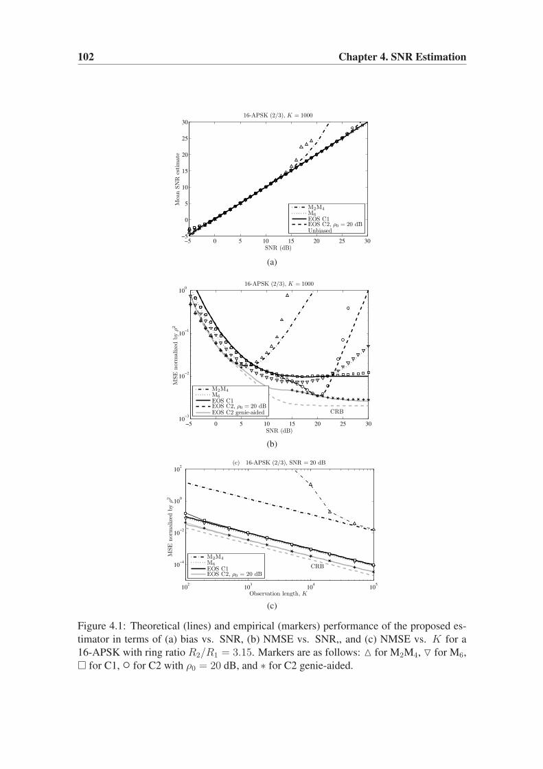
102 Chapter 4. SNR Estimation
−5 0 5 10 15 20 25 30−5
0
5
10
15
20
25
30
SNR (dB)
Mea
nSN
Res
tim
ate
16-APSK (2/3), K = 1000
M2M4M6EOS C1EOS C2, ρ0 = 20 dBUnbiased
(a)
−5 0 5 10 15 20 25 3010
−3
10−2
10−1
100
SNR (dB)
MSE
nor
mal
ized
by
ρ2
16-APSK (2/3), K = 1000
CRB
M2M4M6EOS C1EOS C2, ρ0 = 20 dBEOS C2 genie-aided
(b)
102
103
104
105
10−4
10−2
100
102
Observation length, K
MSE
nor
mal
ized
by
ρ2
(c) 16-APSK (2/3), SNR = 20 dB
CRB
M2M4M6EOS C1EOS C2, ρ0 = 20 dB
(c)
Figure 4.1: Theoretical (lines) and empirical (markers) performance of the proposed es-
timator in terms of (a) bias vs. SNR, (b) NMSE vs. SNR,, and (c) NMSE vs. K for a
16-APSK with ring ratio R2/R1 = 3.15. Markers are as follows: △ for M2M4, ▽ for M6,
� for C1, ◦ for C2 with ρ0 = 20 dB, and ∗ for C2 genie-aided.

4.3. Higher-Order-Statistics-Based Non-Data-Aided SNR Estimation 103
4.3.5.3 Three-level Constellations
For I = 3, application of Criterion C1 with the available degrees of freedom results
in L2 = C4 = 0. The resulting variance and MSE are respectively O(ρ3) and O(ρ4),a remarkable improvement over M2M4 and M6, which are both O(ρ4) (variance) and
O(ρ6) (MSE). This can be seen in Figures 4.2a and 4.2b, which display the bias, and
the NMSE vs. the SNR (for K = 1000 samples) for one of the 32-APSK constellation
specified in [54] (P1 = 1/4, P2 = 3/8, P3 = 1/2, R2/R1 = 2.84, R3/R1 = 5.27).
Good agreement is observed between theory and simulations. M6 and Criterion C2 with
ρ0 = 20 dB remain close to the genie-aided case between 5 and 10 dB, and between 12
and 21 dB, respectively. Note that the genie-aided curve does not approach the CRB in
this case. Figure 4.3c displays the dependence of the NMSE with K (for SNR = 20 dB).
As observed for 16-APSK, the theoretical analysis proves useful for sufficiently small
NMSE, and the EOS estimators outperform M2M4 and M6 in terms of K.
As mentioned in Section 4.3.4.1, Criterion C1 fails to provide a good estimator for
the 16-QAM constellation, see Figure 4.3. The estimator designed under Criterion C1 is
severely biased above 14 dB, and below that SNR its NMSE is outperformed by those
of M2M4 and M6 (observe also the peak in the theoretical NMSE at about 19 dB). From
Figures 4.3b and 4.3c it is seen that M6 almost achieves genie-aided performance above
10 dB, which suggests that the EOS approach is not advantageous for 16-QAM. Compar-
ison with Figure 4.2 shows that the best NMSEs obtained at intermediate-to-high SNR
for 16-QAM are substantially higher than those obtained for 32-APSK, for all moments-
based methods. Thus, the arrangement of signal points for 16-QAM seems to be particu-
larly challenging to this class of estimators.
4.3.5.4 Constellations with More than Three Levels
For I ≥ 4, application of Criterion C1 with the available degrees of freedom results in
L2 = 0 and C4 > 0. The resulting variance and MSE are therefore O(ρ4) and O(ρ6),respectively. Nevertheless, this approach is still useful, as shown in Figure 4.4, which
shows the results obtained with 32-QAM (I = 5). In terms of NMSE, (Figure 4.4b,
K = 1000 samples), Criterion C1 clearly improves over M2M4 and M6 in the high SNR
region. M2M4 achieves close-to-genie-aided performance below 6 dB, whereas M6 takes
over between 7 and 13 dB. For higher SNR, criteria C1 and C2 (ρ0 = 20 dB), which
show almost identical performance, are the most competitive. The results in terms of K(Figure 4.4c) confirm the same trend observed for 16-APSK and 32-APSK.
The behavior for other QAM constellations with more than three levels is similar to
that of Figure 4.4. We must note that the performance improvement obtained with eighth-
order estimators at high SNR is observed to be greater for cross-QAM constellations (32-,
128-QAM) than for square QAMs (64-, 256-QAM).
Summarizing, we have seen that the use of higher-order moments is an interesting
approach for estimator design. The proposed eighth-order SNR estimator features three
degrees of freedom which have been used to optimize the performance of the estimator
according to two different criteria. Both criteria have proven useful to yield an improved
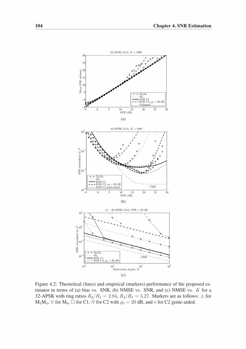
104 Chapter 4. SNR Estimation
−5 0 5 10 15 20 25 30−5
0
5
10
15
20
25
30
SNR (dB)
Mea
nSN
Res
tim
ate
32-APSK (3/4), K = 1000
M2M4M6EOS C1EOS C2, ρ0 = 20 dBUnbiased
(a)
−5 0 5 10 15 20 25 3010
−3
10−2
10−1
100
SNR (dB)
MSE
nor
mal
ized
by
ρ2
32-APSK (3/4), K = 1000
CRB
M2M4M6EOS C1EOS C2, ρ0 = 20 dBEOS C2 genie-aided
(b)
102
103
104
105
10−4
10−2
100
102
Observation length, K
MSE
nor
mal
ized
by
ρ2
(c) 32-APSK (3/4), SNR = 20 dB
CRB
M2M4M6EOS C1EOS C2, ρ0 = 20 dB
(c)
Figure 4.2: Theoretical (lines) and empirical (markers) performance of the proposed es-
timator in terms of (a) bias vs. SNR, (b) NMSE vs. SNR, and (c) NMSE vs. K for a
32-APSK with ring ratios R2/R1 = 2.84, R3/R1 = 5.27. Markers are as follows: △ for
M2M4, ▽ for M6, � for C1, ◦ for C2 with ρ0 = 20 dB, and ∗ for C2 genie-aided.

4.3. Higher-Order-Statistics-Based Non-Data-Aided SNR Estimation 105
−5 0 5 10 15 20 25 30−5
0
5
10
15
20
25
30
SNR (dB)
Mea
nSN
Res
tim
ate
16-QAM, K = 1000
M2M4M6EOS C1EOS C2, ρ0 = 20 dBUnbiased
(a)
−5 0 5 10 15 20 25 3010
−3
10−2
10−1
100
101
102
SNR (dB)
MSE
nor
mal
ized
by
ρ2
16-QAM, K = 1000
CRB
M2M4
M6
EOS C1EOS C2, ρ0 = 20 dBEOS C2 genie-aided
(b)
102
103
104
105
10−4
10−2
100
102
Observation length, K
MSE
nor
mal
ized
by
ρ2
16-QAM, SNR = 15 dB
CRB
M2M4
M6
EOS C1
EOS C2, ρ0 = 15 dB
(c)
Figure 4.3: Theoretical (lines) and empirical (markers) performance of the proposed es-
timator in terms of (a) bias vs. SNR, (b) NMSE vs. SNR, and (c) NMSE vs. K for
16-QAM. Markers are as follows: △ for M2M4, ▽ for M6, � for C1, ◦ for C2 with
ρ0 = 20 dB, and ∗ for C2 genie-aided.
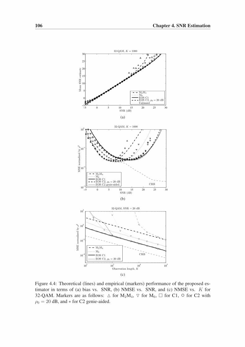
106 Chapter 4. SNR Estimation
−5 0 5 10 15 20 25 30−5
0
5
10
15
20
25
30
SNR (dB)
Mea
nSN
Res
tim
ate
32-QAM, K = 1000
M2M4M6EOS C1EOS C2, ρ0 = 20 dBUnbiased
(a)
−5 0 5 10 15 20 25 3010
−3
10−2
10−1
100
SNR (dB)
MSE
nor
mal
ized
by
ρ2
32-QAM, K = 1000
CRB
M2M4M6EOS C1EOS C2, ρ0 = 20 dBEOS C2 genie-aided
(b)
102
103
104
105
10−4
10−2
100
102
Observation length, K
MSE
nor
malize
dby
ρ2
32-QAM, SNR = 20 dB
CRB
M2M4
M6
EOS C1
EOS C2, ρ0 = 20 dB
(c)
Figure 4.4: Theoretical (lines) and empirical (markers) performance of the proposed es-
timator in terms of (a) bias vs. SNR, (b) NMSE vs. SNR, and (c) NMSE vs. K for
32-QAM. Markers are as follows: △ for M2M4, ▽ for M6, � for C1, ◦ for C2 with
ρ0 = 20 dB, and ∗ for C2 genie-aided.

4.4. SNR Estimation with Heterogeneous Frames 107
performance over previous moments-based estimators. The improvement is remarkable
in the case of two-level constellations and most of three-level constellations.
4.4 SNR Estimation with Heterogeneous Frames
4.4.1 Introduction
Whereas most NDA SNR estimators exploit the knowledge of the underlying constel-
lation, in certain situations the observed frame consists of several subframes, with the
particular feature that the symbols in different subframes are drawn from different con-
stellations. We shall refer to this kind of frames as heterogeneous, as opposed to homo-
geneous frames composed of symbols from one single constellation. For example, the
DVB-S2 standard [54] allows frames in which the data symbols belong either to QPSK,
8-PSK, 16-APSK or 32-APSK. In all of those cases, the frame header and, optionally,
some extra pilot symbols within the frame can be assumed to be drawn from a QPSK
constellation. Since available NDA SNR estimators are tailored to a given constellation,
it is not immediate how to generalize their use to these heterogeneous frame scenarios.
Each constituent subframe contains a different quantity of information depending on its
number of symbols and the constellation used. One obvious approach is to use only one
of the subframes, but this results in inefficient use of the available data. This motivates
the search for techniques making use of the whole observation set, in order to improve
estimation performance. In our study we will consider both NDA EVB SNR estimators
and DA estimators.
In this section we analyze the estimation problem with heterogeneous frames. We
derive the CRB for the problem and we propose a number of estimators (Section 4.4.3).
Then we evaluate the proposed solutions in some practical scenarios (Section 4.4.4). The
evaluation is performed both analytically and empirically through Monte Carlo simula-
tions.
4.4.2 Signal Model for a Heterogeneous Frame
We assume the same flat-fading signal model given in (4.1), with the exception that the
original symbols belong to different constellations. Hence, the baud rate sampled output
of the matched filter is given by
rk =√Sak + nk, k ∈ {1, . . . , K} = K1 ∪ K2 (4.43)
where ak are statistically independent complex valued transmitted symbols,√S is the un-
known channel gain, and nk are independent zero-mean circular Gaussian noise samples
with unknown variance N . The transmitted symbol sequence {ak, k ∈ K1 ∪ K2} con-
forms a heterogeneous frame. The disjoint sets K1, K2 (known by the receiver) contain
the indices of, respectively, the K1 and K2 symbols (K1 + K2 = K) drawn from con-
stellations A1 and A2, which have respectively I1 and I2 amplitude levels (e.g. I1 = 1 if

108 Chapter 4. SNR Estimation
Figure 4.5: Example of a heterogeneous frame containing symbols from two different
constellations A1, A2.
A1 is M -PSK and I2 = 3 if A2 is 32-APSK). The n-th order moment of Ai is denoted as
c(i)n
.= E {|ak|n}, where k ∈ Ki. In this section we will use the superindex (i) to denote
that the estimation is performed over the symbols corresponding to constellation Ai. It
will be useful for us to define the ratio p.= K1/(K1 + K2). An example of a heteroge-
neous frame containing symbols from two different constellations is shown in Figure 4.5.
For reference throughout this section we have selected two practical cases of applica-
tion with different heterogeneous frames which are based on the framing structure pro-
vided by the DVB-S2 standard [54]. This standard admits two frame lengths: short frames
(carrying 16200 data bits) and normal frames (carrying 64800 bits). The inclusion of pi-
lots is optional. The structure of a DVB-S2 frame is shown in Figure 4.6, and can be
broken down as follows:
• Header. The header is composed of 90 π/2 BPSK symbols.8 The first 26 sym-
bols constitute the SOF (Start of Frame), and have a fixed value. The remaining 64
symbols constitute the so-called PLSCODE (Physical Layer Signaling code) which
indicates the frame length, the possible use of pilots, and the MODCOD (modula-
tion and coding rate) used in the data blocks.
• Data bearing blocks. Data symbols are placed in slots of 90 symbols. The total
number of slots depends on the frame length and the code rate. The following
modulations are allowed for the data symbols: QPSK, 8PSK, 16-APSK and 32-
APSK. A number of code rates are valid for each modulation.
• Pilot blocks. When pilots are used, one block of 36 pilot symbols is inserted each
16 data slots. Again, the total number of pilot symbols depends on the frame length
and code rate. All pilot symbols take the value (1 + j)/√2. Note that such value
corresponds to the first quadrant symbol of a QPSK constellation normalized in
energy.
The two heterogeneous frames considered for evaluation, namely HF1 and HF2, are de-
scribed as follows:
HF1) This frame is a DVB-S2 short frame in which A1 = QPSK, K1 = 162, A2 = 32-
APSK (code rate 3/4), K2 = 3240 (therefore p ≈ 0.0475), with Kt = 98 known
training symbols. In the K1 QPSK symbols we include not only the pilots inserted
8The π/2 BPSK modulation is composed of complex-valued symbols carrying only one information
bit. Assuming energy normalization, odd symbols take values in {(1 + j)/√2, (−1 − j)/
√2}, whereas
even symbols take values in {(1 − j)/√2, (−1 + j)/
√2}. Hence, disregarding this alternating structure,
π/2 BPSK symbols can be perfectly considered as QPSK symbols.

4.4. SNR Estimation with Heterogeneous Frames 109
Figure 4.6: Structure of a DVB-S2 frame.
within the frame, but also the π/2 BPSK symbols of the frame header, which for
SNR estimation purposes can be regarded as QPSK.
HF2) This is not a DVB-S2 compliant frame containing pilots with A1 = QPSK, K1 =162, A2 = 16-APSK (equivalent to that used in the DVB-S2 standard for code rate
3/4), K2 = 1458 (therefore p = 0.1), Kt = 98.
The reason why Kt 6= K1 in the frames described above is the following. Consider
the case HF1, where K1 contains the indices of the QPSK symbols. According to the
DVB-S2 standard, a short 32-APSK frame using pilots has 90 header symbols and 72
pilots. From the 90 symbols in the header, however, only those 26 conforming the SOF
are known to the receiver, and thus the difference of 64 symbols between Kt and K1. This
has been assumed for case HF2 too. The existence of training symbols allows the use of
DA SNR estimation schemes. This has been taken into account in the results reported in
Section 4.4.4.
4.4.3 Proposed SNR Estimators
With heterogeneous frames, the choice of an SNR estimator is not straightforward. If
one is to apply an available estimator for each subframe and then select the one with
lower MSE, the final choice would depend on the true SNR, the constellations, and the
sample sizes. For example, suppose K1 = 1, K2 > 1, and K2 ≫ K1. This last fact could
suggest that a single estimator over the subset K2 be employed. However, the performance
of standard NDA SNR estimators severely degrades with multilevel constellations, as we
have seen in Section 4.3, and hence using the data from subset K1 may result in significant
improvement even if the corresponding number of samples is relatively small.
Another possibility is to use a single estimator for the whole set, upon defining the
aggregate constellation A0 = A1 ∪ A2 with new moments c(0)p . This approach, however,
does not exploit knowledge of the index sets Ki; moreover, since the I1 levels of A1
and the I2 levels of A2 need not coincide, A0 will present a larger number of levels
I0 = I1 + I2, which can be expected to further degrade estimator performance. This
motivates alternative techniques exploiting all available data. In the rest of this section
we first provide the procedure to obtain the CRB for this problem, and then we present
a number of SNR estimators which make use of the whole set of received samples. For

110 Chapter 4. SNR Estimation
further reference, ρ24 will be used to denote the M2M4 estimator, and ρ6 will denote the
sixth-order estimator of [110].
4.4.3.1 Cramer-Rao Lower Bound
Let φ = [ρ,N ] be the vector of unknown parameters. Since the observations are statisti-
cally independent, the Fisher information matrix (FIM) satisfies F (φ) = F1(φ)+F2(φ),where Fi(φ) is the FIM for the estimation problem using only {rk, k ∈ Ki}. Now
Fi(φ) = KiFi(φ), where Fi(φ) does not depend on Ki. Hence,
F−1(φ) =1
K
[pF1(φ) + (1− p)F2(φ)
]−1(4.44)
and Var {ρ} ≥ [F−1(φ)]11 for any unbiased estimate ρ. Depending on the information
available, the FIM should be computed differently. In the coherent DA case, one has
Ft(φ) = Kt
1
2ρ
1
2N
1
2N
2 + ρ
2N2
. (4.45)
For the NDA EVB case, the FIM must be computed numerically; see e.g. [72].
4.4.3.2 Expectation-Maximization (EM) Estimator
In principle, one could attempt to maximize the Log-likelihood Function (LLF) of the
parameters, which is the sum of the individual LLFs over each subframe. This Maxi-
mum Likelihood (ML) approach requires numerical optimization and is computationally
expensive. As a cheaper alternative, the EM algorithm can be applied. In [72], the EM
algorithm for homogeneous frames was derived in the EVB NDA setting. This approach
can be readily modified to fit heterogeneous frames, as it allows to incorporate informa-
tion about the underlying constellation for each individual symbol in the frame. The fact
that the conditional pdf is not Gaussian (since only the envelope is considered) makes nec-
essary to use suitable high-SNR approximations, so that the performance of the EM SNR
estimator degrades as the SNR decreases [111]. In particular, a non-negligible bias shows
up when applied to cases HF1, HF2, and therefore we do not include its performance in
this work.
4.4.3.3 Convex Combination of Estimates (CCE)
Suppose that two unbiased estimators ρ(i) obtained from samples in subframes i = 1, 2,
are available. Then the convex combination
ρcce = λcce · ρ(1) + (1− λcce) · ρ(2) (4.46)

4.4. SNR Estimation with Heterogeneous Frames 111
−5 0 5 10 15 20 25 30
0.2
0.4
0.6
0.8
1
SNR (dB)
λ∗ cc
e
C1
12.5 13 13.50.3
0.35
0.4
SNR (dB)
ρ(1)24 , ρ
(2)6
ρ(1)da-ml
, ρ(2)6
Figure 4.7: λ⋆cce as a function of the SNR for CCE: case HF1, with {ρ(1)24 , ρ
(2)6 } and {ρ(1)DA-ML,
ρ(2)6 }. The inset zooms in the region of operation of the DVB-S2 32-APSK 3/4 MOD-
COD. The trade-off values for λcce, marked as circles, are taken from the center of the
working SNR interval (delimited by vertical dotted lines).
is also an unbiased estimator. Its variance is readily found to be
σ2cce = λ2
cceσ21 + (1− λcce)
2σ22 (4.47)
where σ2i.= Var
{ρ(i)}
. This variance has a minimum value
σ2cce,⋆ =
σ21 σ
22
σ21 + σ2
2
which is achieved by the optimal choice
λ⋆cce =
σ22
σ21 + σ2
2
. (4.48)
This approach is motivated by the following fact: suppose that φ(i) were efficient esti-
mates restricted to each subframe i = 1, 2 [i.e. their covariance matrices are F−1i (φ)].
Then φ = Wφ(1) + (I −W )φ(2) is an efficient estimate (considering all the frame), i.e.
its covariance matrix is given by (4.44). The weight W depends in general on the true
parameter and is given by W = F−12 (φ)
[F−1
1 (φ) + F−12 (φ)
]−1. Thus, convex combi-
nations of estimates are attractive, although in practice the constituent estimators need not
be efficient.
In order to choose λcce, the true variances σ21 , σ2
2 are needed. Since in general they
depend on ρ, a trade-off must be reached in order to obtain acceptable performance over
the whole operation range. To illustrate this, let us consider case HF1, and assume an
NDA-NDA CCE with {ρ(1)24 , ρ(2)6 }, and a DA-NDA CCE with {ρ(1)DA-ML, ρ
(2)6 } are used

112 Chapter 4. SNR Estimation
−5 0 5 10 15 20 25 30
10−2
10−1
100
SNR (dB)
Norm
alize
dV
ariance
C1
ρ(1)24
ρ(2)6ρ
(1)DA−ML
Constituent estimator
CCE 24(1)−−6(2)
CCE DA−ML(1)−−6(2)
CCE 24(1)−−6(2) with λtrade−off
= 0.3339
CCE DA−ML(1)−−6(2) with λtrade−off
= 0.3865
Figure 4.8: Case HF1: Analytical variances of ρ(1)24 , ρ
(1)DA-ML, ρ
(2)6 and the combined es-
timators ρcce for the optimal SNR dependent values λ⋆cce and for the trade-off values
λtrade-offcce,24−6 = 0.3339, λtrade-off
cce,DA-ML−6 = 0.3865.
in the corresponding subframes.9 Since analytical approximate expressions are known
for the variances of ρ(1)24 , ρ
(1)DA-ML and ρ
(2)6 [40, 68, 110], it is possible to plot λ⋆
cce in terms
of ρ, as in Figure 4.7. According to the DVB-S2 standard, the MODCOD 32-APSK
3/4 is expected to be used in the SNR range [12.73 dB, 13.64 dB], shown in the inset
of Figure 4.7, and where tentative trade-off values for λcce are marked. These values
λtrade-offcce,24−6 = 0.3339, λtrade-off
cce,DA-ML−6 = 0.3865 have been chosen as the value of λ⋆cce at the
center of the nominal SNR working range of the selected DVB-S2 MODCOD.
Figure 4.8 shows the analytical variance of ρcce using the optimal value λ⋆cce(ρ), marked
with thicker lines, and the analytical variance obtained with λtrade-offcce . The variances of
the two constituent estimators are shown for comparison. It can be seen that the CCE
estimators consistently outperform the better of the two constituent estimators over a wide
SNR range. In general, the largest improvement is achieved when the variances of the
original estimators are equal; in this case λ⋆cce = 0.5 and the CCE method yields a 3 dB
reduction in estimation variance. This can be observed around SNR ≈ 15 − 16 dB in
Figure 4.8. Also, it can be seen that the selected λtrade-offcce perform very close to the optimal
value not only in the desired SNR range, but also outside of it.
We remark that the CCE approach is not limited to constituent moment-based estima-
tors. Any two independent unbiased estimators can be used, as long as their true variances
are known or can be analytically or empirically approximated, in order to select λcce.
9We note that in the DA-NDA approach, only Kt of the K1 symbols of subframe 1 are being used by the
DA-ML estimator; thus there are K1 −Kt = 64 symbols that remain unused. In this case, one could define
a third subframe with those 64 QPSK symbols to which an NDA estimator should be applied, yielding
an overall DA-NDA-NDA estimator over three subframes. The CCE approach can be straightforwardly
extended to more than two subframes, although we restrict our analysis to two subframes for the sake of
simplicity.
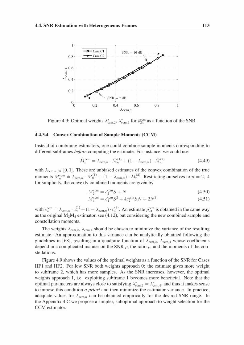
4.4. SNR Estimation with Heterogeneous Frames 113
0 0.2 0.4 0.6 0.8 10
0.2
0.4
0.6
0.8
1
λccm,2
λcc
m,4
Case C1
Case C2
SNR = 7 dB
SNR = 16 dB
Figure 4.9: Optimal weights λ∗ccm,2, λ
∗ccm,4 for ρccm
24 as a function of the SNR.
4.4.3.4 Convex Combination of Sample Moments (CCM)
Instead of combining estimators, one could combine sample moments corresponding to
different subframes before computing the estimate. For instance, we could use
M ccmn = λccm,n · M (1)
n + (1− λccm,n) · M (2)n (4.49)
with λccm,n ∈ [0, 1]. These are unbiased estimates of the convex combination of the true
moments M ccmn
.= λccm,n ·M (1)
n + (1 − λccm,n) ·M (2)n . Restricting ourselves to n = 2, 4
for simplicity, the convexly combined moments are given by
M ccm2 = cccm
2 S +N (4.50)
M ccm4 = cccm
4 S2 + 4cccm2 SN + 2N2 (4.51)
with cccmn
.= λccm,n · c(1)n + (1− λccm,n) · c(2)n . An estimate ρccm
24 is obtained in the same way
as the original M2M4 estimator, see (4.12), but considering the new combined sample and
constellation moments.
The weights λccm,2, λccm,4 should be chosen to minimize the variance of the resulting
estimate. An approximation to this variance can be analytically obtained following the
guidelines in [68], resulting in a quadratic function of λccm,2, λccm,4 whose coefficients
depend in a complicated manner on the SNR ρ, the ratio p, and the moments of the con-
stellations.
Figure 4.9 shows the values of the optimal weights as a function of the SNR for Cases
HF1 and HF2. For low SNR both weights approach 0: the estimate gives more weight
to subframe 2, which has more samples. As the SNR increases, however, the optimal
weights approach 1, i.e. exploiting subframe 1 becomes more beneficial. Note that the
optimal parameters are always close to satisfying λ∗ccm,2 = λ∗
ccm,4, and thus it makes sense
to impose this condition a priori and then minimize the estimator variance. In practice,
adequate values for λccm,n can be obtained empirically for the desired SNR range. In
the Appendix 4.C we propose a simpler, suboptimal approach to weight selection for the
CCM estimator.

114 Chapter 4. SNR Estimation
4.4.3.5 Weighted Least Squares (WLS) Approach
Using (4.5) we can obtain estimates of S and N by matching the theoretical and sample
second and fourth order moments for the two subframes: for i = 1, 2,
M(i)2 = c
(i)2 S + N , (4.52a)
M(i)4 = c
(i)4 S2 + 4c
(i)2 SN + 2N2. (4.52b)
These four equations in two unknowns suggest a weighted LS approach to estimate S and
N .10 However, this is a nonlinear problem with no straightforward closed-form solution.
However, if we take N = M(i)2 − c
(i)2 S in (4.52a) and substitute this back in (4.52b), we
obtain two linear equations in S2:
[
c(i)4 − 2
(c(i)2
)2]
S2 = M(i)4 − 2
(M
(i)2
)2, i = 1, 2. (4.53)
Let wi, i = 1, 2 be the weights associated to each subframe, with w2 = 1− w1. Then the
WLS solution to (4.53) is
SWLS =
√
w1γ1δ1 + w2γ2δ2w1γ2
1 + w2γ22
(4.54)
with δi = M(i)4 − 2
(M
(i)2
)2and γi = c
(i)4 − 2
(c(i)2
)2. With this value, we now obtain the
WLS solution to M(i)2 = c
(i)2 SWLS + N , i = 1, 2, which is
NWLS = [w1M(1)2 + w2M
(2)2 ]− [w1c
(1)2 + w2c
(2)2 ]SWLS. (4.55)
Note that w1 = 1 yields ρ(1)24 , and w1 = 0 yields ρ
(2)24 . The weights wi should be chosen
to yield minimum variance. Similarly to the CCM case, the optimal weights should be
obtained through the analytical variance of the WLS estimate, whose derivation is quite
cumbersome. In practice, empirically obtained weights can be used.
4.4.4 Performance Comparison
In this section we offer a comparison among the proposed NDA estimators for the cases
of application defined in Section 4.4.2. For completeness, we include the performance of
the DA ML (SNORE) estimator (4.2), which is of course applied over the set of training
symbols of length Kt. For each case, the CRB normalized by ρ2 (NCRB) is shown, as well
as the analytical variance (normalized by ρ2) of the CCE estimators. Using Monte Carlo
simulations (100,000 repetitions per SNR point) we have measured the mean estimated
value and the NMSE.= E {(ρ − ρ)2} /ρ2 (Mean Square Error normalized by ρ2) of the
proposed estimators for chosen trade-off values of the weights λcce, λccm,n and w1.
Case HF1 is reported in Figure 4.10. Figure 4.10a displays the mean estimated value
of the proposed heterogeneous SNR estimators. The CCM estimator presents a significant
10Given the estimates of the signal power S and noise power N , the SNR estimate is simply obtained as
ρ = S/N .
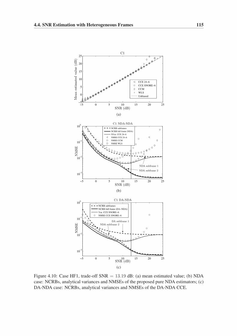
4.4. SNR Estimation with Heterogeneous Frames 115
−5 0 5 10 15 20 25−5
0
5
10
15
20
25
SNR (dB)
Mea
nes
tim
ate
dva
lue
(dB
)
C1
CCE 24−6
CCE SNORE−6
CCM
WLS
Unbiased
(a)
−5 0 5 10 15 20 25
10−3
10−2
10−1
100
SNR (dB)
NM
SE
C1 NDA-NDA
NDA subframe 1
NDA subframe 2
NCRB subframes
NCRB full frame (NDA)
NVar. CCE 24−6
NMSE CCE 24−6
NMSE CCM
NMSE WLS
(b)
−5 0 5 10 15 20 25
10−3
10−2
10−1
100
SNR (dB)
NM
SE
C1 DA-NDA
DA subframe 1NDA subframe 2
NCRB subframes
NCRB full frame (DA−NDA)
Var. CCE SNORE−6
NMSE CCE SNORE−6
(c)
Figure 4.10: Case HF1, trade-off SNR = 13.19 dB: (a) mean estimated value; (b) NDA
case: NCRBs, analytical variances and NMSEs of the proposed pure NDA estimators; (c)
DA-NDA case: NCRBs, analytical variances and NMSEs of the DA-NDA CCE.

116 Chapter 4. SNR Estimation
bias above SNR = 16 dB, while both CCE estimators and the WLS estimator present no
noticeable bias between 0 and 20 dB. Figure 4.10b displays the case of combination of two
NDA estimates. Shown are the NDA NCRBs for each subframe and for the heterogeneous
frame, as well as the analytical variance of the NDA-NDA CCE of ρ(1)24 , ρ
(2)6 . Finally,
we show also the NMSE obtained through simulations for the NDA-NDA CCE estimator
(λtrade-offcce,24−6 = 0.3339), the CCM estimator (λccm,2 = 0.2069, λccm,4 = 0.2254), and the WLS
estimator (w1 = 0.85). The former weights have been calculated taking SNR = 13.19 dB
as a reference [marked as a vertical solid line in Figures 4.10b and 4.10c]. Figure 4.10c
displays the DA-NDA case. We show the DA NCRB over the Kt training symbols, the
NDA NCRB over subframe 2, and the joint DA-NDA NCRB. We also show the analytical
variance of the DA-NDA CCE ρ(1)DA-ML, ρ
(2)6 , as well as the empirical NMSE obtained for
the DA-NDA CCE with λtrade-offcce,DA-ML−6 = 0.3865.
It is remarkable that both the NDA-NDA and the DA-NDA full-frame NCRBs are
close to the NDA NCRBs over subframe 2, especially for moderate to high SNRs; this
means that the higher number of samples in subframe 2 is more statistically meaningful
than the few QPSK symbols (or training symbols) of subframe 1. We can also observe
that both CCE estimators perform close to their minimum variance not only for the SNR
of reference but also for a wide range of SNRs. The CCE of DA-ML and ρ6 performs
slightly better than the CCE of ρ24 and ρ6, which is explained due to the lower variance
of the DA estimator with respect to the NDA estimator over subframe 1. Both CCE
estimators depart from the NCRB for SNRs above 10 dB, similarly to the behavior of the
constituent estimator ρ6.
Figure 4.11 presents the same results as Figure 4.10 but for case HF2. The estima-
tors have been simulated considering the reference SNR = 10.62 dB [marked as a ver-
tical solid line in Figures 4.11b and 4.11c], for which the following parameters were
obtained: λtrade-offcce,24−6 = 0.2632, λtrade-off
cce,DA-ML−6 = 0.3259, λccm,2 = 0.2038, λccm,4 = 0.1919,
and w1 = 0.3. Roughly speaking, the same comments made for case HF1 apply for case
HF2. Among the differences, we note the bias of the WLS estimator above 18 dB, while
both CCE estimators can be considered unbiased between 0 and 25 dB. Also, unlike in
HF1, here the WLS performs similarly to CCM in terms of NMSE. However, both CCE
estimators show again the lowest NMSE. This is due to ρ6, which outperforms the esti-
mators over subframe 2 because it is well suited to the 16-APSK constellation (notice that
the gap between NCRB and NMSE of CCE is smaller for case HF2 than for case HF1).
In general, our results show that the CCE approach consistently outperforms the CCM
and WLS approaches. The limitation of the CCM and WLS approaches lies in the fact that
they are restricted to using only second and fourth order statistics. Therefore, they cannot
be expected to perform well with multilevel constellations, as shown in our results. On the
other hand, the CCE approach is not bound to use a particular estimator; instead, any pair
of (unbiased) estimators can be combined to yield a new estimator with lower variance
(under an appropriate choice of λcce). This includes DA schemes, which turns into a
further advantage of the CCE scheme when training symbols (pilots, partially known
header) are available in the heterogeneous frame.. The two considered CCE estimators
perform well over a wide SNR range; in particular, the hybrid DA-NDA CCE estimator
performs slightly better than the NDA-NDA estimator, which is explained by the lower

4.4. SNR Estimation with Heterogeneous Frames 117
−5 0 5 10 15 20 25−5
0
5
10
15
20
25
SNR (dB)
Mea
nes
tim
ate
dva
lue
(dB
)
C2
CCE 24−6
CCE SNORE−6
CCM
WLS
Unbiased
(a)
−5 0 5 10 15 20 25
10−3
10−2
10−1
100
SNR (dB)
NM
SE
C2 NDA-NDA
NDA subframe 1
NDA subframe 2
NCRB subframes
NCRB full frame (NDA)
NVar. CCE 24−6
NMSE CCE 24−6
NMSE CCM
NMSE WLS
(b)
−5 0 5 10 15 20 25
10−3
10−2
10−1
100
SNR (dB)
NM
SE
C2 DA-NDA
DA subframe 1
NDA subframe 2
NCRB subframes
NCRB full frame (DA−NDA)
Var. CCE SNORE−6
NMSE CCE SNORE−6
(c)
Figure 4.11: Case HF2, trade-off SNR = 10.62 dB: (a) mean estimated value; (b) NDA
case: NCRBs, analytical variances and NMSEs of the proposed pure NDA estimators; (c)
DA-NDA case: NCRBs, analytical variances and NMSEs of the DA-NDA CCE.

118 Chapter 4. SNR Estimation
variance of the DA estimator over subframe 1.

4.A. SNR Estimation Using Higher-Order Moments 119
Appendix 4.A SNR Estimation Using Higher-Order Mo-
ments
In this appendix section we provide the proofs of the results given in Section 4.3.
4.A.1 Proof of Property 1
Recalling (4.5), it is possible to write the numerator and denominator of (4.9) as
U∏
i=1
Mpi2ni
= NQD(ρ) (4.56)
MQ2 = NQ(1 + ρ)Q (4.57)
with D(ρ) a polynomial of degree Q. As expected, the ratio of (4.56) to (4.57) does not
depend on N . Now, applying the change of variable ρ = z/(1−z), one has ρm/(1+ρ)Q =zm(1− z)Q−m, for m = 0, 1, . . . , Q, which shows that
f(ρ) =
Q∑
m=0
Dm zm(1− z)Q−m = F (z) (4.58)
is a polynomial of degree Q in z. We note that this property holds also for any linear
combination of ratios of the form of (4.9). We will prove now that F1, the coefficient in zof F (z) = f(ρ), is always zero. Since f(ρ) is a product of terms of the form M2n/M
n2 , it
suffices to show that any such term is a polynomial in z with zero first-order coefficient.
To see this, note from (4.5) and ρ = z/(1−z) that M2n/Mn2 =
∑nm=0 G
(n)m zm(1−z)n−m,
where G(n)m
.= c2m(n!)
2/[(n−m)!(m!)2]. Since zm(1−z)n−m = zm−(n−m)zm+1+ · · · ,
it follows that the coefficient in z of M2n/Mn2 is G
(n)1 − nG
(n)0 = n(n!)c2 − n(n!)c0 = 0,
since c0 = c2 = 1.
4.A.2 Computation of the Variance (4.20)
From the definitions of t(m), g(m) and hEOS(m) we have
∇t =∇g
(1− g)2(4.59)
∇g =∇hEOS
F ′EOS
(g)=
∇hEOS
4F4 g3 + 3F3 g2 + 2F2 g. (4.60)
∇hEOS can be readily computed from (4.13), obtaining
∇hEOS =1
M52
Rα (4.61)
R.=
−2M4M22 −3M6M2 −4M2
4 −4M8
M32 0 2M4M2 0
0 M22 0 0
0 0 0 M2
. (4.62)

120 Chapter 4. SNR Estimation
Now, noting that g|m=m = z = ρ/(1 + ρ), the evaluation of (4.59)–(4.62) at m = m
yields
v =1
N5
Rα
X(ρ)(4.63)
where R.= R|m=m. The polynomial X(ρ)
.= X3 ρ
3+X2 ρ2+X1 ρ is linear in α: we can
write X3.= 4F4+3F3+2F2 = αTx3, X2
.= 3F3+4F2 = αTx2, and X1
.= 2F2 = αTx1,
where the 4 × 1 vectors x1, x2, x3 depend on the constellation moments only. Upon
defining x(ρ).=∑3
n=1 xn ρn, one has that X(ρ) = αTx(ρ), and the approximation of
the variance can be written as
vTCv =1
N10
αTRTCRα
αTx(ρ)[x(ρ)]Tα. (4.64)
Observe that [C]ij = (M2(i+j) −M2iM2j)/K has the form of (4.56) for Q = i + j, and
that the elements of the i-th row of R have the form of (4.56) as well, with Q = 5 − i,(i = 1, 2, 3, 4). It is then possible to show that all the nonzero elements of RTCR are of
the form of (4.56) with Q = 10. With this, the factor N10 in (4.64) cancels out and (4.20)
follows by simply identifying A(Var)(ρ) = K/N10 αTRTCRα, and B(Var)(ρ) = X2(ρ) =αTx(ρ)[x(ρ)]Tα, which are polynomials in ρ of degrees 10 and 6 respectively.
4.A.3 Proofs of Properties 2–5
That B(Var)(ρ) has rank one (Property 4) is evident from (4.64), if we identify x(ρ)[x(ρ)]T
with B(Var)(ρ) of (4.40) [and therefore x(ρ) = b(Var)(ρ)]. Similarly, identifying b(Var)6 with
x3, so that B(Var)6 = x3x
T3 , then Property 5 follows.
In order to prove that A(Var)(ρ) is rank deficient (Property 2), we note that R has
rank 3 since its first and third columns are linearly dependent, see (4.62). It follows that
rank(A(Var)(ρ)
)= rank
(RTCR
)≤ 3 for all ρ. The first part of Property 3 immediately
follows by noting that A(Var)10 = limρ→∞ A(Var)(ρ)/ρ10. Finally, for constellations with
I = 1, 2 or 3 amplitude levels, it is straightforward (but rather tedious) to explicitly
compute A(Var)10 , as well as to check that its rank does not exceed 0, 1, and 2, respectively.
4.A.4 Computation of the Bias (4.24)
The Hessian matrix of t(m), ∇2t, can be readily computed from (4.59)–(4.61) as
∇2t =1
(1− g)2F ′EOS
(g)∇2h
+2F ′
EOS(g)− (1− g)F ′′
EOS(g)
(1− g)3[F ′EOS
(g)]2∇h (∇h)T (4.65)
=1
(1− g)2F ′EOS
(g)
1
M62
Y + Jt(g)∇t (∇t)T (4.66)

4.A. SNR Estimation Using Higher-Order Moments 121
where
Jt(g).=
(1− g) [2F ′EOS
(g)− (1− g)F ′′EOS
(g)]
F ′EOS
(g)(4.67)
and Y is a 4× 4 symmetric matrix whose only nonzero elements are given by
[Y ]11.= 6βM4M
22 + 12γM6M2 + 20(δM2
4 + ǫM8) (4.68a)
[Y ]12 = [Y ]21.= −2βM3
2 − 8δ M4M2 (4.68b)
[Y ]13 = [Y ]31.= −3γM2
2 (4.68c)
[Y ]14 = [Y ]41.= −4ǫM2 (4.68d)
[Y ]22.= 2δM2
2 . (4.68e)
The evaluation of (4.66) at m = m yields
H.= ∇2t|m=m =
1
N6
1
(1 + ρ)X(ρ)Y + 2J(ρ) vvT (4.69)
where Y = Y |m=m, X(ρ) has been defined in Section 4.A.2 of this Appendix, and
J(ρ).= 1
2Jt(
ρ1+ρ
). Regarding the first term of (4.69), its denominator is clearly linear in
α: (1 + ρ)X(ρ) = αT[(1 + ρ)x(ρ)], from where we can identify b(L)(ρ) of (4.26) as
b(L)(ρ) = (1 + ρ)x(ρ) = (1 + ρ)b(Var)(ρ). (4.70)
Regarding the factor J(ρ) in second term of (4.69), it is readily seen to be of the form
J(ρ) = A(J)(ρ)/[(1+ρ)X(ρ)] = [αTa(J)(ρ)]/[αTb(L)(ρ)], where A(J)(ρ).=∑3
n=0A(J)n ρn =
αTa(J)(ρ), and a(J)(ρ) depends on ρ and the constellation moments.
Recalling the approximation (4.23), simple algebra shows that
1
2Tr (H C) =
1
2
Tr (Y C)
N6 (1 + ρ)X(ρ)+ J(ρ)vTCv (4.71)
where the second term turns out to be proportional to the approximation for the vari-
ance (4.18). Using (4.20)-(4.22) and (4.70) we can write the second term of (4.71) as a
quotient of cubic forms in α:
J(ρ) vTCv =1
K
αTa(J)(ρ)αTA(Var)(ρ)α
(1 + ρ)[αTb(Var)(ρ)]3. (4.72)
As for the computation of the first term of (4.71), which amounts to L(ρ) in (4.24a),
observe that the nonzero [Y ]ij have the form of (4.56) with Q = 6 − (i + j). We are
eventually interested in the elements of the diagonal of HC, which are given by
[HC]ii =
∑4j=1 [Y ]ij [C]ji
N6(1 + ρ)X(ρ)(4.73)
for i = 1, 2, 3, 4. All terms([Y ]ij [C]ji
)have then the form of (4.56) with Q = 6.
Clearly, N6 cancels out in (4.73), so that the first term in (4.24) follows if we iden-
tify L(ρ) = A(L)(ρ)/B(L)(ρ), where A(L)(ρ) = K∑4
i=1
∑4j=1 [Y ]ij [C]ji /(2N
6) and
B(L)(ρ) = (1+ρ)X(ρ). Besides, A(L)(ρ) can be readily seen to be linear in α, since it is a
linear combination of the elements of Y , which are themselves linear in α [cf. (4.66)]; this
allows to write A(L)(ρ) =∑6
n=0A(L)n ρn = αTa(L)(ρ) as in (4.25), for some a(L)(ρ) =
∑6n=0 a
(L)n ρn, in which a
(L)n depends only on the constellation moments for all n.

122 Chapter 4. SNR Estimation
Appendix 4.B Generalization: SNR Estimation from Ra-
tios of Moments of Any Order
The approach to SNR estimation developed in Section 4.3 is based on ratios of moments
of the form of (4.9). Such ratios are built with exclusively even-order moments in the
numerator and M2 in the denominator. Such moment selection allows to develop SNR es-
timators with the desirable feature that they can be implemented avoiding LUTs via some
root-finding algorithm. If we drop this feature, i.e., if we allow LUTs in the implemen-
tation, then a wider choice of ratios is available for estimator design. For example one
could try to develop estimators based on linear combinations of ratios of the family (4.6)
proposed in [68]. However, a more general family can be considered.
In this Appendix we propose the development of SNR estimators based on of ratios of
moments of the following form
f(ρ) =
U∏
k=1
Mr(k)p(k)
V∏
k=1
Ms(k)q(k)
such that (4.74a)
2Q.=
U∑
k=1
p(k)r(k) =V∑
k=1
q(k)s(k) (4.74b)
where we maintain the notation “2Q” used in Section 4.3 to denote the statistical order
of numerator and denominator, which must be the same in order to ensure that the noise
power N cancels out in the ratio [recall (4.4)]. Without loss of generality, we will assume
that the numerator and denominator of (4.74) do not feature common moments, and that
p(k) 6= p(j), q(k) 6= q(j) for k 6= j. Therefore (4.74) features a total of U + V different
moments. We note that the moment orders p(k) and q(k) can be odd. Examples of ratios
belonging to this family are
M1M3
M22
(2Q = 4),M3M2
M1M4
(2Q = 5),M5M3
M4M2M21
(2Q = 8), . . .
The family of ratios (4.74) represents a general form which includes the ratios (4.6)
and (4.9) as particular cases. The number of possible ratios within a given statistical
order increases considerably with respect to those subfamilies. Table 4.2 shows this by
comparing the total number of possible ratios within each (sub)family for each statistical
order up to eighth-order. This fact represents a potential improvement over the family
analyzed in Section 4.3: one can build a potentially competitive SNR estimator without
moving to high statistical orders. For example, if we allow up to the third statistical order
(2Q ≤ 3) we have the following:
(i) there are no available ratios of the form of (4.9);
(ii) the family (4.6) offers four ratios: M2/M21 , M3/M
31 , and their inverses;

4.B. Generalization: SNR Estimation from Ratios of Moments of Any Order 123
Table 4.2: Number of existing ratios in the family (4.74), and the subfamilies (4.6)
from [68], and (4.9)
Number of existing ratios*
Order 2Q(4.74) (4.6) (4.9)
2 2 2 0
3 4 2 0
4 12 2 1
5 16 2 0
6 48 4 1
7 56 2 0
8 134 4 2
*A ratio and its inverse are considered as different ratios
except for the subfamily (4.9).
(iii) the general family (4.74) offers six ratios: M2/M21 , M3/M
31 , M3/(M1M2) and their
inverses.
We propose to estimate the SNR ρ using a linear combination of the form
f(ρ) = α1f1(ρ) + α2f2(ρ) + . . .+ αtft(ρ)
= αTf(ρ) (4.75)
with α.= [α1 α2 . . . αt]
T a vector of t real-valued weights, and f(ρ).= [f1(ρ) f2(ρ) . . . ft(ρ)]
T
the vector of the t ratios of moments belonging to the family (4.74). Similarly to Sec-
tion 4.3.3, we introduce the vector of true moments m.= [m1 m2 . . . mµ]
T containing
the µ different moments appearing in (4.75) (m is the corresponding vector of sample
moments), and the function h(m) = α1h1(ρ) + α2h2(ρ) + . . . + αtht(ρ).= f(ρ) which
considers the moments as the independent variables in (4.75). The SNR estimate is then
given by
ρ = f−1(h(m)) (4.76)
with f−1(·) the inverse of (4.75), which in general will not have a closed-form (and thus
the need of an LUT for implementing it).
Example For illustrative reasons, consider the linear combination of all ratios up to
order three
f(ρ) = α1M2
M21
+ α2M2
1
M2
+ α3M3
M31
+ α4M3
1
M3
+ α5M3
M1M2
+ α6M1M2
M3
. (4.77)
We identify t = 6 (number of ratios), m = [M1 M2 M3]T (and hence µ = 3), and
the obvious definition of the vector of ratios f(ρ). Considering the last ratio f6(ρ) =(M1M2)/M3, comparison with (4.74) allows to identify U = 2, V = 1, p(1) = 1,
p(2) = 2, q(1) = 3, and r(1) = r(2) = s(1) = 1.

124 Chapter 4. SNR Estimation
4.B.1 Statistical Analysis
We briefly sketch the statistical analysis of the proposed estimator (4.76), which pro-
ceeds similarly to the analysis performed in Section 4.3.3. Let us first define the function
g(m).= f−1(h(m)) = ρ, whose implicit definition is given by f(g) = h(m).
Variance We approximate the variance through Var {ρ} ≈ vTCv, see (4.18), where in
this case v.= ∇g|m=m and C is the covariance matrix of m. After some algebraic steps
it is found that
∇g =∇h
f ′(g)(4.78)
∇h = Rα (4.79)
with R a µ× t matrix with elements [R]ij = ∂hj/∂mi. Hence,
v =Rα
f ′(ρ)(4.80)
with R.= R|m=m, so the approximate variance eventually results in
Var {ρ} ≈ αTRTCRα
[f ′(ρ)]2. (4.81)
Note that, similarly to (4.20), the variance is a quotient of quadratic forms in α,11 which
is inversely proportional to the observation length K (due to C).
Bias Recalling (4.23), the bias is approximated by Bias {ρ} ≈ 12Tr (HC), with H
.=
∇2g|m=m. After some algebra, and using the definitions Y.= ∇2h and Y
.= Y |m=m it
is found that
∇2g =1
f ′(g)Y − f ′′(g)
f ′(g)∇g(∇g)T (4.82)
H =1
f ′(ρ)Y − f ′′(g)
f ′(g)vvT. (4.83)
With this, the approximation of the bias reads
Bias {ρ} ≈ 1
2
Tr (Y C)
f ′(ρ)− 1
2
f ′′(ρ)
f ′(ρ)Var {ρ} (4.84)
which shares the structure of the approximation (4.24): the first term is a quotient of linear
forms in α, and the second one is a quotient of cubic forms in α.
11Since f(ρ) is linear in α, see (4.75), and so is f ′(ρ).

4.C. SNR Estimation with Heterogeneous Frames 125
Weight optimization The optimization of the weight vector α must be performed for
each particular linear combination of ratios. In any case, the principles that inspired the
optimization criteria proposed in Section 4.3.4, and the mathematical tools used therein
are valid in this case as well.12 The only difference with respect to the estimators pro-
posed in Section 4.3 is that, in general, the elements of the vectors and matrices involved
in (4.81) and (4.84) will not be polynomials in ρ, but more complicated functions of ρ.
This fact may yield the optimization procedure somewhat more cumbersome. Intuitively,
increasing t (number of ratios in the linear combination) should translate into a perfor-
mance improvement in terms of MSE.13 Based on this, the proposed family of estimators
has the potential to outperform the eight-order estimator of Section 4.3 with statistics of
lower order. However, this is a conjecture that needs corroboration, and is left here as a
future research line.
Appendix 4.C SNR Estimation with Heterogeneous Frames
4.C.1 A Suboptimal Approach to Weight Selection for the CCM Es-
timator
A simpler, suboptimal approach is to choose λccm,n so as to minimize the variance of
M ccmn , since this should intuitively translate into a smaller variance of ρccm
24 . The variance
of the combined moments is given by
Var{
M ccmn
}
= λ2ccm,n
(σ(1)n
)2+ (1− λccm,n)
2(σ(2)n
)2(4.85)
where the variances in the right hand side are those of the constituent sample moments,
and are given by
(σ(i)n
)2 .= Var
{
M (i)n
}
=[M
(i)2n −
(M (i)
n
)2]/Ki. (4.86)
With this we find that the value minimizing (4.85) is given by
λccm,n =
(σ(1)n
)2
(σ(1)n
)2+(σ(2)n
)2 . (4.87)
Notice the similarity with (4.48). For n = 2, 4 the variance ratios in (4.87) equal
(σ(1)2
)2
(σ(2)2
)2 =K2
K1
A(1)(ρ)
A(2)(ρ),
(σ(1)4
)2
(σ(2)4
)2 =K2
K1
B(1)(ρ)
B(2)(ρ)(4.88)
12The actual optimization criterion must be tailored to each particular case, considering the number of
scalar weights available for optimization.13Recall that the dimension t of the weight vector α represents in fact t− 1 degrees of freedom available
for estimator design, since the variance (4.81) and the bias (4.84) are invariant under scalings in α.

126 Chapter 4. SNR Estimation
where
A(i)(ρ).=[c(i)4 −
(c(i)2
)2]ρ2 + 2c
(i)2 ρ+ 1, (4.89)
B(i)(ρ).=[c(i)8 −
(c(i)4
)2]ρ4 + 8
[2c
(i)6 − c
(i)2 c
(i)4
]ρ3
+[68c
(i)4 − 16
(c(i)2
)2]ρ2 + 80c
(i)2 ρ+ 80. (4.90)
Notice that for low SNR values both quotients in (4.88) approach 1, which leads to
λccm,n ≈ K1/(K1 +K2) = p. On the other hand, for high SNR the terms in ρ2 (resp. ρ4)dominate in A(i)(ρ) [resp. B(i)(ρ)], and thus λccm,n ≈ K1/(K1 + αnK2), where
αn.=
c(1)2n −
(c(1)n
)2
c(2)2n −
(c(2)n
)2 for n = 2, 4.

Chapter 5Phase Estimation for Cross-QAM
Constellations
Contents
5.1 Introduction . . . . . . . . . . . . . . . . . . . . . . . . . . . . . . . 127
5.2 System Model and Classical Estimators . . . . . . . . . . . . . . . . 130
5.3 Phase Estimation Based on ℓ1-norm Maximization . . . . . . . . . . 131
5.4 Fixed Point Iterations for Phase Estimation . . . . . . . . . . . . . . 133
5.4.1 Maximization of J1(θ) . . . . . . . . . . . . . . . . . . . . . . 134
5.4.2 Maximization of J2(θ) . . . . . . . . . . . . . . . . . . . . . . 134
5.5 Discussion and Statistical Analysis . . . . . . . . . . . . . . . . . . . 135
5.5.1 Algorithm Initialization . . . . . . . . . . . . . . . . . . . . . 135
5.5.2 Computational Complexity . . . . . . . . . . . . . . . . . . . . 136
5.5.3 Asymptotic Variances . . . . . . . . . . . . . . . . . . . . . . 136
5.6 Simulation Results . . . . . . . . . . . . . . . . . . . . . . . . . . . . 137
5.6.1 Floating Point Precision . . . . . . . . . . . . . . . . . . . . . 138
5.6.2 Fixed Point Implementation . . . . . . . . . . . . . . . . . . . 139
Appendix 5.A Phase Estimation Based on ℓ∞-norm . . . . . . . . . . . . 144
Appendix 5.B Proof of Theorem 1 . . . . . . . . . . . . . . . . . . . . . 145
5.1 Introduction
Carrier phase recovery is a key element in bandpass digital communication receivers.
Many authors have addressed this topic over the last years, yielding a wide variety of
recovery methods depending on the modulation scheme and application constraints [76,
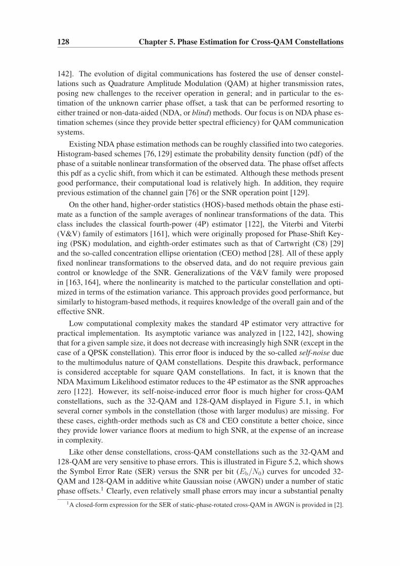
128 Chapter 5. Phase Estimation for Cross-QAM Constellations
142]. The evolution of digital communications has fostered the use of denser constel-
lations such as Quadrature Amplitude Modulation (QAM) at higher transmission rates,
posing new challenges to the receiver operation in general; and in particular to the es-
timation of the unknown carrier phase offset, a task that can be performed resorting to
either trained or non-data-aided (NDA, or blind) methods. Our focus is on NDA phase es-
timation schemes (since they provide better spectral efficiency) for QAM communication
systems.
Existing NDA phase estimation methods can be roughly classified into two categories.
Histogram-based schemes [76, 129] estimate the probability density function (pdf) of the
phase of a suitable nonlinear transformation of the observed data. The phase offset affects
this pdf as a cyclic shift, from which it can be estimated. Although these methods present
good performance, their computational load is relatively high. In addition, they require
previous estimation of the channel gain [76] or the SNR operation point [129].
On the other hand, higher-order statistics (HOS)-based methods obtain the phase esti-
mate as a function of the sample averages of nonlinear transformations of the data. This
class includes the classical fourth-power (4P) estimator [122], the Viterbi and Viterbi
(V&V) family of estimators [161], which were originally proposed for Phase-Shift Key-
ing (PSK) modulation, and eighth-order estimates such as that of Cartwright (C8) [29]
and the so-called concentration ellipse orientation (CEO) method [28]. All of these apply
fixed nonlinear transformations to the observed data, and do not require previous gain
control or knowledge of the SNR. Generalizations of the V&V family were proposed
in [163, 164], where the nonlinearity is matched to the particular constellation and opti-
mized in terms of the estimation variance. This approach provides good performance, but
similarly to histogram-based methods, it requires knowledge of the overall gain and of the
effective SNR.
Low computational complexity makes the standard 4P estimator very attractive for
practical implementation. Its asymptotic variance was analyzed in [122, 142], showing
that for a given sample size, it does not decrease with increasingly high SNR (except in the
case of a QPSK constellation). This error floor is induced by the so-called self-noise due
to the multimodulus nature of QAM constellations. Despite this drawback, performance
is considered acceptable for square QAM constellations. In fact, it is known that the
NDA Maximum Likelihood estimator reduces to the 4P estimator as the SNR approaches
zero [122]. However, its self-noise-induced error floor is much higher for cross-QAM
constellations, such as the 32-QAM and 128-QAM displayed in Figure 5.1, in which
several corner symbols in the constellation (those with larger modulus) are missing. For
these cases, eighth-order methods such as C8 and CEO constitute a better choice, since
they provide lower variance floors at medium to high SNR, at the expense of an increase
in complexity.
Like other dense constellations, cross-QAM constellations such as the 32-QAM and
128-QAM are very sensitive to phase errors. This is illustrated in Figure 5.2, which shows
the Symbol Error Rate (SER) versus the SNR per bit (Eb/N0) curves for uncoded 32-
QAM and 128-QAM in additive white Gaussian noise (AWGN) under a number of static
phase offsets.1 Clearly, even relatively small phase errors may incur a substantial penalty
1A closed-form expression for the SER of static-phase-rotated cross-QAM in AWGN is provided in [2].
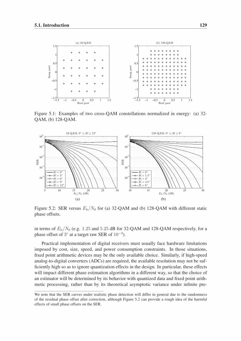
5.1. Introduction 129
−1.5 −1 −0.5 0 0.5 1 1.5−1.5
−1
−0.5
0
0.5
1
1.5
Real part
Imag
part
(a) 32-QAM
−1.5 −1 −0.5 0 0.5 1 1.5−1.5
−1
−0.5
0
0.5
1
1.5
Real part
Imag
part
(b) 128-QAM
Figure 5.1: Examples of two cross-QAM constellations normalized in energy: (a) 32-
QAM, (b) 128-QAM.
5 10 15 20 25 30
10−4
10−3
10−2
10−1
100
Eb/N0 (dB)
SE
R
32-QAM, 0◦ ≤ |θ| ≤ 12◦
|θ| = 0◦
|θ| = 3◦
|θ| = 6◦
|θ| = 9◦
|θ| = 12◦
(a)
10 15 20 25 30
10−4
10−3
10−2
10−1
100
Eb/N0 (dB)
SE
R
128-QAM, 0◦ ≤ |θ| ≤ 6◦
|θ| = 0◦
|θ| = 1.5◦
|θ| = 3◦
|θ| = 4.5◦
|θ| = 6◦
(b)
Figure 5.2: SER versus Eb/N0 for (a) 32-QAM and (b) 128-QAM with different static
phase offsets.
in terms of Eb/N0 (e.g. 1.25 and 5.25 dB for 32-QAM and 128-QAM respectively, for a
phase offset of 3◦ at a target raw SER of 10−3).
Practical implementation of digital receivers must usually face hardware limitations
imposed by cost, size, speed, and power consumption constraints. In those situations,
fixed point arithmetic devices may be the only available choice. Similarly, if high-speed
analog-to-digital converters (ADCs) are required, the available resolution may not be suf-
ficiently high so as to ignore quantization effects in the design. In particular, these effects
will impact different phase estimation algorithms in a different way, so that the choice of
an estimator will be determined by its behavior with quantized data and fixed point arith-
metic processing, rather than by its theoretical asymptotic variance under infinite pre-
We note that the SER curves under realistic phase detection will differ in general due to the randomness
of the residual phase offset after correction, although Figure 5.2 can provide a rough idea of the harmful
effects of small phase offsets on the SER.

130 Chapter 5. Phase Estimation for Cross-QAM Constellations
cision. Although estimation performance is difficult to analyze under finite wordlength
constraints, intuitively one would expect that estimators requiring fewer, lower-order op-
erations on the observed data be more robust in these situations. For example, the per-
formance of the 4P phase estimate is expected to degrade more gracefully than that of
eighth-order methods such as C8 and CEO.
These considerations motivate the search for low-complexity NDA phase estimators
for cross-QAM systems. In this chapter we develop two such schemes by maximizing
certain cost functions arising from geometrical considerations based on the square-like
shape of QAM constellations. Although it is not possible to derive closed-form expres-
sions for these maximizers, we present simple iterations which locally converge to the
desired values, and which can be initialized by any suitable scheme providing a coarse
phase estimate. The choice of the initializer should be tailored to the operation environ-
ment (constellation size, number of samples, availability of training data, etc.).
Chapter structure The chapter is organized as follows. Section 5.2 presents the signal
model and reviews the classical one-shot estimators that will be considered in the chapter.
Maximization of the ℓ1-norm as a criterion for phase estimation is justified in Section 5.3,
whereas the two proposed estimators are derived in Section 5.4. Section 5.5 provides
an analysis in terms of variance, initialization and computational complexity. Simulation
results, for both floating point and fixed point implementations, are shown in Section 5.6,
and conclusions are drawn in Section 6.1. The contents of this chapter derive from the
work presented in [5, 8].
5.2 System Model and Classical Estimators
Consider the receiver of QAM system, in which the received signal is sampled at the
baud rate after front-end processing. Assuming that carrier frequency recovery has been
previously established, the observed data can be written as
rk = akejθ + nk, k = 0, 1, . . . , L− 1 (5.1)
where {ak} are the transmitted symbols, drawn equiprobably from a constellation A with
size M and variance Ea, and {nk} are the complex-valued noise samples. The noise is
assumed zero-mean, circular white Gaussian with variance σ2, and independent of the
symbols. The phase offset θ is assumed to vary slowly; thus, it can be taken as constant
within the block of L samples. The goal is to identify θ without knowledge of the symbols
ak or the variances Ea, σ2. Due to the quadrant symmetry of QAM constellations, this
phase offset can only be blindly identified up to a four-fold ambiguity; hence, we assume
that |θ| < π/4.
The V&V family of estimators [161] embraces a wide range of choices. Of particular
interest are power-law estimators
θVV-p =1
4arg
{
−L−1∑
k=0
|rk|pej4arg{rk}
}
(5.2)

5.3. Phase Estimation Based on ℓ1-norm Maximization 131
where p is an integer. For p = 0, the corresponding estimate θVV-0 discards the envelope
information of the received signal. On the other hand, for p = 4 one obtains the 4P
estimator [122, 142]:
θ4P =1
4arg
{
−L−1∑
k=0
r4k
}
. (5.3)
Several alternatives have been proposed to improve the performance of the 4P method
with cross-QAM constellations. One of them advocates the use of (5.2) with negative
values of p, although the resulting estimators are competitive in the high SNR regime
only [31]. An alternative approach with better performance at lower SNRs is Cartwright’s
eighth-order estimator [29]
θC8 =1
4tan−1
∑
k
AkBk
∑
l
AlCl −∑
k
A2k
∑
l
BlCl
∑
k
AkBk
∑
l
BlCl −∑
k
B2k
∑
l
AlCl
(5.4)
where Ak.= Re {r4k}, Bk
.= Im {r4k} and Ck
.= |rk|4, and all summations in k and l
in (5.4) run from 0 to L − 1. We note that the four quadrant inverse tangent function
is required in (5.4). The price to pay for the reduced variance of (5.4) with respect to
that of (5.3) is a higher computational load. A different eighth-order estimator (CEO)
was proposed in [28]; its computational complexity and performance with cross-QAM
constellations are similar to those of (5.4).
5.3 Phase Estimation Based on ℓ1-norm Maximization
Consider the mapping f : C → R2 that assigns to each complex number z = z + jz
the real vector z.= f(z) = [z z]T. Under f , multiplication by a phase term ejθ in
C becomes multiplication by an orthogonal rotation matrix in R2. Given a candidate
estimate θ, let us define the de-rotated samples
yk = e−jθrk = yk + jyk (5.5)
and consider the effect of such de-rotation on the vector yk = f(yk) = [yk yk]T. In
particular, we focus on the resulting ℓ1-norm of the phase-compensated vector
||yk||1 = |yk|+ |yk|. (5.6)
We claim that maximization of the ℓ1-norm with respect to θ is a meaningful criterion
for obtaining a phase estimate with QAM constellations. To see this, it is instructive to
consider the geometry of the simplest case, i.e. a QPSK constellation (M = 4) A ={√Eae
j(π4+nπ
2), 0 ≤ n ≤ 3} in the noiseless case. Recall that the ℓ1-ball defined by
||y||1 = γ is a diamond with corners at [0 ±γ]T and [±γ 0]T. It is clear from Figure 5.3
that any rotation of A by an angle that is not of the form nπ/2 with n integer can only
result in a smaller average ℓ1-norm of the rotated constellation. That is, the ℓ1-norm is

132 Chapter 5. Phase Estimation for Cross-QAM Constellations
Figure 5.3: Effect of a rotation on the average ℓ1-norm of a QPSK constellation. Solid
dots: original constellation; empty dots: rotated constellation.
maximized when the positioning of the constellation is restored to its original regular
grid.
Observe that for QPSK the average ℓ1-norm of the constellation coincides with the
ℓ1-norm of any of its elements, for all phase offsets. This is because this constellation can
be obtained by picking any of its elements and all possible rotations by an integer multiple
of π/2 rad, and the ℓ1-norm is preserved by these operations, as it can be easily checked.2
For larger constellations this property does not hold anymore, although it can be checked
that the average ℓ1-norm still attains its maximum for a zero phase offset in absence of
noise. This is shown in Figures 5.4 and 5.5, which plot the cost functions
−40 −20 0 20 400.75
0.8
0.85
0.9
0.95
1
phase error (deg)
16-QAM
−40 −20 0 20 400.75
0.8
0.85
0.9
0.95
1
phase error (deg)
64-QAM
−40 −20 0 20 400.75
0.8
0.85
0.9
0.95
1
phase error (deg)
256-QAM
−40 −20 0 20 400.75
0.8
0.85
0.9
0.95
1
phase error (deg)
1024-QAM
Figure 5.4: Square QAM constellations: behavior of the ℓ1-norm based cost functions
Jq(θ) (normalized to their maximum value) in absence of noise. q = 1 (solid) and 2(dashed).
Jq(θ).= E {||y||q1} = E {(|y|+ |y|)q} (5.7)
2Conjugation is another ℓ1-norm-preserving operation.
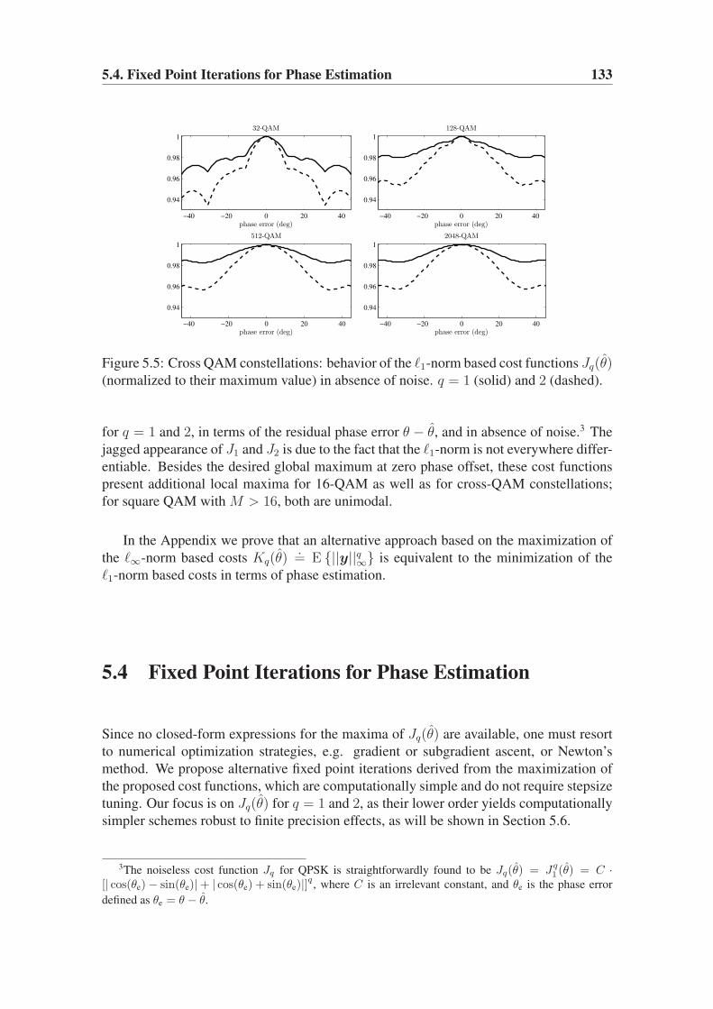
5.4. Fixed Point Iterations for Phase Estimation 133
−40 −20 0 20 40
0.94
0.96
0.98
1
phase error (deg)
32-QAM
−40 −20 0 20 40
0.94
0.96
0.98
1
phase error (deg)
128-QAM
−40 −20 0 20 40
0.94
0.96
0.98
1
phase error (deg)
512-QAM
−40 −20 0 20 40
0.94
0.96
0.98
1
phase error (deg)
2048-QAM
Figure 5.5: Cross QAM constellations: behavior of the ℓ1-norm based cost functions Jq(θ)(normalized to their maximum value) in absence of noise. q = 1 (solid) and 2 (dashed).
for q = 1 and 2, in terms of the residual phase error θ − θ, and in absence of noise.3 The
jagged appearance of J1 and J2 is due to the fact that the ℓ1-norm is not everywhere differ-
entiable. Besides the desired global maximum at zero phase offset, these cost functions
present additional local maxima for 16-QAM as well as for cross-QAM constellations;
for square QAM with M > 16, both are unimodal.
In the Appendix we prove that an alternative approach based on the maximization of
the ℓ∞-norm based costs Kq(θ).= E {||y||q∞} is equivalent to the minimization of the
ℓ1-norm based costs in terms of phase estimation.
5.4 Fixed Point Iterations for Phase Estimation
Since no closed-form expressions for the maxima of Jq(θ) are available, one must resort
to numerical optimization strategies, e.g. gradient or subgradient ascent, or Newton’s
method. We propose alternative fixed point iterations derived from the maximization of
the proposed cost functions, which are computationally simple and do not require stepsize
tuning. Our focus is on Jq(θ) for q = 1 and 2, as their lower order yields computationally
simpler schemes robust to finite precision effects, as will be shown in Section 5.6.
3The noiseless cost function Jq for QPSK is straightforwardly found to be Jq(θ) = Jq1 (θ) = C ·
[| cos(θe)− sin(θe)|+ | cos(θe) + sin(θe)|]q , where C is an irrelevant constant, and θe is the phase error
defined as θe = θ − θ.
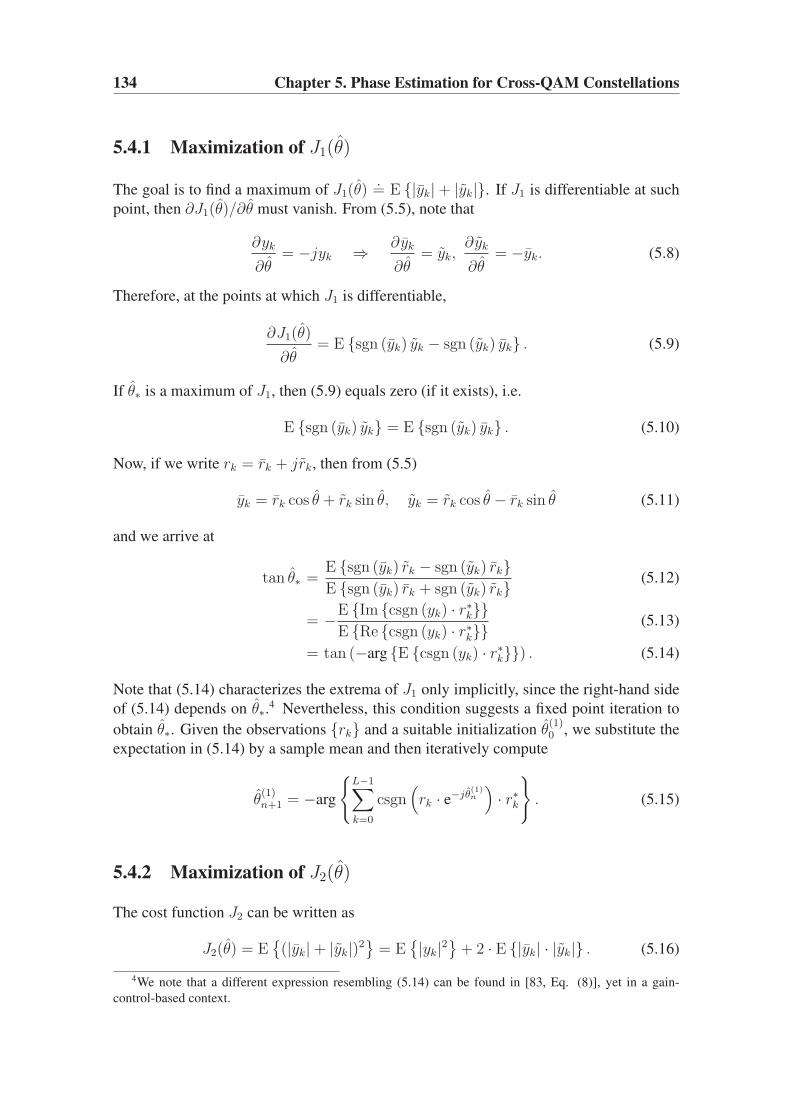
134 Chapter 5. Phase Estimation for Cross-QAM Constellations
5.4.1 Maximization of J1(θ)
The goal is to find a maximum of J1(θ).= E {|yk|+ |yk|}. If J1 is differentiable at such
point, then ∂J1(θ)/∂θ must vanish. From (5.5), note that
∂yk
∂θ= −jyk ⇒ ∂yk
∂θ= yk,
∂ yk
∂θ= −yk. (5.8)
Therefore, at the points at which J1 is differentiable,
∂J1(θ)
∂θ= E {sgn (yk) yk − sgn (yk) yk} . (5.9)
If θ∗ is a maximum of J1, then (5.9) equals zero (if it exists), i.e.
E {sgn (yk) yk} = E {sgn (yk) yk} . (5.10)
Now, if we write rk = rk + jrk, then from (5.5)
yk = rk cos θ + rk sin θ, yk = rk cos θ − rk sin θ (5.11)
and we arrive at
tan θ∗ =E {sgn (yk) rk − sgn (yk) rk}E {sgn (yk) rk + sgn (yk) rk}
(5.12)
= −E {Im {csgn (yk) · r∗k}}E {Re {csgn (yk) · r∗k}}
(5.13)
= tan (−arg {E {csgn (yk) · r∗k}}) . (5.14)
Note that (5.14) characterizes the extrema of J1 only implicitly, since the right-hand side
of (5.14) depends on θ∗.4 Nevertheless, this condition suggests a fixed point iteration to
obtain θ∗. Given the observations {rk} and a suitable initialization θ(1)0 , we substitute the
expectation in (5.14) by a sample mean and then iteratively compute
θ(1)n+1 = −arg
{L−1∑
k=0
csgn(
rk · e−jθ(1)n
)
· r∗k
}
. (5.15)
5.4.2 Maximization of J2(θ)
The cost function J2 can be written as
J2(θ) = E{(|yk|+ |yk|)2
}= E
{|yk|2
}+ 2 · E {|yk| · |yk|} . (5.16)
4We note that a different expression resembling (5.14) can be found in [83, Eq. (8)], yet in a gain-
control-based context.
5.5. Discussion and Statistical Analysis 135
Since E {|yk|2} is invariant under phase rotations, maximizing J2(θ) amounts to maxi-
mizing E {|ykyk|}. Using basic trigonometric relations, it is found that
ykyk = rkrk cos(2θ)−1
2(r2k − r2k) sin(2θ). (5.17)
Therefore, at the points at which J2 is differentiable,
∂J2(θ)
∂θ= −E
{sgn (ykyk) (r2k − r2k)
}cos(2θ)
− E {sgn (ykyk) 2rkrk} sin(2θ). (5.18)
Observe that
r2k − r2k = Re{r2k}, 2rkrk = Im
{r2k}, (5.19)
sk(θ).= sgn (ykyk) = sgn
(
Im{
r2ke−j2θ})
. (5.20)
If θ∗ is a maximum of J2 at which J2 happens to be differentiable, then (5.18) must be
zero, i.e.,
tan(2θ∗) = −E{
Re {r2k} sk(θ∗)}
E{
Im {r2k} sk(θ∗)} (5.21)
= tan(
arg{
−jE{
r2k sk(θ∗)}})
. (5.22)
Since the right-hand side of (5.22) depends on θ∗, this condition does not provide the
desired solution in closed form, but similarly to (5.15), it suggests a fixed point iteration.
Given the observations {rk} and a suitable initialization θ(2)0 , the expectation in (5.22) is
replaced by a sample mean and then θ(2)n is iteratively computed as follows:
sk(θ(2)n ) = sgn
(
Im{
r2ke−j2θ(2)n
})
, k = 0, . . . , L− 1 (5.23a)
θ(2)n+1 =
1
2arg
{L−1∑
k=0
[
r2ksk(θ(2)n )]}
− π
4. (5.23b)
5.5 Discussion and Statistical Analysis
5.5.1 Algorithm Initialization
The cost functions Jq(θ) are multimodal in general, due to finite sample effects; in the
case of cross-QAM, multimodality holds even as L → ∞, see Figure 5.5. Hence the
proposed iterative schemes may experience convergence to undesirable solutions. Initial-
ization must be good enough to set the starting point within the domain of attraction of
the global maximum. Potential initializers include those methods discussed in Section 5.2.
The use of the novel iterative methods as refinements of the standard estimators of Sec-
tion 5.2 is justified only if they are able to provide better performance than the initializer,
and at a reasonable computational cost. Both issues are discussed next.
136 Chapter 5. Phase Estimation for Cross-QAM Constellations
5.5.2 Computational Complexity
Consider the standard 4P estimator (5.3). Obtaining the averaged value∑
k r4k requires
5L real multiplications and 4L real additions [31]. On the other hand, computation of the
C8 estimate (5.4) requires 11L real multiplications and 8L real additions. Thus, the C8
estimate is about twice as expensive as the standard fourth-phase estimate.
However, quantifying the computational load associated to a given estimator is not
always such a straightforward task. Consider for instance the estimate θVV-0 from (5.2),
which must compute∑
k ej4arg{rk} = (∑
k cos(4arg {rk}) + j∑
k sin(4arg {rk}). This
in turn requires (i) extraction of the phase of the complex numbers rk, i.e., Cartesian-to-
Polar (C2P) conversion; (ii) computation of the terms cos(4arg {rk}) and sin(4arg {rk});and (iii) averaging these values. The last step amounts to 2L real additions; however,
the first two steps are likely to be implemented as look-up table (LUT) operations. Thus,
complexity comparisons of the 4P, C8, and V&V-0 estimators will depend on the relative
costs assigned to memory area, hardware multipliers, etc.5
In a similar vein, iteration (5.15) requires L phase rotations (in order to compute
csgn (rk · e−jθ(1)n )) and 2L real additions per iteration. Phase rotations can be performed
very efficiently (with shift-and-add operations only) with CORDIC hardware [85, 114].
Alternatively, with a previous C2P module providing |rk| and arg {rk}, determination of
the csgn terms only requires L additions per iteration. The scheme (5.23) is slightly more
costly than (5.15) due to the need to precompute r2k, although it can also benefit from
C2P/CORDIC modules for the computation of sk(θ(2)n ). Complexity evaluation of the
proposed estimators should also take into account the need for proper initialization, as
well as the fact that some of the partial results of the initialization stage can be reused in
subsequent iterations.
5.5.3 Asymptotic Variances
Using a small-error analysis, it is possible to obtain closed-form expressions for the
asymptotic variances of the estimates θ(q).= limn→∞ θ
(q)n , q = 1, 2. Details are given
in Appendix 5.B, and the results are summarized in the following theorem.
Theorem 1. Assuming that the iterations (5.15) and (5.23) are initialized sufficiently close
to the true phase offset θ and that the signal-to-noise ratio ρ.= Ea/σ
2 is sufficiently high,
the estimates θ(1) and θ(2) are asymptotically unbiased, and their asymptotic variances
are given by
limL→∞
L E{
(θ(1) − θ)2}
=1
2d21
(
(2− d2) +2
ρ
)
(5.24)
limL→∞
L E{
(θ(2) − θ)2}
=1
4g22
(c4 + b4
2+
2
ρ+
1
ρ2
)
(5.25)
5Note that the operation counts given above for the 4P and C8 schemes will change if a previous LUT-
based C2P stage is applied to the observed data, which makes direct comparison with V&V-0 even more
difficult.

5.6. Simulation Results 137
Table 5.1: Asymptotic variance ratios (5.26) for several QAM constellation sizes.
Square QAMs Cross-QAMs
M 16 64 256 1024 32 128 512 2048
α1 2.01 0.93 0.81 0.79 0.06 0.06 0.05 0.05
α2 2.01 0.98 0.86 0.84 0.09 0.08 0.08 0.08
where b4, c4, g2, dn (n = 1, 2) are constellation-dependent constants:
b4.=
E {a4k}E2
a
c4.=
E {|ak|4}E2
a
g2.=
E {a2k sgn (Im {a2k})}Ea
dn.=
E {(a∗k csgn (ak))n}E
n/2a
n = 1, 2.
The asymptotic variances (5.24)-(5.25) depend on the constellation and the SNR, but
not on the value of θ; this is also the case for the 4P estimate, whose asymptotic variance
is given in [30, 142]. Using that expression and (5.24)-(5.25), one can obtain the ratio of
limits (as the SNR tends to infinity) of the asymptotic variances of the new estimates to
that of the 4P estimate
αq.=
limρ,L→∞ L E{
(θ(q) − θ)2}
limρ,L→∞ L E{
(θ4P − θ)2} . (5.26)
These ratios are given in Table 5.1, showing that the new schemes perform similarly to
the 4P estimator with square QAM, but they consistently offer a sizable improvement
(about one order of magnitude reduction of the asymptotic variance) with cross-QAM
constellations.
5.6 Simulation Results
We present the results obtained with the novel iterative estimators, using Monte Carlo
simulations, under both floating point and fixed point implementations. The focus is on
32-QAM and 128-QAM cross constellations. Results are presented in terms of bias and
Root Mean Square Error (RMSE), defined as
RMSE.=
√
E
{
min
{(
θ − θ)2
,(
θ − θ +π
2
)2
,(
θ − θ − π
2
)2}}
where the min{·} function represents the fact that a practical receiver should be able to
remove the π/2-ambiguity of the QAM phase estimator. Bias and RMSE are estimated
via the Monte Carlo method.
138 Chapter 5. Phase Estimation for Cross-QAM Constellations
5.6.1 Floating Point Precision
Convergence properties were investigated first, with a phase offset θ = 20◦. Figure 5.6
shows the RMSE as a function of the number of iterations. Both estimators were initial-
ized using the 4P method (the RMSE shown for iteration zero corresponds to θ4P), and
different values of the SNR per bit [defined as Eb/N0.= Ea/(σ
2 log2M)] are consid-
ered. Convergence slows down with decreasing Eb/N0 as expected, but nevertheless, for
practical situations a few iterations suffice.
0 2 4 6 8 100.5
1
1.5
2
2.5
3
3.5
iterations
RM
SE
(deg
)
32-QAM, θ = 20◦, L = 1024
J1(4P)J2(4P)
Eb/N0 = 10 dB
Eb/N0 = 20 dB
(a)
0 2 4 6 8 101
1.25
1.5
1.75
2
2.25
2.5
iterations
RM
SE
(deg
)
128-QAM, θ = 20◦, L = 2048
J1(4P)J2(4P)
Eb/N0 = 15 dB
Eb/N0 = 30 dB
(b)
Figure 5.6: RMSE versus number of iterations for (a) 32-QAM and (b) 128-QAM. The
method in parentheses after J1 and J2 indicates which estimator was used as initializer for
the respective iteration.
Note from Figure 5.6 that for 128-QAM and Eb/N0 = 30 dB, the RMSE actually
increases after the second iteration. This effect is due to the fact that, occasionally, the
initializer (θ4P in this case) will fail to set the starting point within the domain of attraction
of the desired solution, so that convergence to an undesired local maximum of the cost
function Jq takes place. The nonzero probability of these events introduces a bias in the
estimates, which in turn pulls up the final RMSE.
Figure 5.7 shows the RMSE of the proposed estimators (fixing the number of itera-
tions to five), together with those of θ4P and θC8, as a function of the SNR per bit. For
32-QAM, the iterative estimators are initialized at θ4P; they perform similarly to θC8 in
the high Eb/N0 region, although θC8 degrades more gracefully as the noise increases.
Good agreement with the theoretical variance predicted by (5.24)-(5.25) is observed for
Eb/N0 ≥ 14 dB.
Whereas θ4P seems to be a sufficiently good initializer with 32-QAM, the situation is
different for 128-QAM: occasional convergence to local maxima prevents the RMSE of
the iterative estimators from reaching their theoretical asymptotic values. Another option
is to use θC8 as initializer. Note from Figure 5.7 that the theoretical RMSE of the iterative
estimators with 128-QAM in high SNR lies below the observed RMSE of θC8, so that

5.6. Simulation Results 139
10 15 20 25 300.5
1
1.5
2
2.5
3
3.5
4
Eb/N0 (dB)
RM
SE
(deg
)
32-QAM, θ = 20◦, L = 1024
(a)
10 15 20 25 300.5
1
1.5
2
2.5
3
Eb/N0 (dB)
RM
SE
(deg
)
128-QAM, θ = 20◦, L = 2048
(b)
Figure 5.7: RMSE versus SNR per bit for (a) 32-QAM and (b) 128-QAM. Markers are as
follows: 4P (�), C8 (♦), J1 (×), J2 (◦). J1 and J2 are initialized with 4P (solid line) and
C8 (dashed line). Dashed thin lines indicate the theoretical RMSE values for estimators
θ4P, θ(1) and θ(2).
it makes sense to apply these schemes as refinements to θC8. As shown, this initializer
avoids the problem of convergence to local maxima.
This same trend can be observed in Figure 5.8, which displays the SER achieved
after application of the proposed estimators in comparison with the one-shot estimates
(4P and C8) which serve as intializers. Considering the 32-QAM, the poor performance
of 4P as initializer poses difficulties to the iterative methods, whose SER degrades above
Eb/N0 = 16 dB due to the convergence to local maxima. However, 4P seems a good
initializer below Eb/N0 = 14 dB (i.e., for SER ≤ 10−3). Initialization with a better
estimate (C8) allows both J1 and J2 to stay close to reference SER with no phase offset.
This is more clearly seen in the case of the 128-QAM, where the improvement of the
iterative schemes over the initializers is evident. It is noticeable that J1 and J2 are able to
significantly reduce the Eb/N0 penalty of the best initializer at high SNRs (C8).
Of course, all these considerations depend on the number of samples L used for the
estimation; too low a value of L could result in θC8 not being a good initializer either.
But in general, it can be said that the novel estimators have the potential to improve
the performance of either fourth-order or eighth-order schemes with low computational
complexity. This potential is even greater under finite precision constraints, as discussed
next.
5.6.2 Fixed Point Implementation
The performance of the different estimators is evaluated under quantization and fixed
point arithmetic conditions. The goal is to test the robustness of each method under real-
istic implementation constraints. The receiver ADC quantizes each real-valued (in-phase
and quadrature) data sample to B bits. The binary point is set to the right of the first bit,

140 Chapter 5. Phase Estimation for Cross-QAM Constellations
6 8 10 12 14 16 18 2010
−6
10−5
10−4
10−3
10−2
10−1
100
SE
R
Eb/N0 (dB)
32-QAM
AWGN, no offset
4P
C8
J1(4P)
J1(C8)
J2(4P)
J2(C8)
(a)
10 12 14 16 18 20 22 24 26
10−4
10−3
10−2
10−1
100
SE
R
Eb/N0 (dB)
128-QAM
AWGN, no offset
4P
C8
J1(4P)
J1(C8)
J2(4P)
J2(C8)
(b)
Figure 5.8: SER versus Eb/N0 after phase correction for (a) 32-QAM, L = 1024 samples,
and (b) 128-QAM, L = 2048 samples, both with θ = 20◦. The thin dashed line indicates
the SER under no phase offset.
which is the sign bit. The full-scale value of the ADC (i.e., the maximum representable
amplitude) is chosen in order to set the probability of clipping at 10−3 under AWGN,
measured at a reference SNR for which a raw SER of 10−1 is obtained.6
When working with fixed point systems, care must be taken in order to minimize the
effects of underflow and overflow. Appropriate scalings must be introduced at certain
stages in order to obtain a suitable tradeoff between the probabilities of these two undesir-
able events, denoted by Pu and Po respectively. The locations and values (usually powers
of two, for efficiency reasons) of the scaling factors must be determined by careful study
of Pu and Po at each of the intermediate computations. Of the estimators considered in
this chapter, it was found that scaling was beneficial for the C8 and 4P schemes when
B ≤ 18 and 9 bits respectively, but not for the proposed iterative methods. This confirms
what one would expect by considering the number of products involved in each case.
In the simulations, wordlengths ranging from B = 30 down to 8 bits have been tested,
and the scalings were optimized for each estimator. When B is sufficiently high, the
convergence and the RMSE of all estimators follow the floating point results shown in
the previous section. However, the performance of the methods tested degrades below a
certain value of B, which depends on the estimator and the constellation. It was observed
that in general θC8 is more sensitive to finite wordlength effects than the rest of estimators,
whereas θ(1) and θ(2) are much more robust in this sense. Next we review in detail the
results of our fixed point simulations in terms of bias and RMSE for the 32-QAM and
128-QAM constellations.
6The probability of clipping is the probability that the noisy received in-phase or quadrature components
exceed the full-scale value. Since this probability depends on the noise variance, some reference noise
variance must be considered. Such noise variance is provided by the SNR point for which the uncoded SER
of the constellation equals 10−1.

5.6. Simulation Results 141
5.6.2.1 Fixed Point Bias
−40 −30 −20 −10 0 10 20 30 40−1.5
−1
−0.5
0
0.5
1
1.5
Phase offset θ (deg)
Bia
s(d
eg)
(a) 32-QAM, L = 1024, Eb/N0 = 30 dB, 14 bits
4PC8J1(4P)J2(4P)
−40 −30 −20 −10 0 10 20 30 40−1.5
−1
−0.5
0
0.5
1
1.5
Phase offset θ (deg)
Bia
s(d
eg)
(b) 32-QAM, L = 1024, Eb/N0 = 30 dB, 12 bits
−40 −30 −20 −10 0 10 20 30 40−1.5
−1
−0.5
0
0.5
1
1.5
Phase offset θ (deg)
Bia
s(d
eg)
(c) 32-QAM, L = 1024, Eb/N0 = 30 dB, 10 bits
−40 −20 0 20 40−50
−25
0
25
50
−40 −30 −20 −10 0 10 20 30 40−5
−4
−3
−2
−1
0
1
2
3
4
5
Phase offset θ (deg)
Bia
s(d
eg)
(d) 32-QAM, L = 1024, Eb/N0 = 30 dB, 8 bits
−40 −20 0 20 40−50
−25
0
25
50
Figure 5.9: Bias versus θ. 32-QAM, L = 1024, Eb/N0 = 30 dB. (a) B = 14, (b) B = 12,
(c) B = 10, and (d) B = 8 bits. Markers are common to all figures as indicated in (a).
All estimators are unbiased for sufficiently large wordlengths, but as B is decreased
an offset-dependent bias appears, whose magnitude grows inversely to B. Figures 5.9
and 5.10 show the bias for 32-QAM and 128-QAM respectively in terms of θ, at Eb/N0 =30 dB and for different wordlengths. At such high SNR values, the bias can only be
attributable to finite precision effects. Clearly, θC8 is more severely affected than the rest
of estimators. For 32-QAM, θC8 already shows bias at B = 14 bits, and for B ≤ 10 bits
it becomes useless. The remaining estimators degrade more gracefully, with θ4P and θ(2)
exhibiting the smallest peak bias (about 0.3◦ and 1.0◦ for B = 10 and 8 bits respectively).
For 128-QAM, θC8 is seen to have a large peak bias of 2◦ already for B = 14 bits. The
bias of the other schemes becomes noticeable only for B ≤ 12 bits.
5.6.2.2 Fixed Point RMSE
Results for 32-QAM are given in Figure 5.11(a)–(c) for L = 1024 symbols, θ = 20◦ and
different values of B. With B > 12 bits, all methods perform similarly to the floating
point case. For B = 12 bits, only θC8 shows a small degradation, which becomes very
large for smaller wordlengths. In contrast, θ4P is not as sensitive, similarly to the novel
estimators θ(1), θ(2), which achieve a much smaller asymptotic RMSE. We note that the
small decrease in RMSE with respect to the finite precision curve is achieved in exchange
for a slight bias.

142 Chapter 5. Phase Estimation for Cross-QAM Constellations
−40 −30 −20 −10 0 10 20 30 40−3
−2
−1
0
1
2
3
Phase offset θ (deg)
Bia
s(d
eg)
(a) 128-QAM, L = 2048, Eb/N0 = 30 dB, 14 bits
−40 −30 −20 −10 0 10 20 30 40−3
−2
−1
0
1
2
3
Phase offset θ (deg)
Bia
s(d
eg)
(b) 128-QAM, L = 2048, Eb/N0 = 30 dB, 12 bits
−40 −30 −20 −10 0 10 20 30 40−6
−4
−2
0
2
4
6
Phase offset θ (deg)
Bia
s(d
eg)
(c) 128-QAM, L = 2048, Eb/N0 = 30 dB, 10 bits
−40 −30 −20 −10 0 10 20 30 40
−30
−20
−10
0
10
20
30
Phase offset θ (deg)
Bia
s(d
eg)
(d) 128-QAM, L = 2048, Eb/N0 = 30 dB, 8 bits
4PC8J1(4P)J2(4P)
Figure 5.10: Bias versus θ. 128-QAM, L = 2048, Eb/N0 = 30 dB. (a) B = 14, (b)
B = 12, (c) B = 10, and (d) B = 8 bits. Markers are common to all figures as indicated
in (d).
Results for 128-QAM, see Figure 5.11(d)–(f), roughly follow those for 32-QAM, but
with all estimators suffering larger performance losses. For B = 14 and 12 bits, θC8
exhibits a large RMSE of about 2◦ (due to its large bias, see Figure 5.10). Nevertheless, it
still provides a good initializer for θ(1) and θ(2), which reach their asymptotic variances at
high Eb/N0. For B = 10 the high RMSE of θC8 (3.3◦) pulls up the RMSEs of θ(1) and θ(2)
when they start from θC8. The performance of θ4P is not affected by finite wordlengths as
small as B = 10 bits, and thus when this estimate is used to initialize θ(1) and θ(2), these
achieve the same RMSE as in the floating point implementation (see Figure 5.7b).
To wrap up, the two proposed phase estimators present advantages over existing higher-
order methods in terms of finite precision implementation. Whereas the higher-order met-
gods are clearly seen to suffer from finite precision issues, the proposed estimators are
able to hold their good performance under tight wordlength constraints thanks to their
lower statistical order. This makes them appealing choices for practical receiver design
under e.g. fixed point implementation. Regarding their initialization, we have seen that
standard one-shot methods can provide adequate coarse estimators for this purpose, upon
which the proposed methods are able to provide refined estimates.
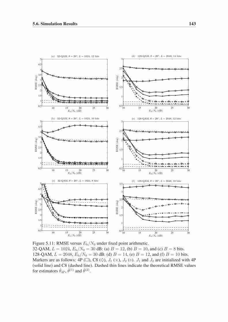
5.6. Simulation Results 143
10 15 20 25 300.5
1
1.5
2
2.5
3
3.5
4
4.5
5
Eb/N0 (dB)
RM
SE
(deg
)
(a) 32-QAM, θ = 20◦, L = 1024, 12 bits
10 15 20 25 300.5
1
1.5
2
2.5
3
3.5
4
4.5
5
Eb/N0 (dB)
RM
SE
(deg
)
(b) 32-QAM, θ = 20◦, L = 1024, 10 bits
10 15 20 25 300.5
1
1.5
2
2.5
3
3.5
4
4.5
5
Eb/N0 (dB)
RM
SE
(deg
)
(c) 32-QAM, θ = 20◦, L = 1024, 8 bits
10 15 20 25 300.5
1
1.5
2
2.5
3
Eb/N0 (dB)
RM
SE
(deg
)
(d) 128-QAM, θ = 20◦, L = 2048, 14 bits
10 15 20 25 300.5
1
1.5
2
2.5
3
Eb/N0 (dB)
RM
SE
(deg
)(e) 128-QAM, θ = 20◦, L = 2048, 12 bits
10 15 20 25 300.5
1
1.5
2
2.5
3
3.5
Eb/N0 (dB)
RM
SE
(deg
)
(f ) 128-QAM, θ = 20◦, L = 2048, 10 bits
Figure 5.11: RMSE versus Eb/N0 under fixed point arithmetic.
32-QAM, L = 1024, Eb/N0 = 30 dB: (a) B = 12, (b) B = 10, and (c) B = 8 bits.
128-QAM, L = 2048, Eb/N0 = 30 dB: (d) B = 14, (e) B = 12, and (f) B = 10 bits.
Markers are as follows: 4P (�), C8 (♦), J1 (×), J2 (◦). J1 and J2 are initialized with 4P
(solid line) and C8 (dashed line). Dashed thin lines indicate the theoretical RMSE values
for estimators θ4P, θ(1) and θ(2).
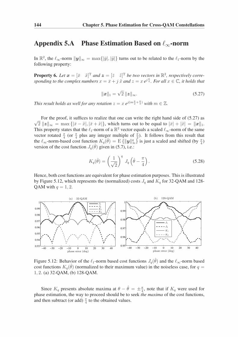
144 Chapter 5. Phase Estimation for Cross-QAM Constellations
Appendix 5.A Phase Estimation Based on ℓ∞-norm
In R2, the ℓ∞-norm ‖y‖∞ = max{|y|, |y|} turns out to be related to the ℓ1-norm by the
following property:
Property 6. Let x = [x x]T and z = [z z]T be two vectors in R2, respectively corre-
sponding to the complex numbers x = x+ j x and z = x ejπ4 . For all x ∈ C, it holds that
‖x‖1 =√2 ‖z‖∞. (5.27)
This result holds as well for any rotation z = x ej(mπ2+π
4) with m ∈ Z.
For the proof, it suffices to realize that one can write the right hand side of (5.27) as√2 ‖z‖∞ = max {|x− x|, |x+ x|}, which turns out to be equal to |x| + |x| = ‖x‖1.
This property states that the ℓ1-norm of a R2 vector equals a scaled ℓ∞-norm of the same
vector rotated π4
(or π4
plus any integer multiple of π2). It follows from this result that
the ℓ∞-norm-based cost function Kq(θ) = E {‖y‖q∞} is just a scaled and shifted (by π4)
version of the cost function Jq(θ) given in (5.7), i.e.:
Kq(θ) =
(1√2
)q
Jq
(
θ − π
4
)
. (5.28)
Hence, both cost functions are equivalent for phase estimation purposes. This is illustrated
by Figure 5.12, which represents the (normalized) costs Jq and Kq for 32-QAM and 128-
QAM with q = 1, 2.
−40 −30 −20 −10 0 10 20 30 400.93
0.94
0.95
0.96
0.97
0.98
0.99
1
phase error (deg)
(a) 32-QAM
J1
J2
K1
K2
−40 −30 −20 −10 0 10 20 30 400.95
0.96
0.97
0.98
0.99
1
phase error (deg)
(b) 128-QAM
J1
J2
K1
K2
Figure 5.12: Behavior of the ℓ1-norm based cost functions Jq(θ) and the ℓ∞-norm based
cost functions Kq(θ) (normalized to their maximum value) in the noiseless case, for q =1, 2. (a) 32-QAM, (b) 128-QAM.
Since Kq presents absolute maxima at θ − θ = ±π4, note that if Kq were used for
phase estimation, the way to proceed should be to seek the maxima of the cost functions,
and then subtract (or add) π4
to the obtained values.

5.B. Proof of Theorem 1 145
Appendix 5.B Proof of Theorem 1
We will prove (5.24), as the proof of (5.25) follows completely analogous steps. Let θ(1)
be a fixed point of (5.15). In order to prove (5.24), let us define
η.=
1
L
L−1∑
k=0
r∗k csgn(
rk e−jθ(1))
. (5.29)
Then θ(1) satisfies θ(1) = −arg {η}. Let us also define
η.= E
{r∗k csgn
(rk e−jθ
)}= η + jη (5.30)
where θ is the true phase offset. Then, similarly to [142], we can write
θ(1) = −tan−1
(Im {η}Re {η}
)
= −tan−1
(Im {η} − Im {η − η}Re {η} − Re {η − η}
)
(5.31)
so that a first-order approximation of the argument in (5.31) yields
θ(1) ≈ −tan−1
(η
η+ ǫ
)
(5.32)
ǫ.=
1
η
(
Im {η − η} − η
ηRe {η − η}
)
. (5.33)
Note that rk e−jθ = ak + mk, where mk = nk e−jθ is a noise process with the same
statistical properties as nk. Hence, if the SNR is sufficiently high, then
csgn(rk e−jθ
)= csgn (ak +mk) ≈ csgn (ak)
so that
η ≈ E {r∗k csgn (ak)} (5.34)
= E {a∗k csgn (ak)}︸ ︷︷ ︸
=√Ea d1
e−jθ + E {n∗k csgn (ak)}
︸ ︷︷ ︸
=0
(5.35)
and the approximation error in (5.34) decays exponentially fast with the SNR. The statistic
d1 (defined in Theorem 1) turns out to be real and positive for QAM constellations, and
therefore −tan−1(η/η) → θ as the SNR goes to infinity. Then a first-order expansion
of (5.32) yields
θ(1) ≈ θ − ǫ · cos2 θ. (5.36)
With the asymptotic approximation η ≈√Ea d1 e−jθ, (5.33) becomes
ǫ ≈ Im{(η − η) ejθ
}/(η cos θ). (5.37)
146 Chapter 5. Phase Estimation for Cross-QAM Constellations
Note that if the SNR is sufficiently large and the phase error θ − θ(1) is sufficiently small,
then η is an unbiased estimate of η:
E {η} =1
L
L−1∑
k=0
E{
r∗k csgn(
rk e−jθ(1))}
=1
L
L−1∑
k=0
E{
r∗k csgn(
ak ej(θ−θ(1)) + nk e−jθ(1))}
≈ 1
L
L−1∑
k=0
E {r∗k csgn (ak)} ≈ η. (5.38)
Hence, from (5.36)-(5.38), θ(1) is asymptotically unbiased.
In order to compute the asymptotic variance, some straightforward manipulations
show that
Im2{(η − η) ejθ
}=
1
2
[|η − η|2 − Re
{(η − η)2 ej2θ
}]. (5.39)
Therefore, from (5.36)-(5.37) and (5.39),
limL→∞
L E{
(θ(1) − θ)2}
= cos4 θ limL→∞
L E{ǫ2}
(5.40)
=cos2 θ
2η2limL→∞
L[E{|η − η|2
}− Re
{E{(η − η)2
}ej2θ}]
(5.41)
where the expectations in (5.41) are given by
E{|η − η|2
}= E
{|η|2 − |η|2
}
≈ 1
L2
L−1∑
k=0
L−1∑
l=0
E{r∗k rl csgn
(rk e−jθ
)csgn∗ (rl e−jθ
)}− |η|2 (5.42)
=(L2 − L)
L2
∣∣E{r∗k csgn
(rk e−jθ
)}∣∣2
+1
L2
L−1∑
k=0
E{
|rk|2∣∣csgn
(rk e−jθ
)∣∣2}
− |η|2 (5.43)
=
(
1− 1
L
)
|η|2 + 2
LE{|rk|2
}− |η|2 (5.44)
=1
L
(2Ea + 2σ2 − |η|2
)(5.45)

5.B. Proof of Theorem 1 147
E{(η − η)2
}= E
{η2 − η2
}
≈ 1
L2
L−1∑
k=0
L−1∑
l=0
E{r∗k r
∗l csgn
(rk e−jθ
)csgn
(rl e−jθ
)}− η2 (5.46)
=(L2 − L)
L2E2{r∗k csgn
(rk e−jθ
)}
+1
L2
L−1∑
k=0
E{(
r∗k csgn(rk e−jθ
))2}
− η2 (5.47)
≈(
1− 1
L
)
η2 +1
LE{(r∗k csgn (ak))
2}− η2 (5.48)
=1
L
(Ea d2 e−j2θ − η2
). (5.49)
Note that d2 is defined in Theorem 1. Now, substituting (5.45) and (5.49) in (5.41), and
noting that η2 = Ea d21 cos2 θ, the final result (5.24) is obtained.


Chapter 6Conclusions and Future Lines
Contents
6.1 Conclusions . . . . . . . . . . . . . . . . . . . . . . . . . . . . . . . . 149
6.2 Future Research Lines . . . . . . . . . . . . . . . . . . . . . . . . . . 151
6.1 Conclusions
We proposed the joint use of shaping without scrambling (i.e., the combination of Tomlinson-
Harashima Precoding (THP) and signal shaping) and signal predistortion in the context
of a downlink point-to-point satellite service making use of gap fillers to complete the
satellite coverage. The signals coming from the gap fillers introduce diversity in the re-
ceived signal, which, unless properly processed, translates into undesired Intersymbol
Interference (ISI). We saw that the combination of shaping without scrambling and signal
predistortion successfully counteracts the gap filler-induced ISI and the nonlinear dis-
tortion caused by the High Power Amplifier onboard the satellite. The role of shaping
without scrambling is to modify the shape of the precoded signal so that the HPA-induced
distortion is minimum. With this goal, different shaping metrics have been tested with
similar net results in terms of BER. All in all, the proposed scheme may constitute an
attractive solution for practical systems with fixed and nomadic terminals, since the ISI is
precanceled at the transmitter (e.g., the gateway), which should simplify the complexity
of the terminals.
THP was also considered for the downlink of a satellite multibeam satellite system
providing independent data streams to each beam. The THP operation, which is to be
preferably performed at the gateway, was used to cancel the Co-Channel Interference
(CCI) that each terminal receives from the neighboring beams reusing the same frequency.
Several application scenarios were tested, based on a realistic beam pattern, and for sev-
eral terminal locations and frequency reuse factors. We saw that the adoption of THP
in this context can achieve the proper removal of the unwanted CCI. This, in turn, may

150 Chapter 6. Conclusions and Future Lines
reduce the frequency reuse factor required in current multibeam systems to prevent an
excess of CCI, especially when a single centralized gateway performs the precoding for
a large number of beams. The application of Linear Precoding (LP) to similar scenarios
was analyzed in detail in [43, 67] offering interesting potential improvements in terms of
throughput with respect to traditional systems. Our work shows that even greater improve-
ments can be expected if THP is used, mainly due to the removal of the transmit power
penalty inherent to LP schemes. This fact has attracted the interest of recent surveys
devoted to identify novel transmission technologies for future satellite systems, e.g. [15].
In what regards the problem of Signal-to-Noise Ratio (SNR) estimation, we saw that
the use of higher-order moments is an interesting approach for estimator design, particu-
larly considering the SNR estimation from higher modulations such as the two- and three-
level APSK constellations used in the DVB-S2 standard. We developed an SNR estimator
based on eighth-order statistics, which can be efficiently implemented without look-up
tables. The estimator is built upon a linear combination of ratios of moments, whose
weights can be tuned according to the constellation and the SNR operation range. Two
weight optimization criteria were proposed, which yield good estimators with improved
performance over existing methods. The new higher-order approach, which generalizes
many of the previous moments-based estimators existing in the literature, can be easily
extended to any statistical order and to any modulation order. The analysis and optimiza-
tion of such extensions can be carried out using the same approach and tools that were
applied to the eighth-order estimator.
We also studied the problem of estimating the SNR from heterogeneous frames, i.e.,
frames containing two (or more) subframes, each one formed by symbols drawn from
a different constellation. Such kind of frames are commonly found in current systems
in which the data-bearing symbols can belong to higher modulations, whereas simpler
modulations are chosen for the header and the pilot symbols. The DVB-S2 standard
provides a practical case of application of our approach. By exploiting the knowledge
of the symbol set we obtained the CRB for the problem and we proposed a number of
possible heterogeneous estimators of which the so called convex combination of estimates
(CCE) proved to be the best choice. Analysis of the MSEs of the proposed estimators
showed that the CCE estimator outperforms the constituent estimators, and also the rest of
the heterogeneous estimators considered. Furthermore, CCE estimators are rather flexible
since they can combine any type of constituent estimators, including data-aided ones. We
have seen that this last feature is a further advantage of the CCE scheme when training
symbols (pilots, partially known header) are available in the heterogeneous frame.
As for the problem of phase estimation, we introduced two iterative low-order phase
estimators for cross-QAM constellations (e.g. 32-QAM, 128-QAM) whose performance
achieves that of higher-oder schemes specifically derived for such constellations. The pro-
posed estimators do not require neither gain control nor data knowledge, and feature a low
statistical order, which turns into an advantage when they are to be implemented under
finite precision conditions. Whereas higher-order methods are clearly seen to suffer from
finite precision issues, the proposed estimators are able to hold their good performance
under tight wordlength constraints, which makes them appealing choices for practical
receiver design under e.g. fixed point implementation. A key issue in the proposed it-

6.2. Future Research Lines 151
erative estimators is their initialization. We saw that standard one-shot methods (eighth-
and fourth-order) can provide adequate coarse estimators for this purpose, upon which
the proposed methods are able to provide refined estimates. Different initialization strate-
gies are also possible: for example, the low complexity of the Viterbi&Viterbi estimators
of 0-th and negative orders makes them attractive initializers at low and high SNRs, re-
spectively. Yet another possibility arises whenever training symbols are inserted in the
transmitted frame, as it is usually the case in practice. A data-aided phase estimator based
just on these training symbols may well present a variance too large for decoding purposes
(due to a limited number of training data), but sufficiently low to initialize the proposed
iterative schemes. Such semiblind approach would significantly improve the quality of
the plain data-aided phase estimate.
6.2 Future Research Lines
The performance analysis of THP developed in Chapters 2 and 3 has been possible thanks
to the adoption of certain simplifying assumptions. The list of assumptions for each chap-
ter can be found in pages 23 and 63. Among these assumptions, the most demanding
ones are probably the following: perfect timing and carrier recovery, perfect CSI knowl-
edge at the transmitter, and linear HPAs. The two former assumptions are common to
the proposed SISO and multibeam systems, whereas the latter was used in the multibeam
case only. In Appendices 2.B, 3.E, and 3.D we have provided an overview of these is-
sues, as well as some of the approaches available in the open literature. A completely
realistic system analysis would require to evaluate the impact in performance of practical
timing and carrier recovery schemes, practical CSI retrieval schemes, and practical HPA
linearization schemes (e.g. predistortion). Furthermore, no coding was considered in the
THP systems analyzed in Chapters 2 and 3. The introduction of coding (e.g. the LDPC
codes considered in 10GBASE-T) would allow a complete system analysis in terms of
throughput.
Under a more fundamental approach, it would be interesting to consider the use of
hexagonal Voronoi regions in the THP operation. In comparison with the squares pro-
vided by the standard modulo operation, the hexagons automatically provide certain shap-
ing gain at the cost of a more complex precoding (and decoding) operation. It would be
also interesting to consider the application of THP to staggered modulation formats such
as offset-QPSK or offset-QAM. Such modulations produce waveforms with reduced en-
velope fluctuations, which would complement the effect of predistortion as a means to
mitigate the impact of the nonlinear HPA. To conclude the THP-related future research
lines, now focusing on the receiver operation, the problem of timing recovery from THP
signals does not yet seem to have received enough interest within the research commu-
nity. In this sense, it seems possible to improve the performance of current NDA timing
recovery schemes when applied to THP signals. This line could be complemented with
the computation of the corresponding CRB for the problem.
Regarding the SNR estimation problem, two topics appear as the natural continuation
of the novel moments-based approach. First, the eighth-order estimator proposed in Sec-

152 Chapter 6. Conclusions and Future Lines
tion 4.3 could be extended to higher orders (e.g. extending the linear combination with
tenth-order statistics), which would presumably bring further performance improvements
thanks to the use of more ratios of moments. Second, the generalized approach to SNR
estimation based on moments of any order, as presented in Appendix 4.B, could be used
to develop novel SNR estimators of low order (e.g., third or fourth) with presumably good
performance for multilevel constellations at intermediate and high SNRs. In addition to
these two lines, another interesting topic of further research is the problem of estimating
the SNR from oversampled data. In this context, several estimators have been recently
proposed [70, 136, 143], although there seems to be room for new estimators as well as
for finding the CRB for the problem.
As for the proposed phase estimation schemes, the potential local convergence issues
caused by the multimodality of the proposed ℓ1-norm-based cost functions makes it desir-
able to find other cost functions suitable for phase estimation avoiding such issues. From
a more general perspective, an interesting problem is the design of joint schemes for SNR
estimation and carrier recovery. Although it has been recently shown that the CRBs for
SNR estimation and carrier recovery (phase and frequency) are decoupled [73], this does
not mean that a suboptimal estimation scheme cannot benefit from a joint approach. In
fact, it turns out that optimal (CRB-achieving) NDA estimation schemes are computa-
tionally intensive, so the seek for suboptimal but simpler estimation schemes would be
justified.

Capıtulo 7Resumen en castellano
Contents
7.1 Aplicacion de THP a la transmision punto a punto por satelite . . . 154
7.2 Aplicacion de THP en sistemas de transmision multihaz por satelite 159
7.3 Estimacion de SNR . . . . . . . . . . . . . . . . . . . . . . . . . . . 163
7.4 Estimacion de fase para modulaciones QAM en cruz . . . . . . . . . 169
Desde el inicio de las telecomunicaciones, la evolucion hacia sistemas de transmision
de mayor capacidad y eficiencia ha sido una constante. Generalmente, la aparicion de una
nueva tecnologıa de transmision o de una tecnica de procesado de senal suscita la creacion
de nuevas aplicaciones en las que estas tecnicas resultan utiles y eficientes. Tras una fase
de investigacion y optimizacion, dichas tecnologıas, ya maduras, acaban aportando una
mayor capacidad de transmision a los sistemas reales en los que se emplean. Sin embar-
go, la demanda eficiencia y capacidad de transmision es siempre creciente, y tan pronto
las nuevas tecnicas son asimiladas y explotadas no tardan en aparecer otras nuevas que
mejoran a sus predecesoras. Como ejemplo, observese la evolucion de las comunicacio-
nes por satelite, en donde en poco mas de 50 anos se ha pasado de la puesta en orbita del
primer satelite artificial (Sputnik-I, 1957) y el primer satelite dedicado a comunicaciones
(TelStar 1, 1962) a planear la puesta en orbita de satelites con una tasa de transferencia
total de 100 Gbps [88].
Esta tesis se centra en gran parte en diversos aspectos relacionados con la capa fısica
de la transmision vıa satelite. Por una parte, los capıtulos 2 y 3 se centran en aspec-
tos relacionados con el transmisor. En particular, se propone la aplicacion de la tecnica
de transmision conocida como precodificacion Tomlinson-Harashima (THP, del ingles
Tomlinson-Harashima precoding) a la transmision por satelite. Ası, en el Capıtulo 2 se
explora la aplicacion de THP en sistemas de transmision punto a punto, mientras que el
Capıtulo 3 se ocupa de la aplicacion a sistemas con cobertura multihaz. Por su parte, los
capıtulos 4 y 5 se centran en la mejora de tecnicas de procesado realizadas en el receptor,
en particular, en metodos estimacion de parametros de senal. En particular, el Capıtulo 4
trata de la estimacion del la relacion senal a ruido (SNR, del ingles signal-to-noise ratio)
154 Capıtulo 7. Resumen en castellano
en el receptor, y tiene una vocacion de aplicacion general, incluyendo las modulaciones
empleadas actualmente en transmision por satelite. El Capıtulo 5 trata de la estimacion de
fase en el receptor para modulaciones QAM en cruz, que son modulaciones en amplitud y
cuadratura (QAM, del ingles quadrature-amplitude modulation) utilizadas exclusivamen-
te en sistemas de comunicaciones terrestres. A continuacion se resumira el contenido de
los cuatro capıtulos principales de esta tesis.
7.1 Aplicacion de THP a la transmision punto a punto
por satelite
En los ultimos anos ha surgido un gran numero de servicios de comunicacion que emplean
un satelite geoestacionario como un medio eficaz para dar cobertura a grandes regiones.
Sin embargo, esa cobertura puede no ser todo lo completa que serıa deseable debido a que
la senal proveniente del satelite no alcanza a todos los posibles receptores. Esto sucede
especialmente en zonas urbanas densamente pobladas, en donde las edificaciones, espe-
cialmente las de gran altura, representan obstaculos insalvables que bloquean completa-
mente la propagacion de la senal del satelite. Ante esta situacion, una de las soluciones es
el empleo de repetidores modulares intermedios (IMRs, del ingles intermediate module
repeaters, tambien conocidos como gap-fillers). Los IMRs actuan como repetidores de
la senal del satelite, y dan cobertura a las zonas a las que no llega la senal del satelite.
Ejemplos del uso de IMRs se pueden encontrar en [12, 48, 55, 84, 105, 109, 130]. El em-
pleo de IMRs es positivo en el sentido de que introduce diversidad en la senal recibida
por los terminales. Sin embargo, esta diversidad viene asociada a una dispersion temporal
en la senal recibida, que se traduce en la existencia de interferencia entre sımbolos (ISI,
del ingles, intersymbol interference). Para una correcta recepcion de la senal deseada, el
receptor debera aplicar algun tipo de medida de compensacion adecuada, como por ejem-
plo combinacion de diversidad, o igualacion de canal, como por ejemplo la igualacion
mediante realimentacion de decisiones (DFE, del ingles decision feedback equalization).
En el Capıtulo 2 de esta tesis se propone el empleo de THP para la compensacion de
la ISI presente en sistemas de transmision punto a punto por satelite que emplean IMRs
en el enlace descendente para completar la cobertura. En [59] se puede encontrar una in-
troduccion muy completa a la transmision THP. La figura 7.1 se muestra el modelo basico
en tiempo discreto de la transmision THP, en donde H(z) es la funcion de transferencia
discreta equivalente del canal, y MOD∆ (·) representa una operacion modulo, por tanto
no lineal. Los sımbolos de entrada, an, que supondremos pertenecientes a constelaciones
QAM cuadradas, son precodificados mediante el lazo indicado en la figura, obteniendo-
se la secuencia precodificada xn = MOD∆
(an −
∑p−1k=1 hk xn−k
). Esta operacion puede
verse como una suerte de igualacion de canal que se realiza en el transmisor, en vez de en
el receptor. Muy similar a la preigualacion lineal de canal, THP introduce una operacion
no lineal en la preigualacion (MOD∆ (·)) que permite evitar el principal inconveniente de
la preigualacion lineal: la penalizacion de potencia transmitida. Ademas, el hecho de que
la operacion se realice en transmision evita problemas como la propagacion de errores que
ocurren en DFE para bajas SNRs. Para una precorrecion adecuada de la ISI, el transmisor

7.1. Aplicacion de THP a la transmision punto a punto por satelite 155
THP necesita tener una estimacion precisa del canal discreto equivalente hacia el receptor,
que le sera proporcionada mediante algun esquema de calibracion y estimacion de canal.
Figura 7.1: Esquema basico de transmision THP
Hasta ahora, la aplicacion mas relevante de THP se encuentra en la tecnologıa 10GBASE-
T de transmision por cable, segun se especifica en el estandar [90], pero nunca se ha
empleado en transmision por satelite. Una de las razones que dificultan la aplicacion de
THP a las comunicaciones por satelite es la presencia del amplificador de alta potencia
(HPA, del ingles high power amplifier) a bordo del satelite. Estos amplificadores deben
compensar las importantes perdidas por propagacion debidas a la gran distancia existente
entre satelite y terminal terrestre, y por razones de coste y eficiencia de consumo electrico
suelen trabajan en puntos de amplificacion no muy lejanos a la saturacion. Esto conlleva
que la senal transmitida por el satelite sufra cierto grado de distorsion no lineal, que de no
ser corregida, mina las prestaciones del sistema de transmision.
El problema de la distorsion no lineal es, en mayor o menor grado, comun a todos
los esquemas de transmision por satelite. En la practica, sus efectos se pueden reducir
mediante el empleo de tecnicas de compensacion de la distorsion como el alejamiento del
punto de la saturacion (tecnica conocida comunmente como IBO, del ingles input back-
off ), o la predistorsion, que trata de corregir la senal en algun punto previo a la entrada del
amplificador aplicando una aproximacion de la caracterıstica inversa del amplificador. En
la practica, siempre se utiliza cierto grado de IBO. Ademas, el impacto del amplificador se
reduce con el empleo de modulaciones con cierta tolerancia a la distorsion no lineal, como
son las modulaciones en desplazamiento de fase (PSK, del ingles phase shift keying) o las
modulaciones en amplitud y desplazamiento de fase (APSK, del ingles amplitude and
phase shift keying), las cuales tienen la virtud de generan formas de onda con una baja
amplitud de pico. Todo lo contrario sucede con la senal precodificada segun THP, xn,
cuya distribucion uniforme en el cuadrado delimitado por la operacion MOD∆ (·) genera
una senal con una amplitud de pico mucho mayor. Esto se puede observar en la Figura 7.2,
que muestra las funciones de densidad acumulada complementarias obtenidas mediante
simulacion para varias modulaciones ademas de para THP.
Un valor de pico grande se traduce en una probabilidad mayor de que el HPA entre
en saturacion, y por tanto, provoque mayor distorsion no lineal. Por esta razon, en el
Capıtulo 2 se ha propuesto el uso conjunto de THP y predistorsion () de la senal a la
entrada del HPA. Esta operacion de predistorsion opera, por tanto, en el dominio de las
formas de onda. En general, el diseno de la etapa de predistorsion se basa en un modelo
previo que se ajusta al comportamiento no lineal del HPA. A partir de este modelo, la etapa
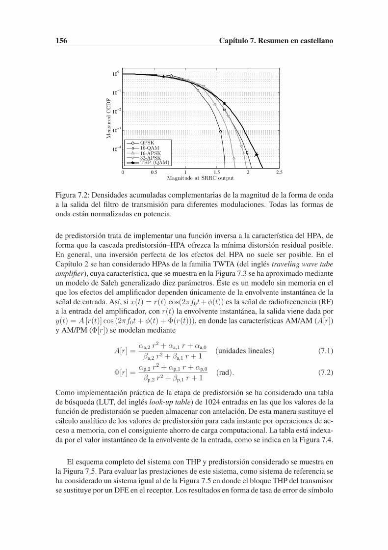
156 Capıtulo 7. Resumen en castellano
0 0.5 1 1.5 2 2.5
10−4
10−3
10−2
10−1
100
Magnitude at SRRC output
Mea
sure
dC
CD
F
QPSK16-QAM16-APSK32-APSKTHP (QAM)
Figura 7.2: Densidades acumuladas complementarias de la magnitud de la forma de onda
a la salida del filtro de transmision para diferentes modulaciones. Todas las formas de
onda estan normalizadas en potencia.
de predistorsion trata de implementar una funcion inversa a la caracterıstica del HPA, de
forma que la cascada predistorsion–HPA ofrezca la mınima distorsion residual posible.
En general, una inversion perfecta de los efectos del HPA no suele ser posible. En el
Capıtulo 2 se han considerado HPAs de la familia TWTA (del ingles traveling wave tube
amplifier), cuya caracterıstica, que se muestra en la Figura 7.3 se ha aproximado mediante
un modelo de Saleh generalizado diez parametros. Este es un modelo sin memoria en el
que los efectos del amplificador dependen unicamente de la envolvente instantanea de la
senal de entrada. Ası, si x(t) = r(t) cos(2πf0t+φ(t)) es la senal de radiofrecuencia (RF)
a la entrada del amplificador, con r(t) la envolvente instantanea, la salida viene dada por
y(t) = A [r(t)] cos (2πf0t+ φ(t) + Φ(r(t))), en donde las caracterısticas AM/AM (A[r])y AM/PM (Φ[r]) se modelan mediante
A[r] =αa,2 r
2 + αa,1 r + αa,0
βa,2 r2 + βa,1 r + 1(unidades lineales) (7.1)
Φ[r] =αp,2 r
2 + αp,1 r + αp,0
βp,2 r2 + βp,1 r + 1(rad). (7.2)
Como implementacion practica de la etapa de predistorsion se ha considerado una tabla
de busqueda (LUT, del ingles look-up table) de 1024 entradas en las que los valores de la
funcion de predistorsion se pueden almacenar con antelacion. De esta manera sustituye el
calculo analıtico de los valores de predistorsion para cada instante por operaciones de ac-
ceso a memoria, con el consiguiente ahorro de carga computacional. La tabla esta indexa-
da por el valor instantaneo de la envolvente de la entrada, como se indica en la Figura 7.4.
El esquema completo del sistema con THP y predistorsion considerado se muestra en
la Figura 7.5. Para evaluar las prestaciones de este sistema, como sistema de referencia se
ha considerado un sistema igual al de la Figura 7.5 en donde el bloque THP del transmisor
se sustituye por un DFE en el receptor. Los resultados en forma de tasa de error de sımbolo

7.1. Aplicacion de THP a la transmision punto a punto por satelite 157
−20 −15 −10 −5 0 5 10−15
−10
−5
0
IBO (dB)
OB
O(d
B)
Phase
(deg
)
0
10
20
30
40
50
60
AM/AM
AM/PM
Figura 7.3: Caracterısticas AM/AM y AM/PM consideradas para el TWTA a bordo del
satelite.
Figura 7.4: Esquema de la etapa de predistorsion considerada implementada mediante una
tabla de busqueda indexada por el valor de potencia instantanea de la senal de entrada..
Figura 7.5: Esquema del sistema propuesto que combina THP y predistorsion.

158 Capıtulo 7. Resumen en castellano
(SER, del ingles symbol error rate) de ambos sistemas se muestran en la Figura 7.6,
para diferentes valores de IBO. Como se puede observar, el empleo de predistorsion es
0 5 10 15 20
10-4
10-3
10-2
10-1
100
DFE, 16QAM mapping, TWTA amplifier
Eb/N
0 (dB)
SE
R
ZF, Linear Channel
uMMSE, Linear Channel
uMMSE, IBO=2dB
uMMSE, IBO=5dB
uMMSE, IBO=10dB
uMMSE, IBO=2dB, Predistortion
uMMSE, IBO=5dB, Predistortion
uMMSE, IBO=10dB, Predistortion
(a)
0 5 10 15 20
10-4
10-3
10-2
10-1
100
THP, 16QAM mapping, TWTA amplifier
Eb/N
0 (dB)
SE
R
ZF, Linear Channel
uMMSE, Linear Channel
uMMSE, IBO=2dB
uMMSE, IBO=5dB
uMMSE, IBO=10dB
uMMSE, IBO=2dB, Predistortion
uMMSE, IBO=5dB, Predistortion
uMMSE, IBO=10dB, Predistortion
(b)
Figura 7.6: Prestaciones en terminos de SER no codificada para (a) predistorsion combi-
nada con DFE, y (b) THP combinada con predistortion.
claramente positivo en los dos sistemas. Por otra parte, el sistema con DFE se ve menos
afectado por la distorsion no lineal residual que el sistema con THP. Esto se explica por la
distribucion de densidad de la senal precodificada, que como se muestra en la Figura 7.2
genera una forma de onda con un valor de pico de amplitude muy alto. Sin embargo, la
modulacion QAM (que es la empleada en el sistema con DFE) ofrece un valor de pico
menor que THP, y por ello la SER obtenida para un mismo IBO es menor para DFE que
para THP.
Este resultado sugiere que para mejorar las prestaciones del sistema con THP se de-
be reducir la amplitud de pico de la senal precodificada. Esto se puede conseguir con el
uso de tecnicas de “moldeado de senal”, comunmente conocidas como signal shaping,
que consiguen modificar la distribucion de densidad de los sımbolos transmitidos de cara
a mejorar alguna caracterıstica de la senal [59]. Tradicionalmente, el objetivo del signal
shaping ha sido la minimizacion de la energıa media de la secuencia transmitida, aunque
en general es una tecnica flexible que permite alcanzar otros objetivos. La combinacion
de signal shaping con THP no es sencilla: no basta con concatenar ambas operaciones,
sino que ambas tareas se deben realizar en una unica operacion. Esto se puede conseguir
mediante dos tecnicas distintas: trellis shaping y shaping sin barajado (en ingles, shaping
without scrambling) [59]. La tecnica escogida en el Capıtulo 2 ha sido el shaping sin ba-
rajado debido a que no obliga a realizar modificaciones en el receptor THP, mientras que
trellis shaping sı requiere de un receptor especıfico. En shaping sin barajado se emplea un
decodificador de Viterbi para escoger la secuencia precodificada que minimice una metri-
ca particular. La metrica se disena de forma que la senal precodificada resultante presente
ciertas caracterısticas deseadas (como por ejemplo la mınima energıa media transmitida).
En el segundo sistema propuesto en el Capıtulo 2 el transmisor implementa shaping
sin barajado y la misma etapa de predistorsion considerada anteriormente. Los resultados
obtenidos en terminos de tasa de error de bit (BER, del ingles bit error rate) se recogen en
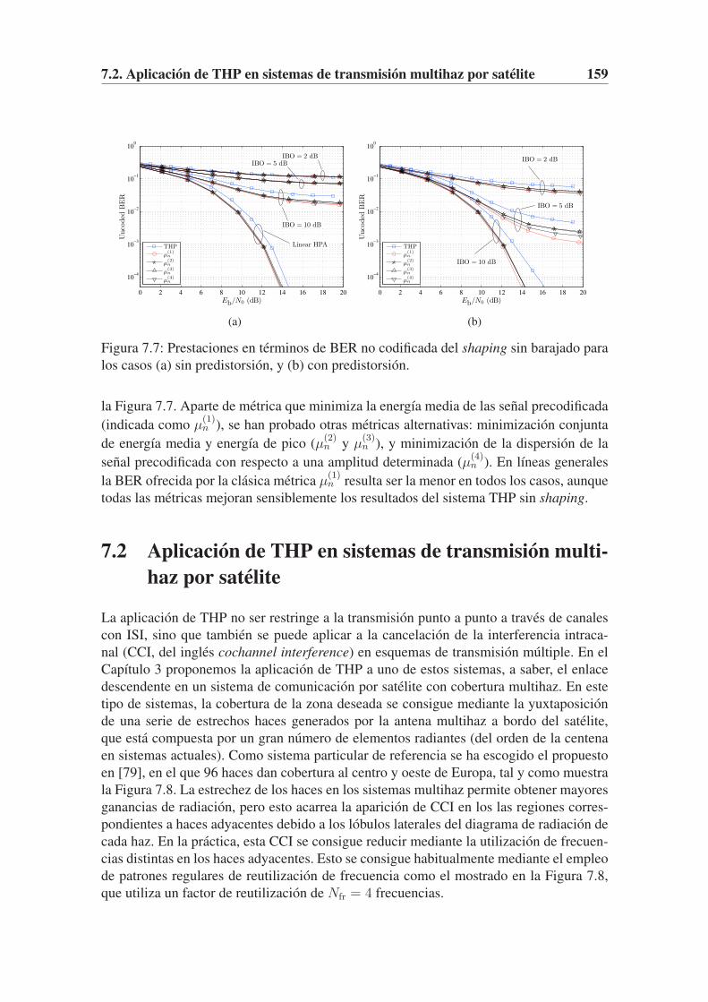
7.2. Aplicacion de THP en sistemas de transmision multihaz por satelite 159
0 2 4 6 8 10 12 14 16 18 20
10−4
10−3
10−2
10−1
100
Eb/N0 (dB)
Unco
ded
BE
R
Linear HPA
IBO = 10 dB
IBO = 5 dBIBO = 2 dB
THP
µ(1)n
µ(2)n
µ(3)n
µ(4)n
(a)
0 2 4 6 8 10 12 14 16 18 20
10−4
10−3
10−2
10−1
100
Eb/N0 (dB)
Unco
ded
BE
R
IBO = 10 dB
IBO = 5 dB
IBO = 2 dB
THP
µ(1)n
µ(2)n
µ(3)n
µ(4)n
(b)
Figura 7.7: Prestaciones en terminos de BER no codificada del shaping sin barajado para
los casos (a) sin predistorsion, y (b) con predistorsion.
la Figura 7.7. Aparte de metrica que minimiza la energıa media de las senal precodificada
(indicada como µ(1)n ), se han probado otras metricas alternativas: minimizacion conjunta
de energıa media y energıa de pico (µ(2)n y µ
(3)n ), y minimizacion de la dispersion de la
senal precodificada con respecto a una amplitud determinada (µ(4)n ). En lıneas generales
la BER ofrecida por la clasica metrica µ(1)n resulta ser la menor en todos los casos, aunque
todas las metricas mejoran sensiblemente los resultados del sistema THP sin shaping.
7.2 Aplicacion de THP en sistemas de transmision multi-
haz por satelite
La aplicacion de THP no ser restringe a la transmision punto a punto a traves de canales
con ISI, sino que tambien se puede aplicar a la cancelacion de la interferencia intraca-
nal (CCI, del ingles cochannel interference) en esquemas de transmision multiple. En el
Capıtulo 3 proponemos la aplicacion de THP a uno de estos sistemas, a saber, el enlace
descendente en un sistema de comunicacion por satelite con cobertura multihaz. En este
tipo de sistemas, la cobertura de la zona deseada se consigue mediante la yuxtaposicion
de una serie de estrechos haces generados por la antena multihaz a bordo del satelite,
que esta compuesta por un gran numero de elementos radiantes (del orden de la centena
en sistemas actuales). Como sistema particular de referencia se ha escogido el propuesto
en [79], en el que 96 haces dan cobertura al centro y oeste de Europa, tal y como muestra
la Figura 7.8. La estrechez de los haces en los sistemas multihaz permite obtener mayores
ganancias de radiacion, pero esto acarrea la aparicion de CCI en los las regiones corres-
pondientes a haces adyacentes debido a los lobulos laterales del diagrama de radiacion de
cada haz. En la practica, esta CCI se consigue reducir mediante la utilizacion de frecuen-
cias distintas en los haces adyacentes. Esto se consigue habitualmente mediante el empleo
de patrones regulares de reutilizacion de frecuencia como el mostrado en la Figura 7.8,
que utiliza un factor de reutilizacion de Nfr = 4 frecuencias.

160 Capıtulo 7. Resumen en castellano
Figura 7.8: Cobertura y distribucion de haces en el sistema multihaz considerado. Los
cuatro colores representan el factor de reutilizacion de frecuencia Nfr = 4 propuesto
en [79].
En el sistema estudiado en el Capıtulo 3 se supone que existe un solo terminal receptor
con una antena directiva en cada uno de los NB haces. Los receptores no cooperan entre
sı. Independientemente del factor de reutilizacion de frecuencia empleado, cada receptor
recibira, ademas de la senal correspondiente al propio haz, las senales no deseadas, aunque
atenuadas, correspondientes a los demas haces, como se representa en el esquema de la
Figura 7.9. Utilizando notacion vectorial como es habitual cuando se trata de transmision
multiple con salida simple (MISO, del ingles multiple-input single-output), el modelo de
senal para el sistema considerado se puede escribir como
yn = Han +wn (7.3)
en donde yn agrupa las senales recibidas por los terminales en el instante n, an agrupa
los sımbolos transmitidos por cada haz, wn es ruido aditivo blanco gaussiano, y H es
la matriz que representa el comportamiento del canal como filtro espacial: modela las
combinaciones lineales de los distintos haces que recibe cada terminal. Por ejemplo la
senal recibida por el terminal i-esimo se puede escribir como
[yn]i =
NTx∑
j=1
hij [an]j + [wn]i = hii [an]i +
NB∑
j=1j 6=i
hij [an]j + [wn]i (7.4)
en donde el segundo termino por la derecha representa la CCI recibida por el i-esimo
terminal.
Al igual que el caso punto a punto del Capıtulo 2, THP para transmision MISO es
una operacion no lineal (debido de nuevo a la operacion modulo) que tiene su equivalente
lineal conocido como precodificacion lineal. La figura 7.10 representa el esquema general
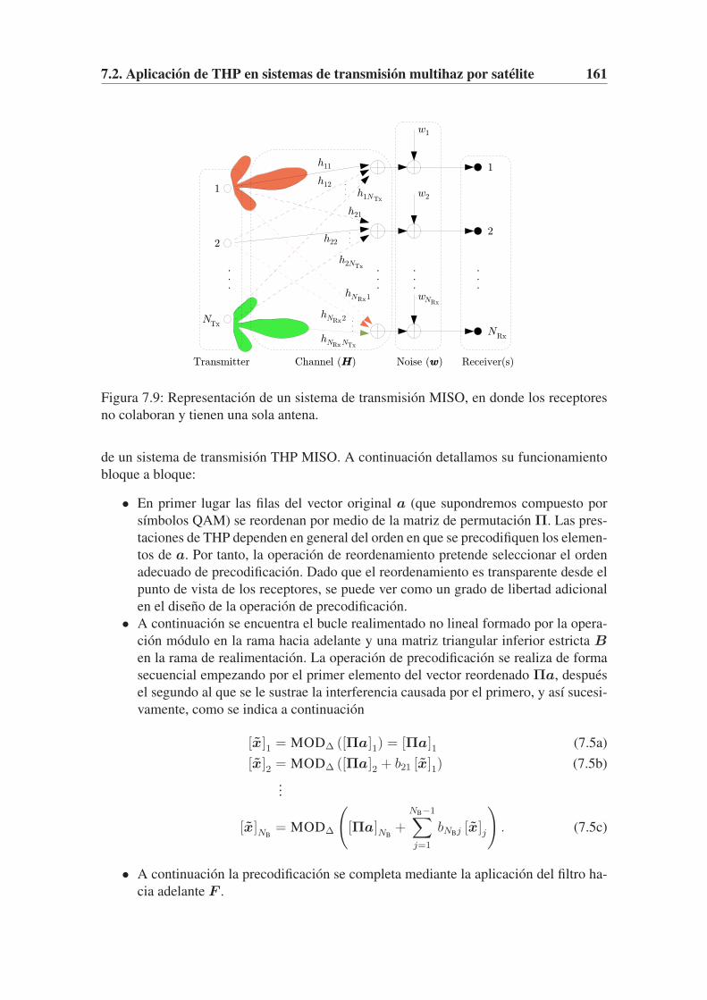
7.2. Aplicacion de THP en sistemas de transmision multihaz por satelite 161
Figura 7.9: Representacion de un sistema de transmision MISO, en donde los receptores
no colaboran y tienen una sola antena.
de un sistema de transmision THP MISO. A continuacion detallamos su funcionamiento
bloque a bloque:
• En primer lugar las filas del vector original a (que supondremos compuesto por
sımbolos QAM) se reordenan por medio de la matriz de permutacion Π. Las pres-
taciones de THP dependen en general del orden en que se precodifiquen los elemen-
tos de a. Por tanto, la operacion de reordenamiento pretende seleccionar el orden
adecuado de precodificacion. Dado que el reordenamiento es transparente desde el
punto de vista de los receptores, se puede ver como un grado de libertad adicional
en el diseno de la operacion de precodificacion.
• A continuacion se encuentra el bucle realimentado no lineal formado por la opera-
cion modulo en la rama hacia adelante y una matriz triangular inferior estricta B
en la rama de realimentacion. La operacion de precodificacion se realiza de forma
secuencial empezando por el primer elemento del vector reordenado Πa, despues
el segundo al que se le sustrae la interferencia causada por el primero, y ası sucesi-
vamente, como se indica a continuacion
[x]1 = MOD∆ ([Πa]1) = [Πa]1 (7.5a)
[x]2 = MOD∆ ([Πa]2 + b21 [x]1) (7.5b)
...
[x]NB= MOD∆
(
[Πa]NB+
NB−1∑
j=1
bNBj [x]j
)
. (7.5c)
• A continuacion la precodificacion se completa mediante la aplicacion del filtro ha-
cia adelante F .
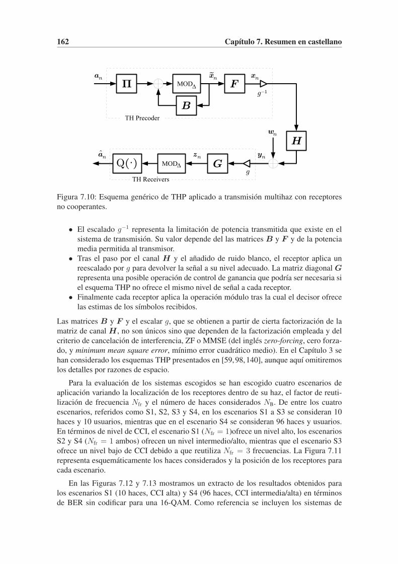
162 Capıtulo 7. Resumen en castellano
Figura 7.10: Esquema generico de THP aplicado a transmision multihaz con receptores
no cooperantes.
• El escalado g−1 representa la limitacion de potencia transmitida que existe en el
sistema de transmision. Su valor depende del las matrices B y F y de la potencia
media permitida al transmisor.
• Tras el paso por el canal H y el anadido de ruido blanco, el receptor aplica un
reescalado por g para devolver la senal a su nivel adecuado. La matriz diagonal G
representa una posible operacion de control de ganancia que podrıa ser necesaria si
el esquema THP no ofrece el mismo nivel de senal a cada receptor.
• Finalmente cada receptor aplica la operacion modulo tras la cual el decisor ofrece
las estimas de los sımbolos recibidos.
Las matrices B y F y el escalar g, que se obtienen a partir de cierta factorizacion de la
matriz de canal H , no son unicos sino que dependen de la factorizacion empleada y del
criterio de cancelacion de interferencia, ZF o MMSE (del ingles zero-forcing, cero forza-
do, y minimum mean square error, mınimo error cuadratico medio). En el Capıtulo 3 se
han considerado los esquemas THP presentados en [59,98,140], aunque aquı omitiremos
los detalles por razones de espacio.
Para la evaluacion de los sistemas escogidos se han escogido cuatro escenarios de
aplicacion variando la localizacion de los receptores dentro de su haz, el factor de reuti-
lizacion de frecuencia Nfr y el numero de haces considerados NB. De entre los cuatro
escenarios, referidos como S1, S2, S3 y S4, en los escenarios S1 a S3 se consideran 10
haces y 10 usuarios, mientras que en el escenario S4 se consideran 96 haces y usuarios.
En terminos de nivel de CCI, el escenario S1 (Nfr = 1)ofrece un nivel alto, los escenarios
S2 y S4 (Nfr = 1 ambos) ofrecen un nivel intermedio/alto, mientras que el escenario S3
ofrece un nivel bajo de CCI debido a que reutiliza Nfr = 3 frecuencias. La Figura 7.11
representa esquematicamente los haces considerados y la posicion de los receptores para
cada escenario.
En las Figuras 7.12 y 7.13 mostramos un extracto de los resultados obtenidos para
los escenarios S1 (10 haces, CCI alta) y S4 (96 haces, CCI intermedia/alta) en terminos
de BER sin codificar para una 16-QAM. Como referencia se incluyen los sistemas de

7.3. Estimacion de SNR 163
S1 S2
S3 S4
Figura 7.11: Haces considerados (circunferencias rojas) y posicion de los receptores (pun-
tos negros) en los escenarios S1, S2, S3, and S4. Los haces de color gris no causan inter-
ferencia.
precodificacion lineal ZF y MMSE [99]. En lıneas generales, se observa que los esque-
mas MMSE son mejore que los ZF para SNRs bajas, y sobre todo, que THP ofrece unas
prestaciones muy superiores a la precodificacion no lineal. Por ejemplo, para el escena-
rio S1 el mejor sistema THP alcanza una BER de 10−4 para Eb/N0 = 23 dB, mientras
que los esquemas lineales necesitan Eb/N0 = 34 dB para alcanzar la misma BER. Esta
diferencia, que aparece en mayor o menor medida siempre que el nivel de CCI no es des-
preciable, se debe a la penalizacion de de potencia transmitida que sufren las tecnicas de
precodificacion lineal.
Recientemente, en [43, 67] se ha estudiado la aplicacion de precodificacion lineal a
escenarios multihaz similares a los considerados en este capıtulo, con resultados prome-
tedores en terminos de disponibilidad y tasa de transmision agregada del sistema. Al igual
que THP, la precodificacion lineal alcanza a eliminar la CCI sin necesidad de reutilizar
frecuencias adicionales, lo cual aumenta la capacidad de transmision potencial del sis-
tema. El hecho de que THP evite la penalizacion de potencia transmitida propia de la
precodificacion lineal, sugiere que el empleo de THP aportarıa beneficios aun mayores
en terminos de capacidad de transmision del sistema que los ofrecidos por los sistemas
estudiados en [43, 67].
7.3 Estimacion de SNR
El Capıtulo 4 se proponen metodos de estimacion de la SNR aplicables en principio en
un rango amplio de situaciones practicas. La estimacion de SNR es necesaria en muchos
de los actuales sistemas de comunicaciones que implementan codificacion blanda [153],
esquemas de control de potencia o de codificacion y modulacion adaptativa [4, 17]. Exis-
te una gran variedad de estimadores de SNR que responde a distintas condiciones de

164 Capıtulo 7. Resumen en castellano
−5 0 5 10 15 20 25 30 35
10−4
10−3
10−2
10−1
100
Scenario 1 (10 ×10), 16-QAM
Eb/N0 (dB)
Unco
ded
BE
R
No PrecodingZF-LPMMSE-LPZF-THP-Fi ord.ZF-THP-JoMMSE-THP-JoZF-THP-Sa
Figura 7.12: BER sin codificar de los sistemas de precodificacion considerados para el
escenario S1 y modulacion 16-QAM.
−5 0 5 10 15 20 25 30 35
10−4
10−3
10−2
10−1
100
Scenario S4 (96 ×96), 16-QAM
Eb/N0 (dB)
Unco
ded
BE
R
No PrecodingZF-LPMMSE-LPZF-THP-Fi ord.ZF-THP-JoMMSE-THP-Jo
Figura 7.13: BER sin codificar de los sistemas de precodificacion considerados para el
escenario S4 y modulacion 16-QAM.

7.3. Estimacion de SNR 165
aplicacion. Los estimadores considerados en el Capıtulo 4 son estimadores que operan
a tasa de sımbolo y no ayudados por datos (NDA, del ingles non-data aided) principal-
mente. Existen otro tipo de estimadores que operan a partir de senales sobremuestrea-
das [131,136,143], o con conocimiento de los datos (DA, del ingles data-aided). De entre
los estimadores NDA, el capıtulo se centra principalmente en los estimadores basados
en la envolvente de las senal (EVB, del ingles envelope-based). Dentro de los estima-
dores EVB, los estimadores basados en momentos representan opciones atractivas dada
su sencillez de implementacion. Como ejemplos de estos estimadores se pueden citar el
estimador M1M2 [23] o el estimador M2M4 [118] que utilizan los momentos M1, M2
y M4. Estos estimadores funcionan bien para modulaciones de modulo constante (CM,
del ingles constant modulus) como las PSK, pero sus prestaciones se degradan para mo-
dulaciones con varios niveles (APSK, QAM). Recientemente se han propuesto algunos
estimadores nuevos basados en momentos que mejoran a los anteriores cuando se aplican
a dichas constelaciones. En particular, en [110] se presenta un nuevo estimador basado
en los momentos M2, M4 y M6 cuyas prestaciones mejoran mucho las de M2M4 para
constelaciones de dos niveles.
Asumiendo un modelo estatico de senal con desvanecimiento plano, y con sincroniza-
cion perfecta de portadora y muestreo, las muestras a tasa de sımbolo a la salida del filtro
adaptado vienen dadas por
rk =√Sxk + nk, k = 1, . . . , K (7.6)
siendo xk los sımbolos complejos transmitidos, nk las muestras de ruido blanco gaussiano
complejo circular con varianza desconocida N , y√S la ganancia desconocida del canal.
Los sımbolos xk pertenecen a una constelacion con I amplitudes, con Ri y Pi la amplitude
i-esima y su probabilidad asociada. Los momentos de la constelacion se definen como
cp.= E {|xk|p} =
∑Ii=1 PiR
pi . Los momentos muestrales de la envolvente, que se calculan
como
Mp.=
1
K
K∑
k=1
|rk|p, (7.7)
son estimadores insesgados de los momentos verdaderos de la envolvente, que en general
vienen dados por
Mp.= E {|rk|p}
= Np
2
I∑
i=1
PiΓ(p
2+ 1)
e−ρR2i1F1
(p
2+ 1; 1; ρR2
i
)
(7.8)
siendo ρ la SNR en unidades naturales, Γ(·) la funcion gamma y 1F1(·; ·; ·) la funcion
hipergeometrica confluente. Para orden p par (7.8) admite una expresion mas sencilla que
depende de ρ, N y los momentos de la constelacion [86, 110]:
M2n = Nn
n∑
m=0
(n!)2
(n−m)!(m!)2c2mρ
m. (7.9)

166 Capıtulo 7. Resumen en castellano
Muchos de los estimadores basados en momentos se construyen a partir de cocientes de
potencias de momentos en donde N se cancela. Por ejemplo, en [68] se propone la familia
de funciones
fk,l(ρ).=
M lk
Mkl
, para k 6= l (7.10)
a partir de la cual, empleando momentos muestrales en lugar de los verdaderos, se obtie-
nen las estimas de SNR mediante inversion de (7.10)
ρk,l = f−1k,l
(
M lk
Mkl
)
. (7.11)
En la Seccion 4.3 se propone una nueva familia de estimadores basada en cocientes de
momentos que generaliza tanto la familia propuesta en [68] como el estimador de sexto
orden propuesto en [110]. La familia propuesta se compone de combinaciones lineales de
cocientes de la forma
f(ρ).=
(U∏
i=1
Mpi2ni
)/
MQ2 , ni, pi ∈ N (7.12)
en donde Q =∑U
i=1 nipi para cumplir que N desaparece del cociente (2Q es el orden
estadıstico del cociente). Estos cocientes se componen exclusivamente de momentos de
orden par, y presentan la propiedad de que tras aplicar el cambio de variable z = ρ/(1+ρ)(SNR normalizada), pueden reducirse a un polinomio F (z) de orden Q. En particular, en
la Seccion 4.3 se propone el estimador compuesto de todos los cocientes de esta familia
de orden igual o inferior a 8:
fEOS(ρ).= β
M4
M22
+ γM6
M32
+ δM2
4
M42
+ ǫM8
M42
(7.13)
siendo α = [β γ δ ǫ]T ∈ R4 el vector de pesos de la combinacion lineal. Este estimador
generaliza otros anteriores como M2M4, que se construye a partir de f(ρ) = M4/M22 , o
el estimador de sexto orden propuesto en [110], que se extrae de f(ρ) = −bM4/M22 +
M6/M32 . La combinacion lineal (7.13) se puede reducir a
FEOS(z) = F4 z4 + F3 z
3 + F2 z2 + F0 (7.14)
en donde los coeficientes Fi son funciones exclusivas de los momentos de la constelacion
y de los pesos de α. El estimador de la SNR normalizada z ∈ (0, 1) viene dado por la
solucion de
FEOS(z) = βM4
M22
+ γM6
M32
+ δM2
4
M42
+ ǫM8
M42
= hEOS(m) (7.15)
con m.= [M2 M4 M6 M8]
T ∈ R4 el vector de momentos muestrales. Para encontrar la
estima se puede aplicar el metodo algebraico de calculo de raıces de polinomios de cuarto
grado [1, pp.18-19], o bien optar por un metodo iterativo, como por ejemplo:
z(0) = 1, z(n+1) =
√
hEOS(m)− F0
F4(z(n))2 + F3 z(n) + F2
. (7.16)

7.3. Estimacion de SNR 167
El analisis estadıstico del estimador basado en aproximaciones de Taylor ofrece que
la varianza, Var {ρ} y el sesgo Bias {ρ} vienen dados por
Var {ρ} ≈ vTCv =1
K
∑10n=0A
(Var)n ρn
∑6n=2B
(Var)n ρn
(7.17)
Bias {ρ} ≈ 1
2Tr (HC) =
1
KL(ρ) + J(ρ) Var {ρ} =
1
K
∑12n=0A
(Bias)n ρn
∑9n=3B
(Bias)n ρn
(7.18)
en donde C es la matriz de covarianza de m, v y H dependen de α, ρ y los momentos
de la constelacion, al igual que los cocientes de polinomios L(ρ).= A(L)(ρ)/B(L)(ρ),
con A(L)(ρ) =∑6
n=0A(L)n ρn, B(L)(ρ) =
∑4n=1B
(L)n ρn, y J(ρ)
.= A(J)(ρ)/B(L)(ρ), con
A(J)(ρ) =∑3
n=0A(J)n ρn. Los polinomios A(Var)(ρ), B(Var)(ρ) son cuadraticos en α, mien-
tras que A(L)(ρ), B(L)(ρ) y A(J)(ρ) son lineales en α.
En general, tanto la varianza como el sesgo son funciones de los momentos de la cons-
telacion y los pesos α, ademas de la SNR ρ. Por tanto, α representa un conjunto de grados
de libertad en el diseno del estimador. Parece logico emplear dichos grados de libertad en
optimizar las prestaciones del estimador resultante en terminos de sesgo y varianza. Para
ello, en la Seccion 4.3 se proponen dos criterios de optimizacion alternativos:
• C1: optimizacion para SNR alta. Usar un grado de libertad en α en anular el
coeficiente de mayor orden de L(ρ), y el resto en minimizar el coeficiente de mayor
orden de Var {ρ}. Si este se puede anular, y sobran grados de libertad, usar estos en
minimizar el siguiente coeficiente de Var {ρ}, y ası sucesivamente.
• C2: optimizacion para un valor nominal de SNR. Dado un valor particular de la
SNR ρ0, minimizar la varianza (7.17) bajo la restriccion de que L(ρ) en (7.18) sea
cero.
La aplicacion de estos criterios permite obtener estimadores cuyas prestaciones para
constelaciones de varios niveles mejoran sustancialmente la de los estimadores previos
basados en momentos. Por ejemplo, los resultados para una constelacion 16-APSK (dos
niveles) se muestran en la Figura 7.14, tanto en sus valores teoricos como empıricos ob-
tenidos mediante simulacion.
En la Seccion 4.4 se trata del problema de estimar la SNR a partir de conjuntos de
muestras pertenecientes a varias constelaciones. Este caso puede darse por ejemplo si se
pretende estimar la SNR a partir de las muestras de una trama DVB-S2 [54], en donde
los sımbolos de la cabecera y los sımbolos pilotos pertenecen a una constelacion distinta
a la empleada para los datos (trama heterogenea), como se puede ver en la Figura 7.15 El
modelo de senal viene dado por
rk =√Sxk + nk, k ∈ {1, . . . , K} = K1 ∪ K2 (7.19)
en donde K1 y K2 son conjuntos disjuntos de ındices que indexan los sımbolos de la trama
que pertenecen a dos constelaciones distintas, y son conocidos por el receptor. (7.6)
Para estimar la SNR a partir de esta trama, podrıa plantearse el empleo de un estimador
NDA directamente sobre toda la trama, o bien sobre los sımbolos de una de las subtramas.
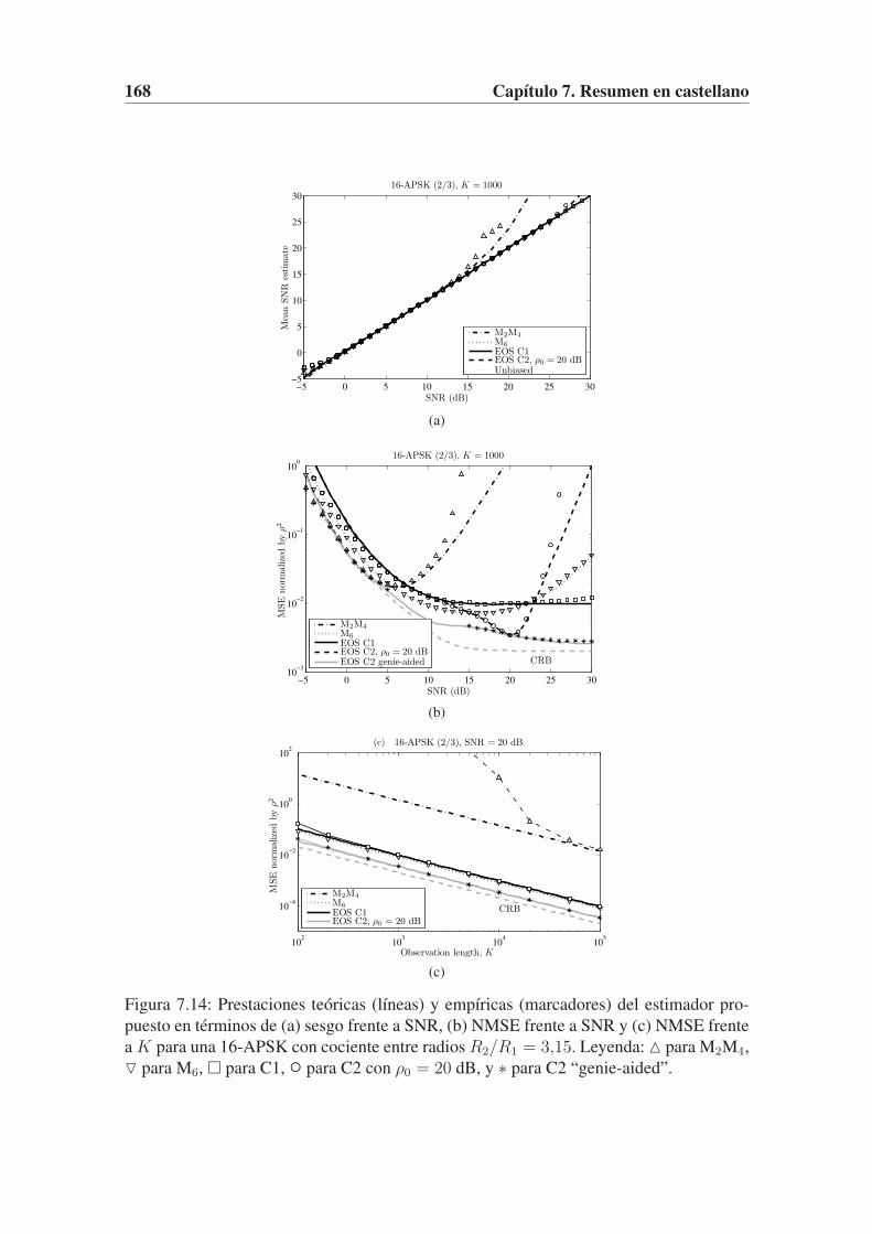
168 Capıtulo 7. Resumen en castellano
−5 0 5 10 15 20 25 30−5
0
5
10
15
20
25
30
SNR (dB)
Mea
nSN
Res
tim
ate
16-APSK (2/3), K = 1000
M2M4M6EOS C1EOS C2, ρ0 = 20 dBUnbiased
(a)
−5 0 5 10 15 20 25 3010
−3
10−2
10−1
100
SNR (dB)
MSE
nor
mal
ized
by
ρ2
16-APSK (2/3), K = 1000
CRB
M2M4M6EOS C1EOS C2, ρ0 = 20 dBEOS C2 genie-aided
(b)
102
103
104
105
10−4
10−2
100
102
Observation length, K
MSE
nor
mal
ized
by
ρ2
(c) 16-APSK (2/3), SNR = 20 dB
CRB
M2M4M6EOS C1EOS C2, ρ0 = 20 dB
(c)
Figura 7.14: Prestaciones teoricas (lıneas) y empıricas (marcadores) del estimador pro-
puesto en terminos de (a) sesgo frente a SNR, (b) NMSE frente a SNR y (c) NMSE frente
a K para una 16-APSK con cociente entre radios R2/R1 = 3,15. Leyenda: △ para M2M4,
▽ para M6, � para C1, ◦ para C2 con ρ0 = 20 dB, y ∗ para C2 “genie-aided”.

7.4. Estimacion de fase para modulaciones QAM en cruz 169
Figura 7.15: Ejemplo de una trama heterogenea que contiene sımbolos de dos constela-
ciones distintas A1, A2.
Ninguna de estas dos opciones serıa optima en el sentido de que no emplean toda la
informacion disponible. Por ello, en la Seccion 4.4 se proponen tres esquemas alternativos
de estimacion:
• Combinacion convexa de estimas, CCE (del ingles convex combination of es-
timates). En este esquema el estimador se construye a partir de dos estimado-
res distintos que se aplican cada uno a los sımbolos de una constelacion ρcce =λcce · ρ(1) + (1 − λcce) · ρ(2). Los estimadores de partida ρ(1) y ρ(2) pueden ser de
cualquier tipo, pero si son insesgados, el estimador resultante tambien lo sera. El
parametro λcce se puede optimizar para minimizar la varianza del estimador resul-
tante.
• Combinacion convexa de momentos, CCM (del ingles convex combination of
moments). En este esquema se utilizan estimadores basados en momentos que se
construyen a partir de momentos modificados. Estos momentos modificados son
combinaciones convexas de los momentos de cada uno de los dos subconjuntos:
M ccmn = λccm,n · M (1)
n + (1 − λccm,n) · M (2)n , en donde los parametros λccm,n se
pueden optimizar para minimizar la varianza resultante.
• Mınimos cuadrados ponderados, WLS (del ingles weighted least squares). Este
esquema busca un estimador a partir de los momentos M2 y M4 aplicados a cada
una de las dos subtramas. Las cuatro ecuaciones se combinan linealmente y de esa
combinacion se extrae un estimador de la SNR. Los pesos de la combinacion se
optimizan para minimizar la varianza.
En la Figura 7.16 se muestran los resultados obtenidos con los tres esquemas pro-
puestos para la estimacion a partir de una trama corta DVB-S2 formada por una QPSK
(162 sımbolos) y una 32-APSK (3240 sımbolos). En general, el esquema CCE, usando
los estimadores M2M4 y M6 para cada subtrama, ofrece con diferencia mucho mejores
prestaciones en terminos de sesgo y NMSE que los esquemas CCM y WLS. Ademas,
el esquema CCE presenta la flexibilidad de poderse emplear con cualesquier estimado-
res disponibles, incluyendo estimadores DA. El empleo de estimadores DA tiene interes
practico, dado que comunmente algunos de lo sımbolos en cada trama son conocidos
(inicio de trama, sımbolos pilotos). En la Figura 7.16c se representan las prestaciones del
esquema CCE que combina el estimador DA ML (SNORE) [66, 131] con M6.
7.4 Estimacion de fase para modulaciones QAM en cruz
El Capıtulo 5 propone dos estimadores NDA de fase para constelaciones QAM en cruz,
como por ejemplo la 32-QAM y la 128-QAM. Metodos NDA clasicos como los estima-

170 Capıtulo 7. Resumen en castellano
−5 0 5 10 15 20 25−5
0
5
10
15
20
25
SNR (dB)
Mea
nes
tim
ate
dva
lue
(dB
)
C1
CCE 24−6
CCE SNORE−6
CCM
WLS
Unbiased
(a)
−5 0 5 10 15 20 25
10−3
10−2
10−1
100
SNR (dB)
NM
SE
C1 NDA-NDA
NDA subframe 1
NDA subframe 2
NCRB subframes
NCRB full frame (NDA)
NVar. CCE 24−6
NMSE CCE 24−6
NMSE CCM
NMSE WLS
(b)
−5 0 5 10 15 20 25
10−3
10−2
10−1
100
SNR (dB)
NM
SE
C1 DA-NDA
DA subframe 1NDA subframe 2
NCRB subframes
NCRB full frame (DA−NDA)
Var. CCE SNORE−6
NMSE CCE SNORE−6
(c)
Figura 7.16: Prestaciones de los estimadores propuestos en terminos de (a) valor medio
estimado (a), y NMSEs para combinacion de estimadores (b) NDA y (c) DA-NDA. Se
muestran varianzas analıticas, CRBs normalizadas y NMSEs obtenidos mediante simula-
cion.
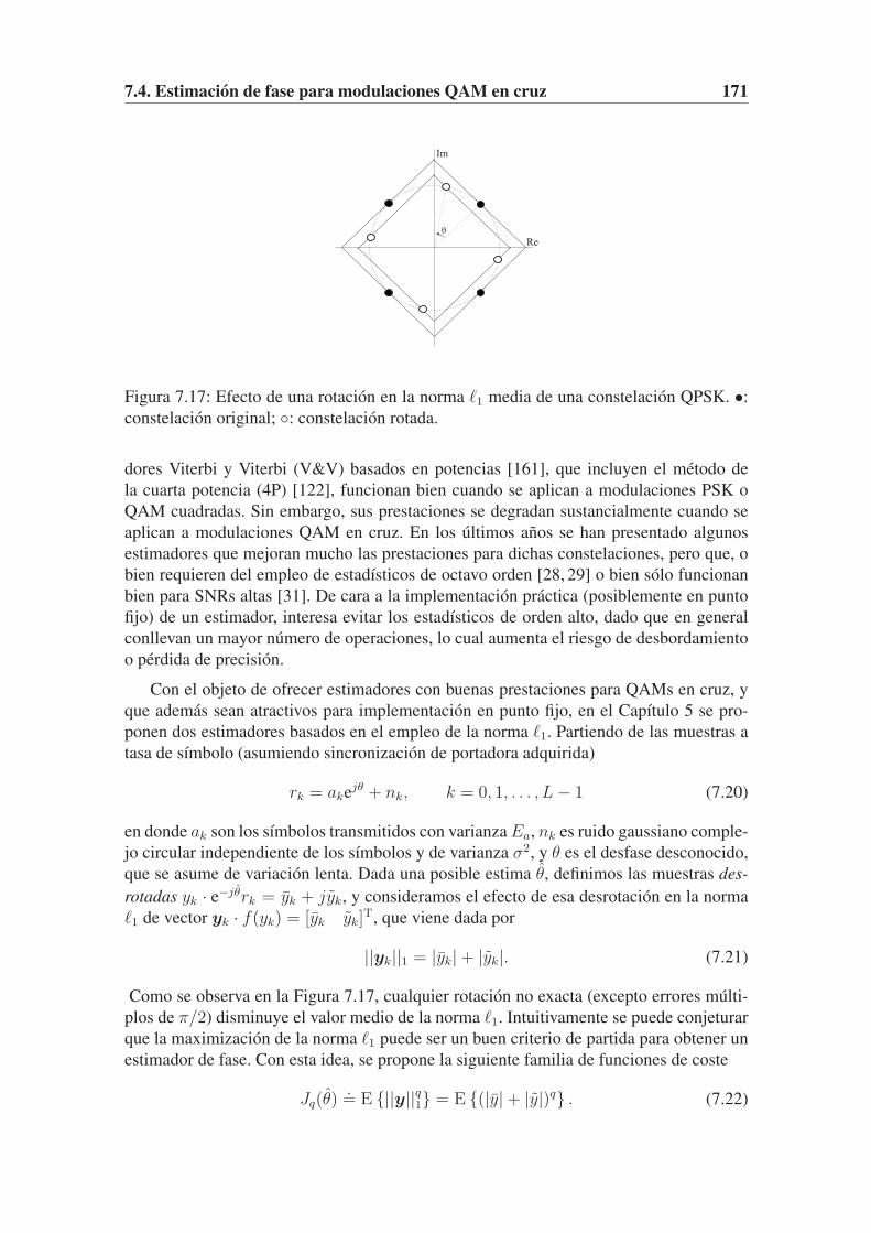
7.4. Estimacion de fase para modulaciones QAM en cruz 171
Figura 7.17: Efecto de una rotacion en la norma ℓ1 media de una constelacion QPSK. •:
constelacion original; ◦: constelacion rotada.
dores Viterbi y Viterbi (V&V) basados en potencias [161], que incluyen el metodo de
la cuarta potencia (4P) [122], funcionan bien cuando se aplican a modulaciones PSK o
QAM cuadradas. Sin embargo, sus prestaciones se degradan sustancialmente cuando se
aplican a modulaciones QAM en cruz. En los ultimos anos se han presentado algunos
estimadores que mejoran mucho las prestaciones para dichas constelaciones, pero que, o
bien requieren del empleo de estadısticos de octavo orden [28, 29] o bien solo funcionan
bien para SNRs altas [31]. De cara a la implementacion practica (posiblemente en punto
fijo) de un estimador, interesa evitar los estadısticos de orden alto, dado que en general
conllevan un mayor numero de operaciones, lo cual aumenta el riesgo de desbordamiento
o perdida de precision.
Con el objeto de ofrecer estimadores con buenas prestaciones para QAMs en cruz, y
que ademas sean atractivos para implementacion en punto fijo, en el Capıtulo 5 se pro-
ponen dos estimadores basados en el empleo de la norma ℓ1. Partiendo de las muestras a
tasa de sımbolo (asumiendo sincronizacion de portadora adquirida)
rk = akejθ + nk, k = 0, 1, . . . , L− 1 (7.20)
en donde ak son los sımbolos transmitidos con varianza Ea, nk es ruido gaussiano comple-
jo circular independiente de los sımbolos y de varianza σ2, y θ es el desfase desconocido,
que se asume de variacion lenta. Dada una posible estima θ, definimos las muestras des-
rotadas yk · e−jθrk = yk + jyk, y consideramos el efecto de esa desrotacion en la norma
ℓ1 de vector yk · f(yk) = [yk yk]T, que viene dada por
||yk||1 = |yk|+ |yk|. (7.21)
Como se observa en la Figura 7.17, cualquier rotacion no exacta (excepto errores multi-
plos de π/2) disminuye el valor medio de la norma ℓ1. Intuitivamente se puede conjeturar
que la maximizacion de la norma ℓ1 puede ser un buen criterio de partida para obtener un
estimador de fase. Con esta idea, se propone la siguiente familia de funciones de coste
Jq(θ).= E {||y||q1} = E {(|y|+ |y|)q} . (7.22)

172 Capıtulo 7. Resumen en castellano
La Figura 7.18 muestra la variacion de las funciones de coste con q = 1 y q = 2 para varias
constelaciones en cruz. Como se puede observar, J1 y J2 son funciones multimodales, con
un maximo absoluto para error de fase cero. 3 A partir de la maximizacion de J1 es posible
−40 −20 0 20 40
0.94
0.96
0.98
1
phase error (deg)
32-QAM
−40 −20 0 20 40
0.94
0.96
0.98
1
phase error (deg)
128-QAM
−40 −20 0 20 40
0.94
0.96
0.98
1
phase error (deg)
512-QAM
−40 −20 0 20 40
0.94
0.96
0.98
1
phase error (deg)
2048-QAM
Figura 7.18: Constelaciones QAM en cruz: comportamiento de las funciones de coste
basadas en la norma ℓ1 Jq(θ) (normalizadas por su valor maximo) en ausencia de ruido.
q = 1 (lınea continua) y 2 (lınea discontinua).
obtener el siguiente estimador
θ(1)n+1 = −arg
{L−1∑
k=0
csgn(
rk · e−jθ(1)n
)
· r∗k
}
. (7.23)
Asimismo, la maximizacion de J2 ofrece el siguiente estimador
sk(θ(2)n ) = sgn
(
Im{
r2ke−j2θ(2)n
})
, k = 0, . . . , L− 1 (7.24a)
θ(2)n+1 =
1
2arg
{L−1∑
k=0
[
r2ksk(θ(2)n )]}
− π
4. (7.24b)
Ambos estimadores dependen de una estima inicial θ(q)0 que ha de tomarse de algun esti-
mador existente, como por ejemplo, el estimador 4P [122] o el estimador de Cartwright de
octavo orden (C8) [29]. La estima ha de ser lo suficientemente buena como para colocar
la iteracion dentro del dominio de atraccion del maximo absoluto. Como se puede obser-
var, las operaciones realizadas por los estimadores (7.23) y (7.24) son como maximo de
segundo orden estadıstico, lo cual supone una ventaja apreciable respecto a 4P y C8 de
cara a la implementacion en punto fijo. En la Seccion 5.5 se obtienen las varianzas de
ambos estimadores para los casos asintoticos de SNR suficientemente alta y longitud de
las observaciones suficientemente larga.
Las prestaciones de ambos estimadores inicializados con 4P y C8 se muestran en la
Figura (7.19) para el caso de implementacion en punto flotante tras cinco iteraciones.
Como se puede observar ambos estimadores ofrecen un RMSE comparable (32-QAM)

7.4. Estimacion de fase para modulaciones QAM en cruz 173
10 15 20 25 300.5
1
1.5
2
2.5
3
3.5
4
Eb/N0 (dB)
RM
SE
(deg
)
32-QAM, θ = 20◦, L = 1024
(a)
10 15 20 25 300.5
1
1.5
2
2.5
3
Eb/N0 (dB)
RM
SE
(deg
)
128-QAM, θ = 20◦, L = 2048
(b)
Figura 7.19: RMSE frente a la SNR por bit para (a) 32-QAM y (b) 128-QAM. Leyenda:
4P (�), C8 (♦), J1 (×), J2 (◦). J1 y J2 se inicializan con 4P (lınea continua) y C8 (lınea
discontinua). Las lıneas finas discontinuas muestran los valores de RMSE teoricos de los
estimadores 4P, θ(1) y θ(2).
o incluso menor (128-QAM) que el ofrecido por el estimador C8, incluso cuando son
inicializados por la peor estima (4P).
Los mismos resultados, pero obtenidos con la implementacion en punto fijo, se mues-
tran en la Figura 7.20. Los resultados para la constelacion 32-QAM (con longitudes de
palabra de 12, 10 y 8 bits) dan muestra de la robustez de los metodos propuestos frente a
los existentes de mayor orden (4P y C8). A medida que disminuye la longitud de palabra,
los metodos de mayor orden dejan de funcionar correctamente, mientras que los metodos
iterativos propuestos se ven mucho menos afectados. Lo mismo se observa para el caso
de la 128-QAM.
Estos resultados permite concluir que los estimadores propuestos no solo mejoran las
prestaciones de sus inicializadores, sino que mantienen sus prestaciones en condiciones
exigentes de punto fijo, lo cual los hace atractivos de cara a la implementacion practica.
En cuanto a su inicializacion, se ha visto que los estimadores 4P y C8 funcionan razona-
blemente bie, aunque otros esquemas como los V&V o incluso esquemas DA (en el caso
de que el bloque de datos contenga sımbolos de entrenamiento) podrıan ser igualmente
utiles.
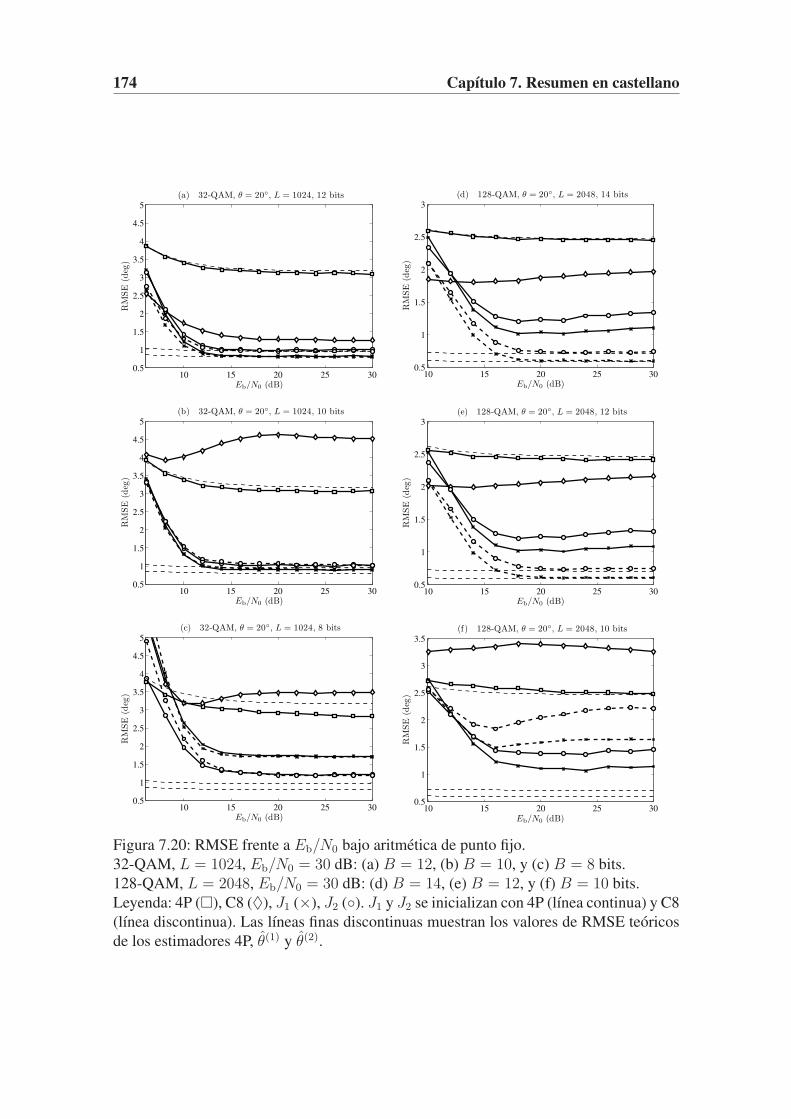
174 Capıtulo 7. Resumen en castellano
10 15 20 25 300.5
1
1.5
2
2.5
3
3.5
4
4.5
5
Eb/N0 (dB)
RM
SE
(deg
)
(a) 32-QAM, θ = 20◦, L = 1024, 12 bits
10 15 20 25 300.5
1
1.5
2
2.5
3
3.5
4
4.5
5
Eb/N0 (dB)
RM
SE
(deg
)
(b) 32-QAM, θ = 20◦, L = 1024, 10 bits
10 15 20 25 300.5
1
1.5
2
2.5
3
3.5
4
4.5
5
Eb/N0 (dB)
RM
SE
(deg
)
(c) 32-QAM, θ = 20◦, L = 1024, 8 bits
10 15 20 25 300.5
1
1.5
2
2.5
3
Eb/N0 (dB)
RM
SE
(deg
)
(d) 128-QAM, θ = 20◦, L = 2048, 14 bits
10 15 20 25 300.5
1
1.5
2
2.5
3
Eb/N0 (dB)
RM
SE
(deg
)(e) 128-QAM, θ = 20◦, L = 2048, 12 bits
10 15 20 25 300.5
1
1.5
2
2.5
3
3.5
Eb/N0 (dB)
RM
SE
(deg
)
(f ) 128-QAM, θ = 20◦, L = 2048, 10 bits
Figura 7.20: RMSE frente a Eb/N0 bajo aritmetica de punto fijo.
32-QAM, L = 1024, Eb/N0 = 30 dB: (a) B = 12, (b) B = 10, y (c) B = 8 bits.
128-QAM, L = 2048, Eb/N0 = 30 dB: (d) B = 14, (e) B = 12, y (f) B = 10 bits.
Leyenda: 4P (�), C8 (♦), J1 (×), J2 (◦). J1 y J2 se inicializan con 4P (lınea continua) y C8
(lınea discontinua). Las lıneas finas discontinuas muestran los valores de RMSE teoricos
de los estimadores 4P, θ(1) y θ(2).
Bibliography
[1] M. Abramowitz and I. Stegun, Eds., Handbook of Mathematical Functions, 9th ed.
New York: Dover, 1972.
[2] S. Abrar, “Blind carrier phase recovery in cross QAM communication systems,” in
Proc. International Conference on Emerging Technologies ICET ’06, 13–14 Nov.
2006, pp. 1–7.
[3] N. Alagha, “Cramer-Rao bounds of SNR estimates for BPSK and QPSK modulated
signals,” IEEE Commun. Lett., vol. 5, no. 1, pp. 10–12, Jan. 2001.
[4] G. Albertazzi, S. Cioni, G. Corazza, M. Neri, R. Pedone, P. Salmi, A. Vanelli-
Coralli, and M. Villanti, “On the adaptive DVB-S2 physical layer: Design and
performance,” IEEE Wireless Commun. Mag., vol. 12, no. 6, pp. 62–68, Dec. 2005.
[5] M. Alvarez-Dıaz, R. Lopez-Valcarce, and I. Gomez Alonso, “Blind ℓ1-norm-based phase estimation for cross-QAM robust to finite precision ef-
fects,” Signal Processing, accepted for publication, 2010. [Online]. Available:
http://dx.doi.org/10.1016/j.sigpro.2010.04.019
[6] M. Alvarez-Dıaz, R. Lopez-Valcarce, and C. Mosquera, “SNR estimation for mul-
tilevel constellations using higher-order moments,” IEEE Trans. Signal Process.,
vol. 58, no. 3, Part 2, pp. 1515–1526, March 2010.
[7] M. Alvarez-Dıaz, N. Courville, C. Mosquera, G. Liva, and G. E. Corazza, “Non-
linear interference mitigation for broadband multimedia satellite systems,” in
Proc. of International Workshop on Satellite and Space Communications 2007
(IWSSC’07), Salzburg, Austria, September 13-14 2007, pp. 61–65.
[8] M. Alvarez-Dıaz and R. Lopez-Valcarce, “Diamond contour-based phase recovery
for (cross)-QAM constellations,” in Proc. IEEE/SP 13th Workshop on Statistical
Signal Processing, Bourdeaux, France, July 17-20 2005, pp. 669–674.
[9] M. Alvarez-Dıaz, R. Lopez-Valcarce, and C. Mosquera, “SNR estimation with
heterogeneous frames,” in 4th Advanced Satellite Mobile Systems Conference,
Bologna, Italy, August 26-28 2008.

176 BIBLIOGRAPHY
[10] M. Alvarez-Dıaz, M. Neri, C. Mosquera, and G. E. Corazza, “Joint precoding and
predistortion techniques for satellite telecommunication systems,” in Proc. of In-
ternational Workshop on Satellite and Space Communications 2005 (IWSSC’05),
Siena, Italy, September 8-9 2005, pp. 688–692.
[11] ——, “Trellis shaping techniques for satellite telecommunication systems,” in
Proc. of International Workshop on Satellite and Space Communications 2006
(IWSSC’06), Leganes, Spain, September 14-15 2006, pp. 148–152.
[12] M. Alvarez-Dıaz, S. Scalise, G. Sciascia, R. Mura, P. Conforto, and H. Ernst,
“DVB-S air interface over railroad satellite channel: Performance and extensions,”
in Proc. of Sixth Baiona Workshop on Signal Processing in Communications,
Baiona, Spain, September 8-10 2003.
[13] P. Angeletti and N. Alagha, “Space/ground beamforming techniques for emerging
hybrid satellite terrestrial networks,” in Proc. 27th AAIA International Communi-
cations Satellite Systems Conference, Edinburgh, Scotland, UK, June 1–4 2009.
[14] P. Angeletti, G. Gallinaro, M. Lisi, and A. Vernucci, “On-ground digital beamform-
ing techniques for satellite smart antennas,” in Proc. 19th AIAA International Com-
munications Satellite Systems Conference, Toulouse, France, April 17–20 2001.
[15] P.-D. Arapoglou, Deliverable D1: Preliminary Selection of Most Promising MIMO
Techniques Applicable to Study Case 1. ESA Contract No. 21591/08/NL/AT,
Wireless & Satellite Communications Group, National Technical University of
Athens, 2009.
[16] R. E. Badra and B. Daneshrad, “Asymmetric physical layer design for high-speed
wireless digital communications,” IEEE J. Sel. Areas Commun., vol. 17, no. 10, pp.
1712–1724, Oct. 1999.
[17] K. Balachandran, S. R. Kadaba, and S. Nanda, “Channel quality estimation and
rate adaptation for cellular mobile radio,” IEEE J. Sel. Areas Commun., vol. 17,
no. 7, pp. 1244–1256, July 1999.
[18] F. Bellili, A. Stephenne, and S. Affes, “SNR estimation of QAM-modulated trans-
missions over time-varying SIMO channels,” in Proc. IEEE International Sympo-
sium on Wireless Communication Systems 2008 (ISWCS ’08), Reykjavik, Iceland,
21–24 Oct 2008, pp. 199–203.
[19] ——, “Cramer-Rao bound for NDA SNR estimates of square QAM modulated sig-
nals,” in Proc. IEEE Wireless Communications and Networking Conference WCNC
2009, 5–8 April 2009, pp. 1–5.
[20] ——, “Cramer-Rao lower bounds for subcarrier SNR estimates over multicarrier
channels,” IEEE Trans. Signal Process., vol. 58, no. 2, pp. 891–896, Feb. 2010.
[21] S. Benedetto and E. Biglieri, “Nonlinear equalization of digital satellite channels,”
IEEE J. Sel. Areas Commun., vol. 1, no. 1, pp. 57–62, Jan 1983.

BIBLIOGRAPHY 177
[22] S. Benedetto, E. Biglieri, and R. Daffara, “Modeling and performance evaluation of
nonlinear satellite links-A Volterra series approach,” IEEE Trans. Aerosp. Electron.
Syst., vol. AES-15, no. 4, pp. 494 –507, july 1979.
[23] T. Benedict and T. Soong, “The joint estimation of signal and noise from the sum
envelope,” IEEE Trans. Inf. Theory, vol. 13, no. 3, pp. 447–454, Jul 1967.
[24] T. Benjamin, M. Griffin, and W. W. Chapman, “Methods and systems for satel-
lite communications employing ground-based beam forming with spatially dis-
tributed hybrid matrix amplifiers,” U.S. Patent 2007/9 281 612 A1, December 6,
2007, patent application.
[25] D. Brandel, W. Watson, and A. Weinberg, “NASA’s advanced tracking and data
relay satellite system for the years 2000 and beyond,” Proc. IEEE, vol. 78, no. 7,
pp. 1141 –1151, jul 1990.
[26] C. Caini and G. Corazza, “Satellite downlink reception through intermediate mod-
ule repeaters: power delay profile analysis,” in Proc. EMPS/ASMS Conference,
ESA/ESTEC, Noordwijk, The Netherlands, September 21-22 2004.
[27] C. Caini, G. E. Corazza, G. Falciasecca, M. Ruggieri, and F. Vatalaro, “A spectrum-
and power-efficient EHF mobile satellite system to be integrated with terrestrial
cellular systems.” IEEE J. Sel. Areas Commun., vol. 10, no. 8, pp. 1315–1325,
1992.
[28] P. Campisi, G. Panci, S. Colonnese, and G. Scarano, “Blind phase recovery for
QAM communication systems,” IEEE Trans. Signal Process., vol. 53, no. 4, pp.
1348–1358, 2005.
[29] K. V. Cartwright, “Blind phase recovery in cross QAM communication systems
with eighth-order statistics,” IEEE Signal Process. Lett., vol. 8, no. 12, pp. 304–
306, Dec. 2001.
[30] K. V. Cartwright and E. J. Kaminsky, “Asymptotic performance of the Pth power-
law phase estimator,” in Proc. IEEE Global Telecommunications Conference
GLOBECOM ’05, vol. 1, 28 Nov.–2 Dec. 2005, p. 6pp.
[31] ——, “A simple improvement to the Viterbi and Viterbi monomial-based phase
estimators,” in Proc. IEEE Global Telecommunications Conference GLOBECOM
’06, Nov. 27 2006–Dec. 1 2006, pp. 1–6.
[32] L. Castanet, A. Bolea-Alamanac, and M. Bousquet, “Interference and fade mitiga-
tion techniques for Ka and Q/V band satellite communication systems,” in Proc.
of the Joint Cost 272/280 Workshop. Noordwijk, the Netherlands: ESA/ESTEC,
May 26-28 2003.
[33] P. M. Castro, M. Joham, L. Castedo, and W. Utschick, “Robust MMSE linear pre-
coding for multiuser MISO systems with limited feedback and channel prediction,”

178 BIBLIOGRAPHY
in Proc. IEEE 19th International Symposium on Personal, Indoor and Mobile Ra-
dio Communications (PIMRC), Cannes, France, September 2008.
[34] P. M. Castro, M. Joham, W. Utschick, and L. Castedo, “Optimized CSI feedback
for robust THP design,” in Proc. 41st Asilomar Conference on Signals, Systems and
Computers, Pacific Grove, California, USA, October-November 2007.
[35] H.-W. Chen, “Modeling and identification of parallel nonlinear systems: structural
classification and parameter estimation methods,” Proc. IEEE, vol. 83, no. 1, pp.
39 –66, jan 1995.
[36] Y.-R. Chien, W.-L. Mao, and H.-W. Tsao, “Design of a robust multi-channel timing
recovery system with imperfect channel state information for 10GBASE-T,” IEEE
Trans. Circuits Syst. I, no. 99, 2009, to be published.
[37] Y.-R. Chien, H.-W. Tsao, and W.-L. Mao, “Adaptive two-stage equalisation and
FEXT cancellation architecture for 10GBASE-T system,” IET Communications,
vol. 3, no. 7, pp. 1124 –1135, july 2009.
[38] Y.-R. Chien, W.-L. Mao, and H.-W. Tsao, “A novel baud-rate timing error detector
design for baseband transmission system using Tomlinson-Harashima precoder,”
IEEE Signal Process. Lett., vol. 15, pp. 673 –676, 2008.
[39] S. Cioni, G. E. Corazza, M. Neri, and A. Vanelli-Coralli, “On the use of OFDM ra-
dio interface for satellite digital multimedia broadcasting systems,” Int. J. Satellite
Communications and Networking, vol. 24, no. 2, pp. 153–167, 2006.
[40] S. Cioni, G. E. Corazza, and M. Bousquet, “An analytical characterization of max-
imum likelihood signal-to-noise ratio estimation,” in Wireless Communication Sys-
tems, 2005. 2nd International Symposium on, Siena, Italy, 5–7 Sep. 2005, pp. 827–
830.
[41] S. Cioni, C. Parraga Niebla, G. Seco Granados, S. Scalise, A. Vanelli-Coralli, , and
M. A. Vazquez Castro, “Advanced fade countermeasures for DVB-S2 systems in
railway scenarios,” EURASIP Journal on Wireless Communications and Network-
ing, vol. 2007, 2007.
[42] M. Costa, “Writing on dirty paper,” IEEE Trans. Inf. Theory, vol. 29, no. 3, pp.
439–441, May 1983.
[43] L. Cottatellucci, M. Debbah, G. Gallinaro, R. Mueller, M. Neri, and R. Rinaldo,
“Interference mitigation techniques for broadband satellite systems,” in Proc. 24th
AIAA International Communications Satellite Systems Conference (ICSSC) and 4th
Annual International Satellite & Communications (ISC) Conference and Expo, San
Diego (CA), USA, June 11-14 2006.
[44] A. Couchman, A. Dawkins, A. Russell, S. Stirland, F. Coromina, and X. Maufroid,
“Defocused array fed reflector antennas for Ka, broad band satellites,” in Proc.

BIBLIOGRAPHY 179
28th ESA Antenna Workshop, ESTEC, Noordwijk, The Netherlands, 31 May–2
June 2005.
[45] W. Dai, Y. Wang, and J. Wang, “Joint power estimation and modulation classifi-
cation using second- and higher statistics,” in Proc. WCNC2002 Wireless Commu-
nications and Networking Conference 2002 IEEE, vol. 1, 17–21 March 2002, pp.
155–158.
[46] M. A. Dangl and J. Lindner, “How to use a priori information of data symbols for
SNR estimation,” IEEE Signal Process. Lett., vol. 13, no. 11, pp. 661–664, Nov.
2006.
[47] A. Das, “NDA SNR estimation: CRLBs and EM based estimators,” in Proc. IEEE
Region 10 Conference TENCON 2008, Hyderabad, India, 18–21 Nov. 2008, pp.
1–6.
[48] R. De Gaudenzi and F. Giannetti, “Analysis of an advanced satellite digital audio
broadcasting system and complementary terrestrial gap-filler single frequency net-
work,” IEEE Trans. Veh. Technol., vol. 43, no. 2, pp. 194–210, May 1994.
[49] F. A. Dietrich, P. Breun, and W. Utschick, “Robust Tomlinson-Harashima precod-
ing for the wireless broadcast channel,” IEEE Trans. Signal Process., vol. 55, no. 2,
pp. 631 –644, feb. 2007.
[50] L. Ding, G. T. Zhou, D. R. Morgan, Z. Ma, J. S. Kenney, J. Kim, and C. R. Giardina,
“A robust digital baseband predistorter constructed using memory polynomials,”
IEEE Trans. Commun., vol. 52, no. 1, pp. 159–165, Jan 2004.
[51] O. A. Dobre, A. Abdi, Y. Bar-Ness, and W. Su, “Survey of automatic modulation
classification techniques: classical approaches and new trends,” Communications,
IET, vol. 1, no. 2, pp. 137–156, April 2007.
[52] S. Dolinar, “Exact closed-form expressions for the performance of the split-symbol
moments estimator of signal-to-noise ratio,” Telecommunications and Data Acqui-
sition Prog. Rep. 42-100, Pasadena, CA., 1990.
[53] S. Egami, “A power-sharing multiple-beam mobile satellite in Ka band,” IEEE J.
Sel. Areas Commun., vol. 17, no. 2, pp. 145 –152, feb 1999.
[54] EN 300 307 V1.1.2, Digital Video Broadcasting (DVB); Second generation framing
structure, channel coding and modulation systems for Broadcasting, Interactive
Services, News Gathering and other broadband satellite applications. ETSI, June
2006.
[55] EN 302 583 V1.1.1, Digital Video Broadcasting (DVB); Framing Structure, chan-
nel coding and modulation for Satellite Services to Handheld devices (SH) below
3 GHz. ETSI, March 2008.

180 BIBLIOGRAPHY
[56] M. V. Eyuboglu, “Detection of coded modulation signals on linear, severely dis-
torted channels using decision-feedback noise prediction with interleaving,” IEEE
Trans. Commun., vol. 36, no. 4, pp. 401–409, April 1988.
[57] M. V. Eyuboglu and J. Forney, G. D., “Trellis precoding: combined coding, precod-
ing and shaping for intersymbol interference channels,” IEEE Trans. Inf. Theory,
vol. 38, no. 2, pp. 301–314, March 1992.
[58] Y. Feria, “A complex symbol signal-to-noise ratio estimator and its performance,”
Telecommunications and Data Acquisition Prog. Rep. 42-116, Pasadena, CA.,
1994.
[59] R. F. H. Fischer, Precoding and Signal Shaping for Digital Transmission. New
York, NY: John Wiley & Sons, 2002.
[60] R. F. H. Fischer, C. Windpassinger, A. Lampe, and J. B. Huber, “MIMO precoding
for decentralized receivers,” in Proc. ISIT 2002, Lausanne, Switzerland, June–July
2002, p. 496.
[61] M. Forest, S. Richard, and C. A. McDonach, “ACeS antenna feed arrays,” in Proc.
of the 5th International Mobile Satellite Conference (IMSC’97), Pasadena (CA),
USA, June 1997, pp. 387–391.
[62] J. Forney, G., R. Gallager, G. Lang, F. Longstaff, and S. Qureshi, “Efficient mod-
ulation for band-limited channels,” IEEE J. Sel. Areas Commun., vol. 2, no. 5, pp.
632–647, Sep 1984.
[63] J. Forney, G. D., “The Viterbi algorithm,” Proc. IEEE, vol. 61, no. 3, pp. 268–278,
March 1973.
[64] ——, “Trellis shaping,” IEEE Trans. Inf. Theory, vol. 38, no. 2, pp. 281–300,
March 1992.
[65] J. Forney, G. D. and L. F. Wei, “Multidimensional constellations– I. Introduction,
figures of merit, and generalized cross constellations,” IEEE J. Sel. Areas Com-
mun., vol. 7, no. 6, pp. 877–892, Aug. 1989.
[66] R. M. Gagliardi and C. M. Thomas, “PCM data reliability monitoring through esti-
mation of signal-to-noise ratio,” IEEE Trans. Commun., vol. 16, no. 3, pp. 479–486,
Jun 1968.
[67] G. Gallinaro, G. Caire, M. Debbah, L. Cottatellucci, R. Mueller, and R. Rinaldo,
“Perspectives of adopting interference mitigation techniques in the context off-
set broadband multimedia satellite systems,” in Proc. 23rd AIAA International
Communications Satellite Systems Conference (ICSSC 2005), Rome, Italy, 25–28
September 2005.
[68] P. Gao and C. Tepedelenlioglu, “SNR estimation for nonconstant modulus constel-
lations,” IEEE Trans. Signal Process., vol. 53, no. 3, pp. 865–870, March 2005.

BIBLIOGRAPHY 181
[69] W. Gappmair, “Cramer-Rao lower bound for non-data-aided SNR estimation of
linear modulation schemes,” IEEE Trans. Commun., vol. 56, no. 5, pp. 689–693,
May 2008.
[70] W. Gappmair, M. Flohberger, and O. Koudelka, “Moment-based estimation of the
signal-to-noise ratio for oversampled narrowband signals,” in Proc. 16th IST Mo-
bile and Wireless Communications Summit, Budapest, Hungary, 1–5 July 2007, pp.
1–4.
[71] W. Gappmair and O. Koudelka, “Moment-based SNR estimation of signals with
non-constant envelope,” in Proc. 3rd Advanced Satellite Mobile Systems Conf.,
Herrsching, Germany, May 2006, pp. 301–303.
[72] W. Gappmair, R. Lopez-Valcarce, and C. Mosquera, “Cramer-Rao lower bound
and EM algorithm for envelope-based SNR estimation of nonconstant modulus
constellations,” IEEE Trans. Commun., vol. 57, no. 6, pp. 1622–1627, June 2009.
[73] W. Gappmair, R. Lopez-Valcarce, and C. Mosquera, “Joint NDA estimation of car-
rier frequency/phase and SNR for linearly modulated signals,” IEEE Signal Pro-
cess. Lett., 2010, accepted for publication.
[74] F. M. Gardner, “A BPSK/QPSK timing-error detector for sampled receivers,” IEEE
Trans. Commun., vol. 34, pp. 399–406, May 1986.
[75] W. A. Gardner, A. Napolitano, and L. Paura, “Cyclostationarity: Half a century of
research,” Signal Processing, vol. 86, no. 4, pp. 639 – 697, 2006.
[76] C. N. Georghiades, “Blind carrier phase acquisition for QAM constellations,” IEEE
Trans. Commun., vol. 45, no. 11, pp. 1477–1486, Nov. 1997.
[77] M. R. Gibbard and A. B. Sesay, “Asymmetric signal processing for indoor wireless
lans,” IEEE Trans. Veh. Technol., vol. 48, no. 6, pp. 2053–2064, Nov. 1999.
[78] R. F. E. Guy, C. B. Wyllie, and J. R. Brain, “Synthesis of the Inmarsat 4 multi-
beam mobile antenna,” in Proc. of 12th International Conference on Antennas and
Propagation, vol. 1, Exeter, UK, April 2003, pp. 90–93.
[79] C. Haardt and N. Courville, “Internet switching by satellite: an ultra fast processor
with radio burst switching,” in Proc. Disruption in Space, First Symposium on Po-
tentially Disruptive Technologies and their Impact in Space Programs, Marseille,
France, 4-6 July 2005.
[80] H. Harashima and H. Miyakawa, “A method of code conversion for digital com-
munications channels with intersymbol interference,” Transactions of the Institute
of Electronics and Communications Engineers of Japan, vol. 52-A, pp. 272–273,
1969, (In Japanese.).
[81] ——, “Matched-transmission technique for channels with intersymbol interfer-
ence,” IEEE Trans. Commun., vol. 20, pp. 774–780, 1972.
182 BIBLIOGRAPHY
[82] G. Hatzichristos and M. P. Fargues, “A hierarchical approach to the classification
of digital modulation types in multipath environments,” in Conference Record of
the Thirty-Fifth Asilomar Conference on Signals, Systems and Computers, vol. 2,
4–7 Nov. 2001, pp. 1494–1498.
[83] A. Heidari and M. Nasiri-Kenari, “A family of simple blind phase recovery
algorithms,” in Proc. Int. Symp. on Intelligent Signal Processing and
Communications (ISPACS ’00), Honolulu, Hawaii, USA, Nov. 2000, p. 4
pages. [Online]. Available: www.cst.uwaterloo.ca/∼reza/doc/ispacs00.pdf
[84] S. Hirakawa, N. Sato, and H. Kikuchi, “Broadcasting satellite services for mobile
reception,” Proc. IEEE, vol. 94, no. 1, pp. 327–332, Jan. 2006.
[85] Y. H. Hu, “CORDIC-based VLSI architectures for digital signal processing,” IEEE
Signal Process. Mag., vol. 9, no. 3, pp. 16–35, Jul. 1992.
[86] C.-Y. Huang and A. Polydoros, “Likelihood methods for MPSK modulation clas-
sification,” IEEE Trans. Commun., vol. 43, no. 234, pp. 1493–1504, Feb–Mar–Apr
1995.
[87] M. Huang, S. Zhou, and J. Wang, “Analysis of Tomlinson-Harashima precoding in
multiuser MIMO systems with imperfect channel state information,” IEEE Trans.
Veh. Technol., vol. 57, no. 5, pp. 2856 –2867, sept. 2008.
[88] Hughes Network Systems, LLC, “Hughes to launch 100 Gbps high
throughput satellite in 2012,” Press release, June 16, 2009. [Online]. Available:
http://www.hugheseurope.com/files/press/HTS%20Satellite%20Final(5)%2006-16-09.pdf
[89] ICO Global Communications, “ICO G1 space segment testing
complete,” Press release, January 7, 2009. [Online]. Available:
http://investor.ico.com/releasedetail.cfm?ReleaseID=357858
[90] IEEE Std 802.3an-2006 (Amendment to IEEE Std 802.3-2005), IEEE Computer
Society Std., September 2006.
[91] IEEE Std 802.16-2009, Air Interface for Broadband Wireless Access Systems, IEEE
Computer Society and the IEEE Microwave Theory and Techniques Society Std.,
29 May 2009.
[92] IEEE P802.3ba 40Gb/s and 100Gb/s Ethernet Task Force. (2010) Available
online at http://www.ieee802.org/3/ba/public/index.html. [Online]. Available:
http://www.ieee802.org/3/ba/public/index.html
[93] N. Jablon, “Joint blind equalization, carrier recovery and timing recovery for high-
order QAM signal constellations,” IEEE Trans. Signal Process., vol. 40, no. 6, pp.
1383 –1398, jun 1992.
[94] N. Jindal and A. Goldsmith, “Dirty-paper coding versus TDMA for MIMO broad-
cast channels,” IEEE Trans. Inf. Theory, vol. 51, no. 5, pp. 1783–1794, may 2005.
BIBLIOGRAPHY 183
[95] M. Joham, P. M. Castro, J. Zhen, L. Castedo, and W. Utschick, “Joint design of lim-
ited feedback and multiuser precoding based on a precoding MSE metric,” in Proc.
42nd Asilomar Conference on Signals, Systems, and Computers, Pacific Grove,
California, USA, November 2008.
[96] M. Joham, D. Schmidt, J. Brehmer, and W. Utschick, “Finite-length MMSE
Tomlinson–Harashima precoding for frequency selective vector channels,” IEEE
Trans. Signal Process., vol. 55, no. 6, pp. 3073 –3088, june 2007.
[97] M. Joham, “Optimization of linear and nonlinear transmit signal processing,” Ph.D.
dissertation, Technical University Munich, 2004.
[98] M. Joham, J. Brehmer, and W. Utschick, “MMSE approaches to multiuser spatio-
temporal Tomlinson-Harashima precoding,” in Proc. ITG SCC’04, January 2004,
pp. 387–394.
[99] M. Joham, W. Utschick, and J. A. Nossek, “Linear transmit processing in MIMO
communications systems,” IEEE Trans. Signal Process., vol. 53, no. 8, pp. 2700–
2712, August 2005.
[100] M. Karaliopoulos, K. Narenthiran, B. Evans, P. Henrio, M. Mazzella, W. de Win,
M. Dieudonne, P. Philippopoulos, D. Axiotis, I. Andrikopoulos, I. Mertzanis,
G. Corazza, A. Vanelli-Coralli, N. Dimitriou, and A. Polydoros, “Satellite radio
interface and radio resource management strategy for the delivery of multicas-
t/broadcast services via an integrated satellite-terrestrial system,” IEEE Commun.
Mag., vol. 42, no. 9, pp. 108 – 117, sept. 2004.
[101] S. Kay, Fundamentals of Statistical Signal Processing: Estimation Theory. En-
glewood Cliffs, NJ: Prentice-Hall, 1993.
[102] R. B. Kerr, “On signal and noise level estimation in a coherent PCM channel,”
IEEE Trans. Aerosp. Electron. Syst., vol. AES-2, no. 4, pp. 450–454, 1966.
[103] J. Kim and K. Konstantinou, “Digital predistortion of wideband signals based on
power amplifier model with memory,” Electronics Letters, vol. 37, no. 23, pp.
1417–1418, 8 Nov 2001.
[104] R. Laroia, N. Farvardin, and S. A. Tretter, “On optimal shaping of multidimensional
constellations,” IEEE Trans. Inf. Theory, vol. 40, no. 4, pp. 1044–1056, July 1994.
[105] S.-J. Lee, S. Lee, K.-W. Kim, and J.-S. Seo, “Personal and mobile satellite DMB
services in Korea,” IEEE Trans. Broadcast., vol. 53, no. 1, pp. 179–187, March
2007.
[106] S. J. Lee, “A new non-data-aided feedforward symbol timing estimator using two
samples per symbol,” IEEE Commun. Lett., vol. 6, no. 5, pp. 205 –207, may 2002.
[107] A. Liavas, “Tomlinson-Harashima precoding with partial channel knowledge,”
IEEE Trans. Commun., vol. 53, no. 1, pp. 5 – 9, jan. 2005.

184 BIBLIOGRAPHY
[108] J. Litva and T. Kwok-Yeung Lo, Digital Beamforming in Wireless Communica-
tions. Norwood, MA, USA: Artech House, 1996.
[109] G. Liva, N. Riera Dıaz, S. Scalise, B. Matuz, C. Parraga Niebla, J.-G. Ryu, M.-S.
Shin, and H.-J. Lee, “Gap filler architectures for seamless DVB-S2/RCS provision
in the railway environment,” in Proc. IEEE Vehicular Technology Conference VTC
Spring 2008, 11–14 May 2008, pp. 2996–3000.
[110] R. Lopez-Valcarce and C. Mosquera, “Sixth-order statistics-based non-data-aided
SNR estimation,” IEEE Commun. Lett., vol. 11, no. 4, pp. 351–353, April 2007.
[111] R. Lopez-Valcarce, C. Mosquera, and W. Gappmair, “Iterative envelope-based
SNR estimation for nonconstant modulus constellations,” in Proc. IEEE 8th Work-
shop on Signal Processing Advances in Wireless Communications SPAWC 2007,
Helsinki, Finland, 17–20 June 2007, pp. 1–5.
[112] R. Lopez-Valcarce and C. Mosquera, “Blind carrier phase estimation for non-
equiprobable constellations,” in Proc. IEEE 7th Workshop on Signal Processing
Advances for Wireless Communications Workshop (SPAWC’06), Cannes, France,
2–5 July 2006.
[113] E. Lutz, M. Werner, and A. Jahn, Satellite Systems for Personal Broadband Com-
munications. Berlin: Springer, 2000.
[114] K. Maharatna, A. Troya, S. Banerjee, and E. Grass, “Virtually scaling-free adaptive
CORDIC rotator,” IEE Proceedings -Computers and Digital Techniques, vol. 151,
no. 6, pp. 448–456, 18 Nov. 2004.
[115] A. Mallet, A. Anakabe, J. Sombrin, and R. Rodriguez, “Multiport-amplifier-based
architecture versus classical architecture for space telecommunication payloads,”
IEEE Trans. Microw. Theory Tech., vol. 54, no. 12, pp. 4353 –4361, dec. 2006.
[116] G. Maral and M. Bousquet, Satellite communications systems: systems, techniques,
and technology, 4th ed. Chichester, UK: John Wiley & Sons, 2002.
[117] M. Marinelli and R. Giubilei, “A regenerative payload for satellite multimedia com-
munications,” IEEE Multimedia, vol. 6, no. 4, pp. 30 –37, oct-dec 1999.
[118] R. Matzner, “An SNR estimation algorithm for complex baseband signals using
higher order statistics,” Facta Universitatis (Nis), vol. 6, no. 1, pp. 41–52, 1993.
[119] M. Mesiya, P. McLane, and L. Campbell, “Maximum likelihood sequence estima-
tion of binary sequences transmitted over bandlimited nonlinear channels,” IEEE
Trans. Commun., vol. 25, no. 7, pp. 633–643, Jul 1977.
[120] J. P. Millerioux, M. L. Boucheret, C. Bazile, and A. Ducasse, “Iterative interference
cancellation and channel estimation in multibeam satellite systems,” Int. J. Satellite
Communications and Networking, vol. 25, no. 3, pp. 263–283, 2007.

BIBLIOGRAPHY 185
[121] M. Moeneclaey and G. de Jonghe, “Tracking performance comparison of two
feedforward ML-oriented carrier-independent NDA symbol synchronizers,” IEEE
Trans. Commun., vol. 40, no. 9, pp. 1423 –1425, sep 1992.
[122] ——, “ML-oriented NDA carrier synchronization for general rotationally symmet-
ric signal constellations,” IEEE Trans. Commun., vol. 42, no. 8, pp. 2531–2533,
Aug. 1994.
[123] M. L. Moher, “Multiuser decoding for multibeam systems,” IEEE Trans. Veh. Tech-
nol., vol. 49, no. 4, pp. 1226–1234, July 2000.
[124] M. Morelli, A. D’Andrea, and U. Mengali, “Feedforward ML-based timing esti-
mation with PSK signals,” IEEE Commun. Lett., vol. 1, no. 3, pp. 80 –82, may
1997.
[125] ——, “Correction to ”Feedforward ML-based timing estimation with PSK sig-
nals”,” IEEE Commun. Lett., vol. 2, no. 1, pp. 24 –24, jan 1998.
[126] K. Mueller and M. Muller, “Timing recovery in digital synchronous data receivers,”
IEEE Trans. Commun., vol. 24, no. 5, pp. 516 – 531, may 1976.
[127] A. Narula, M. Lopez, M. Trott, and G. Wornell, “Efficient use of side information
in multiple-antenna data transmission over fading channels,” IEEE J. Sel. Areas
Commun., vol. 16, no. 8, pp. 1423 –1436, oct 1998.
[128] M. Oerder and H. Meyr, “Digital filter and square timing recovery,” IEEE Trans.
Commun., vol. 36, no. 5, pp. 605–612, May 1988.
[129] G. Panci, S. Colonnese, S. Rinauro, and G. Scarano, “Gain-control-free near-
efficient phase acquisition for QAM constellations,” IEEE Trans. Signal Process.,
vol. 56, no. 7, pp. 2849–2864, 2008.
[130] G. Pasolini and A. Giorgetti, “DVB-S gap fillers for railway tunnels,” in Proc. VTC-
2006 Fall Vehicular Technology Conference 2006 IEEE 64th, 25–28 Sept. 2006, pp.
1–6.
[131] D. Pauluzzi and N. Beaulieu, “A comparison of SNR estimation techniques for
the AWGN channel,” IEEE Trans. Commun., vol. 48, no. 10, pp. 1681–1691, Oct.
2000.
[132] J. G. Proakis, Digital Communications, 4th ed. New York: McGraw-Hill, 2001.
[133] C. Rapp, “Effects of HPA-nonlinearity on 4-DPSK/OFDM-signal for a digital
sound broadcasting system,” in Proc. 2nd European Conference on Satellite Com-
munications, vol. 2, Liege, Belgium, Oct. 1991, pp. 179–184.
[134] V. S. Reinhardt, “Hybridized space/ground beamforming,” U.S. Patent 6 571 081
B1, May 27, 2003.

186 BIBLIOGRAPHY
[135] G. Ren, Y. Chang, and H. Zhang, “A new SNR’s estimator for QPSK modulations
in an AWGN channel,” IEEE Trans. Circuits Syst. II, vol. 52, no. 6, pp. 336–338,
June 2005.
[136] J. Riba, J. Villares, and G. Vazquez, “A non-data-aided SNR estima-
tion technique for multilevel modulations exploiting signal cyclostationarity,”
IEEE Trans. Signal Process., under review, 2009. [Online]. Available:
http://gps-tsc.upc.es/comm/gregori/papers/SNR DRAFT.pdf
[137] J. J. Rivera, E. Trachtman, and M. Richharia, “The BGAN extension programme,”
ESA Bulletin, vol. 124, pp. 62–68, Nov. 2005.
[138] A. A. Rontogiannis, M. Alvarez-Dıaz, M. Casadei, V. Dalakas, A. Duverdier, F. J.
Gonzalez Serrano, M. Iubatti, T. Javornik, L. Lapierre, M. Neri, and P. Salmi, “Dis-
tortion countermeasures,” in Digital Satellite Communications, G. E. Corazza, Ed.
New York: Springer, April 2007, ch. 8.
[139] A. Saleh, “Frequency-independent and frequency-dependent nonlinear models of
TWT amplifiers,” IEEE Trans. Commun., vol. 29, no. 11, pp. 1715–1720, Nov
1981.
[140] L. Sanguinetti and M. Morelli, “Non-linear pre-coding for multiple antenna multi-
user downlink transmissions with different QoS requirements,” IEEE Trans. Wire-
less Commun., vol. 6, no. 3, pp. 852–856, March 2007.
[141] G. Sciascia, S. Scalise, H. Ernst, and R. Mura, “Statistical characterization of the
railroad satellite channel at Ku-band,” in Proc. of the International Workshop of
Cost Actions 272 and 280, Noordwijk, The Netherlands, 26–29 May 2003.
[142] E. Serpedin, P. Ciblat, G. B. Giannakis, and P. Loubaton, “Performance analysis of
blind carrier phase estimators for general QAM constellations,” IEEE Trans. Signal
Process., vol. 49, no. 8, pp. 1816–1823, Aug. 2001.
[143] J. F. Sevillano, I. Velez, M. Leyh, S. Lipp, A. Irizar, and L. Fontan, “In-service SNR
estimation without symbol timing recovery for QPSK data transmission systems,”
IEEE Trans. Wireless Commun., vol. 6, no. 9, pp. 3202–3207, 2007.
[144] B. Shah and S. Hinedi, “The split symbol moments SNR estimator in narrow-band
channels,” IEEE Trans. Aerosp. Electron. Syst., vol. 26, no. 5, pp. 737–747, 1990.
[145] K. Shi, Y. Wang, and E. Serpedin, “On the design of a digital blind feedforward,
nearly jitter-free timing-recovery scheme for linear modulations,” IEEE Trans.
Commun., vol. 52, no. 9, pp. 1464 – 1469, sept. 2004.
[146] (2009) Signal Processing in Communications Group, University of Vigo. Vigo,
Spain. Mathematica and MATLAB code supporting some of the derivations in
Section 4.3. Available online at http://www.gts.tsc.uvigo.es/˜valcarce/snr hos.html.
[Online]. Available: http://www.gts.tsc.uvigo.es/∼valcarce/snr hos.html
BIBLIOGRAPHY 187
[147] M. Simon and S. Dolinar, “Signal-to-noise ratio estimation for autonomous re-
ceiver operation,” in Proc. IEEE Global Telecommunications Conference GLOBE-
COM ’04, vol. 1, Dallas, TX, USA, 29 Nov.–3 Dec. 2004, pp. 282–287.
[148] ——, “Improving SNR estimation for autonomous receivers,” IEEE Trans. Com-
mun., vol. 53, no. 6, pp. 1063–1073, June 2005.
[149] M. Simon and A. Mileant, “SNR estimation for the baseband assembly,” Telecom-
munications and Data Acquisition Prog. Rep. 42-85, Pasadena, CA., 1986.
[150] J. Smee and S. Schwartz, “Adaptive compensation techniques for communications
systems with Tomlinson-Harashima precoding,” IEEE Trans. Commun., vol. 51,
no. 6, pp. 865 – 869, june 2003.
[151] C. Stallo, M. Lucente, T. Rossi, E. Cianca, M. Ruggieri, A. Paraboni, C. Cor-
nacchini, A. Vernucci, M. Nocerino, A. Ceccarelli, L. Bruca, G. Codispoti, and
M. De Sanctis, “TRANSPONDERS: Research and analysis for the development of
telecommunication payloads in Q/V bands,” in Proc. 2009 IEEE Aerospace con-
ference, March 2009, pp. 1 –11.
[152] A. Stephenne, F. Bellili, and S. Affes, “Moment-based SNR estimation for SIMO
wireless communication systems using arbitrary QAM,” in Conference Record of
the Forty-First Asilomar Conference on Signals, Systems and Computers ACSSC
2007, Pacific Grove, CA, USA, 4–7 Nov. 2007, pp. 601–605.
[153] T. A. Summers and S. G. Wilson, “SNR mismatch and online estimation in turbo
decoding,” IEEE Trans. Commun., vol. 46, no. 4, pp. 421–423, April 1998.
[154] M. Tanaka and S. Egami, “Reconfigurable multiport amplifiers for in-orbit use,”
IEEE Trans. Aerosp. Electron. Syst., vol. 42, no. 1, pp. 228 – 236, jan. 2006.
[155] TerreStar Networks, “FCC grants TerreStar ATC authority,” Press release, January
14, 2010. [Online]. Available: http://www.terrestar.com/press/20100114.html
[156] ——, “TerreStar announces ground based beam forming testing
success,” Press release, February 22, 2010. [Online]. Available:
http://www.terrestar.com/press/20100222.html
[157] M. Tomlinson, “New automatic equaliser employing modulo arithmetic,” Elec-
tronic Letters, vol. 7, pp. 138–139, 1971.
[158] T. Trump and U. Forssen, “On the statistical properties of Tomlinson filters,” in
IEEE Winter Workshop on Nonlinear Digital Signal Processing, Tampere, Finland,
Jan. 17–20 1993, pp. P–10.1 –P–10.4.
[159] M. Turkboylari and G. Stuber, “An efficient algorithm for estimating the signal-
to-interference ratio in TDMA cellular systems,” IEEE Trans. Commun., vol. 46,
no. 6, pp. 728–731, June 1998.

188 BIBLIOGRAPHY
[160] A. Vanelli-Coralli, G. E. Corazza, G. K. Karagiannidis, P. T. Mathiopoulos, D. S.
Michalopoulos, C. Mosquera, S. Papaharalabos, and S. Scalise, “Satellite commu-
nications: Research trends and open issues,” in Proc. International Workshop on
Satellite and Space Communications IWSSC ’07, 13–14 Sept. 2007, pp. 71–75.
[161] A. J. Viterbi and A. M. Viterbi, “Nonlinear estimation of PSK-modulated carrier
phase with application to burst digital transmission,” IEEE Trans. Inf. Theory, vol.
IT-29, pp. 543–551, Jul. 1983.
[162] J. L. Walker, R. Menendex, D. Burr, and G. Dubellay, “Ground-based beamforming
for satellite communication systems,” U.S. Patent 2008/0 051 080 A1, February 28,
2008, patent application.
[163] Y. Wang and E. Serpedin, “A class of blind phase recovery techniques for higher or-
der QAM modulations: Estimators and bounds,” IEEE Signal Process. Lett., vol. 9,
no. 10, pp. 301–304, Oct. 2002.
[164] Y. Wang, E. Serpedin, and P. Ciblat, “Optimal blind nonlinear least-squares carrier
phase and frequency offset estimation for general QAM modulations,” IEEE Trans.
Wireless Commun., vol. 2, no. 5, pp. 1040–1054, 2003.
[165] ——, “An alternative blind feedforward symbol timing estimator using two sam-
ples per symbol,” IEEE Trans. Commun., vol. 51, no. 9, pp. 1451 – 1455, sept.
2003.
[166] A. Wiesel, J. Goldberg, and H. Messer, “Non-data-aided signal-to-noise-ratio es-
timation,” in Proc. IEEE International Conference on Communications ICC 2002,
vol. 1, New York City, NY, USA, 28 April–2 May 2002, pp. 197–201.
[167] A. Wiesel, J. Goldberg, and H. Messer-Yaron, “SNR estimation in time-varying
fading channels,” IEEE Trans. Commun., vol. 54, no. 5, pp. 841–848, May 2006.