Design of IIR lters - University of Waterlooece413/Sections/section9.pdf · Design of IIR lters ... 10 jH(|)j 0; 0 j j 2rad=sec 20log ... (8ˇ=6) = 0:1847 + |1:7613: Step 5: Compute

Design of IIR filters

Standard methods of design of digital infinite impulse response(IIR) filters usually consist of three steps, namely:

1 design of a continuous-time (CT) “prototype” low-pass filter;2 transformation of the low-pass filter to a CT filter of required

kind;3 discretization.

Thus, let us start with a continuous-time impulse response hs(t)that is assumed to have a Laplace transform

Hc(s) =

∫hc(t)e

−stdt, with s ∈ C,

as well as a Fourier transform

Hc(Ω) = Hc(s)∣∣∣s=Ω

=

∫hc(t)e

−Ωtdt, with Ω ∈ R.

As mentioned before, hc(t) is understood to be the impulse res-ponse of a continuous-time, linear, time-invariant system.

Prof. O. Michailovich, Dept of ECE, Winter 2017 ECE 413: Digital Signal Processing / Section 9 1/47

Design of continuous-time lowpass filters

Recall that, for a continuous-time filter with real coefficients, wehave

|Hc(Ω)|2 = Hc(s)Hc(−s)∣∣∣s=Ω

.

We want |Hc(Ω)|2 to approximate the magnitude-squared res-ponse of an ideal lowpass filter

|Hd(Ω)|2 =

1, 0 ≤ |Ω| ≤ Ωc,

0, |Ω| > Ωc,

where Ωc is a cut-off frequency.

Once |Hc(Ω)|2 is computed, the problem is reduced to obtaininga causal and stable system Hc(s) through spectral factorization.


Design of continuous-time lowpass filters (cont.)

The figure below depicts magnitude-squared specifications forlowpass analog filter design.

Note that Ap and As are functions of parameters ε and A.


The Butterworth approximation

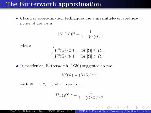
Classical approximation techniques use a magnitude-squared res-ponse of the form

|Hc(Ω)|2 =1

1 + V 2(Ω),

where V 2(Ω) 1, for |Ω| ≤ Ωc,

V 2(Ω) 1, for |Ω| > Ωc.

In particular, Butterworth (1930) suggested to use

V 2(Ω) = (Ω/Ωc)2N ,

with N = 1, 2, . . ., which results in

|HB(Ω)|2 =1

1 + (Ω/Ωc)2N.


The Butterworth approximation (cont.)

In this case, we have

|HB(Ω)|2 =

1, if Ω = 0,

1/2, if Ω = Ωc,

0, if Ω =∞.

Note that the transition approaches a “brick wall”, when N →∞.

Note also that |H(Ω)|2 is a monotone function of Ω.



The poles of HB(s)HB(−s) are found by solving

1 + (s/jΩc)2N = 0 ⇐⇒ (s/Ωc)

2N = −1 = e(2k−1)π,

with k = 1, 2, . . . , 2N .

The solution yields

sk = σk + Ωk = Ωc cos θk + Ωc sin θk,

where

θk =π

2+

2k − 1

2Nπ,

for k = 1, 2, . . . , 2N .

Thus, HB(s)HB(−s) has 2N poles, which are evenly distributedover a circle of radius Ωc in the complex plane.



A stable system function HB(s) can be formed by choosing the(first) N poles which lie in the left-half plane, resulting in

HB(s) =ΩNc

(s− s1)(s− s2) · · · (s− sN ).

Note that the numerator is equal to ΩNc to assure |HB( · 0)| = 1.


Design Procedure

Suppose we wish to design a Butterworth lowpass filter specifiedby parameters Ωp, Ωs, ε, and A.

Here 1/(1 + ε2) and 1/A2 define the passband and stopband rip-ple, respectively. Namely,

Ap = −10 log10

(1

1 + ε2

)and As = −10 log10

(1

A2

).

Using the relative specification, we then have

1

1 + (Ωp/Ωc)2N≥ 1

1 + ε2⇐⇒ (Ωp/Ωc)

2N ≤ ε2,

1

1 + (Ωs/Ωc)2N≤ 1

A2⇐⇒ (Ωs/Ωc)

2N ≥ A2 − 1.

The above inequalities can be combined to result in

ΩNp

√A2 − 1

ε≤ ΩNc

√A2 − 1 ≤ ΩNs .


Design Procedure (cont.)

Consequently, we obtain the following design equation.

Butterworth design equation

N =

⌈lnα

lnβ

⌉,

where

α ,ΩsΩp

, β ,

√A2 − 1

ε=

√10As/10 − 1√10Ap/10 − 1

.

The cut-off frequency Ωc can be chosen anywhere in the interval

Ωp(10Ap/10 − 1)−1/(2N) ≤ Ωc ≤ Ωs(10As/10 − 1)−1/(2N).

In MATLAB, Butterworth filters can be designed using

[N, Omegac] = buttord(Omegap, Omegas, Ap, As, ’s’)

[B, A] = butter(N, Omegac, ’s’)


Example

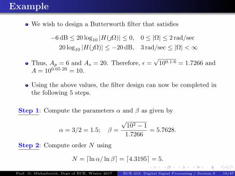
We wish to design a Butterworth filter that satisfies

−6 dB ≤ 20 log10 |H(Ω)| ≤ 0, 0 ≤ |Ω| ≤ 2 rad/sec

20 log10 |H(Ω)| ≤ −20 dB, 3 rad/sec ≤ |Ω| <∞

Thus, Ap = 6 and As = 20. Therefore, ε =√

100.1·6 = 1.7266 andA = 100.05·20 = 10.

Using the above values, the filter design can now be completed inthe following 5 steps.

Step 1: Compute the parameters α and β as given by

α = 3/2 = 1.5; β =

√102 − 1

1.7266= 5.7628.

Step 2: Compute order N using

N = dlnα/ lnβe = d4.3195e = 5.


Example

Step 3: Determine 3 dB cutoff frequency Ωc, whose lower and uppervalues are respectively given by

2(106/10 − 1)−1/10 = 1.7931 and 3(1020/10 − 1)−1/10 = 1.8948.

It seems reasonable to choose Ωc = 1.8948. (Why?)

Step 4: Compute pole locations.

sk = 1.8948 cos(0.4π + 0.2πk) + 1.8948 sin(0.4π + 0.2πk),

with k = 1, 2, 3, 4, 5.

Step 5: Compute the system function HB(s) as given by

HB(s) =5∏k=1

1.8948

s− sk=

24.42

s5 + 6.13s4 + 18.8s3 + 35.61s2 + 41.71s+ 24.42.


The Chebyshev approximation

The Chebyshev approximation results in equiripple design, whichis optimal with respect to the minimax optimization criterion.

The Chebyshev lowpass filter approximation is based on

|HC(Ω)|2 =1

1 + ε2T 2N (Ω/Ωc)

,

where TN is the N th order Chebyshev polynomial.


The Chebyshev approximation (cont.)

Formally, Chebyshev polynomials are defined as

TN (x) =

cos(N cos−1 x), |x| ≤ 1,

cosh(N cosh−1 x), |x| > 1.

Since the leading term of TN (x) is 2N−1xN , the values of T 2N (x)

grow very fast for |x| > 1.

Thus, in the stopband, we have T 2N (Ω/Ωc) 1 or, equivalently,

|HC(Ω)|2 1, for |Ω| > Ωc.

Moreover,

|HC( 0)|2 =

1, if N is odd,

1/(1 + ε2), if N is even,

and

|HC(Ωc)|2 =1

1 + ε2.



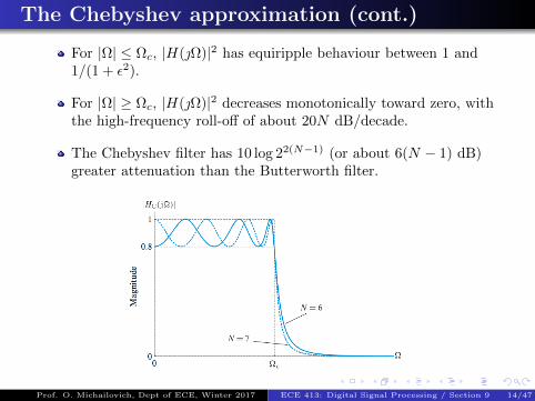
For |Ω| ≤ Ωc, |H(Ω)|2 has equiripple behaviour between 1 and1/(1 + ε2).

For |Ω| ≥ Ωc, |H(Ω)|2 decreases monotonically toward zero, withthe high-frequency roll-off of about 20N dB/decade.

The Chebyshev filter has 10 log 22(N−1) (or about 6(N − 1) dB)greater attenuation than the Butterworth filter.



The poles of HC(s)HC(−s) are obtained by solving

TN (s/Ωc) = ±ε.

Solving the equation yields

sk = σk + Ωk = (Ωc sinh(φ)) cos θk + (Ωc cosh(φ)) sin θk,

where

θk =π

2+

2k − 1

2Nπ, k = 1, 2, . . . , 2N,

andφ = (1/N) sinh−1 (1/ε) .

One can see that, as opposed to the case of Butterworth filters,the poles of Chebyshev filters are located on an elliptic curve.



To obtain a stable system, we assign to HC(s) the poles locatedon the left-half plane (σk < 0), which results in

HC(s) =G∏N

k=1(s− sk), with G =

N∏k=1

(−sk)×

1√

1+ε2, N even,

1, N odd.


Design procedure

Starting with the specified parameters Ωp, Ap, Ωs, and As, forequiripple response in the passband, we choose Ωc = Ωp.

Since |HC(Ωc)|2 = 1/(1 + ε2), the passband constraint is satis-fied for all 0 ≤ Ω ≤ Ωp.

In the stopband, we require that

1

1 + ε2T 2N (Ωs/Ωp)

≤ 1

A2⇐⇒ TN (Ωs/Ωp) ≥

√A2 − 1

ε.

Since Ωs/Ωp > 1, this inequality is equivalent to

cosh(N cosh−1(Ωs/Ωp)) ≥√A2 − 1

ε.


Design procedure (cont.)

Solving the above inequality produces the key design formulas.

Chebyshev I design equation

N ≥ cosh−1 β

cosh−1 α=

ln(β +√β2 − 1)

ln(α+√α2 − 1)

,

where

α =ΩsΩp

, β =

√A2 − 1

ε=

√10As/10 − 1√10Ap/10 − 1

.

In MATLAB, Chebyshev I filters can be designed using

[N, Omegac] = cheb1ord(Omegap, Omegas, Ap, As, ’s’)

[B, A] = cheby1(N, Ap, Omegac, ’s’)


Example

Once again, we design a filter that satisfies

−6 dB ≤ 20 log10 |H(Ω)| ≤ 0, 0 ≤ |Ω| ≤ 2 rad/sec

20 log10 |H(Ω)| ≤ −20 dB, 3 rad/sec ≤ |Ω| <∞

This time, however, we will use the Chebyshel I design.

As before, we have ε = 1.7266 and A = 10.

Step 1: Compute the parameters α and β as given by

α = 3/2 = 1.5; β =

√102 − 1

1.7266= 5.7628.

Step 2: Compute order N using

N =

⌈ln(5.7628 +

√5.76282 − 1

)ln(1.5 +

√1.52 − 1

) ⌉= d2.5321e = 3.


Example (cont.)

Step 3: Set Ωc = Ωp = 2, and compute

a = 2 · sinh((1/3) sinh−1(1/1.7266)

)= 0.3693,

b = 2 · cosh((1/3) sinh−1(1/1.7266)

)= 2.0338.

Step 4: Compute pole locations.

s1 = 0.3693 · cos(4π/6) + 2.0338 · sin(4π/6) = −0.1847− 1.7613,

s2 = 0.3693 · cos(6π/6) + 2.0338 · sin(6π/6) = −0.3693,

s3 = 0.3693 · cos(8π/6) + 2.0338 · sin(8π/6) = −0.1847 + 1.7613.

Step 5: Compute the filter gain G and the system function HC(s)

G = (0.1847 + 1.7613) · 0.3693 · (0.1847− 1.7613) · 1 = 1.1584.

HC(s) = 1.1584

3∏k=1

1

s− sk=

1.1584

s3 + 0.7387s2 + 3.2728s+ 1.1584.


Another example

Let us design a Chebyshev I filter with

Fp = 40 Hz, Ap = 1 dB,

Fs = 50 Hz, As = 30 dB.

using MATLAB.

To this end, we use the following script.

>> [N, Omegac] = cheb1ord(2*pi*40,2*pi*50,1,30,'s');

N =7

>> Fc = Omegac/(2*pi);

Fc =40

>> [B, A] = cheby1(N,Ap,Omegac,'s');


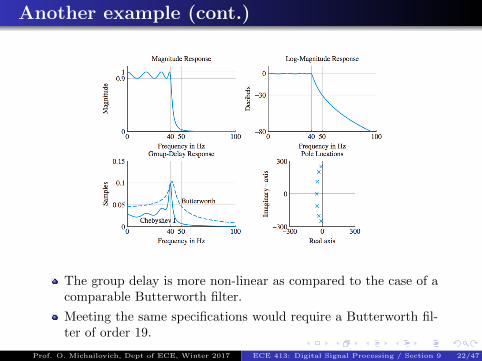
Another example (cont.)

The group delay is more non-linear as compared to the case of acomparable Butterworth filter.

Meeting the same specifications would require a Butterworth fil-ter of order 19.


The inverse Chebyshev approximation

Replacing the frequency variable Ω/Ωc by Ωc/Ω converts theChebyshev I low-pass filter into a Chebyshev highpass filter.

If we subtract the highpass characteristic from unity, we obtainthe inverse Chebyshev or Chebyshev II characteristic.

|HIC(Ω)|2 = 1− 1

1 + ε2T 2N (Ωc/Ω)

=ε2T 2

N (Ωc/Ω)

1 + ε2T 2N (Ωc/Ω)

.


The inverse Chebyshev approximation (cont.)

The Chebyshev II approximation exhibits equiripple behavior inthe stopband and monotonic maximally flat behavior in the pass-band.

This filter has both zeros and poles.

Specifically, the poles of the Chebyshev II filter are the reciprocalsof those of the Chebyshev I filter, viz.

sk =Ωc

σk/Ωc + Ωk/Ωc=

Ωcσk + Ωk

.

At the same time, the zeros of the Chebyshev II filter are

ξk = Ωc

cosuk, where uk =

2k − 1

2N

π

2, k = 1, 2, . . . , 2N.

Thus, the zeros and poles of the Chebyshev II filter do not lie onany simple geometric curve.


Example

The design of Chebyshev II filter is very similar to that of theChebyshev I filter.

In MATLAB, Chebyshev II filters can be built using

[N, Omegac] = cheb2ord(Omegap, Omegas, Ap, As, ’s’)

[B, A] = cheby2(N, As, Omegac, ’s’)


Continuous-to-discrete filter transformation

Our next step is to transform CT filters to their DT counterparts.

Each transformation is equivalent to a mapping function s = f(z)from the s-plane to the z-plane.

Any useful mapping should satisfy three desirable conditions:

1. A rational Hc(s) should be mapped to a rational H(z).2. The imaginary axis of the s-plane is mapped on the unit circleof the z-plane, viz.

s = Ω | Ω ∈ R 7→ z = eω | ω ∈ (π, π].

3. The left-half s-plane is mapped into the interior of the unitcircle of the z-plane, viz.

s | <s < 0 7→ z | |z| < 1.

Different procedures give rise to different mapping functions, and,hence, the resulting discrete-time filters are different.


Impulse-invariance transformation (IIT)

The most natural way to convert a CT filter to a DT filter is bysampling its impulse response

h[n] , Td hc(nTd), n ∈ Z.

This transformation is known as impulse-invariance transforma-tion (IIT), since it preserves the shape of the impulse response.

The resulting frequency response is

H(eω) =∑k

Hc

(ω

Td+

2π

Tdk

).

If the continuous-time filter is bandlimited, that is, Hc(Ω) = 0for |Ω| ≥ π/Td, then, we have

H(eω) = Hc(ω/Td), |ω| ≤ π.


Mapping for the IIT

What is the transformation s = f(z) in the case of IIT?

To answer this question, we start with a system function

Hc(s) =

N∑k=1

Aks− sk

,

where the poles are assumed to be distinct.

Taking the inverse Laplace transform yields

hc(t) =

N∑k=1

Akesktu(t).

Thus, the impulse response of the discrete-time filter is given by

h[n] =

N∑k=1

Ak(Tde

skTdn)u[n] = Td

N∑k=1

Ak(eskTd

)nu[n].


Mapping for the IIT (cont.)

The resulting system function of the discrete-time system istherefore given by

H(z) =∑n

h[n]z−n =

∞∑n=0

N∑k=1

TdAk(eskTd

)nz−n.

Interchanging the orders of summations yields

H(z) =

N∑k=1

TdAk1− eskTdz−1

,

where we assumed that |eskTd | < 1.

Thus, we have a transformation of the form

1

s− sk→ Td

1− pkz−1, with pk = eskTd .



Note that the transformation

1

s− sk=⇒ Td

1− pkz−1

maps the poles of the continuous-time filter to the poles of itsdiscrete-time counterpart.

Therefore, the mapping s = f(z) corresponding to impulse inva-riance is defined by z = esTd .

More specifically, since s = σ + Ω, we have

r = eσ Td and ω = ΩTd.

Note that σ < 0 implies 0 < r < 1, while σ > 0 implies r > 1.

Since σ = 0 yields r = 1, the imaginary axis s = Ω is mappedonto the UC. This map, however, is not one-to-one due to theeffect of aliasing.



Due to periodicity in ω, each horizontal “strip” of height 2π/Tdin the s-plane is mapped into the entire z-pane.

In fact, we have

H(z)∣∣∣z=esTd

=

∞∑k=−∞

Hc

(s+

2πk

Td

).


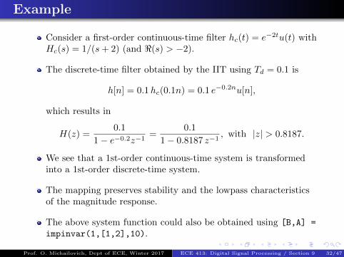
Example

Consider a first-order continuous-time filter hc(t) = e−2tu(t) withHc(s) = 1/(s+ 2) (and <(s) > −2).

The discrete-time filter obtained by the IIT using Td = 0.1 is

h[n] = 0.1hc(0.1n) = 0.1 e−0.2nu[n],

which results in

H(z) =0.1

1− e−0.2z−1=

0.1

1− 0.8187 z−1, with |z| > 0.8187.

We see that a 1st-order continuous-time system is transformedinto a 1st-order discrete-time system.

The mapping preserves stability and the lowpass characteristicsof the magnitude response.

The above system function could also be obtained using [B,A] =

impinvar(1,[1,2],10).


Limitations of the IIT

Consider the high-pass filter obtained by Hc(s) = 1−Hc(s) == 1− 1/(s+ 2) = (s+ 1)/(s+ 2).

The impulse response of the high-pass filter is

hc(t) = δ(t)− hc(t) = δ(t)− e−2tu(t).

The presence of δ(t) renders the IIT approach impractical.

Since the delta function appears when N = M , the IIT cannot beused for systems with improper system functions (like high-pass &band-stop filters).

Impulse-invariance can be applied to low-pass & band-pass filtersthat have strictly proper transfer functions.


Design procedure

Starting with the design parameters ωp, ωs, Ap and As, firstcompute Ωp = ωp/Td and Ωs = ωs/Td for some Td.

Subsequently, design an equivalent continuos-time filter (such as,e.g., Butterworth or Chebyshev I).

Finally, map the “continuous poles” into the ”discrete poles” ac-cording to

pk = eskTd , ∀k,

to result in H(z).

We note that the above design does not depend on a particularvalue of Td, which therefore may be set arbitrarily.


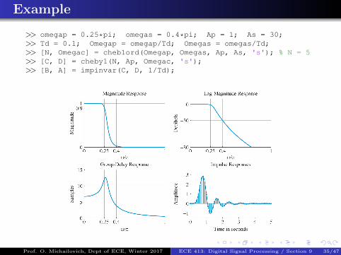
Example

>> omegap = 0.25*pi; omegas = 0.4*pi; Ap = 1; As = 30;>> Td = 0.1; Omegap = omegap/Td; Omegas = omegas/Td;>> [N, Omegac] = cheb1ord(Omegap, Omegas, Ap, As, 's'); % N = 5>> [C, D] = cheby1(N, Ap, Omegac, 's');>> [B, A] = impinvar(C, D, 1/Td);


Bilinear transformation

To avoid the aliasing-related problems of the IIT, a one-to-onemapping from the s-plane to the z-plane is required.

One of such mapping is the bilinear transformation given by

s = f(z) =2

Td

1− z−1

1 + z−1.

Here, Td is not interpreted as a sampling interval, and can havean arbitrary value.

Given Hc(s), the bilinear transform is applied as

H(z) = Hc(s)∣∣∣s= 2

Td

1−z−1

1+z−1

.

In this case, every zero/pole νk is transformed according to

s− νk =2(1− Tdνk/2)

Td(1 + z−1)

[1− 1 + Tdνk/2

1− Tdνk/2z−1

].


Bilinear transformation (cont.)

One can show that the mapping results in

H(z) = G(1 + z−1)N−M

∏Mk=1(1− zkz−1)∏N

k=1(1− pkz−1),

where

zk =1 + Tdξk/2

1− Tdξk/2, pk =

1 + Tdsk/2

1− Tdsk/2,

and

G =β0(Td/2)N−M

∏Mk=1(1− ξkTd/2)∏N

k=1(1− skTd/2),

where β0 is the gain of the CT filter.

In MATLAB, the above transformations are implemented byfunctions

[zd, pd, G] = bilinear(zc, pc, beta0, Fd)

[B, A] = bilinear(C, D, Fd)


Example

Consider the following CT system:

Hc(s) =5(s+ 2)

(s+ 3)(s+ 4)=

5s+ 10

s2 + 7s+ 12.

In this case, we obtain (using Td/2 = 1)

z1 =1 + (−2)

1− (−2)= −1

3, z2 = −1,

p1 =1 + (−3)

1− (−3)= −1

2,

1 + (−4)

1− (−4)= −3

5,

as well as

G =5 · 1 · (1− (−2))

(1− (−3))(1− (−4))=

3

4.

Hence,

H(z) =3

4

(1 + z−1)(1 + 1/3z−1)

(1 + 1/2z−1)(1 + 3/5z−1)=

0.75 + z−1 + 0.25z−2

1 + 1.1z−1 + 0.3z−2.


Mapping properties

In terms of the s variable, we have

z = reω =2/Td + s

2/Td − s=

2/Td + σ + Ω

2/Td − σ − Ω.

One can then show that: 1) r < 1 if σ < 0, 2) r = 1 if σ = 0, and3) r > 1 if σ > 0.

Thus, the bilinear transformation preserves stability.

At the same time, ω and Ω are related as

ω = 2 tan−1(ΩTd/2) or Ω = (2/Td) tan(ω/2),

which shows that

Ω = 0 ⇒ ω = 0

Ω =∞ ⇒ ω = π

Ω = −∞ ⇒ ω = −π.


Mapping properties (cont.)

Therefore, we have the following type of mapping.

Since the entire Ω axis is mapped onto the UC, the transforma-tion is free of aliasing artifacts.

However, the highly nonlinear relation between Ω and ω needs tobe treated with precaution.


Frequency warping

The nonlinear relation between Ω and ω is known as frequencywarping.

The relation is approximately linear for |ω| ≤ 0.3π. Thus, anyshape of magnitude response in this range is preserved.

Frequency warping does not distort “flat” magnitude responses.

Frequency warping distorts “non-flat” magnitude responses. (So,a CT differentiator cannot be converted to a DT one.)


Frequency warping (cont.)

Frequency warping distors the location of frequency bands andtheir width.

Therefore, the design specifications for the CT filter have to bedetermined by prewarping according to

Ωk =2

Tdtan

ωk2,

where ωk is a required band edge.

During the bilinear transformation, the frequencies are properly“unwarped”, in which case the effect of Td is cancelled.

In practice, it is often convenient to use Td = 2.

In summary, the use of bilinear transformation should be avoidedwhen designing wideband discrete-time differentiators and linear-phase filters.


Frequency warping (cont.)


Design procedure

Starting with the design parameters ωp, ωs, Ap and As, first setTd = 2 and compute Ωp = tan(ωp/2) and Ωs = tan(ωs/2).

Subsequently, design an equivalent continuos-time filter (such as,e.g., Butterworth, Chebyshev I, or Chebyshev II) Hc(s).

Determine zeros, poles, and gain of Hc(s) and map these quanti-ties into corresponding zeros, poles, and gain of H(z).

Finally, assemble the desired digital filter system function H(z).

Note that all the above procedures are performed by MATLABfunction bilinear.


Frequency transformations of low-pass filters

Frequency transformations are needed to transform low-pass fil-ters to high-pass, band-pass, and band-stop filters.

Given a prototype CT low-pass filter Hc(s) and its discrete coun-terpart H(z), one can apply frequency transformation to eitherHc(s) (continuous) or H(z) (discrete).

If the bilinear transformation is used to convert Hc(s) into H(z),the frequency transformation can be applied to either of the two.

If the IIT is used instead, the frequency transformation should beapplied to H(z). (Why?)


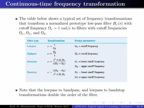
Continuous-time frequency transformation

The table below shows a typical set of frequency transformationsthat transform a normalized prototype low-pass filter Hc(s) withcutoff frequency Ωc = 1 rad/s to filters with cutoff frequenciesΩc, Ω1, and Ω2.

Note that the lowpass to bandpass, and lowpass to bandstoptransformations double the order of the filter.


Discrete-time frequency transformation

Discrete-time frequency transformations are usually performedthrough z−1 7→ G(z−1), where

G(z−1) = ±N∏k=1

z−1 − α∗k1− αkz−1

,

with |αk| < 1.

By properly choosing the values of N and αk, one can obtain avariety of mappings.

For specific formulas, see p.678 of the course textbook.

In MATLAB, frequency transformations are performed by func-tions lp2lp, lp2hp, lp2bp, and lp2bs.

The FDATool of MATLAB provides a convenient environmentfor designing a variety of different digital filters.


Documents

Design of IIR lters - University of Waterlooece413/Sections/section9.pdf · Design of IIR lters ... 10 jH(|)j 0; 0 j j 2rad=sec 20log ... (8ˇ=6) = 0:1847 + |1:7613: Step 5: Compute