Embed Size (px)
Citation preview

Design of Headworks in steep sediment loaded riversA model study case of Lower Manang
Marsyangdi Hydropower Project
Abha Dudhraj
Civil and Environmental Engineering
Supervisor: Leif Lia, IVMCo-supervisor: Hanne Nøvik, IVM
Department of Hydraulic and Environmental Engineering
Submission date: June 2013
Norwegian University of Science and Technology


NTNU Fakultet for ingeniørvitenskap Norges teknisk-naturvitenskapelige og teknologi Universitet Institutt for vann- og miljøteknikk
MASTER THESIS SPRING 2013
Student: Abha Dudhraj
Title: DESIGN OF HEADWORKS IN STEEP SEDIMENT LOADED
RIVERS – A MODEL STUDY CASE OF LOWER MANANG
MARSYANGDI Hydropower Project
Tittel: UTFORMING AV INNTAK I BRATTE, SEDIMENTFØRENDE
ELVER – MODELSTUDIE AV LOWER MANANG
MARSYANGDI VANNKRAFTVERK
1 INTRODUCTION A well-functioning intake is a prerequisite for the successful operation of a
hydropower plant. The main challenges with developing good design principles
for shallow intakes for hydropower plants involve sediment handling, floating
debris, leaves, ice, entrainment of air and general hydraulic conditions. It is a
major challenge to meet all these sometimes-incompatible requirements in the
design of an intake in a shallow river with rapid flow. Internationally, and
specifically in the Himalayas, with a heavy rainy season combined with a lot of
sediments, sediment handling is the major concern. Settling basins are common
components at headwork for minimizing sediment erosion of the waterways
and the turbines. Therefore, a headwork design adapted to local conditions is
essential. There are various principles for the design of intakes existing today;

some are more successful than others. Several intake structures undergo
reconstruction or modification after only a few years in service, due to
problems with maintenance and operation due to a design poorly adapted to
local conditions.
Both private initiatives and hydropower companies are contributing with new
solutions through model testing of headwork in the hydraulic laboratories.
Hydro Lab Pvt. Ltd., Kathmandu and NTNU Vassdragslaboratoriet, Trondheim
seeks to contribute to further development, verification and innovation within
this area.
2 BACKGROUND Sediment handling in steep sediment loaded rivers normally requires settling
basins. Flushing of settling basins and sand traps is widely used, and different
flushing concepts have been developed. Because of the unique conditions for
every single hydropower project and the complexity of the sediment transport,
physical and/or numerical model studies of the headwork are often
recommended. Experiences from existing hydropower plants and available
physical models are very valuable tools for planning and design of new
headwork. A physical model of the headwork of the 138 MW Lower Manang
Marsyangdi Hydropower Project (LMM HPP), located in Manang District of
Gandaki Zone in Nepal, is built at Hydro Lab Pvt. Ltd. in Kathmandu, Nepal. The
plant is scheduled to be commenced by 2017.
3 PROBLEM DESCRIPTION Theory of headwork design in general, and sediment handling especially, in
addition to experiences from case studies from hydro power plants already
built must be studied. A test program shall be designed for a model study of the
headwork of the LMM HPP. The goal of the physical model study of the LMM
HPP conducted at Hydro Lab Pvt. Ltd. is to evaluate the given design and
improve the performance of the headwork especially with respect to sediment
handling arrangement, both during normal conditions and during floods.
Modified intake arrangement should be tested for normal monsoon flow and
flows higher than this. The tests should include study of flow patterns in the
intake area and the settling basins; bed control in front of the intake and
passage of floating debris. Specific aspects of the headwork hydraulics should

be assessed by a numerical model study, and compared to observations from
the physical model. All the tests should be documented and reported.
4 GOAL The overall goal of the master thesis is to gain experiences on intake hydraulics
and headwork design. Theoretical aspects of headwork design must be
implemented during the assessment of the performance of the LMM
headwork. Uncertainties and errors should be evaluated. It should be
concluded on whether the work has been successful or if there should be
further studies needed to be conducted.
5 CONTACT PERSONS
NTNU Leif Lia, Professor (supervisor)
Hanne Nøvik, PhD-student (co-supervisor)
Hydro Lab Ltd Durga P. Sangroula
Usha Shrestra
Butwal Power Company (BPC) Pratik Man Sing Pradhan
Discussions with colleagues and employees at NTNU, SINTEF, Hydro Lab, BPC
and eventually other hydro power plants are recommended. All contributions
should be correctly referred.
6 REPORT FORMAT, REFERENCES AND CONTRACT The report should be written with a text editing software, and figures, tables,
photos etc should be of good quality. The report should contain an executive
summary, a table of content, a list of figures and tables, a list of references and
information about other relevant sources. The report should be submitted
electronically in B5-format .pdf-file in DAIM, and three paper copies should be
handed in to the institute.
The executive summary should not exceed 450 words, and should be suitable
for electronic reporting.
The Master’s thesis should be submitted within Monday 10th of June 2013.


i
Abstract
Headworks design in steep, sediment loaded rivers is challenging. Technical
challenges related to the functionalities of the headworks area have been
studied for the case of Lower Manang Marsyangdi (LMM) Hydropower Project
(HPP), which is under design phase in Nepal. The Physical Hydraulic Model
(PHM) study conducted at Hydro Lab focuses on intake hydraulics, sediment
handling and trash removal along the intake. Experience from the physical
model study of the LMM headworks has shown that the passage of sediments
and bed control during flood periods are the major challenges in this
hydropower project. Design of an optimal bed load handling component and
the settling basin are very important to handle sediments without affecting the
regularity in power generation.
Velocity measurements were conducted at several cross-sections along the
settling basins to evaluate the hydraulics. Turbulent Kinetic Energy (TKE) was
calculated from the velocity measurements to assess the effect of secondary
currents. The study has further focused on the concept of numerical modeling
to replicate the hydraulics in the existing headworks model of LMM HPP. A
Three-dimensional (3D) CFD-program, STAR CCM+, has been used to conduct
the numerical model study of the intake hydraulics of LMM headworks.
Through dye tests and measurements on the PHM it has been shown that final
conceptual design, which is based on modifications conducted on the initial
design, has an improved hydraulics along the intake. Vortices/eddies in front of
the intakes and along the settling basins have been reduced and a uniform,
symmetrical flow with the desired velocity of less than 1.00 m/s prototype
value has been achieved along the settling basins. Further evaluation of TKE has
shown significant decrease of turbulence level along the settling basins.
Use of numerical model has to a large extent been successfully able to replicate
the hydraulics in the modeled headworks of LMM HPP. The velocity range is
comparable to the measured values in the laboratory. However, secondary
currents and, thereby, the TKE values have not been reproduced properly in the
numerical model. TKE for the first cross-section close to the inlet of the basin is

ii
similar but no significant trend can be observed between the other cross-
sections.
Numerical model requires boundary conditions determined from the PHM and
results need to be validated against laboratory measurements to ensure their
accuracy. Thus, it is recommended for numerical model studies to be used in
combinations with PHM study. Numerical model requires an initial validation by
comparing simulated flows to measured flows from the laboratory. The
validated numerical model can then be used to predict further effects of
modification in the headworks design and to optimize the conceptual design.
iii
Sammendrag
Basert på resultatene fra det fysiske modellstudiet har det blitt konkludert med
at utforming av inntak i bratte, sedimentførende elver er spesielt
utfordrende.Tekniske utfordringer knyttet til inntaksområdet har blitt vurdert
for Lower Manang Marsyangdi (LMM) vannkraft prosjekt i Nepal.
Inntakhydraulikken i tillegg til håndtering av sediment og drivgods langs
inntaket har blitt fokusert på i det fysiske modellstuidet gjennomført i
samarbeid med Hydro Lab.
Hastighetsmålinger ble utført langs flere tverrsnitt langs
sedimenteringsbassengene i den fysiske modellen for å evaluere
strømningsforholdene. Turbulent Kinetisk Energi (TKE) ble beregnet fra
hastighetsmålinger for å vurdere effekten av sekundære strømninger i
bassengene. Videre er det brukt numerisk modellering for å gjenskape
hydraulikken langs inntaksområdet i den fysiske modellen av LMM. Den
tredimensjonale (3D) CFD-program, STAR CCM +, har blitt brukt til å utføre
denne simuleringen.
Forbislipping av sedimenter og kontroll av bunnivå ved inntaket, spesielt for
flomperioder, er de største utfordringene i dette vannkraftsprosjektet.
Utformingen av en velfungerende bunnspyleluke og sedimenteringsbassenget
er svært viktig for å kunne håndtere sedimenter uten å ha for store
innvirkninger på kraftverksproduksjonen.
Ved bruk av markørvæske har det blitt utført tester og målinger i den fysiske
modellen. Den endelige utformingen av inntaksområdet, som er basert på
modifikasjoner av den opprinnelige utformingen, har en klar forbedret
hydraulikk langs inntaket. Virveldannelser foran inntaksåpningene og langs
sedmenteringsbassengene er redusert, og en jevn og symmetrisk strømning
med hastighet på mindre enn 1.00 m/s i prototyp verdi, er oppnådd langs
bassengene. Videre evaluering av TKE har vist betydelig reduksjon av
turbulensnivå langs med sedimenterings bassengene.
Bruk av den numeriske modellen har i stor grad vært vellykket og er i stand til å
gjenskape inntakshydraulikken i den fysiske modellen av LMM. Hastighetene er

iv
sammenlignbare med de målte verdiene i laboratoriet. Derimot, har ikke den
numeriske modellen klart å gjenskape sekundære strømningene og TKE verdier
fra den fysiske modellen. TKE for det første tverrsnittet som er i nærheten av
innløpet til sedimenteringsbassengene samsvarer bra med de målte verdiene,
men for de andre tversnittene derimot, er det ingen tydelig samsvar mellom de
målte og simulerte verdiene.
Numeriske modeller krever grensebetingelser som kan bestemmes fra målte
verdier fra fysiske modeller og resultatene må vurderes opp mot
laboratoriemålinger for å verifisere nøyaktighet i resultatene fra simuleringene.
Således er det anbefalt å bruke et numeriske modellstudie i kombinasjon med
et fysisk modellstudie. Resultatene fra numeriske modeller må kontrolleres ved
å sammenligne de mot målte verdier fra laboratoriet/felt. Deretter kan den
numeriske modellen brukes for å forutsi ytterligere effekter ved endringer i
utforming av ulike inntakskomponenter og for å optimalisere modellen frem til
den endelige design.
v
Preface
This report is developed as an output of the Master’s thesis conducted under
the guidance and co-operation of the Institute of Hydraulics and Environmental
Engineering.
The thesis is a combination of a Physical Hydraulic Model study and a
Numerical Hydraulic Model study conducted on the headworks of Lower
Manang Marsyangdi Hydropower project under design in Nepal.
The study has increased my understanding on intake hydraulics and sediment-
related problems in hydropower plants with steep, sediment-loaded rivers. The
thesis has also given me the opportunity to learn a new software program, Star
CCM+, its applications and the use of numerical model as a tool in the
verification and understanding of river hydraulics.
I would first and foremost, like to extend my gratitude to my supervisor Leif Lia
for the necessary support provided for the development of this thesis.
Furthermore, I would like to sincerely thank my co-supervisor Hanne Nøvik who
has constantly encouraged me and provided continuous supervision to aid the
writing of this thesis. Guidance from Torgeir Jensen, SINTEF, on the usage of
ADV measurements in the laboratory is deeply appreciated. Similarly, the
suggestions and assistance provided by the staff at Hydro Lab Pvt. Ltd. during
my stay in Nepal is immensely valued. Last but not the least; I am very grateful
to my friends and family for the adequate moral support during this period.

vi
vii
Table of Contents
1 Introduction .................................................................................................. 1
2 Background ................................................................................................... 3
2.1 The Lower Manang Marsyangdi HPP ................................................... 3
2.2 Challenges in LMM HPP ........................................................................ 5
3 Theoretical background ................................................................................ 9
3.1 Design of headworks in steep sediment loaded rivers ........................ 9
3.1.1 Performance standards .............................................................. 10
3.1.2 Intake hydraulics ........................................................................ 13
3.1.3 Settling Basin Design .................................................................. 15
3.2 Model theory ...................................................................................... 18
3.3 Numerical Modeling – CFD ................................................................. 20
3.3.1 Grids ........................................................................................... 20
3.3.2 Navier Stokes equations ............................................................. 20
3.3.3 Discretization methods .............................................................. 21
3.3.4 Turbulence models ..................................................................... 22
3.3.5 Stability and convergence .......................................................... 23
3.3.6 Courant Number ......................................................................... 24
4 Methodology .............................................................................................. 25
5 Physical hydraulic model study of the headworks of LMM HPP ................ 27
5.1 Model study methodology ................................................................. 27
5.2 The initial design................................................................................. 28
5.3 Analysis of the initial design against the Final arrangement.............. 30
5.3.1 Intake Hydraulics ........................................................................ 30
6 Velocity measurements on the Physical Hydraulic Model of LMM HPP .... 39
6.1.1 Acoustic Dopple Velocity Meter (ADV) ...................................... 39
6.2 Procedure for the ADV measurements .............................................. 40

viii
6.3 Micro propeller measurements ......................................................... 42
7 Numerical model study of the headworks of LMM HPP ............................ 45
7.1 Star CCM+ ........................................................................................... 45
7.2 The numerical model setup ................................................................ 45
7.2.1 Pre-processing ............................................................................ 45
7.2.2 Post processing ........................................................................... 55
8 Results ........................................................................................................ 57
8.1 Results from the numerical simulation .............................................. 57
8.1.1 Reliability and convergence of the numerical simulation .......... 57
8.1.2 Streamlines ................................................................................. 58
8.1.3 Pressure ...................................................................................... 59
8.1.4 Velocity distribution ................................................................... 60
8.1.5 Turbulent kinetic energy (TKE) ................................................... 60
8.1.6 Vorticity ...................................................................................... 61
8.2 Results from measurements in the physical model ........................... 61
8.2.1 Velocity measurements along the intake ................................... 61
8.2.2 Velocity measurements along the gravel trap ........................... 62
8.2.3 Comparison of measurements and simulations ......................... 63
8.3 Vorticity in the numerical simulation ................................................. 70
9 Discussion ................................................................................................... 73
9.1 Physical Hydraulic Model studies of Headworks ................................ 73
9.2 Measurements on the Physical Hydraulic Model ............................... 75
9.3 Comparison of simulated results and measurements ....................... 76
10 Conclusion .............................................................................................. 79
11 Further work and Recommendations .................................................... 81
Bibliography ........................................................................................................ 83
Appendix A Case studies of headworks design of physical hydraulic models
(PHM) ................................................................................................................. 85

ix
Kabeli A HPP ................................................................................................... 85
Initial arrangement vs the Final arrangement ............................................ 86
Khudi HPP ....................................................................................................... 93
The initial arrangement .............................................................................. 94
Modifications adopted for the final arrangement ..................................... 95
Effects and Evaluation of the modifications ............................................... 98
Appendix B Salient features for the initial headworks design of LMM HPP .... 101
Appendix C Velocity distributions along various Cross-Sections (CS) .............. 103
12 Appendix D Plan layout of the final design of LMM ............................. 105

x

xi
List of figures
Figure 1 Location of LMM (source: googlemaps) ................................................. 3
Figure 2 Initial PHM LMM (Shrestha and Bogati, 2012) ....................................... 4
Figure 3 Upstream river conditions of the headworks site of LMM (Nielsen and
Rettedal, 2012) ..................................................................................................... 5
Figure 4 Sediment transportation rates LMM (Shrestha and Bogati, 2012) ........ 6
Figure 5 Flow Duration Curve LMM HPP (Shrestha and Bogati, 2012) ............... 7
Figure 6 PSD for flow up to Average Monsoon Flow LMM HPP (Shrestha and
Bogati, 2012) ........................................................................................................ 7
Figure 7 Major headworks components (Jennsen et al., 2006) ........................... 9
Figure 8 Turbulent flow fields near the intake(Jennsen et al., 2006) ................ 10
Figure 9 Spillway at Middle Marsyangdi HPP ..................................................... 11
Figure 10 Intake cloggage at Khudi HPP(Shrestha et al., 2008) ........................ 12
Figure 11 Undersluice slots at Middle Marsyangdi HPP (Nielsen and Rettedal,
2012)................................................................................................................... 12
Figure 12 Turbulent flow regimes (Oslen, 2011) ................................................ 14
Figure 13 Sediment deposition in the settling basins of Khudi HPP .................. 15
Figure 14 General layout of settling basin (Lysne et al., 2003) ......................... 17
Figure 15 Flow tranquilizers at the inlet of ........................................................ 17
Figure 16 Different type of grid structures (Hasaas, 2012) ................................ 20
Figure 17 Comparison of the model and prototype of the headworks site of
LMM HPP (Shrestha and Bogati, 2012) .............................................................. 28
Figure 18 Initial physical model of the headworks of LMM HPP (Shrestha and
Bogati, 2012) ...................................................................................................... 29
Figure 19 Final arrangement of the intake of the PHM of LMM HEP ................ 30
Figure 20 Problems downstream on the inital arrangenement of the PHM of
LMM HPP (Shrestha and Bogati, 2012) .............................................................. 31
Figure 21 Initial design of the bed load hopper ................................................. 32
Figure 22 Bed control at the initial arrangement of LMM HPP (Shrestha and
Bogati, 2012) ...................................................................................................... 33
Figure 24 Settling basin inlet in the initial arrangement of LMM HPP (Shrestha
and Bogati, 2012) ............................................................................................... 34
Figure 23 Bed Control at the final arrangement of LMM HPP ........................... 34
Figure 25 Settling basin outlet in the initial arrangement of LMM HPP ............ 35
Figure 26 Final arrangement of the SB of LMM HPP .......................................... 35
xii
Figure 27 Final arrangement of the approach canals in the PHM of LMM HPP 36
Figure 28 Final arrangement on theSettling Basin outlet in the PHM of LMM
HPP ..................................................................................................................... 36
Figure 29 Final arrangement of the PHM of LMM HPP ...................................... 37
Figure 30 Standard ADV Field Probe ................................................................. 39
Figure 31 Side looking 3D probe ........................................................................ 40
Figure 32 ADV measurements along the settling basins of the PHM of LMM HPP
............................................................................................................................ 40
Figure 33 Measured Cross-sections along the Settling Basins of LMM HPP ...... 41
Figure 34 ADV measurements at the intake orifice of LMM HPP ...................... 42
Figure 35 Mini Air 20 Micropropeller ................................................................. 42
Figure 36 MicroPropeller measurements at the intake of the PHM of LMM HPP
............................................................................................................................ 43
Figure 37 Imported geometry from AutoCAD; x-direction shows the direction of
flow ..................................................................................................................... 46
Figure 38 Surface parts in the NHM ................................................................... 47
Figure 39 Surface diagnostics of the NHM ......................................................... 47
Figure 40 Volume mesh at the intake ................................................................ 49
Figure 41 Derived parts in the NHM................................................................... 53
Figure 42 Residual plot of the numerical simulation ......................................... 57
Figure 43 Mass flow plot of the numerical model ............................................. 58
Figure 44 Streamlines of the numerical model .................................................. 59
Figure 45 Pressure development in the numerical model ................................. 59
Figure 46 Velocity distributions along a plane section in the numerical model 60
Figure 48 Vorticity along the settling basin ........................................................ 61
Figure 47 Distribution of turbulent kinetic energy in the model ....................... 61
Figure 49 Velocity measurements along the intake ........................................... 62
Figure 50 Velocity measurements along the gravel trap ................................... 63
Figure 51 Comparison of velocity field close to the bottom of the settling basin
............................................................................................................................ 64
Figure 52 Comparison of velocity field along the middle plane section of the
settling basin ...................................................................................................... 64
Figure 53 Comparison of velocity field close to the surface of the settling basin
............................................................................................................................ 64
Figure 54 Velocity field settling basin LMM ,Cross-section 2 ............................. 66
Figure 55 Comparison of TKE development along the settling basin ................ 67

xiii
Figure 56 TKE along the settling basin ............................................................... 68
Figure 57 TKE at Cross-section 4 ........................................................................ 68
Figure 58 Velocity along the gravel trap ............................................................ 69
Figure 59 TKE based on ADV measurements along the gravel trap ................... 69
Figure 60 Simulation of vorticity along the settling basin .................................. 70
Figure 61 Simulated vorticity at various depths ................................................. 71
Figure 62 Headworks site of Kabeli'A' HPP(Bogati, 2012) .................................. 85
Figure 63 Kabeli A Headworks of the initial design (Bogati, 2012) .................... 86
Figure 64 Initial (Left) vs Final (right) intake design Kabeli 'A' ........................... 87
Figure 65 Initial design of the stilling Basin at Kabeli'A' HPP(Bogati, 2012) ....... 88
Figure 66 Final design of the stilling basin at Kabeli 'A' HPP .............................. 88
Figure 67 Final design of the approach tunnels for the PHM of kabeli 'A' HPP 91
Figure 68 Final design settling basin Kabeli 'A' HPP ........................................... 91
Figure 69 Modifications at the approach tunnel and inlet transition of the
settling basin(Bogati, 2012) ................................................................................ 92
Figure 70 Final arrangement Kabeli 'A' HPP ....................................................... 92
Figure 71 Headworks site of Khudi HPP (Shrestha et al., 2008) ......................... 93
Figure 72 PHM of the headworks of Khud HPP (Shrestha et al., 2008) ............. 94
Figure 73 Modifications at the intake of PHM of Khudi HPP (Shrestha et al.,
2008)................................................................................................................... 96
Figure 74 Modifications along the gravel trap on the PHM of Khudi HPP
(Shrestha et al., 2008) ........................................................................................ 97
Figure 75 Modifications at the downstream river slope of Khudi HPP (Shrestha
et al., 2008) ......................................................................................................... 97
Figure 76 River training structures Khudi model (Shrestha et al., 2008) ........... 97
Figure 77 River training structures at the intake of PHM of Khudi HPP (Shrestha
et al., 2008) ......................................................................................................... 98
Figure 78 Final arrangement of the PHM of Khudi HPP ..................................... 98

xiv
List of tables
Table 1 Flow discharge LMM (Shrestha and Bogati, 2012) .................................. 6
Table 2 Classification of the flushing systems .................................................... 13
Table 3 Scale ratios for various parameters when using the Froude model law
(Lysne, 1982) ...................................................................................................... 19
Table 4 Measured Cross-sections along the Settling Basins of LMM HPP ......... 41
Table 5 Overview of the selected mesh models ................................................ 48
Table 6 Overview on the selected physics model .............................................. 51
Table 7 Selected boundary conditions ............................................................... 54
Table 8 Under-relaxation factors used in the numerical model ........................ 55

xv
List of Symbols
Symbol Definition
LMM
HPP
ROR
CFD
BPC
DoED
m/s
m3/s
Mm3
SB
CS
ADV
3-D
S4
DNS
LES
RANS
TKE/k
δij
νT
ω
ε
STL
VOF
Fr
Q
t
MW
GWh
m
Re
D
L
u
ν
ρ
masl
Lower Manang Marsyangdi
Hydropower Project
Run-of-River scheme
Computational fluid mechanics
Butwal Power Company
Department of Electricity Development
Metre per second
Cubic metre per second
Million cubic metre
Settling Basin
Cross-section
Acoustic Doppler Velocimeter
Three dimensional
Serpent Sediment Sluicing System
Direct Numerical simulation
Large Eddy Simulation
Reynolds Averaged Navier Stokes Equations
Turbulent kinetic energy
Kronecker delta
Eddy viscosity
Specific dissipation rate
Dissipation of Turbulent kinetic energy
Stereo Lithography
Volume of fluid
Froude number
Discharge
Time
Mega Watt
Giga Watt hour
metre
Reynolds number
Diameter
Length
velocity
Kinematic viscosity
Density
metre above sea level

xvi

1
1 Introduction
Steep rivers mounting from the glaciers in the Himalayas along with varying
topography and heavy monsoon periods provide Nepal with a huge potential
for hydropower development. Consequently, with nearly 86% of the electricity
supply from hydropower (Nai, 2004) Nepal is heavily reliant on water
resources. The total estimated hydropower potential is 83 000MW out of which
43 000MW is deemed technically and economically viable for development.
However, due to the social and economical complications in the country the
total installed capacity amounts to 705 MW (Shrestha, 2012). Furthermore,
according to a world bank study about 63% of the Nepalese households lack
access to electricity (Banerjee et al., 2011). The deficiency in electricity is
therefore creating an enormous need for development in the hydropower
sector in the years ahead.
A functional intake is a prerequisite to ensure successful operation of both the
existing and new Hydropower Projects (HPP) that are under development.
Proper conceptual planning and design of the headworks is therefore required
for the further development of HPP in the country. Technical challenges related
to the headworks area have been studied for the case of Lower Manang
Marsyangdi (LMM) HPP in further detail in the following chapters. Intake
hydraulics along with sediment handling and trash removal has especially been
focused.
Lower Manang Marsyangdi Hydropower Project (LMM HPP) located in the
Gandaki zone in western Nepal has been studied and designed for development
by Hydro Consult Engineering Limited (Ltd.) for Butwal Power Company (BPC).
Physical model study of the headworks area is being conducted at Hydro Lab
Private Limited (Pvt. Ltd.), hydraulic laboratory in Nepal in order to assess the
overall performance of the headworks design in terms of its functionality.
A field trip to Nepal was conducted during the course of this thesis in order to
use existing theories and experiences from previous physical model studies
conducted in Hydro Lab to evaluate the intake hydraulics and headwork design
of LMM HPP. In order to gain experience from previous physical model studies
two case studies have been conducted based on reports prepared by Hydro Lab
during the two months stay in Nepal. The first case study presented is the

2
performance assessment of the headworks of Kabeli ‘A’ HPP designed and
studied for development. The second case is the study of existing headworks of
Khudi HPP, which had been suffering from intake clogging already during the
plants first year of operation. The two case studies mentioned are presented in
Appendix A.
The design of LMM HPP as provided by Hydro Consult has been evaluated and
compared with the design improvements suggested by Hydro Lab for the final
design. Flow patterns and headworks performance have been studied at the
intake and along the settling basin. Velocity measurements were conducted at
several cross-sections to evaluate the hydraulics along the settling basins.
Turbulent Kinetic Energy (TKE) values have also been calculated from velocity
measurements to assess turbulence in the basins and develop turbulence level
as a design criteria for settling basins.
The study has further focused on the concept of numerical modeling to
replicate the hydraulics in the existing headworks model of LMM HPP. The
three dimensional (3D) CFD-program, STAR CCM+, is used to conduct a
numerical model study of the intake hydraulics of LMM HPP. The results from
the numerical model are compared to the measurements from the model
studies, conducted at Hydro Lab. The comparison is used to assess the errors
and reliability of the numerical model study and to determine whether
numerical models are useful in predicting hydraulic problems at the intake.

3
2 Background
2.1 The Lower Manang Marsyangdi HPP
Butwal Power Company (BPC) established and operating in Nepal has obtained
the survey license to develop LMM HPP from the Department of Electricity
Development (DoED), Government of Nepal. The feasibility study is completed
and the detail design phase is near completion. The construction is planned to
be commenced by 2017 (BPC, 2011).
LMM HPP is located in the southern part of Manang district in Gandaki zone of
Western Nepal shown by Figure 1. The headworks site lies in Bagarchhap with a
catchment area of 1694 km2 and the Powerhouse site at Khotro. The drop from
Tachai-Bagarchhap to Dharapani of the Marsyangdi River is utilized for power
production. The gross head is estimated to be approximately 320m.
Figure 1 Location of LMM (source: googlemaps)

4
With a design discharge of 52.0 m3/s during the wet season this run-of-river
scheme (ROR) HPP is designed for an installation capacity of 138MW and an
average annual estimated general energy production of 735 GWh.
The initial design of the plant is based on the concept of side intake with two
intakes each with two openings. The weir is a concrete gravity dam of 45m in
length designed with two undersluice radial gates and required spillway
capacity followed by a stilling basin. A gravel trap with flushing arrangements
follows each of the intakes further into a pressure chamber, which leads into a
settling basin consisting of a double basin, divided into two minor ones. A
physical hydraulic model (PHM) developed in a scale ratio of 1:40 is shown in
Figure 2 based on the initial design as provided by the client to Hydro Lab.
Further details of the salient features can be viewed in Appendix B.
Figure 2 Initial PHM LMM (Shrestha and Bogati, 2012)

5
2.2 Challenges in LMM HPP
Rivers in Nepal are among the rivers with the highest sediment yield in the
world exceeding 10 000 tonnes/km2/year in some of the rivers such as
Kulekhani (Shrestha, 2012) caused by the climatic, tectonic and geological
factors. The seasonal load variation with high intensity of rainfall for a short
period during the rainy season, also known as monsoon, causes a large number
of landslides adding sediments to the river systems. Similarly, the rapid uplifting
of the mountains has caused fracturing and weathering of the rock masses
increasing the amount of sediments available. In addition to this, the
mountainous rivers of Nepal are very steep, and the general gradient is 32
m/km. As such the transport and erosive capacity of these rivers is tremendous,
this is further enhanced by the small cross-sections due to gorges.
Conditions mentioned above are also prevalent along the project site of LMM.
Thus, there are several challenges related to the project’s design and
optimization. The sediment yield at the Marsyangdi river is estimated to be
approximately 7700 tonnes/km2/year(Shrestha, 2012). The upstream part of
the river runs through deep ravines and steep valleys as can be seen from
Figure 3. During the monsoon season with occurrences of large-scale landslides
in steep areas the river is heavily loaded with sediment and considerable
amount of sediments is expected to be transported along the river.
Figure 3 Upstream river conditions of the headworks site of LMM (Nielsen and Rettedal, 2012)
6
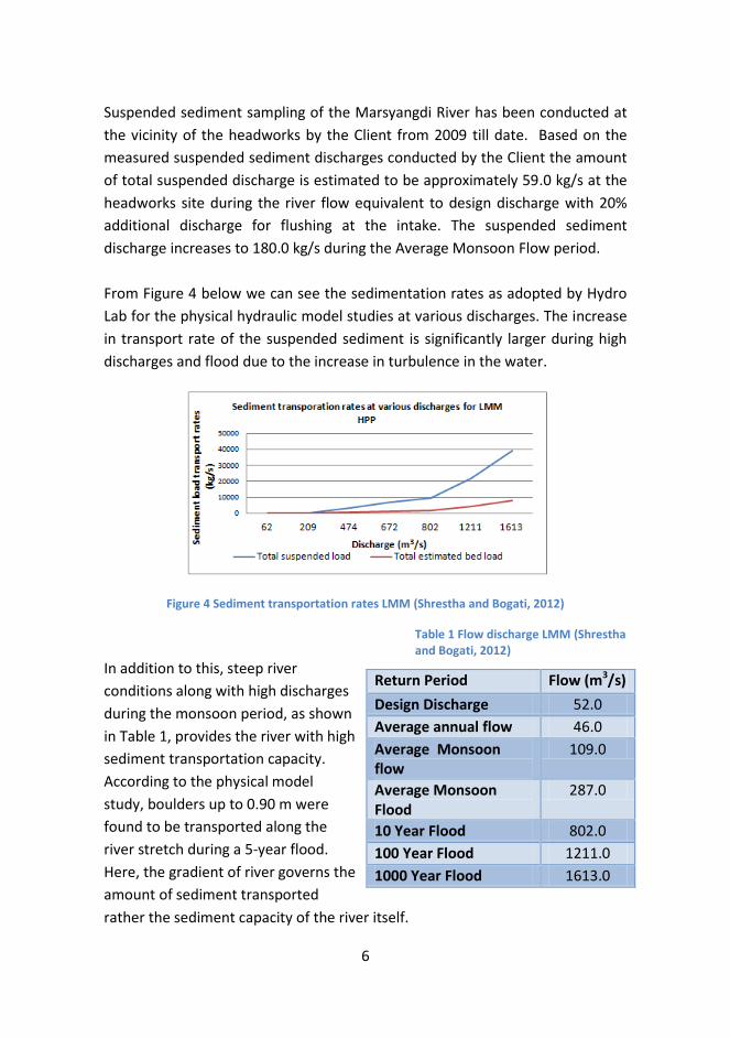
Suspended sediment sampling of the Marsyangdi River has been conducted at
the vicinity of the headworks by the Client from 2009 till date. Based on the
measured suspended sediment discharges conducted by the Client the amount
of total suspended discharge is estimated to be approximately 59.0 kg/s at the
headworks site during the river flow equivalent to design discharge with 20%
additional discharge for flushing at the intake. The suspended sediment
discharge increases to 180.0 kg/s during the Average Monsoon Flow period.
From Figure 4 below we can see the sedimentation rates as adopted by Hydro
Lab for the physical hydraulic model studies at various discharges. The increase
in transport rate of the suspended sediment is significantly larger during high
discharges and flood due to the increase in turbulence in the water.
Figure 4 Sediment transportation rates LMM (Shrestha and Bogati, 2012)
Table 1 Flow discharge LMM (Shrestha and Bogati, 2012)
In addition to this, steep river
conditions along with high discharges
during the monsoon period, as shown
in Table 1, provides the river with high
sediment transportation capacity.
According to the physical model
study, boulders up to 0.90 m were
found to be transported along the
river stretch during a 5-year flood.
Here, the gradient of river governs the
amount of sediment transported
rather the sediment capacity of the river itself.
Return Period Flow (m3/s)
Design Discharge 52.0
Average annual flow 46.0
Average Monsoon flow
109.0
Average Monsoon Flood
287.0
10 Year Flood 802.0
100 Year Flood 1211.0
1000 Year Flood 1613.0

7
The design discharge, 52.0 m3/s, is only available 33% of the time as shown
from the Flow duration curve in Figure 5 consequently problems related to
flushing arrangements may arise during operation and the designed power
generation is only possible three months during the monsoon period.
Figure 5 Flow Duration Curve LMM HPP (Shrestha and Bogati, 2012)
In addition to this, almost 80 % of the sediment particles are noted to be sand
particles with a diameter size of less than 2.00 mm. A particle size distribution
(PSD) curve for flows up to the average monsoon flow as prepared by Hydro
Lab is shown in Figure 6. Sediment handling at the intake and along the
settling basins therefore needs to be well taken care in order to minimize wear
and tear of the mechanical components in the system.
Figure 6 PSD for flow up to Average Monsoon Flow LMM HPP (Shrestha
and Bogati, 2012)

8
According to the test observations of the base case in the physical model,
which is the initial design of the project as provided by the client, the intake did
not appear to function optimally. Several problems were observed at the
intake. The design was incapable of maintaining bed control in front of the
intake; bed load sluices lacked sufficient suction capacity, which eventually led
to the clogging of intake. Similarly, turbulent flows near the intake led to
uneven flow distribution to and along the settling basins. Design with respect to
hydraulic performance of the headworks and its sustainability is reviewed and
discussed in further detail in Chapter 5.
9
3 Theoretical background
The following sections provide a theoretical background for the topics that are
dealt with in this thesis. Factors that affect the design of headworks in steep
sediment loaded rivers are discussed in chapter 3.1. Parameters related to
intake hydraulics and design of settling basin has been presented in further
detail under sections 3.1.2 and 3.1.3 respectively. Chapter 3.2 gives an
understanding of the model theory behind Physical hydraulic models.
Furthermore, the topic of numerical modeling is presented in chapter 3.3.
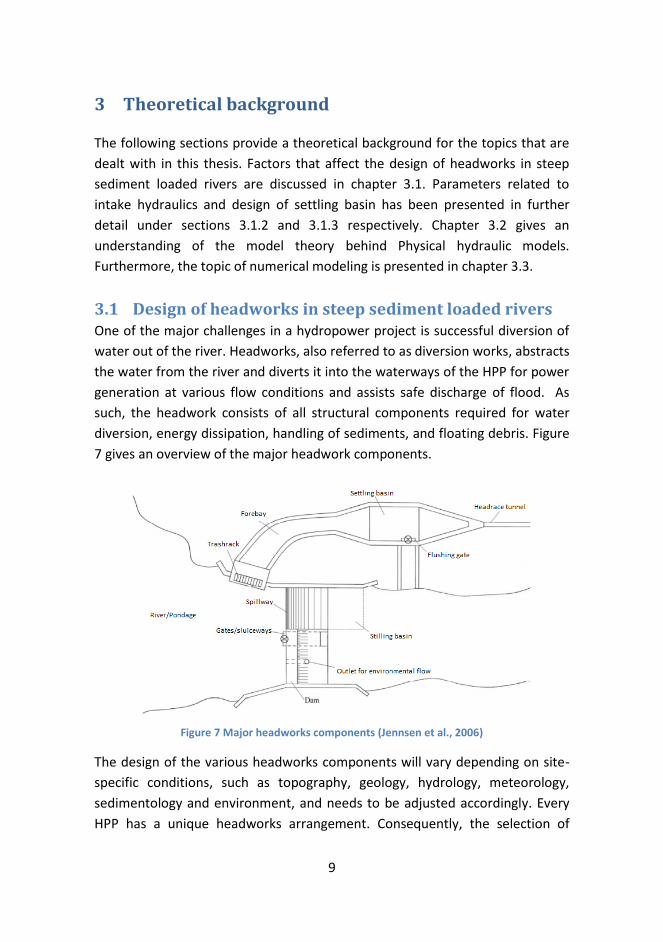
3.1 Design of headworks in steep sediment loaded rivers One of the major challenges in a hydropower project is successful diversion of
water out of the river. Headworks, also referred to as diversion works, abstracts
the water from the river and diverts it into the waterways of the HPP for power
generation at various flow conditions and assists safe discharge of flood. As
such, the headwork consists of all structural components required for water
diversion, energy dissipation, handling of sediments, and floating debris. Figure
7 gives an overview of the major headwork components.
Figure 7 Major headworks components (Jennsen et al., 2006)
The design of the various headworks components will vary depending on site-
specific conditions, such as topography, geology, hydrology, meteorology,
sedimentology and environment, and needs to be adjusted accordingly. Every
HPP has a unique headworks arrangement. Consequently, the selection of

10
headworks site should be based on the location’s technical, economic and
environmental suitability for the major components that form the headworks.
3.1.1 Performance standards
Poor performances of headworks causes reduced efficiency in the production
from the plant and leads to substantial economic losses. In order to address
concerns related to headworks design in a systematic way performance
standards developed by Lysne et al. (2003) have been discussed below.
Withdrawal of water
Headworks of a ROR plant needs to be capable of abstracting the amount of
water required for power generation and bypassing the surplus. The HPP have
to be designed such that the plants are able to extract design discharge from
the river even during dry season. Diversion weir (dam) along with the intake
diverts and controls the abstraction of water into the conveyance system.
A submergence of the intake is required so
that the water level in the river is high
enough for necessary abstraction of flow
even during dry seasons and for the
prevention of air entrainment in the
conveyance system. River training works
are used to provide favorable curvature of
flow near the intake. Guide walls are
usually constructed to constrain the flow
in front of the intake. The shape of the
guide wall and the alignment of the
intake should be designed to ensure a
uniform flow at the inlet of the intake. Turbulence is reduced due to the
smooth accelerating flow towards the intake. Figure 8 shows intake designs
that are undesirable and can create turbulent flow fields near the inlet.
Passage of floods, including hazard floods
The headworks structure needs to be designed to facilitate a safe passage of
the design flood without causing serious damages to the headworks. A flexible
headworks arrangement is required in the Nepalese rivers due to limited flow
records and uncertainties in the estimates. Flash floods due to natural hazards
Figure 8 Turbulent flow fields near the intake(Jennsen et al., 2006)
11
such as the Glacier lake outburst flood (GLOF) or overtopping should be
handled with some structural damages.
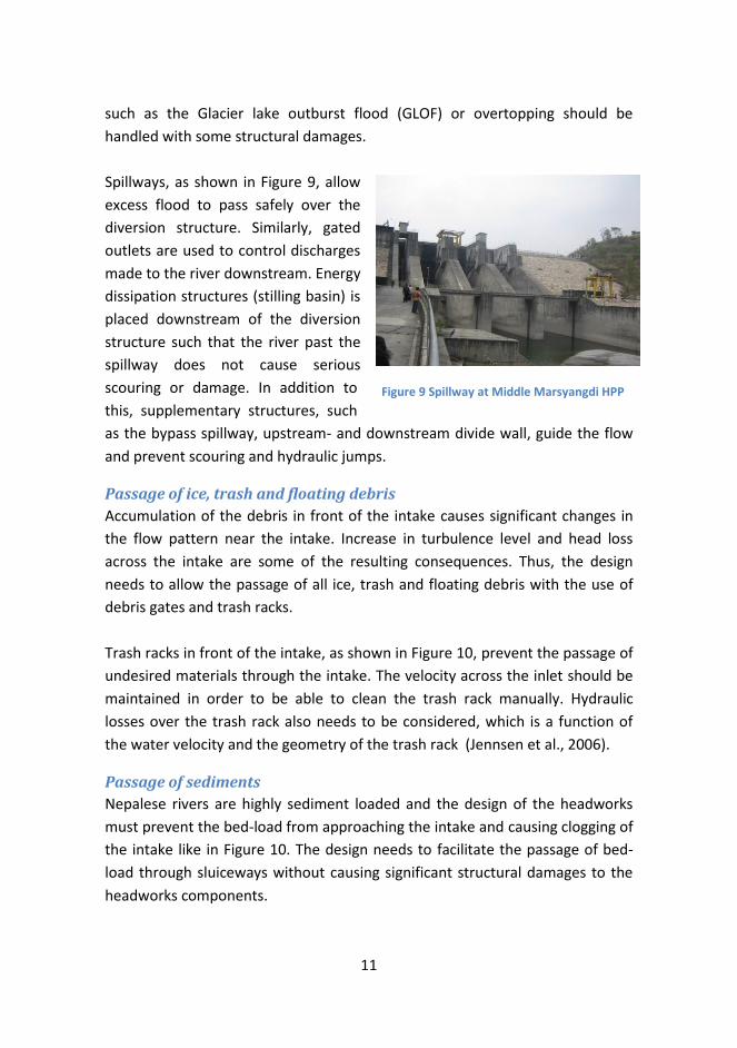
Spillways, as shown in Figure 9, allow
excess flood to pass safely over the
diversion structure. Similarly, gated
outlets are used to control discharges
made to the river downstream. Energy
dissipation structures (stilling basin) is
placed downstream of the diversion
structure such that the river past the
spillway does not cause serious
scouring or damage. In addition to
this, supplementary structures, such
as the bypass spillway, upstream- and downstream divide wall, guide the flow
and prevent scouring and hydraulic jumps.
Passage of ice, trash and floating debris
Accumulation of the debris in front of the intake causes significant changes in
the flow pattern near the intake. Increase in turbulence level and head loss
across the intake are some of the resulting consequences. Thus, the design
needs to allow the passage of all ice, trash and floating debris with the use of
debris gates and trash racks.
Trash racks in front of the intake, as shown in Figure 10, prevent the passage of
undesired materials through the intake. The velocity across the inlet should be
maintained in order to be able to clean the trash rack manually. Hydraulic
losses over the trash rack also needs to be considered, which is a function of
the water velocity and the geometry of the trash rack (Jennsen et al., 2006).
Passage of sediments
Nepalese rivers are highly sediment loaded and the design of the headworks
must prevent the bed-load from approaching the intake and causing clogging of
the intake like in Figure 10. The design needs to facilitate the passage of bed-
load through sluiceways without causing significant structural damages to the
headworks components.
Figure 9 Spillway at Middle Marsyangdi HPP

12
The run-of-river schemes in sediment-
loaded rivers need to be designed such
that most of the sediment is transported
along the river flow that is remaining after
abstraction of water into the waterways.
The transportation of sediment with the
river flow can be obtained by two ways
(Guttormsen, 2006) :
- Separation of the sediments
before the intake
- Flushing of sediments from the intake structure
The inlet of the intake needs to be placed above the intake bed such that the
bed load and sediments in the lower layer of the flow are separated from
upstream the intake at all flow conditions.
Bed control at the intake
In order to avoid the riverbed from
building up at the intake and causing
clogging and uneven flow distribution,
the intake either needs to be located
close to the spillway gates or should be
equipped with under-sluices, as shown in
Figure 11.
Exclusion of suspended sediments
and air
Suspended sediments need to be removed from the diverted water with the
use of settling basins to avoid sediment problems in the waterways and the
hydraulic machineries. The design of settling basin, which is a key concept for
sediment exclusion in plants has been discussed in detail in section 3.1.4. In
order to avoid air entrainment problems in the conveyance system air vents
need to be designed.
Flushing of settled sediments
Efficient flushing of the sediments from the settling basins needs to be ensured
such that its capacity remains unaltered. The removal of sediment from the
Figure 10 Intake cloggage at Khudi HPP(Shrestha et al., 2008)
Figure 11 Undersluice slots at Middle Marsyangdi HPP (Nielsen and Rettedal, 2012)
Trash racks
13
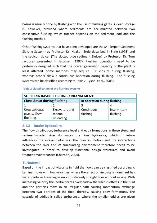
basins is usually done by flushing with the use of flushing gates. A dead storage
is, however, provided where sediments are accumulated between two
consecutive flushing, which further depends on the sediment load and the
flushing method.
Other flushing systems that have been developed are the S4 (Serpent Sediment
Sluicing System) by Professor Dr. Haakon Støle described in Støle (1993) and
the sedicon sluicer (The slotted pipe sediment Sluicer) by Professor Dr. Tom
Jacobsen presented in Jacobsen (1997). Flushing operations need to be
preferably designed such that the power generation capacity of the plant is
least affected. Some methods may require HPP closure during flushing,
whereas others allow a continuous operation during flushing. The flushing
systems can be classified according to Table 2 (Lysne et al., 2003):
Table 2 Classification of the flushing systems
SETTLING BASIN FLUSHING ARRANGEMENT
Close down during flushing In operation during flushing
1 Conventional gravity flow flushing
2 Excavators and manual unloading
3 Continuous flushing
4 Intermittent flushing
3.1.2 Intake hydraulics
The flow distribution, turbulence level and eddy formations in these steep and
sediment-loaded river dominates the river hydraulics, which in return
influences the intake hydraulics. The river in motion and the interactions
between the river and its surrounding environment therefore needs to be
investigated in order to develop functional design structures and avoid
frequent maintenances (Chanson, 2004).
Turbulence
Based on the impact of viscosity in fluid the flows can be classified accordingly.
Laminar flows with low velocities, where the effect of viscosity is dominant has
water particles traveling in smooth relatively straight lines without mixing. With
increasing velocity the inertial forces overshadow the viscous effects in the fluid
and the particles move in an irregular path causing momentum exchange
between two portions of the fluid, thereby, causing eddy formations. The
cascade of eddies is called turbulence, where the smaller eddies are given

14
energy by the largest eddies and the main flow provides energy to sustain the
lager eddies.
Which of these flows are dominant in a channel is dependent on the Reynolds
number, Re, which, is dependent on the velocity, u, characteristic length, L and
kinematic viscosity, ν.
ν (3.1)
In open channels such as a river, the flow is considered turbulent for a Reynolds
number above 12500. Figure 12 exhibits a typical point velocity measurement
in a turbulent flow regime with a steady mean value U and a fluctuating
component u’(t). A turbulent flow is here characterized by the mean value of its
velocities and a statistical property of their fluctuations (Versteeg and
Malalasekera, 2007).
Figure 12 Turbulent flow regimes (Oslen, 2011)
Turbulent kinetic energy (TKE)
Turbulent fluctuations always have a three dimensional spatial character given
as u’, v’,w’. The fluctuations are calculated as a standard deviation of the
measured velocity in the various flow directions. Turbulent kinetic energy per
unit mass at a particular point is then defined by the following equation:
(Versteeg and Malalasekera, 2007).
(3.2)
15
Turbulence Intensity
Similarly, the turbulence intensity, Ti, is defined using the average root mean
square velocity and is defined as follows:
(3.3)
Here, Uref is the reference mean velocity at a particular point.
Vorticity
Swirling motion in turbulent flows can also be characterized using the concept
of vorticity, which is defined by the curl of the fluid velocity along the fluids axis
of rotation.
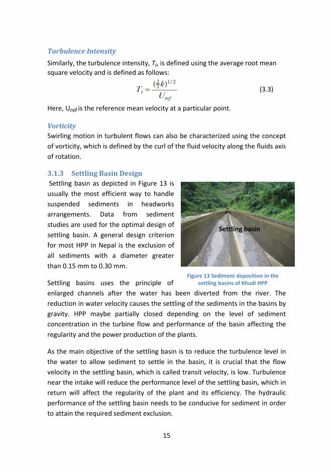
3.1.3 Settling Basin Design
Settling basin as depicted in Figure 13 is
usually the most efficient way to handle
suspended sediments in headworks
arrangements. Data from sediment
studies are used for the optimal design of
settling basin. A general design criterion
for most HPP in Nepal is the exclusion of
all sediments with a diameter greater
than 0.15 mm to 0.30 mm.
Settling basins uses the principle of
enlarged channels after the water has been diverted from the river. The
reduction in water velocity causes the settling of the sediments in the basins by
gravity. HPP maybe partially closed depending on the level of sediment
concentration in the turbine flow and performance of the basin affecting the
regularity and the power production of the plants.
As the main objective of the settling basin is to reduce the turbulence level in
the water to allow sediment to settle in the basin, it is crucial that the flow
velocity in the settling basin, which is called transit velocity, is low. Turbulence
near the intake will reduce the performance level of the settling basin, which in
return will affect the regularity of the plant and its efficiency. The hydraulic
performance of the settling basin needs to be conducive for sediment in order
to attain the required sediment exclusion.
Settling basin
Figure 13 Sediment deposition in the settling basins of Khudi HPP
16
There are several methods for computing the trapping efficiency of a settling
basin. A particle approach to trap efficiency as in the Camps or Shields method,
which are analytical methods, computes the probability of a single particle
being trapped in the settling basin as described in Lysne et al. (2003). Camps
diagram includes the effect of turbulence on the fall velocity of the particles,
where the fall velocity and thereby the trap efficiency increases with decrease
in turbulence level in the flow. Similarly, Vetter uses sediment concentration
and flow distribution as design criteria to evaluate the performance of the
settling basin. Vetter’s approach takes into consideration the difference in
average sediment concentration in the inlet flow to the settling basin and the
outlet flow from the basin.
Settling basins are recommended to have at least two chambers separated by
longitudinal divide walls, such that inspection and maintenance can be carried
out in one of the basins during the dry seasons without affecting the operation
of the power plant.
The hydraulic design of a settling basin arrangement needs to secure the
following (Lysne et al., 2003) :
An even flow distribution between parallel settling basins for various
flows
An even flow distribution internally inside each basin for various flows
Efficient removal of deposits during flushing of the basin
Size and shape of the basin are the major factors affecting its trap efficiency. A
larger basin helps in increasing the amount of sediments excluded and a good
shape of the basin produces even flow distribution in the basin increasing its
trap efficiency. The major components of a typical settling basin are shown in
Figure 14.
In order to achieve an even and optimum flow distribution along the basins
guide walls are commonly used at the inlet transition and slotted walls at the
outlet. The inlet transition and expansion is recommended to have a symmetric
layout with the length of the approach canal mounting to ten times the width
of the canal upstream of the expansion towards the settling basins. This helps
to avoid the effect of secondary currents, rotational flows, set by a bend in the

17
approach canal and to ensure that the velocities at the inlet are maintained in
the range, 1.1 to 1.3 m/s.
Figure 14 General layout of settling basin (Lysne et al., 2003)
A smooth and symmetric expansion including a small opening angle (φ/4), less
than 10 to 12 degrees, with the help of guide walls prevents the separation of
flow at the inlet transition. If the topography does not favor a symmetric
design, then pressurized canals can be used to accelerate the flow downstream
of a bend such that effects of secondary currents are nullified.
Flow tranquilizers, as shown in Figure
15, are filters where the flow is
distributed over a cross-section by
the use of head-loss. They are also
used to replace long and gentle inlet
transitions. However, both slotted
outlets and tranquilizers lead to an
extensive head-loss and will lead to
generation loss throughout the
lifetime of the plant and need careful
consideration and optimization before
usage (Lysne et al., 2003).
Figure 15 Flow tranquilizers at the inlet of
Settling basins in Lower Modi HEP
18
3.2 Model theory Physical hydraulic model (PHM) studies in general use reduced topographic and
structural scale. In order to gain comparable results between the prototype and
the model, scaling ratios of motion, forces and geometry needs to be
maintained. This is known as the law of similitude.
The geometric similitude, the similarity in form, is satisfied when the ratio of all
corresponding length, L, dimensions in the model and the prototype are the
same and can be given as follows:
Lr = Lm/Lp (3.4)
Here, index r denotes ratio whereas m and p respectively denote the model
and prototype.
The kinematic similitude is obtained when all the forces at geometrically
equivalent points have similarities in motion, constant velocity, v, and
acceleration, a.
Vr = Vm/Vp (3.5)
Dynamic similitude furthermore requires that the forces have same relative
directions and can be reduced by the same scale ratio and is a perquisite for
physical modeling.
Fr = Fm/Fp (3.6)
The dynamic laws of similitude are derived using Newton’s second law of
motion through a dimensional analysis ensuring that there is a constant model-
to-prototype ratio of all masses and forces acting on the system.
F = m * a (3.7)
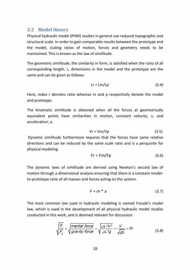
The most common law used in hydraulic modeling is named Froude’s model
law, which is used in the development of all physical hydraulic model studies
conducted in this work, and is deemed relevant for discussion.
(3.8)

19
The Froude law relates gravity and inertial forces, using the Froude number (Fr)
and neglects viscous forces and surface tension forces. River with free water
surface flow are gravity driven, turbulent (Reynolds number, Re>2000-3000)
and incompressible in nature due to which the almost all the models of rivers
and hydraulic structures are based on the Froude model law.
Following scale ratios, as shown in Table 3, are generated using the Froude
model law:
Table 3 Scale ratios for various parameters when using the Froude model law (Lysne, 1982)
Parameter Unit Relative scale
Length m Lr
Velocity m/s Lr1/2
Time S Lr1/2
Discharge m3/s Lr5/2
Area m2 Lr2
Volume m3 Lr3
However, some practical aspects and limitations of using a single model law
needs to be considered. When using only one model law, the model is
incapable of simulating all relevant forces in the model at the proper scale. For
example, it would be difficult to maintain the turbulence in the river during dry
season in some rivers such that the viscous forces and the surface tension
forces cannot be neglected. Similarly, air entrainment effects in the prototype
cannot be modeled using the Froude law. Laboratory effects due to the limited
space, model constructability, lack of instruments in the laboratory also needs
to be considered and the model structure needs to be optimized accordingly.
Moreover, Froude’s model law is valid for sediment particles with a grain size
up to 2.00 mm -3.00 mm based on Shield’s experiments. The law is still
applicable but with inaccuracies for smaller grain sizes up to 0.20 mm. For
particles smaller than 0.20 mm modeling becomes very complex as cohesive
forces between the particles dominate the grain stability. The sediment
particles are modeled with the selected scaling ratio based on sediment
measurements and estimates made for the prototype. As the rate of sediment
transport does not follow the Froude’s model law the amount of transported

20
sediment in the model is not comparable to the actual prototype value but is
used for qualitative information.
3.3 Numerical Modeling – CFD
With the evolution of increasingly powerful computers, numerical programs
have recently emerged aiming to act as an alternative to physical modeling.
Computational fluid dynamics has been attempted to predict complex water
flow patterns and model sediment transport instead of physical models. The
major advantages here are savings in cost and time. However, due to its
limitations such as instability in calculations and difficulties in obtaining
convergence, physical modeling is still preferred. A number of cases have
previously been studied to develop and enhance the use of CFDs. The studies
have focused on validating the numerical simulations with data from the
physical models to assure its usability and sufficient quality in the results.
3.3.1 Grids
In numerical modeling, the geometry is divided into a large number of
geometrical elements called grid cells, shown in Figure 16, and the equations
are solved in each of these cells. The cells in the entire geometry of the model
altogether form the grid and can be classified according to their shape,
orthogonality, structure, formations and movements.
Figure 16 Different type of grid structures (Hasaas, 2012)
3.3.2 Navier Stokes equations
The Navier stokes equation is a non-linear second order differential equation
based on the continuity equation and the momentum equation. The equation is
used to compute water velocity in numerical models and is derived based on
equilibrium forces on an infinitesimal volume of water in a laminar flow under
the assumption of mass conservation.

21
The equation is three dimensional and time-dependent and given in a tensor
notation such that the spatial variation in all directions is accounted for in the
computations. The equation consists of four terms in total. The left side of the
equation consists of two terms. The first term is the transient term and can be
neglected during steady flow conditions. The second term describes the
convection process. The first term on the right side is the pressure term and the
second term is the diffusive term and includes viscosity. The application of the
equation is restricted to incompressible flow and Newtonian fluids (Kettner,
2010).
(3.9)
3.3.3 Discretization methods
Discretization is the transformation of partial differential equations from one
cell to another, where the variable in one cell is a function of the variable in the
neighbor cells. The discretization of the physical equations along the grid can be
done in space and time.
Spatial discretization based on the Navier-Stokes/Euler equations can be
executed in several ways. The finite difference method employs the Taylor
series expansion for the discretization of the differential form of the flow
variables. Finite element method uses the integral formulation of Navier-
Stokes/Euler equations but can only be applied in unstructured grids. The finite
Volume method, also used in Star CCM+, utilizes the conservation law- the
integral formulation of Navier-Stokes/Euler equations through a finite control
volume (Balzek, 2005).
The finite volume method is further categorized into several schemes based on
the methods of estimating variables on the cell surfaces. A first order
discretization scheme uses only one cell upstream of the cell for discretization
whereas second order scheme uses two cells upstream of the cell for
discretization of equations.
Temporal discretization is applied for unsteady flows, which is categorized into
implicit and explicit methods depending on whether the spatial discretization is
based on values in time step j or j-1. An implicit solution uses values in the
former time step j, whereas an explicit solution uses time step j-1. Though the

22
use of explicit method is simpler, implicit method provides a more stable
solution.
3.3.4 Turbulence models
Modeling turbulence in flows is a significant problem in numerical modeling
and several methods are developed to model the effect of fluctuations in an
approximate manner. All the available models solve the Navier stokes
equations, however in different ways. As there is no exact way of modeling the
turbulence, the turbulence model needs to be selected to represent the flows
in reality.
Direct numerical simulation (DNS) model uses very fine grids such that
eddies are dissipated due to the kinematic viscosity in the grid.
Consequently, the computational requirements are extensive. The
model is also only applicable for simple flow problems with low
Reynold numbers in the order 104-106 (Balzek, 2005).
Large Eddy Simulation (LES) models uses very fine grids to solve larger
eddies based in computations, and a turbulence model for the smaller
structures. The spatial resolution of the grids can thus be lower than
DNS and the modeling complexity and simulation costs are relatively
reduced (Kettner, 2010).
Reynolds-Averaged Navier-Stokes (RANS) equations
(3.10)
RANS equations are time-averaged Navier-Stokes equations for steady state
situations with an additional term used to represent the transfer of momentum
due to fluctuations in the water flow. The challenge lies in modeling the
additional term known as the Reynolds-stress term.
Two different approaches are used in Star CCM+ to model the Reynold stress
term:
1. Eddy viscosity model uses the concept of turbulent viscosity to model
the Reynold stress term as the function of averaged flow variables. Boussinesq
approximation is often used for modeling.

23
The variable k is the turbulent kinetic energy, δij is the Kronecker delta, which is 1 if i=j and otherwise it is 0 and νT is the eddy viscosity.
(3.11) In Star CCM+ three different models that use the eddy viscosity to solve the Reynold stress term are available (Adapco, 2012).
K-epsilon (k-ε) model uses two partial differential equations, the turbulent
kinetic energy (TKE) and the dissipation (ε) of TKE to solve for eddy
viscosity. The eddy viscosity is modeled as an average for all three
directions. Thus, although the model is not very accurate it gives a good
compromise between robustness and accuracy.
K-omega model is an alternative to K- ε model and uses k and the specific
dissipation rate (ω), the rate per unit TKE instead of ε to solve for the eddy
viscosity. This model compared to the k- ε model has an improved
performance for boundary layers under difficult conditions due to pressure
gradients and is applied throughout the boundary layer.
Spallart-Allmaras model contrary to the above mention turbulence models
solves only one equation, the convection-diffusion equation, for the eddy
viscosity. The model is not suited for flows where complex recirculation
occurs in the flow field.
2. Reynold Stress Transport model solves the Reynolds stress term by
solving for all the components involved in the stress term. As a
result, the model accounts for effects of anisotropy due to strong
swirling motion, streamline curvature, rapid changes in strain rate
and secondary flows. However, the model requires significant
computational effort and time.
3.3.5 Stability and convergence
Numerical modeling is an iterative process and the initial variables need to be
adjusted in order to gain satisfactory results. Convergence criteria are based on

24
residual values. Residual values measure either the deviation between correct
values and the values in the current iteration or the difference between two
simultaneous iterations. Star CCM+ uses the latter. A low residual, usually less
than 0.001 indicates convergence (Oslen, 2011).
(3.12)
Instabilities occur when the residual values oscillate often and become very
high. Relaxation coefficients are used to weight cell variables that are used for
each iteration. The use of relaxation coefficients will give a slower convergence
speed; however, it will also help to avoid instabilities. Relaxation factors are
often lowered when the solution diverges because of instabilities (Oslen, 2011).
(3.13)
3.3.6 Courant Number
The Courant-Friedrichs-Lewy number is defined as follows (Courant et al.,
1956):
(3.14) Here, u denotes the velocity in x, y and z direction. Δx, Δy and Δz are the cell
sizes in respectively x,y and z directions and Δt is the time step between two
successive computations. The courant number defines how fast a particular
phase passes through a cell. If the courant number is larger than one then the
velocity of particle is understood to be so high that it passes through a cell in
less than the allocated time step. Thus, for a proper convergence of the
solution the convective courant number for a cell should be less than one.
25
4 Methodology
River hydraulics is one of the major factors leading to extensive sediment
transport into the waterways of a Hydropower plant (HPP) as discussed earlier.
The hydraulics of the river channel at the intake is special considered in this
thesis when studying the case of LMM headworks and the model studies of
Khudi HPP and Kabeli ‘A’ HPP conducted at Hydro Lab.
Turbulent flow field near the intake and the settling basin along with the effects
further downstream in the various structures is assessed with respect to
performance standard of the intake as a whole. The challenges in investigating
these complex flow fields and methods to diminish their effect are furthermore
established. Physical model study is used to understand the flow pattern at the
headworks.
The physical hydraulic model study implements the theoretical aspect of
headworks design during the assessment of the performance of LMM
headworks and comprises of the following parts. Based on the literature review
presented as the theoretical background to this study the concept of
headworks design is analyzed for the various case studies on headworks design
further in this work.
The case studies includes an evaluation of the given design and improvements
made on the headworks with focus on sediment handling arrangement and
hydraulics, both during normal conditions and during floods. Furthermore,
performance standards of the intake related to the study of flow patterns in the
intake area and the settling basins; bed control in front of the intake and
passage of floating debris has also been reviewed.
For the case study of LMM HPP velocity measurements has been conducted
using ADV and micro propeller current in the physical model to analyze the flow
patterns and hydraulics in the settling basins. The measured velocities are then
used to establish turbulence levels in the water by calculating the turbulent
kinetic energy. Results from the collected measurements are later used to
compare against the results from the numerical simulations in order to identify
the uncertainties and accuracies of a numerical model study. Uncertainties and
errors from the measurements are also evaluated and discussed.

26
Computational fluid dynamics (CFD) model is also used as an alternative
method to replicate the flow phenomenon using STAR CCM+. The reliability and
the accuracy of the software used is studied and the uncertainties and
limitations are identified.
The numerical model uses a 3D-Autocad model of the LMM HPP developed
from the drawings provided by Hydro Lab. Headworks geometry is then
imported from AutoCad into Star CCM+. Grids are generated for the model and
a reference model is developed with a standard setup of mesh and physics
conditions. Limitations of the numerical model including the boundary
conditions are determined and required data are simulated based on the setup
provided. Results are extracted and processed for comparison with the
measurements conducted in the physical hydraulic model. The work is
concluded with the analysis of performance of the proposed headworks
arrangement with focus on settling basin for the headworks of LMM HPP along
with the identification and evaluation of uncertainties and recommendations
for further work.
27
5 Physical hydraulic model study of the headworks of
LMM HPP
An efficient and proper planning and design of the various hydraulic parts of a
HPP requires a hydraulic model study as it is often difficult to compute all the
parameters involved and predict all the consequences. Hydraulic model of the
headworks of LMM HPP is therefore used to verify the analytical design by
carrying it out manually.
The Physical hydraulic model has been used to replicate flows and pressures of
a water flow in a small-scale version of the topography and structure that has
been studied. The structure that is to be studied is often referred to as the
prototype. Model construction of the river reach and the headworks prototype
have allowed the study of various parameters such as the flow pattern, slope
and velocities in a visual way. Immediate visualization of the designed solutions
have helped to increase the understanding of the physical processes. Extreme
conditions have been simulated on the model to ensure the safe design of
headworks structures. Although some simplifications are used to achieve the
similitude between the prototype and the model by the use of Froude model
law discussed in Chapter 3.2, a high degree of accuracy and reliability has be
attained by the use of empirical rules for the interpretation of the model tests.
5.1 Model study methodology The following general methodology have been applied when conducting the
physical model study (Shrestha and Bogati, 2012):
1. Field data on hydrology, river bed material and topography are
acquired.
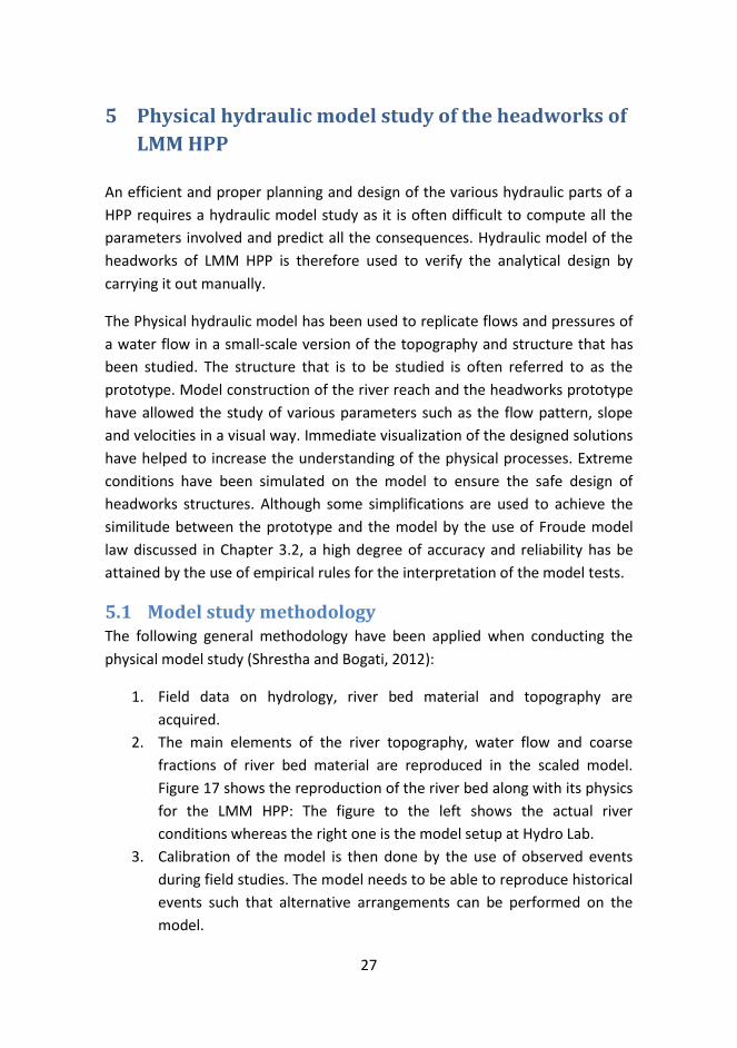
2. The main elements of the river topography, water flow and coarse
fractions of river bed material are reproduced in the scaled model.
Figure 17 shows the reproduction of the river bed along with its physics
for the LMM HPP: The figure to the left shows the actual river
conditions whereas the right one is the model setup at Hydro Lab.
3. Calibration of the model is then done by the use of observed events
during field studies. The model needs to be able to reproduce historical
events such that alternative arrangements can be performed on the
model.

28
4. Headwork structures are built in model scale and placed in the model.
Performance is simulated and bed movements and flow patterns are
observed and recorded under various flow conditions.
5. Problems are identified and alternative arrangements are suggested
and developed with the model study consultant/client.
6. The developed concept is verified through tests and the design is
optimized.
7. Tentative operational procedures can also be developed if operational
aspects of the final designs are simulated.
8. Critical phases of the construction process can also be studied by
rebuilding the model if needed.
Figure 17 Comparison of the model and prototype of the headworks site of LMM HPP (Shrestha and Bogati, 2012)
5.2 The initial design In order to evaluate the general hydraulic performance of the initial design as
provided by the Client a physical hydraulic model was developed at Hydro Lab
in a scale ratio of 1:40. The study of the initial design is based on the report
prepared by Shrestha and Bogati (2012) whereas the study of the modified
arrangement has been a combined effort of the author and the Hydro Lab team
working on the physical model of LMM HPP. As the model is yet to be finalized
for the final design, study conducted on the model during the author’s stay at
Hydro Lab has been focused and analyzed. The final arrangement mentioned
here is also the one that was finalized before the author’s departure from
Nepal.
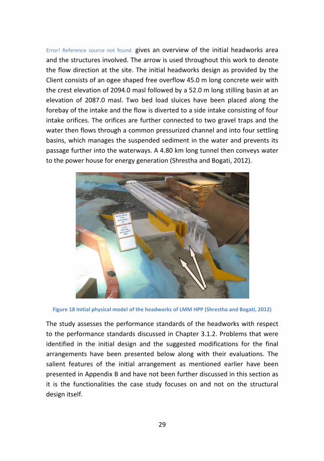
29
Error! Reference source not found. gives an overview of the initial headworks area
and the structures involved. The arrow is used throughout this work to denote
the flow direction at the site. The initial headworks design as provided by the
Client consists of an ogee shaped free overflow 45.0 m long concrete weir with
the crest elevation of 2094.0 masl followed by a 52.0 m long stilling basin at an
elevation of 2087.0 masl. Two bed load sluices have been placed along the
forebay of the intake and the flow is diverted to a side intake consisting of four
intake orifices. The orifices are further connected to two gravel traps and the
water then flows through a common pressurized channel and into four settling
basins, which manages the suspended sediment in the water and prevents its
passage further into the waterways. A 4.80 km long tunnel then conveys water
to the power house for energy generation (Shrestha and Bogati, 2012).
Figure 18 Initial physical model of the headworks of LMM HPP (Shrestha and Bogati, 2012)
The study assesses the performance standards of the headworks with respect
to the performance standards discussed in Chapter 3.1.2. Problems that were
identified in the initial design and the suggested modifications for the final
arrangements have been presented below along with their evaluations. The
salient features of the initial arrangement as mentioned earlier have been
presented in Appendix B and have not been further discussed in this section as
it is the functionalities the case study focuses on and not on the structural
design itself.

30
5.3 Analysis of the initial design against the Final
arrangement Several steady flow situations representing various return periods of flood
presented in Table 1 were tested to analyze the initial headworks design based
on its overall performance. In order to represent the bed load transport in the
river the model was continuously fed with sediments and gravels. Based on the
observations made during the tests significant problems were noted related to
the hydraulic performance and sedimentation in the vicinity of the headworks
site.
5.3.1 Intake Hydraulics
The initial design of the intake was capable of withdrawing the design discharge
(52.0m3/s). However, due to significant increase in velocities at higher flows
shooting flows were observed at the intake gates creating upwelling and
rotational flows in the gravel trap.
Slotted inlets, with a total of four
intake orifices for each intake, have
been provided in the final
arrangement to overcome local flow
circulations at the intake which leads
to the gravel trap and further to the
intake gates. In order to avoid
upwelling and any secondary current
effects at the intake the gates were
adjusted downstream of the gravel
traps. The gravel free discharge is
now conveyed through the intake
gate along the pressurized canals to the settling basins.
The main stream flow was diverted towards the intake at almost all flows that
were tested such that the intake was vulnerable to sediments and boulders.
Hence, a river training structure along with a guide wall has been placed along
the bed load sluice to create an outer bend effect at the intake orifices and
separate the bed load sluice from the weir. Similarly, sidewalls have been
placed along the right riverbank near the weir crest area to prevent erosion of
the side bank and gain a uniform flow towards the intake.
Figure 19 Final arrangement of the intake of the PHM of LMM HEP

31
Based on dye tests shown in Figure 19 some upwelling is still evident along the
approach canal, however the flow is observed to be calm and uniform along the
gravel trap. The turbulent flow along the stretch canal could be controlled by
regulating the opening of the bed load sluice gate.
Passage of floods
The initial design of the weir as shown in Figure 18 is assessed to be capable of
safely passing all flows including the design flood.
Although the energy dissipation in the stilling basin is found satisfactory,
erosive supercritical flow was observed downstream of the end sill when the
bed load sluices were in operation. The erosive flow had scouring effects on the
boulder riprap laid downstream. This scenario was mostly prevalent for the 2-
year return flood (discharge) and improved for higher flows. Due to a high flow
capacity of the bed load sluice shooting flows were observed from the bed load
sluiceways at higher flows (Figure 20). Thus, scouring effects were mostly
concentrated on the rightmost part of the stilling basin near the settling basin
wall threatening the basin’s stability.
Figure 20 Problems downstream on the inital arrangenement of the PHM of LMM HPP (Shrestha and Bogati, 2012)
The fan deposit of the China Khola at the downstream end of the headworks is
responsible for maintaining the tail water level. However, the deposits
especially on the right bank are observed to be susceptible to erosion at higher
floods and needs to be taken into consideration for further modifications.
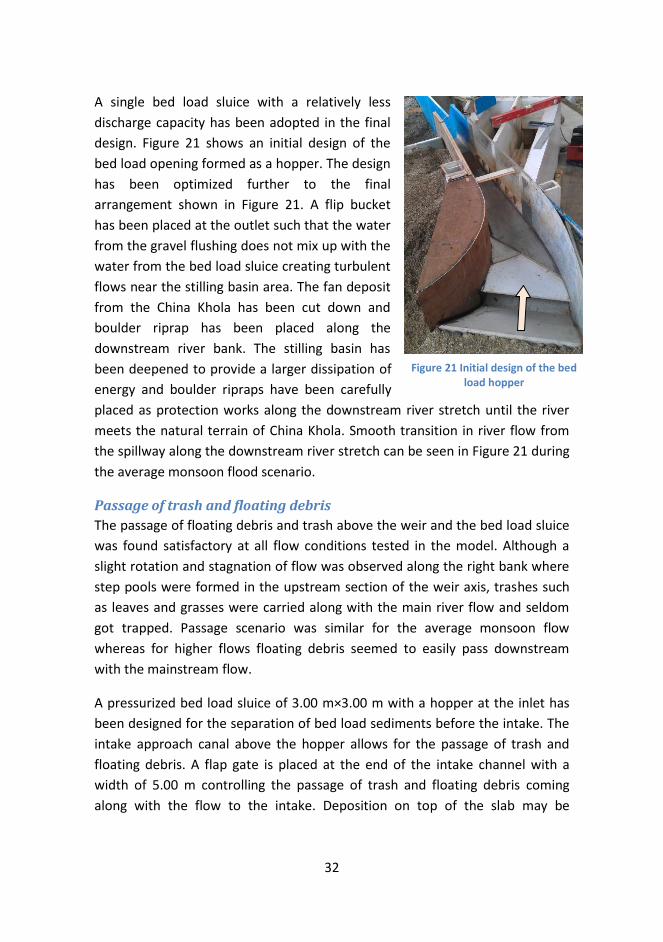
32
A single bed load sluice with a relatively less
discharge capacity has been adopted in the final
design. Figure 21 shows an initial design of the
bed load opening formed as a hopper. The design
has been optimized further to the final
arrangement shown in Figure 21. A flip bucket
has been placed at the outlet such that the water
from the gravel flushing does not mix up with the
water from the bed load sluice creating turbulent
flows near the stilling basin area. The fan deposit
from the China Khola has been cut down and
boulder riprap has been placed along the
downstream river bank. The stilling basin has
been deepened to provide a larger dissipation of
energy and boulder ripraps have been carefully
placed as protection works along the downstream river stretch until the river
meets the natural terrain of China Khola. Smooth transition in river flow from
the spillway along the downstream river stretch can be seen in Figure 21 during
the average monsoon flood scenario.
Passage of trash and floating debris
The passage of floating debris and trash above the weir and the bed load sluice
was found satisfactory at all flow conditions tested in the model. Although a
slight rotation and stagnation of flow was observed along the right bank where
step pools were formed in the upstream section of the weir axis, trashes such
as leaves and grasses were carried along with the main river flow and seldom
got trapped. Passage scenario was similar for the average monsoon flow
whereas for higher flows floating debris seemed to easily pass downstream
with the mainstream flow.
A pressurized bed load sluice of 3.00 m×3.00 m with a hopper at the inlet has
been designed for the separation of bed load sediments before the intake. The
intake approach canal above the hopper allows for the passage of trash and
floating debris. A flap gate is placed at the end of the intake channel with a
width of 5.00 m controlling the passage of trash and floating debris coming
along with the flow to the intake. Deposition on top of the slab may be
Figure 21 Initial design of the bed load hopper

33
removed by a slotted pipe system or with other methods and has not been
considered in the model study.
Passage of sediments
The design flow had the capacity of transporting cobbles up to 0.09 m in size.
Average monsoon flow had the capacity of transporting cobbles up to 0.16 m in
size. 2-years flood was observed to transport boulder between 0.60 m and 0.80
m whereas boulders up to 2.00m to 3.00 m in diameters were found
transported along the river stretch during the simulation of 10-years flood.
Consequently, due to the steepness of the river and its transporting capacity
mentioned above the upstream vertical face of the weir was exposed to
boulders approaching at higher floods. The impact from the boulders onto the
weir is expected to create severe damages.
Weir crest increment by 2.00 m to a level of 2096.0 masl helped to significantly
handle the bed load sediments along the river stretch. The increment of weir
crest decreases the gradient of the river and thereby the approach velocity of
the river and the transported boulders. Large boulders were now observed to
be transported mainly along the left bank and the fines were diverted towards
the intake with the increase in river flow (Figure 23).
Bed Control at the intake
During the design flow scenario the outer bend effect was significantly
noticeable near the intake area with deposition of fine sediment in the inner
bend such that the right bank where the intake was proposed seemed relatively
sediment free.
For flows with an additional 20% flushing
discharge to the design discharge and the
average monsoon flow sediment deposition
was observed in front of the intake, which
over time clogged the intake. Figure 22
shows building of the bed in front of the
intake and its partial clogging. Thus, it was
deduced that the bed load sluices had
Figure 22 Bed control at the initial arrangement of LMM HPP (Shrestha and
Bogati, 2012)
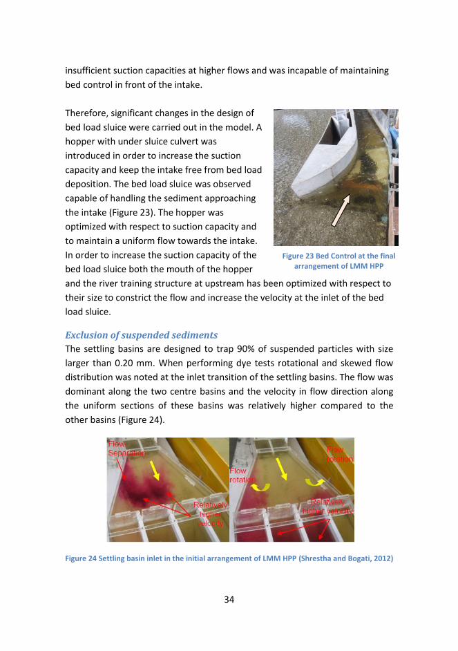
34
insufficient suction capacities at higher flows and was incapable of maintaining
bed control in front of the intake.
Therefore, significant changes in the design of
bed load sluice were carried out in the model. A
hopper with under sluice culvert was
introduced in order to increase the suction
capacity and keep the intake free from bed load
deposition. The bed load sluice was observed
capable of handling the sediment approaching
the intake (Figure 23). The hopper was
optimized with respect to suction capacity and
to maintain a uniform flow towards the intake.
In order to increase the suction capacity of the
bed load sluice both the mouth of the hopper
and the river training structure at upstream has been optimized with respect to
their size to constrict the flow and increase the velocity at the inlet of the bed
load sluice.
Exclusion of suspended sediments
The settling basins are designed to trap 90% of suspended particles with size
larger than 0.20 mm. When performing dye tests rotational and skewed flow
distribution was noted at the inlet transition of the settling basins. The flow was
dominant along the two centre basins and the velocity in flow direction along
the uniform sections of these basins was relatively higher compared to the
other basins (Figure 24).
Figure 24 Settling basin inlet in the initial arrangement of LMM HPP (Shrestha and Bogati, 2012)
Figure 23 Bed Control at the final arrangement of LMM HPP

35
Similarly, uneven flow was observed at the outlet transition of the basin where
the flow in the leftmost basin was almost negligible compared to the other
basins (Figure 25).
Based on the observed performance of the given
design, the approach culvert, transition, main
basins and the outlet of the settling basins was
redesigned to improve the hydraulic
performance. The settling basin (SB) approach
channel alignment and transition sections were
also modified. Alignment of single pressurized
approach channel was changed by introducing
two pressurized approach channels, which
provided a longer transition section to the
settling basins as shown in Figure26.
A divide wall has been provided along the approach channel until the start of
the uniform section of the settling basin to avoid flow separation and maintain
a uniform flow into the settling basin, designed with double hoppers. Based on
the dye test shown in Figure 27 for an Average Monsoon Flood scenario
relatively symmetrical and uniform flow conditions have been observed. The
hydraulic performance of the settling basins was consequently improved with
calm and uniform flow conditions from the start of the uniform section in the
basin.
Figure 25 Settling basin outlet in the initial arrangement of LMM HPP
Figure 26 Final arrangement of the SB of LMM HPP

36
Figure 27 Final arrangement of the approach canals in the PHM of LMM HPP
The settling basin outlet design has also been completely modified. A slot of
1.00 m opening has been placed at the outlet such that the effect from the
downstream flow onto the settling basin is nullified. Uniform flow conditions is
now seen at the outlet transitions from Figure 28.
Figure 28 Final arrangement on theSettling Basin outlet in the PHM of LMM HPP
Flushing of settled sediments
The S4 system is planned to be used for flushing of settled sediments from the
settling basin. Additional 10% of the design discharge abstracted from the river
through the intake is intended to be used for flushing of settled sediments at
the gravel trap and along the settling basin. Physical model study does not
include the study of the S4 system and flushing of the basins and has not been
assessed further in this study.

37
The final arrangement of the physical hydraulic model of the LMM HPP is
presented in Figure 29. The design as discussed in this Chapter has shown a
good conceptual performance and further optimization of the various
components are currently being carried out at Hydro Lab.
Figure 29 Final arrangement of the PHM of LMM HPP

38
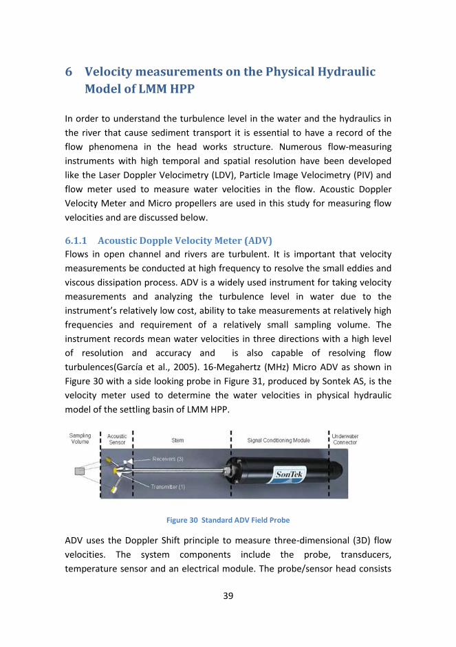
39
6 Velocity measurements on the Physical Hydraulic
Model of LMM HPP
In order to understand the turbulence level in the water and the hydraulics in
the river that cause sediment transport it is essential to have a record of the
flow phenomena in the head works structure. Numerous flow-measuring
instruments with high temporal and spatial resolution have been developed
like the Laser Doppler Velocimetry (LDV), Particle Image Velocimetry (PIV) and
flow meter used to measure water velocities in the flow. Acoustic Doppler
Velocity Meter and Micro propellers are used in this study for measuring flow
velocities and are discussed below.
6.1.1 Acoustic Dopple Velocity Meter (ADV)
Flows in open channel and rivers are turbulent. It is important that velocity
measurements be conducted at high frequency to resolve the small eddies and
viscous dissipation process. ADV is a widely used instrument for taking velocity
measurements and analyzing the turbulence level in water due to the
instrument’s relatively low cost, ability to take measurements at relatively high
frequencies and requirement of a relatively small sampling volume. The
instrument records mean water velocities in three directions with a high level
of resolution and accuracy and is also capable of resolving flow
turbulences(García et al., 2005). 16-Megahertz (MHz) Micro ADV as shown in
Figure 30 with a side looking probe in Figure 31, produced by Sontek AS, is the
velocity meter used to determine the water velocities in physical hydraulic
model of the settling basin of LMM HPP.
Figure 30 Standard ADV Field Probe
ADV uses the Doppler Shift principle to measure three-dimensional (3D) flow
velocities. The system components include the probe, transducers,
temperature sensor and an electrical module. The probe/sensor head consists
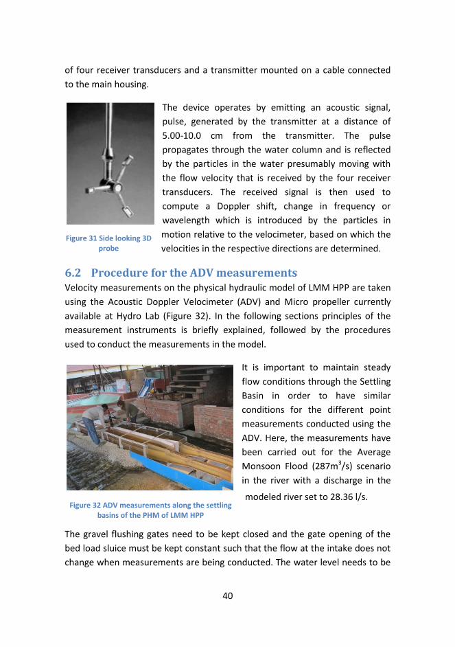
40
of four receiver transducers and a transmitter mounted on a cable connected
to the main housing.
The device operates by emitting an acoustic signal,
pulse, generated by the transmitter at a distance of
5.00-10.0 cm from the transmitter. The pulse
propagates through the water column and is reflected
by the particles in the water presumably moving with
the flow velocity that is received by the four receiver
transducers. The received signal is then used to
compute a Doppler shift, change in frequency or
wavelength which is introduced by the particles in
motion relative to the velocimeter, based on which the
velocities in the respective directions are determined.
6.2 Procedure for the ADV measurements Velocity measurements on the physical hydraulic model of LMM HPP are taken
using the Acoustic Doppler Velocimeter (ADV) and Micro propeller currently
available at Hydro Lab (Figure 32). In the following sections principles of the
measurement instruments is briefly explained, followed by the procedures
used to conduct the measurements in the model.
It is important to maintain steady
flow conditions through the Settling
Basin in order to have similar
conditions for the different point
measurements conducted using the
ADV. Here, the measurements have
been carried out for the Average
Monsoon Flood (287m3/s) scenario
in the river with a discharge in the
modeled river set to 28.36 l/s.
The gravel flushing gates need to be kept closed and the gate opening of the
bed load sluice must be kept constant such that the flow at the intake does not
change when measurements are being conducted. The water level needs to be
Figure 32 ADV measurements along the settling basins of the PHM of LMM HPP
Figure 31 Side looking 3D probe

41
stable. Here, the water level was stabilized to the prototype equivalent level of
2097.7 masl and the bed load sluice gate was kept at a constant opening
height. To prevent the impacts of wind onto the surface flow the settling basin
has been covered by thin wooden planks as it got rather windy during the
daytime while the measurements were taken.
Figure 33 Measured Cross-sections along the Settling Basins of LMM HPP
Six different cross sections (CS) shown in Figure 33 and Table 4 have been
decided for lab measurements along the settling basin. CS1 is the closest
section and has been placed right after the start of the uniform section in the
settling basin while CS6 is closest to the outlet. The sections have been divided
such that the measurements give a total overview of the flow scenario in the
settling basin.
Table 4 Measured Cross-sections along the Settling Basins of LMM HPP
Cross-sections Distance from the start of the uniform
section (Model values [mm])
Distance from the start of uniform
section (Prototype values [m])
CS1 350 14.0
CS2 1087 43.5
CS3 1824 73.0
CS4 2174 87.0
CS5 2962 118.5
CS6 3750 150.0
The ADV needs to be configured for proper collection of data. The velocity
range needs to be selected based on the expected range of data. A velocity
range of 3.00 cm/s has been chosen.
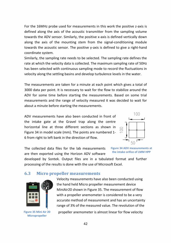
42
For the 16MHz probe used for measurements in this work the positive z-axis is
defined along the axis of the acoustic transmitter from the sampling volume
towards the ADV sensor. Similarly, the positive x-axis is defined vertically down
along the axis of the mounting stem from the signal-conditioning module
towards the acoustic sensor. The positive y-axis is defined to give a right-hand
coordinate system.
Similarly, the sampling rate needs to be selected. The sampling rate defines the
rate at which the velocity data is collected. The maximum sampling rate of 50Hz
has been selected with continuous sampling mode to record the fluctuations in
velocity along the settling basins and develop turbulence levels in the water.
The measurements are taken for a minute at each point which gives a total of
3000 data per point. It is necessary to wait for the flow to stabilize around the
ADV for some time before starting the measurements. Based on some trial
measurements and the range of velocity measured it was decided to wait for
about a minute before starting the measurements.
ADV measurements have also been conducted in front of
the intake gate at the Gravel trap along the centre
horizontal line at three different sections as shown in
Figure 34 in model scale (mm). The points are numbered 1-
6 from right to left bank in the direction of flow.
The collected data files for the lab measurements
are then exported using the Horizon ADV software
developed by Sontek. Output files are in a tabulated format and further
processing of the results is done with the use of Microsoft Excel.
6.3 Micro propeller measurements Velocity measurements have also been conducted using
the hand held Micro propeller measurement device
MiniAir20 shown in Figure 35. The measurement of flow
with a propeller anemometer is considered to be a very
accurate method of measurement and has an uncertainty
range of 3% of the measured value. The revolution of the
propeller anemometer is almost linear for flow velocity
Figure 34 ADV measurements at the intake orifice of LMM HPP
Figure 35 Mini Air 20 Micropropeller

43
and is furthermore independent from physical parameters such as pressure,
temperature, density and humidity.
In order to understand the flow conditions at the intake orifices velocity
measurements were conducted using Micro propeller. The velocity during a
period of 10s was averaged to determine the average water velocity passing
through the orifice. The measurements were conducted at three different
points along the top of each intake orifice shown as circular points in Figure 36.
The measurements here are given in millimeter (mm) based on the model
scale. The intake orifices have been numbered from 1-8 in the flow direction
when processing the results. In order to gain comparable results with the ADV
measurements made at the gravel trap propeller measurements have also been
conducted in front of the intake gate at similar cross-sections as shown in
Figure 34.
Figure 36 MicroPropeller measurements at the intake of the PHM of LMM HPP

44

45
7 Numerical model study of the headworks of LMM
HPP
The Numerical model study requires the usage of two different software
programs. AutoCAD has been used to replicate the 3D geometry of the physical
hydraulic model (PHM) of LMM HPP based on the 2D plan drawings obtained
from Hydro Lab shown in Appendix D. The numerical model has the same scale
ratio as the PHM of 1:40. The geometry has been developed as an STL (stereo
lithography) format such that it is supported by STAR-CCM+, in which the
simulation has been performed.
7.1 Star CCM+ The numerical simulations made in this report have been performed using the
Star CCM+ version 7.04.011 developed by CD Adapco. The spatial discretization
is done based on the Finite volume method and can handle structured and
unstructured grids. Surface repair tools in the solver allow for the processing
and simulation on the geometry extracted from AutoCAD files in order to
enhance the quality of geometry in the model. The program has an automatic
meshing technology and mesh models. Similarly, a range of physical models
with respect to time, solver, flow phases and turbulence models are provided
that can be combined depending on modeling needs.
Furthermore, plots and scenes of the results can be developed post simulation
in order to analyze and get a comprehensive visual understanding of the model
results. These results can be tabulated and exported if necessary. The program
uses a client-server architecture based on Java which handles the user
interface. The server, which computes the simulations, can run in serial or
parallel both with and without the client (Adapco, 2012).
7.2 The numerical model setup
7.2.1 Pre-processing
The imported stl-file from AutoCAD, as shown in Figure 37, provides the
program with the necessary geometry to start the numerical model study. As
the numerical model is drawn in the model scale ratio of the PHM the basic unit
used for drawing is millimeter (mm) scale. The co-ordinate system in the model
is defined such that the positive x-axis represents the direction of flow. The
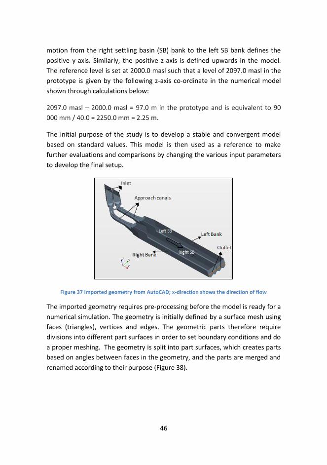
46
motion from the right settling basin (SB) bank to the left SB bank defines the
positive y-axis. Similarly, the positive z-axis is defined upwards in the model.
The reference level is set at 2000.0 masl such that a level of 2097.0 masl in the
prototype is given by the following z-axis co-ordinate in the numerical model
shown through calculations below:
2097.0 masl – 2000.0 masl = 97.0 m in the prototype and is equivalent to 90
000 mm / 40.0 = 2250.0 mm = 2.25 m.
The initial purpose of the study is to develop a stable and convergent model
based on standard values. This model is then used as a reference to make
further evaluations and comparisons by changing the various input parameters
to develop the final setup.
Figure 37 Imported geometry from AutoCAD; x-direction shows the direction of flow
The imported geometry requires pre-processing before the model is ready for a
numerical simulation. The geometry is initially defined by a surface mesh using
faces (triangles), vertices and edges. The geometric parts therefore require
divisions into different part surfaces in order to set boundary conditions and do
a proper meshing. The geometry is split into part surfaces, which creates parts
based on angles between faces in the geometry, and the parts are merged and
renamed according to their purpose (Figure 38).

47
Figure 38 Surface parts in the NHM
Furthermore, the surface needs to be examined for serious errors (Figure 39).
Surface diagnostics is used to repair the surface mesh to ensure that the
number of pierced faces, free edges, non-manifold edges and non-manifold
vertices are zero. Non-manifold edges are not shared by more than two
triangles. Poor quality faces were also observed due to the triangles used in
creating the shape of the surface since certain parts of the surface geometry
had very sharp angles. However, they were not considered to be problematic
for further simulations and have not been repaired.
Figure 39 Surface diagnostics of the NHM
The different geometric parts are then assigned into regions such that computations could be made in the various parts. A region is assigned for each part. Similarly, a boundary per part surface is selected for the creation of boundaries for each part surface. A feature curve per part curve has been

48
selected to define the sharp edges and the surface details that need to be maintained in the final volume mesh. The continuum of the model i.e. the mesh generation and the physics of the
model were then selected along with the boundary conditions in order to
create a functional model.
Mesh generation
A mesh continuum is a collection of the meshing models used to generate mesh
for the input geometry. Two different types of mesh models are available:
surface mesh and the volume mesh. The generation of the surface mesh
improves the triangulation of the surface in addition to the surface repair such
that a higher quality mesh is obtained. A high quality generation of a volume
mesh is therefore highly dependent on the quality of surface mesh. A surface
wrapper is used when the imported geometry is of extremely poor quality and
creates a closed surface. The quality of the model has been increased after the
surface repair and therefore a surface remesher is selected to re-triangulate
poor quality closed surfaces. Table 5 gives an overview of the selected mesh
models.
Table 5 Overview of the selected mesh models
Trimmer meshing model is composed predominantly of hexahedral cells with
trimmed cells next to the surface and are based on orthogonal mesh structure.
Trimmed cells are polyhedral cells that are usually recognized as hexahedral
cells with one or more corners and/or edges cut off. Tetrahedral model
comparatively is the fastest method for mesh generation and uses the least
amount of memory. Thin model is suited for thin geometries as the cell shapes
are decided accordingly. Polyhedral mesh type develops significantly fewer cells
than a tetrahedral model and is finer close to the geometries. Trimmer model
being a combination of polyhedral and hexahedral cells provides the basis for
Mesh type Selected meshing models
Alternative mesh models
Surface mesh
Surface remesher Surface wrapper
Volume mesh
Trimmer Polyhedral mesher Tetrahedral mesher Thin mesher
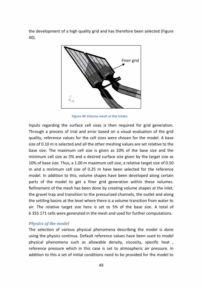
49
the development of a high quality grid and has therefore been selected (Figure
40).
Figure 40 Volume mesh at the intake
Inputs regarding the surface cell sizes is then required for grid generation.
Through a process of trial and error based on a visual evaluation of the grid
quality, reference values for the cell sizes were chosen for the model. A base
size of 0.10 m is selected and all the other meshing values are set relative to the
base size. The maximum cell size is given as 20% of the base size and the
minimum cell size as 5% and a desired surface size given by the target size as
10% of base size. Thus, a 1.00 m maximum cell size, a relative target size of 0.50
m and a minimum cell size of 0.25 m have been selected for the reference
model. In addition to this, volume shapes have been developed along certain
parts of the model to get a finer grid generation within these volumes.
Refinement of the mesh has been done by creating volume shapes at the inlet,
the gravel trap and transition to the pressurized channels, the outlet and along
the settling basins at the level where there is a volume transition from water to
air. The relative target size here is set to 5% of the base size. A total of
6 355 171 cells were generated in the mesh and used for further computations.
Physics of the model
The selection of various physical phenomena describing the model is done
using the physics continua. Default reference values have been used to model
physical phenomena such as allowable density, viscosity, specific heat ,
reference pressure which in this case is set to atmospheric air pressure. In
addition to this a set of initial conditions need to be provided for the model to
Finer grid
50
run. For unsteady-state simulations the converged solution is dependent on the
initial properties in the model and affects the path to convergence and the
computational effort required. Standard constant values enabled in the model
have been used as reference values for the initial conditions of pressure,
turbulence and velocity. The initial water level in the model is set using a field
function to gain the desired water level that is based on the lab measurements.
Field functions allow for the creation of a function which is used to describe the
flow conditions in the model. A field function called the initial water level was
therefore established:
($$Position[2]<=2.4425)?1:0
Here, Postion [2] is the z-direction of the model with upwards direction defined to be positive. According to the function, the initial water level is set at 2.4425m and the presence of water is defined beneath and at this level in the model volume. Table 6 gives an overview with a general description of the selected models with the alternatives available in STAR CCM+.
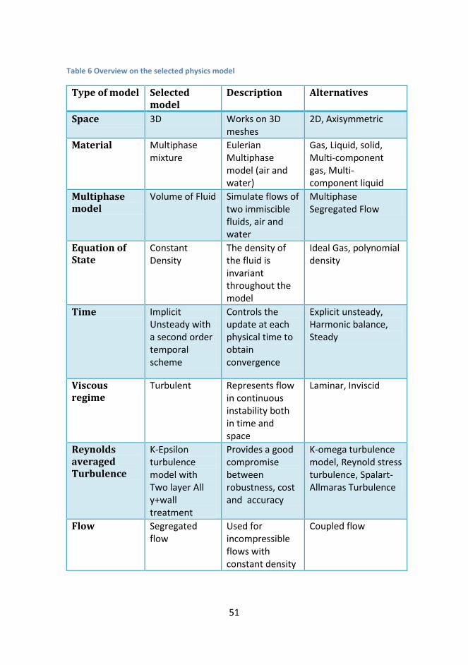
51
Table 6 Overview on the selected physics model
Type of model Selected model
Description Alternatives
Space 3D Works on 3D meshes
2D, Axisymmetric
Material Multiphase mixture
Eulerian Multiphase model (air and water)
Gas, Liquid, solid, Multi-component gas, Multi-component liquid
Multiphase model
Volume of Fluid Simulate flows of two immiscible fluids, air and water
Multiphase Segregated Flow
Equation of State
Constant Density
The density of the fluid is invariant throughout the model
Ideal Gas, polynomial density
Time Implicit Unsteady with a second order temporal scheme
Controls the update at each physical time to obtain convergence
Explicit unsteady, Harmonic balance, Steady
Viscous regime
Turbulent Represents flow in continuous instability both in time and space
Laminar, Inviscid
Reynolds averaged Turbulence
K-Epsilon turbulence model with Two layer All y+wall treatment
Provides a good compromise between robustness, cost and accuracy
K-omega turbulence model, Reynold stress turbulence, Spalart-Allmaras Turbulence
Flow Segregated flow
Used for incompressible flows with constant density
Coupled flow
52
Boundary conditions
The various surface parts when assigned to regions are developed as
boundaries. Boundaries are lines that surround and enclose these surface parts.
The various boundaries are assigned to boundary types based on the desired
physics for these boundaries. The boundary-types used in this model are mass-
flow inlet, pressure outlet, and walls. The mass flow inlet boundary is used for
incompressible flows to represent physical conditions such as flow direction-,
turbulence-, and velocity specification at the inlet when the mass flow rate is
known.
Wall boundary types are impermeable surfaces. Pressure outlet boundary is
used when the pressure is specified and is used in combination with mass-flow
inlet. The passing water then has no influence on the flow upstream the outlet
and the mass-flow at the inlet is equivalent to the mass flow sum at outlet
when the model is converged. For the model in question, a mass-flow inlet has
been assigned to inlet boundaries. The outlet and the top is set as a pressure
outlet while the rest of the boundaries is selected to be walls and have similar
physics as the bottom of the model.
Boundary conditions are then specified for each of the boundary types. Error!
Reference source not found. on the next page gives an overview of the
boundary conditions selected for the various boundary types along with
alternative methods that could have been used.
The values for the wall boundary types are similar where default values have
been used to define the blended wall function for walls with no slip conditions.
Default values based on the physics continua have also been used to describe
the physics of the outlet and the turbulence of the inlet. The turbulent intensity
is set as a lower limit of 0.01 and a turbulent viscosity ratio is set to 10.0 at both
the inlet and the outlet. Pressure at the outlet is set using a field function to
gain a correct pressure level above the slotted outlet. Field functions allow for
the creation of a function, which is used to describe the flow conditions in the
model. A field function called the pressure outlet was therefore established:
$Density*9.81*(2.4425-$$Position[2])
Here, Position [2] is the z-direction of the model with upwards direction
defined to be positive. According to the function, the pressure at the outlet is
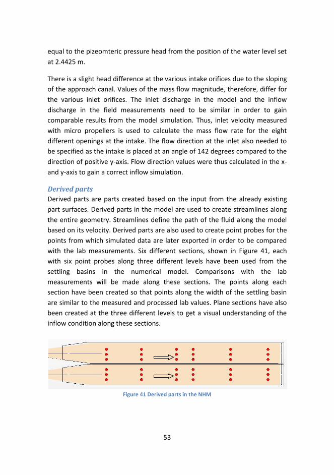
53
equal to the pizeomteric pressure head from the position of the water level set
at 2.4425 m.
There is a slight head difference at the various intake orifices due to the sloping
of the approach canal. Values of the mass flow magnitude, therefore, differ for
the various inlet orifices. The inlet discharge in the model and the inflow
discharge in the field measurements need to be similar in order to gain
comparable results from the model simulation. Thus, inlet velocity measured
with micro propellers is used to calculate the mass flow rate for the eight
different openings at the intake. The flow direction at the inlet also needed to
be specified as the intake is placed at an angle of 142 degrees compared to the
direction of positive y-axis. Flow direction values were thus calculated in the x-
and y-axis to gain a correct inflow simulation.
Derived parts
Derived parts are parts created based on the input from the already existing
part surfaces. Derived parts in the model are used to create streamlines along
the entire geometry. Streamlines define the path of the fluid along the model
based on its velocity. Derived parts are also used to create point probes for the
points from which simulated data are later exported in order to be compared
with the lab measurements. Six different sections, shown in Figure 41, each
with six point probes along three different levels have been used from the
settling basins in the numerical model. Comparisons with the lab
measurements will be made along these sections. The points along each
section have been created so that points along the width of the settling basin
are similar to the measured and processed lab values. Plane sections have also
been created at the three different levels to get a visual understanding of the
inflow condition along these sections.
Figure 41 Derived parts in the NHM

54
Table 7 Selected boundary conditions
Boundary Type
Physics conditions
Selected method
Alternatives
Intake Inlet Mass flow inlet
Flow direction specification
Components Boundary-Normal, Angles
Turbulence specification
Intensity + Viscosity ratio
K+epsilon, intensity + length scale
Velocity specification
Magnitude + Direction
Components
Settling Basin(SB) Outlet
Pressure outlet
Backflow Direction specification
Boundary-Normal
Extrapolated
Target mass flow option
Disabled Enabling the option
Turbulence specification
Intensity + Viscosity ratio
K + epsilon, intensity + length scale
Top Pressure outlet
Only mesh conditions as specified in the mesh continua
None None
Bottom Wall Shear stress specification
No-slip
Tangential velocity specification
None
Wall surface specification
Smooth Rough
Solvers and stopping criteria
Solvers are used to control the solution and are activated per iteration. The
solver is automatically selected in Star CCM based on the physics models that
have been selected. The difference between a solver and a model (mesh model
and the physics model) is defined by their limitation to the continuum. The
scope of the model is limited to the continuum selected whereas solvers can be
activated over the specified continua. Table 8 gives an overview of the solvers

55
used and the under-relaxation factor associated with each of the solvers. The
under-relaxation factors affect the convergence time and the number of inner
iterations required. A reduction in the under-relaxation factors leads to an
increase in the needed solution time for convergence and an increase in the
number of inner iterations.
Furthermore, stopping criteria are selected to limit the simulation run-time and
specify the conditions needed to stop iterating. The stopping criteria is
evaluated by the simulation model for each iteration and is stopped when the
criteria is satisfied. For an unsteady state model, which is used in this
simulation, the stopping criteria can be given by the maximum number of inner
iterations, maximum physical time or by the maximum number of steps. The
maximum number of iterations has been decided by evaluating the convergent
properties of the model and is set to 220000. The physical time step is set to
0.0015 s and the maximum number of inner iterations is set to 10 and involves
for each physical time-step the number of inner iterations required to converge
to a solution for a given cell.
Table 8 Under-relaxation factors used in the numerical model
Solver types Under–relaxation factor
Segregated flow velocity solver
0.8
Segregated flow Pressure solver
0.2
Segregated VOF solver 0.9
K-epsilon turbulence solver 0.8
K-epsilon turbulent viscosity solver
1.0
7.2.2 Post processing
Visualizing the solution
A visual analysis of the solution data in the model can be made in the graphics
window with the help of plots and scenes. Four different scenes including an
empty scene alternative are available in the program feature. The geometry
56
scene gives a view of the surface geometry. A mesh scene provides the same
visual as the geometry scene with enabled grid. Scalar scenes are used for
viewing scalar fields such as the velocity magnitude total pressure and vector
scenes for vector fields.
Plots based on reports of the simulation are also useful for analyzing solutions.
Mass inflow monitor plots have been used to decide the inlet velocity for the
model. The model velocity is adjusted such that the inflow stabilizes at
0.00689m3/s. The sum of mass flow is monitored to stabilize around zero such
that all incoming flow finds its way through the outlet. Similarly, residual plots
have been created to evaluate the stability and convergence of the model.
Result extraction
Velocity distributions in the various directions along with the turbulent kinetic
energy and vorticity have been extracted and tabulated for all the point probes
shown in Figure 41. The solution data from the simulation is exported into
Microsoft Excel and formatted and tabulated in a similar way as the velocity
measurements conducted in the physical hydraulic model of LMM such that the
two values become comparable. The points have been compared and analyzed
by using both graphs and plots in Chapter 8 and Chapter 9.

57
8 Results In this chapter results from the numerical simulation and velocity
measurements conducted in the physical hydraulic model of the headworks of
LMM are presented. Results and the uncertainties that follow are further
discussed and analyzed in Chapter 10.
8.1 Results from the numerical simulation In order to ensure that reliable results are achieved from the numerical
simulation, the convergence and mass flow balance from the simulation is
evaluated before presenting graphs and scenes showing the solutions from the
numerical simulation.
8.1.1 Reliability and convergence of the numerical simulation
Figure 42 below illustrates the development of residuals in the numerical
model with the iterations computed. The model is assumed converged when
the continuity residual is less than 0.001. The residual values fluctuate over an
average value of less than 0.001. From Figure 42 we see that the iterations
seem to have converged after 150 000 iterations over a value of 0.0001. To
ensure its consistency, however, the model has been enabled to run up to 220
000 iterations. The elapsed solution time for the unsteady simulations
performed is 33s. The solver iteration elapsed time is 0.217s per iterations,
which shows how long it took to execute each iteration giving a total solver
elapsed time of 15 hrs for the modeled simulation.
Figure 42 Residual plot of the numerical simulation
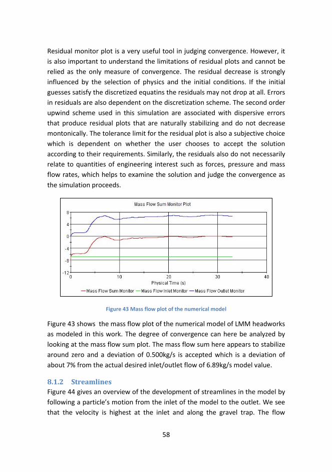
58
Residual monitor plot is a very useful tool in judging convergence. However, it
is also important to understand the limitations of residual plots and cannot be
relied as the only measure of convergence. The residual decrease is strongly
influenced by the selection of physics and the initial conditions. If the initial
guesses satisfy the discretized equatins the residuals may not drop at all. Errors
in residuals are also dependent on the discretization scheme. The second order
upwind scheme used in this simulation are associated with dispersive errors
that produce residual plots that are naturally stabilizing and do not decrease
montonically. The tolerance limit for the residual plot is also a subjective choice
which is dependent on whether the user chooses to accept the solution
according to their requirements. Similarly, the residuals also do not necessarily
relate to quantities of engineering interest such as forces, pressure and mass
flow rates, which helps to examine the solution and judge the convergence as
the simulation proceeds.
Figure 43 Mass flow plot of the numerical model
Figure 43 shows the mass flow plot of the numerical model of LMM headworks
as modeled in this work. The degree of convergence can here be analyzed by
looking at the mass flow sum plot. The mass flow sum here appears to stabilize
around zero and a deviation of 0.500kg/s is accepted which is a deviation of
about 7% from the actual desired inlet/outlet flow of 6.89kg/s model value.
8.1.2 Streamlines
Figure 44 gives an overview of the development of streamlines in the model by
following a particle’s motion from the inlet of the model to the outlet. We see
that the velocity is highest at the inlet and along the gravel trap. The flow
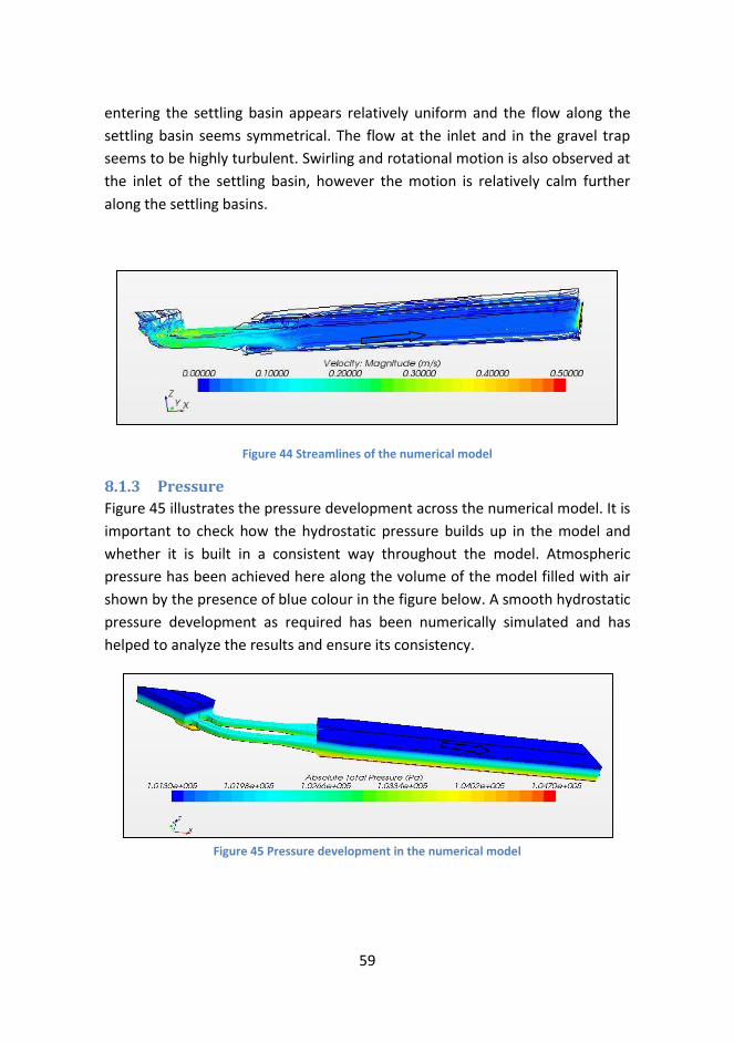
59
entering the settling basin appears relatively uniform and the flow along the
settling basin seems symmetrical. The flow at the inlet and in the gravel trap
seems to be highly turbulent. Swirling and rotational motion is also observed at
the inlet of the settling basin, however the motion is relatively calm further
along the settling basins.
Figure 44 Streamlines of the numerical model
8.1.3 Pressure
Figure 45 illustrates the pressure development across the numerical model. It is
important to check how the hydrostatic pressure builds up in the model and
whether it is built in a consistent way throughout the model. Atmospheric
pressure has been achieved here along the volume of the model filled with air
shown by the presence of blue colour in the figure below. A smooth hydrostatic
pressure development as required has been numerically simulated and has
helped to analyze the results and ensure its consistency.
Figure 45 Pressure development in the numerical model

60
8.1.4 Velocity distribution
Figure 46 shows the distribution of velocity along a plane section in the model.
As seen from the figure, the numerical model has not been capable of entirely
simulating the velocity distribution along the gravel trap. The velocities along
the gravel trap are very high in some cells and can be seen in further detail in
Figure 58. The mesh quality along the gravel trap probably influences the
results greatly and a finer grid may have solved the problem, which due to time
constraints has not been checked further. However, the flow fields in the gravel
trap are not considered to influence the velocities further in the settling basin
as a stable, uniform flow in the range expected is observed along the
pressurized section. The approach velocity seems relatively symmetrical and
uniform. A calm flow is observed along the settling basin with negligible
fluctuations in velocity. Desired flow is achieved along the settling basin, which
is discussed further in this chapter and has been further analyzed from the
turbulent kinetic energy values and tabulated velocity vectors in Chapter 9.
Figure 46 Velocity distributions along a plane section in the numerical model
8.1.5 Turbulent kinetic energy (TKE)
The turbulent kinetic energy as can be seen from Figure 47 is significantly
higher at the inlet and along the gravel trap with a maximum TKE value of 0.003
J/kg . TKE in the left approach canal in the flow direction seems to be slightly
higher though in the same range of magnitude suggesting skewed flow in the
pressurized section. However, the flow is rather symmetrical and uniform along
the inlet of the settling basins. Similarly, the turbulent kinetic energy is
observed to have decreased significantly from Cross-section 1 to Cross-section
2. The turbulent kinetic energy also seems to have stabilized from Cross-section
2 and equivalent along the length of the settling basins.
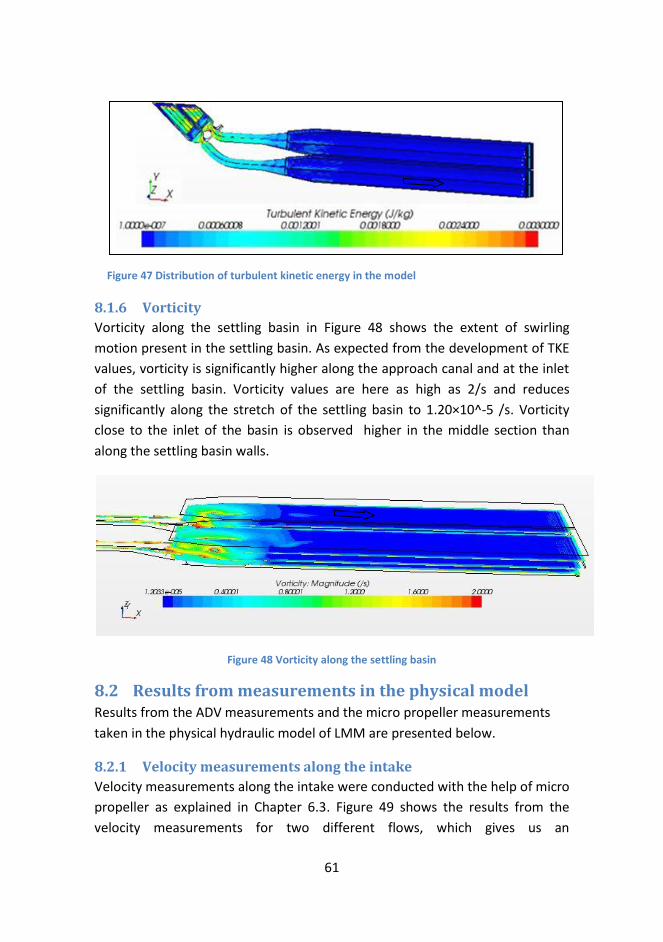
61
8.1.6 Vorticity
Vorticity along the settling basin in Figure 48 shows the extent of swirling
motion present in the settling basin. As expected from the development of TKE
values, vorticity is significantly higher along the approach canal and at the inlet
of the settling basin. Vorticity values are here as high as 2/s and reduces
significantly along the stretch of the settling basin to 1.20×10^-5 /s. Vorticity
close to the inlet of the basin is observed higher in the middle section than
along the settling basin walls.
Figure 48 Vorticity along the settling basin
8.2 Results from measurements in the physical model Results from the ADV measurements and the micro propeller measurements
taken in the physical hydraulic model of LMM are presented below.
8.2.1 Velocity measurements along the intake
Velocity measurements along the intake were conducted with the help of micro
propeller as explained in Chapter 6.3. Figure 49 shows the results from the
velocity measurements for two different flows, which gives us an
Figure 47 Distribution of turbulent kinetic energy in the model
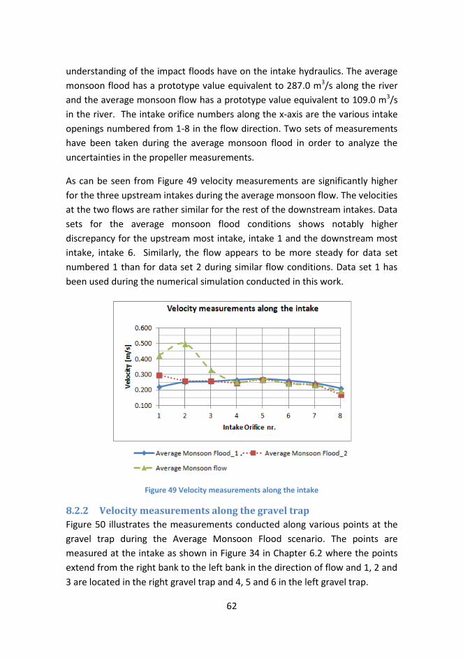
62
understanding of the impact floods have on the intake hydraulics. The average
monsoon flood has a prototype value equivalent to 287.0 m3/s along the river
and the average monsoon flow has a prototype value equivalent to 109.0 m3/s
in the river. The intake orifice numbers along the x-axis are the various intake
openings numbered from 1-8 in the flow direction. Two sets of measurements
have been taken during the average monsoon flood in order to analyze the
uncertainties in the propeller measurements.
As can be seen from Figure 49 velocity measurements are significantly higher
for the three upstream intakes during the average monsoon flow. The velocities
at the two flows are rather similar for the rest of the downstream intakes. Data
sets for the average monsoon flood conditions shows notably higher
discrepancy for the upstream most intake, intake 1 and the downstream most
intake, intake 6. Similarly, the flow appears to be more steady for data set
numbered 1 than for data set 2 during similar flow conditions. Data set 1 has
been used during the numerical simulation conducted in this work.
Figure 49 Velocity measurements along the intake
8.2.2 Velocity measurements along the gravel trap
Figure 50 illustrates the measurements conducted along various points at the
gravel trap during the Average Monsoon Flood scenario. The points are
measured at the intake as shown in Figure 34 in Chapter 6.2 where the points
extend from the right bank to the left bank in the direction of flow and 1, 2 and
3 are located in the right gravel trap and 4, 5 and 6 in the left gravel trap.

63
According to figure 50 the trends in velocity variations is mostly similar for the
propeller measurements and the ADV measurements along the gravel trap.
However, propeller measurements seem to overestimate the velocity
compared to the ADV measurements. Similarly, the velocities are higher in the
left gravel trap compared to the right gravel trap with a decreasing trend from
right to left bank along the flow direction. The velocity is highest at the right
end of the left gravel trap and at the centre of the right gravel trap. The
discrepancies between the two data sets are higher for the left gravel trap
compared to the right gravel trap.
Figure 50 Velocity measurements along the gravel trap
8.2.3 Comparison of measurements and simulations
In this sub-chapter the numerically simulated results from the numerical
hydraulic model of the headworks of LMM is compared to similar ADV
measurements taken at the physical hydraulic model at Hydro Lab.
Velocity measurements and simulations along the settling basin
Figure 51, Figure 52, and Figure 53 below show the plots of simulated and
measured velocities at various cross-sections along the settling basin.

64
Figure 51 Comparison of velocity field close to the bottom of the settling basin
Figure 52 Comparison of velocity field along the middle plane section of the settling basin
Figure 53 Comparison of velocity field close to the surface of the settling basin
ADV measurements along the plane section close to the bottom (z=2.21m)
show skewed flows along the first five cross-sections up to a length of 7.00 m
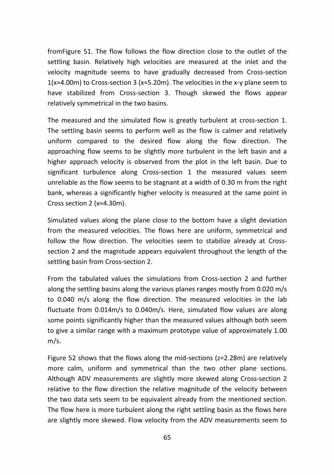
65
fromFigure 51. The flow follows the flow direction close to the outlet of the
settling basin. Relatively high velocities are measured at the inlet and the
velocity magnitude seems to have gradually decreased from Cross-section
1(x≈4.00m) to Cross-section 3 (x≈5.20m). The velocities in the x-y plane seem to
have stabilized from Cross-section 3. Though skewed the flows appear
relatively symmetrical in the two basins.
The measured and the simulated flow is greatly turbulent at cross-section 1.
The settling basin seems to perform well as the flow is calmer and relatively
uniform compared to the desired flow along the flow direction. The
approaching flow seems to be slightly more turbulent in the left basin and a
higher approach velocity is observed from the plot in the left basin. Due to
significant turbulence along Cross-section 1 the measured values seem
unreliable as the flow seems to be stagnant at a width of 0.30 m from the right
bank, whereas a significantly higher velocity is measured at the same point in
Cross section 2 (x≈4.30m).
Simulated values along the plane close to the bottom have a slight deviation
from the measured velocities. The flows here are uniform, symmetrical and
follow the flow direction. The velocities seem to stabilize already at Cross-
section 2 and the magnitude appears equivalent throughout the length of the
settling basin from Cross-section 2.
From the tabulated values the simulations from Cross-section 2 and further
along the settling basins along the various planes ranges mostly from 0.020 m/s
to 0.040 m/s along the flow direction. The measured velocities in the lab
fluctuate from 0.014m/s to 0.040m/s. Here, simulated flow values are along
some points significantly higher than the measured values although both seem
to give a similar range with a maximum prototype value of approximately 1.00
m/s.
Figure 52 shows that the flows along the mid-sections (z=2.28m) are relatively
more calm, uniform and symmetrical than the two other plane sections.
Although ADV measurements are slightly more skewed along Cross-section 2
relative to the flow direction the relative magnitude of the velocity between
the two data sets seem to be equivalent already from the mentioned section.
The flow here is more turbulent along the right settling basin as the flows here
are slightly more skewed. Flow velocity from the ADV measurements seem to
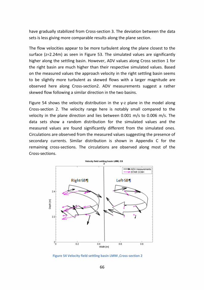
66
have gradually stabilized from Cross-section 3. The deviation between the data
sets is less giving more comparable results along the plane section.
The flow velocities appear to be more turbulent along the plane closest to the
surface (z=2.24m) as seen in Figure 53. The simulated values are significantly
higher along the settling basin. However, ADV values along Cross section 1 for
the right basin are much higher than their respective simulated values. Based
on the measured values the approach velocity in the right settling basin seems
to be slightly more turbulent as skewed flows with a larger magnitude are
observed here along Cross-section2. ADV measurements suggest a rather
skewed flow following a similar direction in the two basins.
Figure 54 shows the velocity distribution in the y-z plane in the model along
Cross-section 2. The velocity range here is notably small compared to the
velocity in the plane direction and lies between 0.001 m/s to 0.006 m/s. The
data sets show a random distribution for the simulated values and the
measured values are found significantly different from the simulated ones.
Circulations are observed from the measured values suggesting the presence of
secondary currents. Similar distribution is shown in Appendix C for the
remaining cross-sections. The circulations are observed along most of the
Cross-sections.
Figure 54 Velocity field settling basin LMM ,Cross-section 2

67
TKE along the settling basin
Figure 55 shows the development of turbulence along the settling basin based
on the numerical simulation. ADV measurements are shown for comparison
through circular nodes along the cross-sections in the same figure. Based on
this figure the initial turbulence level at the inlet level shown in cross-section 1
is equivalent to the simulated TKE values. A slight deviation can be noticed at
some points compared to the simulated values presented as the background of
these nodes. The simulated TKE values decreases rapidly from cross-section 1
to 2 and stabilizes thereafter. More accurate results of the TKE values are
shown through Figure 56.
Figure 55 Comparison of TKE development along the settling basin
Figure 56 shows a graphical presentation of the development of TKE along the
settling basin. A gradual decrease in the TKE values is observed for the ADV
measurements whereas a rapid decrease is observed from Cross-section 1 to 2
for the simulated values. There is a decrease in 3 orders of magnitude from
Cross-section 1 to 2 for the simulated values and the values appear constant at
1.00×10^-7. The discrepancy between the simulated values gets smaller along
the settling basins as the measured values decreases gradually. The measured
values decreases by one order of magnitude from Cross-section 1 to Cross-
section 6 from 3.0×10^-4 to 1.00×10^-5. The turbulence in the left and the right
settling basin appears symmetrical and uniform.
Right SB Left SB

68
Figure 56 TKE along the settling basin
Figure 57 illustrates the TKE distribution along Cross-section 4. The measured
TKE values here are one order of magnitude larger than the simulated values.
The trend is opposite for the two data sets. The measured values shows a slight
increase going from upwards in the positive z-direction from the bottom of the
settling basin, whereas the simulated values show a slight decrease in TKE
values along similar sections.
Figure 57 TKE at Cross-section 4

69
Velocity along the gravel trap
As high velocities were observed from, the numerical simulations at the inlet
for the pressurized section along the gravel trap comparisons of similar sections
have been made in Figure 58 . The circular nodes are values from ADV-
measurements whereas the background shows the numerically simulated
cross-section of the opening at gravel trap in the flow direction.
We observe that velocities at the centre point are quite similar, however
simulated velocities are significantly higher compared to the measured ones at
the inlet walls in Figure 58.
Turbulent Kinetic Energy (TKE) along the gravel trap
Based on Figure 59 the measured values show a significantly high level of
turbulence along the gravel trap with a maximum range of 0.003 J/kg.
Turbulence is also observed higher along the left gravel trap. TKE values here
Figure 59 TKE based on ADV measurements along the gravel trap
Figure 58 Velocity along the gravel trap
Right Gravel trap Left Gravel trap

70
are in the left gravel trap significantly larger than the ones simulated for Cross-
section 1 shown in Figure 59Figure 47. The TKE values for the measured data
are highest at the centre of each gravel trap and turbulence level along the left
settling basin is observed to be notably higher than the right gravel trap, which
is similar to the trend seen from the simulation results.
8.3 Vorticity in the numerical simulation
Based on Figure 60 the vorticity decreases gradually until Cross-section 3
(x≈5.20m) and then starts to increase at a smaller rate until Cross-section 6
(x≈7.00m) suggesting higher level of circulation close to the outlet and near the
inlet.
Figure 61 gives an overview of the development of vorticity at various depths
along the two settling basins at Cross-section 1 , 4 and 6. Circulation formation
is larger along the right basin (R) for Cross-section 1. The vorticity along the
right basin is less at Cross-section 4 compared to the left basin (L). Vorticity
development is relatively equivalent along Cross-section 6 as can be seen from
the above figure. Vorticity development along Cross-section 6 and Cross-
section 4 show a similar trend along the depth of the settling basin whereas
vorticity decreases with depth along Cross-section 1.
Figure 60 Simulation of vorticity along the settling basin

71
Figure 61 Simulated vorticity at various depths

72
73
9 Discussion This chapter briefly evaluates the study conducted at the physical hydraulic
model in Chapter 8 and analyzes the results presented in Chapter 9.
Furthermore, uncertainties in the results and measurements are also discussed
under each sub-chapter.
9.1 Physical Hydraulic Model studies of Headworks Based on experiences gained from the case studies conducted and the Physical
Hydraulic Model study of the LMM HPP the design of headworks is often a
compromise between the various performance standards mentioned in
Chapter 3.1.1 and the economic viability of the project. In river conditions with
steep, sediment-loaded rivers, it is extremely important to focus on the design
of settling basins while designing the overall headworks.
Existing power plants such as Khudi HPP discussed in Appendix A have been
subjected to clogging at the intake due to poor sediment management. The
ability of headworks to separate bed load before the intake or upstream of the
settling basins ensures that the abstracted water to the settling basins is free of
bed load. Separation of sediments and thereby a controlled bed at the intake is
obtained by the use of bed load sluices as in the case of Khudi HPP and LMM
HPP or undersluices as used in Kabeli ‘A’ HPP .
Flushing arrangements and operations of the flushing gates such as the bed
load sluice gate and the gravel trap flushing gate also need to be carefully
considered as these will have an impact on the hydraulics at and along the
intake. Lack of proper flushing head leads to reduced flushing efficiency and
thereby an increase in bed level in front of the intake causing larger amount of
sediment to be transported along the intake. A decrease in the efficiency of the
settling basin is then followed by passage of sediments through the conveyance
system causing erosion along the conveyance system and of the mechanical
components.
Passage of flood is also one of the major design considerations, however, this
rarely seems to be a problem in the reviewed projects. However, the design of
stilling basin needs to be considered for the proper dissipation of energy
especially during higher floods, as studied and observed for the PHM of Kabeli

74
‘A’ and LMM HPP. Furthermore, downstream areas that are susceptible to
erosion need to be protected with the use of riprap.
Intake hydraulics as seen for all three cases greatly affects the transport of
sediments near and along the intake. Use of river training structures to guide
the flow by securing the impact of an outer curvature along the intake orifices
both helps in diverting the sediments away from the intake and ensuring a
reasonably uniform flow towards the intake as discussed in Chapter 3.1.1.
Securing good hydraulics at the intake along with a proper floating debris
passage also aids in handling of trash and floating debris. Similarly, the use of
slots and divide walls to reduce the size of eddies formed in and along the
intake structures helps to secure the desired hydraulics at the intake structures.
Weir crest increment is also in some cases an effective way to reduce the
velocities in front of the intake such that sediment transport, especially of large
boulders that can create damages to the intake structure and disrupt the intake
hydraulics is significantly reduced.
A highly sediment loaded river in most cases requires both a bed load sluice
followed by a gravel trap and settling basins for proper sediment exclusion as
designed for the LMM HPP and Khudi HPP. As seen from these case studies the
PHM study is often used to improve the design of the settling basin structures
to ensure flow condtions as discussed in Chapter 3.1.3. The size and shape of
the settling basins needs to be designed in such a way that even flow
distribution for trapping of suspended sediments within the settling basins
along with efficient removal of deposits is secured. Symmetric layout of the
settling basins along with smooth transitions and use of divide walls along the
approach canal and inlet transition as theoretically explained in Chapter 3.1.3
was observed to be an effective way of securing symmetrical uniform flow
along the settling basins. Use of intermittent flushing is often a good
compromise between ensuring regularity in power generation capacity of the
plant and securing proper management of sediment. Slotted pipes and the S4
system have been recommended for the flushing arrangements of LMM HPP.
River hydraulics and sediment study is a complex process and specially in a
country such as Nepal where both the available data quantity and their quality
is questionable, analytical calculations are often not enough to secure a
functional headworks design. Thus, it is often difficult to foresee and

75
understand the functional aspect of the intake without a physical hydraulic
model study. Despite the scale effects discussed in Chapter 3.2 physical
hydraulic model study helps in studying both intake hydraulics and sediment
transport tendencies along the intake. Problems can then be identified and
improvements suggested through tests on the model to ensure a functional
design of headworks.
9.2 Measurements on the Physical Hydraulic Model Based on the comparisons made for the two data sets measured at the intake
for the Average Monsoon Flood condition it can be concluded that micro
propeller measurements are of good quality. The accuracy of the data is
difficult to validate as only micro propeller was used to measure along the
intake. According to the specifications from the company that designed the
propeller the instrument has an uncertainty range of 3% of the measured value.
The variations at inlet 1 can be caused by standing waves and turbulence
observed near the intake above the bed load hopper when the measurement
was taken. Similarly, the variations at inlet 8 could be due to a difference in
regulation of the flap gate used for the passage of trash and debris while the
measurements were taken. The presence of a gate disrupts the flow and back
flows might create variations in the velocity fields near inlet 8. Discrepancies in
the two flow conditions presented are the result of varying operations of bed
load sluice gate and the trash passage gate.
Based on the velocity measurements in the gravel trap, Micro propeller seems
to overestimate the velocity compared to the ADV measurements along the
similar stretch. The propeller averages the velocity measured during an interval
of 10.0 s such that the velocity ranges become higher during this interval. The
ADV measurements are point measurements at an interval of 1.00 s and
records 50 data per measurements including the rapid fluctuations in velocity.
ADV measurements are thus more accurate point measurements whereas the
Micro propeller can be used to estimate the upper ranges of velocity fields in
the flow. The velocities were also observed higher in the left gravel trap
compared to the right gravel trap which is due to a shorter distance from the
intake orifice to the gravel trap in the left gravel trap. The discrepancies from
the propeller data are consequently higher. The decreasing trend from the right
bank to the left bank in each of the gravel traps is caused by a slight head
difference in the flow direction along the intake orifices.

76
9.3 Comparison of simulated results and measurements In order to verify the use of numerical modeling in the field of hydropower as
an alternative to physical hydraulic modeling similar flow conditions were
adopted at the inlet for the average monsoon flood scenario to replicate the
flows along the settling basins. Based on the results shown in Figure 52 the
plane section along the centre of the settling basin is able to reproduce similar
results from the simulations as the measured ADV values. The plane section
closest to the surface shows the most deviation from the measured data which
can be defined by the errors caused by the use of Volume of Fluid (VOF) model
in the simulations. On using the VOF model Star CCM also takes into account
the velocities in the atmosphere above the free flow along the basins.
In addition to this, ADV measurements are also likely to have been influenced
by the impacts of wind velocity as slight formation of waves was visible along
the surface despite the attempts to protect the flow along the basins by
covering them with wooden planks. The plane section closest to the bottom is
most likely to be affected by the roughness and shear stress development at
the bottom as the numerical model is not calibrated with measurements from
the physical model for such parameters causing discrepancies in the simulated
data relative to the measured flow data.
Based on the ADV measurements, the secondary currents, as shown in Figure
54 for Cross-section 2, form a slight circulation in the clockwise direction. The
numerical model seems to be incapable of reproducing these trends. The
deviation here is governed by the initial conditions selected. Changes in the
parameters of the physics continua will probably give a different outcome.
Velocities are observed higher near the settling basin walls, which might be due
to the effects of wall shear stress.
Reynolds number, used to estimate the turbulence level in the water only takes
into consideration the hydraulic radius of the settling basin and the velocity of
the flow. The Reynolds number is similar for almost all the cross-sections and is
equivalent to 30 000 as the area and the discharge is equal. The Reynolds value
only suggests that the flow is turbulent along the settling basins. TKE is,
therefore, used to further analyze the degree of turbulence in the water and
how the turbulent regime changes along the settling basin’s length. The
simulated TKE values are significantly low compared to the measured values.
77
The TKE as expected decreases along the stretch of the settling basin and
similar trends are also observed for the two basins. The selection of turbulence
models in the numerical simulation affects the simulation output. A different
turbulence model is therefore probably suited for this simulation. Changes in
turbulence intensity were also analyzed without any significant effects in the
results. Other parameters such as the turbulence viscosity ratio can also be
altered for further analysis.
TKE has also been calculated for measurements along the gravel trap. The TKE
is dependent on velocity fluctuation and the TKE values show similar trend as
the velocity measurements along the ADV. Turbulence level is higher along the
left gravel trap as higher velocities were observed here and turbulence level at
both the gravel trap is greatest along the centre.
Turbulence level in the numerical model was further analyzed by extracting the
simulated vorticity values. Vorticity as the TKE value is greatest along Cross-
section 1. A gradual decrease in vorticity as expected occurs until Cross-section
3 as the impact from the inlet transition decreases along this stretch. A slight
increase in vorticity occurs from Cross-section 4 to Cross-section 6 which is
assumed to be due to the impact from the outlet on the flow inside the settling
basins. Vorticity seems to be less prominent along the centre plane section of
the settling basin which also explains the results from the velocity distributions
simulated along this plane, which were similar to those of the measured ones.

78
79
10 Conclusion
Headworks design in steep, sediment-loaded rivers such as the Marsyangdi
River is deemed difficult. In addition to the challenging topography and
seasonal variation in sediment load and the river flow, the lack of reliable
sediment and hydrology data creates difficulty in designing the headworks of
any water resources project. Operational reliability of the initial design is often
questioned and a physical hydraulic model becomes a necessary tool to ensure
successful operation.
Experience from the case studies of physical hydraulic model studies has shown
that study of sediment transport patterns and capacity is complex. Passage of
sediments and bed control during flood periods with highly concentrated
sediments and discharge has been the major challenge in LMM model study.
Design of an optimal bed load handling facility and settling basin for dealing
with sediments is, therefore, very important to handle the sediments in a
proper way without affecting the regularity in power generation of the power
plant.
Intake hydraulics is seen to be a governing factor in the design and transport of
sediments along the intake. Through dye tests, it has been shown that final
conceptual design has improved hydraulics in front of the intake.
Vortices/eddies in front of the intakes and along the settling basins have been
reduced and a uniform, symmetrical flow has been achieved along the settling
basins by the modifications made in the initial design through various model
tests. Secondary currents in the flow determine the turbulence level in the
flow, which is a governing factor for the settling of sediments in the basins.
Velocity measurements along the gravel trap and settling basins have shown
that the desired velocity level along the basins has been achieved with a
maximum velocity magnitude along the basin of approximately 1.00 m/s
prototype value. Further evaluations of turbulent kinetic energy have shown
significant decrease of turbulence level along the settling basin.
The use of numerical model has to a large extent been successfully able to
replicate the hydraulics in the modeled headworks of LMM HPP. The velocity

80
range is comparable to the measured values in the laboratory. Flow fields close
to the surface and the bottom vary significantly along the first few cross-
sections. However, the velocities are similar close to the outlet. Flow fields in
the middle of the basins are the ones that are most similar to the ADV
measurements.
Secondary currents along with the TKE have not been reproduced properly in
the numerical model. TKE for the first cross-section close to the inlet of the
basin is similar to the measured values in the lab. However, no significant
trends in TKE values can be observed between the simulated values and the
measured values otherwise along the length of the basin.
Numerical models have required boundary conditions determined from the
physical hydraulic model and the results have been validated against physical
measurements from the lab. Thus, it is recommended to use numerical model
study in combination with physical hydraulic model study. The numerical model
requires an initial validation of the replicated flows against the measured flows
from the laboratory. Then the validated numerical model can be used to
predict further effects of changes in the headworks design and to optimize the
conceptual design.

81
11 Further work and Recommendations
The effects of secondary currents should be considered in further detail when
designing the settling basins. This study has not been able to establish a direct
relationship between the TKE values and the design of the settling basins as
prototype values are neither simulated nor measured. The ratio of TKE values
and the average shear stress at a particular point should be equal in both the
model and the prototype. Due to time constraints, the author has not been
able to establish this relationship. Thus, the prototype equivalent TKE values
along the settling basins, which could have been used to compare against
values from other research projects, have not been calculated and is
recommended for further work.
Numerical modeling in Star CCM+ is a very comprehensive process as the setup
is based on parameters and algorithms selected as the continuum of the model
explained in Chapter 7.2. Due to the constraint in time and inexperience of the
author the parameters selected might not have been optimal. Detailed
parameter sensitivity analysis incorporating the various turbulence models,
finer grid sizes, changes in turbulence viscosity and impacts of relaxation
factors needs also to be conducted for further study of the numerical model.
The Numerical Hydraulic Model conducted in this work is limited to the study of
intake hydraulics. Further study could focus on the study of sediment transport
along the headworks incorporating all the headworks components to gain a
better understanding of the headworks performance using numerical models as
sediment measurements have also been conducted at the headworks area.

82

83
Bibliography ADAPCO, C. 2012. User Guide Star CCM+ Version 7.04.006. In: ADAPCO, C. (ed.).
BALZEK, J. 2005. Computational Fluid Dynamics: Principles and Applications,
London, Elsevier Ltd.
BANERJEE, S. G., SINGH, A. & SAMAD, H. 2011. Power and People : The benifits
of renewable energy in Nepal Washington DC: The World Bank.
BOGATI, P. R. 2012. Physical Hydraulic Model study of the headworks of Kabeli
'A' HEP-Final report. Pulchowk,Lalitpur: Hydrolab Pvt. Ltd.
BPC, B. P. C. 2011. Lower Manang Marsyangdi [Online]. Nepal: BPC. Available:
http://www.bpc.com.np/index.php?option=com_page&task=details&id=27
[Accessed 07.02 2013].
CHANSON, H. 2004. The Hydraulics of Open Channel flow: An introduction,
Oxford, Elsevier Ltd. .
COURANT, R., FRIEDRICHS, K. & LEWY, H. 1956. On the partial difference
equations of mathematical physics. New York: AEC
GARCÍA, C. M., CANTERO, M. I., NIÑO, Y. & GARCÍA, M. H. 2005. Turbulence
Measurements with Acoustic Doppler Velocimeters. Jorunal of Hydraulic
engineering, 19.
GUTTORMSEN, O. 2006. Vannkraftverk og vassdragsteknikk II, Trondheim, Tapir
akademisk forlag.
HASAAS, Å. 2012. Verifisering av inntakshydraulikk i grunt inntaksmagasin for
småkraftverk med bruk av CFD-verktøy. Masters, NTNU.
JACOBSEN, T. 1997. Sediment problems in reservoirs-Control of sediment
deposits. Doctorate, NTNU.
JENNSEN, L., TESAKER, E., STEINAR, L. & HUBER, D. 2006. Inntakshåndboken. En
rettledning for planelgging og utforming av inntak til småkraftverk. Oslo: NVE
NTNU.
KETTNER, F. 2010. Numerical modelling of flow over spillways. Masters, NTNU.
84
LYSNE, D. K. 1982. Laws of Similitude for Model studies.
LYSNE , D. K., GLOVER, B., STØLE, H. & TESAKER, E. 2003. Hydraulic Design
Trondheim, NTNU Department of Hydraulic and Environmental Engineering
NAI, C. C. 2004. Project completion Report on the Kali Gandaki "A"
Hydroelectric Project in Nepal.
NIELSEN, L. E. & RETTEDAL, B. 2012. Different Aspects of Flushing of
Hydropower Intakes. Masters, NTNU.
OSLEN, N. R. B. 2011. Numerical Modelling and Hydraulics, Trondheim.
SHRESTHA, H. S. 2012. Sedimentation and Sediment Handling in Himalayan
Reservoirs. Doctorate, NTNU.
SHRESTHA, U. & BOGATI, P. R. 2012. Physical Hydraulic Model study of the
Headworks of Lower Manang Marsyangdi HEP. Kathmandu, Nepal.
SHRESTHA, U., PRASAD, P. P. & BISHWAKARMA, M. B. 2008. Hydraulic Model
study of the headworks of khudi hydropower project. Pulchowk, Lalitpur:
Hydrolab Pvt. Ltd.
STØLE, H. 1993. Withdrawal of water from Himalayan Rivers. Doctorate PhD,
NTNU.
VERSTEEG, H. K. & MALALASEKERA, W. 2007. An Introduction to Computational
Fluid Dynamics, Edinburgh, Pearson Education Limited.

85
Appendix A Case studies of headworks design of
physical hydraulic models (PHM)
This chapter deals with the study of headworks arrangements of two physical
hydraulic model studies performed at the hydraulic laboratory of Nepal, Hydro
Lab. Physical model studies of two projects are presented on the basis of the
report prepared by Hydro Lab. Kabeli ‘A’ HPP has been studied for
development whereas Khudi HPP is an existing plant, which is under operation.
The study identifies problems in the design phase. Cases are furthermore,
compared and evaluated with respect to the modified arrangements based on
the model study conducted at the laboratory and the theoretical background
for headworks arrangements presented earlier in Chapter3.
Kabeli A HPP Kabeli A HPP is a 38 MW daily peaking reservoir project studied for
development. The project is situated along the Kabeli River that flows along the
border between Taplejung and Panchthar Districts, Mechi zone in the eastern
region of Nepal. The catchment area at the proposed headworks site shown in
Figure 62 is 864km2 with a 40 percentile flow as the design discharge at 37.73
m3/s and a gross head of 116.8 m.
In order to evaluate the general hydraulic performance of the initial design as
provided by the client a physical hydraulic model was developed at Hydro Lab
Figure 62 Headworks site of Kabeli'A' HPP(Bogati, 2012)

86
in a scale ratio of 1:50. The study is based on the report prepared by Bogati
(2012).
Initial arrangement vs the Final arrangement
The performance of the headworks has been assessed with respect to the
performance standards discussed in Chapter 3. This case study presents the
problems that were identified in the initial design and the suggested
modifications for the final design along with their evaluations. The structural
design of the initial arrangement has not been further discussed in this section
as the case study focuses on the functionalities of the design. Figure 63
illustrates the initial arrangement of headworks as provided by the client for
further study.
Withdrawal of water
The plant is designed for the withdrawal of 120% of design discharge (45.3m3/s)
throughout the year. Several tests were performed on the model at different
flows. Based on these tests it was concluded that the submergence of the side
intake adopted in the design was critical as small drawdown in water level in
front of the intake caused air entrainment through headrace tunnel. Vortices
were observed in front of the intake causing the entrainment of air. Figure 64
shows the initial arrangement of the intake with the intake orifices (8.00m×
5.50m high with sill level at 564.7 masl wide numbered as (1).
Figure 63 Kabeli A Headworks of the initial design (Bogati, 2012)

87
Operation level was increased by the client by 2.00 m in order to get more
submergence of the intake. The model study consultant in agreement with the
client then made the following modifications intake shape, size and invert level
was altered for sufficient submergence. It was made wider with two identical
intake orifices (12.0 m wide × 4.30m high with sill level at 566.7 masl) as shown
in the final arrangement of the headworks by figure...
Figure 64 Initial (Left) vs Final (right) intake design Kabeli 'A'
The designed intake divide wall in the initial design numbered (2) in figure26
created turbulence in front of the intake causing significant bed load
suspension in front of the barrage. The intake divide (22.5 m long ×2.00 m
width×10.5 m high) wall was studied for optimization and placed upstream of
the right pier of the barrage gate closest to the intake to improve intake
hydraulics and bed control in front of the intake.
Different alternatives were tested for the size of the intake divide wall and a
22.5m long × 4m high divide wall was selected. The adopted divided wall had
no effect on the intake while maintaining the water level at MDL, lower
sediment deposition was observed between the intake and divide wall and
rotational flows had negligible impact on the flow.
Passage of floods
The initial design is assessed for the safe passage of hazardous floods through
gates with proper energy dissipation within the stilling basin.
The originally designed spillway as shown in Figure 65 was observed to be
capable of passing all floods tested on the model. The 100-year flood is
1920m3/s and the Probable Maximum Flood (PMF) is the 1000-year flood at
2750 m3/s. The average annual flow at the dam site for Kabeli ‘A’ HPP is 51.75
m3/s.

88
As the client had increased the operation levels the stilling basin of the
conceptual design prepared by the model study consultant did not meet the
performance standards required especially during dry season when the water
level was maintained at the Full Supply Level (FSL) at 577.3 masl in the reservoir
and operating only one gate. Stilling basin designs were after several trials
altered increasing the basin width and length to 61.0 and 50.35 m respectively
with a lowering of the invert level by two meter. The level of the basin was set
to 558.10 masl maintaining a 1V:2H slope at the upstream face as illustrated in
figure 27.
Rotational flow in the stilling basin was observed when operating the intake
undersluice and the gate closest to the intake, Gate 4, shown in Figure 66.
Several alternatives of the stilling basin divide wall were tested to improve the
hydraulics. A 10.0 m long × 2.0 m thick × 8.0 m high of the stilling basin divide
wall was selected in the final design shown in figure 28 which helped to reduce
Figure 65 Initial design of the stilling Basin at Kabeli'A' HPP(Bogati, 2012)
Figure 66 Final design of the stilling basin at Kabeli 'A' HPP

89
the rotational flows in the basin such that they became insignificant. The
performance of stilling basin was found satisfactory for all flood hydrographs
simulated on the model with the maximum of 1000 years flood.
Passage of ice, trash and floating debris
Vortices that were observed in front of the intake also led to the transportation
of floating debris into the conveyance system. Accumulation of floating debris
along with rotational flow was seen in front of the intake and the gate closest
to it and it was deduced that the capacity of the floating debris spillway was
low (numbered (3) in Figure 64. Floating debris passage (3.0 m wide × 51.9 m
long) is located above the intake and a control gate (3.0 m ×4.0 m) is located
beside the barrage pier.
Based on the tests of some selected flows problems with the passage of
floating debris was observed for flood hydrographs with up to 50 years of
return period. Only debris that came towards the intake was extracted by the
floating debris passage while the remaining was observed to be accumulated in
front of the barrage gates. Based on this, modifications were made to the
floating debris passage and the intake by lowering it down to a meter in order
to improve debris passage and increase intake submergence. Modifications
were made without testing on the model.
Bed Control at the intake
The initial design of the headworks is meant to develop a storage of 0.44
Mill.m3 of water for daily peaking without depleting the reservoirs storage
capacity due to sediment loads.
In order to ensure bed control in front of the intake a scenario test was
performed to estimate possible bed deposition level during the worst possible
conditions at the headworks. Sediment load was filled with a clearance level of
half a meter to the Minimum Drawdown Level (MDL). This reduced the storage
of the reservoir by 0.04 mill m3 while maintain the MDL in the reservoir.
Flushing with a discharge of 1 year flood (277m3/s) the live storage was
recovered by 0.017 mill m3. Deposition was nonetheless high in front of the
intake leading to excessive sediment passage along the intake and towards the
settling basins.

90
Two intake undersluice openings (4.0m × 1.0m) with sill level increased at 561.5
masl were placed beneath the intake orifices Figure 64 and are connected to a
pressurized culvert (2.0m ×3.0m) up to the flushing gate followed by free flow
type culvert/chamber (3.0m × 6.55m) downstream of the gate.
Worst possible scenario case was developed as for the initial arrangement to
assure bed control in front of the intake. Eddies were also observed in front of
the undersluice gates close to the pier beside the floating debris passage.
Flushing efficiency could be increased by opening the flushing gates for a
certain period so that delta formation upstream the barrage could be flushed
by the available river flow at the time of flushing. It was found hard to flush
deposits from higher floods with the usage of lower floods/flows, which led to
the formation of huge deltas and deep channelization within the reservoir area
due to the lack of undersluice beneath the intake.
Based on the observations flushing has been recommended at least once
during the wet season during the peak period of each flood. It is suspected that
more frequent flushing might be required based on the deposition and
sediment load in the river inflow. For an effective operation of the plant it is
furthermore suggested that flood and sediment monitoring and early warning
system be installed within the reservoir and at suitable location upstream of
the reservoir.
Performance of the intake undersluice and thereby the bed control in front of
the intake was found satisfactory. The final design is intended to ensure safe
passage of sediments downstream with minimum impact to the natural flow of
the river.
Exclusion of suspended sediments
The settling basins are designed to trap 90% of the suspended particles with
size larger than 0.2mm. Based on the dye test skewed, turbulent flows were
observed at the inlet transition of the settling basins.
The settling basin approach tunnel alignment and transition sections were also
modified. Alignment of two identical approach tunnels was changed by
introducing only one bend instead of two bends, which provided a longer
transition section to the settling basins, as shown in Figure 67.

91
Sizes of the approach tunnels (3.2m ×3.2m) and the barrage gates were left
unchanged. Settling basins were designed with double hoppers, increased
transition length and slotted weirs at the outlet followed by outlet transition
section/tunnels transporting water from each of the settling basin to a common
headrace tunnel. Figure 68 shows the final arrangements made on the model
for this project.
Though skewed flows were observed in the approach tunnel due to
unsymmetrical geometry of the orifices and differing approach flow conditions
upstream the intake, the hydraulic performance the settling basins were
improved with calm and uniform flow conditions from the start of the uniform
section in the basin. Problems were observed concerning sediment deposition
within the pressurized transition section, which would be difficult to flush and
modifications were therefore required for further improvement of the
hydraulic performance.
Figure 67 Final design of the approach tunnels for the PHM of kabeli 'A' HPP
Figure 68 Final design settling basin Kabeli 'A' HPP

92
Acceptable improvement was made when modifications were made to the
upstream (left) settling basin (Figure 69) to reduce the uneven flow in the
approach culvert and thereby improve the hydraulic performance. The straight
portion of the approach tunnel was increased, a divide wall was introduced at
the centre approach tunnel bend extend it by 2.00m both upstream and
downstream. Divide wall was also placed at the expanded transition section
and extended 4.00m upstream inside the approach tunnel. Finally, the
pressurized portion of the expanded transition section was reduced by
10.0m.Symmetrical and uniform flow conditions were then observed in the
approach tunnel and the settling basin for various discharges that were tested.
Thus, the final arrangement shown in
Figure 70 was adopted for further
study and development as it
provided satisfactory hydraulic
performance and met all the
performance standards set for
functional headworks.
Flushing of settled sediments
The S4 system presented in
chapter 3.2.4 is planned to be
used for flushing of settled sediments from the settling basin. Additional 20% of
the design discharge abstracted from the river through the intake is to be used
for flushing of settled sediments. Physical model study does not include the
study of the S4 system and flushing of the basins and has not been assessed
further for this study.
Figure 69 Modifications at the approach tunnel and inlet transition of the settling basin(Bogati, 2012)
Figure 70 Final arrangement Kabeli 'A' HPP
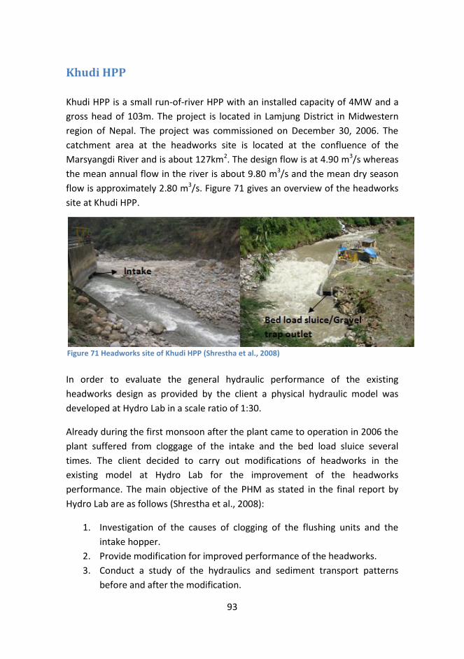
93
Khudi HPP
Khudi HPP is a small run-of-river HPP with an installed capacity of 4MW and a
gross head of 103m. The project is located in Lamjung District in Midwestern
region of Nepal. The project was commissioned on December 30, 2006. The
catchment area at the headworks site is located at the confluence of the
Marsyangdi River and is about 127km2. The design flow is at 4.90 m3/s whereas
the mean annual flow in the river is about 9.80 m3/s and the mean dry season
flow is approximately 2.80 m3/s. Figure 71 gives an overview of the headworks
site at Khudi HPP.
In order to evaluate the general hydraulic performance of the existing
headworks design as provided by the client a physical hydraulic model was
developed at Hydro Lab in a scale ratio of 1:30.
Already during the first monsoon after the plant came to operation in 2006 the
plant suffered from cloggage of the intake and the bed load sluice several
times. The client decided to carry out modifications of headworks in the
existing model at Hydro Lab for the improvement of the headworks
performance. The main objective of the PHM as stated in the final report by
Hydro Lab are as follows (Shrestha et al., 2008):
1. Investigation of the causes of clogging of the flushing units and the
intake hopper.
2. Provide modification for improved performance of the headworks.
3. Conduct a study of the hydraulics and sediment transport patterns
before and after the modification.
Figure 71 Headworks site of Khudi HPP (Shrestha et al., 2008)

94
4. Check the flushing ability of the bed load sluice.
5. Verify the abstraction of design discharge through the intake.
6. Recommend operational procedures for improved operation and
maintenance of the plant.
The salient features of the initial arrangement have been presented in
Appendix… and have not been further discussed in this section as it is the
functionalities the case study focuses on and not on the structural design itself.
The case study is specially relevant for understanding methods of sediment
handling and removal with respect to bed control and sediment passage at the
intake. The left and the right riverbank are differentiated while looking
downstream along the flow direction.
The initial arrangement
Figure 72 shows the PHM of the initial arrangement of the headworks area of
Khudi HPP. Clogging of the bed load flushing culvert was experienced at four
different occasions during the first monsoon operation of the plant. The
clogging of the bed load sluice and bed load hopper eventually led to an
increase in bed level in front of the semi-frontal intake due to sediment entry
into the gravel traps causing blockage of the entire intake. Very large logs and
boulders up to 0.62m was reported to be removed manually from the gravel
trap area (Shrestha et al., 2008).
Figure 72 PHM of the headworks of Khud HPP (Shrestha et al., 2008)

95
Several flows were tested on the model; both moderate flows and floods. The
bed load characteristics and the flow patterns were studied in order to identify
the factors responsible for intake blockage. Based on the tests performed
nearly 2/3 of the bed load sluice was observed to be under pressurization
during an average monsoon flood (80.0 m3/s) even in the absence of flow
contribution from the connected gravel trap. The pressurization length varied
with the extent of sediment concentration in the sluice. The pressurized flow
along the bed load sluice decreased the flow velocity causing sediment
deposition in the sluiceway.
Similarly, deposition was observed downstream of the bed load sluice that
extended upwards, suggesting insufficient flushing head in the sluice.
Pressurized flow in the bed load sluice was also enhanced by the entry of big
boulders in the sluice. Entry of smaller boulders and further interlocking also
induced further deposition. For a particular flow the performance of the bed
load decreased with an increase in sediment concentration it is, therefore, also
suggested that the bed load sluice blockage might also be a result of
unexpected amount of sediment inflow during flood.
Downstream river morphology also seemed to have an impact on the flushing
efficiency as there was no elevation drop in the river up to nearly a stretch of
about 20m from the bed load sluice outlet. Thus, deposition downstream
extended upwards to the bed load sluice and the hopper. The upstream flow of
the bed load sluice was also found to be disturbed by the mixing of the gravel
flushing flow connected with the bed load sluice as depositions were observed
upstream of the mixing point due to reduce velocities in this area.
Modifications adopted for the final arrangement
Following modifications were then adopted based on tests to eliminate the
above mentioned factors that were identified to be problematic:
1. Crest height increased to 1.5 m to a length of 3.0 m , curved with a radius of
4m, starting with the trash removal section to increase the flushing head of
the bed load sluice and create a stilling effect in the intake area decreasing
sediment inflow to the intake.

96
The overall width of the hopper was reduced at its starting point, joined to
the opening of the bed load sluice, by 3m with a side curve at the left bank.
The opening of the bed load sluice was reduced from the right most part to
have a net opening of 1.45m, in order to increase suction and decrease
sediment inflow into the bed load sluice. This helped to maintain the
sediment load within the flushing capacity of the culvert downstream
without flow pressurization. Furthermore, the gates were proportionally
increased with an increase in the flow and operated as needed.
A new Intake flood wall was raised to an elevation of 947.00 masl adjusted
at an angle with the initial flood wall end meeting tangentially to the curve
wall at the left bank. A hood of one and a half meter width was introduced
above the intake orifice top level to an elevation of the weir crest at 943.00
masl.
2. The gravel trap flushing canal was separated from the bed load sluice by
setting it parallel to the bed load sluice canal and was also extended further
downstream the bed load sluice to a length of 6.5m making an angle of 10
degrees to the river side with a slope of 1:50. The modification was meant
to eliminate the flow disturbances due to mixing.
Figure 73 Modifications at the intake of PHM of Khudi HPP (Shrestha et al., 2008)
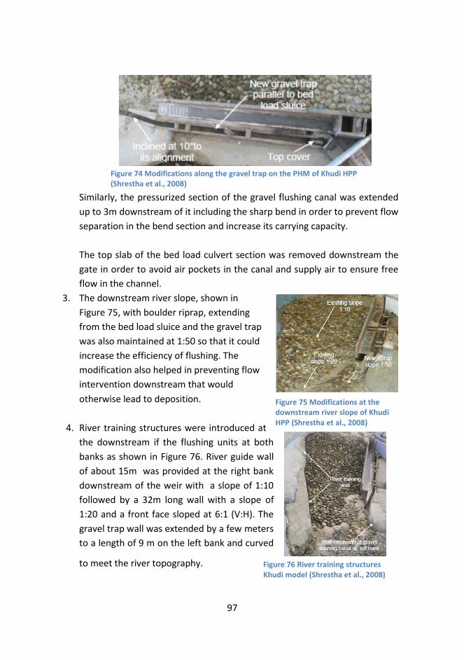
97
Similarly, the pressurized section of the gravel flushing canal was extended
up to 3m downstream of it including the sharp bend in order to prevent flow
separation in the bend section and increase its carrying capacity.
The top slab of the bed load culvert section was removed downstream the
gate in order to avoid air pockets in the canal and supply air to ensure free
flow in the channel.
3. The downstream river slope, shown in
Figure 75, with boulder riprap, extending
from the bed load sluice and the gravel trap
was also maintained at 1:50 so that it could
increase the efficiency of flushing. The
modification also helped in preventing flow
intervention downstream that would
otherwise lead to deposition.
4. River training structures were introduced at
the downstream if the flushing units at both
banks as shown in Figure 76. River guide wall
of about 15m was provided at the right bank
downstream of the weir with a slope of 1:10
followed by a 32m long wall with a slope of
1:20 and a front face sloped at 6:1 (V:H). The
gravel trap wall was extended by a few meters
to a length of 9 m on the left bank and curved
to meet the river topography.
Figure 74 Modifications along the gravel trap on the PHM of Khudi HPP (Shrestha et al., 2008)
Figure 75 Modifications at the downstream river slope of Khudi HPP (Shrestha et al., 2008)
Figure 76 River training structures Khudi model (Shrestha et al., 2008)

98
5. Sediment load reduction towards the
intake was achieved by introducing a
curve at the right bank upstream of
the weir with a top elevation of 944.0
masl. A curve wall also provided at the
left bank upstream of the weir axis
with top elevation at 945.0 masl
extending to the intake side wall. The
curve provided an outer bend towards
the intake reducing sediment load to
the intake. A normal flow towards the
intake was also secured to prevent the inflow of boulders during flood. The
modifications are illustrated in Figure 77.
Effects and Evaluation of the modifications
Flow channelization downstream of the
weir by separating the two flushing units
to overcome the downstream deposition
alone was found insufficient to increase
the performance of the headworks.
Increase in flushing head of the bed load
sluice due to weir increment increased
the stilling effect in front of the intake
with an increased sediment diversion
away from the intake and only
movement of fine sediments towards the
intake. The flushing capacity was
immensely improved. However,
turbulence was observed in front of the
intake leading to increased flow trash and floating debris towards the intake.
Curved river guide walls and diagonal weir installed upstream of the weir axis
helped decrease the sediment load towards the intake. The removal of the top
slab of bed load culvert section downstream of the gate and reduction of the
bed load opening aided in bed load flushing. The sediment concentration used
in the model were realized to be much more than reality and in consultation
Figure 78 Final arrangement of the PHM of Khudi HPP
Figure 77 River training structures at the intake of PHM of Khudi HPP (Shrestha et al., 2008)
99
with the client and the design consultant the sediment load was reduced to one
third of the concentration applied previously. The operation of the bed load
sluice gate was proportionally increased with the flow as sediment load
towards the intake increased with increase in the openings of the flushing unit.
Similarly, the gravel flushing was operated as required. The adopted solutions
were satisfactory for passage of sediments and sediment removal from the
intake. Turbulence in front of the intake was still existent.
A wall was added downstream of the weir axis to obtain smooth flow
downstream of the flushing units. Structures were installed in front of the
intake in variable numbers and of different shapes; however, these only
intensified the vortices in between them, and was proved unsatisfactory. Hood
above the intake with varying length from half a meter to two was used to
induce pressurization at the intake reducing velocity. This increased suction
from the bed load sluice, however the turbulence remained. Hopper size was
also reduced. This reduced sediment inflow to the intake and a continuous
suction was observed in the hopper with less deposition at the bed load sluice
suction area. Vortex was reduced to normal rotational flow with occasional
formation of suction vortex.
Trashes and debris were accumulated near the intake area due to reduction in
suction capacity of the vortex. Provision of the hood at the intake orifice top
level and a new positioning of the flood wall helped to remove trashes and
sediments more efficiently. Operation of the gravel trap had to be done with a
minimum possible opening of the bed load sluice. As the increased flushing
capability and sediment diversion lead to vortex formations at the intake
creating problem with trash and debris passage; the final design (Figure 78) of
the intake structure is a compromise between trash removal and bed load
removal in the headworks.

100
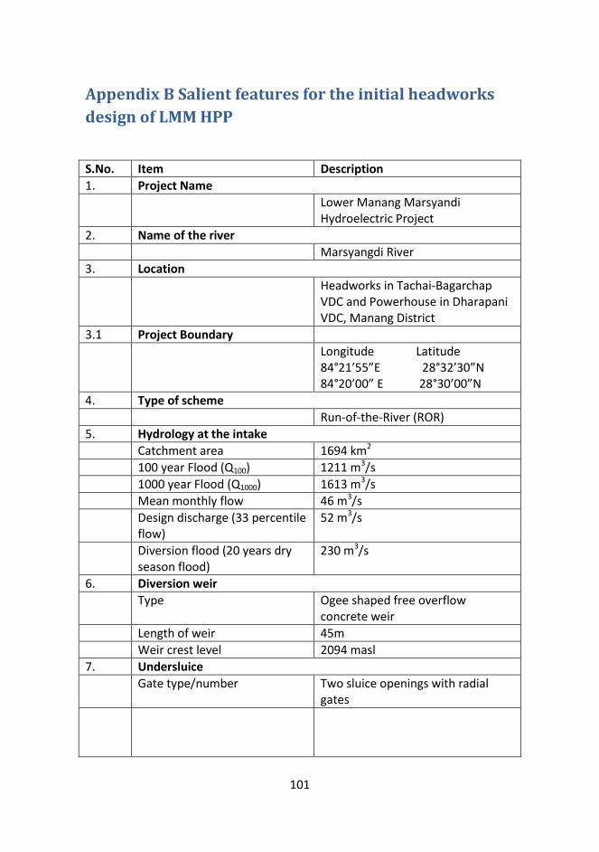
101
Appendix B Salient features for the initial headworks
design of LMM HPP
S.No. Item Description
1. Project Name
Lower Manang Marsyandi Hydroelectric Project
2. Name of the river
Marsyangdi River
3. Location
Headworks in Tachai-Bagarchap VDC and Powerhouse in Dharapani VDC, Manang District
3.1 Project Boundary
Longitude Latitude 84°21’55”E 28°32’30”N 84°20’00” E 28°30’00”N
4. Type of scheme
Run-of-the-River (ROR)
5. Hydrology at the intake
Catchment area 1694 km2
100 year Flood (Q100) 1211 m3/s
1000 year Flood (Q1000) 1613 m3/s
Mean monthly flow 46 m3/s
Design discharge (33 percentile flow)
52 m3/s
Diversion flood (20 years dry season flood)
230 m3/s
6. Diversion weir
Type Ogee shaped free overflow concrete weir
Length of weir 45m
Weir crest level 2094 masl
7. Undersluice
Gate type/number Two sluice openings with radial gates

102
Size of gates 4.5m wide and 9m high radial gate on the weir side 4.5m wide and 6.5m high radial gate with 2.5m high flap gate on top on the intake side
8. Intake
Type Side
Number and size Four side intakes 8.15m wide and 4m high
9. Gravel trap
Number Two
Size 9.5m long and 9.6m wide and 6.6 m deep from the normal operating level
Gravel flushing culvert 78.5m and 50m long culverts 1.5m wide and 1.5m high
10. Settling basin
Type Surface settling basin
Number Four basin with one hopper in each basin
Length 160 m
Width 8.2m
Height 8.3m at the start section, 10.3 m at the mid section and 12.3m at the end section including 2.85m deep hopper
Invert slope 1:40
Flushing Conventional gravity flushing
Flushing culvert size 2.5m wide and 2m deep
11. Power and energy output
Gross head 323m
Rated net head 311.1m
Installed capacity 138.41 MW
Gross Annual energy 675.54 GWh
Net dry season energy 77.96 GWh
Net wet season energy 568.04 GWh
Net annual estimated energy after deducting outage
646.00 GWh

103
Appendix C Velocity distributions along various Cross-Sections (CS)
CS2 CS3 CS4
CS6
CS5
CS5 CS6

104

105
12 Appendix D Plan layout of the final design of LMM
160.0 m
Bed load hopper
Pressurized sections Settling basins
Boulder Riprap
Dam weir
Gravel trap
Intake
Plan layout