Design of graph filters and filterbanks

HAL Id: hal-01675375https://hal.inria.fr/hal-01675375

Submitted on 4 Jan 2018

HAL is a multi-disciplinary open accessarchive for the deposit and dissemination of sci-entific research documents, whether they are pub-lished or not. The documents may come fromteaching and research institutions in France orabroad, or from public or private research centers.

L’archive ouverte pluridisciplinaire HAL, estdestinée au dépôt et à la diffusion de documentsscientifiques de niveau recherche, publiés ou non,émanant des établissements d’enseignement et derecherche français ou étrangers, des laboratoirespublics ou privés.

Design of graph filters and filterbanksNicolas Tremblay, Paulo Gonçalves, Pierre Borgnat

To cite this version:Nicolas Tremblay, Paulo Gonçalves, Pierre Borgnat. Design of graph filters and filterbanks. Petar M.Djurić; Cédric Richard. Cooperative and Graph Signal Processing, Academic Press, pp.299-324, 2018,978-0-12-813677-5. �10.1016/B978-0-12-813677-5.00011-0�. �hal-01675375�

https://hal.inria.fr/hal-01675375

https://hal.archives-ouvertes.fr

ii

“Book” — 2017/12/22 — 9:45 — page 1 — #1 ii

ii

ii

Design of graph filters andfilterbanks

Nicolas Tremblay,a,∗, Paulo Goncalvesa,∗∗ and Pierre Borgnata,†

∗Univ. Grenoble Alpes, CNRS, GIPSA-lab, Grenoble, France∗∗Universite Lyon, ENS de Lyon, Univ Lyon 1, CNRS, Inria, LIP & IXXI, Lyon, France

†Universite Lyon, ENS de Lyon, Univ Lyon 1, CNRS, Laboratoire de Physique & IXXI, Lyon, FranceaCorresponding: [email protected],

[email protected],

[email protected]

CHAPTER OUTLINE HEAD

1.1. Graph Fourier Transform and Frequencies . . . . . . . . . . . . . . . 5

1.1.1. Introduction . . . . . . . . . . . . . . . . . . . . . . . . . . . . . . 5

1.1.2. Graph Fourier Transform . . . . . . . . . . . . . . . . . . . . . . . 5

1.1.3. Frequencies of graph signals . . . . . . . . . . . . . . . . . . . . 9

1.1.4. Implementation and illustration . . . . . . . . . . . . . . . . . . . 11

1.2. Graph filters . . . . . . . . . . . . . . . . . . . . . . . . . . . . . . . . . 13

1.2.1. Definition of graph filters . . . . . . . . . . . . . . . . . . . . . . . 13

1.2.2. Properties of graph filters . . . . . . . . . . . . . . . . . . . . . . 15

1.2.3. Some designs of graph filters . . . . . . . . . . . . . . . . . . . . 16

1.2.4. Implementations of graph filters . . . . . . . . . . . . . . . . . . . 18

1.3. Filterbanks and multiscale transforms on graphs . . . . . . . . . . . 21

1.3.1. Continuous multi-scale transforms . . . . . . . . . . . . . . . . . 21

1.3.2. Discrete multi-scale transforms . . . . . . . . . . . . . . . . . . . 22

ABSTRACTBasic operations in graph signal processing consist in processing signals indexed on graphs ei-ther by filtering them or by changing their domain of representation, in order to better extractor analyze the important information they contain. The aim of this chapter is to review general

1

ii

“Book” — 2017/12/22 — 9:45 — page 2 — #2 ii

ii

ii

2 Design of graph filters and filterbanks

concepts underlying such filters and representations of graph signals. We first recall the dif-ferent Graph Fourier Transforms that have been developed in the literature, and show how tointroduce a notion of frequency analysis for graph signals by looking at their variations. Then,we move to the introduction of graph filters, that are defined like the classical equivalent for1D signals or 2D images, as linear systems which operate on each frequency of a signal. Someexamples of filters and of their implementations are given. Finally, as alternate representationsof graph signals, we focus on multiscale transforms that are defined from filters. Continuousmultiscale transforms such as spectral wavelets on graphs are reviewed, as well as the versatileapproaches of filterbanks on graphs. Several variants of graph filterbanks are discussed, forstructured as well as arbitrary graphs, with a focus on the central point of the choice of thedecimation or aggregation operators.

Keywords: graph signal processing, graph filters, filterbanks, wavelets, multi-resolution

0.1 GRAPH FOURIER TRANSFORM ANDFREQUENCIES

0.1.1 INTRODUCTIONGraph Signal Processing (GSP) has been introduced in the recent past using at leasttwo complementary formalisms: on the one hand, the discrete signal processingon graphs [1] (see also Chapter II.1) which emphasizes the adjacency matrix as ashift operator on graphs and develops an equivalent of Discrete Signal Processing(DSP) for signals on graphs; and on the other hand, the approaches rooted in graphspectral analysis, which rely on the spectral properties of a Laplacian matrix on agraph [2, 3, 4]. Both approaches yield a harmonic analysis of graph signals viathe definition of a Graph Fourier Transform : an operator projecting signals in thespectral domain of the chosen matrix. While the technical details vary, and someinterpretations in the vertex domain may differ, the fundamental objective of bothapproaches is to decompose a signal onto components of different frequencies andto design filters that can extract or modify parts of a graph signal according to thesefrequencies, e.g. providing notions of low-pass, band-pass, or high-pass filters forgraph signals. In this section, both approaches (along with other variations) are seenas specific instances of a general guideline for defining Graph Fourier Transform andits associated frequency analysis.

Notations.Vectors are written in bold with small letters, and matrices in bold and capital letters.Let G = (V,E,A) be a graph with V the set of N nodes, E the set of edges, and Athe weighted adjacency matrix in RN×N . If Ai j = 0, there is no connection from node

ii

“Book” — 2017/12/22 — 9:45 — page 3 — #3 ii

ii

ii

0.1 Graph Fourier Transform and Frequencies 3

i to node j, otherwise, Ai j is the weight of the edge starting from i and pointing1 to j.If an undirected edge exists between i and j, then Ai j = A ji. We restrict ourselves toadjacency matrices with positive or null entries: Ai j ≥ 0. Also, the symbol I denotesthe identity matrix (its dimension should be clear with the context), and δi is a vectorwhose i-th entry is equal to 1 while all other entries are equal to 0. Finally, we willdenote by |E| the number of edges in the graph.

0.1.2 GRAPH FOURIER TRANSFORMDefinition 1 (graph signal). A graph signal is a vector x ∈ RN whose component xi

is considered to be defined on vertex i.

A Graph Fourier Transform (GFT) is defined via a choice of reference operator2

admitting a spectral decomposition. Representing a graph signal in this spectraldomain is interpreted as a GFT. We review the standard properties and the variousdefinitions proposed in the literature.

Consider a matrix R ∈ RN×N . To be admissible as a reference operator for thegraph, it is often required that for any pair of nodes i , j, Ri j and R j i are equal tozero if i and j are not connected, as this will help for efficient implementations offilters (see Section 0.2.4). We assume furthermore that R is diagonalizable in C.In fact, if R is not diagonalizable, one needs to consider Jordan’s decomposition,which is out-of-scope of this chapter. We refer the reader to [1] and Chapter II.1 fortechnical details on how to handle this case. Nevertheless, in practice, we claim thatit often suffices to consider only diagonalizable operators, since: i) diagonalizablematrices in C are dense in the space of matrices; and ii) graphs under considerationare generally measured (should they model social, sensor or biological networks,...)with some inherent noise. Thus, if one ends up unluckily with a non-diagonalizablematrix, a small perturbation within the noise level will make it diagonalizable – pro-vided the graphs have no specific regularities that need to be kept. Still, we mayassume with only a small loss of generality that the reference operator R has a spec-tral decomposition:

R = UΛU−1, (0.1)

with U and Λ in CN×N . The columns of U, denoted as uk, are the right eigenvectorsof R, while the rows of U−1, denoted as v>k , are its left eigenvectors. Λ is the diagonalmatrix of the eigenvalues {λk}. The GFT is defined as the transformation of a graphsignal from the canonical “node” basis to its representation in the eigenvector basis:

1 In the literature, the converse convention is sometimes chosen (e.g. in [1]), hence the A> occasionallyappearing in this chapter.2 In the literature, this reference operator is often noted S for ”shift”. Nevertheless, the shift interpreta-tion is essentially valid if one considers S to be the adjacency matrix (see discussion in Section 0.2.1).In a general setting, we prefer to denote by R the reference operator.

ii

“Book” — 2017/12/22 — 9:45 — page 4 — #4 ii

ii

ii


Definition 2 (Graph Fourier Transform). For a given diagonalizable reference oper-ator R = UΛU−1 associated with a graph G, the GFT of a graph signal x ∈ RN is:

FG x .= x .

= U−1x. (0.2)

The GFT’s coefficients are simply the projections on the left eigenvectors of R:

∀k = 1, . . . ,N(FG x

)k = xk = vT

k x. (0.3)

Moreover, the GFT is invertible: U x = UU−1x = x. While, in general, the complexFourier modes uk are not orthogonal to each other, when R is symmetric, the follow-ing additional properties hold true.

The special case of symmetric reference operators. If in addition to be real, R isalso symmetric, then U and Λ are real matrices, and U may be found orthonormal,that is: U−1 = U>. In this case, vk = uk, the GFT of x is simply x = U>x withcoefficients xk = u>k x, and the Parseval relation holds: ||x||2 = ||x||2. Hereafter, whena symmetric operator R is encountered, one should have these properties in mind.

Finally, the interpretation of the graph Fourier modes uk in terms of oscillationsand frequencies will be the scope of Section 0.1.3. In the following, we list possiblechoices of reference operators, all diagonalizable with different U and Λ, thus alldefining different possible GFTs.

GFT for undirected graphsUndirected graphs are characterized by symmetric adjacency matrices: ∀(i, j) Ai j =

A j i. This does not necessarily mean that R has to be chosen symmetric as well, aswe will see with the example R = Lrw. The following choices of R are the mostcommon in the undirected case.

The combinatorial Laplacian [symmetric]. The first choice for R, advocated in[2, 3, 4] is to use the graph’s combinatorial Laplacian, having properties studied in[5]. It is defined as L = D − A where D is the diagonal matrix of nodes’ strengths,defined as Dii = di =

∑j Ai j. If the adjacency matrix is binary (i.e., unweighted), this

strength reduces to the degree of each node. The advantages of using L are twofold.i) It is an intuitive manner to define the GFT: L being the discretized version of thecontinuous Laplacian operator which admits the Fourier modes as eigenmodes, itis fair to use by analogy the eigenvectors of L as graph Fourier modes. Moreover,this choice is associated with a complete theory of vector calculus (e.g., gradients)for graph signals [6] that is useful to solve partial differential equations on graphs.ii) L has well known mathematical properties [5], giving ways to characterize thegraph or functions and processes on the graph (see also [7]). Most prominently, it issemi-definite positive (SDP) and its eigenvalues, being all positive or null, will servein the following to bind eigenvectors with a notion of frequency.

ii

“Book” — 2017/12/22 — 9:45 — page 5 — #5 ii

ii

ii


The normalized Laplacian [symmetric]. A second choice for R is the normalizedLaplacian Ln = D− 1

2 LD− 12 = I − D− 1

2 AD− 12 . An interesting property of this choice

of Laplacian is that all its eigenvalues lie between 0 and 2 [5].

The adjacency matrix, or deformed Laplacian [symmetric]. Another choicefor R is the adjacency matrix3 A>, as advocated in [1]. One readily sees that theeigenbasis U of A> and the eigenbasis of the deformed Laplacian Ld = I − A>

||A||2 ,where ||.||2 is the operator 2-norm, are the same. Therefore, the corresponding GFTsare equivalent and, for consistency in the presentation, we will use R = Ld here.

The random walk Laplacian [not symmetric]. The random walk Laplacian is yetanother Laplacian reading: Lrw = D−1L = I − D−1A, where D−1A serves also to de-scribe a uniform random walk on the graph. Even though Lrw is not symmetric, weknow it is diagonalizable in R. In fact, if uk is an eigenvector of Ln with eigenvalueλk, then D− 1

2 uk is an eigenvector of Lrw with same eigenvalue. Thus, Lrw has thesame eigenvalues as Ln, and its Fourier basis U is real but not orthonormal.

Other possible definitions of the reference operator. For instance, the consensusoperator (of the form I − σL with some suitable σ) [8], a geometric Laplacian [9],or some other deformed Laplacian one may think of, are valid alternatives.

All these operators imply a different spectral domain (different U and Λ) and, pro-vided one has a nice frequency interpretation (which is the object of Section 0.1.3),they all define possible GFTs. In the graph signal processing literature, the first threeoperators (L, Ln and Ld) are the most widely used.

GFT for directed graphsFor directed graphs, the adjacency matrix is no longer symmetric – Ai j is not neces-sarily equal to A j i – which does not automatically imply that the reference operatorR is not symmetric (e.g., the case R = Q below). This case is of great interest insome applications where the graph is naturally directed such as hyperlink graphs(there is a directed edge between website i and website j if there is a hyperlink inwebsite i directing to j). In directed graphs, the degree of node i is separated in itsout-degree, dout =

∑j Ai j, and its in-degree, din =

∑j A ji.

Some straightforward approaches [not symmetric]. It is possible to readily trans-pose the previous notions to the directed case, choosing either Dout or Din to replaceD in the different formulations: e.g. L = Din − A> as in [10], Lrw = I − Dout

−1A asin [11], Ln = I − Dout

− 12 ADout

− 12 . A notable choice is to directly use Ld = I − A>

||A||2

3 We use A> instead of A for consistency purposes with [1], whose convention for directed edges inthe adjacency matrix is converse to ours: what they call A is what we call A>. Without any influencein the undirected case, it has an impact in the directed case.

ii

“Book” — 2017/12/22 — 9:45 — page 6 — #6 ii

ii

ii


as in [1] (we recall that Ld and R = A> are equivalent for they share the sameeigenvectors and thus, define the same GFT). These matrices are no longer strictlyspeaking Laplacians as they are no longer SDP, but one may nonetheless considerthem as reference operators defining possible GFTs. Note that these definitionsentail to choose (rather arbitrarily) either Dout or Din in their formulations, with thenotable exception of Ld. In fact, Ld naturally generalizes to the directed case and isa classical choice of R in this context [1].

Chung’s directed Laplacian [symmetric]. A less common approach in the graphsignal processing community is the one provided by the directed Laplacians intro-duced by Chung [12]. To define these Laplacians, let us first introduce the randomwalk transition matrix (or operator) defined as P = D−1

outA. It admits a stationaryprobability4 π ∈ RN

+ such that π>P = π>. Writing Π = diag(π), Chung defines thefollowing two directed Laplacians:

Q = Π −ΠP + P>Π

2, (0.4)

Qn = Π−12 QΠ−

12 = I −

Π12 PΠ− 1

2 +Π−12 P>Π 1

2

2. (0.5)

Both the combinatorial Q and the normalized Qn directed Laplacians verify theproperties of Laplacian matrices: SDP, negative (or null) entries everywhere excepton the diagonal and real symmetric. It is easy to see that (0.4) and (0.5) generalizethe definitions of the undirected case since for an undirected graph,Π = D,ΠP = A;hence Q is the combinatorial Laplacian L, and Qn is its normalized version Ln.

Other possible definitions of the reference operator. The previous definitions ofLrw and Ld for undirected graphs may also be generalized to the directed Laplacianframework to obtain:

Qrw = I −P +Π−1P>Π

2and Qd = I −

ΠP + P>Π||ΠP + P>Π||2

. (0.6)

Additional notes. Other GFTs for directed graphs were proposed via the HermitianLaplacian as introduced in [13], which generalizes A>. A very different approachis to construct a Graph Fourier basis directly from an optimization scheme, requir-ing some notion of smoothness, or generalization of it – see [14, 15]. We will notconsider this recent approach here.

0.1.3 FREQUENCIES OF GRAPH SIGNALSTo complement the notion of GFT, one needs to introduce some frequency analysisof the Fourier modes on the graph. The general way of doing so is to compute how

4 Assuming the random walk is ergodic, i.e. irreducible and non-periodic.

ii

“Book” — 2017/12/22 — 9:45 — page 7 — #7 ii

ii

ii


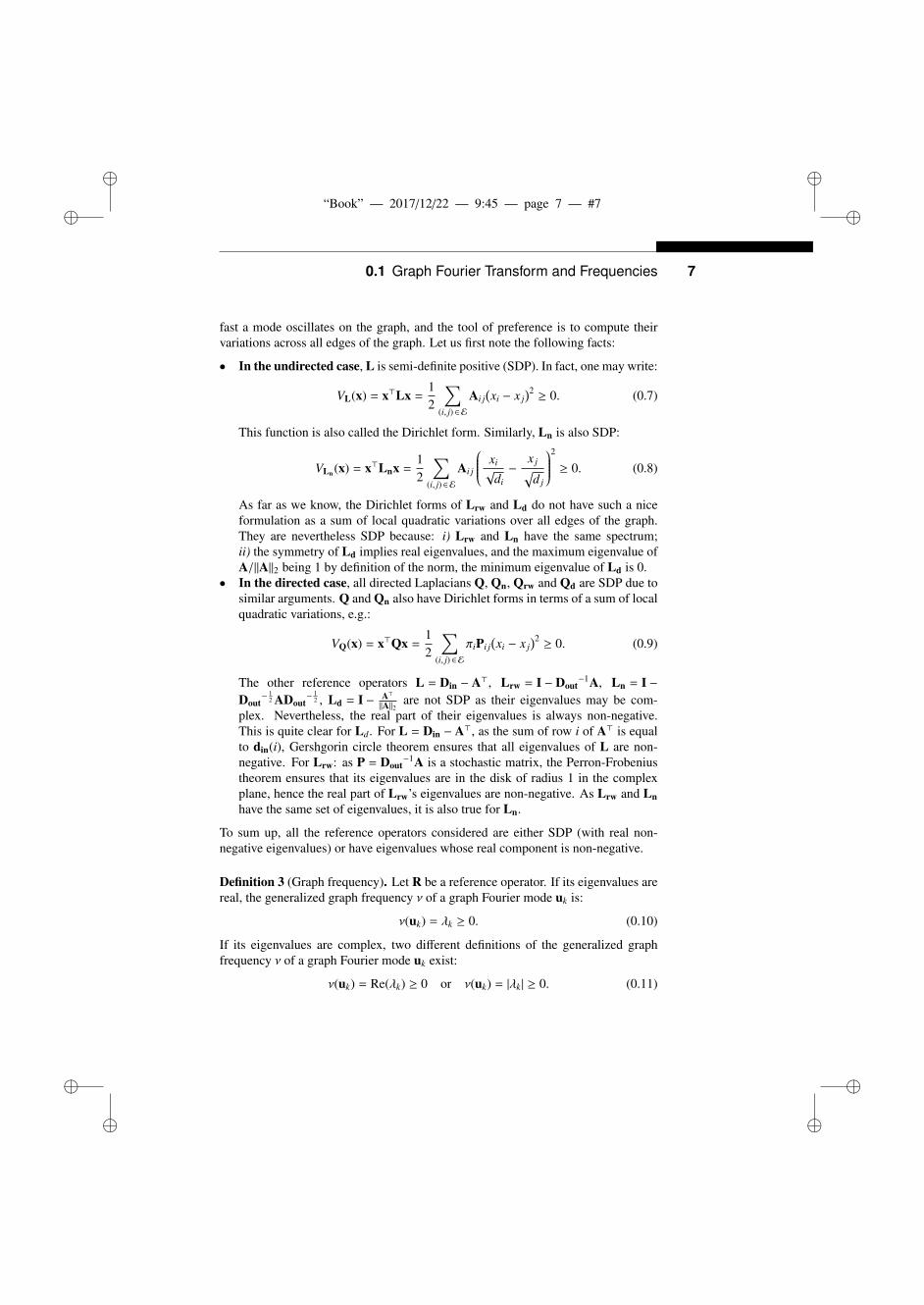
fast a mode oscillates on the graph, and the tool of preference is to compute theirvariations across all edges of the graph. Let us first note the following facts:

• In the undirected case, L is semi-definite positive (SDP). In fact, one may write:

VL(x) = x>Lx =12

∑(i, j) ∈E

Ai j(xi − x j

)2≥ 0. (0.7)

This function is also called the Dirichlet form. Similarly, Ln is also SDP:

VLn (x) = x>Lnx =12

∑(i, j) ∈E

Ai j

xi√

di−

x j√d j

2

≥ 0. (0.8)

As far as we know, the Dirichlet forms of Lrw and Ld do not have such a niceformulation as a sum of local quadratic variations over all edges of the graph.They are nevertheless SDP because: i) Lrw and Ln have the same spectrum;ii) the symmetry of Ld implies real eigenvalues, and the maximum eigenvalue ofA/||A||2 being 1 by definition of the norm, the minimum eigenvalue of Ld is 0.

• In the directed case, all directed Laplacians Q, Qn, Qrw and Qd are SDP due tosimilar arguments. Q and Qn also have Dirichlet forms in terms of a sum of localquadratic variations, e.g.:

VQ(x) = x>Qx =12

∑(i, j) ∈E

πiPi j(xi − x j

)2≥ 0. (0.9)

The other reference operators L = Din − A>, Lrw = I − Dout−1A, Ln = I −

Dout− 1

2 ADout− 1

2 , Ld = I − A>||A||2 are not SDP as their eigenvalues may be com-

plex. Nevertheless, the real part of their eigenvalues is always non-negative.This is quite clear for Ld. For L = Din − A>, as the sum of row i of A> is equalto din(i), Gershgorin circle theorem ensures that all eigenvalues of L are non-negative. For Lrw: as P = Dout

−1A is a stochastic matrix, the Perron-Frobeniustheorem ensures that its eigenvalues are in the disk of radius 1 in the complexplane, hence the real part of Lrw’s eigenvalues are non-negative. As Lrw and Lnhave the same set of eigenvalues, it is also true for Ln.

To sum up, all the reference operators considered are either SDP (with real non-negative eigenvalues) or have eigenvalues whose real component is non-negative.

Definition 3 (Graph frequency). Let R be a reference operator. If its eigenvalues arereal, the generalized graph frequency ν of a graph Fourier mode uk is:

ν(uk) = λk ≥ 0. (0.10)

If its eigenvalues are complex, two different definitions of the generalized graphfrequency ν of a graph Fourier mode uk exist:

ν(uk) = Re(λk) ≥ 0 or ν(uk) = |λk | ≥ 0. (0.11)

ii

“Book” — 2017/12/22 — 9:45 — page 8 — #8 ii

ii

ii


Remarks. In the case of complex eigenvalues, it is a matter of choice whether weconsider the imaginary part of the eigenvalues or not. There is no current consensuson this question. A second remark deals with the case of a multiple eigenvalueλk, i.e., if there are several eigenvectors associated to the same λk; then, only onefrequency ν(λk) is defined for the associated eigenspace.

Justification: the link between frequency and variation. Two types of variationmeasures have been considered in the literature to show the consistency betweenthis definition of graph frequencies and a notion of oscillation over the graph. Thefirst one is based on the quadratic forms of the Laplacian operators. For instance,in the undirected case with the combinatorial Laplacian, Eq. (0.7) applied to anynormalized Fourier mode uk defined from L reads:

VL(uk) = u>k Luk =12

∑(i, j) ∈E

Ai j(uk(i) − uk( j)

)2= λk ||uk ||

22 = λk. (0.12)

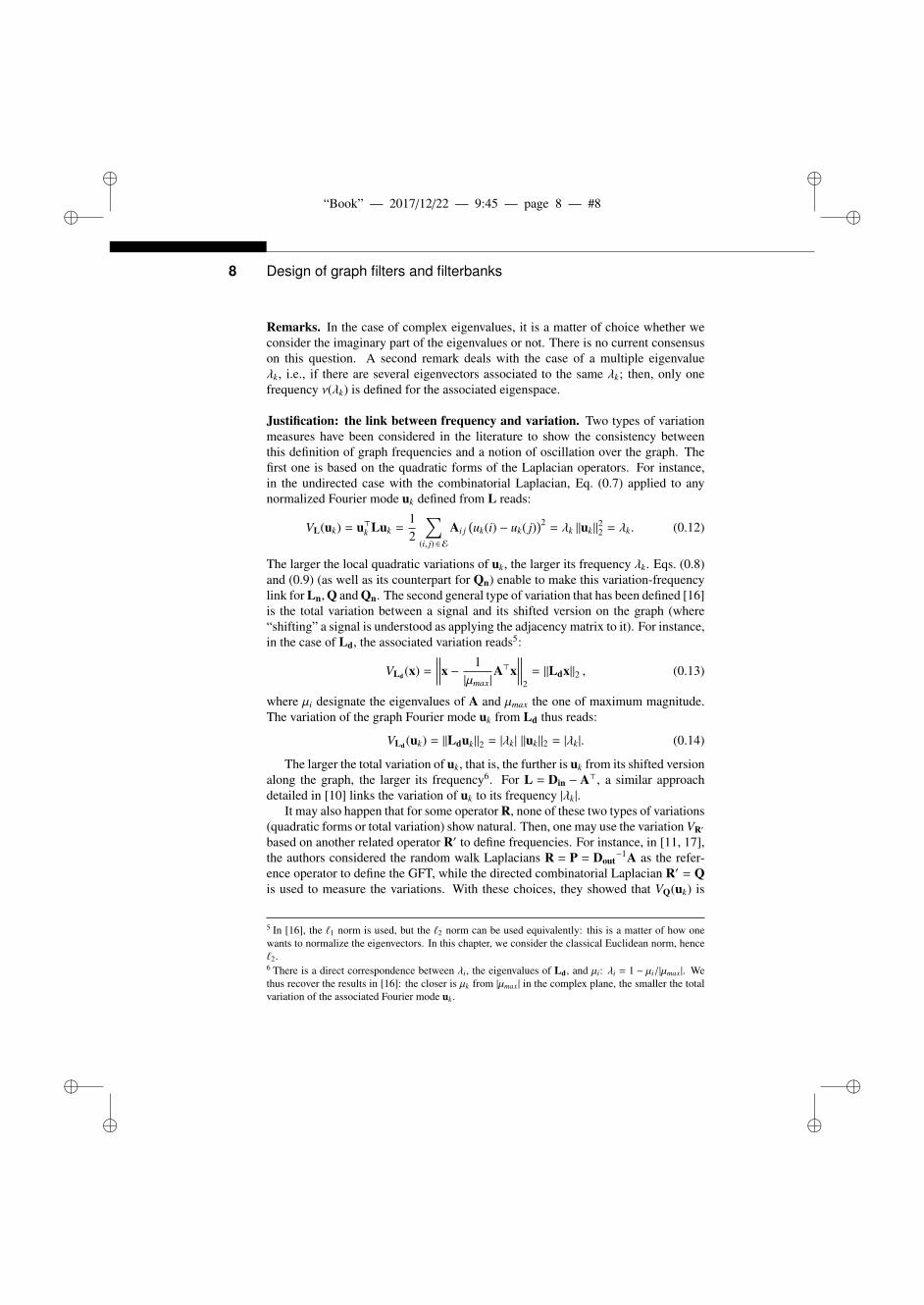
The larger the local quadratic variations of uk, the larger its frequency λk. Eqs. (0.8)and (0.9) (as well as its counterpart for Qn) enable to make this variation-frequencylink for Ln,Q and Qn. The second general type of variation that has been defined [16]is the total variation between a signal and its shifted version on the graph (where“shifting” a signal is understood as applying the adjacency matrix to it). For instance,in the case of Ld, the associated variation reads5:

VLd (x) =

∣∣∣∣∣∣∣∣∣∣x − 1|µmax|

A>x∣∣∣∣∣∣∣∣∣∣

2= ||Ldx||2 , (0.13)

where µi designate the eigenvalues of A and µmax the one of maximum magnitude.The variation of the graph Fourier mode uk from Ld thus reads:

VLd (uk) = ||Lduk ||2 = |λk | ||uk ||2 = |λk |. (0.14)

The larger the total variation of uk, that is, the further is uk from its shifted versionalong the graph, the larger its frequency6. For L = Din − A>, a similar approachdetailed in [10] links the variation of uk to its frequency |λk |.

It may also happen that for some operator R, none of these two types of variations(quadratic forms or total variation) show natural. Then, one may use the variation VR′

based on another related operator R′ to define frequencies. For instance, in [11, 17],the authors considered the random walk Laplacians R = P = Dout

−1A as the refer-ence operator to define the GFT, while the directed combinatorial Laplacian R′ = Qis used to measure the variations. With these choices, they showed that VQ(uk) is

5 In [16], the `1 norm is used, but the `2 norm can be used equivalently: this is a matter of how onewants to normalize the eigenvectors. In this chapter, we consider the classical Euclidean norm, hence`2.6 There is a direct correspondence between λi, the eigenvalues of Ld, and µi: λi = 1 − µi/|µmax |. Wethus recover the results in [16]: the closer is µk from |µmax | in the complex plane, the smaller the totalvariation of the associated Fourier mode uk.

ii

“Book” — 2017/12/22 — 9:45 — page 9 — #9 ii

ii

ii


a) -0.4

-0.2

0

0.2

0.4

b) -0.4

-0.2

0

0.2

0.4

c)0 0.5 1

0

0.5

1L

Ln

Ld

d)0 0.5 1

0

0.1

0.2L

Ln

Ld

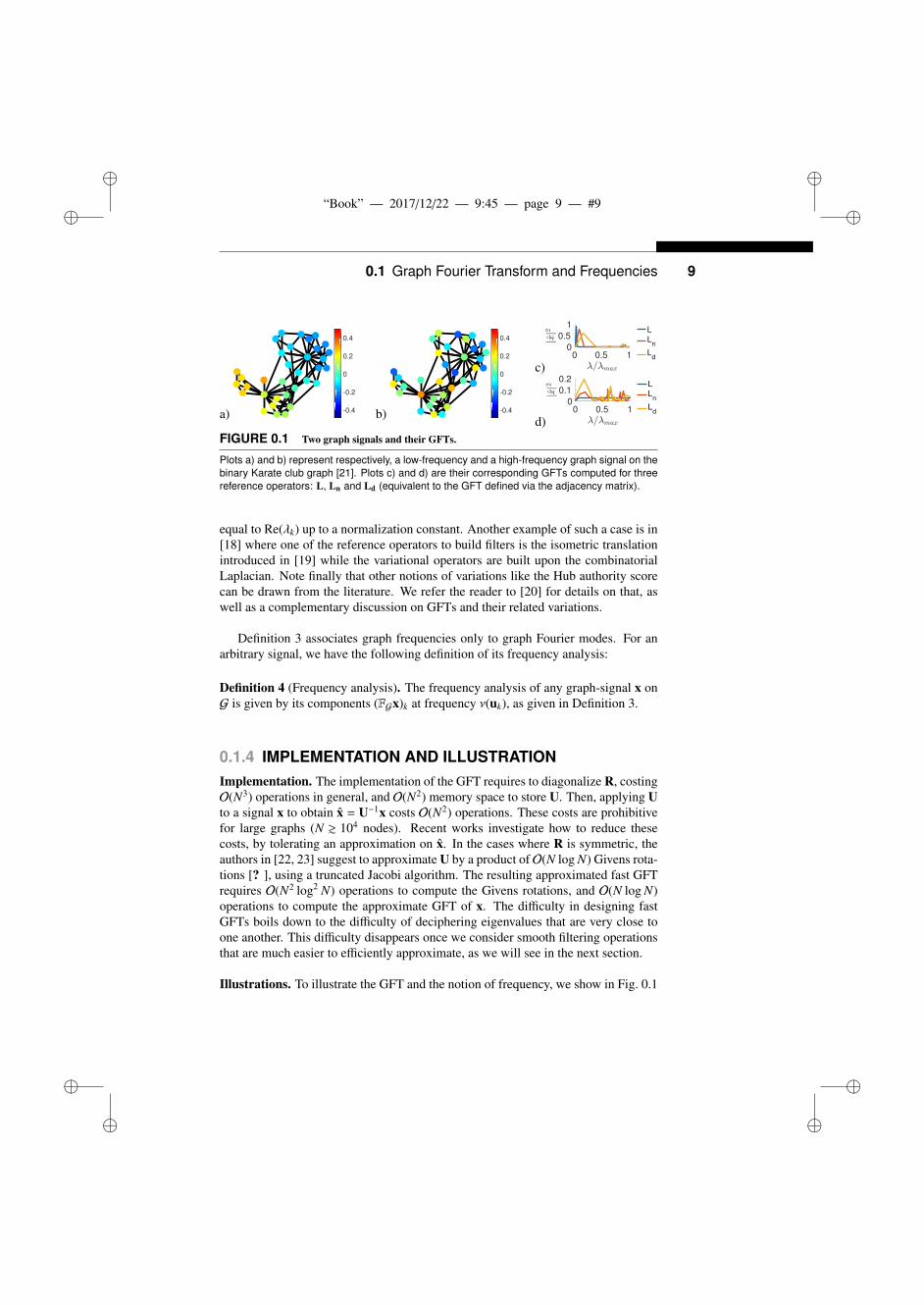
FIGURE 0.1 Two graph signals and their GFTs.

Plots a) and b) represent respectively, a low-frequency and a high-frequency graph signal on thebinary Karate club graph [21]. Plots c) and d) are their corresponding GFTs computed for threereference operators: L, Ln and Ld (equivalent to the GFT defined via the adjacency matrix).

equal to Re(λk) up to a normalization constant. Another example of such a case is in[18] where one of the reference operators to build filters is the isometric translationintroduced in [19] while the variational operators are built upon the combinatorialLaplacian. Note finally that other notions of variations like the Hub authority scorecan be drawn from the literature. We refer the reader to [20] for details on that, aswell as a complementary discussion on GFTs and their related variations.

Definition 3 associates graph frequencies only to graph Fourier modes. For anarbitrary signal, we have the following definition of its frequency analysis:

Definition 4 (Frequency analysis). The frequency analysis of any graph-signal x onG is given by its components (FGx)k at frequency ν(uk), as given in Definition 3.

0.1.4 IMPLEMENTATION AND ILLUSTRATIONImplementation. The implementation of the GFT requires to diagonalize R, costingO(N3) operations in general, and O(N2) memory space to store U. Then, applying Uto a signal x to obtain x = U−1x costs O(N2) operations. These costs are prohibitivefor large graphs (N & 104 nodes). Recent works investigate how to reduce thesecosts, by tolerating an approximation on x. In the cases where R is symmetric, theauthors in [22, 23] suggest to approximate U by a product of O(N log N) Givens rota-tions [? ], using a truncated Jacobi algorithm. The resulting approximated fast GFTrequires O(N2 log2 N) operations to compute the Givens rotations, and O(N log N)operations to compute the approximate GFT of x. The difficulty in designing fastGFTs boils down to the difficulty of deciphering eigenvalues that are very close toone another. This difficulty disappears once we consider smooth filtering operationsthat are much easier to efficiently approximate, as we will see in the next section.

Illustrations. To illustrate the GFT and the notion of frequency, we show in Fig. 0.1

ii

“Book” — 2017/12/22 — 9:45 — page 10 — #10 ii

ii

ii


a) -0.4

-0.2

0

0.2

0.4

ω

b)0 0.5 1

0

0.5

1

=0

=2

=4

=10

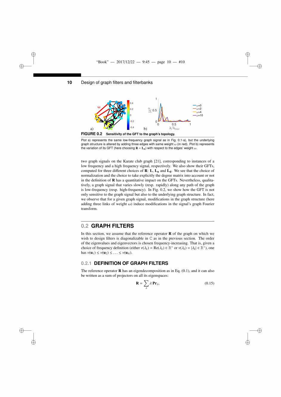
FIGURE 0.2 Sensitivity of the GFT to the graph’s topology.

Plot a) represents the same low-frequency graph signal as in Fig. 0.1-a), but the underlyinggraph structure is altered by adding three edges with same weight ω (in red). Plot b) representsthe variation of its GFT (here choosing R = Ln) with respect to the edges’ weight ω.

two graph signals on the Karate club graph [21], corresponding to instances of alow frequency and a high frequency signal, respectively. We also show their GFTs,computed for three different choices of R: L, Ln and Ld. We see that the choice ofnormalization and the choice to take explicitly the degree matrix into account or notin the definition of R has a quantitative impact on the GFTs. Nevertheless, qualita-tively, a graph signal that varies slowly (resp. rapidly) along any path of the graphis low-frequency (resp. high-frequency). In Fig. 0.2, we show how the GFT is notonly sensitive to the graph signal but also to the underlying graph structure. In fact,we observe that for a given graph signal, modifications in the graph structure (hereadding three links of weight ω) induce modifications in the signal’s graph Fouriertransform.

0.2 GRAPH FILTERSIn this section, we assume that the reference operator R of the graph on which wewish to design filters is diagonalizable in C as in the previous section. The orderof the eigenvalues and eigenvectors is chosen frequency-increasing. That is, given achoice of frequency definition (either ν(λk) = Re(λk) ∈ R+ or ν(λk) = |λk | ∈ R

+), onehas ν(u1) ≤ ν(u2) ≤ . . . ≤ ν(uN).

0.2.1 DEFINITION OF GRAPH FILTERSThe reference operator R has an eigendecomposition as in Eq. (0.1), and it can alsobe written as a sum of projectors on all its eigenspaces:

R =∑λ

λ Prλ, (0.15)

ii

“Book” — 2017/12/22 — 9:45 — page 11 — #11 ii

ii

ii

0.2 Graph filters 11

where the sum is on all different eigenvalues λ and Prλ is the projector on theeigenspace associated with eigenvalue λ, i.e.:

Prλ =∑λk=λ

ukv>k .

Definition 5 (wide-sense definition of a graph filter). The most general definition ofa graph filter is an operator that acts separately on all the eigenspaces of R, dependingon their eigenvalue λ. Mathematically, any function

h : C→ R (0.16)λ→ h(λ). (0.17)

defines a graph filter H such that

H =∑λ

h(λ) Prλ =∑

k

h(λk)ukv>k . (0.18)

To each eigenspace of R with eigenvalue λ is associated a filtering weight h(λ)that attenuates or increases the importance of this eigenspace in the decompositionof the signal of interest. In fact, one may write the action of H on a signal x as:

Hx =∑λ

h(λ) Prλ x. (0.19)

For any function g, let us write g(Λ) as a shorthand notation for diag(g(λ1) . . . , g(λN)).A graph filter can be written as:

H = U h(Λ) U−1. (0.20)

Using functional calculus of operators, this is equivalently written as H = h(R),which calls for some interpretation remarks. In fact, this expression opens the wayto interpret what is the action of a graph filter in the vertex domain. Firstly, note thatapplying R to a graph signal is in fact a local computation on the graph: on eachnode, the resulting transformed signal is a weighted sum of the values of the originalsignal on its (direct) neighbours. Therefore, in the node space, a filter H = h(R) canbe interpreted as an operator that weights the information on the signal transmittedthrough edges of the graph, the same way classical filters are built on the basic oper-ation of time-shift. This fundamental analogy shift/reference operator was first madein [1] and explains why in the GSP literature, reference operators are often called”shift operators”.

Now, to illustrate the notion of graph filtering in the spectral domain, considerthe graph signal x =

∑k αkuk and y = Hx. The k-th Fourier component of x being,

by construction, xk = v>k x = αk, its filtered version reads:

y = Hx =∑

k

h(λk)αkuk. (0.21)

ii

“Book” — 2017/12/22 — 9:45 — page 12 — #12 ii

ii

ii


Hence the k-th Fourier component of the filtered signal is yk = h(λk)αk, recalling theclassical interpretation of filtering as a multiplication in the Fourier domain. We callh(λ) the frequency response of the filter.

In many cases, it is more convenient and natural to restrict ourselves to functionsh that associate the same real number to all values of λ ∈ {λ s.t. ν(λ) = ν ∈ R+}. Thatis, considering any two eigenvalues λ1 and λ2 associated with the same frequencyν(λ1) = ν(λ2), we restrict ourselves to functions h such that h(λ1) = h(λ2). This en-tails the following narrowed-sense definition of a graph filter.

Definition 6 (narrowed-sense definition of a graph filter). Any function

h : R+ → R (0.22)ν→ h(ν). (0.23)

defines a narrowed-sense graph filter H such that

H =∑λ

h(ν(λ)) Prλ = Uh(v(Λ))U−1. (0.24)

Remark. If the eigenvalues are real, both definitions 5 and 6 are equivalent sinceν(λ) = λ ∈ R+.

Examples of narrowed-sense filters:

• The constant filter equal to c: h(ν) = c. In this case, h(ν(Λ)) = cI and H = cI: allfrequencies are allowed to pass, and no component is filtered out.

• The Kronecker delta in ν∗: h(ν) = δν,ν∗ . If there exists one (or several) eigenvaluesλ of R such that ν(λ) = ν∗, then H =

∑λ s.t. ν(λ)=ν∗ Prλ. If not, then H = 0. For this

filter, only the frequency ν∗ is allowed to pass.• The ideal low-pass with cut-off frequency νc: h(ν) = 1 if ν ≤ νc, and 0 otherwise.

In this case: H =∑λ,s.t.ν(λ)≤νc

Prλ, i.e., only frequencies up to νc are allowed topass.

• The heat kernel h(ν) = exp−ν/ν0 : the weight associated with ν is exponentiallydecreasing with the frequency ν. Actually y = H x0 is the solution of the graphdiffusion (or heat) equation (see [2]) at time t = 1/ν0 with initial condition x0.

0.2.2 PROPERTIES OF GRAPH FILTERSFrom now on, in order to simplify notations and concepts in this introductory chapteron graph filtering, we will restrict ourselves to symmetric reference operators, suchas L, Ln, or Ld in the undirected case, or the directed Laplacians Q or Qn in thedirected case. In this case, the eigenvalues are real such that the frequency defini-tion is straightforward ν(λ) = λ, both filter definitions are equivalent such that the

ii

“Book” — 2017/12/22 — 9:45 — page 13 — #13 ii

ii

ii


frequency response reads

h : R+ → R (0.25)λ→ h(λ), (0.26)

and one may find a real orthonormal graph Fourier basis U such that U−1 = U>. Afiltering operator associated with h thereby reads:

H = Uh(Λ)U> ∈ RN×N . (0.27)

All results presented in the following may be (carefully) generalized to the unsym-metric case.

Definition 7. We write Cp the set of finite-order polynomials in R:

Cp =

H s.t. H =

n∑i=0

aiRi, {ai}i=0,...,n ∈ Rn+1, n ∈ N\{+∞}

. (0.28)

Proposition 1. Cp is equal to the set of graph filters.

Proof. Consider H ∈ Cp. Then, defining h(λ) =∑n

i=0 aiλi, one has: H =

∑ni=0 aiRi =

U∑n

i=0 aiΛiU> = Uh(Λ)U>, i.e., H is a filter. Now, consider H a filter, i.e., there

exists h such that H = Uh(Λ)U>. Consider the polynomial∑N−1

i=0 aiλi that interpo-

lates through all pairs (λi, h(λi)). The maximum degree of such a polynomial isN − 1 as there are maximum N points to interpolate, and may be smaller if eigen-values have multiplicity larger than one. Thereby, one may write: H = Uh(Λ)U> =

U∑N−1

i=0 aiΛiU> =

∑N−1i=0 aiRi. Writing n = N − 1, this means that H ∈ Cp. �

Consequence: An equivalent definition of a graph filter is a polynomial in R.

Definition 8. We write Cd the set of all diagonal operators in the graph Fourier space:

Cd = {H, s.t. U>HU is diagonal}. (0.29)

Proposition 2. The set of graph filters is included in Cd. Both sets are equal iff alleigenspaces of R are simple (i.e., all eigenvalues are of multiplicity one).

Proof. By definition of graph filters, they are included in Cd. Now, in general, anelement of Cd is not necessarily a graph filter. In fact, given H ∈ Cd, all diagonalentries of U>HU may be chosen independently, which is not the case for the diagonalentries of h(Λ) corresponding to the same eigenspace. Thus, both sets are equal iffall eigenspaces are of dimension one. �

Consequence: In the case where all eigenvalues are simple, an equivalent definition

ii

“Book” — 2017/12/22 — 9:45 — page 14 — #14 ii

ii

ii


of a graph filter is a diagonal matrix in the graph Fourier basis.

Definition 9. We write Cc the set of matrices that commute with R:

Cc = {H s.t. RH = HR}. (0.30)

Proposition 3. Cp ⊆ Cc. The equality holds iff all eigenvalues of R are simple.

Proof. A polynomial in R necessarily commutes with R, thus Cp ⊆ Cc. Now, ingeneral, an element in Cc is not necessarily in Cp. In fact, if H ∈ Cc, then ΛY = YΛwith Y = U>HU. Suppose Λ = λI. In this case, commutativity does not constrainY at all, thereby H is not necessarily in Cp. Now, if we suppose that all eigenvalueshave multiplicity one, i.e., all diagonal entries ofΛ are different, the only solution forY is to be a diagonal matrix, i.e., Cc = Cd. We showed in Prop. 2 that the set of graphfilters is equal to Cd iff all eigenvalues have multiplicity one, therefore: Cc = Cp iffall eigenvalues have multiplicity one. �

Consequence: In the case where all eigenvalues are simple, an equivalent definitionof a graph filter is a linear operator that commutes with R.

0.2.3 SOME DESIGNS OF GRAPH FILTERSFrom the previous sections, it should now be clear that the frequency response of afilter H only alters the frequencies ν(λ) corresponding to the discrete set of eigenval-ues of R (see Eq. (0.18)). More generally though, the frequency response of a graphfilter can be defined over a continuous range of λ’s, leading to the notion of universalfilter design, i.e. a filter whose frequency response h(λ) is designed for all λ’s and notonly adapted to the specific eigenvalues of R. On the contrary, a graph-dependentfilter design depends specifically on these eigenvalues.

FIR filters. From the results of Section 0.2.2, a natural class of graph filters isgiven in the form of Finite Impulse Response (FIR) filters, as by eq. (0.28) with apolynomial of finite order, which realizes a weighted Moving Average (MA) filteringof a signal. Also, one can design any universal filter by fitting the desired responseh(λ) with a polynomial

∑ni=0 aiλ

i. The larger n is, the closer the filter can approximatethe desired shape. If the approximation is done only using the h(λk), the design isgraph-dependent, else it is universal if fitting some function h(λ).

Let us then go back to the interpretation of R as a graph shift operator in thenode space, (as studied or recalled for instance in [1, 24, 29, 20]), and see how itoperates for FIR filters. Applied to a graph signal, the terms Ri in eq. (0.28), act as ai-hops local computation on the graph: on each node, the resulting filtered signal is aweighted sum of the values of the original signal lying in its i-th neighbourhood, thatis, nodes attainable with a path of length i along the graph. Then, like for classical

ii

“Book” — 2017/12/22 — 9:45 — page 15 — #15 ii

ii

ii


signals, FIR filters only imply a finite neighbourhood of each nodes, and this willtranslate in Section 0.2.4 into distributed, fast implementations of these filters. Still,FIR filters are usually poor at approximating filters with sharp changes of desiredfrequency response, as illustrated for instance in Fig. 1 of [24].

ARMA filters. A more versatile approximation of h(λ) can be obtained with a ratio-nal design [24, 25, 26]:

h(λ) =

∑qi=0 biλ

i

1 +∑p

i=1 aiλi=

pq(λ)pp(λ)

. (0.31)

Such a rational filter is called an Auto-Regressive Moving Average filter of order(p, q) and is commonly noted ARMA(p, q). Again, it is known from classical DSPthat an ARMA design, being a IIR (Infinite Impulse Response) filter, is more adapt-able at approximating various shapes of filters, especially with sharp changes in thefrequency response. The filtering relation y = Hx for ARMA filters can be written inthe node domain as: (1 +

∑pi=1 aiRi)y = (

∑qi=0 biRi)x. This ARMA filter expression

will lead to the distributed implementation, discussed later in 0.2.4. For instance, foran ARMA(1,0) (i.e., an AR(1)) one will have to use: y = −a1Ry + b0x.

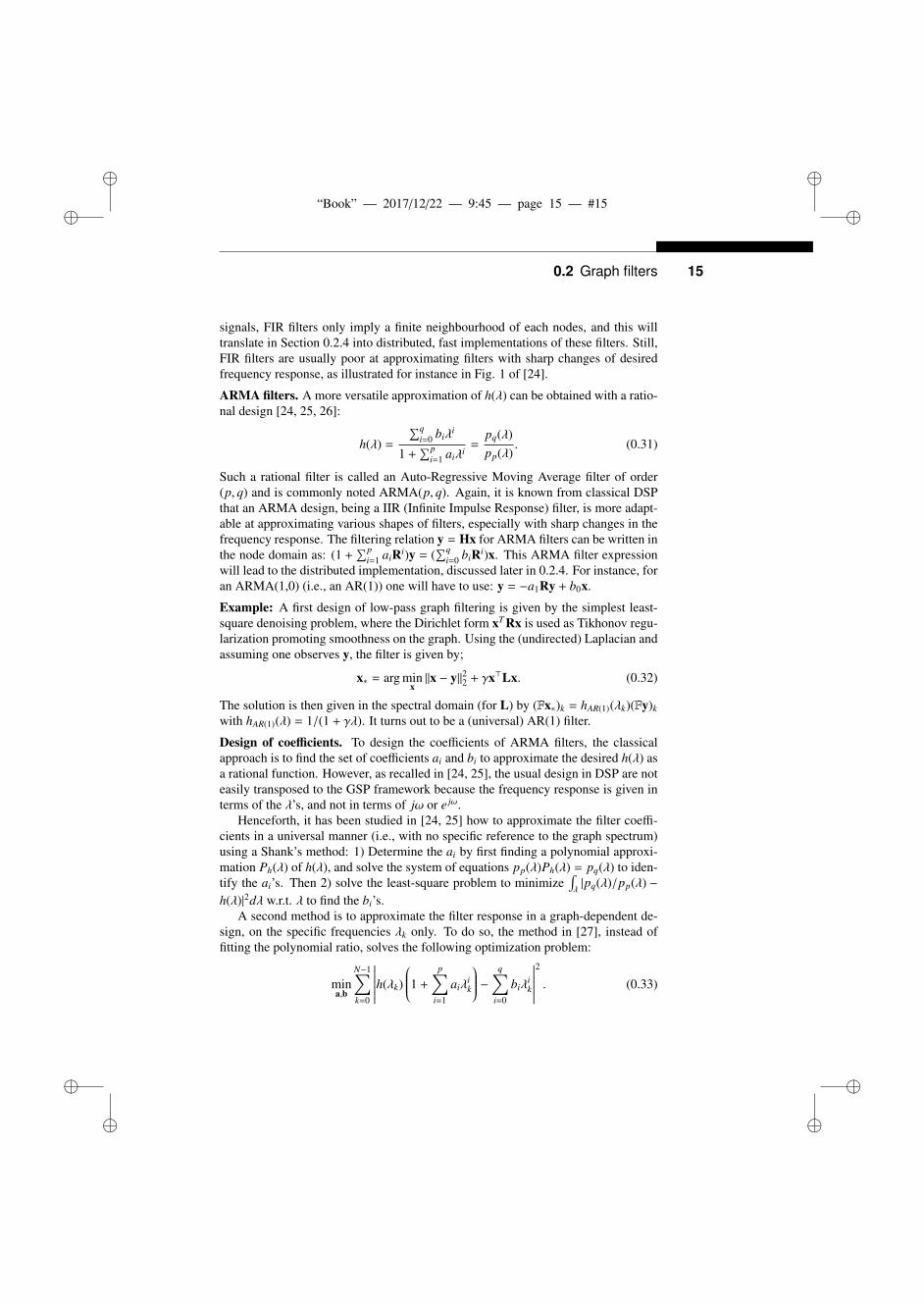
Example: A first design of low-pass graph filtering is given by the simplest least-square denoising problem, where the Dirichlet form xT Rx is used as Tikhonov regu-larization promoting smoothness on the graph. Using the (undirected) Laplacian andassuming one observes y, the filter is given by;

x∗ = arg minx||x − y||22 + γx>Lx. (0.32)

The solution is then given in the spectral domain (for L) by (Fx∗)k = hAR(1)(λk)(Fy)k

with hAR(1)(λ) = 1/(1 + γλ). It turns out to be a (universal) AR(1) filter.

Design of coefficients. To design the coefficients of ARMA filters, the classicalapproach is to find the set of coefficients ai and bi to approximate the desired h(λ) asa rational function. However, as recalled in [24, 25], the usual design in DSP are noteasily transposed to the GSP framework because the frequency response is given interms of the λ’s, and not in terms of jω or e jω.

Henceforth, it has been studied in [24, 25] how to approximate the filter coeffi-cients in a universal manner (i.e., with no specific reference to the graph spectrum)using a Shank’s method: 1) Determine the ai by first finding a polynomial approxi-mation Ph(λ) of h(λ), and solve the system of equations pp(λ)Ph(λ) = pq(λ) to iden-tify the ai’s. Then 2) solve the least-square problem to minimize

∫λ|pq(λ)/pp(λ) −

h(λ)|2dλ w.r.t. λ to find the bi’s.A second method is to approximate the filter response in a graph-dependent de-

sign, on the specific frequencies λk only. To do so, the method in [27], instead offitting the polynomial ratio, solves the following optimization problem:

mina,b

N−1∑k=0

∣∣∣∣∣∣∣h(λk)

1 +

p∑i=1

aiλik

− q∑i=0

biλik

∣∣∣∣∣∣∣2

. (0.33)

ii

“Book” — 2017/12/22 — 9:45 — page 16 — #16 ii

ii

ii


Using again a polynomial approximation Ph(λ), the solution derives from the leastsquare solution (see details in [27]).

AR filters to model random processes. We do not discuss much in this chapterrandom processes on graphs ; for that, see the framework to study stationary randomprocesses on graphs in [28, 29], and Chapter II.5. Still, a remark can be done for theparametric modeling of random processes. As introduced in [1], one can model aprocess on a graph as the output of a graph filter, generally taken as an ARMA filter.Here, we discuss the case of AR filters. The linear prediction is written as:

x =

p∑i=1

aiRix. (0.34)

The coefficients of this filter can directly be obtained by numerical inversion ofx = Ba where B = (Rx,R2x, . . . ,Rpx). The solution is given by the pseudo-inverse:a# = (B>B)−1B>x which minimizes the squared error ||x − Ba||22, w.r.t to a. Anotherpossibility would be to estimate the coefficients of the AR model by means of theorthogonality principle leading to the Yule-Walker (YW) equations, as follows:

E{(Rkx)>Rx)

}=

p∑i=1

aiE{(Rix)>Rkx

}= 0, (0.35)

Depending on the structure of the reference operator R, we have:

1. If R is symmetric (R> = R, as often for undirected graph), the autocorrelationfunction involved in this YW system is: ρx(m, n) = E

{(Rmx)>Rnx

}= γx(m + n);

2. When R is unitary (for instance with R as the isometric operator from [19]), thecorresponding autocorrelation will be ρx(m, n) = E

{(Rmx)>Rnx

}= γx(n − m) and

the usual techniques to solve the YW system can be used.

Experimentally, it was found that the isometric operator of [19] or a consensus oper-ator are the one that offer a more exact and stable modeling [18].

0.2.4 IMPLEMENTATIONS OF GRAPH FILTERSGiven a frequency response h, how to efficiently filter a graph signal x?

The direct approach. It consists in first diagonalizing R to obtain U and Λ; thencomputing the filter matrix H = Uh(Λ)U>; and finally left-multiplying the graphsignal x by H to obtain its filtered version. The overall computational cost of thisprocedure is O(N3) arithmetic operations due to the diagonalization and O(N2)memory space as the graph Fourier transform U is dense in general.

The polynomial approximate filtering approach. More efficiently though, we canfirst quickly estimate λmin and λmax (for instance via the power method) and second,look for a polynomial that best approximates h(λ) on the whole interval [λmin, λmax].

ii

“Book” — 2017/12/22 — 9:45 — page 17 — #17 ii

ii

ii


Let us call hi the coefficients of this approximate polynomial. We have:

Hx = Uh(Λ)U>x ' Up∑

i=0

hiΛiU>x =

p∑i=0

hiRix. (0.36)

The number of required arithmetic operations is O(p|E|), where p is a trade-off

between precision and computational cost. Also, the easier is h approachable by alow-order polynomial, the better the approximation. At the same time, the larger pis, the more accurate the approximation is. The authors of [30] recommend Cheby-chev polynomials as an approximation basis as they are known to be optimal in the∞-norm sense. In some circumstances, other choices can be preferred. For instance,when approximating the ideal low-pass, Chebychev polynomials yield Gibbs oscil-lations around the cut-off frequency that turn penalizing for smooth filters. In thatcase, other choices are possible [31], such as the Jackson-Chebychev polynomialsthat attenuate such unwanted oscillations.

The Lanczos approximate filtering approach. In [32], and based on works by [33],the authors propose an approximate filtering approach based on Lanczos iterations.Given a signal x, the Lanczos algorithm computes an orthonormal basis Vp ∈ R

N×p

of the Krylov subspace associated with x: Kp(L, x) = span(x,Lx, . . . ,Lp−1x), as wellas a small tridiagonal matrix Hp ∈ R

p×p such that: V∗pLVp = Hp. The approximatefiltering then reads:

Hx ' ||x||2Vph(Hp)δ1. (0.37)

At fixed p, this approach has a typical complexity in O(p|E|), possibly raised toO(p|E| + N p2) if a reorthonomalisation is needed to stabilize the algorithm; a costthat is comparable to that of the polynomial approximation approach. Theoretically,the quality of approximation is similar (see [32] for details). In practice however, ithas been observed that if the spectrum is regularly spaced, polynomial approxima-tions should be preferred, while the Lanczos method has an edge over others in thecase of irregularly-spaced spectra. This is understandable as Krylov subspaces arealso used for diagonalization purposes (see for instance, chapter 6 of [34]) and thusnaturally adapt to the underlying spectrum.

Distributed implementation of ARMA filters. The ARMA filters being definedthrough a rational fraction, are IIR filters. Henceforth, the polynomials approach todistribute and fasten the computation are not the most efficient ones. The methodsdeveloped in [25, 26] yield a distributed implementation of ARMA filters. The firstpoint is to remember that the rational filter of eq. (0.31) can be implemented fromits partial fraction decomposition as a sum of polynomial fractions of order 1 only.Then, the distributed implementation of filtering x can be done by studying the 1storder recursion [25]:

y(t + 1) = cMy(t) + dx (0.38)

ii

“Book” — 2017/12/22 — 9:45 — page 18 — #18 ii

ii

ii


-0.4

-0.2

0

0.2

0.4

-0.4

-0.2

0

0.2

0.4

-0.4

-0.2

0

0.2

0.4

-0.4

-0.2

0

0.2

0.4

noisy x

x = UTx^

^ ^xd = h(Λ) x

xd = Uh(Λ)UTx

xd = Uxd

denoised xd

node space

graph Fourier space

0 10 200

0.5

10 10 20

0

0.5

1

0 10 200

0.5

1

x = UTx^

^ ^xd = h(Λ) x

xd = Uxd

graph Fourier space

0 10 200

0.5

10 10 20

0

0.5

1

0 10 200

0.5

1

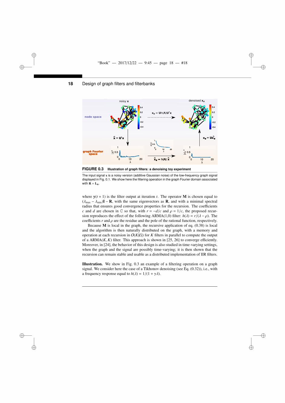
FIGURE 0.3 Illustration of graph filters: a denoising toy experiment

The input signal x is a noisy version (additive Gaussian noise) of the low-frequency graph signaldisplayed in Fig. 0.1. We show here the filtering operation in the graph Fourier domain associatedwith R = Ln.

where y(t + 1) is the filter output at iteration t. The operator M is chosen equal to(λmax − λmin)I − R, with the same eigenvectors as R, and with a minimal spectralradius that ensures good convergence properties for the recursion. The coefficientsc and d are chosen in C so that, with r = −d/c and ρ = 1/c, the proposed recur-sion reproduces the effect of the following ARMA(1,0) filter: h(λ) = r/(λ − ρ). Thecoefficients r and ρ are the residue and the pole of the rational function, respectively.

Because M is local in the graph, the recursive application of eq. (0.38) is localand the algorithm is then naturally distributed on the graph, with a memory andoperation at each recursion in O(K|E|) for K filters in parallel to compute the outputof a ARMA(K,K) filter. This approach is shown in [25, 26] to converge efficiently.Moreover, in [24], the behavior of this design is also studied in time-varying settings,when the graph and the signal are possibly time-varying; it is then shown that therecursion can remain stable and usable as a distributed implementation of IIR filters.

Illustration. We show in Fig. 0.3 an example of a filtering operation on a graphsignal. We consider here the case of a Tikhonov denoising (see Eq. (0.32)), i.e., witha frequency response equal to h(λ) = 1/(1 + γλ).

ii

“Book” — 2017/12/22 — 9:45 — page 19 — #19 ii

ii

ii

0.3 Filterbanks and multiscale transforms on graphs 19

0.3 FILTERBANKS AND MULTISCALETRANSFORMS ON GRAPHS

To process and filter signals on graphs, it is attractive to develop equivalent of mul-tiscale transforms such as wavelets, i.e. ways to decompose a graph signal on com-ponents at different scales, or frequency ranges. The road to multiscale transformson graphs has originally been tackled in the vertex domain [35] to analyze data onnetworks. Thereafter, a general design of multiscale transforms was based on thediffusion of signals on the graph structure, leading to the powerful framework ofDiffusion Wavelets [36, 37]. This latter works were already based on a diffusionoperators, usually a Laplacian or a random walk operator, whose powers are decom-posed in order to obtain a multiscale orthonormal basis. The objective was to builda kind of equivalent of discrete wavelet transforms for graph signals.

In this chapter, we focus on two other constructions of multiscale transforms ongraphs which are more related to the Graph Fourier Transform. The frequency anal-ysis and filters described here are: 1) the method of [3] which develops an analogof continuous wavelet transform on graphs, 2) approaches that combine filters ongraphs with graph decompositions through decimation (pioneered in [4] with deci-mation of bipartite graphs) or aggregation of nodes; in a nutshell, these methods arevery close to the filter banks implementation of discrete wavelets [38].

0.3.1 CONTINUOUS MULTI-SCALE TRANSFORMSIn the following, we work with undirected graphs and R = Ln = I − D− 1

2 AD− 12 ,

whose eigenvalues are contained in the interval [0, 2]. The generalization to otheroperators can be done using the guidelines of previous sections.

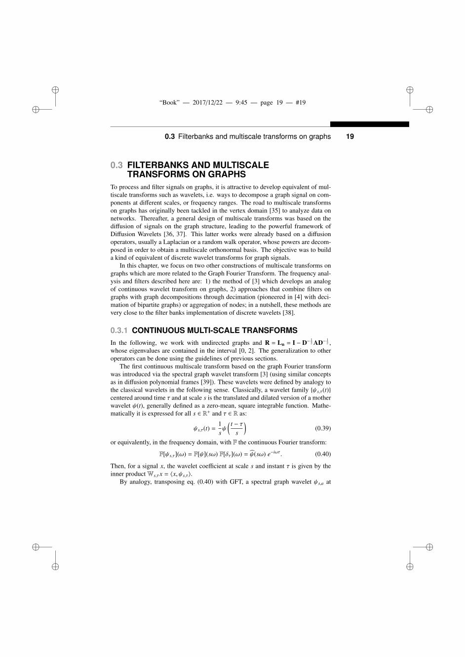
The first continuous multiscale transform based on the graph Fourier transformwas introduced via the spectral graph wavelet transform [3] (using similar conceptsas in diffusion polynomial frames [39]). These wavelets were defined by analogy tothe classical wavelets in the following sense. Classically, a wavelet family {ψs,τ(t)}centered around time τ and at scale s is the translated and dilated version of a motherwavelet ψ(t), generally defined as a zero-mean, square integrable function. Mathe-matically it is expressed for all s ∈ R+ and τ ∈ R as:

ψs,τ(t) =1sψ

( t − τs

)(0.39)

or equivalently, in the frequency domain, with F the continuous Fourier transform:

F[ψs,τ](ω) = F[ψ](sω) F[δτ](ω) = ψ(sω) e−iωτ. (0.40)

Then, for a signal x, the wavelet coefficient at scale s and instant τ is given by theinner productWs,τx = 〈x, ψs,τ〉.

By analogy, transposing eq. (0.40) with GFT, a spectral graph wavelet ψs,a at

ii

“Book” — 2017/12/22 — 9:45 — page 20 — #20 ii

ii

ii


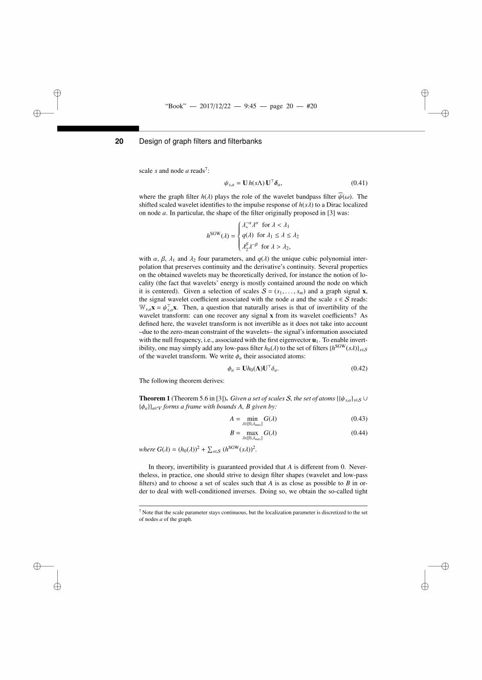
scale s and node a reads7:

ψs,a = U h(sΛ) U>δa, (0.41)

where the graph filter h(λ) plays the role of the wavelet bandpass filter ψ(ω). Theshifted scaled wavelet identifies to the impulse response of h(sλ) to a Dirac localizedon node a. In particular, the shape of the filter originally proposed in [3] was:

hSGW(λ) =

λ−α∗ λ

α for λ < λ1

q(λ) for λ1 ≤ λ ≤ λ2

λβ2λ−β for λ > λ2,

with α, β, λ1 and λ2 four parameters, and q(λ) the unique cubic polynomial inter-polation that preserves continuity and the derivative’s continuity. Several propertieson the obtained wavelets may be theoretically derived, for instance the notion of lo-cality (the fact that wavelets’ energy is mostly contained around the node on whichit is centered). Given a selection of scales S = (s1, . . . , sm) and a graph signal x,the signal wavelet coefficient associated with the node a and the scale s ∈ S reads:Ws,ax = ψ>s,ax. Then, a question that naturally arises is that of invertibility of thewavelet transform: can one recover any signal x from its wavelet coefficients? Asdefined here, the wavelet transform is not invertible as it does not take into account–due to the zero-mean constraint of the wavelets– the signal’s information associatedwith the null frequency, i.e., associated with the first eigenvector u1. To enable invert-ibility, one may simply add any low-pass filter h0(λ) to the set of filters {hSGW(sλ)}s∈Sof the wavelet transform. We write φa their associated atoms:

φa = Uh0(Λ)U>δa. (0.42)

The following theorem derives:

Theorem 1 (Theorem 5.6 in [3]). Given a set of scalesS, the set of atoms {{ψs,a}s∈S ∪

{φa}}a∈V forms a frame with bounds A, B given by:

A = minλ∈[0,λmax]

G(λ) (0.43)

B = maxλ∈[0,λmax]

G(λ) (0.44)

where G(λ) = (h0(λ))2 +∑

s∈S (hSGW(sλ))2.

In theory, invertibility is guaranteed provided that A is different from 0. Never-theless, in practice, one should strive to design filter shapes (wavelet and low-passfilters) and to choose a set of scales such that A is as close as possible to B in or-der to deal with well-conditioned inverses. Doing so, we obtain the so-called tight

7 Note that the scale parameter stays continuous, but the localization parameter is discretized to the setof nodes a of the graph.

ii

“Book” — 2017/12/22 — 9:45 — page 21 — #21 ii

ii

ii


(or snug) frames, i.e. frames such that A = B (or A ≈ B). An approach is to useclassical dyadic decompositions using bandlimited filters such as in Table 1 of [40].Another desirable property of such frames is their discriminatory power: the abilityat discerning different signals only by considering their wavelet coefficients. For afilterbank to be discriminative, each filter element needs to take into account infor-mation from a similar number of eigenvalues of the Laplacian. The eigenvalues of anarbitrary graph being unevenly spaced on [0, λmax], one needs to compute or estimatethe exact density of the spectrum of the graph under consideration [41].

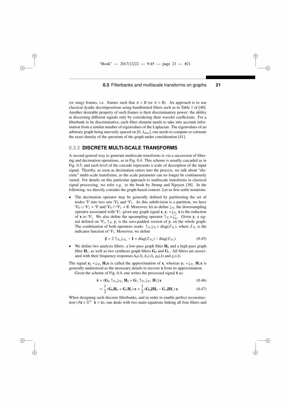
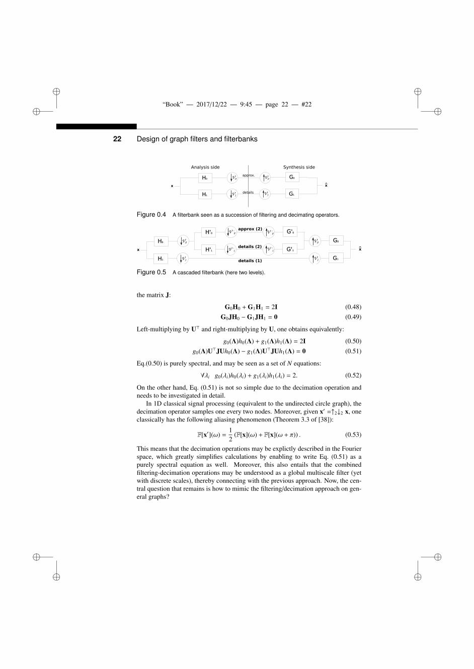
0.3.2 DISCRETE MULTI-SCALE TRANSFORMSA second general way to generate multiscale transforms is via a succession of filter-ing and decimation operations, as in Fig. 0.4. This scheme is usually cascaded as inFig. 0.5, and each level of the cascade represents a scale of description of the inputsignal. Thereby, as soon as decimation enters into the process, we talk about “dis-crete” multi-scale transforms, as the scale parameter can no longer be continuouslyvaried. For details on this particular approach to multiscale transforms in classicalsignal processing, we refer e.g. to the book by Strang and Nguyen [38]. In thefollowing, we directly consider the graph-based context. Let us first settle notations:

• The decimation operator may be generally defined by partitioning the set ofnodes V into two sets V0 and V1. As this subdivision is a partition, we haveV0 ∪V1 = V andV0 ∩V1 = ∅. Moreover, let us define ↓Vi the downsamplingoperator associated withVi: given any graph signal x, yi =↓Vi x is the reductionof x to Vi. We also define the upsampling operator ↑Vi=↓

>Vi

. Given yi a sig-nal defined on Vi, ↑Vi yi is the zero-padded version of yi on the whole graph.The combination of both operators reads: ↑Vi↓Vi= diag(IVi ), where IVi is theindicator function ofVi. Moreover, we define

J = 2 ↑V0↓V0 − I = diag(IV0 ) − diag(IV1 ). (0.45)

• We define two analysis filters: a low-pass graph filter H0 and a high-pass graphfilter H1, as well as two synthesis graph filters G0 and G1. All filters are associ-ated with their frequency responses h0(λ), h1(λ), g0(λ) and g1(λ).

The signal y0 =↓V0 H0x is called the approximation of x, whereas y1 =↓V1 H1x isgenerally understood as the necessary details to recover x from its approximation.

Given the scheme of Fig. 0.4, one writes the processed signal x as:

x =(G0 ↑V0↓V0 H0 + G1 ↑V1↓V1 H1

)x (0.46)

=12

(G0H0 + G1H1) x +12

(G0JH0 −G1JH1) x. (0.47)

When designing such discrete filterbanks, and in order to enable perfect reconstruc-tion (∀x ∈ RN x = x), one deals with two main equations linking all four filters and

ii

“Book” — 2017/12/22 — 9:45 — page 22 — #22 ii

ii

ii


H0

H1

G0

G1

x x

approx.

details

V0

Analysis side Synthesis side

V1

V0

V1

Figure 0.4 A filterbank seen as a succession of filtering and decimating operators.

H0

H1

G0

G1

x x

H'0

H'1

G'0

G'1

approx (2)

details (2)

details (1)

V0

V1

V0

V1

V '0

V '1

V '0

V '1

Figure 0.5 A cascaded filterbank (here two levels).

the matrix J:

G0H0 + G1H1 = 2I (0.48)G0JH0 −G1JH1 = 0 (0.49)

Left-multiplying by U> and right-multiplying by U, one obtains equivalently:

g0(Λ)h0(Λ) + g1(Λ)h1(Λ) = 2I (0.50)g0(Λ)U>JUh0(Λ) − g1(Λ)U>JUh1(Λ) = 0 (0.51)

Eq.(0.50) is purely spectral, and may be seen as a set of N equations:

∀λi g0(λi)h0(λi) + g1(λi)h1(λi) = 2. (0.52)

On the other hand, Eq. (0.51) is not so simple due to the decimation operation andneeds to be investigated in detail.

In 1D classical signal processing (equivalent to the undirected circle graph), thedecimation operator samples one every two nodes. Moreover, given x′ =↑2↓2 x, oneclassically has the following aliasing phenomenon (Theorem 3.3 of [38]):

F[x′](ω) =12

(F[x](ω) + F[x](ω + π)) . (0.53)

This means that the decimation operations may be explictly described in the Fourierspace, which greatly simplifies calculations by enabling to write Eq. (0.51) as apurely spectral equation as well. Moreover, this also entails that the combinedfiltering-decimation operations may be understood as a global multiscale filter (yetwith discrete scales), thereby connecting with the previous approach. Now, the cen-tral question that remains is how to mimic the filtering/decimation approach on gen-eral graphs?

ii

“Book” — 2017/12/22 — 9:45 — page 23 — #23 ii

ii

ii


In Section 0.3.2.1, it will be shown that for very well structured graphs such asbipartite graphs or m-cyclic graphs, generalizations of the decimation operator maybe defined and their effect explicitly described as graph filters. Then the case ofarbitrary graph is studied in 0.3.2.2 where the “one every two nodes” paradigm isnot transposable directly; several approaches to do that will then be reviewed.

0.3.2.1 Filterbanks on bipartite graphs and other stronglystructured graphs

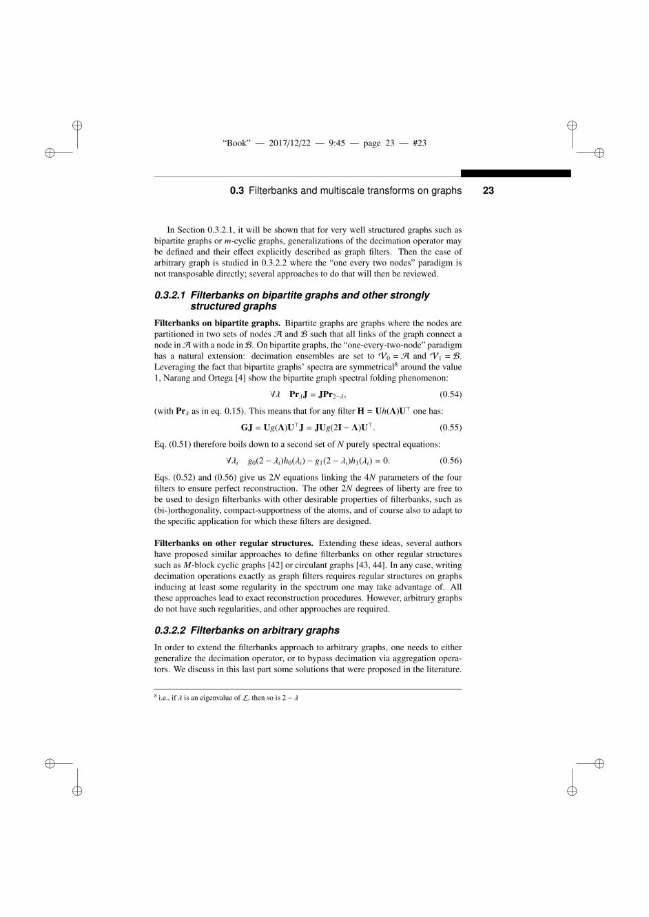
Filterbanks on bipartite graphs. Bipartite graphs are graphs where the nodes arepartitioned in two sets of nodes A and B such that all links of the graph connect anode inAwith a node inB. On bipartite graphs, the “one-every-two-node” paradigmhas a natural extension: decimation ensembles are set to V0 = A and V1 = B.Leveraging the fact that bipartite graphs’ spectra are symmetrical8 around the value1, Narang and Ortega [4] show the bipartite graph spectral folding phenomenon:

∀λ PrλJ = JPr2−λ, (0.54)

(with Prλ as in eq. 0.15). This means that for any filter H = Uh(Λ)U> one has:

GJ = Ug(Λ)U>J = JUg(2I − Λ)U>. (0.55)

Eq. (0.51) therefore boils down to a second set of N purely spectral equations:

∀λi g0(2 − λi)h0(λi) − g1(2 − λi)h1(λi) = 0. (0.56)

Eqs. (0.52) and (0.56) give us 2N equations linking the 4N parameters of the fourfilters to ensure perfect reconstruction. The other 2N degrees of liberty are free tobe used to design filterbanks with other desirable properties of filterbanks, such as(bi-)orthogonality, compact-supportness of the atoms, and of course also to adapt tothe specific application for which these filters are designed.

Filterbanks on other regular structures. Extending these ideas, several authorshave proposed similar approaches to define filterbanks on other regular structuressuch as M-block cyclic graphs [42] or circulant graphs [43, 44]. In any case, writingdecimation operations exactly as graph filters requires regular structures on graphsinducing at least some regularity in the spectrum one may take advantage of. Allthese approaches lead to exact reconstruction procedures. However, arbitrary graphsdo not have such regularities, and other approaches are required.

0.3.2.2 Filterbanks on arbitrary graphs

In order to extend the filterbanks approach to arbitrary graphs, one needs to eithergeneralize the decimation operator, or to bypass decimation via aggregation opera-tors. We discuss in this last part some solutions that were proposed in the literature.

8 i.e., if λ is an eigenvalue of L, then so is 2 − λ

ii

“Book” — 2017/12/22 — 9:45 — page 24 — #24 ii

ii

ii


A complementary and thoughtful discussion on graph decimation, graph aggregationand graph reconstruction can be found in sections III and IV of [45]. For that, thetwo key questions are:

• how to generalize the decimation operator on arbitrary graphs? We will see thatgeneralized decimation operators either try to mimic the classical decimation andattempt to sample “one every two nodes”, or aggregate nodes to form supernodesaccording in general to some graph cut objective function.

• how to build the new coarser-scale graph from the decimated nodes (or aggre-gated supernodes)? In fact, after each decimation, if one wants to cascade thefilterbank, a new coarse-grain graph has to be built in order to define the nextlevel’s graph filters. The nodes (resp. supernodes) are set thanks to decimation(resp. aggregation): but how do we link them together?

Graph decimation. The first work to generalize filterbanks on arbitrary graphs isdue to Narang and Ortega [4] and consists in decomposing the graph into an edge-disjoint collection of bipartite subgraphs, and then to apply the scheme presented inSection 0.3.2.1 on each of the subgraphs. In this collection, each subgraph has thesame node set, and the union of all subgraphs sums to the original graph. To per-form this decomposition (which is not unique), the same authors propose a coloring-based algorithm, called Harary’s decomposition. Sakiyama and Tanaka [46] alsoused this decomposition as one of their design’s cornerstone. Unsatisfied by the NP-completeness of the coloring problem (even though heuristics exist), Nguyen andDo [47] propose another decomposition method based on maximum spanning trees.

The bipartite paradigm’s main advantage comes from the fact that decimationhas an explicit formulation in the graph’s Fourier space, thereby enabling exactfilter designs depending on the given task. In our opinion, when applied to arbitrarygraphs, its main drawback comes from the non-unicity of the bipartite subgraphsdecomposition, as well as the seemingly arbitrariness of such a decomposition: froma graph signal point-of-view, what is the meaning of a bipartite decomposition?Letting go of this paradigm, and slightly changing the general filterbank design pre-sented in Section 0.3.2.1, other generalized graph decimations have been proposed.For instance, in [48], the authors propose to separate the graph in two sets V0,V1according to its max cut, i.e., maximizing

∑i∈V0

∑j∈V1

Wi j. In [45], the authorssuggest similarly to partition the graph into two sets according to the polarity of thelast eigenvector (i.e. the eigenvector associated with the highest frequency). In [49],the authors use an original approach based on random forests to sample nodes, wherethey have a probabilistic version of “equally-spaced” nodes on the graph.

Graph aggregation. Another paradigm in graph reduction is graph aggregation,where, instead of selecting nodes as in decimation, one aggregates entire regions ofthe graph in “supernodes”. In general, these methods are based on first clusteringthe nodes in a partition P = {V1,V2, . . . ,VJ}. Each of these subsets will definea supernode of the coarse graph: this reduced graph thus contains J supernodes.

ii

“Book” — 2017/12/22 — 9:45 — page 25 — #25 ii

ii

ii


Once a rule is chosen to connect these supernodes together (the object of the nextparagraph), the coarse graph is fully defined, and the method may be iterated toobtain a multiresolution of the initial graph’s structure. All these methods differmainly on the choice of the algorithm or the objective function to find this partition.For instance, one may find methods based on random walks [50], on short timediffusion distances [51], on the algebraic distance [52], etc. Other multiresolutionapproaches may also be found in [53, 54, 55]. One may also find many approachesfrom the network science community in the field of community detection [56, 57],and in particular multiscale community detection [58, 59, 60]. All these methodsare concerned about providing a multiresolution description of the graph structure,but do not consider any graph signal. Recently, graph signal processing filterbankshave been proposed to define a multiscale representation of graph signals based onthese approaches. In [61], we proposed such an approach where we define a gener-alized Haar filterbank: instead of averaging and differentiating over pairs of nodesas in the classical Haar filterbank, we average and differentiate over the subsets V j

of a partition in subgraphs. In [62], the authors propose a similar approach anddefine other types of filterbanks such as the hierarchical graph Laplacian eigentrans-form. Another similar Haar filterbank may be found in [37]. All these methodsare independent of exactly which aggregation algorithm one chooses to find thepartition. Let us also cite methods that provide multiresolution approaches withoutnecessarily defining low-pass and high-pass filters explictly in the graph Fourierdomain [63, 37, 64]. Finally, let us point out that these methods may be extended tograph partitions P containing overlaps, as in [65].

Coarse graph reconstruction. Once one decided how to decimate nodes, or how topartition them in supernodes, how should one connect these nodes together in orderto form a consistent reduced graph? In order to satisfy constraints such as interlace-ment (coarsely speaking, that the spectrum of the reduced graph is representative ofthe spectrum of the initial graph) and sparsity, Shuman et al. [45] propose a Kronreduction followed by a sparsification step. The Laplacian of the reduced graph isthus defined as the Schur complement of the initial graph’s Laplacian relative tothe unsampled nodes. The sparsification step is performed via a sparsifier based oneffective resistances by Spielman and Srivastava [66] that approximately preservesthe spectrum. In [49], the authors propose another approach to the intuitive ideathat the initial and coarse graph should have similar spectral properties: they lookfor the coarse Laplacian matrix that satisfies an intertwining relation. In [47], theauthors connect nodes according to the set of nested bipartite graphs obtained bytheir maximum spanning tree algorithm. In aggregation methods [61, 62], there isan inherent natural way of connecting supernodes: the weight of the link betweensupernodes i and j is equal to the sum of the weights of the links connecting nodesinVi to nodes inV j.

ii

“Book” — 2017/12/22 — 9:45 — page 26 — #26 ii

ii

ii


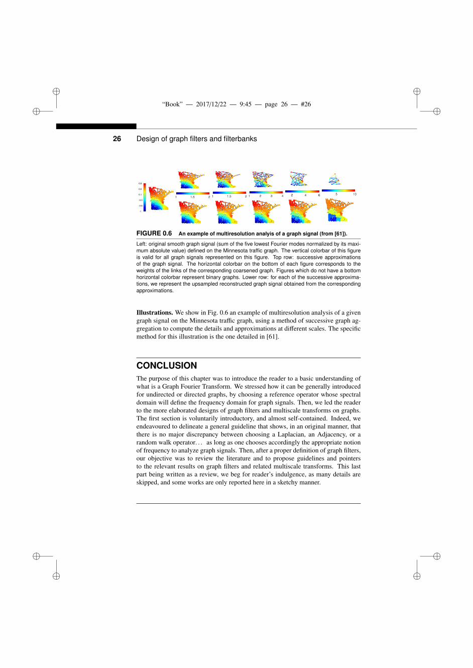
FIGURE 0.6 An example of multiresolution analyis of a graph signal (from [61]).

Left: original smooth graph signal (sum of the five lowest Fourier modes normalized by its maxi-mum absolute value) defined on the Minnesota traffic graph. The vertical colorbar of this figureis valid for all graph signals represented on this figure. Top row: successive approximationsof the graph signal. The horizontal colorbar on the bottom of each figure corresponds to theweights of the links of the corresponding coarsened graph. Figures which do not have a bottomhorizontal colorbar represent binary graphs. Lower row: for each of the successive approxima-tions, we represent the upsampled reconstructed graph signal obtained from the correspondingapproximations.

Illustrations. We show in Fig. 0.6 an example of multiresolution analysis of a givengraph signal on the Minnesota traffic graph, using a method of successive graph ag-gregation to compute the details and approximations at different scales. The specificmethod for this illustration is the one detailed in [61].

CONCLUSIONThe purpose of this chapter was to introduce the reader to a basic understanding ofwhat is a Graph Fourier Transform. We stressed how it can be generally introducedfor undirected or directed graphs, by choosing a reference operator whose spectraldomain will define the frequency domain for graph signals. Then, we led the readerto the more elaborated designs of graph filters and multiscale transforms on graphs.The first section is voluntarily introductory, and almost self-contained. Indeed, weendeavoured to delineate a general guideline that shows, in an original manner, thatthere is no major discrepancy between choosing a Laplacian, an Adjacency, or arandom walk operator. . . as long as one chooses accordingly the appropriate notionof frequency to analyze graph signals. Then, after a proper definition of graph filters,our objective was to review the literature and to propose guidelines and pointersto the relevant results on graph filters and related multiscale transforms. This lastpart being written as a review, we beg for reader’s indulgence, as many details areskipped, and some works are only reported here in a sketchy manner.

ii

“Book” — 2017/12/22 — 9:45 — page 27 — #27 ii

ii

ii


ACKNOWLEDGEMENTSWork supported by the ANR grant Graphsip ANR-14-CE27-0001-02 and ANR-14-CE27-0001-03,as well as the LabEx PERSYVAL-Lab (ANR-11-LABX-0025-01) funded by the French programInvestissement d?avenir.

ii

“Book” — 2017/12/22 — 9:45 — page 28 — #28 ii

ii

ii

ii

“Book” — 2017/12/22 — 9:45 — page 29 — #29 ii

ii

ii

[1] A. Sandryhaila and J. Moura, “Discrete signal processing on graphs,” Signal Processing, IEEETransactions on, vol. 61, no. 7, pp. 1644–1656, April 2013.

[2] D. Shuman, S. Narang, P. Frossard, A. Ortega, and P. Vandergheynst, “The emerging field ofsignal processing on graphs: Extending high-dimensional data analysis to networks and otherirregular domains,” Signal Processing Magazine, IEEE, vol. 30, no. 3, pp. 83–98, May 2013.

[3] D. Hammond, P. Vandergheynst, and R. Gribonval, “Wavelets on graphs via spectral graphtheory,” Applied and Computational Harmonic Analysis, vol. 30, no. 2, pp. 129–150, 2011.

[4] S. Narang and A. Ortega, “Perfect reconstruction two-channel wavelet filter banks for graphstructured data,” Signal Processing, IEEE Transactions on, vol. 60, no. 6, pp. 2786–2799, June2012.

[5] F. Chung, Spectral graph theory. Amer Mathematical Society, 1997, no. 92.[6] L. Grady and J. R. Polimeni, Discrete Calculus: Applied Analysis on Graphs for Computa-

tional Science. Springer, 2010.[7] A. Barrat, M. Barthlemy, and A. Vespignani, Dynamical processes on complex networks.

Cambridge University Press, 2008.[8] S. Kar and J. M. F. Moura, “Consensus + innovations distributed inference over networks:

cooperation and sensing in networked systems,” IEEE Signal Processing Magazine, vol. 30,no. 3, pp. 99–109, May 2013.

[9] H. Rabiei, F. Richard, O. Coulon, and J. Lefevre, “Local spectral analysis of the cerebralcortex: New gyrification indices,” IEEE Transactions on Medical Imaging, vol. 36, no. 3, pp.838–848, March 2017.

[10] R. Singh, A. Chakraborty, and B. S. Manoj, “Graph fourier transform based on directed lapla-cian,” in 2016 International Conference on Signal Processing and Communications (SPCOM),June 2016, pp. 1–5.

[11] H. Sevi, G. Rilling, and P. Borgnat, “Multiresolution analysis of functions on directed net-works,” in Wavelets and Sparsity XVII, Aug 2017.

[12] F. Chung, “Laplacians and the Cheeger inequality for directed graphs,” Annals ofCombinatorics, vol. 9, no. 1, pp. 1–19, 2005. [Online]. Available: http://link.springer.com/

article/10.1007/s00026-005-0237-z[13] G. Yu and H. Qu, “Hermitian laplacian matrix and positive of mixed graphs,” Applied

Mathematics and Computation, vol. 269, no. Supplement C, pp. 70 – 76, 2015. [Online].Available: http://www.sciencedirect.com/science/article/pii/S0096300315009649

[14] S. Sardellitti, S. Barbarossa, and P. D. Lorenzo, “On the graph fourier transform for directedgraphs,” IEEE Journal of Selected Topics in Signal Processing, vol. 11, no. 6, pp. 796–811,Sept 2017.

[15] R. Shafipour, A. Khodabakhsh, G. Mateos, , and E. Nikolova, “A digraph fourier transformwith spread frequency components,” in Proc. of IEEE Global Conf. on Signal and InformationProcessing, Nov 2017.

[16] A. Sandryhaila and J. Moura, “Discrete signal processing on graphs: Frequency analysis,”Signal Processing, IEEE Transactions on, vol. 62, no. 12, pp. 3042–3054, June 2014.

[17] H. Sevi, G. Rilling, and P. Borgnat, “Analyse frequentielle et filtrage sur graphes diriges,” in26e Colloque sur le Traitement du Signal et des Images. GRETSI-2017, Sept 2017, p. id. 220.

[18] S. Ben Alaya, P. Goncalves, and P. Borgnat, “Linear prediction on graphs based on autoregres-sive models,” in Graph Signal Processing Workshop, May 2016.

[19] B. Girault, P. Goncalves, and E. Fleury, “Translation on graphs : An isometric shift operator,”Signal Processing Letters, IEEE, vol. 22, no. 12, Dec. 2015.

[20] A. Anis, A. Gadde, and A. Ortega, “Efficient sampling set selection for bandlimited graph

29

ii

“Book” — 2017/12/22 — 9:45 — page 30 — #30 ii

ii

ii


signals using graph spectral proxies,” IEEE Transactions on Signal Processing, vol. 64, no. 14,pp. 3775–3789, July 2016.

[21] W. Zachary, “An information flow model for conflict and fission in small groups,” Journal ofanthropological research, vol. 33, no. 4, pp. 452–473, 1977.

[22] L. LeMagoarou, R. Gribonval, and N. Tremblay, “Approximate fast graph Fourier transformsvia multi-layer sparse approximations,” IEEE Transactions on Signal and Information Pro-cessing over Networks, vol. PP, no. 99, pp. 1–1, 2017.

[23] L. LeMagoarou, N. Tremblay, and R. Gribonval, “Analyzing the approximation error of thefast graph fourier transform,” in proceedings of the Asilomar Conference on Signals, Systems,and Computers, Nov 2017.

[24] E. Isufi, A. Loukas, A. Simonetto, and G. Leus, “Autoregressive Moving Average Graph Fil-tering,” IEEE Transactions on Signal Processing, vol. 65, no. 2, pp. 274–288, Jan. 2017.

[25] A. Loukas, A. Simonetto, and G. Leus, “Distributed autoregressive moving average graphfilters,” IEEE Signal Processing Letters, vol. 22, no. 11, pp. 1931–1935, Nov 2015.

[26] X. Shi, H. Feng, M. Zhai, T. Yang, and B. Hu, “Infinite Impulse Response Graph Filters inWireless Sensor Networks,” Signal Processing Letters, IEEE, vol. 22, no. 8, pp. 1113–1117,2015.

[27] J. Liu, E. Isufi, and G. Leus, “Autoregressive moving average graph filter design,” in 6th JointWIC/IEEE Symposium on Information Theory and Signal Processing in the Benelux, May2016.

[28] N. Perraudin and P. Vandergheynst, “Stationary signal processing on graphs,” IEEE Transac-tions on Signal Processing, vol. 65, no. 13, pp. 3462–3477, July 2017.

[29] A. G. Marques, S. Segarra, G. Leus, and A. Ribeiro, “Stationary graph processes and spectralestimation,” IEEE Transactions on Signal Processing, vol. 65, no. 22, pp. 5911–5926, Nov2017.

[30] D. Shuman, P. Vandergheynst, and P. Frossard, “Chebyshev polynomial approximation fordistributed signal processing,” in Distributed Computing in Sensor Systems and Workshops(DCOSS), 2011 International Conference on, June 2011, pp. 1–8.

[31] N. Tremblay, G. Puy, R. Gribonval, and P. Vandergheynst, “Compressive spectralclustering,” in Proceedings of the 33 rd International Conference on Machine Learning(ICML), vol. 48. JMLR: W&CP, 2016, pp. 1002–1011. [Online]. Available: http://jmlr.csail.mit.edu/proceedings/papers/v48/tremblay16.pdf

[32] A. Susnjara, N. Perraudin, D. Kressner, and P. Vandergheynst, “Accelerated filtering ongraphs using Lanczos method,” arXiv preprint arXiv:1509.04537, 2015. [Online]. Available:https://arxiv.org/abs/1509.04537

[33] E. Gallopoulos and Y. Saad, “Efficient Solution of Parabolic Equations by KrylovApproximation Methods,” SIAM Journal on Scientific and Statistical Computing, vol. 13,no. 5, pp. 1236–1264, 1992. [Online]. Available: https://doi.org/10.1137/0913071

[34] Y. Saad, Numerical Methods for Large Eigenvalue Problems, 2nd ed., ser. Classics in AppliedMathematics 66. SIAM, 2011.

[35] M. Crovella and E. Kolaczyk, “Graph wavelets for spatial traffic analysis,” in INFOCOM 2003.Twenty-Second Annual Joint Conference of the IEEE Computer and Communications. IEEESocieties, vol. 3, 2003, pp. 1848–1857.

[36] R. Coifman and M. Maggioni, “Diffusion wavelets,” Applied and Computational HarmonicAnalysis, vol. 21, no. 1, pp. 53–94, 2006.

[37] M. Gavish, B. Nadler, and R. R. Coifman, “Multiscale wavelets on trees, graphs and highdimensional data: Theory and applications to semi supervised learning,” in Proceedings of the

ii

“Book” — 2017/12/22 — 9:45 — page 31 — #31 ii

ii

ii


27th International Conference on Machine Learning (ICML-10), 2010, pp. 367–374.[38] G. Strang and T. Nguyen, Wavelets and filter banks. SIAM, 1996.[39] M. Maggioni and H. Mhaskar, “Diffusion polynomial frames on metric measure spaces,”

Applied and Computational Harmonic Analysis, vol. 24, no. 3, pp. 329–353, May 2008.[Online]. Available: http://linkinghub.elsevier.com/retrieve/pii/S106352030700070X

[40] N. Leonardi and D. Van De Ville, “Tight wavelet frames on multislice graphs,” Signal Process-ing, IEEE Transactions on, vol. 61, no. 13, pp. 3357–3367, July 2013.

[41] D. Shuman, C. Wiesmeyr, N. Holighaus, and P. Vandergheynst, “Spectrum-adapted tight graphwavelet and vertex-frequency frames,” Signal Processing, IEEE Transactions on, vol. PP,no. 99, pp. 1–1, 2015.

[42] O. Teke and P. P. Vaidyanathan, “Extending Classical Multirate Signal Processing Theory toGraphs ; Part I: Fundamentals,” IEEE Transactions on Signal Processing, vol. 65, no. 2, pp.409–422, Jan. 2017.

[43] V. N. Ekambaram, G. C. Fanti, B. Ayazifar, and K. Ramchandran, “Circulant structures andgraph signal processing,” in 2013 IEEE International Conference on Image Processing, Sep.2013, pp. 834–838.

[44] M. S. Kotzagiannidis and P. L. Dragotti, “Splines and wavelets on circulant graphs,” CoRR,vol. abs/1603.04917, 2016. [Online]. Available: http://arxiv.org/abs/1603.04917

[45] D. I. Shuman, M. J. Faraji, and P. Vandergheynst, “A Multiscale Pyramid Transform for GraphSignals,” IEEE Transactions on Signal Processing, vol. 64, no. 8, pp. 2119–2134, Apr. 2016.

[46] A. Sakiyama and Y. Tanaka, “Oversampled graph Laplacian matrix for graph filter banks,”Signal Processing, IEEE Transactions on, vol. 62, no. 24, pp. 6425–6437, Dec 2014.

[47] H. Nguyen and M. Do, “Downsampling of signals on graphs via maximum spanning trees,”Signal Processing, IEEE Transactions on, vol. 63, no. 1, pp. 182–191, Jan 2015.

[48] S. Narang and A. Ortega, “Local two-channel critically sampled filter-banks on graphs,” inImage Processing (ICIP), 2010 17th IEEE International Conference on, Sept 2010, pp. 333–336.

[49] L. Avena, F. Castell, A. Gaudilliere, and C. Melot, “Intertwining wavelets or Multiresolutionanalysis on graphs through random forests,” 2017.

[50] S. Lafon and A. B. Lee, “Diffusion maps and coarse-graining: a unified framework for dimen-sionality reduction, graph partitioning, and data set parameterization,” IEEE Transactions onPattern Analysis and Machine Intelligence, vol. 28, no. 9, pp. 1393–1403, Sep. 2006.

[51] O. E. Livne and A. Brandt, “Lean Algebraic Multigrid (LAMG): Fast Graph LaplacianLinear Solver,” SIAM Journal on Scientific Computing, vol. 34, no. 4, pp. B499–B522, 2012.[Online]. Available: https://doi.org/10.1137/110843563

[52] D. Ron, I. Safro, and A. Brandt, “Relaxation-based coarsening and multiscale graphorganization,” Multiscale Modeling & Simulation, vol. 9, no. 1, pp. 407–423, 2011. [Online].Available: http://epubs.siam.org/doi/abs/10.1137/100791142

[53] I. Dhillon, Y. Guan, and B. Kulis, “Weighted Graph Cuts without Eigenvectors A MultilevelApproach,” Pattern Analysis and Machine Intelligence, IEEE Transactions on, vol. 29, no. 11,pp. 1944–1957, Nov. 2007.

[54] G. Karypis and V. Kumar, “A Fast and High Quality Multilevel Scheme for PartitioningIrregular Graphs,” SIAM Journal on Scientific Computing, vol. 20, no. 1, pp. 359–392, 1998.[Online]. Available: http://dx.doi.org/10.1137/S1064827595287997

[55] F. Murtagh and P. Contreras, “Algorithms for hierarchical clustering: an overview,” WileyInterdisciplinary Reviews: Data Mining and Knowledge Discovery, vol. 2, no. 1, pp. 86–97,2012. [Online]. Available: http://dx.doi.org/10.1002/widm.53

ii

“Book” — 2017/12/22 — 9:45 — page 32 — #32 ii

ii

ii


[56] M. E. Newman, “Modularity and community structure in networks,” Proceedings of the Na-tional Academy of Sciences, vol. 103, no. 23, pp. 8577–8582, 2006.

[57] S. Fortunato, “Community detection in graphs,” Physics Reports, vol. 486, no. 3-5, pp. 75–174,2010.

[58] J. Reichardt and S. Bornholdt, “Statistical mechanics of community detection,” Phys. Rev.E, vol. 74, no. 1, p. 016110, Jul. 2006. [Online]. Available: http://link.aps.org/doi/10.1103/

PhysRevE.74.016110[59] M. Schaub, J. Delvenne, S. Yaliraki, and M. Barahona, “Markov dynamics as a zooming lens

for multiscale community detection: non clique-like communities and the field-of-view limit,”PloS one, vol. 7, no. 2, p. e32210, 2012.

[60] N. Tremblay and P. Borgnat, “Graph Wavelets for Multiscale Community Mining,” SignalProcessing, IEEE Transactions on, vol. 62, no. 20, pp. 5227–5239, Oct. 2014.

[61] ——, “Subgraph-Based Filterbanks for Graph Signals,” IEEE Transactions on Signal Process-ing, vol. 64, no. 15, pp. 3827–3840, Aug. 2016.

[62] J. Irion and N. Saito, “Applied and computational harmonic analysis on graphs and networks,”in Wavelets and Sparsity XVI, vol. 9597, Sep. 2015, pp. 95 971F–95 971F–15. [Online].Available: http://dx.doi.org/10.1117/12.2186921

[63] A. B. Lee, B. Nadler, and L. Wasserman, “Treelets: An Adaptive Multi-Scale Basis for SparseUnordered Data,” The Annals of Applied Statistics, vol. 2, no. 2, pp. 435–471, 2008. [Online].Available: http://www.jstor.org/stable/30244207

[64] G. Mishne, R. Talmon, I. Cohen, R. R. Coifman, and Y. Kluger, “Data-Driven Tree Transformsand Metrics,” IEEE Transactions on Signal and Information Processing over Networks, vol. PP,no. 99, pp. 1–1, 2017.

[65] A. D. Szlam, M. Maggioni, R. R. Coifman, and J. C. Bremer Jr, “Diffusion-driven multiscaleanalysis on manifolds and graphs: top-down and bottom-up constructions,” in Proc SPIE, vol.5914, 2005, p. 59141D.

[66] D. A. Spielman and N. Srivastava, “Graph Sparsification by Effective Resistances,”SIAM Journal on Computing, vol. 40, no. 6, pp. 1913–1926, 2011. [Online]. Available:http://dx.doi.org/10.1137/080734029

Documents

Design of graph filters and filterbanks