Embed Size (px)
Citation preview
Graduate Theses, Dissertations, and Problem Reports
2019
Design of Geothermal District Heating and Cooling System for the Design of Geothermal District Heating and Cooling System for the
West Virginia University West Virginia University
OLUWASOGO BOLAJI ALONGE West Virginia University, [email protected]
Follow this and additional works at: https://researchrepository.wvu.edu/etd
Part of the Other Chemical Engineering Commons
Recommended Citation Recommended Citation ALONGE, OLUWASOGO BOLAJI, "Design of Geothermal District Heating and Cooling System for the West Virginia University" (2019). Graduate Theses, Dissertations, and Problem Reports. 7397. https://researchrepository.wvu.edu/etd/7397
This Thesis is protected by copyright and/or related rights. It has been brought to you by the The Research Repository @ WVU with permission from the rights-holder(s). You are free to use this Thesis in any way that is permitted by the copyright and related rights legislation that applies to your use. For other uses you must obtain permission from the rights-holder(s) directly, unless additional rights are indicated by a Creative Commons license in the record and/ or on the work itself. This Thesis has been accepted for inclusion in WVU Graduate Theses, Dissertations, and Problem Reports collection by an authorized administrator of The Research Repository @ WVU. For more information, please contact [email protected].
Design of Geothermal District Heating and Cooling
System for the West Virginia University
Oluwasogo Bolaji Alonge
Thesis submitted
to the Benjamin M. Statler College of Engineering and Mineral Resources
at West Virginia University
in partial fulfillment of the requirements for the degree of
Master of Science in
Chemical Engineering
Nagasree Garapati, Ph.D., P.E., Chair
Fernando Lima, Ph.D.
Debangsu Bhattacharyya, Ph.D.
Department of Chemical Engineering
Morgantown, West Virginia
2019
Keywords: Levelized cost of heat, Geothermal, District heating and cooling
system, Steam-based system, GEOPHIRES, Aspen simulators, HYSYS,
Surface plant, West Virginia University.
Copyright 2019 Oluwasogo Bolaji Alonge

Abstract
Design of Geothermal District Heating and Cooling System for the West Virginia
University
Oluwasogo Bolaji Alonge
Recent Appalachian Basin Geothermal Play Fairway Analysis estimated elevated heat flows in
north-central West Virginia. This region provides an optimal and unique combination of elevated
temperatures and flow necessary for geothermal development along with year-round surface
demand for heating and cooling on the campus. Therefore, West Virginia University’s (WVU’s)
Morgantown campus has been identified as a prime location in the eastern United States for the
development of a geothermal direct-use heating and cooling application.
The objective of this study was to perform a feasibility analysis for the development of a
geothermal district heating and cooling (GDHC) system for WVU campus in Morgantown, WV,
to replace the current coal-fired steam heating and cooling system. A hybrid GDHC system is
proposed to replace the existing system based on the data collected the project period from the
existing district heating and cooling (DHC) facilities and Aspen simulations were conducted to
analyze two scenarios for the design of a heating and cooling system at WVU’s Morgantown
campus and calculate surface plant capital costs. Scenario 1 would supply superheated steam to
the entire campus and Scenario 2 would deliver saturated steam to the Health Sciences and
Evansdale campuses. The overall economics of the geothermal system was performed using
modified GEOPHIRES. For the two scenarios considered, geothermal contribution to the heating
and cooling on WVU campus is around 2.30 to 2.43% and 4.05 to 4.39% for hybrid geothermal
system and improved hybrid geothermal system with heat pump, respectively.
Currently, WVU pays $15/MMBTU for steam supplied by the Morgantown Energy Associates
(MEA) coal-fired power plant. Utilizing the existing pipeline distribution system, this study results
yielded the levelized cost of heat (LCOH) for the two scenario designs in the ranges of 7.55 to
10.90 $/MMBTU for vertical well configuration and 7.77 to 11.60 $/MMBTU for horizontal well
configuration which is well below the current price for steam supplied by MEA. To address
uncertainty related to the distribution systems, LCOH was calculated in GEOPHIRES for a case
where existing pipelines are to be purchased from MEA and for an instance where a new set of
pipelines are to be installed by WVU. Purchasing or installing new pipeline distribution facilities
if existing pipeline networks are not donated by MEA resulted in LCOH in the range of 8.50 to
14.08 $/MMBTU which shows that LCOH values increase with additional capital cost for the
distribution pipelines. However, the range of LCOH values calculated for the natural gas fired
boiler (NGFB) system without geothermal (5.65 to 7.46 $/MMBTU) is comparably lower than the
range of values obtained for the proposed hybrid GDHC system. Nevertheless, the proposed hybrid
GDHC system for WVU can provide clean energy to replace the existing MEA coal-fired, steam-
based system; hence, providing an alternative to offset the impacts from fossil fuels consumption.
Further, analysis of the future price of fuel showed that proposed hybrid system will be more
economical compared to NGFB at a natural price of about $15.00/1000ft3.

iii
Dedicated to the Glory of Almighty God
“the Holy One of Israel”

iv
Acknowledgements
I would like to offer a thankful note to several individuals and organizations that have supported
me in the course of my thesis.
First and foremost, I would like to express my deepest appreciation to my advisor, Dr. Nagasree
Garapati, who has provided many ingenious suggestions from the start of the project to the end.
Without her numerous suggestions and remarkable contributions, the goal of this project would
not have been realized. I have greatly benefitted from her guidance and illustrious suggestions and
I considered it a great privilege for providing me the opportunity to work on the project.
I would like to thank my committee members, Dr. Lima and Dr. Bhattacharyya for their inputs and
insightful recommendations in the course of this project. I am extremely grateful for their help,
feedback and guidance at different phases of the project. This thesis completion would not have
been possible without the support and nurturing from my committee from time to time.
I would also like to extend my gratitude to Dr. Richard Turton for creating time out of his busy
schedule to review the thesis document and for ensuring the successful completion of this project.
I am deeply indebted to your valuable advice in the course of writing this thesis.
I am grateful to Dr. Koenraad Beckers for the help and suggestions in editing the GEOPHIRES
codes for a hybrid system. I would also like to express my gratitude to U.S. Department of Energy
for providing the platform to work on this project through the project funding. I would also like to
appreciate the WVU Facilities Management for providing to some of the data and drawings, and
for the warmth reception at various meetings. I am also thankful to the following colleagues:
Selorme Agbleze, Brent Bishop, Shuyun Li, Paul Akula and Dr. Oluwaotosin Oginni for the
wonderful moments we have shared together.
Finally, I would like to acknowledge the support of my parents and family for providing me with
unflinching support and unrelenting inspiration throughout the duration of this thesis. This
accomplishment would not have been possible without their encouragement.
v
Table of Contents
Abstract ...................................................................................................................................... iii
Table of Contents ........................................................................................................................ v
List of Tables .............................................................................................................................. ix
List of Figures .......................................................................................................................... xiii
Introduction ........................................................................................................................................... 1
1.1 Background ...................................................................................................................... 1
1.2 Geothermal Energy as a Renewable Energy Source ........................................................ 3
1.3 Objectives and Approach ................................................................................................. 6
1.4 Thesis Structure ................................................................................................................ 7
Literature Review .................................................................................................................................. 8
2.1 Development of Geothermal District Heating and cooling (GDHC) System in US. ....... 8
2.2 Surface Plant Development .............................................................................................. 9
2.3 Overview of district heating and cooling (DHC) system at WVU ................................ 10
2.3.1 Existing Heating and Cooling System at WVU .................................................................. 10
2.3.2 Proposed Heating and Cooling System at WVU ................................................................ 10
2.3.3 The Research Study Workflow ........................................................................................... 10
Characterization of Existing Infrastructure and Evaluation of Existing Campus District Heating (DH)
System Retrofit Capability .......................................................................................................................... 12
3.1 Objective 1: Characterization of Existing Infrastructure ............................................... 12
3.2 Objective 1: Results and Discussion .............................................................................. 12
3.3 Objective 2: Evaluate Existing Campus District Heating (DH) System Retrofit
Capability .................................................................................................................................. 14
3.4 Objective 2: Results and Discussion .............................................................................. 14
Objective 3: Design a Surface Plant and Pipeline Distribution Using Aspen Simulators .................. 15
4.1 Proposed Hybrid Geothermal-Natural Gas System Design ........................................... 15
4.2 Geothermal Heat Exchanger Unit .................................................................................. 19
vi
4.3 Fired heater simulation in HYSYS................................................................................. 20
4.4 Distribution Piping System ............................................................................................ 24
4.4.1 The major assumptions and conditions used in distribution pipeline simulation for the
entire campus include: ........................................................................................................................ 24
4.4.2 Pipeline Elevation ............................................................................................................... 25
4.4.3 Steam distribution pipelines ................................................................................................ 26
4.4.4 Condensate return pipelines ................................................................................................ 27
4.5 Heat Pump System ......................................................................................................... 29
4.5.1 Heat Pump Principle ........................................................................................................... 29
4.5.2 Selection of working fluid ................................................................................................... 30
Objective 3: Results and Discussion ................................................................................................... 32
5.1 Geothermal Heat Exchanger Unit Results and Discussion ............................................ 32
5.1.1 Scenario 1 Heat Exchanger: ................................................................................................ 33
5.1.2 Scenario 2 Heat Exchanger: ................................................................................................ 34
5.2 Geothermal Contribution to the Heating and Cooling System at WVU Results and
Discussion ................................................................................................................................. 35
5.2.1 Scenario 1 Geothermal Contribution .................................................................................. 35
5.2.2 Scenario 2 Geothermal Contribution .................................................................................. 39
5.3 Boiler Unit: Fired Heater Results and Discussion ......................................................... 42
5.3.1 Fired Heater Inlet Conditions: ............................................................................................. 42
5.4 Ammonia (NH3) Heat Pump System ............................................................................. 46
5.5 Vendors Quote for Heat Pump and Boiler ..................................................................... 49
5.5.1 Boiler Vendor’s Quote from Johnston Boiler Company (JBC): ......................................... 49
5.5.2 Heat Pump Vendor’s Quote from Mayekawa Company: ................................................... 50
5.6 HYSYS Pipeline Distribution System Simulations Results and Discussion ................. 51
5.6.1 Pressure losses across steam line: ....................................................................................... 51
5.6.2 Pressure losses across condensate line: ............................................................................... 53
vii
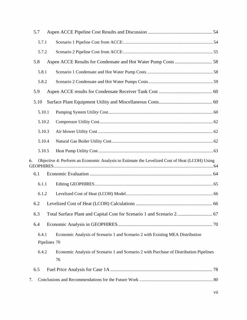
5.7 Aspen ACCE Pipeline Cost Results and Discussion ..................................................... 54
5.7.1 Scenario 1 Pipeline Cost from ACCE: ................................................................................ 54
5.7.2 Scenario 2 Pipeline Cost from ACCE: ................................................................................ 55
5.8 Aspen ACCE Results for Condensate and Hot Water Pump Costs ............................... 58
5.8.1 Scenario 1 Condensate and Hot Water Pump Costs ........................................................... 58
5.8.2 Scenario 2 Condensate and Hot Water Pumps Costs .......................................................... 59
5.9 Aspen ACCE results for Condensate Receiver Tank Cost ............................................ 60
5.10 Surface Plant Equipment Utility and Miscellaneous Costs ............................................ 60
5.10.1 Pumping System Utility Cost .............................................................................................. 60
5.10.2 Compressor Utility Cost ...................................................................................................... 62
5.10.3 Air blower Utility Cost ....................................................................................................... 62
5.10.4 Natural Gas Boiler Utility Cost ........................................................................................... 62
5.10.5 Heat Pump Utility Cost ....................................................................................................... 63
Objective 4: Perform an Economic Analysis to Estimate the Levelized Cost of Heat (LCOH) Using
GEOPHIRES............................................................................................................................................... 64
6.1 Economic Evaluation ..................................................................................................... 64
6.1.1 Editing GEOPHIRES .......................................................................................................... 65
6.1.2 Levelized Cost of Heat (LCOH) Model .............................................................................. 66
6.2 Levelized Cost of Heat (LCOH) Calculations ............................................................... 66
6.3 Total Surface Plant and Capital Cost for Scenario 1 and Scenario 2. ............................ 67
6.4 Economic Analysis in GEOPHIRES.............................................................................. 70
6.4.1 Economic Analysis of Scenario 1 and Scenario 2 with Existing MEA Distribution
Pipelines 70
6.4.2 Economic Analysis of Scenario 1 and Scenario 2 with Purchase of Distribution Pipelines
76
6.5 Fuel Price Analysis for Case 1A .................................................................................... 78
Conclusions and Recommendations for the Future Work .................................................................. 80

viii
7.1 Conclusions .................................................................................................................... 80
7.2 Recommendations for the Future Work ......................................................................... 83

ix
List of Tables
Table 4.1: Air and fuel inlet conditions for fired heater simulation in HYSYS. .......................... 23
Table 4.2: The elevation changes used in pipeline simulations in HYSYS. ................................. 25
Table 5.1: The results of HYSYS simulation of geothermal plate heat exchanger (PHE). .......... 32
Table 5.2: Results of rigorous design of plate heat exchanger (PHE) in EDR for Scenario 1.
........................................................................................................ Error! Bookmark not defined.
Table 5.3: Results of rigorous design of plate heat exchanger (PHE) in EDR for Scenario 2. .... 34
Table 5.4: Results for Case 1A simulated in HYSYS for geothermal contribution to a hybrid
geothermal system without heat pump (%GEO) to produce superheated steam at 18.25 bar and
260°C using geothermal fluid flow rate of 15.2 kg/s and varying monthly steam flow rate. ....... 36
Table 5.5: Results for Case 1A simulated in HYSYS for geothermal contribution to the improved
hybrid geothermal system using heat pump (%GEOHP) to produce superheated steam at 18.25 bar
and 260°C using geothermal fluid flow rate of 15.2 kg/s and varying monthly steam flow rate. 37
Table 5.6: Results for Case 1B simulated in HYSYS for geothermal contribution to a hybrid
geothermal system without heat pump (%GEO) to produce superheated steam at 14.25 bar and
200°C for Med-Center, Towers, Evansdale, and Downtown meter points, and the compressor
producing superheated steam at 18.25 bar and 260°C for Life Sciences meter point using
geothermal fluid flow rate of 15.2 kg/s. ........................................................................................ 38
Table 5.7: Results for Case 1B simulated in HYSYS for geothermal contribution to the improved
hybrid geothermal system using heat pump (%GEOHP) to produce superheated steam at 14.25 bar
and 200°C for Med-Center, Towers, Evansdale, and Downtown meter points, and the compressor
producing superheated steam at 18.25 bar and 260°C for Life Sciences meter point using
geothermal fluid flow rate of 15.2 kg/s. ........................................................................................ 38
Table 5.8: Results for Case 2A simulated in HYSYS for geothermal contribution to a hybrid
geothermal system without heat pump (%GEO) to produce superheated steam at 12.5 bar using
geothermal fluid flow rate of 10.2 kg/s. ........................................................................................ 39
Table 5.9: Results for Case 2A simulated in HYSYS for geothermal contribution to the improved
hybrid geothermal system using heat pump (%GEOHP) to produce superheated steam at 12.5 bar
using geothermal fluid flow rate of 10.2 kg/s. .............................................................................. 40
Table 5.10: Results for Case 2B for geothermal contribution to a hybrid geothermal system without
heat pump (%GEO) with two boilers: one producing saturated steam at 12.5 bar for Evansdale and

x
Medical Center meter points, and the second boiler producing low pressure steam at 2.75 bar for
Towers using geothermal fluid flow rate of 10.2 kg/s. ................................................................. 41
Table 5.11: Results for Case 2B for geothermal contribution to the improved hybrid geothermal
system using heat pump (%GEOHP) with two boilers: one producing saturated steam at 12.5 bar
for Evansdale and Med-Center meter points, and the second boiler producing low pressure steam
at 2.75 bar for Towers using geothermal fluid flow rate of 10.2 kg/s. ......................................... 41
Table 5.12: The data obtained from HYSYS simulation of natural gas fuel preheater for Scenario
1..................................................................................................................................................... 42
Table 5.13: The data obtained from HYSYS simulation of natural gas fuel preheater for Scenario
2..................................................................................................................................................... 43
Table 5.15: Inlet hot water, flue gas and high pressure steam outlet conditions for the combustion
of natural gas simulated in HYSYS fired heater for Case 1A and Case 1B obtained at a fixed boiler
efficiency of η=85%, a fixed boiler hot water inlet temperature of 90°C for a given natural gas
flow rate. ....................................................................................................................................... 43
Table 5.17: Inlet hot water, flue gas and high pressure steam outlet conditions for the combustion
of natural gas simulated in HYSYS fired heater for Case 2A and Case 2B obtained at a fixed boiler
efficiency of η=85%, a fixed boiler hot water inlet temperature of 90°C for a given natural gas
flow rate. ....................................................................................................................................... 45
Table 5.19: Results of rigorous design in EDR and Aspen ACCE estimation for the natural gas
preheater (shell and tube heat exchanger) for Scenario 1 and Scenario 2. ................................... 46
Table 5.20: Results of the coefficient of performance for Scenario 1 and Scenario 2. ................ 48
Table 5.21: Vendor’s quote obtained from Johnston Boiler Company (JBC) for Scenario 1 and
Scenario 2 boilers simulated in HYSYS. ...................................................................................... 49
Table 5.23: High temperature heat pump package performance obtained from Mayekawa
Company. ...................................................................................................................................... 50
Table 5.24: Mayekawa Company ammonia heat pump quote parameters compared to Aspen
Scenario 1 and Scenario 2 heat pump parameters simulated in HYSYS. Red section represents the
heat pump system conditions obtained from HYSYS simulation. ............................................... 51
Table 5.25: Pressure drop across the steam pipelines for Scenario 2 (Case 1A and Case 1B). Red
section represents new pipelines and black section represents existing MEA pipelines. ............. 52
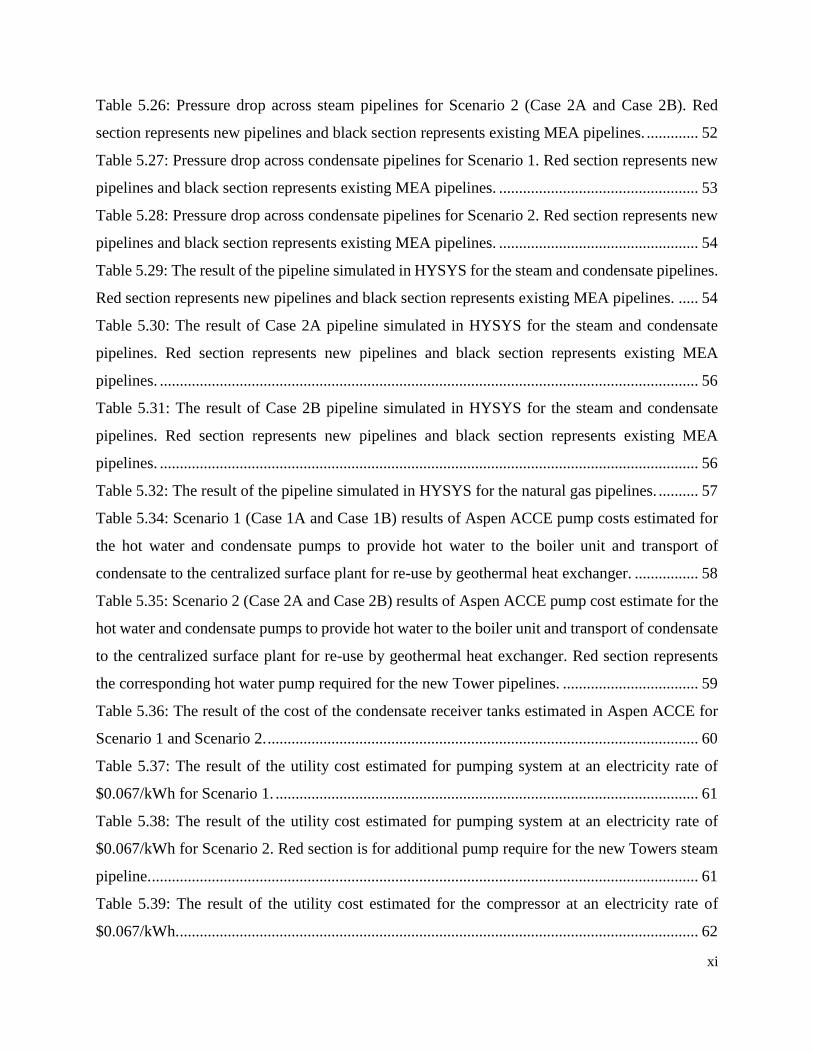
xi
Table 5.26: Pressure drop across steam pipelines for Scenario 2 (Case 2A and Case 2B). Red
section represents new pipelines and black section represents existing MEA pipelines. ............. 52
Table 5.27: Pressure drop across condensate pipelines for Scenario 1. Red section represents new
pipelines and black section represents existing MEA pipelines. .................................................. 53
Table 5.28: Pressure drop across condensate pipelines for Scenario 2. Red section represents new
pipelines and black section represents existing MEA pipelines. .................................................. 54
Table 5.29: The result of the pipeline simulated in HYSYS for the steam and condensate pipelines.
Red section represents new pipelines and black section represents existing MEA pipelines. ..... 54
Table 5.30: The result of Case 2A pipeline simulated in HYSYS for the steam and condensate
pipelines. Red section represents new pipelines and black section represents existing MEA
pipelines. ....................................................................................................................................... 56
Table 5.31: The result of Case 2B pipeline simulated in HYSYS for the steam and condensate
pipelines. Red section represents new pipelines and black section represents existing MEA
pipelines. ....................................................................................................................................... 56
Table 5.32: The result of the pipeline simulated in HYSYS for the natural gas pipelines. .......... 57
Table 5.34: Scenario 1 (Case 1A and Case 1B) results of Aspen ACCE pump costs estimated for
the hot water and condensate pumps to provide hot water to the boiler unit and transport of
condensate to the centralized surface plant for re-use by geothermal heat exchanger. ................ 58
Table 5.35: Scenario 2 (Case 2A and Case 2B) results of Aspen ACCE pump cost estimate for the
hot water and condensate pumps to provide hot water to the boiler unit and transport of condensate
to the centralized surface plant for re-use by geothermal heat exchanger. Red section represents
the corresponding hot water pump required for the new Tower pipelines. .................................. 59
Table 5.36: The result of the cost of the condensate receiver tanks estimated in Aspen ACCE for
Scenario 1 and Scenario 2. ............................................................................................................ 60
Table 5.37: The result of the utility cost estimated for pumping system at an electricity rate of
$0.067/kWh for Scenario 1. .......................................................................................................... 61
Table 5.38: The result of the utility cost estimated for pumping system at an electricity rate of
$0.067/kWh for Scenario 2. Red section is for additional pump require for the new Towers steam
pipeline. ......................................................................................................................................... 61
Table 5.39: The result of the utility cost estimated for the compressor at an electricity rate of
$0.067/kWh. .................................................................................................................................. 62

xii
Table 5.40: The result of the utility cost estimated for the air blower at an electricity rate of
$0.067/kWh. .................................................................................................................................. 62
Table 5.41: Scenario 1 and Scenario 2 results of the utility cost estimated for natural gas supply at
a rate of $4.12/1000 ft3.................................................................................................................. 63
Table 6.2: Aspen ACCE results, vendors quote and utility costs for the surface plant equipment
for Scenario 1 which supplies superheated steam to the entire campus and for Scenario 2 which
supplies saturated steam to Health Sciences and Evansdale (Towers and Evansdale) campuses. 68
Table 6.3: Natural gas boiler Aspen ACCE results, vendors quote and utility costs for the surface
plant equipment for Scenario 1 which supplies superheated steam to the entire campus and for
Scenario 2 which supplies saturated steam to Health Sciences and Evansdale (Towers and
Evansdale) campuses. ................................................................................................................... 69
Table 6.5: Parameters input into GEOPHIRES for Scenario 1 and Scenario 2 Hybrid GDHC
system at WVU. ............................................................................................................................ 70
Table 6.6: Aspen simulators output, surface technical parameters, utility costs, total capital costs
and O&M costs fed into GEOPHIRES to determine LCOH at WVU. ........................................ 73
Table 6.7: The results of economic analysis for Scenario 1 and Scenario 2 simulated in
GEOPHIRES for the vertical well. ............................................................................................... 74
Table 6.8: The results of economic analysis for Scenario 1 and Scenario 2 simulated in
GEOPHIRES for the horizontal well. ........................................................................................... 75
Table 6.9: The results of excel LCOH calculation for NGFB using BICYCLE economic model for
Scenario 1 and Scenario 2. ............................................................................................................ 78
Table 6.10: The LCOH results of the proposed hybrid GDHC system compared with NGFB system
at different natural gas prices for Case 1A.................................................................................... 79
xiii
List of Figures
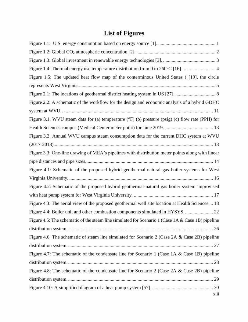
Figure 1.1: U.S. energy consumption based on energy source [1]. ............................................... 1
Figure 1.2: Global CO2 atmospheric concentration [2]. ................................................................. 2
Figure 1.3: Global investment in renewable energy technologies [3]. ........................................... 3
Figure 1.4: Thermal energy use temperature distribution from 0 to 260°C [16]. ........................... 4
Figure 1.5: The updated heat flow map of the conterminous United States ( [19], the circle
represents West Virginia. ................................................................................................................ 5
Figure 2.1: The locations of geothermal district heating system in US [27]. ................................. 8
Figure 2.2: A schematic of the workflow for the design and economic analysis of a hybrid GDHC
system at WVU. ............................................................................................................................ 11
Figure 3.1: WVU steam data for (a) temperature (°F) (b) pressure (psig) (c) flow rate (PPH) for
Health Sciences campus (Medical Center meter point) for June 2019. ........................................ 13
Figure 3.2: Annual WVU campus steam consumption data for the current DHC system at WVU
(2017-2018)................................................................................................................................... 13
Figure 3.3: One-line drawing of MEA’s pipelines with distribution meter points along with linear
pipe distances and pipe sizes......................................................................................................... 14
Figure 4.1: Schematic of the proposed hybrid geothermal-natural gas boiler systems for West
Virginia University. ...................................................................................................................... 16
Figure 4.2: Schematic of the proposed hybrid geothermal-natural gas boiler system improvised
with heat pump system for West Virginia University. ................................................................. 17
Figure 4.3: The aerial view of the proposed geothermal well site location at Health Sciences. .. 18
Figure 4.4: Boiler unit and other combustion components simulated in HYSYS. ....................... 22
Figure 4.5: The schematic of the steam line simulated for Scenario 1 (Case 1A & Case 1B) pipeline
distribution system. ....................................................................................................................... 26
Figure 4.6: The schematic of steam line simulated for Scenario 2 (Case 2A & Case 2B) pipeline
distribution system. ....................................................................................................................... 27
Figure 4.7: The schematic of the condensate line for Scenario 1 (Case 1A & Case 1B) pipeline
distribution system. ....................................................................................................................... 28
Figure 4.8: The schematic of the condensate line for Scenario 2 (Case 2A & Case 2B) pipeline
distribution system. ....................................................................................................................... 29
Figure 4.10: A simplified diagram of a heat pump system [57]. .................................................. 30
xiv
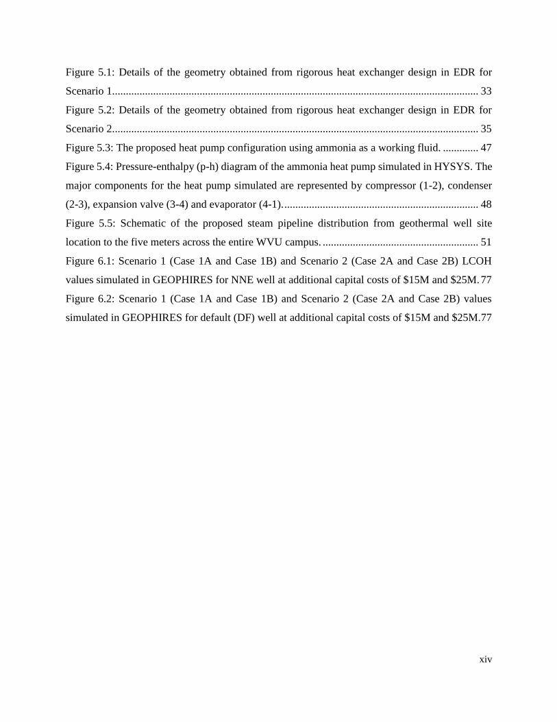
Figure 5.1: Details of the geometry obtained from rigorous heat exchanger design in EDR for
Scenario 1...................................................................................................................................... 33
Figure 5.2: Details of the geometry obtained from rigorous heat exchanger design in EDR for
Scenario 2...................................................................................................................................... 35
Figure 5.3: The proposed heat pump configuration using ammonia as a working fluid. ............. 47
Figure 5.4: Pressure-enthalpy (p-h) diagram of the ammonia heat pump simulated in HYSYS. The
major components for the heat pump simulated are represented by compressor (1-2), condenser
(2-3), expansion valve (3-4) and evaporator (4-1). ....................................................................... 48
Figure 5.5: Schematic of the proposed steam pipeline distribution from geothermal well site
location to the five meters across the entire WVU campus. ......................................................... 51
Figure 6.1: Scenario 1 (Case 1A and Case 1B) and Scenario 2 (Case 2A and Case 2B) LCOH
values simulated in GEOPHIRES for NNE well at additional capital costs of $15M and $25M. 77
Figure 6.2: Scenario 1 (Case 1A and Case 1B) and Scenario 2 (Case 2A and Case 2B) values
simulated in GEOPHIRES for default (DF) well at additional capital costs of $15M and $25M.77
1
Introduction
1.1 Background
Energy production and consumption have been around for centuries; during early civilization,
sunlight was used for making fire and wood was burned for cooking and heat. However, since the
industrial revolution, large-scale energy production became a global trend with fossil fuels
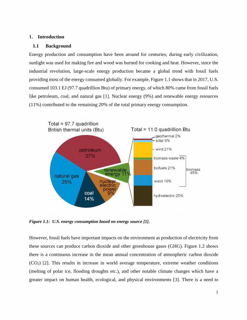
providing most of the energy consumed globally. For example, Figure 1.1 shows that in 2017, U.S.
consumed 103.1 EJ (97.7 quadrillion Btu) of primary energy, of which 80% came from fossil fuels
like petroleum, coal, and natural gas [1]. Nuclear energy (9%) and renewable energy resources
(11%) contributed to the remaining 20% of the total primary energy consumption.
Figure 1.1: U.S. energy consumption based on energy source [1].
However, fossil fuels have important impacts on the environment as production of electricity from
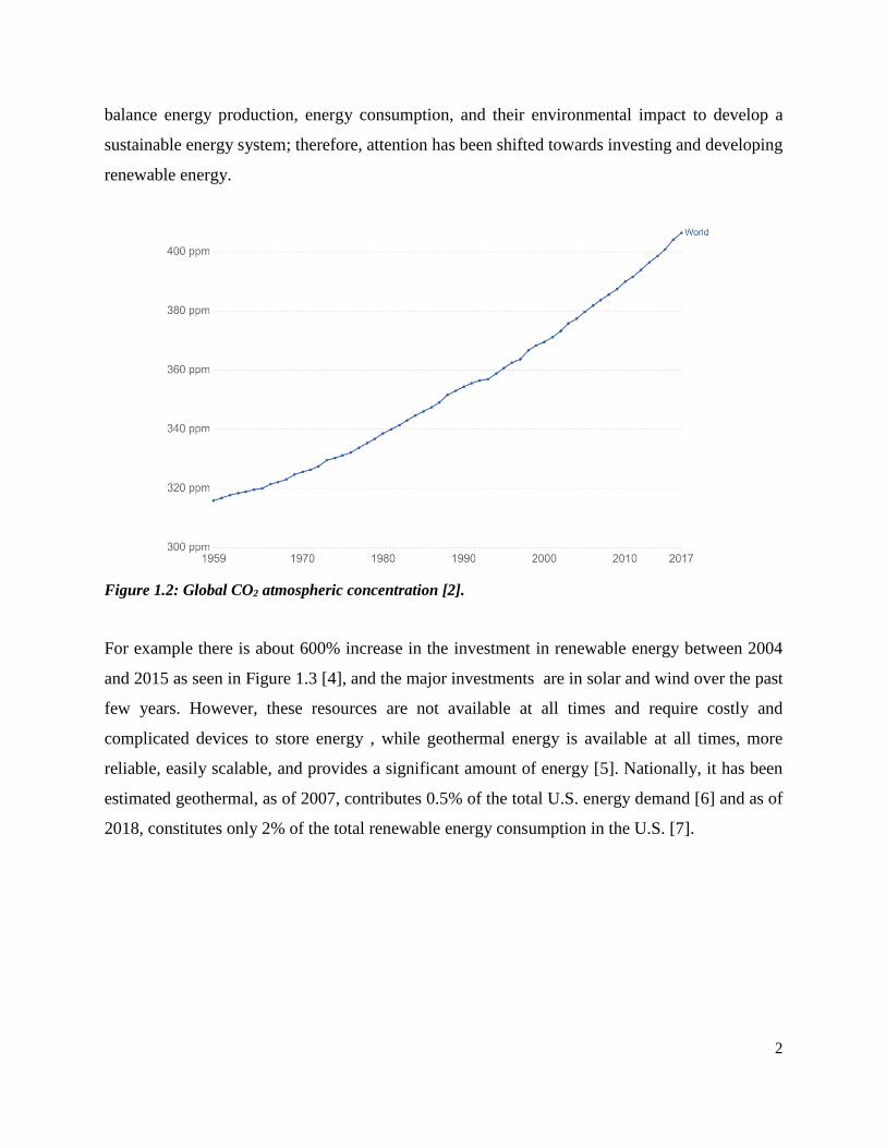
these sources can produce carbon dioxide and other greenhouse gases (GHG). Figure 1.2 shows
there is a continuous increase in the mean annual concentration of atmospheric carbon dioxide
(CO2) [2]. This results in increase in world average temperature, extreme weather conditions
(melting of polar ice, flooding droughts etc.), and other notable climate changes which have a
greater impact on human health, ecological, and physical environments [3]. There is a need to
2
balance energy production, energy consumption, and their environmental impact to develop a
sustainable energy system; therefore, attention has been shifted towards investing and developing
renewable energy.
Figure 1.2: Global CO2 atmospheric concentration [2].
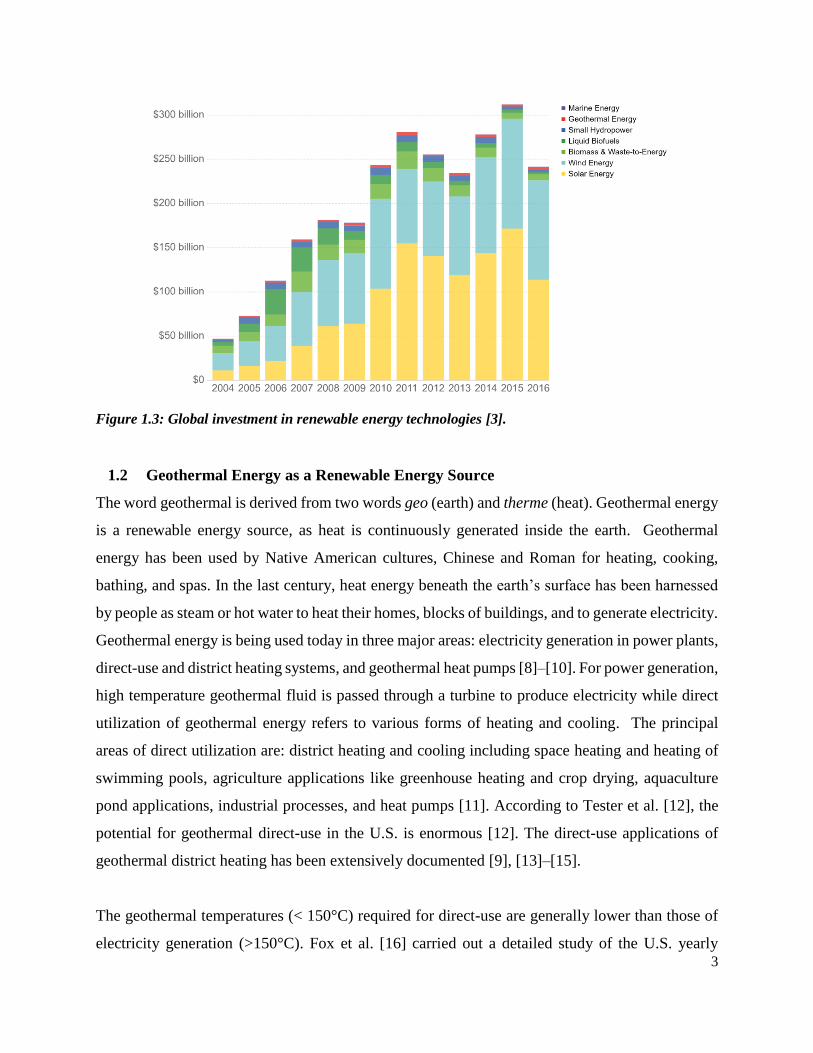
For example there is about 600% increase in the investment in renewable energy between 2004
and 2015 as seen in Figure 1.3 [4], and the major investments are in solar and wind over the past
few years. However, these resources are not available at all times and require costly and
complicated devices to store energy , while geothermal energy is available at all times, more
reliable, easily scalable, and provides a significant amount of energy [5]. Nationally, it has been
estimated geothermal, as of 2007, contributes 0.5% of the total U.S. energy demand [6] and as of
2018, constitutes only 2% of the total renewable energy consumption in the U.S. [7].
3
Figure 1.3: Global investment in renewable energy technologies [3].
1.2 Geothermal Energy as a Renewable Energy Source
The word geothermal is derived from two words geo (earth) and therme (heat). Geothermal energy
is a renewable energy source, as heat is continuously generated inside the earth. Geothermal
energy has been used by Native American cultures, Chinese and Roman for heating, cooking,
bathing, and spas. In the last century, heat energy beneath the earth’s surface has been harnessed
by people as steam or hot water to heat their homes, blocks of buildings, and to generate electricity.
Geothermal energy is being used today in three major areas: electricity generation in power plants,
direct-use and district heating systems, and geothermal heat pumps [8]–[10]. For power generation,
high temperature geothermal fluid is passed through a turbine to produce electricity while direct
utilization of geothermal energy refers to various forms of heating and cooling. The principal
areas of direct utilization are: district heating and cooling including space heating and heating of
swimming pools, agriculture applications like greenhouse heating and crop drying, aquaculture
pond applications, industrial processes, and heat pumps [11]. According to Tester et al. [12], the
potential for geothermal direct-use in the U.S. is enormous [12]. The direct-use applications of
geothermal district heating has been extensively documented [9], [13]–[15].
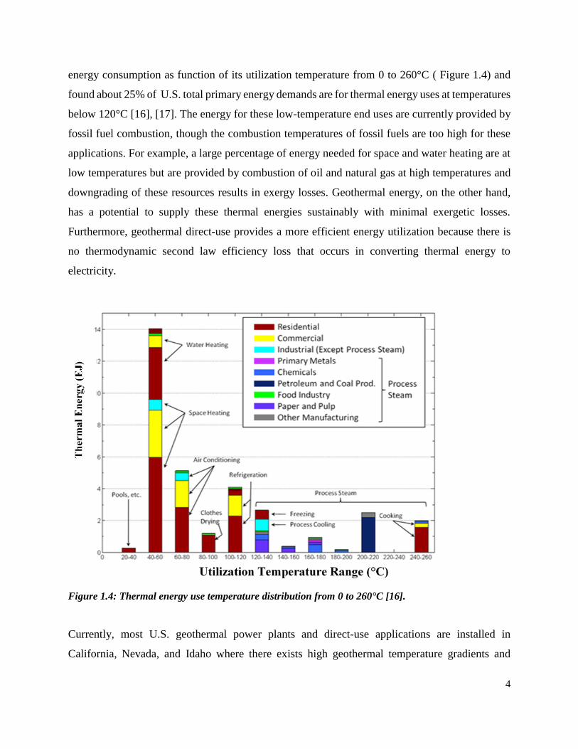
The geothermal temperatures (< 150°C) required for direct-use are generally lower than those of
electricity generation (>150°C). Fox et al. [16] carried out a detailed study of the U.S. yearly
4
energy consumption as function of its utilization temperature from 0 to 260°C ( Figure 1.4) and
found about 25% of U.S. total primary energy demands are for thermal energy uses at temperatures
below 120°C [16], [17]. The energy for these low-temperature end uses are currently provided by
fossil fuel combustion, though the combustion temperatures of fossil fuels are too high for these
applications. For example, a large percentage of energy needed for space and water heating are at
low temperatures but are provided by combustion of oil and natural gas at high temperatures and
downgrading of these resources results in exergy losses. Geothermal energy, on the other hand,
has a potential to supply these thermal energies sustainably with minimal exergetic losses.
Furthermore, geothermal direct-use provides a more efficient energy utilization because there is
no thermodynamic second law efficiency loss that occurs in converting thermal energy to
electricity.
Figure 1.4: Thermal energy use temperature distribution from 0 to 260°C [16].
Currently, most U.S. geothermal power plants and direct-use applications are installed in
California, Nevada, and Idaho where there exists high geothermal temperature gradients and
5
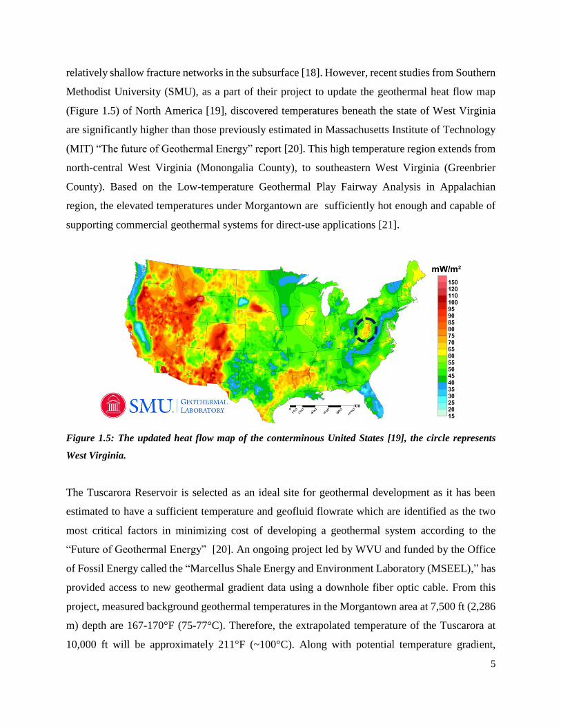
relatively shallow fracture networks in the subsurface [18]. However, recent studies from Southern
Methodist University (SMU), as a part of their project to update the geothermal heat flow map
(Figure 1.5) of North America [19], discovered temperatures beneath the state of West Virginia
are significantly higher than those previously estimated in Massachusetts Institute of Technology
(MIT) “The future of Geothermal Energy” report [20]. This high temperature region extends from
north-central West Virginia (Monongalia County), to southeastern West Virginia (Greenbrier
County). Based on the Low-temperature Geothermal Play Fairway Analysis in Appalachian
region, the elevated temperatures under Morgantown are sufficiently hot enough and capable of
supporting commercial geothermal systems for direct-use applications [21].
Figure 1.5: The updated heat flow map of the conterminous United States [19], the circle represents
West Virginia.
The Tuscarora Reservoir is selected as an ideal site for geothermal development as it has been
estimated to have a sufficient temperature and geofluid flowrate which are identified as the two
most critical factors in minimizing cost of developing a geothermal system according to the
“Future of Geothermal Energy” [20]. An ongoing project led by WVU and funded by the Office
of Fossil Energy called the “Marcellus Shale Energy and Environment Laboratory (MSEEL),” has
provided access to new geothermal gradient data using a downhole fiber optic cable. From this
project, measured background geothermal temperatures in the Morgantown area at 7,500 ft (2,286
m) depth are 167-170°F (75-77°C). Therefore, the extrapolated temperature of the Tuscarora at
10,000 ft will be approximately 211°F (~100°C). Along with potential temperature gradient,

6
significant porosity and permeability is expected, based on resistivity logs and gas production
history in this area. Deep direct-use geothermal development requires an additional critical factor
for economic viability: available thermal demand and appropriate surface distribution
infrastructure. The market for the geothermal resource in Morgantown will be the commercial and
residential sectors of the WVU campus, comprising 1,892 acres; 245 buildings; and 30,000 faculty,
staff, and students. Hence, the WVU campus offers surface demand coupled with potential
subsurface viability.
1.3 Objectives and Approach
The main goal of this project was to perform a feasibility analysis of developing a geothermal
district heating and cooling (GDHC) system for the WVU campus in Morgantown WV to replace
the current coal-fired steam heating and cooling system, which serves over a 30,000 student,
faculty and staff population spread across more than 1,800 acres with 245 campus buildings. The
steam to the campus loop is currently provided by Morgantown Energy Associates (MEA), a coal-
based power plant. The sustainability plan, managed under the Office of Sustainability and the
WVU Energy Institute, aims to advance the efforts of WVU to achieve a reliable and clean energy
source for their central steam generation system. Geothermal is identified as one of the potential
options.
The heating and cooling system at WVU is unique due to the year-round use of steam for heating
in winter and cooling in the summer months using absorption cooling. Therefore, the use of
geothermal heating at WVU would result in year-round utilization of the deep direct-use (DDU)
system, hence lowering the levelized cost of heat (LCOH) by fully amortizing the system over 12
months thus providing the first demonstration of the practical feasibility and effectiveness of a
geothermal system in the eastern U.S.
The specific objectives of this study:
1. Objective 1: Characterize energy demand for the WVU campus. The year-round energy
consumption data of the WVU campus is collected to characterize the energy demand.
2. Objective 2: Evaluate existing campus district heating system retrofit capability.
3. Objective 3: Design a geothermal surface plant and pipeline distribution using Aspen
simulators.
7
4. Objective 4: Perform an economic analysis to estimate the levelized cost of heat (LCOH)
using GEOPHIRES (GEOthermal energy for Production of Heat and electricity (“IR”)
Economically Simulated) [22].
The feasibility of the hybrid GDHC system at WVU was determined by comparing costs and
benefits with the existing MEA coal-fired steam-based system.
1.4 Thesis Structure
In chapter 1, background information about geothermal energy system in U.S. is discussed.
Chapter 2 reviews development of GDHC system in US and provided the overview of the existing
district heating and cooling (DHC) system at the WVU. The first and second objectives make up
chapter 3 of this thesis. In objective 1 data were collected over the project period to provide
information about the temperature, pressure and flow rates from the existing surface facilities,
analysis from objective 2 provides information about the required new set of equipment and
distribution pipelines which are not part of the current surface plant facilities for the coal-fired
steam-based system. Chapter 4 describes geothermal surface plant and distribution pipeline
simulation setup. In chapter 4, the data and new sets of equipment identified from Chapter 3 are
used for the HYSYS simulations. Aspen Exchanger Design and Rating (EDR) and Aspen capital
cost estimator (ACCE) methodologies are also described in chapter 4. In chapter 5, HYSYS
simulation results are presented and the results obtained from HYSYS simulations provide the
inputs required to perform rigorous design in Aspen EDR for geothermal plate heat exchanger and
shell and tube heat exchanger for fuel preheater. Chapter 5 uses Aspen ACCE to provide the costs
associated with the surface plant equipment and distribution pipelines. The main goal of chapter 6
is to perform an economic evaluation of the entire project using GEOPHIRES software and the
resulting levelized cost of heat (LCOH) is used to assess the feasibility of the hybrid GDHC system
at WVU. Furthermore, a comparison is made between natural gas boiler system and a hybrid
geothermal-natural gas system to identify (analyze) which of the two systems could potentially
replace the current MEA coal-fired steam-based system. Chapter 7 provides future directions and
recommendations for further works.
8
Literature Review
2.1 Development of Geothermal District Heating and cooling (GDHC) System in US.
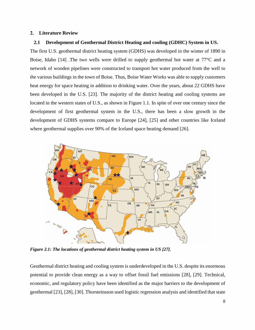
The first U.S. geothermal district heating system (GDHS) was developed in the winter of 1890 in
Boise, Idaho [14] .The two wells were drilled to supply geothermal hot water at 77°C and a
network of wooden pipelines were constructed to transport hot water produced from the well to
the various buildings in the town of Boise. Thus, Boise Water Works was able to supply customers
heat energy for space heating in addition to drinking water. Over the years, about 22 GDHS have
been developed in the U.S. [23]. The majority of the district heating and cooling systems are
located in the western states of U.S., as shown in Figure 1.1. In spite of over one century since the
development of first geothermal system in the U.S., there has been a slow growth in the
development of GDHS systems compare to Europe [24], [25] and other countries like Iceland
where geothermal supplies over 90% of the Iceland space heating demand [26].
Figure 2.1: The locations of geothermal district heating system in US [27].
Geothermal district heating and cooling system is underdeveloped in the U.S. despite its enormous
potential to provide clean energy as a way to offset fossil fuel emissions [28], [29]. Technical,
economic, and regulatory policy have been identified as the major barriers to the development of
geothermal [23], [28], [30]. Thorsteinsson used logistic regression analysis and identified that state
9
funding and design problems were the two most significant variables that influence development
of successful GDHC system in the U.S. [23]. It has been shown that the development of geothermal
district heating system requires a large initial investment in terms of geothermal drilling and
exploration and involves significant risks in drilling a geothermal well [31], [32]. In addition to
the costs of drilling geothermal well, surface plant equipment costs, scaling and corrosion of
equipment, and pipeline infrastructure have been identified to contribute to the barriers for the
development of a geothermal district heating and cooling system in U.S. Consequently, the design
of a district heating and cooling system at WVU is analyzed to ensure successful development of
a GDHC system at WVU.
2.2 Surface Plant Development
A geothermal surface plant can be effectively integrated into the existing district heating and
cooling system by retrofitting existing DHC system to develop a GDHC [33], [34]. Geothermal
heating system is preferably used as the primary source of heat energy in GDHC; but, it could be
combined with other forms of energy to provide additional benefits [35]. Depending on geothermal
fluid production temperatures, it may be beneficial to develop a hybrid DHC system that includes
a heat pump and /or conventional boiler as part of the DHC system design [24], [36]. For example,
in certain district heating systems, geothermal energy is used to provide the base-load energy
demand and a boiler is used to provide peak-load demand during the winter season [37]–[39]. In a
GDHC system where geothermal cannot meet the district heating requirement, fossil fuel (natural
gas) or biomass boiler can be used to provide additional heat required to create a system called
hybrid GDHC system [40], [41]. In some other cases, geothermal energy utilization could be
further improved by using lower-temperature spent geothermal fluid for other purposes including
greenhouse and swimming pool heating called heat cascading or multi-stage utilization where
lower temperatures are used in sequential steps. For other cases, the performance of geothermal
energy utilization in a DHC could be improved by the use of a heat pump system.
10
2.3 Overview of district heating and cooling (DHC) system at WVU
2.3.1 Existing Heating and Cooling System at WVU
The current DHC system at WVU is steam-based. The current system uses steam to heat the water
and the hot water is circulated throughout the buildings for heating and domestic usage, while
some equipment across campuses like absorption cooling towers and autoclaves require steam for
their operation. Ruby Memorial Hospital also requires a significant amount of steam supply for
medical purposes in addition to building heat.
2.3.2 Proposed Heating and Cooling System at WVU
The expected geofluid from the well cannot meet the campus steam demand because geofluid
produced is hot water with temperatures below 100°C. The conversion of steam-based system to
hot water system could be uneconomical and complicated [42]. Therefore, in order to utilize the
existing campus heating and cooling facilities, a hybrid geothermal-natural gas system was
proposed to supply steam at required conditions. The geothermal fluid preheated the condensate
water, which was further heated to required steam conditions using a natural gas boiler. The major
components of the proposed hybrid GDHC system include: a centralized geothermal heat
exchanger to extract geothermal heat, a heat pump system to further extract more heat from low-
temperature return condensate thereby improving the geothermal extraction and performance of
the system, a natural gas boiler to heat hot water to steam, condensate receiver tank, condensate
pumps, and retrofitted pipeline networks to transport secondary fluid from the central plant to
existing pipelines.
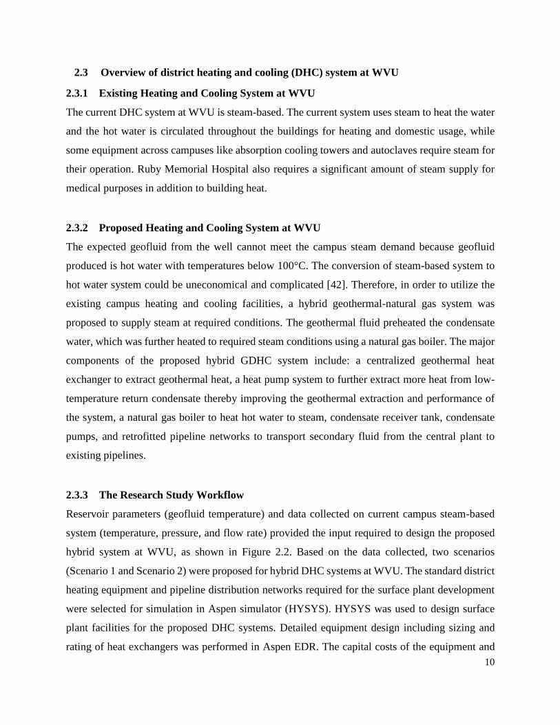
2.3.3 The Research Study Workflow
Reservoir parameters (geofluid temperature) and data collected on current campus steam-based
system (temperature, pressure, and flow rate) provided the input required to design the proposed
hybrid system at WVU, as shown in Figure 2.2. Based on the data collected, two scenarios
(Scenario 1 and Scenario 2) were proposed for hybrid DHC systems at WVU. The standard district
heating equipment and pipeline distribution networks required for the surface plant development
were selected for simulation in Aspen simulator (HYSYS). HYSYS was used to design surface
plant facilities for the proposed DHC systems. Detailed equipment design including sizing and
rating of heat exchangers was performed in Aspen EDR. The capital costs of the equipment and
11
pipelines for the two scenarios were calculated in Aspen ACCE. The total capital costs of
equipment and pipelines are used for economic analysis of the hybrid systems in GEOPHIRES.
The feasibility of hybrid geothermal-natural gas was determined by comparing the LCOH of the
proposed hybrid systems with the existing coal-fired steam-based system. The workflow for the
entire project is summarized in Figure 2.2.
Figure 2.2: A schematic of the workflow for the design and economic analysis of a hybrid GDHC system
at WVU.

12
Characterization of Existing Infrastructure and Evaluation of Existing Campus District
Heating (DH) System Retrofit Capability
3.1 Objective 1: Characterization of Existing Infrastructure
The year-round energy consumption data for the WVU campus buildings was collected to
characterize the energy demand. Currently, MEA supplies steam to five main distribution points
located at three campuses (Downtown, Evansdale and Health Sciences campuses) and the
distribution points supply steam directly to the individual building. Thus, flow meter servers were
installed at distribution points to record steam temperature, pressure, flow rate, and return
condensate flow rate and temperature over a period of one year.
The steam to the campus is distributed through the following five distribution points:
1. Medical Center: Health Sciences campus and Ruby Memorial Hospital
2. Towers: Residential area
3. Evansdale: Engineering and Agriculture buildings
4. Life Sciences: Life Sciences building
5. Downtown: Majority of the campus buildings in downtown area.
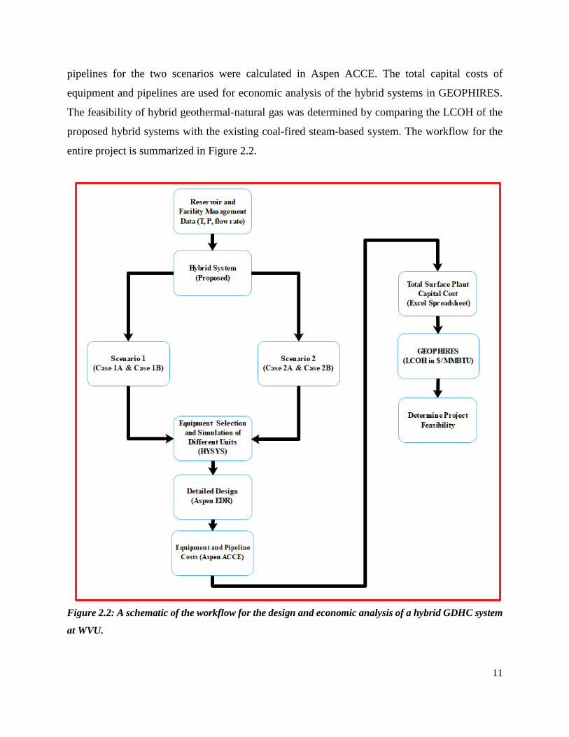
3.2 Objective 1: Results and Discussion
The existing DHS system involves distribution of heat (steam) to 245 buildings from a centralized
coal-fired surface plant owned and operated by MEA. Energy characterization for the three
campuses was based on flow metering data. The flow metering data are recorded or logged in 5-
minute intervals and downloaded monthly to a local computer. The steam flow rates, temperatures,
and pressures obtained were used to characterize energy consumed for the individual campus.
Figure 3.1 shows steam temperature, pressure, and flow rate for Health Sciences campus (Medical
Center meter point) recorded for June 2019.
The annual campus steam consumption for 2017-2018 is shown in Figure 3.2. Steam usage for
three-meter points: Medical center, Evansdale, and Downtown meter points dominates annual
campus steam demand. The figure also shows that steam usage is maximum during the month of
January and minimum during June.
13
Figure 3.1: WVU steam data for (a) temperature (°F) (b) pressure (psig) (c) flow rate (PPH) for Health
Sciences campus (Medical Center meter point) for June 2019.
Figure 3.2: Annual WVU campus steam consumption data for the current DHC system at WVU (2017-
2018).
a)
b)
c)
050
100150200250300350400
6/1/
2019
0:0
06/
1/20
19 1
7:35
6/2/
2019
11:
106/
3/20
19 4
:45
6/3/
2019
22:
206/
4/20
19 1
5:55
6/5/
2019
9:3
06/
6/20
19 3
:05
6/6/
2019
20:
406/
7/20
19 1
4:15
6/8/
2019
7:5
06/
9/20
19 1
:25
6/9/
2019
19:
006/
10/2
019
12:3
56/
11/2
019
6:10
6/11
/201
9 23
:45
6/12
/201
9 17
:20
6/13
/201
9 10
:55
6/14
/201
9 4:
306/
14/2
019
22:0
56/
15/2
019
15:4
06/
16/2
019
9:15
6/17
/201
9 2:
506/
17/2
019
20:2
56/
18/2
019
14:0
06/
19/2
019
7:35
6/20
/201
9 1:
106/
20/2
019
18:4
56/
21/2
019
12:2
06/
22/2
019
5:55
6/22
/201
9 23
:30
6/23
/201
9 17
:05
6/24
/201
9 10
:40
6/25
/201
9 4:
156/
25/2
019
21:5
06/
26/2
019
15:2
56/
27/2
019
9:00
6/28
/201
9 2:
356/
28/2
019
20:1
06/
29/2
019
13:4
56/
30/2
019
7:20
Deg F Avg
84
88
92
96
100
104
108
6/1/
2019
0:0
06/
1/20
19 1
7:35
6/2/
2019
11:
106/
3/20
19 4
:45
6/3/
2019
22:
206/
4/20
19 1
5:55
6/5/
2019
9:3
06/
6/20
19 3
:05
6/6/
2019
20:
406/
7/20
19 1
4:15
6/8/
2019
7:5
06/
9/20
19 1
:25
6/9/
2019
19:
006/
10/2
019
12:3
56/
11/2
019
6:10
6/11
/201
9 23
:45
6/12
/201
9 17
:20
6/13
/201
9 10
:55
6/14
/201
9 4:
306/
14/2
019
22:0
56/
15/2
019
15:4
06/
16/2
019
9:15
6/17
/201
9 2:
506/
17/2
019
20:2
56/
18/2
019
14:0
06/
19/2
019
7:35
6/20
/201
9 1:
106/
20/2
019
18:4
56/
21/2
019
12:2
06/
22/2
019
5:55
6/22
/201
9 23
:30
6/23
/201
9 17
:05
6/24
/201
9 10
:40
6/25
/201
9 4:
156/
25/2
019
21:5
06/
26/2
019
15:2
56/
27/2
019
9:00
6/28
/201
9 2:
356/
28/2
019
20:1
06/
29/2
019
13:4
56/
30/2
019
7:20
PSIG Avg
05000
10000150002000025000300003500040000
6/1/
2019
0:0
06
/1/2
01
9 1
8:0
0
6/2
/20
19
12
:00
6/3/
2019
6:0
06/
4/20
19 0
:00
6/4
/20
19
18
:00
6/5
/20
19
12
:00
6/6
/20
19
6:0
06/
7/20
19 0
:00
6/7/
2019
18:
006
/8/2
01
9 1
2:0
0
6/9
/20
19
6:0
06/
10/2
019
0:00
6/10
/201
9 18
:00
6/1
1/2
01
9 1
2:0
0
6/1
2/2
01
9 6
:00
6/13
/201
9 0:
006/
13/2
019
18:0
06
/14
/20
19
12
:00
6/1
5/2
01
9 6
:00
6/1
6/2
01
9 0
:00
6/16
/201
9 18
:00
6/17
/201
9 12
:00
6/1
8/2
01
9 6
:00
6/1
9/2
01
9 0
:00
6/19
/201
9 18
:00
6/20
/201
9 12
:00
6/2
1/2
01
9 6
:00
6/2
2/2
01
9 0
:00
6/22
/201
9 18
:00
6/23
/201
9 12
:00
6/2
4/2
01
9 6
:00
6/2
5/2
01
9 0
:00
6/2
5/2
01
9 1
8:0
06/
26/2
019
12:0
06/
27/2
019
6:00
6/2
8/2
01
9 0
:00
6/2
8/2
01
9 1
8:0
06/
29/2
019
12:0
06/
30/2
019
6:00
PPH Avg
14
3.3 Objective 2: Evaluate Existing Campus District Heating (DH) System Retrofit
Capability
For the proposed hybrid GDHC system, existing pipeline distribution networks and the equipment
for a DHC system across WVU campuses were evaluated for their retrofit capability. For the
surface plant design, existing building infrastructure will be used. However, new equipment
required at the centralized surface plant location such as a heat exchanger, a natural gas boiler, a
heat pump and a condensate receiver tank to collect return condensate from the five distribution
points were evaluated. The new steam and condensate pipelines required to transport steam and
condensate produced from the central plant site to the existing pipeline distribution system were
identified.
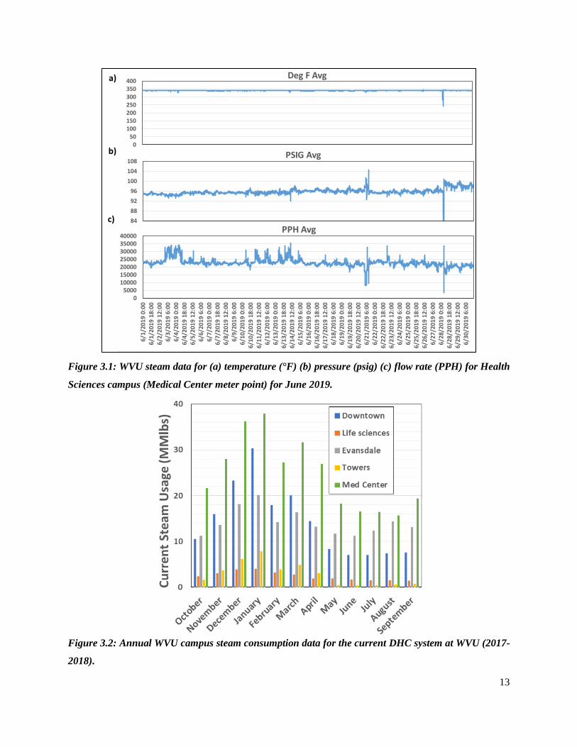
3.4 Objective 2: Results and Discussion
The basic equipment required to meet campus steam requirements were identified. The current
steam supply pipeline networks from MEA, to individual distribution points is shown in Figure
3.3 along with detailed information about the pipe length, pipe diameter, and the locations of the
five distribution points. The pipe lengths are equivalent lengths, which account for bending,
valving, and distribution piping system obstructions.
Figure 3.3: One-line drawing of MEA’s pipelines with distribution meter points along with linear pipe
distances and pipe sizes.
Downtown
126.82 PSIG375.84°F
134.38 PSIG385.98°F
Life Sciences MEA MainTowersAg Sci Med-Center
99.90 PSIG338.14°F
14.74 PSIG274.36°F
~250 PSIG~500°F
505 ft 1996 ft 3945 ft 701 ft 4596 ft
199 ft616 ft700 ft
15
Objective 3: Design a Surface Plant and Pipeline Distribution Using Aspen Simulators
4.1 Proposed Hybrid Geothermal-Natural Gas System Design
The current campus heating and cooling system is steam-based. The expected geofluid from the
well cannot meet the campus steam demand because produced fluid is hot water with temperatures
below 100°C.The current campus heating and cooling system uses steam to heat water and the hot
water produced is circulated within the building for heating and domestic usage, while some
equipment used across campuses like absorption cooling towers and autoclaves require steam for
their operation. Ruby Memorial Hospital also requires a significant amount of steam supply for
medical purposes in addition to building heating. In order to use existing steam-based system, a
hybrid geothermal-natural gas boiler system was proposed for WVU where geothermal fluid was
used to preheat the water and then a natural gas boiler was used to further heat the hot water to
provide steam at required conditions.
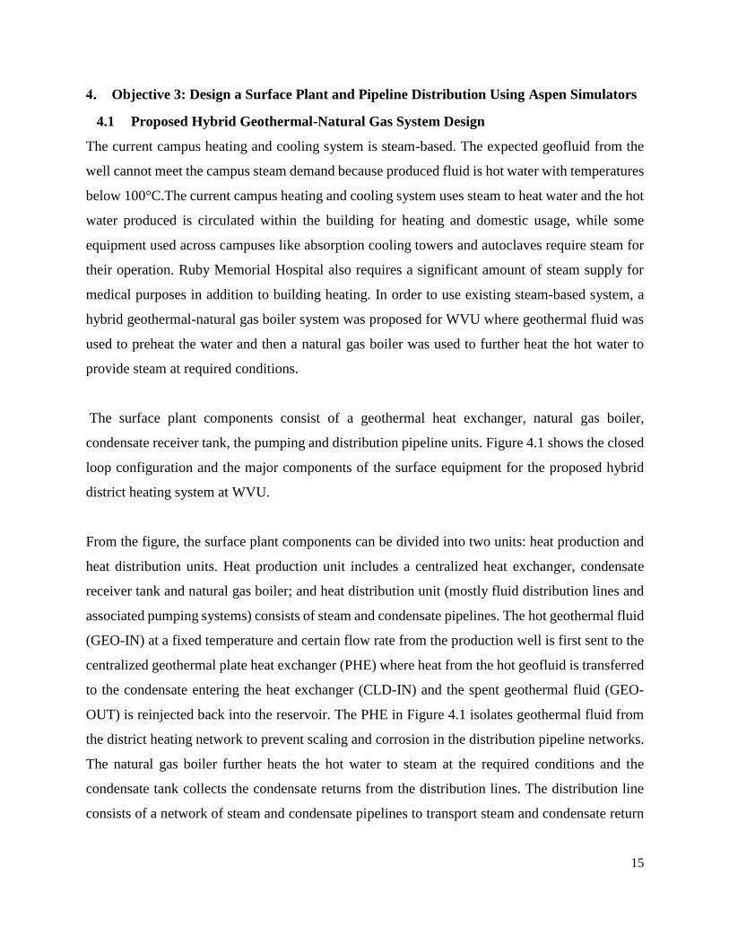
The surface plant components consist of a geothermal heat exchanger, natural gas boiler,
condensate receiver tank, the pumping and distribution pipeline units. Figure 4.1 shows the closed
loop configuration and the major components of the surface equipment for the proposed hybrid
district heating system at WVU.
From the figure, the surface plant components can be divided into two units: heat production and
heat distribution units. Heat production unit includes a centralized heat exchanger, condensate
receiver tank and natural gas boiler; and heat distribution unit (mostly fluid distribution lines and
associated pumping systems) consists of steam and condensate pipelines. The hot geothermal fluid
(GEO-IN) at a fixed temperature and certain flow rate from the production well is first sent to the
centralized geothermal plate heat exchanger (PHE) where heat from the hot geofluid is transferred
to the condensate entering the heat exchanger (CLD-IN) and the spent geothermal fluid (GEO-
OUT) is reinjected back into the reservoir. The PHE in Figure 4.1 isolates geothermal fluid from
the district heating network to prevent scaling and corrosion in the distribution pipeline networks.
The natural gas boiler further heats the hot water to steam at the required conditions and the
condensate tank collects the condensate returns from the distribution lines. The distribution line
consists of a network of steam and condensate pipelines to transport steam and condensate return
16
respectively. To improve heat utilization of the proposed hybrid geothermal-natural gas boiler
system, heat pump system is integrated into the surface plant components in Figure 4.1.
Figure 4.1: Schematic of the proposed hybrid geothermal-natural gas boiler systems for West Virginia
University.
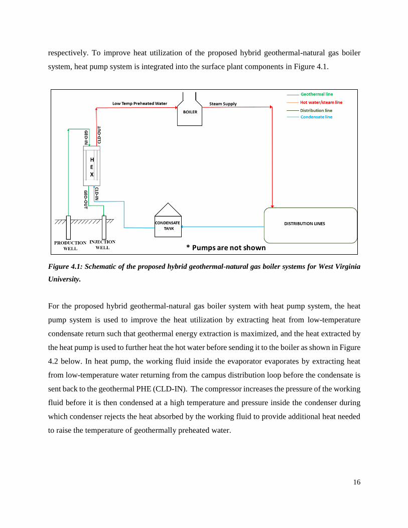
For the proposed hybrid geothermal-natural gas boiler system with heat pump system, the heat
pump system is used to improve the heat utilization by extracting heat from low-temperature
condensate return such that geothermal energy extraction is maximized, and the heat extracted by
the heat pump is used to further heat the hot water before sending it to the boiler as shown in Figure
4.2 below. In heat pump, the working fluid inside the evaporator evaporates by extracting heat
from low-temperature water returning from the campus distribution loop before the condensate is
sent back to the geothermal PHE (CLD-IN). The compressor increases the pressure of the working
fluid before it is then condensed at a high temperature and pressure inside the condenser during
which condenser rejects the heat absorbed by the working fluid to provide additional heat needed
to raise the temperature of geothermally preheated water.
* Pumps are not shown
17
Figure 4.2: Schematic of the proposed hybrid geothermal-natural gas boiler system improvised with heat
pump system for West Virginia University.
High temperature hot water leaving the heat pump system is pressurized by a hot water pump (not
shown in the figure) before it is sent to the natural gas-fired boiler, where it is further heated to
produce steam at required conditions. The steam (superheated or saturated steam) supplied to the
distribution points is sent to individual buildings at WVU for domestic use and heating and cooling
purposes (space heating). As the steam passes through the building, the steam condenses, and the
condensate produced is eventually returned back to respective distribution points. Again, from the
distribution points, a network of condensate pipelines is used to transport the condensate produced
back to the centralized surface plant for re-use by the centralized heat exchanger. The condensate
receiver tank collects all the condensate return to be recirculated back through the loop. For the
distribution lines, a system of condensate pumps is used to re-circulate condensate back to the
central plant site.
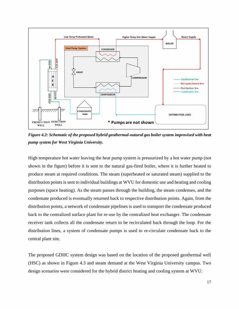
The proposed GDHC system design was based on the location of the proposed geothermal well
(HSC) as shown in Figure 4.3 and steam demand at the West Virginia University campus. Two
design scenarios were considered for the hybrid district heating and cooling system at WVU:
* Pumps are not shown
18
• Scenario 1: supply steam to entire WVU campus (all five distribution points). Scenario 1
involves two cases: Case 1A and Case 1B. In Case 1A, single boiler (Boiler1) provides
high pressure steam at 18.25 bar (250 psig) and 260°C (500°C) to the entire campus while
Case 1B has a boiler (Boiler1) and a compressor. For Case 1B, Boiler1 provides
superheated steam at 14.5 bar (195.6 psig) and 200°C (392°C) to the entire campus except
Life Sciences where the compressor provides superheated steam at 18.25 bar and 260°C to
the Life Sciences meter point.
• Scenario 2: supply steam to Health Sciences (Medical Center meter point) and Evansdale
campuses. Again, Scenario 2 also involves two cases: Case 2A and Case 2B. In Case 2A,
the only boiler (Boiler1) provides saturated steam at 12.5 bar (166.6 psig) to Health
Sciences and Evansdale (Evansdale and Towers meter points) whereas Case 2B has two
boilers; Boiler1 provides saturated steam to Health Sciences and Evansdale meter point at
12.5 bar (166.6 psig) and Boiler2 provides low pressure saturated steam to Towers meter
point at 2.75 bar (25.2 psig).
Figure 4.3: The aerial view of the proposed geothermal well site location at Health Sciences.
19
4.2 Geothermal Heat Exchanger Unit
The objective was to design a geothermal plate heat exchanger that takes in hot geothermal fluid
at 15.2 kg/s for Scenario 1 and 10.2 kg/s for Scenario 2 to heat condensate water. For all cases
considered in this work, a PHE was used to isolate the geothermal fluid because PHE is the most
commonly used in various geothermal applications as geothermal fluid is corrosive and fouling
and hence, the ease of cleaning makes PHE superior to shell and tube heat exchanger (STHE) [43],
[44].
To simulate PHE, first heat exchanger model “Simple End Point” in HYSYS was used to run the
basic simulations. To carry out rigorous design of the PHE and make necessary corrections for
fouling and allowable pressure drop requirements, the process data in HYSYS is exported to Aspen
EDR as in chapter 5. The material of construction is assumed to be stainless steel SS-304 to provide
corrosion resistant to the PHE [43]. For the four cases considered in this work, the process data in
HYSYS is exported to Aspen EDR in chapter 5 where detailed The STHE area, tube passes,
number of tubes, tube pattern, Tubular Exchangers Manufacturers Association (TEMA) shell and
heat types, and estimated shell and tube pressure drops were determined from Aspen EDR rigorous
design. The material of construction is assumed to be carbon steel to provide enough strength for
the high temperature flue gas inlet to the STHE. The simulation run mode in Aspen EDR (chapter
5) is then used to determine the range of values for the allowable pressure drops for the hot and
cold streams which was estimated as 0.02 bar. The estimated pressure drop is used in rigorous
design of the PHE.
Geothermal fluid contains many dissolved chemicals that are corrosive to construction materials.
The chemical composition of a geothermal fluid varies widely and is largely dependent on the
geochemistry of the geothermal reservoir. Although geothermal fluid has a wide variety of
compositions, in this work, the geothermal fluid was assumed to be a pure water and hence,
geothermal fluid was simulated as a pure fluid in HYSYS. Additionally, the built-in fluid property
correlations in GEOPHIRES for density, heat capacity, viscosity, and vapor pressure are based on
the assumption of pure water [45]. However, to account for geothermal fouling of the heat
exchanger, a typical fouling resistance for geothermal fluid (0.0007 ft2-h-°F/BTU) [46] obtained
20
from the literature was used in rigorous design of the heat exchanger. The value for the condensate
fluid fouling resistance (0.0001 ft2-h-°F/BTU) was based on the assumption that the condensate is
a soft water [43].
4.3 Fired heater simulation in HYSYS
The three major sections of the fired heater available in HYSYS (AspenTech) are:
• Radiant Section: consists of a firebox which transfers heat to the heater tubes mainly by
radiation from high-temperature flue gas;
• Convection Section: consists of a bank of tubes which receives heat from the hot flue gases,
primarily by convection; and
• Economizer: used to heat the water fed to the boiler. Economizer is primarily used to
recover heat from the boiler flue gases to increase boiler efficiency.
At steady state, HYSYS fired heater does not have convection and economizer sections. Fired
heater is typically designed with a suitable size, material, and heat of combustion; but, in the case
of this work, HYSYS fired heater simulation is for basic mass and energy balance to provide boiler
heat duty, air-fuel flow rates, and the required steam outlet temperature and pressure at saturated
or super-heated conditions which are required to obtain boiler costs from suitable vendors and to
estimate boiler costs in Aspen ACCE.
Fired heater has four basic components: fire box, burner, convection coil and stack. In the HYSYS
steady state simulation, there is no burner, convection coils, and stack components. Because only
radiative section is active in steady state, no other significant modification or specification was
done for the steady state simulations. Vacuum or negative pressure conditions required for the
boiler operation are not available at steady state; but, the combustion of air and natural gas is
assumed to occur at near atmospheric pressure of about 0.8 bar [47]. For the minimum (lowest)
possible utility cost, the fired heater is assumed to operate at 85% efficiency in order to maximize
fuel usage. This means 85% of the heat is absorbed in the radiant section of the fired heater while
the remaining 15% goes into heating exiting flue gas. Hence, fired heater efficiency for the radiant
section is defined as the ratio of heat supplied to the process fluid to the total heat supplied to the
process fluid and flue gas exiting the stack. Stack consists of a cylindrical brick shell which
21
transports flue gas to the atmosphere and provides necessary draft. As there is no stack section, no
damper is simulated to regulate flue gas flow through the stack or duct and to control draft or
negative pressure (vacuum) in the fired heater as damper is not available for the steady state
simulations. Draft (forced, induced or natural draft), which involves the use of a fan to supply
combustion air to the burner and to overcome the pressure drop through the burner, is simulated
as the air blower in HYSYS. In the HYSYS simulation, natural gas preheater is not available; but
it is simulated using shell and tube heat exchanger where fired heater exiting flue gas is used to
preheat the industrial natural gas supplied before the preheated natural gas enters the fired heater
combustion section (burner).
Factors affecting the performance of the fired heater including the heat burner capacity, air leakage,
negative pressure, economics, and safety are not considered in the steady state simulations. The
flue gas temperature is assumed to be around 385°C [47], [48] which is considered to be high
enough to prevent condensation of the flue gas at dew point.
The objective here was to simulate a natural gas boiler for a given process condition applicable to
the WVU campus district heat supply. The pressure of the preheated water coming from the GEO-
HEX was at 1 bar. However, Scenario 1 and Scenario 2 fired heater simulations require steam
supply at higher pressure conditions in order to meet steam requirements at the distribution points.
To achieve the required steam condition at the distribution points, geothermally preheated high
temperature hot water supply was pumped into the fired heater via a pump (PUMP-1) while natural
gas combustion in the burner provided additional heat energy required to produce superheated
steam (Case 1A & 1B) and saturated steam (Case 2A & 2B). The steam produced was then sent to
the various campuses through a network of underground, buried insulated pipelines which extend
from the centralized surface plant at the well location to the individual campuses. HYSYS
simulated boiler unit is shown in Figure 4.4 below.

22
Figure 4.4: Boiler unit and other combustion components simulated in HYSYS.
In Figure 4.4, fuel preheater (NG-PREHEATER) was used to preheat the natural gas to a desired
temperature before combusted in the boiler and an air blower (AIR-BLOWER) was used to push
air into the combustion chamber. Maintaining natural gas temperature at about 65°C ensures the
combustion is complete.
As shown in Figure 4.4, inlet and outlets streams to the fired heater are:
• PUMP-OUT: geothermal-heat pump preheated water,
• HP-STEAM: saturated or superheated steam produced from combustion of natural gas in
the fired heater,
• Natural Gas and Air-1 (fuel inlets): a mixture of air (dry air) and natural gas, and
• Flue Gas1: Fired heater flue gas exhaust.
The major assumptions and conditions used in fired heater simulation:
• Fired Heater: Firebox efficiency was fixed at 85% and the adjust logical operator in
HYSYS was used to perform optimization at steady state in order to meet steam
requirements at the distribution points.

23
• Air-Fuel Mixture: The air component of the air-fuel mixture for the combustion of natural
gas is assumed to be made up of nitrogen (79%) and oxygen (21%) molar mixture while
natural gas is assumed to be a molar mixture of methane (95%), ethane (2.5%) and propane
(2.5%) [49]. Dry air at 25°C is supplied at 10% excess of the stoichiometric requirement
to ensure complete combustion of natural gas in firebox heater (AspenTech Database).
Natural gas is supplied at industrial delivery pressure of 4.81 bar and a temperature of 15°C
based on current WVU natural gas supply data obtained from WVU Facilities
Management. The combustion of natural gas was assumed to be around atmospheric
conditions and hence, the natural gas pressure was lowered by the valve (LETDOWN).
Finally, a blower was used to push the air into the combustion burner and a fuel preheater
was used to raise industrial natural gas supplied to meet temperature requirement of the
firebox efficiency at 85%.
• Air Blower: Air blower was used to compress and push air into the combustion chamber
of the boiler unit at 0.8 bar
Air and natural gas inlet temperature and pressure for all the boiler units simulated in Aspen
HYSYS are summarized in Table 4-1.
Table 4-1: Air and fuel inlet conditions for fired heater simulation in HYSYS.
Fired Heater Input Air Natural Gas
Temperature (°C) 58.88 63.52
Pressure (bar) 0.80 0.80
Fuel Preheater Unit: Based on the given inlet process conditions for the fired heater, the
efficiency of the fired heater was about 80% whereas it was desired to provide a boiler with an
efficiency as high as 85% to maximize fuel usage. In order to achieve this, the inlet fuel (natural
gas) to the combustion chamber of the boiler was optimized using a fuel preheater. By varying the
natural gas flow rate, adjust operator in HYSYS was used to achieve 85% efficiency in the fired
heater to ensure that steam produced is at the required temperature and the flue gas temperature is
not below 384°C. The fuel preheater optimizes the boiler unit by channeling flue gas (Flue Gas1)
24
exiting the boiler to the heat exchanger (NG-PREHEATER) where the flue gas was used to preheat
the natural gas before it was sent to the boiler unit. STHE were used to obtain the required natural
gas temperature inlet requirement to optimize the boiler. The pressure drop for HYSYS simulation
of simple heat exchanger was assumed to be negligible.
4.4 Distribution Piping System
In geothermal district heating systems, the piping system as well as adequate insulation must be
considered to minimize heat losses through pipelines. The distribution pipeline networks were
used to transport steam produced from surface plant facility to the five distribution points in
Scenario 1 or to the three distribution points in Scenario 2. To determine the total cost of pipeline
distribution networks required to meet heating and cooling demand at WVU, the cost of the
pipelines that transport steam to different campuses at WVU was estimated in Aspen ACCE.
4.4.1 The major assumptions and conditions used in distribution pipeline simulation for
the entire campus include:
• The geothermal well location is near the HSC campus and the existing steam pipeline
network was used for steam distribution. However, new pipelines are added to connect the
geothermal well location at HSC to the existing MEA steam and condensate pipelines.
• One new steam pipeline
o HSCLOT81: transports steam from boiler outlet to the main MEA pipeline that
connects to existing MEA pipeline at the Medical Center meter point.
• Two new condensate pipelines
o Cond-HSCLOT81PIPE-1: transports Evansdale and Downtown condensate return
from main MEA line to the condensate receiver tank at the central plant site.
o Cond-HSCLOT81PIPE-2: transports HSC condensate return from main MEA line
to the condensate receiver tank at the central plant site.
• Fuel pipelines were used to provide natural gas for combustion in the boiler
o NG-PIPE: transports natural gas from industrial delivery location to the boiler unit
at the central plan site.
• Aspen ACCE was used to evaluate pipeline cost for:
25
o Pipe material: carbon steel was used for the natural gas pipeline simulation while
an alloy (carbon steel with chromium) was used to simulate steam and condensate
pipelines in order to prevent pipeline corrosion [50], [51].
o Pipe insulation type: polyurethane
o Pipeline: fully buried
• Other assumptions include:
o No heat loss through the distribution pipelines Q=0
o Pipe surface roughness: 0.00015 ft (AspenTech default value)
o Simulation to check for choke flow condition for all pipelines
o Pipe schedule #: 80
o Water loss between steam and condensate line: 10%
4.4.2 Pipeline Elevation
Because the surface plant location is moved from MEA plant site to a new location at HSC the
elevation changes along the main PRT route were considered for the five distribution points.
Elevation change is defined as change in elevation between any two meter points. Google Maps
was used to obtain the major elevation changes. The pipeline elevation changes along the Personal
Rapid Transport (PRT) lines were input into the pipeline segments in HYSYS simulations. Table
4-2 shows the elevation changes and the corresponding pressure changes along the pipeline
segments that were input into the HYSYS pipeline simulation.
Table 4-2: The elevation changes used in pipeline simulations in HYSYS.
Map Location Pipeline Name Elevation
(ft)
Pressure
(bar)
PRT-BEECHURST to PRT MEA Cond-DTN-LFS2 -111.00 -3.32
PRT MEA to PRT Ag. SC Cond-DTN-LFS 124.00 3.71
PRT Ag. SC to PRT TOWERS Cond-AGDTN -26.00 -0.78
PRT TOWERS to PRT MED CENTER Cond-AGDTNTWRDTN 99.00 2.96
PRT-MEDCENTER to CENTRAL PLANT Cond-HSCLOT81PIPE-1 35.00 1.05
26
4.4.3 Steam distribution pipelines
Figure 4.5 (Scenario 1) and Figure 4.6 (Scenario 2) show that the steam from the boiler outlet
(Figure 4.4) was channeled into the first pipeline HSCLOT81, a new pipeline that connected steam
produced at the centralized surface facility to existing MEA pipelines. At HSCLOT81 exit, the
steam produced was split into two streams: one stream was diverted to the Medical Center meter
point (MED-MTPT), the second stream, was sent to the main MEA steam pipeline at HSC and
was transported to other campuses through a series of existing MEA pipelines. For Scenario 1, the
series of existing MEA steam pipelines were: AGTWRDTN, TWR-PIPE, AG-DTN, AG-PIPE,
DTN-LFSC, DTN-LFSC2, LFS-PIPE, DTN-PIPE while for Scenario 2 (Figure 4.6) the existing
steam pipelines were: AGTWR, TWR-PIPE, AG-MEA, AG-PIPE.
Figure 4.5: The schematic of the steam line simulated for Scenario 1 (Case 1A & Case 1B) pipeline
distribution system.
27
Figure 4.6: The schematic of steam line simulated for Scenario 2 (Case 2A & Case 2B) pipeline
distribution system.
4.4.4 Condensate return pipelines
The pressures of the returning condensate at the distribution points are not known. However, WVU
Facilities Management provided an estimated value of about 3.1 bar (30 psig) for the condensate
pressure leaving an individual building. Assuming a pressure drop of 10 psig between individual
buildings and the meter point, the pressure of the returning condensate entering the meter point
was estimated to be 2.4 bar (20 psig). The entire condensate line was simulated in HYSYS using
2.4 bar as the initial pressure at the meter point for the two scenarios. Also, the condensate flow
rates were regulated such that the total water loss between the steam line supply and condensate
return line was approximately 10%; thus, 90% of the steam supplied was returned as condensate.
The 10% makeup water accounted for water loss in the closed loop system.
Figure 4.7 and Figure 4.8 show the schematic of the condensate pipeline distribution system at
WVU. For Scenario 1 as represented in Figure 4.7, the condensate return was transported from the
28
five distribution points back to the centralized surface facility through existing MEA condensate
pipelines (cond-LFS-PIPE, cond-DTN-PIPE, cond-DTN-LFSC2, cond-LFSC, cond-AG-PIPE,
cond-AG-DTN, cond-TWR-PIPE, cond-AGTWRDTN). Similarly, for Scenario 2 (Figure 4.8) the
condensate return was transported from the three distribution points back to the centralized surface
facility through existing MEA condensate pipelines (cond-AG-PIPE, cond-AG-DTN, cond-TWR-
PIPE, cond-AGDTWRDTN). At HSC, however, two new condensate pipelines were added: cond-
HSCLOT81PIPE-1 and cond-HSCLOT81PIPE-2 for the two scenarios. In Scenario 1 and Scenario
2, the condensate lines delivered their returning water to the heat production unit at 65.59°C and
65.58°C, respectively. The two returning condensate streams were mixed with 10% makeup water
at a temperature of 15°C at a flow rate of 1.52 kg/s for Scenario 1 and at flow rate of 1.02 kg/s for
Scenario 2 before the returning condensate were discharged into the condensate receiver tank
(Figure 4.1). The resulting condensate-makeup water mixture from condensate receiver tank at
48.79°C (Scenario 1) and 50.43°C (Scenario 2) was sent back to GEO-HEX to complete the closed
loop configuration. The condensate tank was assumed to be uninsulated and the residence time for
the condensate return inside the tank was assumed to be negligible.
Figure 4.7: The schematic of the condensate line for Scenario 1 (Case 1A & Case 1B) pipeline
distribution system.
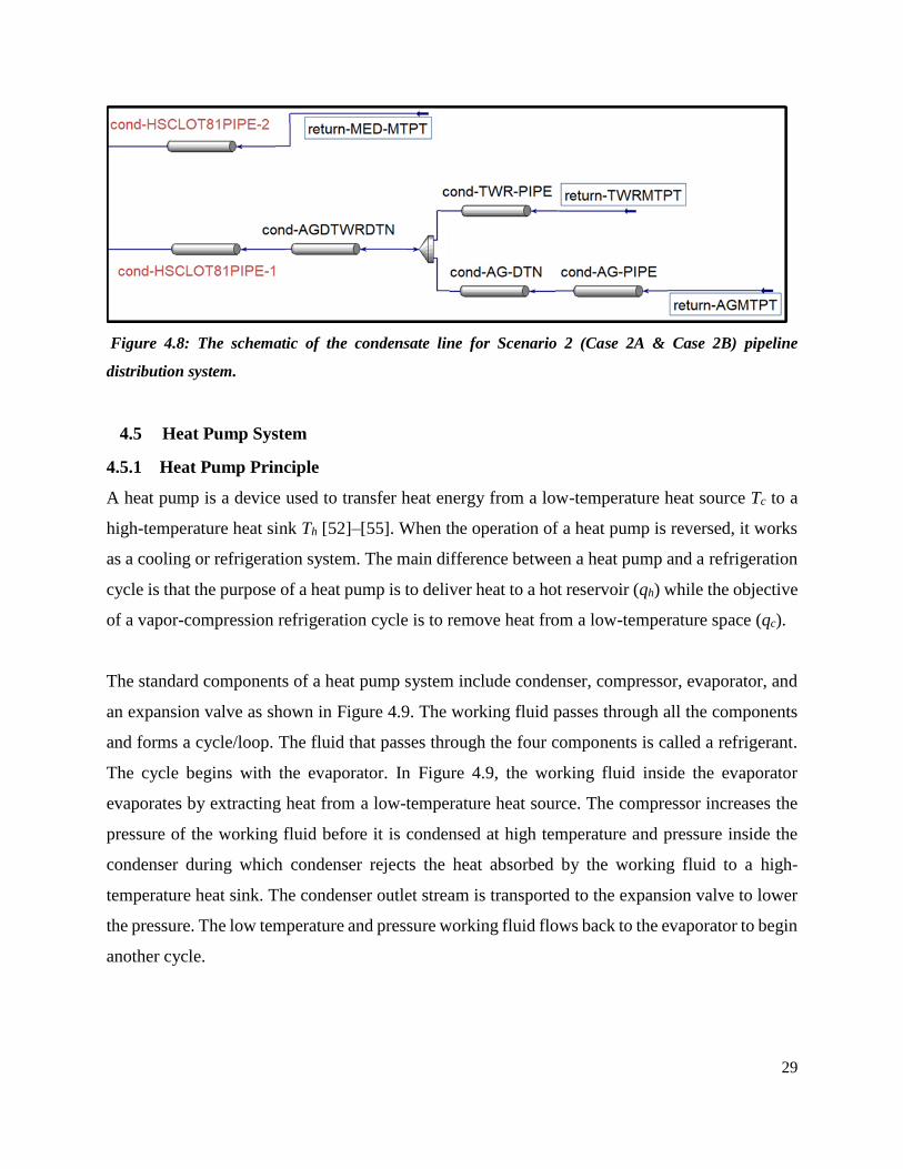
29
Figure 4.8: The schematic of the condensate line for Scenario 2 (Case 2A & Case 2B) pipeline
distribution system.
4.5 Heat Pump System
4.5.1 Heat Pump Principle
A heat pump is a device used to transfer heat energy from a low-temperature heat source Tc to a
high-temperature heat sink Th [52]–[55]. When the operation of a heat pump is reversed, it works
as a cooling or refrigeration system. The main difference between a heat pump and a refrigeration
cycle is that the purpose of a heat pump is to deliver heat to a hot reservoir (qh) while the objective
of a vapor-compression refrigeration cycle is to remove heat from a low-temperature space (qc).
The standard components of a heat pump system include condenser, compressor, evaporator, and
an expansion valve as shown in Figure 4.9. The working fluid passes through all the components
and forms a cycle/loop. The fluid that passes through the four components is called a refrigerant.
The cycle begins with the evaporator. In Figure 4.9, the working fluid inside the evaporator
evaporates by extracting heat from a low-temperature heat source. The compressor increases the
pressure of the working fluid before it is condensed at high temperature and pressure inside the
condenser during which condenser rejects the heat absorbed by the working fluid to a high-
temperature heat sink. The condenser outlet stream is transported to the expansion valve to lower
the pressure. The low temperature and pressure working fluid flows back to the evaporator to begin
another cycle.

30
Efficiency of a heat pump system is expressed by its Coefficient of Performance (COP) [52]. The
COP is calculated as the ratio of the heat rejected by the condenser (qc) to the work input (W) into
the compressor using Eq. 1. The higher the COP, the higher the efficiency of a heat pump system,
𝐶𝑂𝑃ℎ𝑒𝑎𝑡 𝑝𝑢𝑚𝑝 =𝑞𝑐
𝑊 (4.1)
where W is the electric power input into the compressor, and qc is the heat delivered or rejected by
the condenser. The range of COP is usually between 4-6.
Figure 4.9: A simplified diagram of a heat pump system [56].
4.5.2 Selection of working fluid
The design and performance of a heat pump depends on the working fluid employed for its
operation while the efficiency of a heat pump also depends on the difference between heat source
and heat sink temperature. Selection of a working fluid is an important factor as it affects the
operation and efficiency of a heat pump system. Refrigerants such as carbon dioxide (CO2),
ammonia (NH3), water, and hydrocarbons are the commonly used natural working fluid in the heat
pump system operations. Basic simulations were performed for different working fluids and
different heat pump configurations found in the literature. The properties of the working fluid and
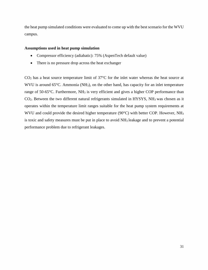
31
the heat pump simulated conditions were evaluated to come up with the best scenario for the WVU
campus.
Assumptions used in heat pump simulation
• Compressor efficiency (adiabatic): 75% (AspenTech default value)
• There is no pressure drop across the heat exchanger
CO2 has a heat source temperature limit of 37°C for the inlet water whereas the heat source at
WVU is around 65°C. Ammonia (NH3), on the other hand, has capacity for an inlet temperature
range of 50-65°C. Furthermore, NH3 is very efficient and gives a higher COP performance than
CO2. Between the two different natural refrigerants simulated in HYSYS, NH3 was chosen as it
operates within the temperature limit ranges suitable for the heat pump system requirements at
WVU and could provide the desired higher temperature (90°C) with better COP. However, NH3
is toxic and safety measures must be put in place to avoid NH3 leakage and to prevent a potential
performance problem due to refrigerant leakages.
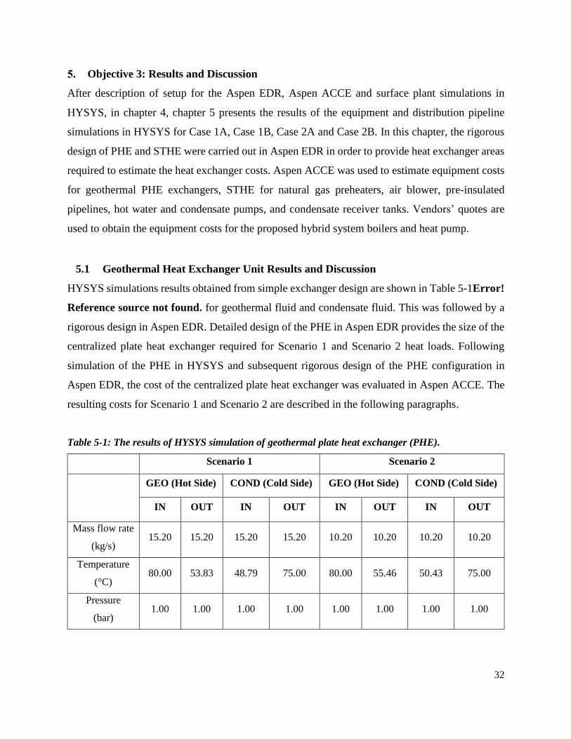
32
Objective 3: Results and Discussion
After description of setup for the Aspen EDR, Aspen ACCE and surface plant simulations in
HYSYS, in chapter 4, chapter 5 presents the results of the equipment and distribution pipeline
simulations in HYSYS for Case 1A, Case 1B, Case 2A and Case 2B. In this chapter, the rigorous
design of PHE and STHE were carried out in Aspen EDR in order to provide heat exchanger areas
required to estimate the heat exchanger costs. Aspen ACCE was used to estimate equipment costs
for geothermal PHE exchangers, STHE for natural gas preheaters, air blower, pre-insulated
pipelines, hot water and condensate pumps, and condensate receiver tanks. Vendors’ quotes are
used to obtain the equipment costs for the proposed hybrid system boilers and heat pump.
5.1 Geothermal Heat Exchanger Unit Results and Discussion
HYSYS simulations results obtained from simple exchanger design are shown in Table 5-1Error!
Reference source not found. for geothermal fluid and condensate fluid. This was followed by a
rigorous design in Aspen EDR. Detailed design of the PHE in Aspen EDR provides the size of the
centralized plate heat exchanger required for Scenario 1 and Scenario 2 heat loads. Following
simulation of the PHE in HYSYS and subsequent rigorous design of the PHE configuration in
Aspen EDR, the cost of the centralized plate heat exchanger was evaluated in Aspen ACCE. The
resulting costs for Scenario 1 and Scenario 2 are described in the following paragraphs.
Table 5-1: The results of HYSYS simulation of geothermal plate heat exchanger (PHE).
Scenario 1 Scenario 2
GEO (Hot Side) COND (Cold Side) GEO (Hot Side) COND (Cold Side)
IN OUT IN OUT IN OUT IN OUT
Mass flow rate
(kg/s) 15.20 15.20 15.20 15.20 10.20 10.20 10.20 10.20
Temperature
(°C) 80.00 53.83 48.79 75.00 80.00 55.46 50.43 75.00
Pressure
(bar) 1.00 1.00 1.00 1.00 1.00 1.00 1.00 1.00

33
5.1.1 Scenario 1 Heat Exchanger:
Heat exchanger cost was determined for a centralized system where the entire geothermal district
heating and cooling system has only one heat exchanger centralized at a location. Given a
geothermal hot water flow rate of 15.2 kg/s flowing counter-currently with a condensate water
flow rate (15.2 kg/s), a PHE area of 303.3 m2 is required to transfer about 1.67 MW of heat from
the geothermal fluid to condensate water. The overall heat transfer coefficient of about 1,103
W/m2-K is within the acceptable ranges for plate heat exchanger [57]. Table 5-1 shows PHE
geometry configuration obtained for scenario 1 from rigorous heat exchanger design together with
given inlet and outlet temperatures for the geothermal fluid and condensate water. Table 5-2 shows
the result of the rigorous PHE design in Aspen EDR. The area obtained from the rigorous design
of PHE in EDR was input into Aspen ACCE to estimate cost of the heat exchanger as $221,600.
Figure 5.1: Details of the geometry obtained for Scenario 1 from rigorous heat exchanger design in
EDR.
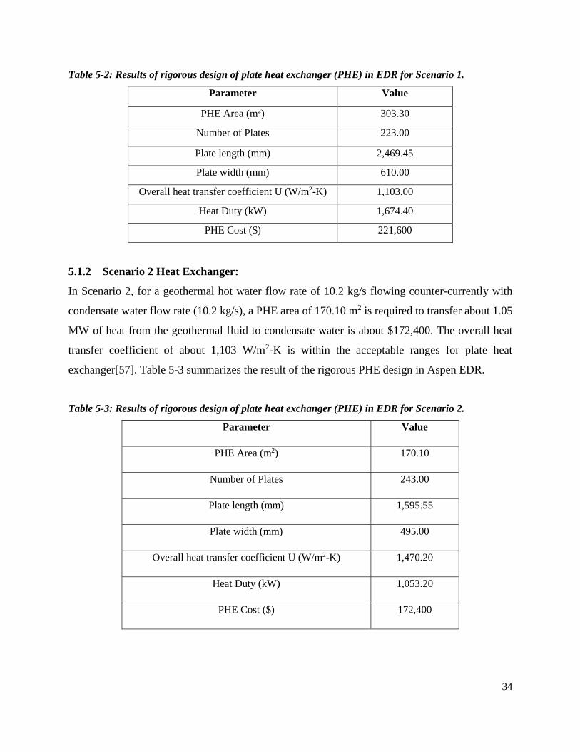
34
Table 5-2: Results of rigorous design of plate heat exchanger (PHE) in EDR for Scenario 1.
Parameter Value
PHE Area (m2) 303.30
Number of Plates 223.00
Plate length (mm) 2,469.45
Plate width (mm) 610.00
Overall heat transfer coefficient U (W/m2-K) 1,103.00
Heat Duty (kW) 1,674.40
PHE Cost ($) 221,600
5.1.2 Scenario 2 Heat Exchanger:
In Scenario 2, for a geothermal hot water flow rate of 10.2 kg/s flowing counter-currently with
condensate water flow rate (10.2 kg/s), a PHE area of 170.10 m2 is required to transfer about 1.05
MW of heat from the geothermal fluid to condensate water is about $172,400. The overall heat
transfer coefficient of about 1,103 W/m2-K is within the acceptable ranges for plate heat
exchanger[57]. Table 5-3 summarizes the result of the rigorous PHE design in Aspen EDR.
Table 5-3: Results of rigorous design of plate heat exchanger (PHE) in EDR for Scenario 2.
Parameter Value
PHE Area (m2) 170.10
Number of Plates 243.00
Plate length (mm) 1,595.55
Plate width (mm) 495.00
Overall heat transfer coefficient U (W/m2-K) 1,470.20
Heat Duty (kW) 1,053.20
PHE Cost ($) 172,400
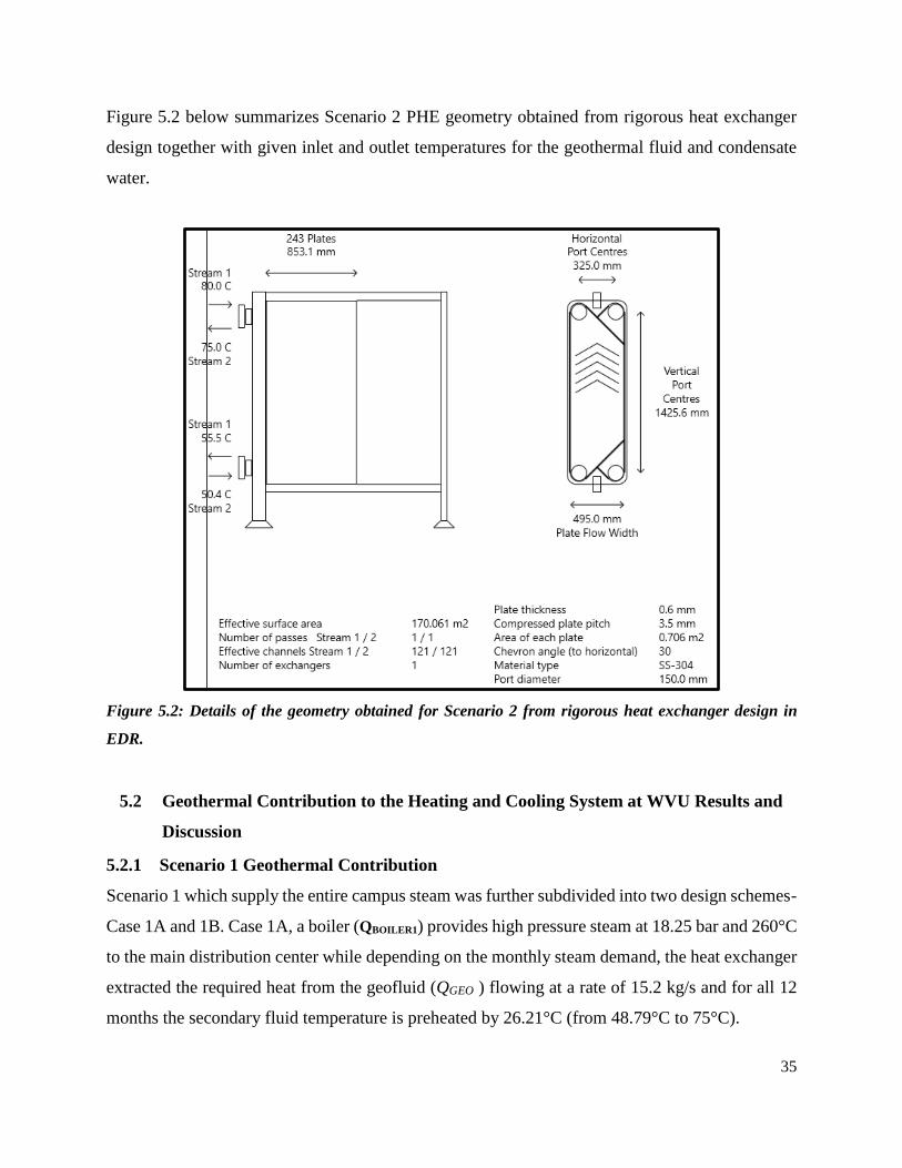
35
Figure 5.2 below summarizes Scenario 2 PHE geometry obtained from rigorous heat exchanger
design together with given inlet and outlet temperatures for the geothermal fluid and condensate
water.
Figure 5.2: Details of the geometry obtained for Scenario 2 from rigorous heat exchanger design in
EDR.
5.2 Geothermal Contribution to the Heating and Cooling System at WVU Results and
Discussion
5.2.1 Scenario 1 Geothermal Contribution
Scenario 1 which supply the entire campus steam was further subdivided into two design schemes-
Case 1A and 1B. Case 1A, a boiler (QBOILER1) provides high pressure steam at 18.25 bar and 260°C
to the main distribution center while depending on the monthly steam demand, the heat exchanger
extracted the required heat from the geofluid (QGEO ) flowing at a rate of 15.2 kg/s and for all 12
months the secondary fluid temperature is preheated by 26.21°C (from 48.79°C to 75°C).
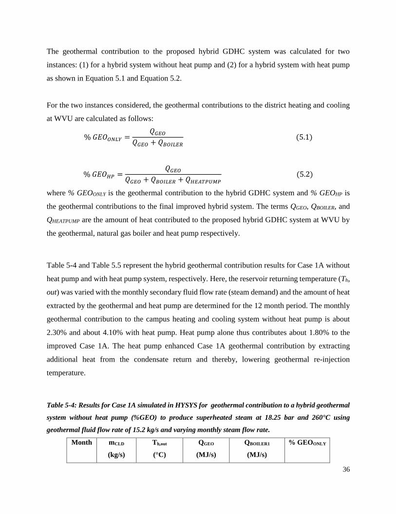
36
The geothermal contribution to the proposed hybrid GDHC system was calculated for two
instances: (1) for a hybrid system without heat pump and (2) for a hybrid system with heat pump
as shown in Equation 5.1 and Equation 5.2.
For the two instances considered, the geothermal contributions to the district heating and cooling
at WVU are calculated as follows:
% 𝐺𝐸𝑂𝑂𝑁𝐿𝑌 =𝑄𝐺𝐸𝑂
𝑄𝐺𝐸𝑂 + 𝑄𝐵𝑂𝐼𝐿𝐸𝑅 (5.1)
% 𝐺𝐸𝑂𝐻𝑃 =𝑄𝐺𝐸𝑂
𝑄𝐺𝐸𝑂 + 𝑄𝐵𝑂𝐼𝐿𝐸𝑅 + 𝑄𝐻𝐸𝐴𝑇𝑃𝑈𝑀𝑃 (5.2)
where % GEOONLY is the geothermal contribution to the hybrid GDHC system and % GEOHP is
the geothermal contributions to the final improved hybrid system. The terms QGEO, QBOILER, and
QHEATPUMP are the amount of heat contributed to the proposed hybrid GDHC system at WVU by
the geothermal, natural gas boiler and heat pump respectively.
Table 5-4 and Table 5.5 represent the hybrid geothermal contribution results for Case 1A without
heat pump and with heat pump system, respectively. Here, the reservoir returning temperature (Th,
out) was varied with the monthly secondary fluid flow rate (steam demand) and the amount of heat
extracted by the geothermal and heat pump are determined for the 12 month period. The monthly
geothermal contribution to the campus heating and cooling system without heat pump is about
2.30% and about 4.10% with heat pump. Heat pump alone thus contributes about 1.80% to the
improved Case 1A. The heat pump enhanced Case 1A geothermal contribution by extracting
additional heat from the condensate return and thereby, lowering geothermal re-injection
temperature.
Table 5-4: Results for Case 1A simulated in HYSYS for geothermal contribution to a hybrid geothermal
system without heat pump (%GEO) to produce superheated steam at 18.25 bar and 260°C using
geothermal fluid flow rate of 15.2 kg/s and varying monthly steam flow rate.
Month mCLD
(kg/s)
Th,out
(°C)
QGEO
(MJ/s)
QBOILER1
(MJ/s)
% GEOONLY
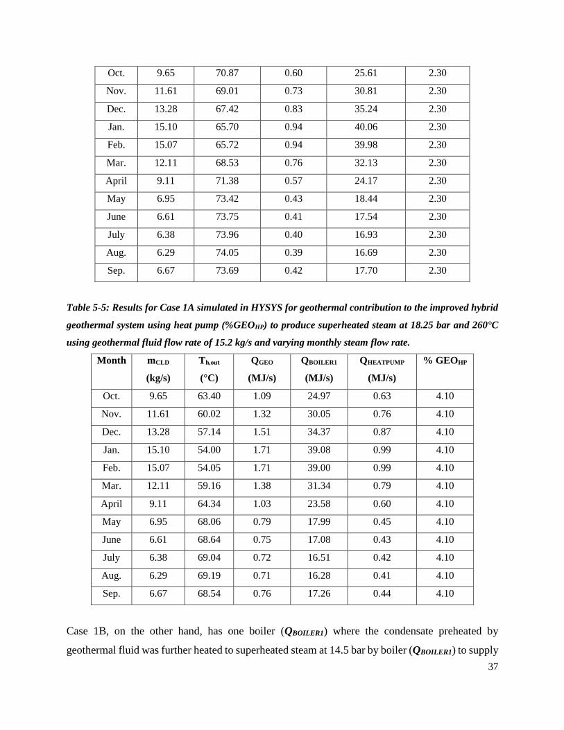
37
Oct. 9.65 70.87 0.60 25.61 2.30
Nov. 11.61 69.01 0.73 30.81 2.30
Dec. 13.28 67.42 0.83 35.24 2.30
Jan. 15.10 65.70 0.94 40.06 2.30
Feb. 15.07 65.72 0.94 39.98 2.30
Mar. 12.11 68.53 0.76 32.13 2.30
April 9.11 71.38 0.57 24.17 2.30
May 6.95 73.42 0.43 18.44 2.30
June 6.61 73.75 0.41 17.54 2.30
July 6.38 73.96 0.40 16.93 2.30
Aug. 6.29 74.05 0.39 16.69 2.30
Sep. 6.67 73.69 0.42 17.70 2.30
Table 5-5: Results for Case 1A simulated in HYSYS for geothermal contribution to the improved hybrid
geothermal system using heat pump (%GEOHP) to produce superheated steam at 18.25 bar and 260°C
using geothermal fluid flow rate of 15.2 kg/s and varying monthly steam flow rate.
Month mCLD
(kg/s)
Th,out
(°C)
QGEO
(MJ/s)
QBOILER1
(MJ/s)
QHEATPUMP
(MJ/s)
% GEOHP
Oct. 9.65 63.40 1.09 24.97 0.63 4.10
Nov. 11.61 60.02 1.32 30.05 0.76 4.10
Dec. 13.28 57.14 1.51 34.37 0.87 4.10
Jan. 15.10 54.00 1.71 39.08 0.99 4.10
Feb. 15.07 54.05 1.71 39.00 0.99 4.10
Mar. 12.11 59.16 1.38 31.34 0.79 4.10
April 9.11 64.34 1.03 23.58 0.60 4.10
May 6.95 68.06 0.79 17.99 0.45 4.10
June 6.61 68.64 0.75 17.08 0.43 4.10
July 6.38 69.04 0.72 16.51 0.42 4.10
Aug. 6.29 69.19 0.71 16.28 0.41 4.10
Sep. 6.67 68.54 0.76 17.26 0.44 4.10
Case 1B, on the other hand, has one boiler (QBOILER1) where the condensate preheated by
geothermal fluid was further heated to superheated steam at 14.5 bar by boiler (QBOILER1) to supply

38
superheated steam at these conditions directly to Health sciences (Medical Center), Evansdale and
Downtown campuses. While at Downtown, the stream to Life Sciences distribution point was
further compressed by a compressor to 18.25 bar for Life Sciences meter point. Based on
geothermal flow rate of 15.2 kg/s and preheating secondary fluid by 26.21°C (from 48.79°C to
75°C), geothermal fluid contributes about 2.40% to the hybrid heating and cooling system as
shown in Table 5.6. After improvement of the hybrid system by the heat pump, Case 1B
geothermal contribution increases from 2.40% to about 4.39% as shown in Table 5.7.
Table 5-6: Results for Case 1B simulated in HYSYS for geothermal contribution to a hybrid geothermal
system without heat pump (%GEO) to produce superheated steam at 14.25 bar and 200°C for Med-
Center, Towers, Evansdale, and Downtown meter points, and the compressor producing superheated
steam at 18.25 bar and 260°C for Life Sciences meter point using geothermal fluid flow rate of 15.2 kg/s.
Month mCLD
(kg/s)
Th,out
(°C)
QGEO
(MJ/s)
QBOILER
(MJ/s)
QCOMP
(MJ/s)
% GEOONLY
Oct. 9.65 70.87 0.60 24.49 0.03 2.40
Nov. 11.61 69.01 0.73 29.46 0.05 2.40
Dec. 13.28 67.42 0.83 33.70 0.06 2.40
Jan. 15.10 65.7 0.94 38.32 0.09 2.40
Feb. 15.07 65.72 0.94 38.32 0.09 2.40
Mar. 12.11 68.53 0.76 30.73 0.05 2.40
April 9.11 71.38 0.57 23.12 0.03 2.40
May 6.95 73.42 0.43 17.64 0.02 2.40
June 6.61 73.75 0.41 16.77 0.02 2.40
July 6.38 73.96 0.40 16.19 0.02 2.40
Aug. 6.29 74.05 0.39 15.96 0.02 2.40
Sep. 6.67 73.69 0.42 16.93 0.02 2.40
Table 5-7: Results for Case 1B simulated in HYSYS for geothermal contribution to the improved hybrid
geothermal system using heat pump (%GEOHP) to produce superheated steam at 14.25 bar and 200°C
for Med-Center, Towers, Evansdale, and Downtown meter points, and the compressor producing
superheated steam at 18.25 bar and 260°C for Life Sciences meter point using geothermal fluid flow rate
of 15.2 kg/s.
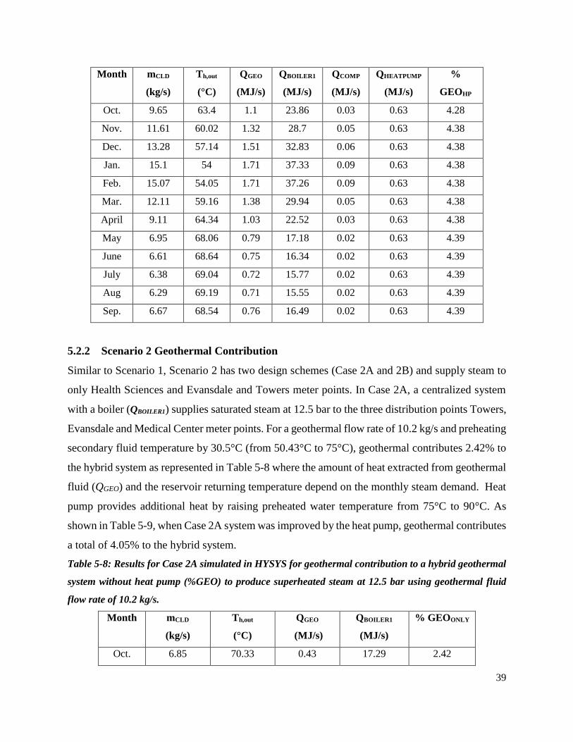
39
Month mCLD
(kg/s)
Th,out
(°C)
QGEO
(MJ/s)
QBOILER1
(MJ/s)
QCOMP
(MJ/s)
QHEATPUMP
(MJ/s)
%
GEOHP
Oct. 9.65 63.4 1.1 23.86 0.03 0.63 4.28
Nov. 11.61 60.02 1.32 28.7 0.05 0.63 4.38
Dec. 13.28 57.14 1.51 32.83 0.06 0.63 4.38
Jan. 15.1 54 1.71 37.33 0.09 0.63 4.38
Feb. 15.07 54.05 1.71 37.26 0.09 0.63 4.38
Mar. 12.11 59.16 1.38 29.94 0.05 0.63 4.38
April 9.11 64.34 1.03 22.52 0.03 0.63 4.38
May 6.95 68.06 0.79 17.18 0.02 0.63 4.39
June 6.61 68.64 0.75 16.34 0.02 0.63 4.39
July 6.38 69.04 0.72 15.77 0.02 0.63 4.39
Aug 6.29 69.19 0.71 15.55 0.02 0.63 4.39
Sep. 6.67 68.54 0.76 16.49 0.02 0.63 4.39
5.2.2 Scenario 2 Geothermal Contribution
Similar to Scenario 1, Scenario 2 has two design schemes (Case 2A and 2B) and supply steam to
only Health Sciences and Evansdale and Towers meter points. In Case 2A, a centralized system
with a boiler (QBOILER1) supplies saturated steam at 12.5 bar to the three distribution points Towers,
Evansdale and Medical Center meter points. For a geothermal flow rate of 10.2 kg/s and preheating
secondary fluid temperature by 30.5°C (from 50.43°C to 75°C), geothermal contributes 2.42% to
the hybrid system as represented in Table 5-8 where the amount of heat extracted from geothermal
fluid (QGEO) and the reservoir returning temperature depend on the monthly steam demand. Heat
pump provides additional heat by raising preheated water temperature from 75°C to 90°C. As
shown in Table 5-9, when Case 2A system was improved by the heat pump, geothermal contributes
a total of 4.05% to the hybrid system.
Table 5-8: Results for Case 2A simulated in HYSYS for geothermal contribution to a hybrid geothermal
system without heat pump (%GEO) to produce superheated steam at 12.5 bar using geothermal fluid
flow rate of 10.2 kg/s.
Month mCLD
(kg/s)
Th,out
(°C)
QGEO
(MJ/s)
QBOILER1
(MJ/s)
% GEOONLY
Oct. 6.85 70.33 0.43 17.29 2.42

40
Nov. 7.83 68.94 0.49 19.76 2.42
Dec. 8.95 67.35 0.56 22.59 2.42
Jan. 10.05 65.79 0.63 25.36 2.42
Feb. 10.02 65.84 0.63 25.36 2.42
Mar. 8.34 68.22 0.52 21.05 2.42
April 6.49 70.83 0.41 16.38 2.42
May 5.08 72.83 0.32 12.82 2.42
June 4.81 73.21 0.30 12.14 2.42
July 4.84 73.17 0.30 12.22 2.42
Aug. 4.78 73.25 0.30 12.06 2.42
Sept. 4.91 73.07 0.31 12.39 2.42
Table 5-9: Results for Case 2A simulated in HYSYS for geothermal contribution to the improved hybrid
geothermal system using heat pump (%GEOHP) to produce superheated steam at 12.5 bar using
geothermal fluid flow rate of 10.2 kg/s.
Month mCLD
(kg/s)
Th,out
(°C)
QGEO
(MJ/s)
QBOILER1
(MJ/s)
QHEATPUMP
(MJ/s)
% GEOHP
Oct. 6.85 63.54 0.73 16.84 0.45 4.05
Nov. 7.83 61.18 0.83 19.25 0.51 4.05
Dec. 8.95 58.48 0.95 22.00 0.59 4.05
Jan. 10.05 55.83 1.07 24.71 0.66 4.05
Feb. 10.02 55.90 1.07 24.63 0.66 4.05
Mar. 8.34 59.95 0.89 20.50 0.55 4.05
April 6.49 64.41 0.69 15.95 0.42 4.05
May 5.08 67.80 0.54 12.49 0.33 4.05
June 4.81 68.45 0.51 11.82 0.31 4.05
July 4.84 68.38 0.52 11.90 0.32 4.05
Aug. 4.78 68.52 0.51 11.75 0.31 4.05
Sep. 4.91 68.21 0.52 12.07 0.32 4.05
Case 2B also has a centralized geothermal heat exchanger but with two boilers. One of the boilers
(QBOILER1) produces saturated steam at 12.5 bar for Evansdale and Medical Center meter points and
the second boiler (QBOILER1) produces saturated steam at 2.75 bar for Towers meter point because

41
Towers requires steam supply at a very low-pressure condition. Based on geothermal flow rate of
10.2 kg/s and preheating secondary fluid by from 48.79°C to 75°C (24.57°C), the geothermal
contribution to the hybrid system is about 2.43% without the heat pump as in Table 5.10 and about
4.05% with heat pump system as shown in Table 5-11.
Table 5-10: Results for Case 2B for geothermal contribution to a hybrid geothermal system without heat
pump (%GEO) with two boilers: one producing saturated steam at 12.5 bar for Evansdale and Medical
Center meter points, and the second boiler producing low pressure steam at 2.75 bar for Towers using
geothermal fluid flow rate of 10.2 kg/s.
Month mCLD
(kg/s)
Th,out
(°C)
QGEO
(MJ/s)
QBOILER1
(MJ/s)
QBOILER2
(MJ/s)
% GEOONLY
Oct. 6.85 70.33 0.43 16.03 1.23 2.43
Nov. 7.83 68.94 0.49 18.32 1.41 2.43
Dec. 8.95 67.35 0.56 20.94 1.61 2.43
Jan. 10.05 65.80 0.63 23.52 1.81 2.43
Feb. 10.02 65.84 0.63 23.45 1.80 2.43
Mar. 8.34 68.20 0.52 19.52 1.50 2.43
April 6.49 70.83 0.41 15.19 1.17 2.43
May 5.08 72.83 0.32 11.89 0.91 2.43
June 4.81 73.21 0.30 11.26 0.86 2.43
July 4.84 73.17 0.30 11.33 0.87 2.43
Aug. 4.78 73.25 0.30 11.19 0.86 2.43
Sep. 4.91 73.07 0.31 11.49 0.88 2.43
Table 5-11: Results for Case 2B for geothermal contribution to the improved hybrid geothermal system
using heat pump (%GEOHP) with two boilers: one producing saturated steam at 12.5 bar for Evansdale
and Med-Center meter points, and the second boiler producing low pressure steam at 2.75 bar for Towers
using geothermal fluid flow rate of 10.2 kg/s.
Month mCLD
(kg/s)
Th,out
(°C)
QGEO
(MJ/s)
QBOILER1
(MJ/s)
QBOILER2
(MJ/s)
QHEATPUMP
(MJ/s)
% GEOHP
Oct. 6.85 63.57 0.73 15.62 1.20 0.45 4.05
Nov. 7.83 61.22 0.83 17.85 1.37 0.51 4.05
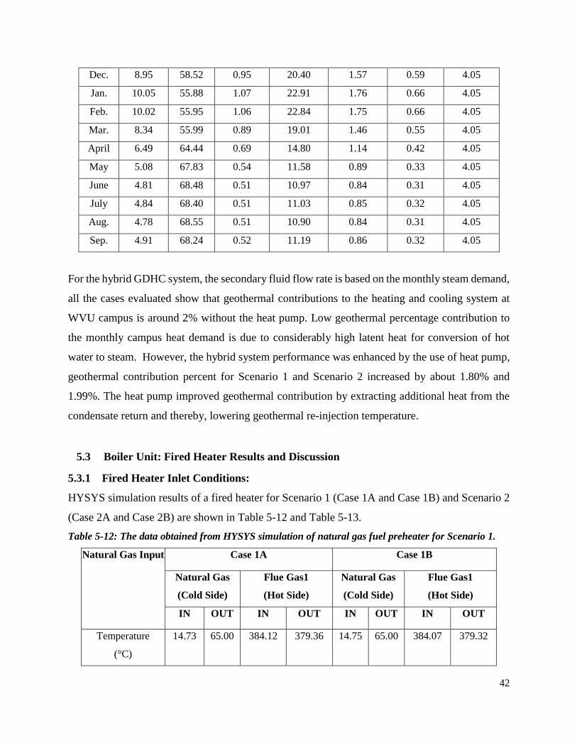
42
Dec. 8.95 58.52 0.95 20.40 1.57 0.59 4.05
Jan. 10.05 55.88 1.07 22.91 1.76 0.66 4.05
Feb. 10.02 55.95 1.06 22.84 1.75 0.66 4.05
Mar. 8.34 55.99 0.89 19.01 1.46 0.55 4.05
April 6.49 64.44 0.69 14.80 1.14 0.42 4.05
May 5.08 67.83 0.54 11.58 0.89 0.33 4.05
June 4.81 68.48 0.51 10.97 0.84 0.31 4.05
July 4.84 68.40 0.51 11.03 0.85 0.32 4.05
Aug. 4.78 68.55 0.51 10.90 0.84 0.31 4.05
Sep. 4.91 68.24 0.52 11.19 0.86 0.32 4.05
For the hybrid GDHC system, the secondary fluid flow rate is based on the monthly steam demand,
all the cases evaluated show that geothermal contributions to the heating and cooling system at
WVU campus is around 2% without the heat pump. Low geothermal percentage contribution to
the monthly campus heat demand is due to considerably high latent heat for conversion of hot
water to steam. However, the hybrid system performance was enhanced by the use of heat pump,
geothermal contribution percent for Scenario 1 and Scenario 2 increased by about 1.80% and
1.99%. The heat pump improved geothermal contribution by extracting additional heat from the
condensate return and thereby, lowering geothermal re-injection temperature.
5.3 Boiler Unit: Fired Heater Results and Discussion
5.3.1 Fired Heater Inlet Conditions:
HYSYS simulation results of a fired heater for Scenario 1 (Case 1A and Case 1B) and Scenario 2
(Case 2A and Case 2B) are shown in Table 5-12 and Table 5-13.
Table 5-12: The data obtained from HYSYS simulation of natural gas fuel preheater for Scenario 1.
Natural Gas Input
Case 1A Case 1B
Natural Gas
(Cold Side)
Flue Gas1
(Hot Side)
Natural Gas
(Cold Side)
Flue Gas1
(Hot Side)
IN OUT IN OUT IN OUT IN OUT
Temperature
(°C)
14.73 65.00 384.12 379.36 14.75 65.00 384.07 379.32
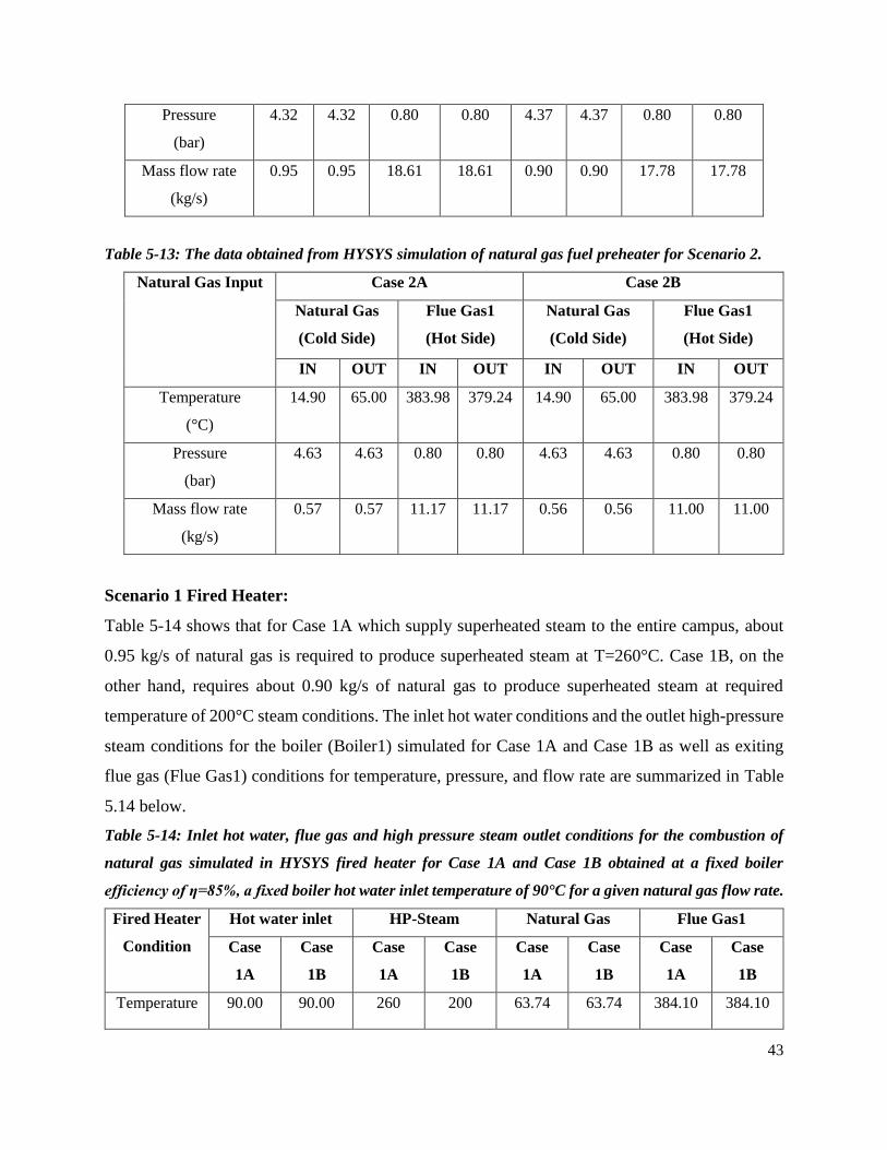
43
Pressure
(bar)
4.32 4.32 0.80 0.80 4.37 4.37 0.80 0.80
Mass flow rate
(kg/s)
0.95 0.95 18.61 18.61 0.90 0.90 17.78 17.78
Table 5-13: The data obtained from HYSYS simulation of natural gas fuel preheater for Scenario 2.
Natural Gas Input
Case 2A Case 2B
Natural Gas
(Cold Side)
Flue Gas1
(Hot Side)
Natural Gas
(Cold Side)
Flue Gas1
(Hot Side)
IN OUT IN OUT IN OUT IN OUT
Temperature
(°C)
14.90 65.00 383.98 379.24 14.90 65.00 383.98 379.24
Pressure
(bar)
4.63 4.63 0.80 0.80 4.63 4.63 0.80 0.80
Mass flow rate
(kg/s)
0.57 0.57 11.17 11.17 0.56 0.56 11.00 11.00
Scenario 1 Fired Heater:
Table 5-14 shows that for Case 1A which supply superheated steam to the entire campus, about
0.95 kg/s of natural gas is required to produce superheated steam at T=260°C. Case 1B, on the
other hand, requires about 0.90 kg/s of natural gas to produce superheated steam at required
temperature of 200°C steam conditions. The inlet hot water conditions and the outlet high-pressure
steam conditions for the boiler (Boiler1) simulated for Case 1A and Case 1B as well as exiting
flue gas (Flue Gas1) conditions for temperature, pressure, and flow rate are summarized in Table
5.14 below.
Table 5-14: Inlet hot water, flue gas and high pressure steam outlet conditions for the combustion of
natural gas simulated in HYSYS fired heater for Case 1A and Case 1B obtained at a fixed boiler
efficiency of η=85%, a fixed boiler hot water inlet temperature of 90°C for a given natural gas flow rate.
Fired Heater
Condition
Hot water inlet HP-Steam Natural Gas Flue Gas1
Case
1A
Case
1B
Case
1A
Case
1B
Case
1A
Case
1B
Case
1A
Case
1B
Temperature 90.00 90.00 260 200 63.74 63.74 384.10 384.10
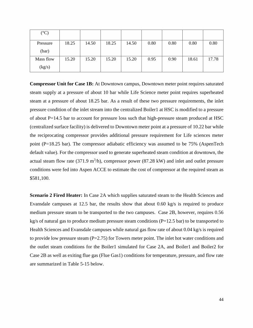
44
(°C)
Pressure
(bar)
18.25 14.50 18.25 14.50 0.80 0.80 0.80 0.80
Mass flow
(kg/s)
15.20 15.20 15.20 15.20 0.95 0.90 18.61 17.78
Compressor Unit for Case 1B: At Downtown campus, Downtown meter point requires saturated
steam supply at a pressure of about 10 bar while Life Science meter point requires superheated
steam at a pressure of about 18.25 bar. As a result of these two pressure requirements, the inlet
pressure condition of the inlet stream into the centralized Boiler1 at HSC is modified to a pressure
of about P=14.5 bar to account for pressure loss such that high-pressure steam produced at HSC
(centralized surface facility) is delivered to Downtown meter point at a pressure of 10.22 bar while
the reciprocating compressor provides additional pressure requirement for Life sciences meter
point (P=18.25 bar). The compressor adiabatic efficiency was assumed to be 75% (AspenTech
default value). For the compressor used to generate superheated steam condition at downtown, the
actual steam flow rate (371.9 m3/h), compressor power (87.28 kW) and inlet and outlet pressure
conditions were fed into Aspen ACCE to estimate the cost of compressor at the required steam as
$581,100.
Scenario 2 Fired Heater: In Case 2A which supplies saturated steam to the Health Sciences and
Evansdale campuses at 12.5 bar, the results show that about 0.60 kg/s is required to produce
medium pressure steam to be transported to the two campuses. Case 2B, however, requires 0.56
kg/s of natural gas to produce medium pressure steam conditions (P=12.5 bar) to be transported to
Health Sciences and Evansdale campuses while natural gas flow rate of about 0.04 kg/s is required
to provide low pressure steam (P=2.75) for Towers meter point. The inlet hot water conditions and
the outlet steam conditions for the Boiler1 simulated for Case 2A, and Boiler1 and Boiler2 for
Case 2B as well as exiting flue gas (Flue Gas1) conditions for temperature, pressure, and flow rate
are summarized in Table 5-15 below.
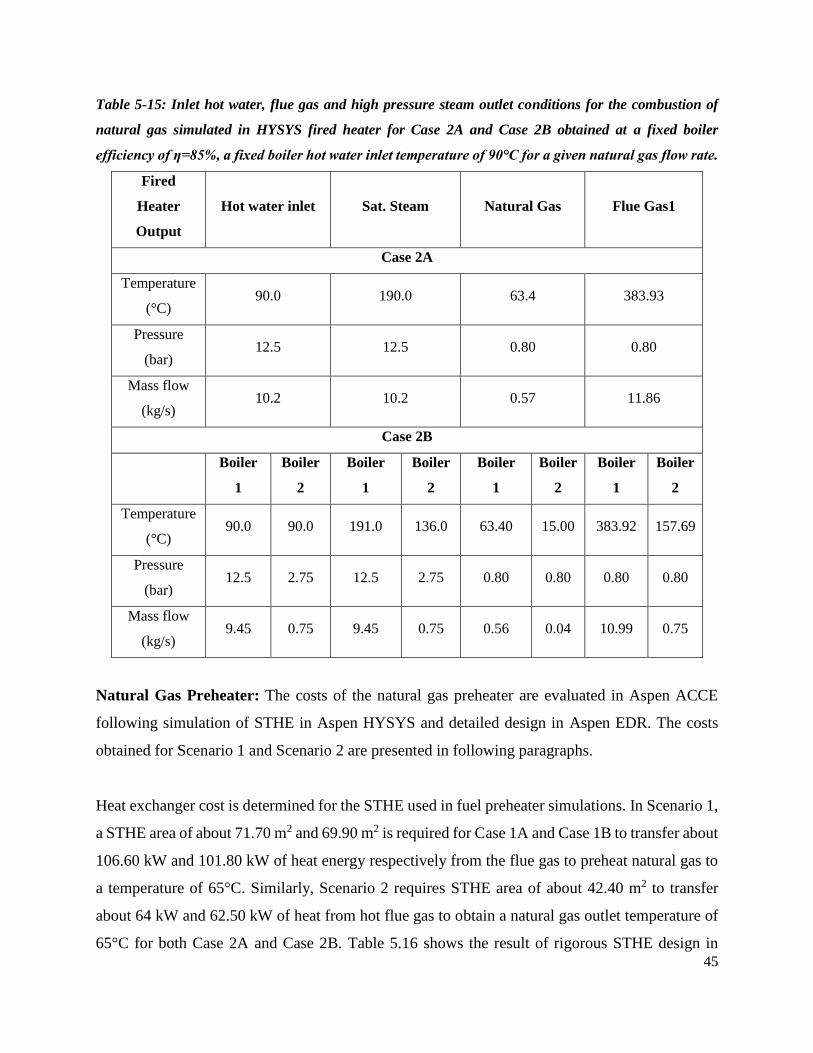
45
Table 5-15: Inlet hot water, flue gas and high pressure steam outlet conditions for the combustion of
natural gas simulated in HYSYS fired heater for Case 2A and Case 2B obtained at a fixed boiler
efficiency of η=85%, a fixed boiler hot water inlet temperature of 90°C for a given natural gas flow rate.
Fired
Heater
Output
Hot water inlet Sat. Steam Natural Gas Flue Gas1
Case 2A
Temperature
(°C) 90.0 190.0 63.4 383.93
Pressure
(bar) 12.5 12.5 0.80 0.80
Mass flow
(kg/s) 10.2 10.2 0.57 11.86
Case 2B
Boiler
1
Boiler
2
Boiler
1
Boiler
2
Boiler
1
Boiler
2
Boiler
1
Boiler
2
Temperature
(°C) 90.0 90.0 191.0 136.0 63.40 15.00 383.92 157.69
Pressure
(bar) 12.5 2.75 12.5 2.75 0.80 0.80 0.80 0.80
Mass flow
(kg/s) 9.45 0.75 9.45 0.75 0.56 0.04 10.99 0.75
Natural Gas Preheater: The costs of the natural gas preheater are evaluated in Aspen ACCE
following simulation of STHE in Aspen HYSYS and detailed design in Aspen EDR. The costs
obtained for Scenario 1 and Scenario 2 are presented in following paragraphs.
Heat exchanger cost is determined for the STHE used in fuel preheater simulations. In Scenario 1,
a STHE area of about 71.70 m2 and 69.90 m2 is required for Case 1A and Case 1B to transfer about
106.60 kW and 101.80 kW of heat energy respectively from the flue gas to preheat natural gas to
a temperature of 65°C. Similarly, Scenario 2 requires STHE area of about 42.40 m2 to transfer
about 64 kW and 62.50 kW of heat from hot flue gas to obtain a natural gas outlet temperature of
65°C for both Case 2A and Case 2B. Table 5.16 shows the result of rigorous STHE design in
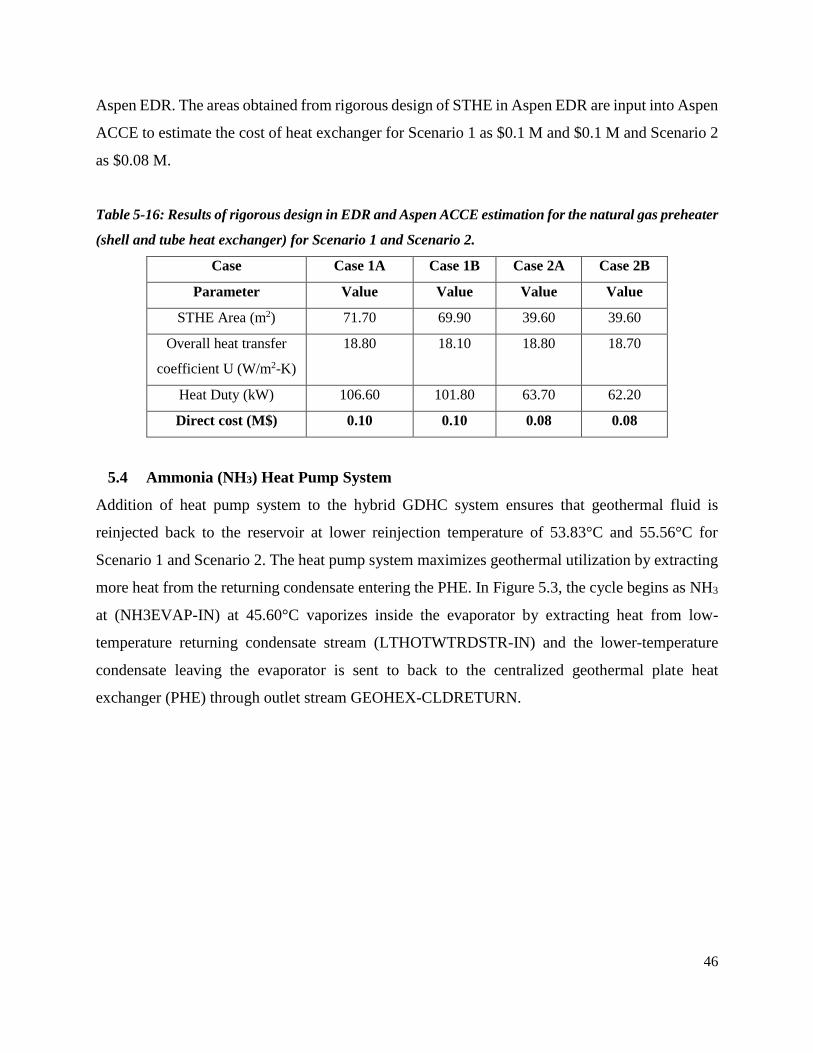
46
Aspen EDR. The areas obtained from rigorous design of STHE in Aspen EDR are input into Aspen
ACCE to estimate the cost of heat exchanger for Scenario 1 as $0.1 M and $0.1 M and Scenario 2
as $0.08 M.
Table 5-16: Results of rigorous design in EDR and Aspen ACCE estimation for the natural gas preheater
(shell and tube heat exchanger) for Scenario 1 and Scenario 2.
Case Case 1A Case 1B Case 2A Case 2B
Parameter Value Value Value Value
STHE Area (m2) 71.70 69.90 39.60 39.60
Overall heat transfer
coefficient U (W/m2-K)
18.80 18.10 18.80 18.70
Heat Duty (kW) 106.60 101.80 63.70 62.20
Direct cost (M$) 0.10 0.10 0.08 0.08
5.4 Ammonia (NH3) Heat Pump System
Addition of heat pump system to the hybrid GDHC system ensures that geothermal fluid is
reinjected back to the reservoir at lower reinjection temperature of 53.83°C and 55.56°C for
Scenario 1 and Scenario 2. The heat pump system maximizes geothermal utilization by extracting
more heat from the returning condensate entering the PHE. In Figure 5.3, the cycle begins as NH3
at (NH3EVAP-IN) at 45.60°C vaporizes inside the evaporator by extracting heat from low-
temperature returning condensate stream (LTHOTWTRDSTR-IN) and the lower-temperature
condensate leaving the evaporator is sent to back to the centralized geothermal plate heat
exchanger (PHE) through outlet stream GEOHEX-CLDRETURN.
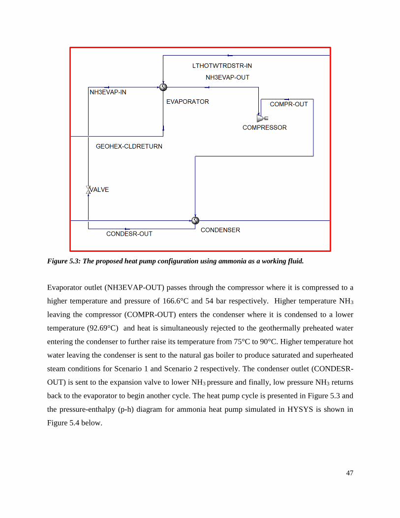
47
Figure 5.3: The proposed heat pump configuration using ammonia as a working fluid.
Evaporator outlet (NH3EVAP-OUT) passes through the compressor where it is compressed to a
higher temperature and pressure of 166.6°C and 54 bar respectively. Higher temperature NH3
leaving the compressor (COMPR-OUT) enters the condenser where it is condensed to a lower
temperature (92.69°C) and heat is simultaneously rejected to the geothermally preheated water
entering the condenser to further raise its temperature from 75°C to 90°C. Higher temperature hot
water leaving the condenser is sent to the natural gas boiler to produce saturated and superheated
steam conditions for Scenario 1 and Scenario 2 respectively. The condenser outlet (CONDESR-
OUT) is sent to the expansion valve to lower NH3 pressure and finally, low pressure NH3 returns
back to the evaporator to begin another cycle. The heat pump cycle is presented in Figure 5.3 and
the pressure-enthalpy (p-h) diagram for ammonia heat pump simulated in HYSYS is shown in
Figure 5.4 below.

48
Figure 5.4: Pressure-enthalpy (p-h) diagram of the ammonia heat pump simulated in HYSYS. The major
components for the heat pump simulated are represented by compressor (1-2), condenser (2-3),
expansion valve (3-4) and evaporator (4-1).
The coefficient of performance (COP) of the heat pump for Scenario 1 and Scenario 2 was
determined. As in equation 4.1, the COP is calculated as the ratio of heat rejected by condenser to
compressor work input obtained for Case 1A, Case1B, Case 2A, and Case 2B are summarized in
Table 5-17 below.
Table 5-17: Results of the coefficient of performance for Scenario 1 and Scenario 2.
Case Compressor
Work (kW)
Condenser Heat
Rejected (kW)
COP
Case 1A 221.33 994.41 4.49
Case 1B 221.33 994.41 4.49
Case 2A 221.33 667.30 3.02
Case 2B 221.33 667.30 3.02

49
The calculated Scenario 1 and Scenario 2 COP are 4.49 and 3.02 respectively. From Table 5-17,
the work input to the compressor is the same for all cases as the working fluid (NH3) flow rate and
temperature entering the compressor from the evaporator are the same for the four cases. However,
the heat rejected by the condenser differs for Scenario 1 and Scenario 2 as the flow rates of heat
absorbing fluid (geothermally preheated water) are different for the two scenarios and hence,
different COP.
5.5 Vendors Quote for Heat Pump and Boiler
Quotes were obtained for boiler unit and heat pump system simulated in HYSYS. The vendor’s
quotes obtained were based on process conditions (steam flow rate) and some design parameters
(design pressure) as summarized in Table 5-18 and Table 5-19 for the boiler and heat pump system
respectively.
5.5.1 Boiler Vendor’s Quote from Johnston Boiler Company (JBC):
The operating pressure (psig), rated capacity (hp), and steam flow rate (lbs/hr) of dry saturated
steam at required pressure obtained from JBC for Scenario 1 and Scenario 2 simulated in HYSYS
are presented in Table 5-18 below.
Table 5-18: Vendor’s quote obtained from Johnston Boiler Company (JBC) for Scenario 1 and Scenario
2 boilers simulated in HYSYS.
Scenario Operating
pressure (psig)
Rated
capacity (hp)
Steam flow
rate (lbs/hr)
Boiler unit
cost ($)
Number
of boilers
Cost
(M$)
Scenario 1
(300#)
250.00 2,000.00 69,000.00 9.12 2 1.83
Scenario 2
(200#)
160.00 2,200.00 75,900.00 8.76 2 1.75
At design pressure of 300 psig, Scenario 1 boiler (300#) is available at a nominal rated capacity of
2,000 hp, 8.69 kg/s (69,000 lbs/hr) and a total of two boilers would be required to meet the existing
meter point steam flow rate flow rate of about 15.2 kg/s (120,636.9 lbs/hr). Scenario 2 boiler
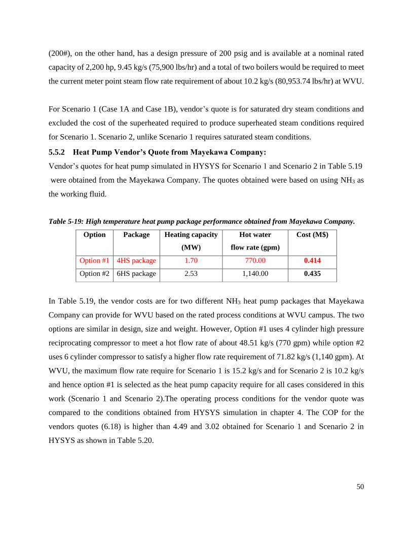
50
(200#), on the other hand, has a design pressure of 200 psig and is available at a nominal rated
capacity of 2,200 hp, 9.45 kg/s (75,900 lbs/hr) and a total of two boilers would be required to meet
the current meter point steam flow rate requirement of about 10.2 kg/s (80,953.74 lbs/hr) at WVU.
For Scenario 1 (Case 1A and Case 1B), vendor’s quote is for saturated dry steam conditions and
excluded the cost of the superheated required to produce superheated steam conditions required
for Scenario 1. Scenario 2, unlike Scenario 1 requires saturated steam conditions.
5.5.2 Heat Pump Vendor’s Quote from Mayekawa Company:
Vendor’s quotes for heat pump simulated in HYSYS for Scenario 1 and Scenario 2 in Table 5.19
were obtained from the Mayekawa Company. The quotes obtained were based on using NH3 as
the working fluid.
Table 5-19: High temperature heat pump package performance obtained from Mayekawa Company.
Option Package Heating capacity
(MW)
Hot water
flow rate (gpm)
Cost (M$)
Option #1 4HS package 1.70 770.00 0.414
Option #2 6HS package 2.53 1,140.00 0.435
In Table 5.19, the vendor costs are for two different NH3 heat pump packages that Mayekawa
Company can provide for WVU based on the rated process conditions at WVU campus. The two
options are similar in design, size and weight. However, Option #1 uses 4 cylinder high pressure
reciprocating compressor to meet a hot flow rate of about 48.51 kg/s (770 gpm) while option #2
uses 6 cylinder compressor to satisfy a higher flow rate requirement of 71.82 kg/s (1,140 gpm). At
WVU, the maximum flow rate require for Scenario 1 is 15.2 kg/s and for Scenario 2 is 10.2 kg/s
and hence option #1 is selected as the heat pump capacity require for all cases considered in this
work (Scenario 1 and Scenario 2).The operating process conditions for the vendor quote was
compared to the conditions obtained from HYSYS simulation in chapter 4. The COP for the
vendors quotes (6.18) is higher than 4.49 and 3.02 obtained for Scenario 1 and Scenario 2 in
HYSYS as shown in Table 5.20.
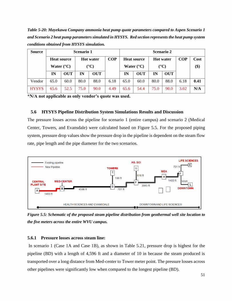
51
Table 5-20: Mayekawa Company ammonia heat pump quote parameters compared to Aspen Scenario 1
and Scenario 2 heat pump parameters simulated in HYSYS. Red section represents the heat pump system
conditions obtained from HYSYS simulation.
Source Scenario 1 Scenario 2
Heat source
Water (°C)
Hot water
(°C)
COP Heat source
Water (°C)
Hot water
(°C)
COP Cost
($)
IN OUT IN OUT IN OUT IN OUT
Vendor 65.0 60.0 80.0 88.0 6.18 65.0 60.0 80.0 88.0 6.18 0.41
HYSYS 65.6 52.5 75.0 90.0 4.49 65.6 54.4 75.0 90.0 3.02 N/A
*N/A not applicable as only vendor’s quote was used.
5.6 HYSYS Pipeline Distribution System Simulations Results and Discussion
The pressure losses across the pipeline for scenario 1 (entire campus) and scenario 2 (Medical
Center, Towers, and Evansdale) were calculated based on Figure 5.5. For the proposed piping
system, pressure drop values show the pressure drop in the pipeline is dependent on the steam flow
rate, pipe length and the pipe diameter for the two scenarios.
Figure 5.5: Schematic of the proposed steam pipeline distribution from geothermal well site location to
the five meters across the entire WVU campus.
5.6.1 Pressure losses across steam line:
In scenario 1 (Case 1A and Case 1B), as shown in Table 5.21, pressure drop is highest for the
pipeline (BD) with a length of 4,596 ft and a diameter of 10 in because the steam produced is
transported over a long distance from Med-center to Tower meter point. The pressure losses across
other pipelines were significantly low when compared to the longest pipeline (BD).
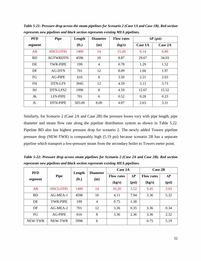
52
Table 5-21: Pressure drop across the steam pipelines for Scenario 2 (Case 1A and Case 1B). Red section
represents new pipelines and black section represents existing MEA pipelines.
PFD
segment
Pipe Length
(ft.)
Diameter
(in)
Flow rates
(kg/s)
ΔP (psi)
Case 1A Case 2A
AB HSCLOT81 1400 14 15.20 6.14 6.80
BD AGTWRDTN 4596 10 8.87 29.67 34.03
DE TWR-PIPE 199 4 0.78 1.29 1.52
DF AG-DTN 701 12 8.09 1.66 1.97
FG AG-PIPE 616 8 3.50 2.21 2.63
FH DTN-LFS 3945 12 4.59 3.13 3.73
HJ DTN-LFS2 1996 8 4.59 12.67 15.52
JK LFS-PIPE 701 6 0.52 0.28 0.23
JL DTN-PIPE 505.00 8.00 4.07 2.63 3.31
Similarly, for Scenario 2 (Case 2A and Case 2B) the pressure losses vary with pipe length, pipe
diameter and steam flow rate along the pipeline distribution system as shown in Table 5.22.
Pipeline BD also has highest pressure drop for scenario 2. The newly added Towers pipeline
pressure drop (NEW-TWR) is comparably high (5.19 psi) because scenario 2B has a separate
pipeline which transport a low-pressure steam from the secondary boiler to Towers meter point.
Table 5-22: Pressure drop across steam pipelines for Scenario 2 (Case 2A and Case 2B). Red section
represents new pipelines and black section represents existing MEA pipelines.
PFD
segment Pipe
Length
(ft.)
Diameter
(in)
Case 2A Case 2B
Flow rates
(kg/s)
ΔP
(psi)
Flow rates
(kg/s)
ΔP
(psi)
AB HSCLOT81 1400 14 10.20 3.52 9.45 3.03
BD AG-MEA-1 4596 10 4.11 7.94 3.36 5.32
DE TWR-PIPE 199 4 0.75 1.38
DF AG-MEA-2 701 12 3.36 0.35 3.36 0.34
FG AG-PIPE 616 8 3.36 2.36 3.36 2.32
NEW-TWR NEW-TWR 5996 6 0.75 5.19

53
5.6.2 Pressure losses across condensate line:
The pressure losses across the condensate pipelines for scenario 1 (entire campus) and scenario 2
(Medical Center, Towers, and Evansdale) are shown in Table 5-23 and are dependent on the
condensate flow rate, pipe length and the pipe diameter for the two scenarios. For the proposed
distribution pipelines, Scenario 1 pressure drop in the pipeline is higher for following three
pipelines that transport condensate from downtown meter point (cond-DTN-LFS2=46.80 psi) to
downtown MEA point (cond-DTN-LFS=53.42 psi) and from MEA meter point to Evansdale meter
point (AGTWRDTN=44.98 psi). The pressure losses are higher for the three pipelines because of
their corresponding longer lengths as shown in below.
Table 5-23: Pressure drop across condensate pipelines for Scenario 1. Red section represents new
pipelines and black section represents existing MEA pipelines.
PFD
segment
Pipe Length
(ft.)
Diameter
(in)
Flow rates
(kg/s)
ΔP
(psi)
AB1 Cond-HSCLOT81 1400 6 5.70 15.77
AB2 Cond-HSCLOT82 1400 6 7.98 15.35
BD Cond-AGTWRDTN 4596 6 7.98 44.98
DE Cond-TWR-PIPE 199 2 0.70 0.30
DF Cond-AG-DTN 701 6 7.28 11.42
FG Cond-AG-PIPE 616 4 3.15 0.52
FH Cond-DTN-LFSC 3945 6 4.13 53.42
HJ Cond-DTN-LFSC2 1996 6 4.13 47.53
JK Cond-LFS-PIPE 701 4 0.46 0.02
JL Cond-DTN-PIPE 505 6 3.67 0.06
Similarly, for Scenario 2 (Case 2A and Case 2B), the pressure losses vary with pipe length, pipe
diameter and condensate flow rate along the pipeline distribution system represented in Table 5.24.
Pipeline BD with largest pipe length (4,596 ft) also has the highest pressure drop of 42.76 psi for
scenario 2. The newly added Towers pipeline pressure drop (NEW-TWR) is comparably high
(5.19 psi) because scenario 2B has a separate pipeline which transport a low-pressure steam from
the secondary boiler to Towers meter point.
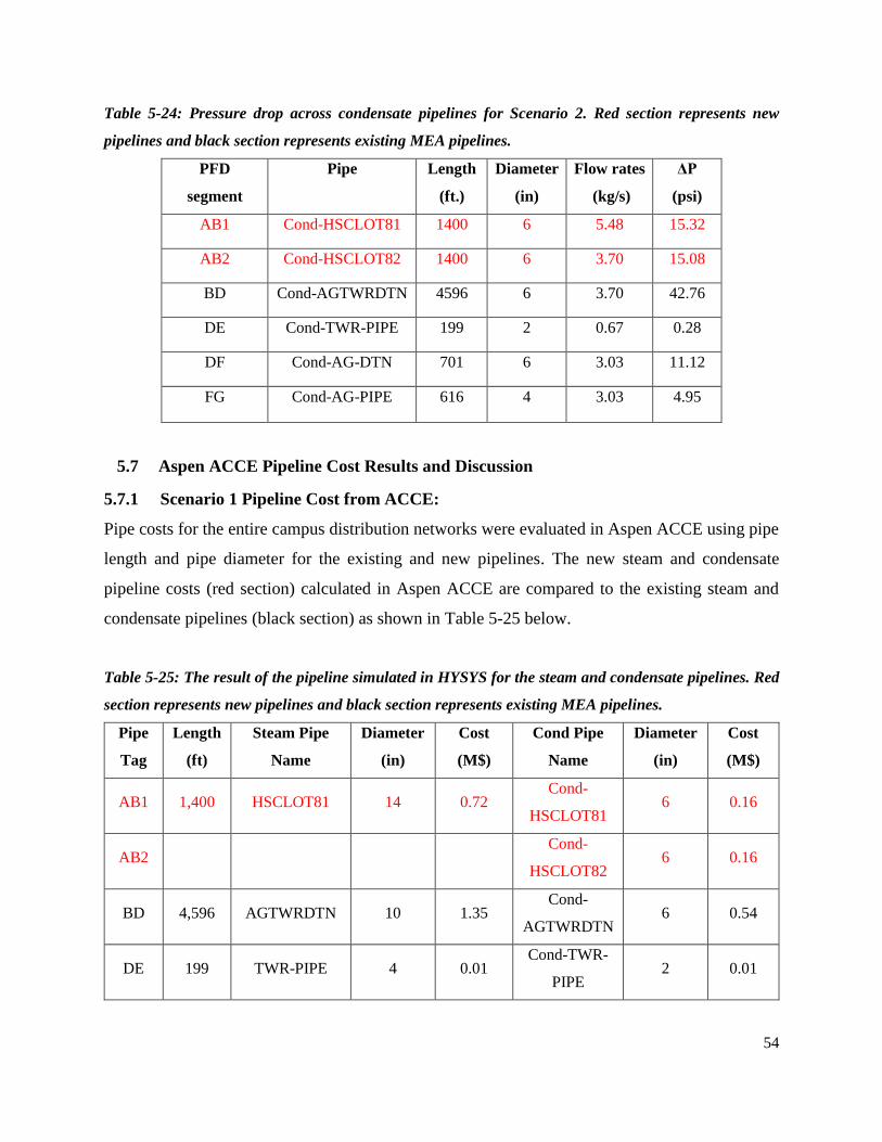
54
Table 5-24: Pressure drop across condensate pipelines for Scenario 2. Red section represents new
pipelines and black section represents existing MEA pipelines.
PFD
segment
Pipe Length
(ft.)
Diameter
(in)
Flow rates
(kg/s)
ΔP
(psi)
AB1 Cond-HSCLOT81 1400 6 5.48 15.32
AB2 Cond-HSCLOT82 1400 6 3.70 15.08
BD Cond-AGTWRDTN 4596 6 3.70 42.76
DE Cond-TWR-PIPE 199 2 0.67 0.28
DF Cond-AG-DTN 701 6 3.03 11.12
FG Cond-AG-PIPE 616 4 3.03 4.95
5.7 Aspen ACCE Pipeline Cost Results and Discussion
5.7.1 Scenario 1 Pipeline Cost from ACCE:
Pipe costs for the entire campus distribution networks were evaluated in Aspen ACCE using pipe
length and pipe diameter for the existing and new pipelines. The new steam and condensate
pipeline costs (red section) calculated in Aspen ACCE are compared to the existing steam and
condensate pipelines (black section) as shown in Table 5-25 below.
Table 5-25: The result of the pipeline simulated in HYSYS for the steam and condensate pipelines. Red
section represents new pipelines and black section represents existing MEA pipelines.
Pipe
Tag
Length
(ft)
Steam Pipe
Name
Diameter
(in)
Cost
(M$)
Cond Pipe
Name
Diameter
(in)
Cost
(M$)
AB1 1,400 HSCLOT81 14 0.72 Cond-
HSCLOT81 6 0.16
AB2 Cond-
HSCLOT82 6 0.16
BD 4,596 AGTWRDTN 10 1.35 Cond-
AGTWRDTN 6 0.54
DE 199 TWR-PIPE 4 0.01 Cond-TWR-
PIPE 2 0.01
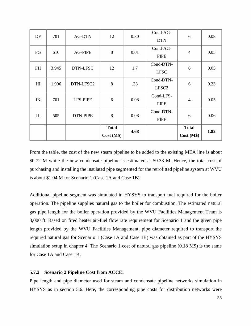
55
DF 701 AG-DTN 12 0.30 Cond-AG-
DTN 6 0.08
FG 616 AG-PIPE 8 0.01 Cond-AG-
PIPE 4 0.05
FH 3,945 DTN-LFSC 12 1.7 Cond-DTN-
LFSC 6 0.05
HI 1,996 DTN-LFSC2 8 .33 Cond-DTN-
LFSC2 6 0.23
JK 701 LFS-PIPE 6 0.08 Cond-LFS-
PIPE 4 0.05
JL 505 DTN-PIPE 8 0.08 Cond-DTN-
PIPE 6 0.06
Total
Cost (M$) 4.68
Total
Cost (M$) 1.82
From the table, the cost of the new steam pipeline to be added to the existing MEA line is about
$0.72 M while the new condensate pipeline is estimated at $0.33 M. Hence, the total cost of
purchasing and installing the insulated pipe segmented for the retrofitted pipeline system at WVU
is about $1.04 M for Scenario 1 (Case 1A and Case 1B).
Additional pipeline segment was simulated in HYSYS to transport fuel required for the boiler
operation. The pipeline supplies natural gas to the boiler for combustion. The estimated natural
gas pipe length for the boiler operation provided by the WVU Facilities Management Team is
3,000 ft. Based on fired heater air-fuel flow rate requirement for Scenario 1 and the given pipe
length provided by the WVU Facilities Management, pipe diameter required to transport the
required natural gas for Scenario 1 (Case 1A and Case 1B) was obtained as part of the HYSYS
simulation setup in chapter 4. The Scenario 1 cost of natural gas pipeline (0.18 M$) is the same
for Case 1A and Case 1B.
5.7.2 Scenario 2 Pipeline Cost from ACCE:
Pipe length and pipe diameter used for steam and condensate pipeline networks simulation in
HYSYS as in section 5.6. Here, the corresponding pipe costs for distribution networks were
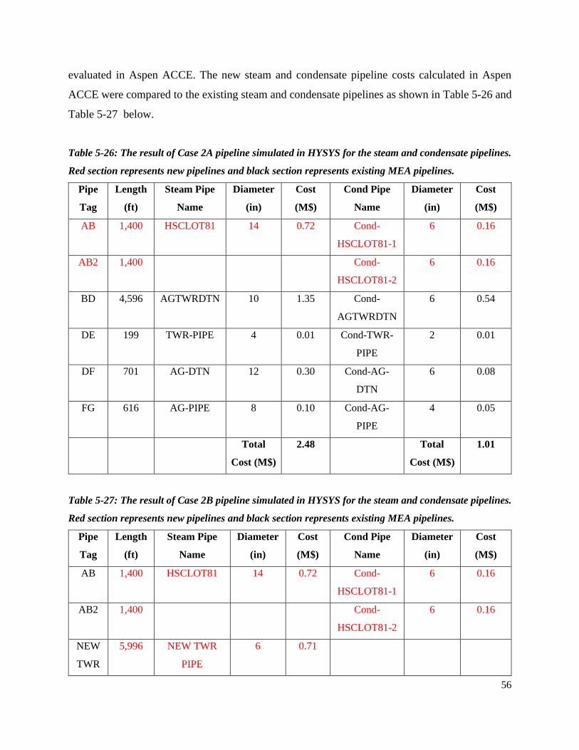
56
evaluated in Aspen ACCE. The new steam and condensate pipeline costs calculated in Aspen
ACCE were compared to the existing steam and condensate pipelines as shown in Table 5-26 and
Table 5-27 below.
Table 5-26: The result of Case 2A pipeline simulated in HYSYS for the steam and condensate pipelines.
Red section represents new pipelines and black section represents existing MEA pipelines.
Pipe
Tag
Length
(ft)
Steam Pipe
Name
Diameter
(in)
Cost
(M$)
Cond Pipe
Name
Diameter
(in)
Cost
(M$)
AB 1,400 HSCLOT81 14 0.72 Cond-
HSCLOT81-1
6 0.16
AB2 1,400
Cond-
HSCLOT81-2
6 0.16
BD 4,596 AGTWRDTN 10 1.35 Cond-
AGTWRDTN
6 0.54
DE 199 TWR-PIPE 4 0.01 Cond-TWR-
PIPE
2 0.01
DF 701 AG-DTN 12 0.30 Cond-AG-
DTN
6 0.08
FG 616 AG-PIPE 8 0.10 Cond-AG-
PIPE
4 0.05
Total
Cost (M$)
2.48
Total
Cost (M$)
1.01
Table 5-27: The result of Case 2B pipeline simulated in HYSYS for the steam and condensate pipelines.
Red section represents new pipelines and black section represents existing MEA pipelines.
Pipe
Tag
Length
(ft)
Steam Pipe
Name
Diameter
(in)
Cost
(M$)
Cond Pipe
Name
Diameter
(in)
Cost
(M$)
AB 1,400 HSCLOT81 14 0.72 Cond-
HSCLOT81-1
6 0.16
AB2 1,400
Cond-
HSCLOT81-2
6 0.16
NEW
TWR
5,996 NEW TWR
PIPE
6 0.71
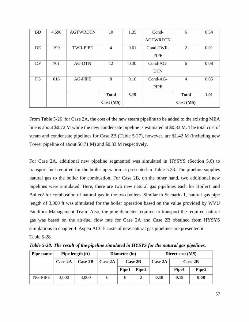
57
BD 4,596 AGTWRDTN 10 1.35 Cond-
AGTWRDTN
6 0.54
DE 199 TWR-PIPE 4 0.01 Cond-TWR-
PIPE
2 0.01
DF 701 AG-DTN 12 0.30 Cond-AG-
DTN
6 0.08
FG 616 AG-PIPE 8 0.10 Cond-AG-
PIPE
4 0.05
Total
Cost (M$)
3.19
Total
Cost (M$)
1.01
From Table 5-26 for Case 2A, the cost of the new steam pipeline to be added to the existing MEA
line is about $0.72 M while the new condensate pipeline is estimated at $0.33 M. The total cost of
steam and condensate pipelines for Case 2B (Table 5-27), however, are $1.42 M (including new
Tower pipeline of about $0.71 M) and $0.33 M respectively.
For Case 2A, additional new pipeline segmented was simulated in HYSYS (Section 5.6) to
transport fuel required for the boiler operation as presented in Table 5.28. The pipeline supplies
natural gas to the boiler for combustion. For Case 2B, on the other hand, two additional new
pipelines were simulated. Here, there are two new natural gas pipelines each for Boiler1 and
Boiler2 for combustion of natural gas in the two boilers. Similar to Scenario 1, natural gas pipe
length of 3,000 ft was simulated for the boiler operation based on the value provided by WVU
Facilities Management Team. Also, the pipe diameter required to transport the required natural
gas was based on the air-fuel flow rate for Case 2A and Case 2B obtained from HYSYS
simulations in chapter 4. Aspen ACCE costs of new natural gas pipelines are presented in
Table 5-28.
Table 5-28: The result of the pipeline simulated in HYSYS for the natural gas pipelines.
Pipe name Pipe length (ft) Diameter (in) Direct cost (M$)
Case 2A Case 2B Case 2A Case 2B Case 2A Case 2B
Pipe1 Pipe2 Pipe1 Pipe2
NG-PIPE 3,000 3,000 6 6 2 0.18 0.18 0.08
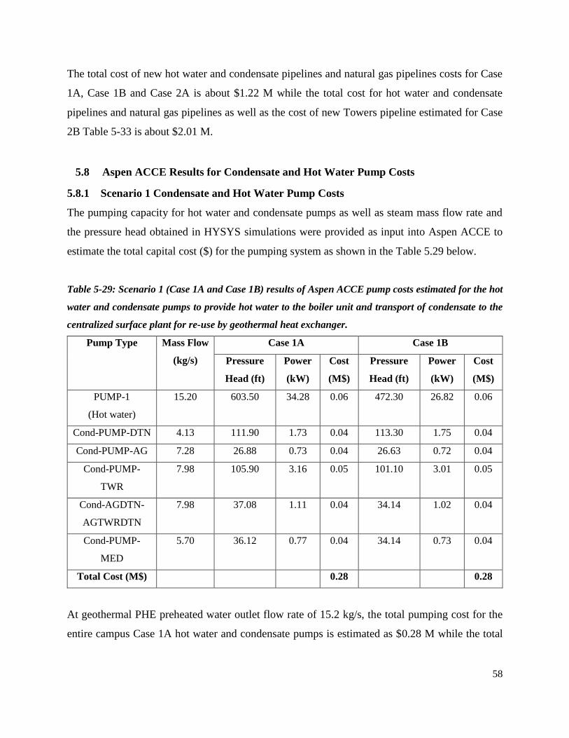
58
The total cost of new hot water and condensate pipelines and natural gas pipelines costs for Case
1A, Case 1B and Case 2A is about $1.22 M while the total cost for hot water and condensate
pipelines and natural gas pipelines as well as the cost of new Towers pipeline estimated for Case
2B Table 5-33 is about $2.01 M.
5.8 Aspen ACCE Results for Condensate and Hot Water Pump Costs
5.8.1 Scenario 1 Condensate and Hot Water Pump Costs
The pumping capacity for hot water and condensate pumps as well as steam mass flow rate and
the pressure head obtained in HYSYS simulations were provided as input into Aspen ACCE to
estimate the total capital cost ($) for the pumping system as shown in the Table 5.29 below.
Table 5-29: Scenario 1 (Case 1A and Case 1B) results of Aspen ACCE pump costs estimated for the hot
water and condensate pumps to provide hot water to the boiler unit and transport of condensate to the
centralized surface plant for re-use by geothermal heat exchanger.
Pump Type Mass Flow
(kg/s)
Case 1A Case 1B
Pressure
Head (ft)
Power
(kW)
Cost
(M$)
Pressure
Head (ft)
Power
(kW)
Cost
(M$)
PUMP-1
(Hot water)
15.20 603.50 34.28 0.06 472.30 26.82 0.06
Cond-PUMP-DTN 4.13 111.90 1.73 0.04 113.30 1.75 0.04
Cond-PUMP-AG 7.28 26.88 0.73 0.04 26.63 0.72 0.04
Cond-PUMP-
TWR
7.98 105.90 3.16 0.05 101.10 3.01 0.05
Cond-AGDTN-
AGTWRDTN
7.98 37.08 1.11 0.04 34.14 1.02 0.04
Cond-PUMP-
MED
5.70 36.12 0.77 0.04 34.14 0.73 0.04
Total Cost (M$)
0.28
0.28
At geothermal PHE preheated water outlet flow rate of 15.2 kg/s, the total pumping cost for the
entire campus Case 1A hot water and condensate pumps is estimated as $0.28 M while the total
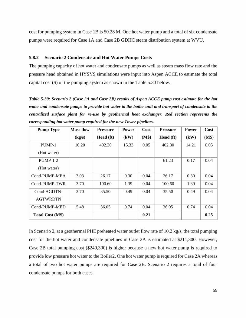
59
cost for pumping system in Case 1B is $0.28 M. One hot water pump and a total of six condensate
pumps were required for Case 1A and Case 2B GDHC steam distribution system at WVU.
5.8.2 Scenario 2 Condensate and Hot Water Pumps Costs
The pumping capacity of hot water and condensate pumps as well as steam mass flow rate and the
pressure head obtained in HYSYS simulations were input into Aspen ACCE to estimate the total
capital cost ($) of the pumping system as shown in the Table 5.30 below.
Table 5-30: Scenario 2 (Case 2A and Case 2B) results of Aspen ACCE pump cost estimate for the hot
water and condensate pumps to provide hot water to the boiler unit and transport of condensate to the
centralized surface plant for re-use by geothermal heat exchanger. Red section represents the
corresponding hot water pump required for the new Tower pipelines.
Pump Type Mass flow
(kg/s)
Pressure
Head (ft)
Power
(kW)
Cost
(M$)
Pressure
Head (ft)
Power
(kW)
Cost
(M$)
PUMP-1
(Hot water)
10.20 402.30 15.33 0.05 402.30 14.21 0.05
PUMP-1-2
(Hot water)
61.23 0.17 0.04
Cond-PUMP-MEA 3.03 26.17 0.30 0.04 26.17 0.30 0.04
Cond-PUMP-TWR 3.70 100.60 1.39 0.04 100.60 1.39 0.04
Cond-AGDTN-
AGTWRDTN
3.70 35.50 0.49 0.04 35.50 0.49 0.04
Cond-PUMP-MED 5.48 36.05 0.74 0.04 36.05 0.74 0.04
Total Cost (M$)
0.21
0.25
In Scenario 2, at a geothermal PHE preheated water outlet flow rate of 10.2 kg/s, the total pumping
cost for the hot water and condensate pipelines in Case 2A is estimated at $211,300. However,
Case 2B total pumping cost ($249,300) is higher because a new hot water pump is required to
provide low pressure hot water to the Boiler2. One hot water pump is required for Case 2A whereas
a total of two hot water pumps are required for Case 2B. Scenario 2 requires a total of four
condensate pumps for both cases.
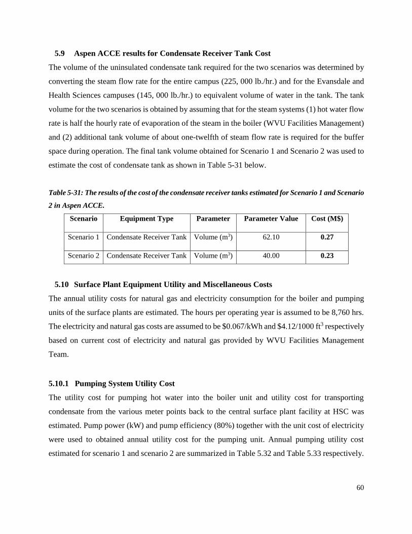
60
5.9 Aspen ACCE results for Condensate Receiver Tank Cost
The volume of the uninsulated condensate tank required for the two scenarios was determined by
converting the steam flow rate for the entire campus (225, 000 lb./hr.) and for the Evansdale and
Health Sciences campuses (145, 000 lb./hr.) to equivalent volume of water in the tank. The tank
volume for the two scenarios is obtained by assuming that for the steam systems (1) hot water flow
rate is half the hourly rate of evaporation of the steam in the boiler (WVU Facilities Management)
and (2) additional tank volume of about one-twelfth of steam flow rate is required for the buffer
space during operation. The final tank volume obtained for Scenario 1 and Scenario 2 was used to
estimate the cost of condensate tank as shown in Table 5-31 below.
Table 5-31: The results of the cost of the condensate receiver tanks estimated for Scenario 1 and Scenario
2 in Aspen ACCE.
Scenario Equipment Type Parameter Parameter Value Cost (M$)
Scenario 1 Condensate Receiver Tank Volume (m3) 62.10 0.27
Scenario 2 Condensate Receiver Tank Volume (m3) 40.00 0.23
5.10 Surface Plant Equipment Utility and Miscellaneous Costs
The annual utility costs for natural gas and electricity consumption for the boiler and pumping
units of the surface plants are estimated. The hours per operating year is assumed to be 8,760 hrs.
The electricity and natural gas costs are assumed to be $0.067/kWh and $4.12/1000 ft3 respectively
based on current cost of electricity and natural gas provided by WVU Facilities Management
Team.
5.10.1 Pumping System Utility Cost
The utility cost for pumping hot water into the boiler unit and utility cost for transporting
condensate from the various meter points back to the central surface plant facility at HSC was
estimated. Pump power (kW) and pump efficiency (80%) together with the unit cost of electricity
were used to obtained annual utility cost for the pumping unit. Annual pumping utility cost
estimated for scenario 1 and scenario 2 are summarized in Table 5.32 and Table 5.33 respectively.
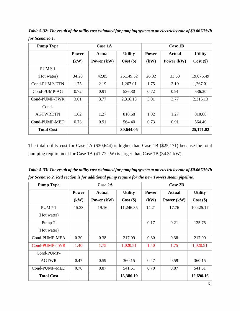
61
Table 5-32: The result of the utility cost estimated for pumping system at an electricity rate of $0.067/kWh
for Scenario 1.
Pump Type Case 1A Case 1B
Power
(kW)
Actual
Power (kW)
Utility
Cost ($)
Power
(kW)
Actual
Power (kW)
Utility
Cost ($)
PUMP-1
(Hot water) 34.28 42.85 25,149.52 26.82 33.53 19,676.49
Cond-PUMP-DTN 1.75 2.19 1,267.01 1.75 2.19 1,267.01
Cond-PUMP-AG 0.72 0.91 536.30 0.72 0.91 536.30
Cond-PUMP-TWR 3.01 3.77 2,316.13 3.01 3.77 2,316.13
Cond-
AGTWRDTN 1.02 1.27 810.68 1.02 1.27 810.68
Cond-PUMP-MED 0.73 0.91 564.40 0.73 0.91 564.40
Total Cost
30,644.05
25,171.02
The total utility cost for Case 1A ($30,644) is higher than Case 1B ($25,171) because the total
pumping requirement for Case 1A (41.77 kW) is larger than Case 1B (34.31 kW).
Table 5-33: The result of the utility cost estimated for pumping system at an electricity rate of $0.067/kWh
for Scenario 2. Red section is for additional pump require for the new Towers steam pipeline.
Pump Type Case 2A Case 2B
Power
(kW)
Actual
Power (kW)
Utility
Cost ($)
Power
(kW)
Actual
Power (kW)
Utility
Cost ($)
PUMP-1
(Hot water)
15.33 19.16 11,246.85 14.21 17.76 10,425.17
Pump-2
(Hot water)
0.17 0.21 125.75
Cond-PUMP-MEA 0.30 0.38 217.09 0.30 0.38 217.09
Cond-PUMP-TWR 1.40 1.75 1,020.51 1.40 1.75 1,020.51
Cond-PUMP-
AGTWR 0.47 0.59 360.15 0.47 0.59 360.15
Cond-PUMP-MED 0.70 0.87 541.51 0.70 0.87 541.51
Total Cost
13,386.10
12,690.16
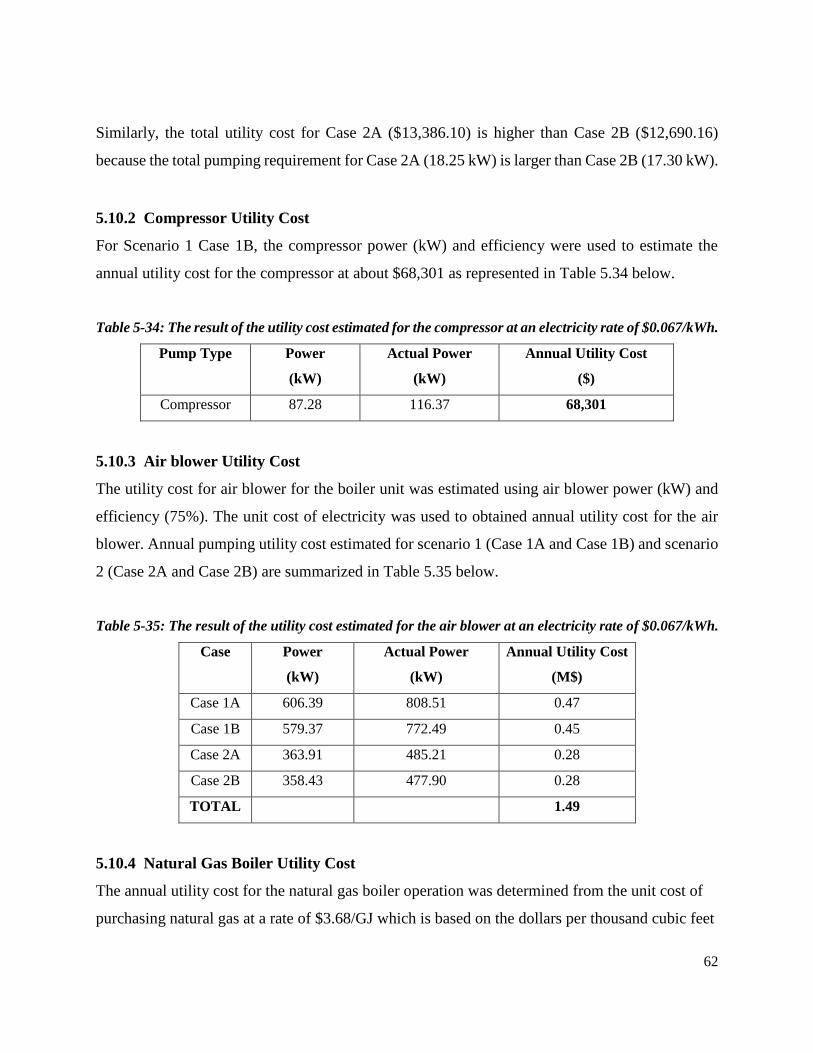
62
Similarly, the total utility cost for Case 2A ($13,386.10) is higher than Case 2B ($12,690.16)
because the total pumping requirement for Case 2A (18.25 kW) is larger than Case 2B (17.30 kW).
5.10.2 Compressor Utility Cost
For Scenario 1 Case 1B, the compressor power (kW) and efficiency were used to estimate the
annual utility cost for the compressor at about $68,301 as represented in Table 5.34 below.
Table 5-34: The result of the utility cost estimated for the compressor at an electricity rate of $0.067/kWh.
Pump Type Power
(kW)
Actual Power
(kW)
Annual Utility Cost
($)
Compressor 87.28 116.37 68,301
5.10.3 Air blower Utility Cost
The utility cost for air blower for the boiler unit was estimated using air blower power (kW) and
efficiency (75%). The unit cost of electricity was used to obtained annual utility cost for the air
blower. Annual pumping utility cost estimated for scenario 1 (Case 1A and Case 1B) and scenario
2 (Case 2A and Case 2B) are summarized in Table 5.35 below.
Table 5-35: The result of the utility cost estimated for the air blower at an electricity rate of $0.067/kWh.
Case Power
(kW)
Actual Power
(kW)
Annual Utility Cost
(M$)
Case 1A 606.39 808.51 0.47
Case 1B 579.37 772.49 0.45
Case 2A 363.91 485.21 0.28
Case 2B 358.43 477.90 0.28
TOTAL
1.49
5.10.4 Natural Gas Boiler Utility Cost
The annual utility cost for the natural gas boiler operation was determined from the unit cost of
purchasing natural gas at a rate of $3.68/GJ which is based on the dollars per thousand cubic feet
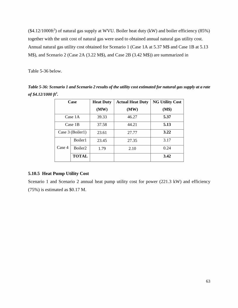
63
($4.12/1000ft3) of natural gas supply at WVU. Boiler heat duty (kW) and boiler efficiency (85%)
together with the unit cost of natural gas were used to obtained annual natural gas utility cost.
Annual natural gas utility cost obtained for Scenario 1 (Case 1A at 5.37 M$ and Case 1B at 5.13
M$), and Scenario 2 (Case 2A (3.22 M$), and Case 2B (3.42 M$)) are summarized in
Table 5-36 below.
Table 5-36: Scenario 1 and Scenario 2 results of the utility cost estimated for natural gas supply at a rate
of $4.12/1000 ft3.
Case Heat Duty
(MW)
Actual Heat Duty
(MW)
NG Utility Cost
(M$)
Case 1A 39.33 46.27 5.37
Case 1B 37.58 44.21 5.13
Case 3 (Boiler1) 23.61 27.77 3.22
Case 4
Boiler1 23.45 27.35 3.17
Boiler2 1.79 2.10 0.24
TOTAL 3.42
5.10.5 Heat Pump Utility Cost
Scenario 1 and Scenario 2 annual heat pump utility cost for power (221.3 kW) and efficiency
(75%) is estimated as $0.17 M.

64
Objective 4: Perform an Economic Analysis to Estimate the Levelized Cost of Heat
(LCOH) Using GEOPHIRES
In this chapter, the total costs of associated major surface plant equipment and distribution
pipelines required for the economic evaluation are summarized. The total surface plant costs
estimated combined with subsurface, surface, and financial parameters were used to run
GEOPHIRES simulations [22]. The LCOH for the proposed hybrid GDHC is determined using
GEOPHIRES software, while the LCOH for the natural gas fired boiler (NGFB) system without
geothermal or heat pump is calculated in Microsoft Excel.
6.1 Economic Evaluation
Following the design of the surface plant for the DHC system at WVU, an economic evaluation of
the proposed hybrid GDHC system was performed in GEOPHIRES. GEOPHIRES is a software
used to perform techno-economic analysis of a geothermal energy system [22], [45], [58]. Here,
the objective is to determine the economic feasibility of the hybrid GDHC system in order to
compare the costs and benefits of the proposed hybrid GDHC system with the existing MEA coal-
fired steam-based system. To achieve this objective, first the LCOH was evaluated in
GEOPHIRES [22], [40], [41], [58], [59]. The parameters used to calculate the levelized cost of
heat (LCOH) include:
• The amount of heat produced over the project lifetime (30 years)
• The capital cost of investment and
• Operating and maintenance costs (O&M)
To calculate LCOH, GEOPHIRES has built-in correlations to estimate the capital cost of
investment and O&M costs [45].
The capital cost of investment (Ccap) is calculated as the sum of:
• Well drilling and completion cost (Cwell)
• Reservoir stimulation costs (Cstim)
• Fluid distribution costs (Cdistr)
• Resource exploration costs (Cexpl)
• Surface plant equipment and distribution costs (Csurf)
65
The sum of these costs (Ccap) are summarized as follows:
𝐶𝑐𝑎𝑝 = 𝐶𝑤𝑒𝑙𝑙 + 𝐶𝑠𝑡𝑖𝑚 + 𝐶𝑑𝑖𝑠𝑡 + 𝐶𝑒𝑥𝑝𝑙 + 𝐶𝑠𝑢𝑟𝑓 (7.1)
However, surface plant cost model available in GEOPHIRES is only suitable for simple cost
calculations as the model is not applicable for detailed estimation of the major components of the
surface plant equipment and distribution pipelines costs (Csurf). As a result, Aspen Plus, Aspen
HYSYS and Aspen exchanger design and rating (EDR) were used in basic surface plant equipment
and distribution network simulations and designs while the costs of various components of the
equipment employed in the surface plant designs were estimated using Aspen economic analyzer
including Aspen capital cost estimator (ACCE). Certain equipment costs including natural gas
boiler and heat pump system, on the other hand, were obtained from the vendors.
Similarly, the annual plant operating and maintenance costs (CO&M, plant) are calculated as the sum
of:
• Surface plant O&M costs (CO&M, surf)
• Wellfield O&M costs (CO&M, well)
• Make-up water costs (CO&M, water)
• Surface plant utilities and natural gas costs (CU&NG, surf)
The sum of these costs (CO&M, plant) are summarized as follows:
𝐶𝑝𝑙𝑎𝑛𝑡 = 𝐶𝑂&𝑀,𝑠𝑢𝑟𝑓 + 𝐶𝑂&𝑀,𝑤𝑒𝑙𝑙 + 𝐶𝑂&𝑀,𝑤𝑎𝑡𝑒𝑟 + 𝐶𝑈&𝑁𝐺,𝑠𝑢𝑟𝑓 (7.2)
However, the rate of water loss in the geothermal reservoir is assumed to be negligible. As a result,
the annual expenses for the make-up water is assumed to be zero for the GDHC system at WVU.
6.1.1 Editing GEOPHIRES
In this work, the hybrid geothermal-natural gas boiler district heating and cooling system was
designed for the WVU. GEOPHIRES V2.0 python code [45], however, can only simulate and
calculate LCOH for the geothermal system. Consequently, GEOPHIRES code was edited to
account for the hybrid system in the LCOH calculation. GEOPHIRES code was modified for the
hybrid system to include the following parameters in LCOH calculation:
66
• Boiler heating duty
• Natural gas utility cost
The boiler heat duty is obtained from Aspen simulators. The total annual natural gas utility cost is
calculated based on the annual fuel flow rate required for steam production by the boiler. The
utility costs for the pump, compressor and air blower are calculated using the average electricity
rate for the WVU campus ($0.067/kWh).
6.1.2 Levelized Cost of Heat (LCOH) Model
Currently, there are three economic models available in GEOPHIRES to calculate LCOH. These
models are:
1. Fixed charge rate (FCR) model
2. Standard levelized cost (SLC) model
3. BICYCLE levelized life cycle cost model
However, BICYCLE levelized cost model is the most robust model [60]. The BICYCLE model
was used to evaluate feasibility of GDHC system at WVU because it is the most complex and the
most realistic economic model which accounts for inflation rate, tax rates and tax credits. The
model assumes the GDHC system at WVU is financed through debt (bonds) and equity and allows
variation of the ratio of these two variables to model LCOH [59]. The LCOH expressed in
$/MMBTU is calculated as follows:
𝐿𝐶𝑂𝐻 = 𝑁𝑃𝑉
∑𝑊𝑡 𝑥 (1 + 𝑖𝑖𝑛𝑓)𝑡
(1 + 𝑖′)𝑡𝑛𝑡=1
(7.4)
where NPV is the net present value, iinf is the inflation rate, 𝑖′ is the average return on investment
and Wt is the nominal thermal output in kWth, and n is the plant life (30 years).
6.2 Levelized Cost of Heat (LCOH) Calculations
Levelized cost of heat estimates here are primarily based on the existing district heating and
cooling system at WVU and may have ignored other important features that may be specific to
67
other locations. LCOH may depend significantly on other factors such as drilling costs, geothermal
gradient, operating hours or energy utilization factor, flow rate per well, surface plant O&M costs,
plant lifetime, discount rates, economic risk and regional considerations including existing
infrastructure. Furthermore, no subsidies, tax incentives, CO2 credits were included in the LCOH
calculations. For comparison purposes, LCOH comparisons should take these factors into
consideration as geothermal resource is geographically localized.
6.3 Total Surface Plant and Capital Cost for Scenario 1 and Scenario 2.
As stated in section 6.1, there is no built-in correlations in GEOPHIRES to calculate surface plant
cost. Thus, costs of the major surface plant equipment for Scenario 1 (Case 1A and Case 1B and
Scenario 2 (Case 2A and Case 2B) were obtained in Aspen ACCE. The direct costs of purchasing
geothermal surface plant equipment including plate heat exchanger, fuel preheater, hot water and
condensate pumps, condensate receiver tank as well as the costs of retrofitted pipelines obtained
in Aspen ACCE are summarized in Table 6-1. In addition, as well as the vendor’s quotes for the
boiler and heat pump system are also presented in Table 6-1. Indirect costs including construction
expense, contingency, contractor fees and engineering expenses are assumed to be 35% of the total
direct and indirect costs [57], [61]. Hence, the total surface plant indirect costs for Scenario 1 and
Scenario 2 are obtained as 54% of the total direct costs. The sum of direct and indirect costs is the
fixed capital investment [57]. The fixed capital investment is equivalent to total module costs [62].
Total capital investment is made up of fixed capital investment and working capital. Working
capital is the additional cost, apart from fixed capital investment, to startup the project and keep
the surface plant in operation. The working capital necessary for the hybrid surface plant operation
is assumed to be 20% of the total capital investment for the project [57]. Scenario 1 and Scenario
2 working capital is calculated as 25% of the fixed capital investment (total direct and indirect
costs). The utility costs for the pumping system, compressor, natural gas and air blower and the
total capital costs for the surface plant facilities make up the total project costs summarized in
Table 6-1. The annual O&M costs for the surface plant equipment is estimated to be 20% of the
total surface plant cost and they are assumed to scale with the size of the surface equipment.
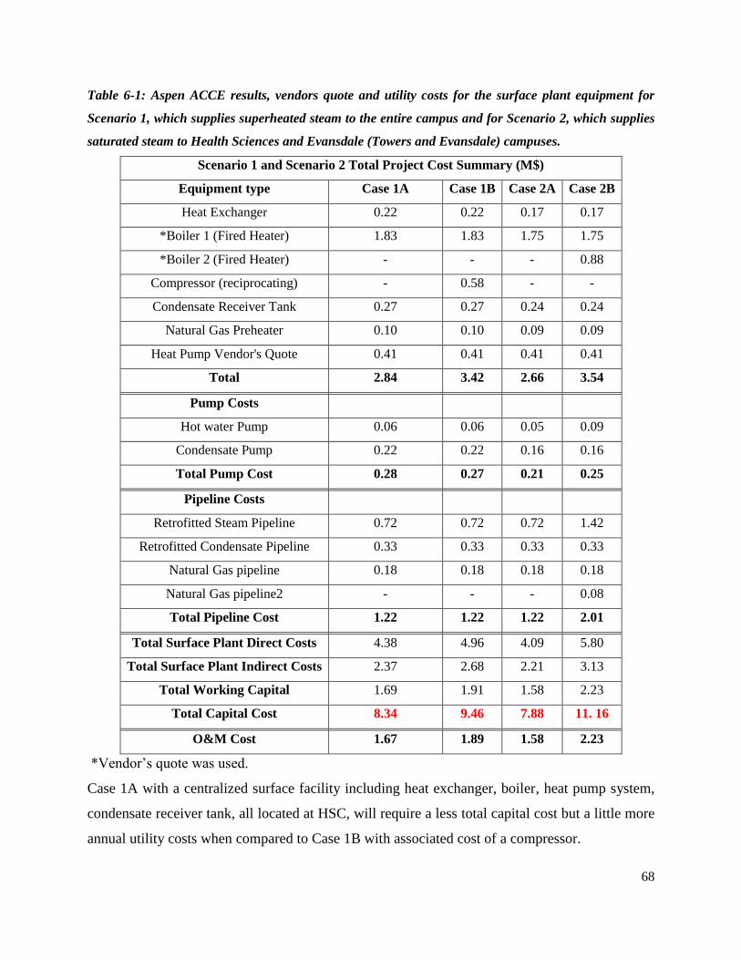
68
Table 6-1: Aspen ACCE results, vendors quote and utility costs for the surface plant equipment for
Scenario 1, which supplies superheated steam to the entire campus and for Scenario 2, which supplies
saturated steam to Health Sciences and Evansdale (Towers and Evansdale) campuses.
Scenario 1 and Scenario 2 Total Project Cost Summary (M$)
Equipment type Case 1A Case 1B Case 2A Case 2B
Heat Exchanger 0.22 0.22 0.17 0.17
*Boiler 1 (Fired Heater) 1.83 1.83 1.75 1.75
*Boiler 2 (Fired Heater) - - - 0.88
Compressor (reciprocating) - 0.58 - -
Condensate Receiver Tank 0.27 0.27 0.24 0.24
Natural Gas Preheater 0.10 0.10 0.09 0.09
Heat Pump Vendor's Quote 0.41 0.41 0.41 0.41
Total 2.84 3.42 2.66 3.54
Pump Costs
Hot water Pump 0.06 0.06 0.05 0.09
Condensate Pump 0.22 0.22 0.16 0.16
Total Pump Cost 0.28 0.27 0.21 0.25
Pipeline Costs
Retrofitted Steam Pipeline 0.72 0.72 0.72 1.42
Retrofitted Condensate Pipeline 0.33 0.33 0.33 0.33
Natural Gas pipeline 0.18 0.18 0.18 0.18
Natural Gas pipeline2 - - - 0.08
Total Pipeline Cost 1.22 1.22 1.22 2.01
Total Surface Plant Direct Costs 4.38 4.96 4.09 5.80
Total Surface Plant Indirect Costs 2.37 2.68 2.21 3.13
Total Working Capital 1.69 1.91 1.58 2.23
Total Capital Cost 8.34 9.46 7.88 11. 16
O&M Cost 1.67 1.89 1.58 2.23
*Vendor’s quote was used.
Case 1A with a centralized surface facility including heat exchanger, boiler, heat pump system,
condensate receiver tank, all located at HSC, will require a less total capital cost but a little more
annual utility costs when compared to Case 1B with associated cost of a compressor.
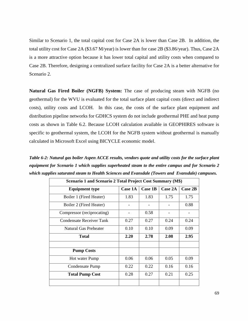
69
Similar to Scenario 1, the total capital cost for Case 2A is lower than Case 2B. In addition, the
total utility cost for Case 2A ($3.67 M/year) is lower than for case 2B ($3.86/year). Thus, Case 2A
is a more attractive option because it has lower total capital and utility costs when compared to
Case 2B. Therefore, designing a centralized surface facility for Case 2A is a better alternative for
Scenario 2.
Natural Gas Fired Boiler (NGFB) System: The case of producing steam with NGFB (no
geothermal) for the WVU is evaluated for the total surface plant capital costs (direct and indirect
costs), utility costs and LCOH. In this case, the costs of the surface plant equipment and
distribution pipeline networks for GDHCS system do not include geothermal PHE and heat pump
costs as shown in Table 6.2. Because LCOH calculation available in GEOPHIRES software is
specific to geothermal system, the LCOH for the NGFB system without geothermal is manually
calculated in Microsoft Excel using BICYCLE economic model.
Table 6-2: Natural gas boiler Aspen ACCE results, vendors quote and utility costs for the surface plant
equipment for Scenario 1 which supplies superheated steam to the entire campus and for Scenario 2
which supplies saturated steam to Health Sciences and Evansdale (Towers and Evansdale) campuses.
Scenario 1 and Scenario 2 Total Project Cost Summary (M$)
Equipment type Case 1A Case 1B Case 2A Case 2B
Boiler 1 (Fired Heater) 1.83 1.83 1.75 1.75
Boiler 2 (Fired Heater) - - - 0.88
Compressor (reciprocating) - 0.58 - -
Condensate Receiver Tank 0.27 0.27 0.24 0.24
Natural Gas Preheater 0.10 0.10 0.09 0.09
Total 2.20 2.78 2.08 2.95
Pump Costs
Hot water Pump 0.06 0.06 0.05 0.09
Condensate Pump 0.22 0.22 0.16 0.16
Total Pump Cost 0.28 0.27 0.21 0.25
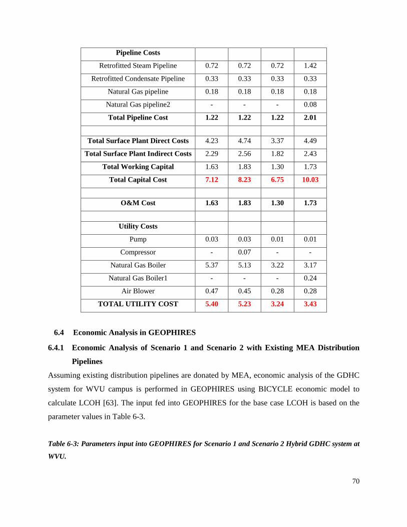
70
Pipeline Costs
Retrofitted Steam Pipeline 0.72 0.72 0.72 1.42
Retrofitted Condensate Pipeline 0.33 0.33 0.33 0.33
Natural Gas pipeline 0.18 0.18 0.18 0.18
Natural Gas pipeline2 - - - 0.08
Total Pipeline Cost 1.22 1.22 1.22 2.01
Total Surface Plant Direct Costs 4.23 4.74 3.37 4.49
Total Surface Plant Indirect Costs 2.29 2.56 1.82 2.43
Total Working Capital 1.63 1.83 1.30 1.73
Total Capital Cost 7.12 8.23 6.75 10.03
O&M Cost 1.63 1.83 1.30 1.73
Utility Costs
Pump 0.03 0.03 0.01 0.01
Compressor - 0.07 - -
Natural Gas Boiler 5.37 5.13 3.22 3.17
Natural Gas Boiler1 - - - 0.24
Air Blower 0.47 0.45 0.28 0.28
TOTAL UTILITY COST 5.40 5.23 3.24 3.43
6.4 Economic Analysis in GEOPHIRES
6.4.1 Economic Analysis of Scenario 1 and Scenario 2 with Existing MEA Distribution
Pipelines
Assuming existing distribution pipelines are donated by MEA, economic analysis of the GDHC
system for WVU campus is performed in GEOPHIRES using BICYCLE economic model to
calculate LCOH [63]. The input fed into GEOPHIRES for the base case LCOH is based on the
parameter values in Table 6-3.
Table 6-3: Parameters input into GEOPHIRES for Scenario 1 and Scenario 2 Hybrid GDHC system at
WVU.
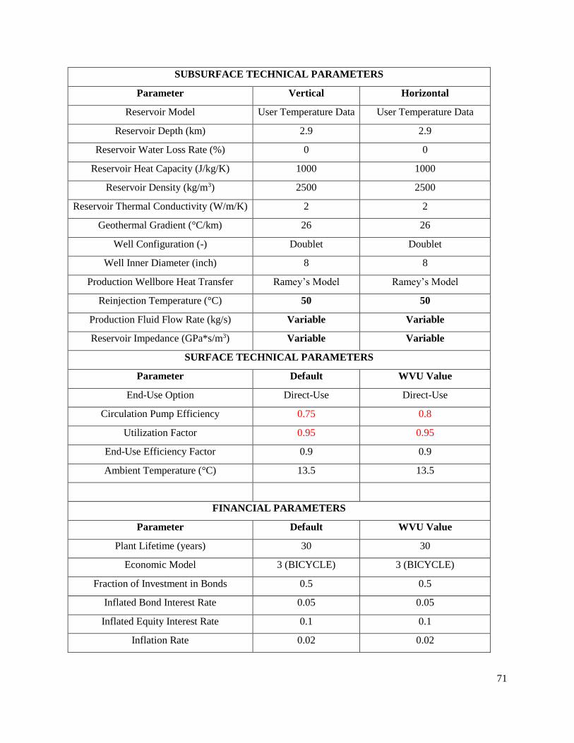
71
SUBSURFACE TECHNICAL PARAMETERS
Parameter Vertical Horizontal
Reservoir Model User Temperature Data User Temperature Data
Reservoir Depth (km) 2.9 2.9
Reservoir Water Loss Rate (%) 0 0
Reservoir Heat Capacity (J/kg/K) 1000 1000
Reservoir Density (kg/m3) 2500 2500
Reservoir Thermal Conductivity (W/m/K) 2 2
Geothermal Gradient (°C/km) 26 26
Well Configuration (-) Doublet Doublet
Well Inner Diameter (inch) 8 8
Production Wellbore Heat Transfer Ramey’s Model Ramey’s Model
Reinjection Temperature (°C) 50 50
Production Fluid Flow Rate (kg/s) Variable Variable
Reservoir Impedance (GPa*s/m3) Variable Variable
SURFACE TECHNICAL PARAMETERS
Parameter Default WVU Value
End-Use Option Direct-Use Direct-Use
Circulation Pump Efficiency 0.75 0.8
Utilization Factor 0.95 0.95
End-Use Efficiency Factor 0.9 0.9
Ambient Temperature (°C) 13.5 13.5
FINANCIAL PARAMETERS
Parameter Default WVU Value
Plant Lifetime (years) 30 30
Economic Model 3 (BICYCLE) 3 (BICYCLE)
Fraction of Investment in Bonds 0.5 0.5
Inflated Bond Interest Rate 0.05 0.05
Inflated Equity Interest Rate 0.1 0.1
Inflation Rate 0.02 0.02
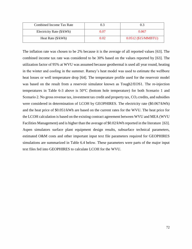
72
Combined Income Tax Rate 0.3 0.3
Electricity Rate ($/kWh) 0.07 0.067
Heat Rate ($/kWh) 0.02 0.0512 ($15/MMBTU)
The inflation rate was chosen to be 2% because it is the average of all reported values [63]. The
combined income tax rate was considered to be 30% based on the values reported by [63]. The
utilization factor of 95% at WVU was assumed because geothermal is used all year round, heating
in the winter and cooling in the summer. Ramey’s heat model was used to estimate the wellbore
heat losses or well temperature drop [64]. The temperature profile used for the reservoir model
was based on the result from a reservoir simulator known as Tough2/EOS1. The re-injection
temperatures in Table 6-3 above is 50°C (bottom hole temperature) for both Scenario 1 and
Scenario 2. No gross revenue tax, investment tax credit and property tax, CO2 credits, and subsidies
were considered in determination of LCOH by GEOPHIRES. The electricity rate ($0.067/kWh)
and the heat price of $0.051/kWh are based on the current rates for the WVU. The heat price for
the LCOH calculation is based on the existing contract agreement between WVU and MEA (WVU
Facilities Management) and is higher than the average of $0.02/kWh reported in the literature [63].
Aspen simulators surface plant equipment design results, subsurface technical parameters,
estimated O&M costs and other important input text file parameters required for GEOPHIRES
simulations are summarized in Table 6.4 below. These parameters were parts of the major input
text files fed into GEOPHIRES to calculate LCOH for the WVU.
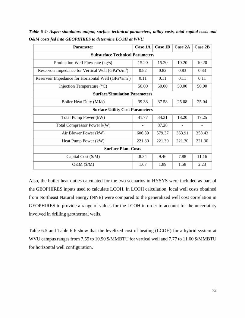
73
Table 6-4: Aspen simulators output, surface technical parameters, utility costs, total capital costs and
O&M costs fed into GEOPHIRES to determine LCOH at WVU.
Parameter Case 1A Case 1B Case 2A Case 2B
Subsurface Technical Parameters
Production Well Flow rate (kg/s) 15.20 15.20 10.20 10.20
Reservoir Impedance for Vertical Well (GPa*s/m3) 0.82 0.82 0.83 0.83
Reservoir Impedance for Horizontal Well (GPa*s/m3) 0.11 0.11 0.11 0.11
Injection Temperature (°C) 50.00 50.00 50.00 50.00
Surface/Simulation Parameters
Boiler Heat Duty (MJ/s) 39.33 37.58 25.08 25.04
Surface Utility Cost Parameters
Total Pump Power (kW) 41.77 34.31 18.20 17.25
Total Compressor Power k(W) - 87.28 - -
Air Blower Power (kW) 606.39 579.37 363.91 358.43
Heat Pump Power (kW) 221.30 221.30 221.30 221.30
Surface Plant Costs
Capital Cost ($/M) 8.34 9.46 7.88 11.16
O&M ($/M) 1.67 1.89 1.58 2.23
Also, the boiler heat duties calculated for the two scenarios in HYSYS were included as part of
the GEOPHIRES inputs used to calculate LCOH. In LCOH calculation, local well costs obtained
from Northeast Natural energy (NNE) were compared to the generalized well cost correlation in
GEOPHIRES to provide a range of values for the LCOH in order to account for the uncertainty
involved in drilling geothermal wells.
Table 6.5 and Table 6-6 show that the levelized cost of heating (LCOH) for a hybrid system at
WVU campus ranges from 7.55 to 10.90 $/MMBTU for vertical well and 7.77 to 11.60 $/MMBTU
for horizontal well configuration.
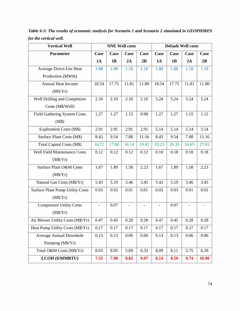
74
Table 6-5: The results of economic analysis for Scenario 1 and Scenario 2 simulated in GEOPHIRES
for the vertical well.
Vertical Well NNE Well costs Default Well costs
Parameter Case
1A
Case
1B
Case
2A
Case
2B
Case
1A
Case
1B
Case
2A
Case
2B
Average Direct-Use Heat
Production (MWth)
1.88 1.88 1.18 1.18 1.88 1.88 1.18 1.18
Annual Heat Income
(MS/Yr)
18.54 17.75 11.81 11.80 18.54 17.75 11.81 11.80
Well Drilling and Completion
Costs (M$/Well)
2.10 2.10 2.10 2.10 5.24 5.24 5.24 5.24
Field Gathering System Costs
(M$)
1.27 1.27 1.15 0.98 1.27 1.27 1.15 1.15
Exploration Costs (M$) 2.91 2.91 2.91 2.91 5.14 5.14 5.14 5.14
Surface Plant Costs (M$) 8.43 9.54 7.88 11.16 8.43 9.54 7.88 11.16
Total Capital Costs (M$) 16.72 17.84 16.14 19.42 25.23 26.35 24.65 27.93
Well Field Maintenance Costs
(M$/Yr)
0.12 0.12 0.12 0.12 0.18 0.18 0.18 0.18
Surface Plant O&M Costs
(M$/Yr)
1.67 1.89 1.58 2.23 1.67 1.89 1.58 2.23
Natural Gas Costs (M$/Yr) 5.43 5.19 3.46 3.45 5.43 5.19 3.46 3.45
Surface Plant Pump Utility Costs
(M$/Yr)
0.03 0.03 0.01 0.01 0.03 0.03 0.01 0.01
Compressor Utility Costs
(M$/Yr)
- 0.07 - - - 0.07 - -
Air Blower Utility Costs (M$/Yr) 0.47 0.45 0.28 0.28 0.47 0.45 0.28 0.28
Heat Pump Utility Costs (M$/Yr) 0.17 0.17 0.17 0.17 0.17 0.17 0.17 0.17
Average Annual Downhole
Pumping (M$/Yr)
0.13 0.13 0.06 0.06 0.13 0.13 0.06 0.06
Total O&M Costs (M$/Yr) 8.03 8.05 5.69 6.33 8.09 8.11 5.75 6.39
LCOH ($/MMBTU) 7.55 7.98 8.82 9.97 8.14 8.59 9.74 10.90

75
Table 6-6: The results of economic analysis for Scenario 1 and Scenario 2 simulated in GEOPHIRES
for the horizontal well.
Horizontal Well NNE Well costs Default Well costs
Parameter Case
1A
Case
1B
Case
2A
Case
2B
Case
1A
Case
1B
Case
2A
Case
2B
Average Direct-Use Heat
Production (MWth)
1.85 1.85 1.17 1.17 1.85 1.85 1.17 1.17
Annual Heat Income
(MS/Yr)
18.53 17.74 11.81 11.79 18.53 17.74 11.81 11.79
Well Drilling and Completion
Costs (M$/Well)
3.80 3.80 3.80 3.80 7.86 7.86 7.86 7.86
Field Gathering System Costs
(M$)
1.04 1.04 1.01 1.01 1.04 1.04 1.01 1.01
Exploration Costs (M$) 4.22 4.22 4.22 4.22 7.07 7.07 7.07 7.07
Surface Plant Costs (M$) 8.34 9.46 7.88 11.16 8.34 9.46 7.88 11.16
Total Capital Costs (M$) 21.21 22.33 20.71 23.99 32.17 33.29 31.67 34.95
Well Field Maintenance Costs
(M$/Yr)
0.15 0.15 0.15 0.15 0.23 0.23 0.23 0.23
Surface Plant O&M Costs
(M$/Yr)
1.67 1.89 1.58 2.23 1.67 1.89 1.58 2.23
Natural Gas Costs (M$/Yr) 5.43 5.19 3.46 3.45 5.43 5.19 3.46 3.45
Surface Plant Pump Utility Costs
(M$/Yr)
0.03 0.03 0.01 0.01 0.03 0.03 0.01 0.01
Compressor Utility Costs
(M$/Yr)
- 0.07 - - - 0.07 - -
Air Blower Utility Costs (M$/Yr) 0.47 0.45 0.28 0.28 0.47 0.45 0.28 0.28
Heat Pump Utility Costs (M$/Yr) 0.17 0.17 0.17 0.17 0.17 0.17 0.17 0.17
Average Annual Downhole
Pumping (M$/Yr)
0.01 0.01 0.01 0.01 0.01 0.01 0.01 0.01
Total O&M Costs (M$/Yr) 7.94 7.96 5.67 6.31 8.02 8.04 5.75 6.39
LCOH ($/MMBTU) 7.77 8.21 9.25 10.41 8.53 9.00 10.44 11.60
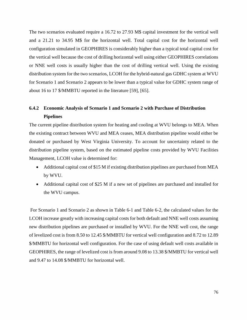
76
The two scenarios evaluated require a 16.72 to 27.93 M$ capital investment for the vertical well
and a 21.21 to 34.95 M$ for the horizontal well. Total capital cost for the horizontal well
configuration simulated in GEOPHIRES is considerably higher than a typical total capital cost for
the vertical well because the cost of drilling horizontal well using either GEOPHIRES correlations
or NNE well costs is usually higher than the cost of drilling vertical well. Using the existing
distribution system for the two scenarios, LCOH for the hybrid-natural gas GDHC system at WVU
for Scenario 1 and Scenario 2 appears to be lower than a typical value for GDHC system range of
about 16 to 17 $/MMBTU reported in the literature [59], [65].
6.4.2 Economic Analysis of Scenario 1 and Scenario 2 with Purchase of Distribution
Pipelines
The current pipeline distribution system for heating and cooling at WVU belongs to MEA. When
the existing contract between WVU and MEA ceases, MEA distribution pipeline would either be
donated or purchased by West Virginia University. To account for uncertainty related to the
distribution pipeline system, based on the estimated pipeline costs provided by WVU Facilities
Management, LCOH value is determined for:
• Additional capital cost of $15 M if existing distribution pipelines are purchased from MEA
by WVU.
• Additional capital cost of $25 M if a new set of pipelines are purchased and installed for
the WVU campus.
For Scenario 1 and Scenario 2 as shown in Table 6-1 and Table 6-2, the calculated values for the
LCOH increase greatly with increasing capital costs for both default and NNE well costs assuming
new distribution pipelines are purchased or installed by WVU. For the NNE well cost, the range
of levelized cost is from 8.50 to 12.45 $/MMBTU for vertical well configuration and 8.72 to 12.89
$/MMBTU for horizontal well configuration. For the case of using default well costs available in
GEOPHIRES, the range of levelized cost is from around 9.08 to 13.38 $/MMBTU for vertical well
and 9.47 to 14.08 $/MMBTU for horizontal well.
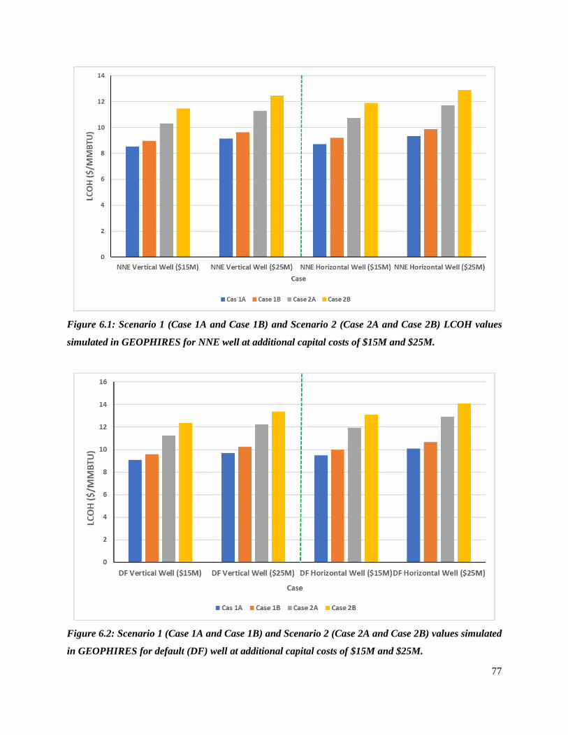
77
Figure 6.1: Scenario 1 (Case 1A and Case 1B) and Scenario 2 (Case 2A and Case 2B) LCOH values
simulated in GEOPHIRES for NNE well at additional capital costs of $15M and $25M.
Figure 6.2: Scenario 1 (Case 1A and Case 1B) and Scenario 2 (Case 2A and Case 2B) values simulated
in GEOPHIRES for default (DF) well at additional capital costs of $15M and $25M.
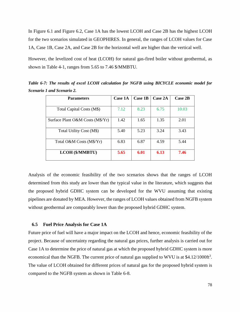
78
In Figure 6.1 and Figure 6.2, Case 1A has the lowest LCOH and Case 2B has the highest LCOH
for the two scenarios simulated in GEOPHIRES. In general, the ranges of LCOH values for Case
1A, Case 1B, Case 2A, and Case 2B for the horizontal well are higher than the vertical well.
However, the levelized cost of heat (LCOH) for natural gas-fired boiler without geothermal, as
shown in Table 4-1, ranges from 5.65 to 7.46 $/MMBTU.
Table 6-7: The results of excel LCOH calculation for NGFB using BICYCLE economic model for
Scenario 1 and Scenario 2.
Parameters Case 1A Case 1B Case 2A Case 2B
Total Capital Costs (M$) 7.12 8.23 6.75 10.03
Surface Plant O&M Costs (M$/Yr) 1.42 1.65 1.35 2.01
Total Utility Cost (M$) 5.40 5.23 3.24 3.43
Total O&M Costs (M$/Yr) 6.83 6.87 4.59 5.44
LCOH ($/MMBTU) 5.65 6.01 6.13 7.46
Analysis of the economic feasibility of the two scenarios shows that the ranges of LCOH
determined from this study are lower than the typical value in the literature, which suggests that
the proposed hybrid GDHC system can be developed for the WVU assuming that existing
pipelines are donated by MEA. However, the ranges of LCOH values obtained from NGFB system
without geothermal are comparably lower than the proposed hybrid GDHC system.
6.5 Fuel Price Analysis for Case 1A
Future price of fuel will have a major impact on the LCOH and hence, economic feasibility of the
project. Because of uncertainty regarding the natural gas prices, further analysis is carried out for
Case 1A to determine the price of natural gas at which the proposed hybrid GDHC system is more
economical than the NGFB. The current price of natural gas supplied to WVU is at $4.12/1000ft3.
The value of LCOH obtained for different prices of natural gas for the proposed hybrid system is
compared to the NGFB system as shown in Table 6-8.
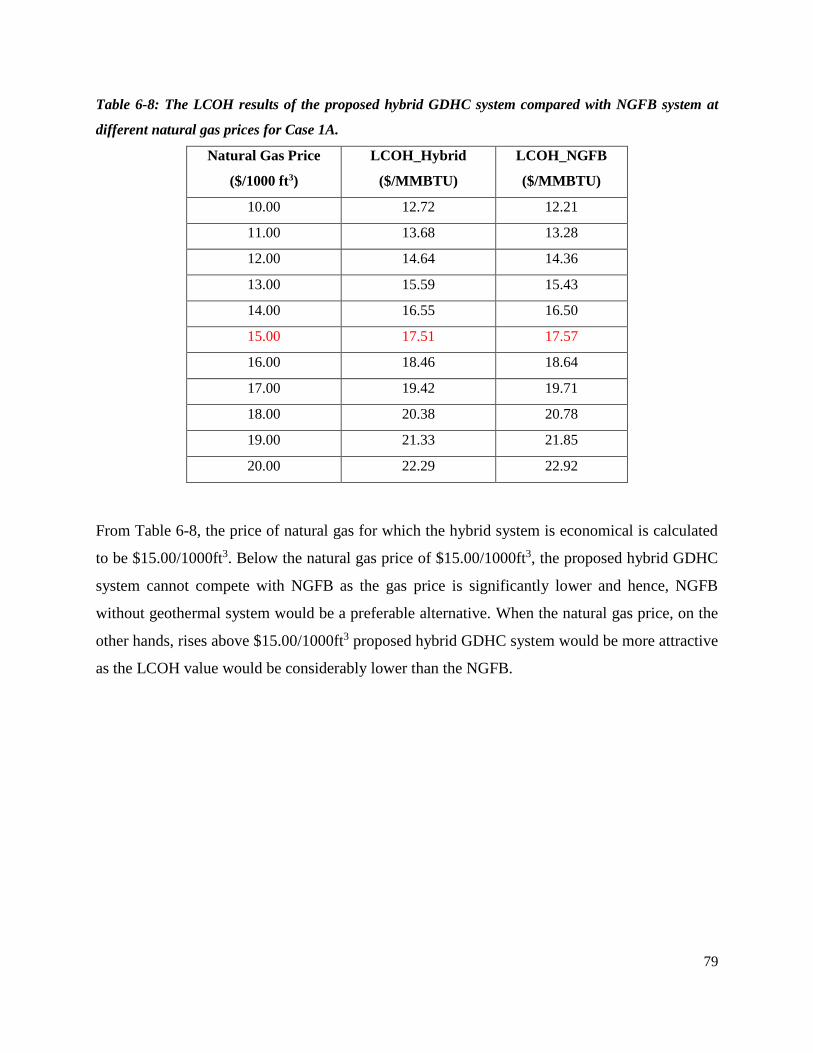
79
Table 6-8: The LCOH results of the proposed hybrid GDHC system compared with NGFB system at
different natural gas prices for Case 1A.
Natural Gas Price
($/1000 ft3)
LCOH_Hybrid
($/MMBTU)
LCOH_NGFB
($/MMBTU)
10.00 12.72 12.21
11.00 13.68 13.28
12.00 14.64 14.36
13.00 15.59 15.43
14.00 16.55 16.50
15.00 17.51 17.57
16.00 18.46 18.64
17.00 19.42 19.71
18.00 20.38 20.78
19.00 21.33 21.85
20.00 22.29 22.92
From Table 6-8, the price of natural gas for which the hybrid system is economical is calculated
to be $15.00/1000ft3. Below the natural gas price of $15.00/1000ft3, the proposed hybrid GDHC
system cannot compete with NGFB as the gas price is significantly lower and hence, NGFB
without geothermal system would be a preferable alternative. When the natural gas price, on the
other hands, rises above $15.00/1000ft3 proposed hybrid GDHC system would be more attractive
as the LCOH value would be considerably lower than the NGFB.

80
Conclusions and Recommendations for the Future Work
7.1 Conclusions
In addition to an elevated temperature hot spot found beneath the Tuscarora Sandstone in
Morgantown, WVU campus has a potential of using geothermal year-round because there is a
relatively large student population (over 30,000) with a dense arrangement of about 245 campus
buildings on 1,892 acres. Thus, WVU’s Morgantown campus has been identified as a prime
location in the eastern United States for the development of a geothermal direct-use heating and
cooling system application.
The main goal of this project was to perform a feasibility analysis of developing a GDHC system
for the WVU campus in Morgantown. First, this work evaluated the current DHC system at West
Virginia University and proposed the use of existing DHC system together with the geothermal
system to supply steam to various campuses. Because the expected geofluid from the well cannot
meet the campus steam demand at temperatures below 100°C, the potential of using low-
temperature geothermal energy with a natural gas boiler was assessed. Aspen simulators were used
to design the proposed geothermal surface plant for the GDHC system at WVU. Natural gas-fired
boiler was integrated with the geothermal system and hence, a hybrid GDHC system was designed.
The resulting hybrid geothermal-natural gas district heating and cooling system was proposed to
replace the existing MEA coal-fired steam-based system.
Because geothermal contribution to the proposed heating and cooling system was very low, this
study further focused on improving the hybrid GDHC system design with the heat pump system.
The heat pump system improvement for the hybrid GDHC system was achieved by further
preheating secondary fluid temperature from 75°C to 90°C and the improved hybrid system
performance was boosted by maximizing geothermal energy utilization in order to minimize the
levelized cost of heat (LCOH). Thus, an integrated hybrid GDHC system with higher efficiency
was achieved using a heat pump. For all scenarios considered in this work, geothermal contributes
between 2.30 to 2.43% to the heating and cooling system at WVU while the improved hybrid
GDHC system with a heat pump contributes between 4.05 to 4.39%.
81
The total capital costs for the two scenarios were determined in Aspen ACCE. Surface plant
equipment and distribution costs for the four cases provided the input required to calculate LCOH
in GEOPHIRES. After obtaining the surface plant capital costs, the BICYCLE model was used to
calculate the LCOH at WVU. The feasibility of the GDHC system was determined by comparing
costs of the proposed hybrid GDHC system with the existing MEA coal-fired steam-based system.
Currently, WVU pays $15/MMBTU for steam supplies by MEA. The preliminary assessment from
the previous work by Nandanwar et. al. [66] calculated LCOH to be $11.73/MMBTU for the WVU
campus. Utilizing existing pipeline distribution system, this work found the LCOH for both
Scenario 1 and Scenario 2 in the ranges of 7.55 to 10.90 $/MMBTU for the vertical well
configuration and 7.77 to 11.60 $/MMBTU for the horizontal well configuration. For the proposed
hybrid GDHC system, the higher LCOH attributed to horizontal well cost is primarily due to the
well drilling costs as the key factor in determining the cost of geothermal project is well drilling
and completion [52], [66]. This offers the vertical well configuration a slight advantage over the
horizontal well because the drilling cost is lower. To address uncertainty related to the distribution
system, the LCOH for additional capital costs of purchasing (15 M$) or installing (25 M$) new
pipelines were performed for both Scenario 1 and Scenario 2. Purchasing or installing new
pipeline distribution facilities if existing pipeline networks are not donated by MEA resulted in
LCOH in the range of 8.50 to 12.89 $/MMBTU which is lower than LCOH values of 16 to 17
$/MMBTU reported in the literature [41], [52], [64].
For the two scenarios, proposed hybrid GDCH system could be considered for the WVU campus
because the ranges of levelized cost of heat (LCOH) obtained for both scenario 1 and scenario 2
are lower than current cost of steam supplies by MEA (15 $/MMBTU). In contrast, at the current
price of natural gas ($4.02/1000ft3) supplied for the WVU, the levelized cost of heat (LCOH) for
natural gas-fired boiler system without geothermal is comparatively lower as LCOH values are in
the range of 5.65 to 7.46 $/MMBTU. For a natural gas price above $15.00/1000ft3, the LCOH
values for the proposed hybrid system would be comparably lower than the NGFB system.
82
A summary of the major contributions from this study include:
• Characterization of current campus steam data at WVU and the data obtained are used in
surface plant design
• Evaluation of the existing district heating system for the proposed new steam generation
system
• Two design scenarios were investigated based on campus steam data and master campus
district heating and cooling system drawings provided by WVU Facilities Management.
• Rigorous design of the surface plant equipment in Aspen EDR including plate heat
exchangers and shell and tube heat exchangers for fuel preheater.
• Improvement of the two hybrid scenarios was further investigated to extract more heat
from secondary fluid using heat pump in order to lower the LCOH at WVU.
• Surfaced plant capital costs are calculated in Aspen ACCE
• Determined the total surface plant costs (capital cost, utility cost, and O&M costs) for the
project
• The GEOPHIRES code written in Python was modified for the proposed hybrid system.
• The data obtained from surface plant design in Aspen simulators and the reservoir output
parameters obtained from reservoir simulations provided the primary input fed into the
modified GEOPHIRES in order to determine the LCOH for the proposed hybrid GDHC
system.
• GEOPHIRES simulation results show that the two scenarios investigated require a capital
investment of about 16.72 to 27.93 $M for the vertical well configuration and a 21.21 to
34.95 $M for the horizontal well configuration.
The overall conclusion from this study is that the proposed hybrid GDHC system for the WVU
could provide a competitive, cost-effective energy to replace the existing MEA coal fired steam-
based system. However, the proposed hybrid GDHC system cannot compete economically with
the NGFB system alone at current price of natural gas. However, further analysis of the future
price of fuel showed that proposed hybrid system would be more economical compared to NGFB
at a natural price of above $15.00/1000ft3. Furthermore, the proposed hybrid GDHC system has
environmental benefits of reducing fossil fuel consumption at WVU campus.
83
7.2 Recommendations for the Future Work
The possibility of conversion of the existing steam-based system to a hot water-based system needs
to be assessed. The overall objective of this analysis should be to compare the hybrid geothermal-
natural gas system proposed in this study with DDU system design that could provide hot water
for campus heating and cooling. It has been projected that the conversion of existing steam-based
heating and cooling system to a hot water system is not economical. In order to validate or reject
this assumption, WVU steam data should be analyzed to evaluate the potential of converting the
existing steam-based system to geothermal hot water system where geothermal supplies all the
heating and cooling requirements for the WVU campus.
To achieve this objective, the following steps needs to be considered:
• Collection of background information for the conversion of current steam system to hot
water system including WVU campus hot water demand or usage, central plant conditions
and percentage of the total steam that can be converted to hot water
• Challenges of converting existing steam-based system to hot water system
• Some equipment replacements for the proposed hot water system design
• Centralized surface plant facility design with the appropriate temperature and pressure
should be considered for the hot water system design.
• New distribution piping networks should be considered for the campus pipelines as higher
hot water flow rates would be required to meet campus heating and cooling demand.
The hot water system components should include a heat exchanger, a heat pump system, new
pipeline networks, circulatory and condensate pumps, tanks, and a separate boiler to provide steam
requirements of some buildings equipment. The proposed hot water system should be independent
of the existing DHC distribution system. For a giving hot water flow rate, the piping system should
be modeled to optimize the diameter of the pipelines in order to minimize heat, temperature and
pressure losses. Here, hot water at fixed temperature, pressure, and certain flow rate needs to be
circulated through the campus loop by the circulatory pump. The overall design should have an
efficient pumping system at certain intervals to circulate hot water through the campus loop
system. Since geothermal well location is less than 5 km, heat losses should be negligible, and
temperature drop along the pipeline should be well below 5°C. Again, as in hybrid system, Aspen

84
simulators (Aspen Plus and HYSYS) should be used to simulate and evaluate the surface plant
capital costs consisting of equipment and piping costs. The total capital cost for the hot water
system should be estimated. Finally, the LCOH obtained from the proposed hot water system
should be compared with the proposed hybrid GDHC system from this work. The feasibility of the
proposed hot water and hybrid GDHC systems should be determined by comparing costs and
benefits of the hot water system with existing MEA coal-fired steam-based system.
85
References
[1] E. I. A. EIA, “Energy Information Administration. (2017). Annual Energy Review 2017.
from www.eia.doe.gov.,” 2017.
[2] P. Tans and R. Keeling, “Global Greenhouse Gas Reference Network: Trends in
Atmospheric Carbon Dioxide,” 2018.
[3] M. Ritchie, Hannah, Roser, “Renewables,” Renewables, 2018.
[4] R. Hannah and M. Roser, “CO₂ and other Greenhouse Gas Emissions,” 2018. [Online].
Available: https://ourworldindata.org/co2-and-other-greenhouse-gas-emissions.
[5] J. Tester et al., “The Future of Geothermal Energy: An Assessment of The Energy Supply
Potential Of Engineered Geothermal Systems (EGS) For the United States,” Proceedings,
Thirty-Second Work. Geotherm. Reserv. Eng., 2007.
[6] E. I. A. EIA, “Energy Information Administration. (2007a). Annual Energy Review 2006.
from www.eia.doe.gov.,” 2007.
[7] E. I. A. EIA, “Energy Information Administration. (2018). Annual Energy Review 2018.
from www.eia.doe.gov.,” 2018.
[8] P. Lienau, J. Lund, and G. Culver, “Geothermal direct use in the United States update:
1990–1994,” GHC Q. Bull., vol. 16 (No. 2), no. 2, p. 1, 1995.
[9] K. D. Rafferty, “Marketing the Klamath Falls Geothermal District Heating System,” no.
Geo-Heat Center for the D.O.E., 1993.
[10] J. Lund, P. Lienau, K. Rafferty, and G. Culver, “Reference Book on Geothermal Direct
Use,” Geo-Heat Center, Oregon Institiute Technol. Klamath Falls, OR, 1994.
[11] J. W. Lund and P. J. Lienau, “Geothermal district heating,” Int. Geotherm. Days, p. p.18,
2009.
[12] P. Lienau and J. Lund, “Geothermal Direct-Use,” Geo-Heat Cent. Oregon Inst. Technol.,
1992.
[13] K. D. Rafferty, “New ways to produce geothermal power at lower temperatures. Power
86
Engineering 117, 14-14.,” Geo-Heat Center, Oregon Institiute Technol. Klamath Falls,
OR, 1989.
[14] K. D. Rafferty, “A Century of Service: The Boise Warm Springs Water District System.,”
Geo-Heat Center, Oregon Institiute Technol. Klamath Falls, OR, 1992.
[15] K. D. Rafferty, “Direct Use : A Reality Check. GRC Bulletin(July/August).,” 2003.
[16] D. B. Fox, D. Sutter, and J. W. Tester, “The thermal spectrum of low-temperature energy
use in the United States,” Energy Environ. Sci., vol. 4, no. 10, pp. 3731–3740, 2011.
[17] J. W. Tester, “Lessons learned from energy use in the U.S. †,” 2011.
[18] T. Reinhardt, “New Ways to Produce Geothermal Power at Lower Temperatures.,” Power
Eng., vol. 117, no. 4, pp. 14–14, 2013.
[19] D. Blackwell et al., “SMU Geothermal Laboratory Heat Flow Map of the Conterminous
United States.,” 2011.
[20] Tester, “The Future of Geothermal Energy Impact of Enhanced Geothermal Systems
(EGS) on the United States in the 21 st Century,” 2006.
[21] T. E. Jordan et al., “Low-Temperature Geothermal Play Fairway Analysis for the
Appalachian Basin,” no. Figure 1, pp. 1–11, 2016.
[22] K. F. Beckers and K. Mccabe, “Introducing Geophires V2 . 0 : Updated Geothermal
Techno-Economic Simulation Tool,” 43rd Work. Geotherm. Reserv. Eng., vol. 7, no.
1987, pp. 1–7, Dec. 2018.
[23] H. H. Thorsteinsson, “U . S . Geothermal District Heating : Barriers and Enablers. Master
Thesis, Massachusetts Institute of Technology.,” 2008.
[24] EGEC, “Developing geothermal district heating in europe,” Eur. Geotherm. Energy
Counc., p. 64, 2011.
[25] P. Dumas and L. Angelino, “GeoDH : Promote Geothermal District Heating Systems in
Europe,” Proc. World Geotherm. Congr., no. April, pp. 19–25, 2015.
[26] A. S. Loftsdottir and R. I. Thorarinsdottir, “Energy in Iceland. Reykjavik, Iceland:
87
Ministries of Industries and Commerce,” 2006.
[27] A. Richter, “United States - Geothermal Energy Market Report,” 2007.
[28] H. H. Thorsteinsson and J. W. Tester, “Barriers and Enablers to Geothermal District
Heating System Development in the United States.,” Energy Policy, vol. 38, no. 2, pp.
803–813, 2010.
[29] B. D. Green and R. G. Nix, “Geothermal - The Energy Under Our Feet (No. NREL/TP-
840-40665):,” Natl. Renew. Energy Lab., 2006.
[30] D. M. Snyder, K. F. Beckers, and K. R. Young, “Update on Geothermal Direct-Use
Installations in the United States,” Proceedings, vol. 42, pp. 1–7, 2017.
[31] The World Bank, “Geothermal handbook: Planning and Financing Power Generation.,”
2012.
[32] M. Z. Lukawski et al., “Journal of Petroleum Science and Engineering Cost analysis of oil
, gas , and geothermal well drilling,” J. Pet. Sci. Eng., vol. 118, pp. 1–14, 2014.
[33] U. Friedrich, “Converting Steam-based District Heating Systems to Hot water,” 2007.
[34] Rafferty, “Geothermal Retrofit of Existing Space Heating Systems,” OIT, GEO-Heat
Cent. Klamath Falls, OR, 1986.
[35] J. W. Lund, “Examples of United States geothermal district heating systems,” Geo-Heat
Cent. Oregon Inst. Technol., vol. 17, 1999.
[36] G. H. J. Lund, B. Sanner, L. Rybach, R. Curtis, “Geothermal (Ground-Source) Heat
Pumps a World Overview.pdf,” no. January, pp. 1–10, 2004.
[37] R. G. Bloomquist, “A Review and Analysis of the Adequacy of the U.S. Legal,
Institutional and Financial Framework for Geothermal Development Geothermics,” vol.
15, no. 1, pp. 87–132, 1986.
[38] K. Rafferty, “Fossil Fueled-Fired Peak Heating for Geothermal Greenhouses,” Energy, no.
December, pp. 1–4, 1996.
[39] L. J.W. and L. P.J, “Geothermal District Heating. Geothermal District Heating Schemes -
88
Course Text Book, International Summer School, Skopje, Macedonia, pp. 33-1 to 33-37.,”
1997.
[40] K. F. Beckers, M. Z. Lukawski, G. A. Aguirre, S. D. Hillson, and J. W. Tester, “Hybrid
Low-Grade Geothermal-Biomass Systems for Direct-Use and Co-Generation: from
Campus Demonstration to Nationwide Energy Player,” Fortieth Work. Geotherm. Reserv.
Eng., pp. 1–11, 2015.
[41] M. Z. Lukawski, K. Vilaetis, L. Gkogka, K. F. Beckers, B. J. Anderson, and J. W. Tester,
“A Proposed Hybrid Geothermal-Natural Gas-Biomass Energy System for Cornell
University. Technical and Economic Assessment of Retrofitting a Low-Temperature
Geothermal District Heating System and Heat Cascading Solutions,” 2013.
[42] Rafferty and K. Rafferty, “Geothermal Retrofit of Existing Space Heating Systems,” OIT,
GEO-Heat Cent. Klamath Falls, OR, 1986.
[43] K. Rafferty, “Chapter 11 Heat Exchangers,” in Geothermal Direct Use Engineering and
Design Guidebook, 3rd ed., 1998, pp. 1–32.
[44] P. Lienau, “Geothermal Direct-Use Equipment Overview,” Geo-Heat Cent. Oregon Inst.
Technol., vol. 19, no. 1, 1998.
[45] K. F. Beckers and K. McCabe, “GEOPHIRES v2.0: updated geothermal techno‑economic
simulation tool,” Geotherm. Energy, vol. 7, no. 1, p. 5, 2019.
[46] J. L. Hernandez-Galan and L. Alberto Plauchu, “Determination of·fouling factors for
shell-and-tube type heat exchangers exposed to los azufres geothermal fluids,”
Geothermics, vol. 18, no. 1–2, pp. 121–128, 1989.
[47] A. Garg, “Get the most from your fired heater,” Chem. Eng., vol. 111, no. 3, pp. 60–64,
2004.
[48] A. Garg, “Optimize Fired Heater Operations to Save Money,” Hydrocarb. Process., vol.
76, no. 6, pp. 97–104, 1997.
[49] Q. Nasir, K. M. Sabil, and K. Nasrifar, “Measurement and Phase Behavior Modeling
(Dew Point+Bubble Point) of Co2 Rich Gas Mixture,” J. Appl. Sci., vol. 14, no. 10, pp.
89
1061–1066, Oct. 2014.
[50] J. . Rafferty, “Piping,” Geo-Heat Cent. Oregon Inst. Technol., no. March, pp. 241–259,
1998.
[51] K. Rafferty, “Geothermal District Piping - A Primer,” Geo-Heat Center, Klamath Fall,
OR., 1989.
[52] Y. Cengel and M. Boles, Thermodynamics: An Engineering Approach., 8th ed. McGraw
Hill, 2014.
[53] A. Staffell, I., Brett, D., Brandon, N., and Hawkes, “A review of domestic heat pumps.,”
Energy Environ. Sci., vol. 5, no. 11, pp. 9291–9306, 2012.
[54] O. Bamigbetan, T. M. Eikevik, P. Nekså, M. Bantle, and C. Schlemminger, “The
development of a hydrocarbon high temperature heat pump for waste heat recovery,”
Energy, vol. 173, pp. 1141–1153, Apr. 2019.
[55] Hendrick C. Van Ness Michael M. Abbott, “Thermodynamics,” Kirk‐Othmer Encycl.
Chem. Technol. (Ed.)., 2000.
[56] M. B. B. Michael J. Moran, Howard N. Shapiro, Daisie D. Boettner, Fundamentals of
Engineering Thermodynamics. Wiley, 2010.
[57] R. E. Peters, Max S., Timmerhaus, Klaus D., West, Plant Design and Economics for
Chemical Engineers. McGraw- Hill Chemical Engineering Series, 2003.
[58] K. F. Beckers, M. Z. Lukawski, T. J. Reber, B. J. Anderson, M. C. Moore, and J. W.
Tester, “Introducing Geophires V1.0: Software Package for Estimating Levelized Cost of
Electricity and/or Heat From Enhanced Geothermal Systems,” Proceedings, Thirty-Eighth
Work. Geotherm. Reserv. Eng. Stanford Univ. Stanford, California, Febr. 11-13, 2013.
[59] K. F. Beckers, M. Z. Lukawski, B. J. Anderson, M. C. Moore, J. W. Tester, and J. W.
Beckers, K. F., Lukawski, M. Z., Anderson, B. J., Moore, M. C., and Tester, “Levelized
costs of electricity and direct-use heat from Enhanced Geothermal Systems,” J. Renew.
Sustain. Energy, vol. 6, no. 013141, pp. 1–15, 2014.
[60] R. W. Hardie, “BICYCLE II: A Computer Code for Calculating Levelized Life-Cycle
90
Costs, LA-89089.,” Los Alamos Natl. Lab. Los Alamos, New Mex. United States, 1981.
[61] G. P. Towler and R. K. Sinnott, Chemical engineering design: Principles, practice and
economics of plant and process design, 2nd ed. Butterworth-Heinemann, 2012.
[62] R. Turton, joseph Shaeiwitz, D. Bhattachraryya, and W. Whiting, Analysis, Synthesis, and
Design of Chemical Processes, 5th ed. Prentice Hall, 2018.
[63] K. F. Beckers and K. R. Young, “Performance , Cost , and Financial Parameters of
Geothermal District Heating Systems for Market Penetration Modeling under Various
Scenarios,” pp. 1–11, 2017.
[64] J. Tester et al., “Integrating Geothermal Energy Use into Re-building American
Infrastructure,” World Geotherm. Congr. 2015, no. April, pp. 19–25, 2015.
[65] T. J. Reber, K. F. Beckers, and J. W. Tester, “The transformative potential of geothermal
heating in the U.S. energy market: A regional study of New York and Pennsylvania,”
2014.
[66] M. Nandanwar, “Numerical Modeling and Simulations for Techno-economic Assessment
of Non-conventional Energy Systems,” West Virginia University, 2016.