Embed Size (px)
Citation preview

UNIVERSITÀ DI PADOVA FACOLTÀ DI INGEGNERIA
DIPARTIMENTO DI INGEGNERIA DELL’INFORMAZIONE
SCUOLA DI DOTTORATO IN INGEGNERIA DELL’INFORMAZIONE
INDIRIZZO IN SCIENZA E TECNOLOGIA DELL’INFORMAZIONE
XXIV Ciclo
Design of cooperative networking protocols in wireless
networks through stochastic optimization techniques
Dottorando
CRISTIANO TAPPARELLO
Supervisore: Direttore della Scuola:
Chiar.mo Prof. Michele Rossi Chiar.mo Prof. Matteo Bertocco
Anno Accademico 2011/2012


To the woman, the cat and the city that changed my life.


Contents
Abstract xiii
Sommario xvii
List of Acronyms xxi
1 Organization of this Thesis 1
2 Cooperator Selection Policies for Multi-hop Ad Hoc Networks 5
2.1 Introduction . . . . . . . . . . . . . . . . . . . . . . . . . . . . . . . . . . . . . . 6
2.2 System model . . . . . . . . . . . . . . . . . . . . . . . . . . . . . . . . . . . . . 10
2.2.1 Network Model . . . . . . . . . . . . . . . . . . . . . . . . . . . . . . . . 10
2.2.2 Link Model . . . . . . . . . . . . . . . . . . . . . . . . . . . . . . . . . . 11
2.2.3 Outage Probability . . . . . . . . . . . . . . . . . . . . . . . . . . . . . . 11
2.3 Single flow analysis . . . . . . . . . . . . . . . . . . . . . . . . . . . . . . . . . . 13
2.3.1 Cooperator Selection Policies . . . . . . . . . . . . . . . . . . . . . . . . 13
2.3.2 Optimal Routing Policies . . . . . . . . . . . . . . . . . . . . . . . . . . 15
2.3.2.1 Reduced Complexity Techniques . . . . . . . . . . . . . . . . 16
2.3.2.2 Performance Bounds for State Pruning . . . . . . . . . . . . . 17
2.3.2.3 Pruning Criteria . . . . . . . . . . . . . . . . . . . . . . . . . . 18
2.3.2.4 Focused Real Time Dynamic Programming with State Pruning 20
2.3.2.5 Numerical Results . . . . . . . . . . . . . . . . . . . . . . . . . 23
2.3.3 Heuristic Routing Policies . . . . . . . . . . . . . . . . . . . . . . . . . . 31
iii

iv CONTENTS
2.3.3.1 K-Closest . . . . . . . . . . . . . . . . . . . . . . . . . . . . . . 31
2.3.3.2 K-One Step Look Ahead (K-OSLA) . . . . . . . . . . . . . . . 32
2.3.3.3 η-dynamic One Step Look Ahead (η-dOSLA) . . . . . . . . . 35
2.3.3.4 Practical Considerations . . . . . . . . . . . . . . . . . . . . . 36
2.3.3.5 Numerical results . . . . . . . . . . . . . . . . . . . . . . . . . 37
2.4 Multiple flows analysis . . . . . . . . . . . . . . . . . . . . . . . . . . . . . . . . 41
2.4.1 System model, adaptation to multiple flows . . . . . . . . . . . . . . . 41
2.4.2 Joint Optimization of Routing and Scheduling . . . . . . . . . . . . . . 44
2.4.3 Shortest Path Formulation . . . . . . . . . . . . . . . . . . . . . . . . . . 45
2.4.4 Numerical results . . . . . . . . . . . . . . . . . . . . . . . . . . . . . . . 47
2.5 Conclusions . . . . . . . . . . . . . . . . . . . . . . . . . . . . . . . . . . . . . . 50
3 Cooperative Routing Techniques in Cognitive Radio Networks 53
3.1 Introduction . . . . . . . . . . . . . . . . . . . . . . . . . . . . . . . . . . . . . . 54
3.2 System model . . . . . . . . . . . . . . . . . . . . . . . . . . . . . . . . . . . . . 55
3.2.1 Signal Model and Outage Probabilities . . . . . . . . . . . . . . . . . . 57
3.2.2 Performance Metrics . . . . . . . . . . . . . . . . . . . . . . . . . . . . . 59
3.3 Optimal Routing Policies . . . . . . . . . . . . . . . . . . . . . . . . . . . . . . . 59
3.4 Heuristic Routing Policies . . . . . . . . . . . . . . . . . . . . . . . . . . . . . . 62
3.4.1 K-Closer . . . . . . . . . . . . . . . . . . . . . . . . . . . . . . . . . . . . 63
3.4.2 K-One Step Look Ahead (K-OSLA) . . . . . . . . . . . . . . . . . . . . 63
3.5 Numerical results . . . . . . . . . . . . . . . . . . . . . . . . . . . . . . . . . . . 65
3.6 Conclusions . . . . . . . . . . . . . . . . . . . . . . . . . . . . . . . . . . . . . . 70
4 Distributed Data Gathering in Wireless Sensor Networks 73
4.1 Introduction . . . . . . . . . . . . . . . . . . . . . . . . . . . . . . . . . . . . . . 74
4.2 System model . . . . . . . . . . . . . . . . . . . . . . . . . . . . . . . . . . . . . 75
4.2.1 Transmission Model . . . . . . . . . . . . . . . . . . . . . . . . . . . . . 76
4.2.2 Data Acquisition, Compression and Distortion Model . . . . . . . . . . 78
4.2.3 Energy Model . . . . . . . . . . . . . . . . . . . . . . . . . . . . . . . . . 79
4.2.4 Queueing Dynamics . . . . . . . . . . . . . . . . . . . . . . . . . . . . . 81
4.2.5 Optimization Problem . . . . . . . . . . . . . . . . . . . . . . . . . . . . 82

CONTENTS v
4.3 Lower bound . . . . . . . . . . . . . . . . . . . . . . . . . . . . . . . . . . . . . 82
4.4 Proposed Policy . . . . . . . . . . . . . . . . . . . . . . . . . . . . . . . . . . . . 84
4.4.1 Price-based Distributed Optimization . . . . . . . . . . . . . . . . . . . 85
4.5 Performance Analysis . . . . . . . . . . . . . . . . . . . . . . . . . . . . . . . . 87
4.6 Extension with side information at the sink . . . . . . . . . . . . . . . . . . . . 88
4.7 Numerical results . . . . . . . . . . . . . . . . . . . . . . . . . . . . . . . . . . . 90
4.8 Conclusions . . . . . . . . . . . . . . . . . . . . . . . . . . . . . . . . . . . . . . 94
5 Conclusions 97
5.1 Future directions . . . . . . . . . . . . . . . . . . . . . . . . . . . . . . . . . . . 99
A 101
A.1 Outage probability computation, Single Antenna Nodes (NA = NR = 1) . . . 101
A.2 Proof of Lemmas and Theorems . . . . . . . . . . . . . . . . . . . . . . . . . . . 102
A.2.1 Proof of Lemma 2.3.1 . . . . . . . . . . . . . . . . . . . . . . . . . . . . . 102
A.2.2 Proof of Lemma 2.3.2 . . . . . . . . . . . . . . . . . . . . . . . . . . . . . 102
A.2.3 Proof of Theorem 2.3.4 . . . . . . . . . . . . . . . . . . . . . . . . . . . . 103
A.2.4 Proof of Proposition 2.3.6 . . . . . . . . . . . . . . . . . . . . . . . . . . 104
B 105
B.1 Proof of Theorem 4.3.1 . . . . . . . . . . . . . . . . . . . . . . . . . . . . . . . . 105
B.2 Proof of Theorem B.1.1 . . . . . . . . . . . . . . . . . . . . . . . . . . . . . . . . 106
B.3 Proof of Theorem 4.5.1 . . . . . . . . . . . . . . . . . . . . . . . . . . . . . . . . 107
B.4 Proof of Lemma B.3.1 . . . . . . . . . . . . . . . . . . . . . . . . . . . . . . . . . 113
B.5 Proof of Lemma B.3.2 . . . . . . . . . . . . . . . . . . . . . . . . . . . . . . . . . 114
List of Publications 117
Bibliography 117
Ringraziamenti 129

List of Figures
2.1 Network topology for scenario A (4 columns, 21 nodes). . . . . . . . . . . . . 24
2.2 Normalized costs CE and CD as a function of d for α = 0 and α = 1. CE
and CD are normalized with respect to the energy spent to transmit a single
packet and the message transmission delay, respectively. Other optimization
parameters are: ω = 0, γ = 0.99, ∆ = 0.001 and χmax = 5. . . . . . . . . . . . . 27
2.3 Average number of cooperating nodes as a function of d for different values
of α. Other optimization parameters are: ω = 0, γ = 0.99, ∆ = 0.001 and
χmax = 5. . . . . . . . . . . . . . . . . . . . . . . . . . . . . . . . . . . . . . . . . 28
2.4 CE vs CD for several values of χmax. The curves are obtained for d = 55 m,
varying α ∈ [0, 1]. Other optimization parameters are: ω = 0, γ = 0.99,
∆ = 0.001 and χmax ∈ 1, 2, 3, 4, 5, 6. . . . . . . . . . . . . . . . . . . . . . . . . 29
2.5 Random network: Normalized costs CE and CD as a function of d for α = 0
and α = 1. . . . . . . . . . . . . . . . . . . . . . . . . . . . . . . . . . . . . . . . 30
2.6 Random network: average number of cooperating nodes vs d for different
values of α. . . . . . . . . . . . . . . . . . . . . . . . . . . . . . . . . . . . . . . . 31
2.7 Example of a scenario where K-Closest would choose an unreliable relay set. 33
2.8 Normalized energy and delay costs as a function of d for optimal and heuristic
policies, when the objective is delay minimization. Solid line: delay cost;
dashed line: energy cost. . . . . . . . . . . . . . . . . . . . . . . . . . . . . . . . 37
vii

viii LIST OF FIGURES
2.9 Normalized energy and delay costs as a function of d for optimal and heuristic
policies, when the objective is energy minimization. Solid line: delay cost;
dashed line: energy cost. . . . . . . . . . . . . . . . . . . . . . . . . . . . . . . . 38
2.10 Normalized energy and delay costs as a function of the number of nodes in
the network for heuristic policies and OVM, when the objective is delay min-
imization. Solid line: delay cost; dashed line: energy cost. . . . . . . . . . . . . 39
2.11 Energy as a function of the delay for heuristic policies and OVM. The curves
are obtained for 20 nodes, varying η ∈ (0, 1] and K ∈ 2, 3, 4, 5. . . . . . . . . 40
2.12 Network scenario. . . . . . . . . . . . . . . . . . . . . . . . . . . . . . . . . . . . 47
2.13 Energy vs delay varying α ∈ [1, 2]: impact of multi-user interference for K =
2 and K = 3 demands in the cooperative transmission case. . . . . . . . . . . 48
2.14 Energy vs delay varying α ∈ [1, 2]: impact of cooperative transmission for
K = 3 demands. . . . . . . . . . . . . . . . . . . . . . . . . . . . . . . . . . . . . 49
3.1 A possible representation of a primary distributed network (white circles)
with NP = 7 relay nodes and a secondary network (grey circles) with NS = 6
relay nodes. . . . . . . . . . . . . . . . . . . . . . . . . . . . . . . . . . . . . . . 55
3.2 End-to-end throughput vs overall primary energy plotted varying α ∈ [0, 1]
for the optimal policy (solid line) and K ∈ 0, . . . , NS for the heuristic poli-
cies (dotted lines). The results are obtained for NP = NS = 8, ξ = −5 dB,
RP = 3 bits/s/Hz and RS = 1 bits/s/Hz. . . . . . . . . . . . . . . . . . . . . . 66
3.3 End-to-end throughput vs overall primary energy: comparison of optimal
throughput policy (α = 1) and the two heuristic policies with K = 8. Each
point in the graph represents the pair end-to-end throughput and overall
primary energy plotted varying the number of secondary nodes deployed
NS ∈ 0, 2, 4, 6, 8, 12, with NP = 8, ξ = −5 dB, RP = 3 bits/s/Hz and RS = 1
bits/s/Hz. NS = 0 represents the case where spectrum leasing is not used. . . 67
3.4 Impact of K on the heuristic policy K-OSLA by varying the number of sec-
ondary nodes deployed NS ∈ 2, 4, 6, 8, 12, with NP = 8, ξ = −5 dB, RP = 3
bits/s/Hz and RS = 1 bits/s/Hz. The performance of the optimal routing
policy is also shown by varying NS ∈ 2, 4, 6, 8, 12 for α = 0 (energy opti-
mal) and α = 1 (throughput optimal). . . . . . . . . . . . . . . . . . . . . . . . 68

LIST OF FIGURES ix
3.5 End-to-end throughput vs overall primary energy plotted varying RS for the
throughput optimal policy (α = 1) and for the heuristic policies with K = 8,
NP = 8, ξ = −5 dB and RP = 3 bits/s/Hz. The curves are obtained by
varying RS ∈ 0.5, 1.5, 2.5, 3.5, 4.5 bits/s/Hz. . . . . . . . . . . . . . . . . . . 69
3.6 End-to-end throughput vs overall primary energy plotted varying RP for the
throughput optimal policy (α = 1) and for the heuristic policies with K = 8,
NP = 8, ξ = −5 dB and RS = 1 bits/s/Hz. The curves are obtained by
varying RP ∈ 0.5, 1.5, 2.5, 3.5, 4.5 bits/s/Hz. . . . . . . . . . . . . . . . . . . 70
4.1 A setN of energy-harvesting nodes communicate correlated sources to a des-
tination d. For the more general model of Sec. 4.6, the destination d acts as a
cluster head and communicates to a network collector node (shown in dashed
lines). In this latter model, the node d can collect side information correlated
to the sources measured by the nodes. . . . . . . . . . . . . . . . . . . . . . . . 76
4.2 Illustration of the rate region (4.8) for correlated sources and N = 1, 2. For
all rate pairs (R1(t), R2(t)), there exists a coding schemes that enables the sink
to recover the two sources with distributed distortion (MSE) levels D1(t) and
D2(t), respectively. . . . . . . . . . . . . . . . . . . . . . . . . . . . . . . . . . . 80
4.3 Maximum and average network queue size vs V for fixed source correlation
ρ. (ρ = 0.5) . . . . . . . . . . . . . . . . . . . . . . . . . . . . . . . . . . . . . . . 91
4.4 F π0 vs V for fixed source correlation ρ. (ρ = 0.5) . . . . . . . . . . . . . . . . . . 92
4.5 Maximum and average network queue size vs source correlation ρ. (V = 1000) 92
4.6 F π0 vs source correlation ρ. (V = 1000) . . . . . . . . . . . . . . . . . . . . . . . 93
4.7 F π0 vs source correlation ρ for the model with side information. Dashed line:
optimized Rd(t); Solid line: Rd(t) = 0. . . . . . . . . . . . . . . . . . . . . . . . 94


List of Tables
2.1 Performance of the modified FRTDP optimizer as a function of ∆. . . . . . . . 26


Abstract
Cooperation among nodes of a wireless ad hoc network has been shown to be effective
in improving the efficiency of resource usage, e.g., increasing the network throughput or
reducing the energy consumption. In recent years, cooperation has been widely studied
both from an information theoretic point of view and from an implementation perspective.
However, there are different scenario that have still not been addressed.
In this thesis, we consider wireless cooperative multi-hop networks, where nodes coop-
erate to deliver messages from sources to destinations. The term cooperation assumes dif-
ferent connotations throughout the thesis. We consider situations in which nodes cooperate
in the transmission of a message, realizing a distributed space-time coding scheme or using
the recent concept of “spectrum leasing via cooperation”, and the case of distributed data
gathering, where source nodes reduce their acquisition rates (and costs) taking advantage
of the spatial and temporal correlation between measures.
The first scenario considers wireless cooperative multi-hop networks, where nodes that
have decoded the message at the previous hop cooperate in the transmission towards the
next hop, realizing a distributed space-time coding scheme. Our objective is to find optimal
cooperator selection policies for arbitrary topologies with a single source-destination pair,
with links affected by path loss and multipath fading. To this end, we model the network
behavior through a suitable Markov chain and we formulate the cooperator selection pro-
cess as a stochastic shortest path problem (SSP). Further, we reduce the complexity of the
SSP through a novel pruning technique that, starting from the original problem, obtains a
reduced Markov chain which is finally embedded into a solver based on focused real time
dynamic programming (FRTDP). Our algorithm can find cooperator selection policies for
large state spaces and has a bounded (and small) additional cost with respect to that of op-
timal solutions and allows to obtain performance bounds that can be useful for the design

xiv Abstract
of practical protocols. Starting from the results of the centralized solution, we looked at
the problem from a different angle, devising three online and fully distributed algorithms
which only exploit local interactions for the selection of the cooperators. The proposed tech-
niques are numerically compared against the optimal centralized strategy and competing
algorithms from the literature, showing their improvement upon existing distributed ap-
proaches and achieving close-to-optimal performance. The positive results obtained for the
single source-destination scenario, lead us to study the behavior of wireless networks in the
presence of multi-user interference and cooperative transmissions. In this case, our focus is
to assess the impact of interference among distinct data flows on optimal routing paths and
related transmission schedules. In our reference scenario, all nodes have a single antenna
and can cooperate in the transmission of packets. Given that, we first model the cooperative
transmission problem using linear programming (LP). Thus, for an efficient solution, we re-
formulate the joint routing and scheduling problem as a single-pair shortest path problem,
which is solved using theA∗ search algorithm through specialized heuristics. Simulation re-
sults of the obtained optimal policies confirm the importance of avoiding interfering paths
and that interference-aware routing can substantially improve the network performance in
terms of throughput and energy consumption, even when the number of interfering paths
is small. Once again, our models provide useful performance bounds for the design of dis-
tributed cooperative transmission protocols in ad hoc networks.
We then move our attention to a cognitive radio scenario and we consider a spectrum
leasing strategy for the coexistence of a licensed multihop network and a set of unlicensed
nodes. The primary network consists of a source, a destination and a set of additional pri-
mary nodes that can act as relays. In addition, the secondary nodes can be used as extra
relays and hence potential next hops following the principle of opportunistic routing. Sec-
ondary cooperation is guaranteed via the “spectrum leasing via cooperation” mechanism,
whereby a cooperating node is granted spectral resources subject to a Quality of Service
(QoS) constraint. The objective of this work is to find optimal as well as efficient heuristic
routing policies based on the idea outlined above of spectrum leasing via cooperative op-
portunistic routing. To this end, we start by formulating the problem as a Markov decision
process (MDP) and we show that, in particular, the problem can be casted in the framework
of stochastic routing. Based on the structure of the optimal policies we derive two heuristic
xv
routing schemes that we then numerically compare with the optimal policies. The two pro-
posed heuristic routing policies are shown to perform close to optimal solutions and they
are as well tunable in terms of end-to-end throughput vs primary energy consumption.
Finally, we address the problem of distributed data gathering in a wireless sensor net-
work powered by energy harvesting. In particular, we consider a scenario in which wire-
less nodes cooperatively acquire spatial correlated measurements and route the information
through the network in order to reach a sink node. Before the transmission, the acquired
data is compressed via adaptive lossy source coding by leveraging the spatial correlation
of the measurements. By assuming that the acquisition/compression, as well as the trans-
mission, entails energy consumption, we propose an algorithm that minimizes the global
distortion level introduced by the distributed source coding technique. At the same time,
the proposed algorithm achieves network data queues stability and consumes energy, ei-
ther for acquisition/compression or transmission, only if it is available. By approaching the
problem using the Lyapunov optimization technique, we show that the proposed algorithm
determines, in an on-line fashion, efficient acquisition/compression and routing policies
with bounded performance guarantees with respect to the optimal performance.


Sommario
La cooperazione tra i nodi di una rete radio distribuita è stata dimostrata essere efficace
nel migliorare l’efficienza dell’utilizzo delle risorse, e.g., aumentare il throughput della rete
o ridurre il consumo energetico. Negli ultimi anni, la cooperazione è stata ampiamente
studiata sia da un punto di vista teorico che da un punto di vista implementativo. Ciò
nonostante, ci sono diversi scenari che non sono ancora stati analizzati.
In questa tesi, consideriamo reti radio distribuite cooperative e multi-salto, dove i nodi
cooperano per consegnare messaggi da sorgenti a destinazioni. All’interno della tesi, il ter-
mine cooperazione assume significati diversi. Consideriamo situazioni nelle quali i nodi
cooperano nella trasmissione di un messaggio, realizzando un schema distribuito di codi-
fica spazio-tempo o utilizzando il concetto recente di “spectrum leasing via cooperation”,
e il caso di acquisizione distribuita di dati, dove nodi sensori riducono la quantità di dati
acquisiti (e il costo) sfruttando la correlazione spaziale e temporale delle misure.
Il primo scenario considera una reta radio cooperativa multi-salto, dove i nodi che hanno
decodificato il messaggio cooperano nella trasmissione dello stesso, realizzando un sis-
tema di codifica distribuita a codici spazio-tempo. Il nostro obiettivo è quello di trovare
politiche ottime di selezione dei cooperatori per topologie arbitrarie nel caso di singola
coppia sorgente-destinazione, con link affetti da path loss e multipath fading. A tal fine,
modellizziamo il comportamento della rete attraverso una appropriata catena di Markov e
formuliamo il processo di selezione dei cooperatori come un problema di cammino minimo
stocastico. Inoltre, riduciamo la complessità del problema di cammino minimo stocastico
attraverso una tecnica di taglio innovativa che, a partire dal problema originale, ottiene una
catena di Markov ridotta che è infine integrata all’interno di un risolutore basato sulla pro-
grammazione dinamica in tempo reale. Il nostro algoritmo è in grado di determinare delle
politiche di selezione dei cooperatori per problemi con grandi spazi degli stati, raggiun-

xviii Sommario
gendo una soluzione con costo confinato (e piccolo) rispetto al costo della soluzione ottima.
In questo modo il risolutore permette di ottenere dei limiti sulle prestazioni della rete che
possono essere utilizzati per lo sviluppo di protocolli pratici. A partire dai risultati della
soluzione centralizzata, guardiamo il problema da un punto di vista diverso, sviluppando
tre algoritmi completamente distribuiti e che operano in tempo reale, sfruttando nella se-
lezione dei cooperatori solo informazioni locali. Le prestazioni delle tecniche proposte sono
confrontate numericamente con quelle della strategia ottima centralizzata e con quelle di al-
goritmi simili presenti in letteratura, mostrando un miglioramento rispetto alle soluzioni già
esistenti e raggiungendo prestazioni vicine all’ottimo. I risultati positivi ottenuti per lo sce-
nario a singola sorgente-destinazione, ci hanno portato a studiare il comportamento di reti
radio cooperative in presenza di interferenza multi-utente. In questo caso, il nostro obiettivo
è quello di valutare l’impatto dell’interferenza tra flussi di dati distinti nella determinazione
del cammino di instradamento ottimo e nell’ordine con cui avvengono le trasmissioni. Nello
scenario che stiamo considerando, tutti i nodi hanno una singola antenna e possono co-
operare nella trasmissione dei pacchetti. Dati questi presupposti, per prima cosa model-
liziamo il problema delle trasmissioni cooperative utilizzando la programmazione lineare
(LP). Dopodichè, per ottenere una soluzione efficiente, formuliamo il problema congiunto
dell’instradamento e della pianificazione delle trasmissioni come un problema di cammino
minimo a singola coppia, che è poi risolto utilizzando l’algoritmo di ricerca A∗ ed euris-
tiche specializzate. I risultati simulativi delle politiche ottime così ottenute, confermano
l’importanza di evitare percorsi di instradamento interferenti e confermano che una piani-
ficazione dei percorsi che tenga conto dell’interferenza può migliorare le prestazioni della
rete in modo sostanziale sia in termini di throughput che di energia spesa per la trasmis-
sione, anche quando il numero di flussi che possono interferire è piccolo. Ancora una volta,
i nostri modelli forniscono limiti sulle prestazioni della rete che posso essere utilizzati per
sviluppare in modo efficiente protocolli di trasmissione cooperativi in reti radio distribuite.
Spostiamo poi la nostra attenzione ad uno scenario di reti radio cognitive ed in partico-
lare consideriamo una strategia di spectrum leasing (leasing dello spettro) per la coesistenza
di reti multi-salto proprietarie dello spettro con insiemi di nodi senza licenza. La rete pri-
maria consiste di una sorgente, una destinazione e un insieme di nodi primari aggiuntivi
che possono essere utilizzati come ripetitori. In aggiunta, i nodi secondari possono essere

xix
utilizzati come ripetitori aggiuntivi e quindi come potenziali salti successivi, seguendo il
principio dell’instradamento opportunistico. La cooperazione dei nodi secondari è garan-
tita dal meccanismo di “spectrum leasing via cooperation”, dove un nodo che coopera ha la
garanzia di poter utilizzare risorse spettrali soggette a vincoli di Qualità del Servizio (QoS).
L’obiettivo di questo lavoro è trovare politiche di instradamento ottime ed euristiche, basate
sull’idea dello spectrum leasing attraverso l’instradamento cooperativo ed opportunistico.
A tal fine, inizialmente formuliamo il problema come un processo decisionale di Markov
(MDP) e mostriamo come, in particolare, il problema possa essere trattato come un’istanza
del problema di instradamento stocastico. Basandoci sulla struttura delle politiche ottime,
deriviamo due schemi di instradamento euristici che confrontiamo poi con le politiche ot-
time. Le due politiche di instradamento euristiche che abbiamo proposto dimostrano di rag-
giungere prestazioni vicine alla soluzione ottima e possono essere modificate per ottenere
un particolare rapporto tra il throughput sorgente-destinazione ed il consumo di energia
primaria.
Infine, trattiamo il problema dell’acquisizione di dati distribuita in reti radio di sensori
alimentati da fonti di energia rinnovabile. In particolare, consideriamo lo scenario nel quale
i nodi radio acquisiscono in modo cooperativo una misura spazialmente correlata ed in-
stradano le informazioni acquisite all’interno della rete al fine di raggiungere un nodo col-
lettore. Prima della trasmissione, i dati acquisiti sono compressi utilizzando una tecnica
di codifica di sorgente adattiva e con perdita dell’informazione, utilizzando la correlazione
spaziale delle misure. Assumendo che l’acquisizione/compressione, oltre alla trasmissione,
abbiano un consumo energetico, proponiamo un algoritmo che minimizzi il livello di distor-
sione globale introdotto dalla tecnica di codifica di sorgente distribuita. Allo stesso tempo,
l’algoritmo proposto garantisce la stabilità delle code di dati e consuma energia, per ac-
quisizione/compressione o trasmissione, solo quando questa è disponibile. Affrontando il
problema utilizzando la tecnica di ottimizzazione di Lyapunov, mostriamo come l’algoritmo
proposto determini, in tempo reale, politiche di acquisizione/compressione ed instrada-
mento con prestazioni entro limiti stabiliti dalle prestazioni ottime.


List of Acronyms
ACK Acknowledgment
ARQ Automatic Repeat reQuest
AMD Adaptive Maximum Depth
DF Decode and Forward
FEC Forward Error Correction
FRTDP Focused Real Time Dynamic Programming
GPS Global Positioning System
HARQ Hybrid Automatic Repeat reQuest
iid Independent and Identically Distributed
LP Linear Programming
MDP Markov Decision Process
MIMO Multiple-Input-Multiple-Output
MISO Multiple-Input-Single-Output
MSE Mean-Square Error
OSLA One Step Look Ahead
OVM Opportunistic Virtual MISO
pdf Probability Density Function
xxi

xxii List of Acronyms
QoS Quality-of-Service
RTDP Real Time Dynamic Programing
SC Superposition Coding
SSP Stochastic Shortest Path
SNR Signal-to-Noise Ratio
WBA Wireless Broadcast Advantage
WSN Wireless Sensor Network

Chapter 1Organization of this Thesis
This Thesis addresses the design of routing protocols that exploit different forms of co-
operation through different stochastic optimization techniques in wireless ad hoc networks.
A wireless ad hoc network is a decentralized wireless network where nodes do not rely on
a preexisting infrastructure. The absence of infrastructure makes possible to create wireless
networks with minimal configuration and quick deployment, thus being suitable for emer-
gency or military situations, as well as for commercial applications in which there is the
need for a quick communications setup or cabled networks are infeasible or not affordable.
For this reason, in recent years, wireless ad hoc networks received significant interest in the
research community because there is the strong need to overcome to some intrinsic limita-
tions that derive from the wireless nature of the communication, such as length of link and
signal loss, interference and noise.
In this Thesis we thus propose different node cooperation principles to enhance the per-
formance of a wireless ad hoc network.
We start in Chapter 2 by considering situations in which nodes cooperate in the transmis-
sion of a message, realizing a distributed space-time coding scheme, in order to improve the
probability of correctly deliver it. After introducing the problem in Section 2.1, we present
the system model in Section 2.2, where we show how to compute the outage probability for
a general cooperative transmission performed through a distributed space-time code (see
Section 2.2.2). In Section 2.3 we then analyze the behavior of this type of cooperative ad
hoc network for the case of a single source-destination pair. To this end, in Section 2.3.1
we model the network behavior through a suitable Markov chain and we formulate the co-

2 Chapter 1. Organization of this Thesis
operator selection process as a stochastic shortest path problem (SSP). Further, in order to
efficiently obtain the optimal cooperator policies, in Section 2.3.2, we reduce the complexity
of the SSP through a novel pruning technique that, starting from the original problem, ob-
tains a reduced Markov chain which is finally embedded into a centralized solver based on
focused real time dynamic programming (FRTDP). In Section 2.3.2.5 we provide an example
application of the proposed optimization framework. In Section 2.3.3 we look at the prob-
lem from a different angle, devising three online and fully distributed algorithms which only
exploit local interactions for the selection of the cooperators. The proposed techniques are
numerically compared against the optimal centralized strategy and competing algorithms
from the literature in Section 2.3.3.5, showing their improvement upon existing distributed
approaches and achieving close-to-optimal performance.
The positive results obtained for the single source-destination scenario of Section 2.3,
lead us to study the impact of the multi-user interference in Section 2.4. In this case, our
focus is to assess the impact of interference among distinct data flows on optimal routing
paths and related transmission schedules. In Section 2.4.1 we thus modify the system model
of Section 2.2 to accommodate multiple flows, and we first model the cooperative trans-
mission problem using linear programming (LP) in Section 2.4.2. For an efficient solution,
in Section 2.4.3 we reformulate the joint routing and scheduling problem as a single-pair
shortest path problem, which is solved using the A∗ search algorithm through specialized
heuristics. Finally, in Section 2.4.4 we show via simulation the importance of avoiding in-
terfering paths and that interference-aware routing can substantially improve the network
performance in terms of throughput and energy consumption, even when the number of
interfering paths is small.
In Chapter 3, we then move our attention to a cognitive radio scenario and we consider
a spectrum leasing strategy for the coexistence of a licensed multihop network and a set of
unlicensed nodes, where the unlicensed users cooperate with the licensed ones by acting
as extra relay in exchange for the possibility to transmit their own data. We first introduce
the system model in Section 3.2 and we then formulate the problem as a Markov decision
process (MDP) in Section 3.3. In Section 3.4, based on the structure of the optimal policies we
derive two heuristic routing schemes that we then numerically compare with the optimal
policies in Section 3.5, showing that they perform close to the optimal solutions.

3
Finally, in Chapter 4 we study the problem of distributed data gathering in a multi-
hop energy-harvesting wireless sensor network in which the sources measured by the sen-
sors are correlated, thus giving rise to potential gains in compression efficiency through
the adoption of distributed source coding techniques. To this end, in Section 4.2 we for-
malize the system model and the optimization problem, while in Section 4.3 we present a
lower bound to the optimal network performance. In Section 4.4 we then propose a close-
to-optimal solution based on the Lyapunov optimization techniques and we numerically
validate our theoretical results in Section 4.5.


Chapter 2Cooperator Selection Policies for
Multi-hop Ad Hoc Networks
Cooperation among nodes of a wireless ad hoc network has been shown to be effective
in improving the efficiency of resource usage [1], e.g., increasing the network throughput
or reducing the energy consumption. In recent years, cooperation has been widely studied
both from an information theoretic point of view and from an implementation perspective.
A significant amount of work has been done either for the case of two nodes cooperating
to transmit two messages to a common destination [2, 3], or for the case of a relay net-
work where the transmission from a single source is assisted by one or more cooperative
nodes [4, 5]. When multiple nodes are available for cooperation, two major policies can be
adopted: a) a single cooperator is selected to aid the transmission of a target node, or b)
more nodes cooperate simultaneously with some coordination. As expected, the achievable
network performance is largely dictated by the cooperator selection, both when only one
node cooperates at any given time (see [6] and references therein) and when multiple nodes
operate simultaneously [6, 7].
Most of the existing literature is focused on two hop transmission topologies, where the
source node transmits to the relays and then relays forward the message to the final desti-
nation. As an example of this, [8] presents a distributed routing protocol that at each hop
opportunistically selects the best relay node based on instantaneous channel measurements.
However, cooperation can also be applied to multihop transmissions with more than two
hops, where at each hop a set of nodes forwards data to another set of nodes. A simple

6 Chapter 2. Cooperator Selection Policies for Multi-hop Ad Hoc Networks
example of multihop transmission is provided in [9], where data are conveyed from the
source to the destination of a network by couples of nodes transmitting in cascade. For the
case of two transmitting nodes at any hop, in [10, 11], an Alamouti scheme is adopted for
a broadband multihop transmission. The outage probability for a fixed rate transmission is
analyzed in [12], for a multihop relay network where nodes are organized in clusters and
perfectly know the channel within each cluster, while only path-loss and shadowing are
known among clusters. Power allocation strategies for multihop multiple relay networks
have been investigated in [13]. Under the assumption that relay candidates know the chan-
nel conditions, a power efficient multiple relay selection is proposed in [14], while capacity
bounds are derived in [15, 16]. Power allocation in the case of a single node transmitting at
any time, is optimized in [17] and [18]. In [19] the minimum energy consumption is targeted
for fixed nodes with no fading, an investigation which has also been conducted in [20], still
with perfect channel knowledge at the transmitter, and in [21] and [22] with constraint that
cooperating nodes are along the optimal non-cooperative route. [23] proposes a minimum
power cooperative routing algorithm in which, at any time, either a direct transmission or
a single relay-aided transmission can occur. Clustered systems are considered in [24] where
both the number of nodes per clusters and the clusters are determined to minimize energy
consumption in the absence of fading within the cluster, while in [25] the clusters are opti-
mized in order to minimize the total outage probability. In [26] the choice of the number of
cooperating transmitters and of cooperation strategies are investigated to exploit the diver-
sity gain for either an increase in the range or in the rate of the links or both.
2.1 Introduction
The analysis of this Chapter extends the work in the literature as it applies to general
multi-hop topologies where any number of nodes can cooperate at each hop for the delivery
of the message. In detail, we consider a multihop wireless network with arbitrary topology
where a source node sends a message to a destination node and intermediate nodes that
decode this message forward it to the next hop until it reaches the destination. In the envi-
sioned scenario nodes cooperate by simultaneously transmitting the message (implement-
ing a distributed space-time coding scheme with decode and forward, DF). The objective of
our work is to derive an analytical tool to obtain optimal multi-hop cooperative transmis-

2.1. Introduction 7
sion policies (along with their performance in terms of energy expenditure and delay) in the
presence of channel impairments and for general network topologies.
Transmission errors depend on path loss and multi-path fading phenomena which dic-
tate the packet error probability for the transmission links. Note that, one may decide upon
the correct reception of messages over a given link considering the instantaneous value of its
fading process. This would however entail a large complexity for the communicating nodes
as they should continuously exchange channel status information. In addition, since our
first objective in this Chapter is to obtain globally optimal transmission policies, this knowl-
edge should be acquired for all links and for all time instants, which would be impractical.
Due to this, we adopt a different model, which takes into account the average channel status
for each link, i.e., path loss and fading are translated into outage probabilities. Note that this
corresponds to a model with partial channel state information where large scale channel ef-
fects (i.e., path loss) are known, whereas small scale fading is modeled for each link through
its statistical description.
For the cost model, each transmission has an entangled cost, which is the weighted sum
of normalized consumed energy and delay. The goal of our optimization technique is to
determin which nodes should cooperate at each hop in order to minimize the expected cost
over all possible realizations of the cooperative transmission process.
To this end, in Section 2.3 we first consider a single flow system and then, in Section 2.3.1,
we model the network behavior through a Markov chain and formulate the multihop coop-
erator selection process as a stochastic shortest path (SSP) problem. While this SSP can be
solved by an iterative procedure according to the framework of real time dynamic program-
ming (RTDP) [27, 28], the complexity of this method grows exponentially with the number
of nodes in the network. Hence, in Section 2.3.2 we derive an iterative solver that oper-
ates on a reduced (pruned) Markov chain exploiting an original state pruning technique.
This technique is thus integrated with a focused real time dynamic programming (FRTDP)
solver [29]. We prove that, by tuning suitable parameters, the algorithm converges with
a bounded (and small) additional cost with respect to that of the optimal solution, while
considerably reducing the computational complexity.
We stress that our analytical tool is meant for centralized and off-line use and we can
therefore afford higher complexities than techniques operating in real time. Nevertheless,

8 Chapter 2. Cooperator Selection Policies for Multi-hop Ad Hoc Networks
thanks to our state pruning technique we obtain a problem solver with moderate complex-
ity which can find optimal policies for large networks in a reasonable time. However, note
that our first objective is to obtain optimal policies along with their performance and not to
derive fully implementable solutions. Moreover, we observe that our analytical tool works
with any scenario where outage probabilities can be obtained analytically and is thus appli-
cable as well to different network optimization problems.
By looking at the literature, we notice that the framework of opportunistic routing can
by applied to our cooperative network in order to obtain distributed schemes. In fact, with
opportunistic routing decisions are made in an online manner by choosing the relay at each
hop based on the actual transmission outcomes as well as a rank ordering of neighboring
nodes. For this approach, it has been shown that the impact of poor wireless links can be mit-
igated by exploiting the broadcast nature of wireless transmissions, also referred to as wire-
less broadcast advantage (WBA), [30]. Without considering cooperative diversity, the su-
periority of opportunistic routing when compared to traditional routing has been provided
through a Markov decision theoretic formulation in [31], while a distributed algorithm for
optimal policies is presented in [32]. Distributed protocols combining opportunistic rout-
ing with cooperative diversity in virtual multiple input single output (MISO) transmissions
and space-time block codes have been proposed in [33] and [34]. While these protocols ex-
ploit opportunistic routing for the selection of the relay nodes, the end-to-end path is still
calculated ignoring cooperation.
For these reasons and motivated by the promising results of Section 2.3.2, in Section 2.3.3
we propose three techniques that aim at solving the problem in a distributed fashion. In par-
ticular, cooperating nodes are selected on the basis of a) their knowledge of the local topol-
ogy and b) the fact that they correctly decoded the message at the previous hop. The first
technique selects at each hop a fixed number of nodes having the minimum distance with
respect to the destination. The second one performs a look-ahead strategy, which selects
a fixed number of nodes according to their expected advancement toward the destination.
The third technique dynamically adjusts the number of cooperating nodes at each hop, thus
exploiting a further degree of freedom in the local optimization process. We compare our
online cooperator selection schemes against the optimal centralized approach of 2.3.2, show-
ing that they attain close-to-optimal results. In addition, we show the superiority of our

2.1. Introduction 9
techniques with respect to the heuristic protocol of [34], which already outperforms other
existing solutions.
We then move our attention to a more general scenario in which, at any time, multi-
ple flows can be active in the network. The presence of multiple concurrent data streams
additionally complicate the routing problem since it is necessary to consider the mutual
interference that arises. Wireless networks with interference have been intensively studied,
starting from the seminal work by Gupta and Kumar [35]. In [36] it is proven that computing
optimal paths considering interference between simultaneous flows is an NP-hard problem.
Moreover, [36] points out that one of the key ingredients of efficient routing protocols in the
presence of interference is a proper transmission scheduling. Hence, most of the existing
literature focuses on the joint optimization of routing and scheduling. [37] provides a multi
commodity flow formulation to maximize interference separation, while limiting path in-
flation (i.e., the average path length). Joint routing and scheduling have been modeled as
a network flow problem both ignoring [38] and considering [39] interference among nodes.
Also, routing and scheduling models have been combined to route flows with guaranteed
bandwidth in [40] and a greedy algorithm has been derived in [41] for their optimization.
A similar approach is presented in [42], with a joint optimal design of congestion control,
routing and scheduling. While these papers propose viable routing techniques in wireless
ad hoc networks with multi-user interference, our focus here is on algorithms that exploit
the cooperation among nodes.
In Section 2.4, we combine joint routing and scheduling with node cooperation devis-
ing efficient optimization techniques to find optimal transmission policies for ad hoc net-
works with an arbitrary topology. A similar problem has been heuristically addressed
in [43], where cooperation policies for multi hop wireless networks with multiple source-
destination pairs are studied. According to that scheme, a fixed number of nodes cooperate
at each time step. The interference is modeled using contention graphs, where clusters of
nodes interfere only if they have nodes in common. Note that this assumption may not hold
in practice, as nearby nodes may interfere even though they belong to different clusters. For
this reason, in Section 2.4 we model the interference considering the more accurate protocol
model introduced in [35]. After extending the system model of Section 2.2 to accommodate
for multiple flows, we derive the optimal joint cooperative routing and scheduling policy,

10 Chapter 2. Cooperator Selection Policies for Multi-hop Ad Hoc Networks
determining at each time step and for each flow, which nodes must cooperate to minimize
the expected cost over all possible realizations of the data transmission process. To this end,
we first model the cooperative routing problem through a linear programming (LP) for-
mulation and subsequently derive an equivalent, but more tractable, single-pair shortest path
problem [44]. Our results confirm the importance of considering inter-flow interference in the
optimization of cooperative transmission policies and provide useful performance bounds
for the design of practical protocols.
To summarize, the rest of the Chapter is organized as follows. In Section 2.2 we present
the system model. In Section 2.3 we consider the single flow scenario, for which we present
the optimal cooperator selection problem in Section 2.3.2, and three efficient online and lo-
calized schemes in Section 2.3.3. Then, in Section 2.4 we study the more general multiple
flows case and we formalize the optimal joint routing and scheduling problem. Finally,
Section 2.5 concludes this Chapter.
2.2 System model
Consider a wireless network consisting of a set T of static nodes spread out according
to any distribution. Among the |T | nodes, a source node s has a message to send to a
termination node t. Time is slotted with a slot corresponding to the fixed transmission time
of a packet and all nodes are synchronized at the slot level.
2.2.1 Network Model
We consider the transmission of a message from a source node s to a termination node
t. Transmissions are performed as follows. At the beginning, only the source node s has
the message and broadcasts it, according to the DF scheme, to all the nodes in the network.
After this transmission, all the nodes that have decoded the message (set R1, including s)
are eligible for transmitting it in the next hop. However, only nodes in a subset a2 ⊆ R1
actually cooperate in the second hop, and they do so by simultaneously transmitting the
message with a distributed space-time code. The source node s may be included in a2 or
not, according to the cooperation policy. Decoding and cooperative retransmissions are
iterated until the termination node is reached. Following this rationale, at the generic hop i,
i = 1, 2, . . ., nodes in the set ai, which is referred to as the relay node set in slot i, cooperate

2.2. System model 11
(simultaneously transmitting the message) and they are chosen from the set Ri−1 of nodes
that know the message at the end of the previous hop. For a failed transmission the packet is
discarded. In other words, we consider a distributed automatic repeat request (ARQ), while
we leave use of hybrid ARQ (H-ARQ) for future study.
2.2.2 Link Model
Each node is equipped with NA antennas, and when nodes in a set a are cooperatively
transmitting, the total number of transmit antennas is NT = |a|NA. As nodes decode the
incoming signals separately, the number of receive antennas for each node is in any case
NR = NA. We assume that nodes operate in half-duplex mode and that the same power is
used at all transmit antennas. Furthermore, we assume no instant channel knowledge at the
transmitter, i.e., transmit nodes are not aware of channel conditions of surrounding nodes.
The transmission channel from nodes in a generic set a to a generic node n, is described
by the NR ×NT matrix Hn(a), having as entry [Hn(a)]i,j , i = 1, 2, . . . , NR, j = 1, 2, . . . , NT,
the channel between the jth transmit antenna and the ith receive antenna. For the statis-
tics of Hn(a) we consider two wireless propagation phenomena: path-loss and fading.
According to this scenario, Hn(a) is circular symmetric complex Gaussian with indepen-
dent entries having zero mean. About the variance, considering a distance d(n)i,j between
transmit and receive antennas j and i, respectively, the power gain due to path loss is
E[|[Hn(a)]i,j |2] =
(d(n)i,j
d0
)−ν
, where d0 is the distance at which the average gain is unitary
and ν is the path-loss exponent. For the sake of a simpler notation, in what follows we set
d0 = 1. Let ρ be the average signal to noise ratio (SNR), defined as the ratio between the
transmit power of a single antenna at the transmitter and the noise power at each receive
antenna.
2.2.3 Outage Probability
The cooperative transmission is performed by the nodes through a distributed space-
time code using |a|NA transmit antennas in a synchronous manner. Moreover, in order to
improve the transmission reliability, forward error correction (FEC) codes are employed. In
order to allow an analysis of the proposed architecture, we consider that both the space-time
codes and the FEC codes are capacity-achieving, which is a reasonable assumption when

12 Chapter 2. Cooperator Selection Policies for Multi-hop Ad Hoc Networks
advanced space-time coding techniques [45, 46] and low-density parity check codes [47] are
employed. In any case, the following analysis provides a bound on the performance that
can be obtained with practical systems. As mentioned before, we assume that nodes are not
aware of the instantaneous channel conditions, but only their average gain, i.e., the path-
loss component. These are realistic assumptions when we observe that channel conditions
may change, e.g., due to the mobility of surrounding objects. Moreover, we notice that
these assumptions are also particularly relevant to our multi-hop route optimization since
instantaneous channel conditions may change as the packets go through the various hops.
As transmit nodes are not aware of instantaneous channel conditions, messages are en-
coded with a capacity-achieving code having a data rate per unit frequency of R. When
the channel capacity, normalized with respect to the bandwidth, is below rate R, outage
occurs. In this case the message is not decoded at the receive node and is discarded. Let
C(a, n) be the capacity of channel Hn(a) with SNR ρ, normalized with respect to the band-
width. Then, the outage probability can be computed from the characteristic function (cf) of
capacity φC(a,n)(z) as
pout(a, n) = P[C(a, n) < R] =
∫ ∞
−∞φC(a,n)(z)
[1− e−j2πzR
j2πz
]dz . (2.1)
In the following we derive the statistics of outage, that will be used to determine the
cooperator selection policy in the next sections. First, the normalized capacity can be written
as a function of the ordered positive eigenvalues of Hn(a)Hn(a)H , λ = [λ1, λ2, . . . , λNmin ],
with λ1 ≤ λ2 ≤ . . . ≤ λNmin as
C(a, n) =
Nmin∑
i=1
log2 (1 + ρλi) , (2.2)
where Nmin = minNT, NR. The cf of the capacity can be then obtained from the statistics
of the ordered eigenvalues. In particular, the joint probability density function (pdf) of λ,
f(λ) has been studied in [48] for the case NT > NR, when the columns are independent
and identically distributed while the elements within the same column are correlated. The
outage capacity of the corresponding multiple input-multiple output (MIMO) system with
correlation at the receive antennas has been derived in [49]. However, in our scenario, even
if we neglect the correlation due to under-spaced antennas, we still have different path-loss
coefficients for each link between two nodes. Indeed, this phenomenon can be modeled as

2.3. Single flow analysis 13
a simple correlation among transmit antennas. By indicating with [Hn(a)]·,m the mth col-
umn of Hn(a), the correlation matrix among transmit antennas is the diagonal Nmax×Nmax
matrix Σ, with entries Σm = E[[Hn(a)]H·,m[Hn(a)]·,m], m = 1, 2, . . . , Nmax. In the general
case where the nodes have multiple antennas, the characteristic function of the capacity can
be derived following the analyses in [49] and [50]. For the sake of completeness, in Ap-
pendix A.1 we derive the simplified expression of the outage probability pout(n, a) for the
case of single antenna nodes, which is the particular case for which we obtain the results in
this thesis.
2.3 Single flow analysis
In this Section we study the evolution of the network for the case in which only a single
flow is active. We will consider the extension to a more general scenario in Section 2.4, in
which we analyze the impact of interference between parallel flows on the optimal cooper-
ator policies.
2.3.1 Cooperator Selection Policies
The evolution of our cooperative multihop network can be described by a Markov chain,
where the generic state x is identified by all nodes that have correctly decoded the message
so far. The set of all states is instead denoted by S . In particular, we are interested in the
state in which only node s knows the message and the termination states in which node t
knows the message. Since many states may lead to a correct decoding at node t, there are
in general many termination states and we denote their set by D = x : node t ∈ state x.
In what follows, with a slight abuse of notation, we refer to s and t as the starting and
termination states, respectively, where t denotes in this case any state in D. We can now
address the problem of finding the stochastic shortest path (SSP) from state s to state t. At
each transmission hop the system is in a generic state x, representing the nodes that have
decoded the message so far. If x 6= twe must select nodes in x that will cooperate in the next
hop. We denote the set of cooperating nodes as the action a, while set A(x) collects all sets a
being a subset of nodes of state x, i.e., all possible actions that can be selected in state x.
The dynamics of the network is captured by transition probabilities pxy(a), x, y ∈ S and
a ∈ A(x), describing the probability that nodes in state y know the message after it has been

14 Chapter 2. Cooperator Selection Policies for Multi-hop Ad Hoc Networks
transmitted by nodes a, when the network was in state x. From the definition of outage
probability (2.1), we have
pxy(a) =∏
n∈T s.t.n∈y,n/∈x
(1− pout(a, n))∏
k∈T s.t.k/∈y
pout(a, k) . (2.3)
The termination state t is absorbing, i.e., ptt(a) = 1, ∀ a ∈ A(t). Note that (3.13) holds in
general for any outage probability, i.e. any channel/transmission model. As an important
remark, note that according to our framework, transition probabilities pxy(a) depend on
starting and ending states x and y, i.e., on the nodes having the message prior to and after
the transmission, as well as on the nodes that transmit (i.e., action a). Thus, the transition
probabilities for the Markov chain depend on the relative positions of the transmitting nodes
and on the statistical description of channel effects. This model can be extended to accom-
modate the cases where multiple rates and/or powers are exploited at the physical layer.
This will only entail the definition of a wider action space (actions will additionally include
power and/or rate values), without affecting the state space S .
Each transition has also an associated cost. In formulas, a positive normalized cost
c(x, y, a) is incurred when the current state is x ∈ S , action a ∈ A(x) is selected and the
system moves to state y ∈ S . In detail,
c(x, y, a) = αcE(x, y, a) + (1− α)cD(x, y, a) , (2.4)
where cE(x, y, a) = |a| + ω(|y| − |x|) (energy cost) accounts for the energy spent in trans-
mitting and receiving the message, i.e., |a| is the number of cooperating nodes, |y| − |x| is
the additional number of nodes that correctly receive the message and ω ≥ 0 is a parame-
ter taking into account the energy consumed for reception at these nodes. cD(x, y, a) = 1,
∀x, y ∈ S, a ∈ A(x) (delay cost) accounts for the delay (in number of hops) associated with a
path from s to t. α ∈ [0, 1] is a parameter that we tune to drive the optimization. Note that
the cost is normalized with respect to the cost associated to a single packet transmission.
Since our costs are additive, computing optimal cooperation policies with the cost model
of (3.15) by varying α in [0, 1] returns the Pareto efficient frontier in terms of consumed en-
ergy vs delay, see [51, Section 3.2.4, p. 74]. In addition, observe that cE and cD are also
related to other network parameters. For example, as the delay increases the effective net-
work throughput decreases, since more transmissions are needed to convey the packet to
the destination, thus reducing the efficiency of frequency reuse.

2.3. Single flow analysis 15
The optimization problem P = (S,A, p, c, s, t) can then be seen as a stochastic shortest
path search from state s to state t on the modified chain with states S , probabilities pxy(a),
a ∈ A(x), and costs c(x, y, a). Our objective is to find, for each possible state x ∈ S , an opti-
mal action a∗(x) so that the system will reach the termination state t following the path with
minimum average cost. A generic decision policy can be written as π = a(x) : x ∈ S. In
general, optimal policies are guaranteed to exist under the following assumptions [52]:
A1. for any starting state x ∈ S , there exist at least one policy π that eventually reaches
the termination state t, i.e., limk→+∞∑k
r=1 pπxt(r) = 1, where pπxt(r) is the probability,
averaged over all possible paths followed by π, that the message will reach state t
using this policy in exactly r transmission hops;
A2. all costs are positive.
In our scenario both assumptions hold true as costs are positive by definition and we
consider strongly connected topologies, i.e., there is a positive probability that any message
reaches its destination possibly through multi-hop transmissions.
2.3.2 Optimal Routing Policies
Let J(x) be the average cost incurred, starting from state x and following all possible
paths weighed by their probabilities, to reach t. Note that ∀x ∈ D we have J(x) = 0. Let us
define (TJ)(x) as
(TJ)(x) = mina∈A(x)
[∑
y∈N (x)
pxy(a)
(c(x, y, a) + γJ(y)
)], x ∈ S , (2.5)
where γ ∈ [0, 1) and N (x) is the neighborhood set of x, containing states y ∈ S such that
pxy(a) > 0 for at least one action a. Let J∗(x) is the optimal cost-to-go, i.e., the minimum
average cost incurred if the current state is x, and the optimal policy is followed until we
get to the termination state t. It is known [28] that the optimal policy π∗ obeys the following
Bellman’s optimality equation
J∗(x) = (TJ∗)(x) , x ∈ S . (2.6)
In (2.5) and (2.6) we consider a discounted version of the SSP problem P , since costs in-
curred in future hops are multiplied by γ ∈ [0, 1). Note that γ = 0 captures the behavior
of a myopic decision maker which takes actions based on the cost incurred in the next hop

16 Chapter 2. Cooperator Selection Policies for Multi-hop Ad Hoc Networks
only (immediate costs), whereas further future costs are ignored. Setting γ < 1 is suited to
a time varying networks, where over a hop the status of closely located terminals remains
relatively constant, whereas the status of nodes placed a few hops away will be changed by
the time the message will get in their proximity.
From [28, Proposition 2.1.2, p. 91], we know that mapping T (·) can be iteratively applied,
i.e., (T (T k−1Jo))(x) = (T kJo)(x), and the following properties hold:
1. uniqueness: J∗(x) is the unique solution of J∗(x) = (TJ∗)(x), ∀x ∈ S ;
2. value iteration: limk→+∞(T kJo)(x) = J∗(x), ∀x ∈ S and for any initial guess of the
cost-to-go from x, Jo(x).
We stress that these results also hold for γ = 1. From the above properties, iterating the
optimality equation over all states in S is a practical method to obtain the optimal policies.
This technique, however, in our case is impractical due to the large cardinality of S . Thus,
we advocate the use of advanced RTDP techniques [27, 53], where we decrease the number
of states to be visited through a suitable pruning strategy.
2.3.2.1 Reduced Complexity Techniques
Let x ∈ S be the system state in a generic transmission hop. Our aim is to prune the
action setA(x) as well as the neighborhood setN (x) to the most relevant actions and system
transitions in order to reduce the number of states to be visited.
In particular, we consider a new action set A′(x) ⊆ A(x) (A′(x) 6= ∅) and a new neigh-
borhood setN ′(x) ⊆ N (x) (N ′(x) 6= ∅). States pruned fromN (x) are those for which pxy(a)
is small, as detailed below. Similarly, we neglect actions which are unlikely to belong to the
optimal policy. Then, indicating with J the vector of the current cost estimates, according
to (2.5) the optimal action set for state x is a∗ = argmina∈A′(x)Q(x, a,J) where
Q(x, a,J)def=
∑
y∈N ′(x)
p′xy(a)
(c(x, a, y) + γJ(y)
), x ∈ S, a ∈ A′(x) . (2.7)
p′xy(a) =pxy(a)∑
y∈N ′(x) pxy(a). (2.8)
In this case (2.5) becomes
(TpJ)(x) = mina∈A′(x)
Q(x, a,J) , x ∈ S , (2.9)

2.3. Single flow analysis 17
and (2.6) becomes
J∗p (x) = (TpJ
∗p )(x) , x ∈ S , (2.10)
where J∗p (x) is the optimal cost function for the new Markov chain. The transition probabil-
ities of this new problem p′xy(a) are normalized so that they still provide a valid probability
distribution on A′(x). Note that, since the network is strongly connected, assumption A1)
still holds for problem P ′ = (S,A′, p′, c, s, t) as long as N ′(x) 6= ∅, while assumption A2)
still holds since costs are unmodified. Consequently, properties of uniqueness and value
iteration still hold true for P ′ with the new mapping Tp(·). For our optimizations, we
assume that at most of χmax nodes are allowed to transmit concurrently at each hop, i.e.,
maxa∈A′(x) |a| ≤ χmax, ∀x ∈ S . The implications of this choice are discussed at the end of
Section 2.3.2.3.
2.3.2.2 Performance Bounds for State Pruning
We relate J∗(x) to J∗p (x) for arbitrary network topologies through a number of technical
results. We define as a proper upper bound any function J(x) such that J(x) ≥ J∗(x), ∀x ∈ S .
A valid lower bound is defined analogously, i.e., J(x) ≤ J∗(x), ∀x ∈ S . Let also define
M(x) = maxa∈A′(x)
∑
y∈N (x)\N ′(x)
pxy(a)
. (2.11)
Lemma 2.3.1. Assume that at the generic hop i ≥ 1 the system is in state x ∈ S , while y ∈ N (x) is
the state at hop i+1. Define cmaxdef= α(χmax + ω(|T | − 1)) + 1− α and let ∆(x) =M(x)[cmax+
γmaxx∈S J(x)]. For any J(x) ≤ J(x), where J(x) is any proper upper bound for P , we have:
(TJ)(x) ≤ (TpJ)(x) + ∆(x) , ∀x ∈ S .
Proof. See Appendix A.2.1.
Lemma 2.3.2. Let x ∈ S be the system state, η ∈ [0, 1) be a constant and M(x) as defined in (2.11),
with M(x) ≤ η. Define g(x, a)def=∑
y∈N (x) pxy(a)(c(x, y, a) + γJ(y)), for any J(x). If the
following equality holds
mina∈A(x)
g(x, a) = mina∈A′(x)
g(x, a) , ∀x ∈ S , (2.12)
we have that (TJ)(x) ≥ δ(TpJ)(x), where δ = 1− η, for all x ∈ S .
Proof. See Appendix A.2.2.

18 Chapter 2. Cooperator Selection Policies for Multi-hop Ad Hoc Networks
Remark 2.3.3. The previous Lemma 2.3.2 proves that if, for all states x ∈ S , we obtain set A′(x)
for problem P ′ by exclusively removing non-optimal actions for problem P fromA(x), then we can
lower bound (TJ)(x) by δ(TpJ)(x), where δ ∈ (0, 1] depends on the transition probabilities of the
pruned states in N (x) \ N ′(x).
Theorem 2.3.4 (error bounds). Let x ∈ S be the system state, let ∆ ≥ 0 be a constant and assume
M(x) ≤ ∆cmax+γmaxx∈S J(x)
, ∀x ∈ S with cmax = α(χmax + ω(|T | − 1)) + 1− α. For any proper
upper bound J(x) for problem P we have
(i) For all x ∈ S , J∗(x) can be upper bounded as
J∗(x) ≤ J∗p (x) +
∆
1− γ, ∀x ∈ S . (2.13)
(ii) In addition, if for any x ∈ S we never remove optimal actions from A(x), i.e., condition (2.12)
of Lemma 2.3.2 holds and we have
δJ∗p (x) ≤ J
∗(x) ≤ J∗p (x) +
∆
1− γ, ∀x ∈ S , (2.14)
where J∗p (x) is the optimal cost function for problem P ′ (see (2.10)) with the modified discount
factor γ = γδ and δ = 1− ∆cmax+γmaxx∈S J(x)
.
Proof. See Appendix A.2.3.
2.3.2.3 Pruning Criteria
Next, we present an efficient state pruning technique for problem P where, for a given
sub-optimality threshold ∆/(1 − γ) and for any state x ∈ S , set N ′(x) is chosen such that
M(x) ≤ ∆cmax+γmaxx∈S J(x)
, i.e., result (i) of Theorem 2.3.4 holds.
Lemma 2.3.5 (monotonicity). Let i ≥ 1 be the current transmission hop, x ∈ S the corresponding
state and T −(x) = T \ x be the set of nodes that still have to decode the message. Let A′(x) be the
action set for P ′ and state x. Define psucc(a, n) = 1 − pout(a, n) as the probability that a given
node n ∈ T −(x) will correctly decode the message in hop i, conditioned on the set of nodes in x that
transmit in hop i, which we refer to as a ∈ A′(x). This probability is also conditioned on system
topology, channel model and related parameters, see (A.1). We define amaxdef= argmaxa∈A′(x) |a|. It
holds
psucc(a, n) ≤ psucc(amax, n) , ∀x ∈ S , ∀n ∈ T−(x) , ∀ a ∈ A′(x) . (2.15)

2.3. Single flow analysis 19
Proof. The result follows as, for any n ∈ T −(x), for any system topology and channel/
transmission models, the decoding probability in hop i, psucc(a, n), is non-increasing when
the number of transmitting nodes goes from |amax| to |a| < |amax|.
Let us now introduce some notation. Given a discount factor γ, set the sub-optimality
threshold ∆/(1− γ), for given x ∈ S and A′(x), for all nodes n ∈ T −(x), store psucc(amax, n)
in non-decreasing order into a vector v, with entries v(j), j = 1, 2, . . . , |T −(x)|. Let m(j) ∈
T −(x) be a mapping associating v(j) to the corresponding node n ∈ T −(x). For κ ≥ 1
define Ψ(x) as the set of all sequences (ξ(1), ξ(2), . . . , ξ(κ)) such that 1 ≤∑κ
j=1 ξ(j) ≤ κ,
with ξ(j) ∈ 0, 1.
Proposition 2.3.6 (state pruning). Consider the following sequential node selection procedure. Ini-
tialize set V(x) as empty. Evaluate one entry of v at a time, let κ ≥ 1 be the current evaluation step. If
κ < |T −(x)|−1 and∑
Ψ(κ)
∏κj=1 v(j)
ξ(j)(1−v(j))1−ξ(j) ≤ ∆cmax+γmaxx∈S J(x)
then 1) κ← κ+1,
2) add m(κ) to V(x), V(x) = V(x) ∪ m(κ), stop otherwise. This procedure returns set V(x). If
we prune from N (x) all states y for which at least one of the nodes in set V(x) is successful, it holds
M(x) =∑
Ψ(|V(x)|)
|V(x)|∏
j=1
v(j)ξ(j)(1− v(j))1−ξ(j) ≤∆
cmax + γmaxx∈S J(x), ∀x ∈ S . (2.16)
Proof. See Appendix A.2.4.
Remark 2.3.7 (pruning in practice). The rationale behind our pruning strategy is that, for any
given x ∈ S , there are states y ∈ N (x) having a very small transition probability pxy(a) for all
possible actions a, i.e., nodes in T −(x) having a small probability of successful decoding in the next
hop. Theorem 2.3.4 can be used as a practical tool to obtain bounds on the optimal policy when solving
for P ′ and, at the same time, to keep the error induced by state pruning negligible. Note that the
complexity of the procedure in Proposition 2.3.6 is linear in the size of T −(x), i.e., O(|T −(x)|) as
it suffices to sequentially evaluate nodes in T −(x). The lower bound in Theorem 2.3.4 is generally
very close to J∗p (x). This is because in general ∆≪ cmax + γmaxx∈S J(x), thus, δ ≈ 1 and γ ≈ γ.
Lastly, we have the further approximation
∑
Ψ(κ)
κ∏
j=1
v(j)ξ(j)(1− v(j))1−ξ(j) ≈κ∑
j=1
v(j)κ∏
z=1,6=j
(1− v(z)) , (2.17)
where we neglected higher order terms, which are o(∑κ
j=1 v(j)∏κz=1,6=j(1− v(z))
). The above
approximation is very accurate and is preferred in practice as it can be calculated in linear time.

20 Chapter 2. Cooperator Selection Policies for Multi-hop Ad Hoc Networks
Data: Initial state of the system
Result: Optimal policy and relative cost
1 s← initial state;
2 D← D0;
3 while (J(s)− J(s)) > ǫ do
4 (qprev, nprev, qcurr, ncurr)← (0, 0, 0, 0);
5 trialRecurse(s, W = 1, d = 0);
6 if (qcurr/ncurr) ≥ (qprev/nprev) then D← kDD;
7 end
Algorithm 1: Focused Real Time Dynamic Programming.
Remark 2.3.8 (characterization of set A′(x)). for each transmission hop we assume that at most
χmax nodes are allowed to transmit concurrently. For a given χmax, A′(x) is obtained from A(x) by
picking the χmax nodes in x that are closest to t.1 This, for non-pathological topologies minimizes
the cost (averaged over fading) to reach the destination node t. Hence, in this way we never remove
optimal actions from A(x) and, in turn, (2.14) of Theorem 2.3.4 holds for the selected A′(x). Of
course, optimizing for a given χmax returns the optimal policy π∗(χmax) over all policies that do
not exceed χmax transmitting nodes per hop. As a last remark, observe that picking the nodes that
are closest to t implies perfect knowledge of their geographical position. This is adequate for our
analysis, as our objective is obtaining globally optimal policies. Also, in certain networks exploiting
geographical routing, such as wireless sensor networks or vehicular networks this assumption may
be realistic.
2.3.2.4 Focused Real Time Dynamic Programming with State Pruning
A well established method to solve a stochastic control problem is the value iteration
method of Section 2.3.2. This is however infeasible when the state space is very large, as
in our case. Focused real time dynamic programming (FRTDP) [29] is a heuristic search
algorithm to solve stochastic Markov decision processes having a large number of states.
It involves simulated greedy searches within the state space, where cost estimates are up-
dated in a dynamic programming fashion. That is, whenever state x is reached, its new
1A
′(x) coincides with A(x) in case the number of nodes in this set is smaller than or equal to χmax.
2.3. Single flow analysis 21
1 (N ′(x),A′(x))← Prune(x);
2 a∗ ← argmina∈A′(x) Q(x, a,J);
3 lower← Q(x, a∗,J);
4 δ ← |J(x)− lower|;
5 J(x)← lower;
6 J(x)← mina∈A′(x)
Q(x, a,J)
;
7 y∗ ← argminy∈N ′(x)
γp′xy(a
∗)f(y)
;
8 f ← miny∈N ′(x)
γp′xy(a
∗)f(y)
;
9 f(x)← min(|J(x)− J(x)| − ǫ/2, f);
10 if d > D/kD then (qcurr, ncurr)← (qcurr + δW, ncurr + 1);
11 else (qprev, nprev)← (qprev + δW, nprev + 1);
12 if(|J(x)− J(x)| ≤ ǫ/2
)or (d ≥ D) then return;
13 trialRecurse(y∗, γp′xy∗(a∗)W, d+1);
14 a∗ ← argmina∈A′(x) Q(x, a,J);
15 J(x)← Q(x, a∗,J);
16 J(x)← mina∈A′(x)
Q(x, a,J)
;
17 f ← miny∈N ′(s)
γp′xy(a
∗)f(y)
;
18 f(x)← min(|J(x)− J(x)| − ǫ/2, f);
Algorithm 2: trialRecurse(x, W, d). This function recursively implement each trial of
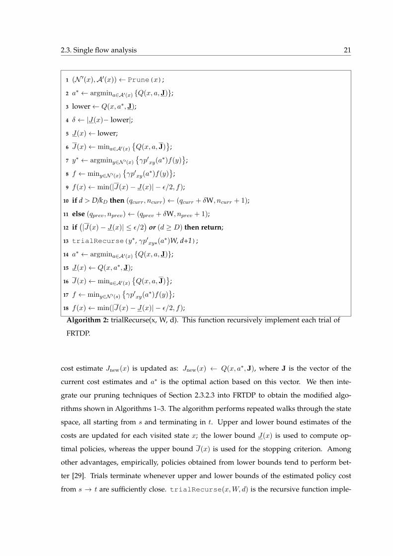
FRTDP.
cost estimate Jnew(x) is updated as: Jnew(x) ← Q(x, a∗,J), where J is the vector of the
current cost estimates and a∗ is the optimal action based on this vector. We then inte-
grate our pruning techniques of Section 2.3.2.3 into FRTDP to obtain the modified algo-
rithms shown in Algorithms 1–3. The algorithm performs repeated walks through the state
space, all starting from s and terminating in t. Upper and lower bound estimates of the
costs are updated for each visited state x; the lower bound J(x) is used to compute op-
timal policies, whereas the upper bound J(x) is used for the stopping criterion. Among
other advantages, empirically, policies obtained from lower bounds tend to perform bet-
ter [29]. Trials terminate whenever upper and lower bounds of the estimated policy cost
from s → t are sufficiently close. trialRecurse(x,W, d) is the recursive function imple-

22 Chapter 2. Cooperator Selection Policies for Multi-hop Ad Hoc Networks
input : x ∈ Soutput: sets N ′(x) and A′(x)
1 amax ← take the χmax nodes in x closest to t;
2 obtain A′(x) from amax;
3 κ← 1; v← 0; V(x)← ∅;
4 forall the elements n in set T −(x) do
5 remove element n from T −(x);
6 v[κ]← psucc(n, amax);
7 κ← κ+ 1;
8 end
9 SortNonDecreasingOrder(v, |T −(x)|);
10 κ← 1; M ← ∆cmax+γmaxx∈S J(x)
;
11 M(x)← 0;
12 repeat
13 M(x) =M(x)(1− v(κ)) + v(κ)∏κ−1z=1(1− v(z));
14 if M(x) ≤M then
15 V(x)← V(x) ∪ m(κ);
16 κ← κ+ 1;
17 end
18 until (M(x) > M) or (κ == |T −(x)|);
19 obtain N ′(x) from x and V(x);
20 return (N ′(x),A′(x));
Algorithm 3: Prune(x). This function implements the state pruning technique of Sec-
tion 2.3.2.3.
menting each trial, starting from node s and performing actions until node t is reached. W
represents the probability (updated recursively) of being in state x. We modified FRTDP
adding the new function Prune(x). In detail, for each state x in a path, according to Propo-
sition 2.3.6 we prune the neighborhood set. These states have a small probability of being
visited and a negligible impact on the performance. Prune(x) works as follows: we se-
lect the χmax nodes in x that are closest to node t (see Remark 2.3.8) and obtain the action

2.3. Single flow analysis 23
set from these. Hence, we use the pruning algorithm of Proposition 2.3.6 considering all
nodes n ∈ T that have not yet decoded the message and pruning those with smaller prob-
ability of being reached at the next transmission. In particular, we add new nodes until
M(x) > M , as dictated by Proposition 2.3.6. In addition, for M(x) we consider the ap-
proximation of Remark 2.3.7. N ′(x), i.e., the neighborhood set, is finally obtained from the
set of selected nodes. The remainder of trialRecurse(s,W, d) is as specified in [29]. In
short, the new optimal action a∗ for state x is selected according to the DP optimal equa-
tion using the latest cost estimates J. Upper and lower bounds are updated according to
the optimality equation as (Jnew(x), Jnew(x)) ← (Q(x, a∗,J),mina∈A′(x)Q(x, a,J)) (lines 3
and 6). The next state to visit, y∗, is picked by maximizing the occupancy times excess uncer-
tainty metric, i.e., W (y)∆(y), where W (y) is the average probability of visiting the state and
∆(y) = (J(y)−J(y))−ǫ/2, represents the accuracy of its cost estimates. This is implemented
as in the original algorithm [29] through a priority function f(y), which is recursively com-
puted for each state. The current trial terminates when the final state is reached (note that
J(t) = J(t) = 0), when a state x having estimates sufficiently close to the optimum cost is
reached, i.e., J(x) − J(x) ≤ ǫ/2 or when the current path length is longer than D. When-
ever the current trial terminates, optimal actions, lower and upper bounds and priority are
updated on the way back along the traversed path from s→ t (lines 14− 18). For the check
on the path length, poor outcome selection early in a trial could lead to traversing a large
number of irrelevant states which take a long time to escape. The check on the maximum
hop length implements the adaptive maximum depth (AMD) trial termination of [29] which
solves this problem cutting excessively long paths.
2.3.2.5 Numerical Results
In this section we provide an example application of the proposed optimization tech-
niques for cooperator selection policies, showing numerical results and obtaining insights
for the low-complexity implementations of Section 2.3.3. We consider the network topology
of Fig. 2.1, where a source node s transmits a message to a destination node t and the re-
maining nodes are available for cooperation. All nodes except the destination are organized
in a number of columns, each comprising five nodes. The inter-column distance d is picked
in the range 45 ÷ 80 m, while the distance between two adjacent nodes in a column is 2 m.
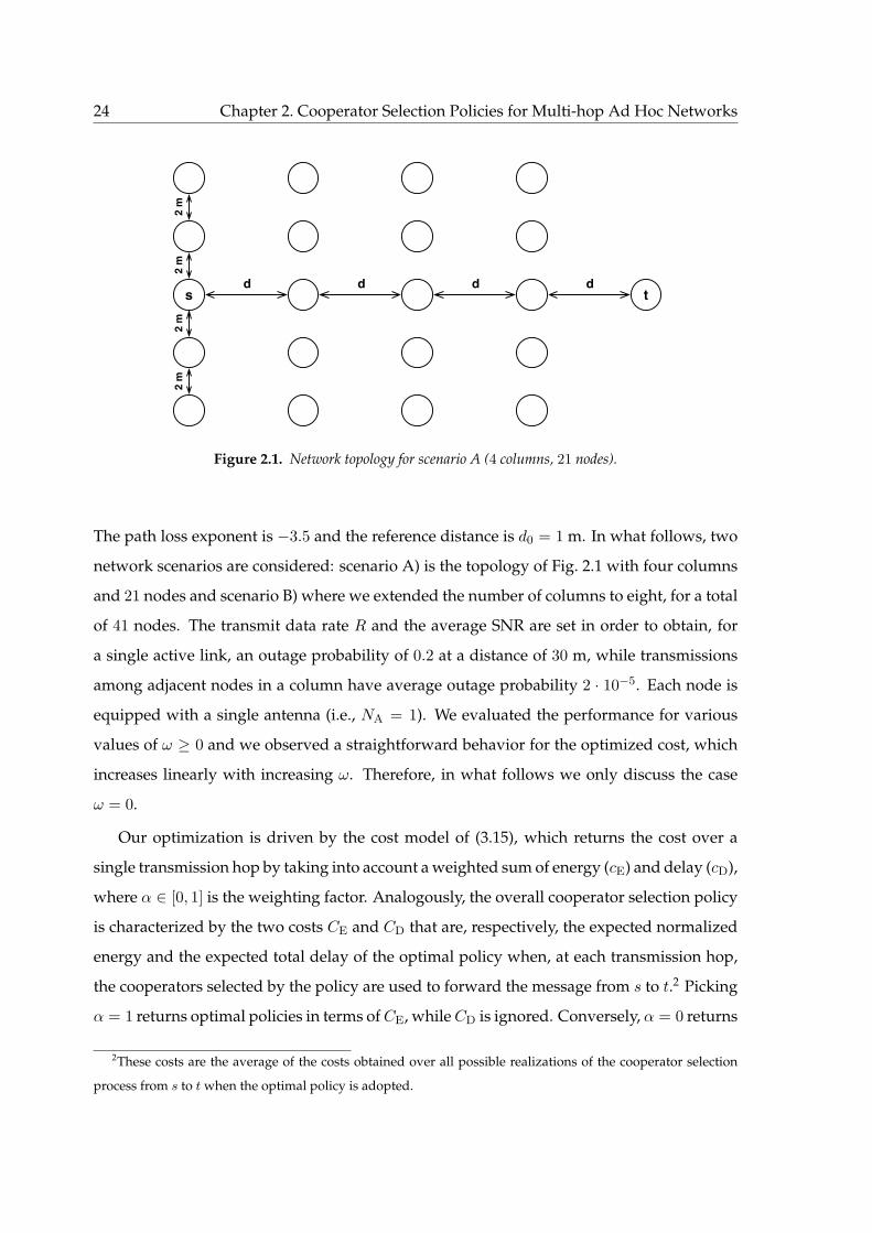
24 Chapter 2. Cooperator Selection Policies for Multi-hop Ad Hoc Networks
s td d d d
2 m
2 m
2 m
2 m
Figure 2.1. Network topology for scenario A (4 columns, 21 nodes).
The path loss exponent is −3.5 and the reference distance is d0 = 1 m. In what follows, two
network scenarios are considered: scenario A) is the topology of Fig. 2.1 with four columns
and 21 nodes and scenario B) where we extended the number of columns to eight, for a total
of 41 nodes. The transmit data rate R and the average SNR are set in order to obtain, for
a single active link, an outage probability of 0.2 at a distance of 30 m, while transmissions
among adjacent nodes in a column have average outage probability 2 · 10−5. Each node is
equipped with a single antenna (i.e., NA = 1). We evaluated the performance for various
values of ω ≥ 0 and we observed a straightforward behavior for the optimized cost, which
increases linearly with increasing ω. Therefore, in what follows we only discuss the case
ω = 0.
Our optimization is driven by the cost model of (3.15), which returns the cost over a
single transmission hop by taking into account a weighted sum of energy (cE) and delay (cD),
where α ∈ [0, 1] is the weighting factor. Analogously, the overall cooperator selection policy
is characterized by the two costs CE and CD that are, respectively, the expected normalized
energy and the expected total delay of the optimal policy when, at each transmission hop,
the cooperators selected by the policy are used to forward the message from s to t.2 Picking
α = 1 returns optimal policies in terms ofCE, whileCD is ignored. Conversely, α = 0 returns
2These costs are the average of the costs obtained over all possible realizations of the cooperator selection
process from s to t when the optimal policy is adopted.

2.3. Single flow analysis 25
optimal policies in terms of CD, ignoring CE. Intermediate values of α lead to suitable
trade-offs between energy and delay. In what follows, optimal policies are obtained setting
γ = 0.99, which is adequate for static networks, see Section 2.3.2. For our FRTDP technique
we set ǫ = 10−3, J(x) = 0, ∀x ∈ S , KD = 1.1 and D0 = 10. For the upper bound J(x) we
considered ∆ = 0.001 and a large initial J(x) = 100, ∀x ∈ S \ t and for these we obtained a
first policy and the corresponding cost J∗p (x), ∀x ∈ S \ t. We thus set J(x)← J∗
p (x)+∆/(1−
γ).
The choice of parameter ∆ is guided by the trade-off between sub-optimality of the pol-
icy and its computational complexity. In detail, when ∆ = 0 our FRTDP optimizer does
not cut any state and finds optimal policies as done by RTDP [27], where J∗(s) is their cost.
When ∆ > 0 some states are instead pruned according to our techniques of Section 2.3.2.3
and our optimizer returns an approximation of the optimal policy, with cost J∗p (s). Note
that setting ∆ > 0 for any given state x reduces the number of neighboring states y and, to
a lesser extent, also reduces the number of states for which the policy is computed, as states
hit with small probability are not considered. As a consequence, the optimal policy is not
calculated for these states. Table 2.1 shows the performance of our FRTDP algorithm as a
function of ∆, for d = 60 m and α = 1 in terms of
1. computational complexity, expressed in terms of number of visited states;
2. estimated failure probability pfail(∆), i.e., the probability of hitting a state for which
our optimizer did not calculate optimal actions;
3. actual cost difference with respect to RTDP, i.e., 100|J∗p (s)− J
∗(s)|/J∗(s);
4. the maximum cost difference between J∗p (s) and J∗(s), as predicted by Theorem 2.3.4,
i.e., 100∆/[J∗p (s)(1− γ)].
We first discuss the results for scenario A. In this case, even a small ∆ = 0.001 suffices to
dramatically reduce the number of visited states, which drops from 1.3 · 109 to 2.2 · 106. For
this ∆, our bounds would predict a maximum additional cost that is just 0.76% larger than
J∗p (S). We note that, for this specific network topology, the solver performance is better than
that predicted by the bound. Also, there is a threshold effect on the number of pruned states
for increasing ∆, which is due to the specific topology under consideration. For scenario B
(41 nodes) the solver fails to obtain policies for ∆ = 0, due to the excessively large number of

26 Chapter 2. Cooperator Selection Policies for Multi-hop Ad Hoc Networks
Table 2.1. Performance of the modified FRTDP optimizer as a function of ∆.
Scenario A: 21 nodes network Scenario B: 41 nodes network
∆ Visited Failure ∆C [%] ∆C [%] Visited Failure ∆C [%]
States Prob. pfail(∆) Actual Predicted States Prob. pfail(∆) Predicted
0 1.3 · 109 0 0.00 — — — —
0.001 2.2 · 106 9.0 · 10−6 0.00 0.76 3.3 · 108 5.0 · 10−6 0.45
0.005 2.2 · 106 9.0 · 10−6 0.00 3.82 3.3 · 108 5.0 · 10−6 2.24
0.01 2.2 · 106 9.0 · 10−6 0.00 7.64 3.3 · 108 5.0 · 10−6 4.49
0.05 2.2 · 106 9.0 · 10−6 0.00 38.18 3.3 · 108 5.0 · 10−6 22.45
0.1 2.2 · 106 9.0 · 10−6 0.00 76.35 3.3 · 108 5.0 · 10−6 44.89
0.5 2.2 · 106 9.0 · 10−6 0.00 381.77 3.3 · 108 5.0 · 10−6 224.46
1 2.2 · 106 9.0 · 10−6 0.00 763.53 3.3 · 108 5.0 · 10−6 448.92
5 1.5 · 106 5.9 · 10−5 5.13 3631.35 2.9 · 108 1.3 · 10−5 2175.95
10 7.0 · 105 3.6 · 10−4 13.88 6704.66 1.6 · 108 2.5 · 10−5 4293.26
states. However, ∆ = 0.001 already provides cooperation policies having a small bounded
additional cost with respect to the unknown optimal performance. We shall observe that the
bounds of Theorem 2.3.4 are asymptotically tight, i.e., they become more accurate as the path
length increases. Finally, we note that pfail(∆) is very small in all cases. These results show
the effectiveness of our technique, which makes it possible to find quasi-optimal policies for
large networks at a reduced complexity.
Fig. 2.2 showsCE andCD as a function of the inter-column distance d for α = 1 (minimum
energy) and α = 0 (minimum delay). Costs are normalized with respect to the cost incurred
for a single packet transmission. We observe that for α = 1 the energy cost CE increases
smoothly with d, while for α = 0 the delay cost CD increases smoothly with time, since a
larger distance d between columns yields higher outage probabilities which, in turn, lead to
longer transmission delays over single hops. In the figure, we also show non targeted costs,
i.e.,CD when the optimization objective corresponds to minimizing the energy consumption
(α = 1) and CE when the objective is the minimization of the delay (α = 0). Non targeted
costs generally increase with increasing d. However, the corresponding curves have an irreg-

2.3. Single flow analysis 27
0
10
20
30
40
50
60
70
45 50 55 60 65 70 75 80
No
rmal
ized
Co
st
Inter-column distance d [m]
CE, α=0CD, α=0CE, α=1CD, α=1
Figure 2.2. Normalized costs CE and CD as a function of d for α = 0 and α = 1. CE and CD are
normalized with respect to the energy spent to transmit a single packet and the message transmission
delay, respectively. Other optimization parameters are: ω = 0, γ = 0.99, ∆ = 0.001 and χmax = 5.
ular behavior as in some cases non-targeted costs decrease with the inter-column distance.
This is due to the fact that the optimization is performed on a discrete set of policies. For
example, when the target cost is CE and d is slightly increased, to counteract the increased
outage probability cooperation may start earlier and involve a larger number of nodes. The
effect of this is twofold: 1) CE is kept as small as possible and 2) the delay is decreased
as more nodes transmit at each hop. Overall, the result is a slight increase in CE (thus the
smooth curve forCE) together with a sudden drop ofCD due to the reduced number of hops
(thus the irregular curve for CD).
To better understand the impact of cooperation in a multihop scenario with optimized
cooperator selection policies, in Fig. 2.3 we show the average number of nodes that transmit
simultaneously, as a function of d and for various values of α. Note that, when the objec-
tive is to minimize the delay, optimal policies tend to maximize the number of cooperating
nodes per hop as the cost in this case is solely given by the number of hops traveled by the
message, irrespective of the number of transmitting nodes within each hop. When mini-
mizing energy, the cost also depends on the number of cooperating nodes within each hop

28 Chapter 2. Cooperator Selection Policies for Multi-hop Ad Hoc Networks
1
1.5
2
2.5
3
3.5
4
4.5
45 50 55 60 65 70 75 80
Co
ncu
rren
t T
ran
smis
sio
ns
per
Ho
p
Inter-column distance d [m]
α = 1 α = 0.4 α = 0.2 α = 0.05
α = 0 1
1.5
2
2.5
3
3.5
4
4.5
45 50 55 60 65 70 75 80
Co
ncu
rren
t T
ran
smis
sio
ns
per
Ho
p
Inter-column distance d [m]
α = 1 α = 0.4 α = 0.2 α = 0.05
α = 0
Figure 2.3. Average number of cooperating nodes as a function of d for different values of α. Other
optimization parameters are: ω = 0, γ = 0.99, ∆ = 0.001 and χmax = 5.
and, as a consequence, the optimal number of cooperating nodes per hop is smaller. Also
in this case we observe an irregular behavior of the curves, which can be explained consid-
ering the discrete nature of the problem. In general, the average number of simultaneous
transmissions decreases with increasing d, as outages occur more often and, in such cases,
less nodes are available for transmission. However, this is true until the cooperation policy
changes, at which point cooperation is forced among a larger number of nodes in order to
minimize the targeted cost. Notably, we can see a close relationship between Fig. 2.3 and the
non-targeted costs of Fig. 2.2: for example, when α = 1 at 58.75 m the average number of
simultaneous transmissions increases from 1.45 to 1.86 (Fig. 2.3) and, at the same time, CD
drops from 8.53 to 6.56 (Fig. 2.2). This corresponds to a forced earlier cooperation among
nodes which causes an increase in CE as well as a subsequent reduction in the number of
hops. Fig. 2.3 also confirms that cooperation is advantageous when multihop is considered
and minimization of energy consumption rather than delay or rate are targeted. As an ex-
ample, for α = 1 the average number of simultaneous transmissions goes from 20% (i.e., 1
transmitting node for d = 45 m over a maximum of χmax = 5 cooperating nodes) to 60%
(i.e., 3 cooperating nodes over χmax = 5). In addition, we observe that the average number

2.3. Single flow analysis 29
10
12
14
16
18
20
22
24
4.5 5 5.5 6 6.5 7 7.5 8 8.5 9
No
rmal
ized
En
erg
y C
ost
, C
E
Normalized Delay Cost, CD
χmax = 2χmax = 3χmax = 4χmax = 5
10
12
14
16
18
20
22
24
4.5 5 5.5 6 6.5 7 7.5 8 8.5 9
No
rmal
ized
En
erg
y C
ost
, C
E
Normalized Delay Cost, CD
χmax = 2χmax = 3χmax = 4χmax = 5χmax = 6
Figure 2.4. CE vsCD for several values of χmax. The curves are obtained for d = 55 m, varying α ∈ [0, 1].
Other optimization parameters are: ω = 0, γ = 0.99, ∆ = 0.001 and χmax ∈ 1, 2, 3, 4, 5, 6.
of cooperating nodes is small with respect to the total number of nodes in the network, thus
it is meaningful to impose a maximum χmax ≪ |T | on the number of cooperating nodes, as
discussed in Section 2.3.2.3.
Fig. 2.4 shows the trade-off between CE and CD as a function of χmax for an inter-column
distance of d = 55 m. The curves are obtained by varying the weighting factor α in [0, 1] and
provide the delay-energy achievable regions, as for a given χmax no policy can obtain a
trade-off point situated below the corresponding optimal curve, while any point above the
optimal curve is achieved by a suitable suboptimal policy. However, this figure provides
even further insights on possible implementations of optimal policies. In fact, for α > 0 set-
ting χmax = 5 already provides most of the benefits of optimal policies in the unconstrained
optimization case (χmax = +∞). This means that complexity of both policy optimization
and network coordination can be reduced at almost no expense in terms of performance.
On the other side, being too restrictive on the number of cooperators yields some perfor-
mance loss, as for example allowing at most 2 cooperating nodes leads to a delay increase
of about 20% and to an increase of energy consumption of about 10%. Note that if coop-
eration is not allowed (i.e., χmax = 1) delay and energy consumption are centered around

30 Chapter 2. Cooperator Selection Policies for Multi-hop Ad Hoc Networks
0
10
20
30
40
50
60
150 200 250 300 350
No
rmal
ized
Co
st
Source-destination distance d [m]
CE, α=0CD, α=0CE, α=1CD, α=1
0
10
20
30
40
50
60
150 200 250 300 350
No
rmal
ized
Co
st
Source-destination distance d [m]
Figure 2.5. Random network: Normalized costs CE and CD as a function of d for α = 0 and α = 1.
point (x, y) = (11.8, 11.8) (out of range in the figure). Therefore, even a minimum level of
cooperation, i.e., between two nodes (χmax = 2), provides a substantial performance advan-
tage. We finally observe that, if at every hop the maximum admissible number of nodes
cooperate, we obtain the delay optimal policy (α = 0). This however comes at the expense
of a high energy consumption. A more judicious choice leads to considerable advantages,
e.g., a delay just 4% over the minimum provides a drop of consumed energy by about 30%.
Finally, we considered random networks with 21 nodes placed within a rectangular sim-
ulation area of 50×d square meters as follows: source and destination are respectively posi-
tioned in the middle of the two opposite 50 m long sizes, whereas the remaining nodes are
randomly placed within the area. Optimization parameters are: ω = 0, γ = 0.99, ∆ = 0.001
and χmax = 5. In the graphs, vertical bars are used to show 95% confidence intervals. For
the random scenario, Fig. 2.5 shows the normalized costs CE and CD as a function of d for
α ∈ 0, 1. Fig. 2.6 instead shows the average number of cooperating nodes for different
values of α. The considerations for these graphs are similar to those made for the previous
plots. As in the previous results, optimal delay strategies (α = 0) entail the largest number
of cooperating nodes. However, differently from the previous results, cooperation is almost
absent when the objective is energy minimization (α = 1). Also, we note that d has a smaller

2.3. Single flow analysis 31
1
1.5
2
2.5
3
3.5
4
4.5
150 200 250 300 350
Co
ncu
rren
t T
ran
smis
sio
ns
per
Ho
p
Source-destination distance d [m]
α = 1 α = 0.4 α = 0.2
α = 0.05α = 0
1
1.5
2
2.5
3
3.5
4
4.5
150 200 250 300 350
Co
ncu
rren
t T
ran
smis
sio
ns
per
Ho
p
Source-destination distance d [m]
α = 1 α = 0.4 α = 0.2
α = 0.05α = 0
1
1.5
2
2.5
3
3.5
4
4.5
150 200 250 300 350
Co
ncu
rren
t T
ran
smis
sio
ns
per
Ho
p
Source-destination distance d [m]
Figure 2.6. Random network: average number of cooperating nodes vs d for different values of α.
impact on the optimal number of cooperating nodes, which is almost constant (compare
Figs. 2.3 and 2.6).
2.3.3 Heuristic Routing Policies
In Section 2.3.2 we presented an analytical solver to find optimal cooperator selection
policies for general topologies. As already stated, the computation of the optimal policies,
according to the objectives introduced in Section 2.3.1, requires a complete knowledge of
the network topology and centralized and off-line computation. In this Section we present
three heuristic policies suitable for a distributed implementation and having a lower com-
putational complexity.
2.3.3.1 K-Closest
The idea of the K-Closest policy is to have a fixed number of relays retransmitting the
message at each time slot and select them according to their distance to the termination
node.
For any node n ∈ N let δn = dn,t be the distance between node n and the termination

32 Chapter 2. Cooperator Selection Policies for Multi-hop Ad Hoc Networks
node t. We assume that each node n can collect this proximity metric from all nodes closer
to the destination than itself. All the nodes that correctly receive the message in time slot i
are ranked by the transmitters according to δn = dn,t, i.e., the ordered set is
Ri = r(1)i , r
(2)i , . . . , r
(|Ri|)i , (2.18)
with
δr(k)i
≤ δr(k+1)i
, k = 1, 2, . . . , |Ri| − 1. (2.19)
With the K-Closest policy at most K nodes cooperate in each time slot, and they are
selected among those closest to the destination. Thus, the set of nodes that cooperatively
transmit at slot i+ 1 is
ai+1 = r(1)i , r
(2)i , . . . , r
(minK,|Ri|)i . (2.20)
Note that if less than K nodes correctly decoded the message at slot i, they are all elected as
relays in the next time slot i+ 1.
2.3.3.2 K-One Step Look Ahead (K-OSLA)
The K-Closest policy exploits the knowledge of the geographical distance between each
potential relay and the termination node t. However, due to the limited amount of infor-
mation that it uses, K-Closest has the potential drawback of choosing relays having a small
number of neighbors in their proximity. Notably, this may increase the average number of
retransmissions necessary to reach the next set of relays. As an example, consider the sce-
nario of Fig. 2.7 where the number of nodes that cooperate for the transmission in each time
slot is K = 2. At a generic time slot i, nodes in the relay set ai cooperatively transmit the
message and nodes in setRi correctly decode it. Following the rationale of K-Closet, nodes
r1 and r2 would be selected as the relays for the next transmission slot i + 1, since they are
the closest nodes to the destination t. However, despite the fact that node r1 is the closest
to t, it does not have additional intermediate nodes between itself and t. Additionally, as
r1 is quite distant from the destination, it will give a small contribution into the successful
forwarding of the packet towards it. Choosing nodes r2 and r3 as the next relay set ai+1 will
instead avoid unnecessary retransmissions by taking advantage of multi-hopping through
the neighboring nodes q and n. In what follows, we extend the K-Closest heuristic with

2.3. Single flow analysis 33
q
r5
r4
r∗
r3
r1
r2
n
t
δq
δn
Figure 2.7. Example of a scenario where K-Closest would choose an unreliable relay set.
a suitable metric, which keeps into account the presence of neighboring nodes in order to
avoid the discussed drawback.
Formally, let q ∈ ai be a node that transmits the message at slot i and n be a candidate
node for the (cooperative) transmission of the message in the next time slot i + 1. The
difference between the distances of node q and node n with respect to the termination node
is denoted as
gq,n = δq − δn , (2.21)
which describes the geographical advancement toward t provided by n. For each node
q ∈ N we can also compute the expected maximum advancement toward t provided only
by node q without the support of other cooperating nodes, i.e.
gq =∑
n:δn≤δq
gq,n[1− pout(q, n)]∏
m:δm≤δn
pout(q,m) . (2.22)
This equation can be better understood if we consider the scenario in Fig. 2.7. In this exam-
ple, we have that the maximum expected advancement toward t provided by a transmission
from node q is determined as a weighted sum of the geographical advancements provided
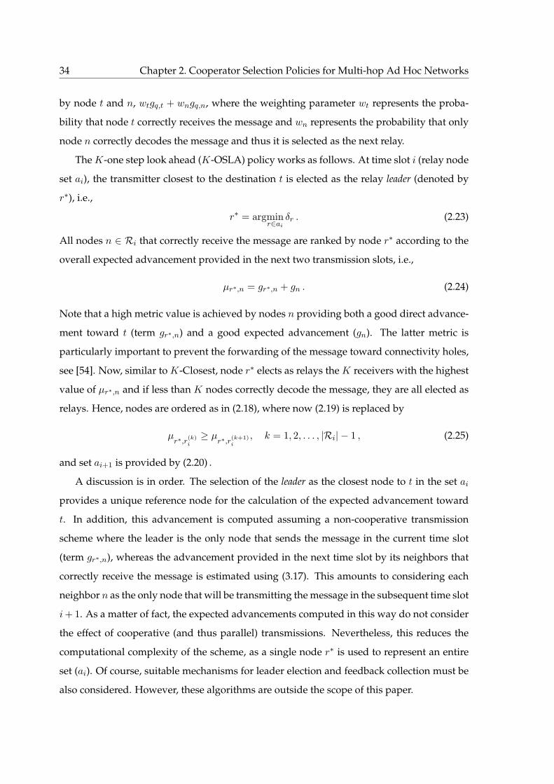
34 Chapter 2. Cooperator Selection Policies for Multi-hop Ad Hoc Networks
by node t and n, wtgq,t + wngq,n, where the weighting parameter wt represents the proba-
bility that node t correctly receives the message and wn represents the probability that only
node n correctly decodes the message and thus it is selected as the next relay.
TheK-one step look ahead (K-OSLA) policy works as follows. At time slot i (relay node
set ai), the transmitter closest to the destination t is elected as the relay leader (denoted by
r∗), i.e.,
r∗ = argminr∈ai
δr . (2.23)
All nodes n ∈ Ri that correctly receive the message are ranked by node r∗ according to the
overall expected advancement provided in the next two transmission slots, i.e.,
µr∗,n = gr∗,n + gn . (2.24)
Note that a high metric value is achieved by nodes n providing both a good direct advance-
ment toward t (term gr∗,n) and a good expected advancement (gn). The latter metric is
particularly important to prevent the forwarding of the message toward connectivity holes,
see [54]. Now, similar to K-Closest, node r∗ elects as relays the K receivers with the highest
value of µr∗,n and if less than K nodes correctly decode the message, they are all elected as
relays. Hence, nodes are ordered as in (2.18), where now (2.19) is replaced by
µr∗,r
(k)i
≥ µr∗,r
(k+1)i
, k = 1, 2, . . . , |Ri| − 1 , (2.25)
and set ai+1 is provided by (2.20) .
A discussion is in order. The selection of the leader as the closest node to t in the set ai
provides a unique reference node for the calculation of the expected advancement toward
t. In addition, this advancement is computed assuming a non-cooperative transmission
scheme where the leader is the only node that sends the message in the current time slot
(term gr∗,n), whereas the advancement provided in the next time slot by its neighbors that
correctly receive the message is estimated using (3.17). This amounts to considering each
neighbor n as the only node that will be transmitting the message in the subsequent time slot
i+ 1. As a matter of fact, the expected advancements computed in this way do not consider
the effect of cooperative (and thus parallel) transmissions. Nevertheless, this reduces the
computational complexity of the scheme, as a single node r∗ is used to represent an entire
set (ai). Of course, suitable mechanisms for leader election and feedback collection must be
also considered. However, these algorithms are outside the scope of this paper.

2.3. Single flow analysis 35
2.3.3.3 η-dynamic One Step Look Ahead (η-dOSLA)
Both K-Closest and K-OSLA always select a fixed number of relays, potentially leading
to an unnecessary waste of energy because also nodes that give a marginal contribution to
the cooperative routing performance may be selected. In what follows, we extend the K-
OSLA heuristic to take into account the impact of cooperation and let the number of relays
be dynamic.
For the η-dynamic one step look ahead (η-dOSLA) policy, we first define η ∈ [0, 1] as
a parameter used to dynamically tune the number of cooperating nodes, as we will detail
later. η-dOSLA uses the geographical advancement metric of (3.17) and, after set Ri has
been ordered according to the metric µr∗,n of (2.24), the set ai+1 is built iteratively as follows.
Node r∗ starts by initializing the set ai+1 so that it only contains the node with the highest
rank
ai+1 = r(1)i . (2.26)
Then, r∗ calculates the expected advancement provided by the current set ai+1 with respect
to the highest rank node r(1)i as
γai+1 =∑
n:δn≤δr(1)i
gr(1)i ,n
[1− pout(ai+1, n)]∏
m:δm≤δn
pout(ai+1,m) . (2.27)
Comparing (2.27) with (3.17) we observe that, while in (3.17) the advancement is computed
ignoring the cooperation of other nodes in ai+1, γai+1 in (2.27) it includes the effects of the
cooperation among all the nodes in the set ai+1, which is gradually populated. Then, the
normalized expected advancement is computed as
gai+1 =γai+1
δr(1)i
, (2.28)
which represents the expected fraction of the distance δr(1)i
covered by the cooperative trans-
mission of the nodes in ai+1.
If gai+1 ≥ η the procedure terminates. Otherwise, node r∗ adds to set ai+1 the next
node in the ordered sequence Ri and recalculates the normalized expected advancement
provided by all nodes in the new set ai+1. At the generic iteration v, we have
ai+1 = r(1)i , r
(2)i , . . . , r
(v)i . (2.29)
The iterative process is terminated either when gai+1 ≥ η or when v = |Ri|.
36 Chapter 2. Cooperator Selection Policies for Multi-hop Ad Hoc Networks
2.3.3.4 Practical Considerations
It can be noted that all the proposed algorithms are based on a distance metric between
each node and the destination t. This is similar to the forwarding paradigm of geographi-
cal routing in wireless networks (see for example [55] and [56]), where it is assumed that
each node is aware of its own position (e.g., exploiting GPS or some distributed localization
service) and that the source is aware of the position of the destination. We make the same
assumptions here, so that each node n can determine its distance from the destination δn
and exchange it with the other nodes of the network when needed. In this way, at each
time slot i, we only require the knowledge of the local topology (i.e., Ri and δr, ∀ r ∈ Ri)
to determine the current relay set. Starting from these assumptions, the complexity of the
proposed techniques varies and is represented by
• K-Closest: at each time slot i, the current transmitters order the set Ri according
to (2.19), which has a complexity of O(|N | log(|N |));
• K-OSLA: each node needs to compute the maximum expected advancement (3.17),
which has a complexity ofO(|N |2). Then, at each time slot i, the current relay leader r∗
orders the setRi according to (2.25), which has a complexity of, at most,O(|N | log(|N |)).
• η-dOSLA: each node needs to compute the maximum expected advancement (3.17),
which has a complexity of O(|N |2). At each time slot i, the current relay leader r∗
orders the setRi according to (2.25), which has a complexity ofO(|N | log(|N |)). More-
over, r∗ iteratively builds the relay set ai+1. At each iteration, node r∗ computes the
expected advancement provided by the current relay set ai+1 (i.e., (2.27)), which as
a complexity of O(|N |2). The maximum number of iterations required to compute
the next relay set is |N | − 2 and thus, computing the next relay set has a complexity
O(|N |3).
Moreover, for a practical implementation of the proposed techniques, additional feedback
mechanisms for packet decoding, relays selection and neighbor discovery must be designed.
These mechanisms are out of scope for this work since our primary objective is investigat-
ing the effectiveness of different relay ranking criteria when used within an opportunistic
routing protocol.

2.3. Single flow analysis 37
0
10
20
30
40
50
60
70
80
90
150 200 250 300 350
No
rmal
ized
Co
st
Source-destination distance d [m]
0
10
20
30
40
50
60
70
80
90
150 200 250 300 350
No
rmal
ized
Co
st
Source-destination distance d [m]
K-Closest (K=5)K-OSLA (K=5)
η-dOSLA (η=1)Delay optimal (α=0)
Figure 2.8. Normalized energy and delay costs as a function of d for optimal and heuristic policies, when
the objective is delay minimization. Solid line: delay cost; dashed line: energy cost.
2.3.3.5 Numerical results
In this section we show numerical results of the network performance attained by the
proposed heuristic schemes. All the results of this section have been obtained using a C++
simulator that assesses the performance of each algorithm using the Monte Carlo method.
In the following graphs, we compare the delay and energy costs of the heuristic policies
against the optimal policies obtained in Section 2.3.2. In particular, we compare the perfor-
mance of the distributed heuristic algorithms of Section 2.3.3 against the curves in Fig. 2.5
that considers random networks with 21 nodes placed within a rectangular area of 50 × d
square meters as follows. Source and destination nodes are placed in the middle of the two
opposite 50 m long sizes, therefore source and destination nodes are at a distance d. All
the remaining nodes are randomly positioned within the area. Moreover, since the curves
of Fig. 2.5 are obtained when the maximum number of nodes that can cooperatively broad-
cast the message in a particular hop is set at χmax = 5, for comparison purposes, we apply
the same limitation to the heuristic policies proposed in Section 2.3.3. This limitation im-
plies K ≤ χmax for policies K-Closest and K-OSLA, while for η-dOSLA we have to add

38 Chapter 2. Cooperator Selection Policies for Multi-hop Ad Hoc Networks
0
5
10
15
20
25
30
35
150 200 250 300 350
No
rmal
ized
Co
st
Source-destination distance d [m]
0
5
10
15
20
25
30
35
150 200 250 300 350
No
rmal
ized
Co
st
Source-destination distance d [m]
K-Closest (K=1)K-OSLA (K=1)
η-dOSLA (η=0.1)Energy optimal (α=1)
Figure 2.9. Normalized energy and delay costs as a function of d for optimal and heuristic policies, when
the objective is energy minimization. Solid line: delay cost; dashed line: energy cost.
the additional constraint that at most χmax nodes can cooperate at each hop. Note that this
constraint implies that |ai| ≤ χmax and possibly leads to cases where gai < η, see (2.28). In
all the results of this section we fix ω = 0, the path loss exponent is κ = 3.5 and we set the
data rate R and the average signal to noise ratio in order to obtain, for a single active link,
an outage probability of 0.2 at a distance of 30 m, in accordance with the simulation scenario
of Fig. 2.5.
Fig. 2.8 shows the energy and delay costs when the optimization objective is delay min-
imization. The curves in this figure have been obtained setting α = 0 in the cost function
(3.15), K = χmax and η = 1 and varying the distance d between the source and the desti-
nation. We observe that for d ≤ 200 m all the schemes provide similar delay costs, while
heuristic policies return a slightly higher energy consumption with respect to optimal poli-
cies. When d increases, we see that K-Closest returns the worst performance in term of both
energy and delay costs, while K-OSLA slightly outperforms K-Closest, and η-dOSLA still
approaches the optimal performance with a delay increase of 22% and an energy increase
of 10% in the worst case. Similar results are obtained in Fig. 2.9, where the optimization
criterion is energy minimization. In this figure we set α = 1, K = 1 and η = 0.1. Note that

2.3. Single flow analysis 39
0
10
20
30
40
50
60
70
10 20 30 40 50 60
No
rmal
ized
Co
st
Number of Nodes
0
10
20
30
40
50
60
70
10 20 30 40 50 60
No
rmal
ized
Co
st
Number of Nodes
η-dOSLA (η=1)K-OSLA (K=5)
K-Closest (K=5)K-OVM (K=5)
Figure 2.10. Normalized energy and delay costs as a function of the number of nodes in the network for
heuristic policies and OVM, when the objective is delay minimization. Solid line: delay cost; dashed line:
energy cost.
setting K = 1 implies that no cooperation is allowed in both K-Closest and K-OSLA (and
thus energy and delay costs coincide, see (3.15)), while η > 0 allows the simultaneous trans-
mission from different nodes. As before, η-dOSLA outperforms K-Closest and K-OSLA
and, despite attaining higher energy expenditure, achieves better delay performance with
respect to the optimal policies (note that this is allowed because the optimization criterion
of the optimal policies is energy minimization).
In addition, we compared the performance of the proposed heuristic policies with that
of the opportunistic virtual MISO (OVM) protocol proposed in [34]. OVM considers that, at
each hop, the current transmitter can be assisted by one relay. Since in our heuristic policies
we can tune the number of cooperating nodes, we extended OVM in a similar way. We call
this implementation K-OVM, where K represents the maximum number of nodes that can
cooperatively forward the message to the next hop. Here we consider the same network
structure of the previous figures, except for the size of the rectangular area, which is now
150× 150 square meters.
Fig. 2.10 shows the energy and delay costs as a function of the number of nodes in the

40 Chapter 2. Cooperator Selection Policies for Multi-hop Ad Hoc Networks
η = 0.1
η = 1
K = 2
K = 5
K = 2
K = 5
8
10
12
14
16
18
20
22
4 5 6 7 8 9 10 11 12 13 14 15
No
rmal
ized
En
erg
y
Normalized Delay
!-dOSLAK-OSLA
K-ClosestK-OVM
Figure 2.11. Energy as a function of the delay for heuristic policies and OVM. The curves are obtained for
20 nodes, varying η ∈ (0, 1] and K ∈ 2, 3, 4, 5.
network when the objective is delay minimization. In this figure, the curves have been ob-
tained setting K = 5 and η = 1. We see that our schemes outperform OVM in all the consid-
ered scenarios. In addition, we observe that K-OSLA and η-dOSLA perform slightly better
than K-Closest when the number of nodes is less than 30, while all the three schemes per-
form closely for higher node densities. This is reasonable since the additional information
about the expected advancement exploited by K-OSLA and η-dOSLA is meant to prevent
the forwarding of the message toward connectivity holes, that are more frequent for sparser
networks.
In Fig. 2.11, we set the number of nodes to 20 and we obtained the points by varying η
in (0, 1] for η-dOSLA and K in 2, 3, 4, 5 for K-Closest, K-OSLA and K-OVM. We observe
that our schemes outperformK-OVM in terms of delay cost for all the values ofK and η. As
expected, K-OSLA improves over K-Closest in terms of both energy and delay, especially
for small values of K (K ≤ 3 in the figure), while for K ∈ 4, 5 it provides a small delay
improvement at the expense of a slight increase in energy expenditure. In addition, we
observe that η-dOSLA outperforms all the other schemes and allows for a more refined
tuning between energy and delay. Finally, it is interesting to notice that while in our schemes

2.4. Multiple flows analysis 41
increasing the number of cooperating nodes leads to a decrease in the delay experienced by
the message and a consequent increase in the energy consumption, in K-OVM increasing
K has the effect of simultaneously decreasing both energy and delay and this reflects the
different working principles of the two schemes.
2.4 Multiple flows analysis
In Section 2.3 we studied the behavior of a wireless network in which, at each time slot,
only a single flow is present in the network. In this Section we extend the previous results to
a more general case, in which an arbitrary number of concurrent flows is active in the net-
work at any time, and we devise an efficient algorithm for computing optimal interference-
aware policies. The extension to multiple flows is not straightforward from the single flow
case, because of the exponential nature of the problem, and require a complete redesign of
the network model and the choice of a suitable stochastic optimization technique.
2.4.1 System model, adaptation to multiple flows
The system model of Section 2.2 needs to be modified in order to take into account the
presence of multiple flows and the interference between them. To this end, consider a wire-
less network consisting of a setN of nodes spread out according to any distribution. Time is
slotted with a slot corresponding to the fixed transmission time of a packet and all nodes are
synchronized at the slot level. The nodes are grouped into clusters during the network ini-
tialization phase according to any clustering algorithm. Moreover, only the nodes belonging
to the same cluster can cooperate for the transmission of a packet. As already stated in this
Chapter, when multiple nodes cooperate, they transmit the same packet simultaneously, i.e.,
in the same slot. From the original network nodes, we build a superimposed structure of
virtual nodes on which we perform our optimization. A virtual node can be of three types:
T1) a single network node, T2) a cluster of network nodes or T3) a subset of the nodes in a
cluster.
We obtain a weighted directed graph G = (V,E), where V is the set of virtual nodes and
E is the set of edges, where each edge (u, v) ∈ E represents a possible communication link
between any two given virtual nodes in V . Moreover, each edge (u, v) ∈ E is weighted with
a cost cuv according to a metric that takes into account the energy used for transmission,

42 Chapter 2. Cooperator Selection Policies for Multi-hop Ad Hoc Networks
the reliability of the link and the entangled delay. In G, transmissions and receptions occur
between virtual nodes and once a packet is successfully received at a given virtual node, all
the actual nodes therein will cooperate for its subsequent transmission in a future slot. Let
puv be the probability that the packet transmitted by virtual node u is successfully received
by all nodes in v, which can be easily derived from the link model of Section 2.2.2 and the
corresponding outage probability definition of Section 2.2.3, as
puv =∏
n∈N s.t.n∈v
(1− pout(u, n)) . (2.30)
We thus set
cuv =
c u = v
βc+ (1− β)wupuv
u 6= v ,(2.31)
where c represents a delay cost for the transmission of one packet in the corresponding slot,
wu is the number of actual nodes in the virtual node u and β ∈ [0, 1]. Note that u = v means
that the packet is not transmitted during a time slot; the virtual node holds the packet and
will transmit it in a future slot as dictated by the optimal transmission schedule. In this case,
we incur the positive delay cost c so as to avoid unnecessary self-loops during the optimiza-
tion process, which lead to erroneous solutions. Note that, considering the use of Stop and
Wait ARQ for failed packets, 1/puv is the average number of transmissions for the success-
ful delivery of a packet over link (u, v).3 Thus, c/puv and wi/puv respectively correspond to
the average delay and the average energy expenditure for the successful transmission of the
packet over this link.
A demand is a pair of nodes (s, f) with s, f ∈ V and s 6= f which indicates node s
as the source for a packet to be delivered to the final (or destination) node f . The set of
demands is denoted by D = (s1, f1), (s2, f2), . . . , (sK , fK). We say that a subgraph H ⊆ G
connects a demand (s, f) when it contains a path from s to f , i.e., a sequence of edges
(s, n1), (n1, n2), . . . , (nℓ−1, nℓ), (nℓ, f), where each edge corresponds to the transmission in
a particular time slot. Note that source s and destination f are virtual nodes of type T1,
whereas ni with i = 1, 2, . . . , ℓ are virtual nodes which, when cooperative transmissions
occur, can also be of type T2 and T3. Packet transmissions occur synchronously according
to the slotted time structure. Hence, the transmission of a packet through a path that is ℓ+1
3We neglect the transmission of acknowledgments.

2.4. Multiple flows analysis 43
hops long, with ℓ ≥ 0, entails a minimum of ℓ + 1 time slots. Note that more than ℓ + 1
time slots may be needed for the transmission over this path as the packet may stop at some
nodes during certain time slots to avoid interference with other flows. Finally, it is assumed
that each demand d ∈ D is composed of a single information packet.
Given any two nodes n,m ∈ N , we indicate with dmax the maximum distance at which
a packet transmitted from n is received at m with a probability larger than or equal to δth
(with δth > 0 and small), or equivalently having an outage probability smaller than or equal
to 1− δth. In other words, dmax is considered as the maximum distance at which two nodes
can reliably communicate. Also, we let αdmax with α ≥ 1 be the interference range, i.e., the
maximum distance for which the transmission from a node i interferes with a concurrent
reception at a node j.
To quantify the interference among paths in the presence of cooperative transmissions
we need to consider the transmission of virtual nodes. Specifically, we say that two paths
interfere with one another in a given time slot when the transmission of one virtual node
in the first path interferes with the transmission of another virtual node of the second path.
Formally, let nu → nv and nh → nk be the transmissions on the first and second path,
respectively, where nu, nv, nh, nk ∈ V . In this work we consider that nu → nv interferes with
nh → nk if either of the following conditions is verified:
C1. There exists at least a pair of nodes with the first being in nu and the second in nk with
distance smaller than or equal to αdmax. In this case the transmission from nu would
interfere with the reception at nk.
C2. There exists at least a pair of nodes with the first being in nh and the second in nv with
distance smaller than or equal to αdmax. In this case the transmission from nh would
interfere with the reception at nv.
Following this rationale, we define an interference graph I = (V,A), having as vertices the
virtual nodes in V . The set A contains the edges and is obtained connecting any two virtual
nodes nu, nv ∈ V if there exists at least a pair of nodes with the first being in nu and the
second in nv with distance smaller than or equal to αdmax.
We remark that alternative and more precise conditions for the definition of the interfer-
ence graph are possible. This definition of interference is adopted here as it is computation-
ally tractable, while providing a reasonable approximation of the actual interference among

44 Chapter 2. Cooperator Selection Policies for Multi-hop Ad Hoc Networks
virtual nodes. Note that these conditions do not impact the correctness of our optimization
algorithm, which works for any given interference graph.
2.4.2 Joint Optimization of Routing and Scheduling
The goal of this work is to find the minimum weight set of non-interfering paths connect-
ing all demands.
For each demand d ∈ D, let sd and fd be its source and destination nodes, respectively.
Moreover, for each edge (u, v) ∈ E, let xduv(i) be 1 if the packet associated with demand
d is transmitted over the link (u, v) in time slot i (transmission u → v with u, v ∈ V ) and
xduv(i) = 0 otherwise. In formulas, our minimum weight set problem can be written as:
min∑
d∈D
∑
(u,v)∈E
∑
t≥0
cuvxduv(i) (2.32a)
subject to:
∑
(v,h)∈E|xduv(t−1)=1
xdvh(t) = 1, d ∈ D, ∀ i (2.32b)
xduv(i) + xd′
lm(i) ≤ 1, (l, v) ∈ A and (u,m) ∈ A
d, d′ ∈ D, d 6= d′, ∀ i (2.32c)
∑
(u,v)∈E
xduv(i1) = 1, d ∈ D, u = sd, i1 ≥ 0 (2.32d)
∑
(v,u)∈E
xdvu(i2) = 1, d ∈ D, u = fd, i2 ≥ 0 (2.32e)
xduv(i) ∈ 0, 1, (u, v) ∈ E, d ∈ D, ∀ i . (2.32f)
The objective function (2.32a) corresponds to minimizing the total cost incurred by the
transmissions along the paths that connect each demand in D. The constraints are:
• Paths creation: for each demand d ∈ D and for any time slot t we have the following
two cases: (1) the packet is not transmitted by the current virtual node v, i.e., xdvh(i) = 0
for h 6= v and xduv(i) = 1 or (2) the packet is transmitted from v to h 6= v, i.e., xdvh(i) = 1
for h 6= v and xdvv(t) = 0. (2.32b) follows as these two cases are mutually exclusive.

2.4. Multiple flows analysis 45
• Interference avoidance: for each pair of interfering links and for any time slot t, at
most one of the two links can be active (2.32c).
• Source: for each demand d ∈ D, there must be a time slot i1 ≥ 0 from which the path
that connects the demand d starts (2.32d).
• Destination: for each demand d ∈ D, there must be a time slot i2 ≥ i1 (this is ensured
by condition (2.32b)) from which the path that connects the demand d ends (2.32e).
• Link: for each demand and time slot a particular link can only be either active or silent
(2.32f).
The presented optimization problem has a linear objective function and linear constraint
functions, thus it can be solved using a linear optimization algorithm [57]. The problem has
many variables and constraints for each time slot i, so the time and the amount of memory
required to find the optimal solution can be extremely large. To deal with these facts we
derived an alternative formulation of the problem, which can be solved faster and requiring
a reduced amount of memory.
2.4.3 Shortest Path Formulation
First of all we introduce the notion of state. The system state in the generic time slot t is
an orderedK-tuple a(t) = (a1, a2, . . . , aK), ad ∈ V which, for each demand d ∈ D represents
the virtual node ad that
• has the packet associated with demand d,
• is allowed to transmit in this slot.
A transition from state a = (a1, a2, . . . , aK) to state b = (b1, b2, . . . , bK) is possible only if the
following two conditions are satisfied:
1) each of the nodes bj can be reached by a transmission from aj , i.e., (aj , bj) ∈ E,
2) no interference arises, i.e., (al, bj) /∈ A, ∀ l 6= j.
The cost associated with the transition from state a to state b is calculated using (2.31) as
c(a→ b) =k∑
j=1
cajbj . (2.33)

46 Chapter 2. Cooperator Selection Policies for Multi-hop Ad Hoc Networks
Using these definitions, the problem of finding the minimum weighted set of non-interfering
paths that connect all demands inD can be seen as a shortest path problem from the starting
state s = (s1, s2, . . . , sK) to the termination state f = (f1, f2, . . . , fK). Note that sj and fj
are all virtual nodes of type T1, i.e., they all correspond to actual network nodes, whereas
the intermediate virtual nodes along the path can be of any type. Also, we remark that fj
is the termination sub-state associated with the jth demand, i.e., when the packet of the jth
demand arrives at the virtual node fj this demand is delivered and no further transmissions
occur. Given this, the problem is equivalent to the single-pair shortest path problem [44] that
is studied in graph theory and can be solved, for example, using Dijkstra’s algorithm. Due
to the large number of states that are generated (the number of states in a(i), i.e., |V |K) it is
wise to solve our problem using an adequate algorithm in order to limit the time complexity
and the memory space required to solve it. A good choice is the A∗ search algorithm [58] that
speeds up the search using heuristics, whilst returning the optimal policy.
A∗ is a best-first graph search algorithm that finds the minimum-cost path on a graph
from a given initial vertex s to one final vertex f . Since in our case each vertex is a state of
our problem we will use the two terms interchangeably. A∗ uses a distance-plus-cost heuristic
function to determine the order in which the search visits the states. For any given state x
this function is given by the sum of two functions:
1. The path-cost function: given by the accumulated cost from s to x, usually denoted by
g(x).
2. An admissible heuristic cost: given by an admissible heuristic estimate of the mini-
mum cost from x to f , usually denoted by h(x).
The term admissible means that h(x) must be smaller than or equal to the minimum actual
cost from x to f , calculated over all possible paths. In our problem, for any given state x
we compute the path-cost function g(x) as the sum of the costs incurred in the path from s
to x. Note that this quantity can be accumulated during the search. For h(x) we proceed as
follows:
1. Given x = (x1, x2, . . . , xK) and the final state f = (f1, f2, . . . , fK), for each xj , we
compute the minimum cost-path connecting xj to the corresponding final node fj .
This is accomplished using the Dijkstra’s algorithm. Let h(xj) be the cost of this path.

2.4. Multiple flows analysis 47
250 m
25
0 m
10 m
8 m 50 m
Figure 2.12. Network scenario.
2. h(x) is obtained as h(x) =∑K
j=1 h(xj).
Note that the obtained cost corresponds to the exact minimum cost when the interference is
neglected. Hence, h(x) is a lower bound of the cost in the presence of interference and the
heuristic is admissible.
As an example of the effectiveness of A∗ in reducing the number of states to be visited,
we considered a network with 9 clusters of nodes with 3 nodes in each cluster and K = 3
demands. For this network we have that |V | = 63 and the total number of states is |V |K =
250047. A∗ allowed the solution of this problem visiting less than 6000 states in all our
results, i.e., less than 2.4% of the total number of states.
2.4.4 Numerical results
In this section we discuss some numerical results obtained using the optimization ap-
proach of Section 2.4.3 on the network topology of Fig. 2.12. The considered network is
composed of 9 clusters of nodes with three nodes per cluster, where clusters are equally
spaced in a grid. Therefore from each cluster we obtain 7 virtual nodes. For the following
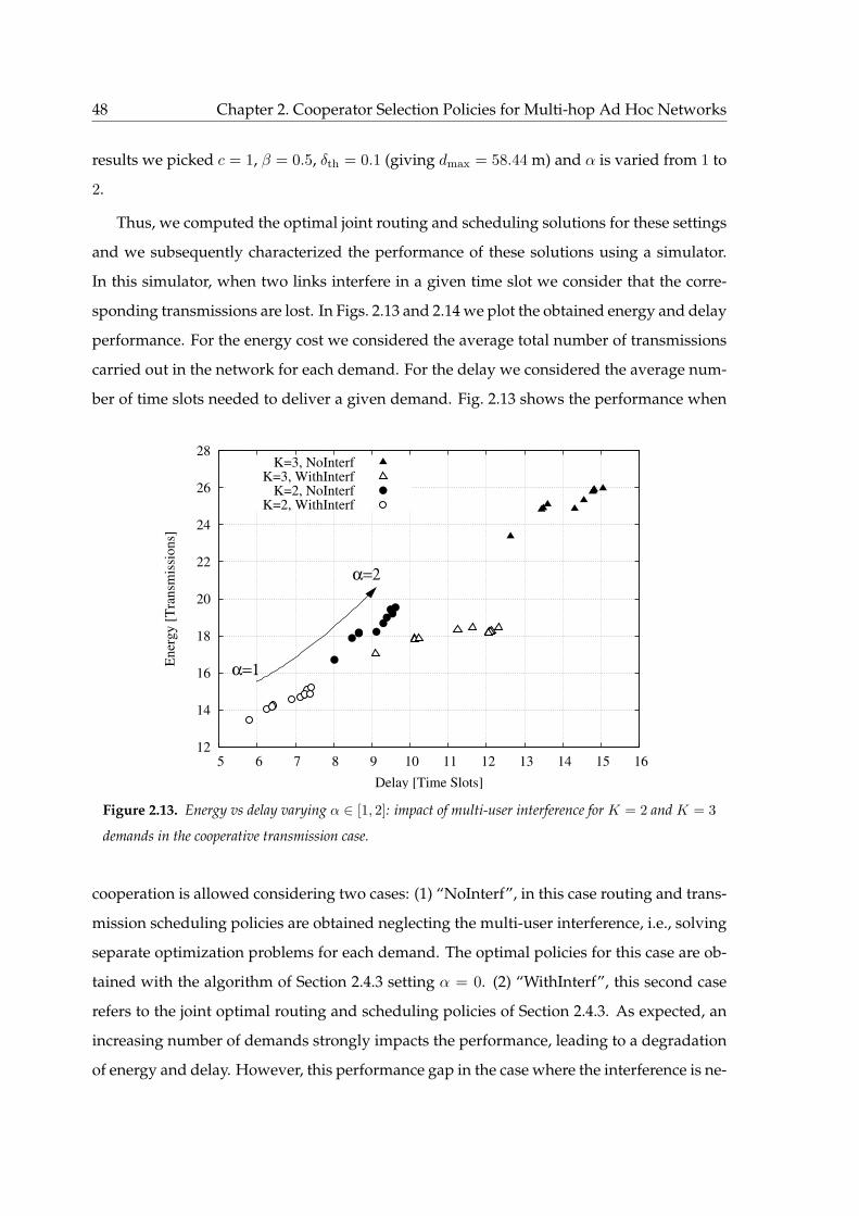
48 Chapter 2. Cooperator Selection Policies for Multi-hop Ad Hoc Networks
results we picked c = 1, β = 0.5, δth = 0.1 (giving dmax = 58.44 m) and α is varied from 1 to
2.
Thus, we computed the optimal joint routing and scheduling solutions for these settings
and we subsequently characterized the performance of these solutions using a simulator.
In this simulator, when two links interfere in a given time slot we consider that the corre-
sponding transmissions are lost. In Figs. 2.13 and 2.14 we plot the obtained energy and delay
performance. For the energy cost we considered the average total number of transmissions
carried out in the network for each demand. For the delay we considered the average num-
ber of time slots needed to deliver a given demand. Fig. 2.13 shows the performance when
12
14
16
18
20
22
24
26
28
5 6 7 8 9 10 11 12 13 14 15 16
Ener
gy [
Tra
nsm
issi
ons]
Delay [Time Slots]
K=3, NoInterfK=3, WithInterf
K=2, NoInterfK=2, WithInterf
α=1
α=2
Figure 2.13. Energy vs delay varying α ∈ [1, 2]: impact of multi-user interference for K = 2 and K = 3
demands in the cooperative transmission case.
cooperation is allowed considering two cases: (1) “NoInterf”, in this case routing and trans-
mission scheduling policies are obtained neglecting the multi-user interference, i.e., solving
separate optimization problems for each demand. The optimal policies for this case are ob-
tained with the algorithm of Section 2.4.3 setting α = 0. (2) “WithInterf”, this second case
refers to the joint optimal routing and scheduling policies of Section 2.4.3. As expected, an
increasing number of demands strongly impacts the performance, leading to a degradation
of energy and delay. However, this performance gap in the case where the interference is ne-

2.4. Multiple flows analysis 49
glected is almost doubled for both metrics. Fig. 2.14 illustrates the benefits brought about by
15
20
25
30
35
5 10 15 20 25 30 35
Ener
gy [
Tra
nsm
issi
ons]
Delay [Time Slots]
NoInterf, CoopWithInterf, Coop
NoInterf, NoCoopWithInterf, NoCoop
α=1
α=2
Figure 2.14. Energy vs delay varying α ∈ [1, 2]: impact of cooperative transmission for K = 3 demands.
cooperating transmissions (“Coop” in the figure). First of all, considering the interference in
the routing/scheduling policy also leads to better results for both performance metrics and
the benefits are substantially larger when nodes cooperate. As expected, the best policies are
those accounting for cooperation and interference (“WithInterf, Coop”) that, when the inter-
ference is high (i.e., α = 2), lead to a three fold reduction of both energy and delay. Another
interesting observation is that cooperation allows for additional savings in terms of energy
and delay with respect to “WithInterf, NoCoop”, where the interference is considered but
the cooperation is neglected.
In non cooperative systems the interference can be neglected when interference and
transmission ranges are equal (see Fig. 2.14 with α = 1). This is no longer valid when
nodes cooperate. In fact, in this case, even when α = 1 the actual transmission range of
multiple cooperating nodes becomes higher than that of a single transmitting node, leading
to a larger interference area and thus exacerbating the negative effect of interfering trans-
missions. On the other hand, when interference is considered in the optimization process,
cooperation can provide further benefits of up to 25% and 58% for the energy and delay,
respectively (see “WithInterf, NoCoop” versus “WithInterf, Coop” in Fig. 2.14).

50 Chapter 2. Cooperator Selection Policies for Multi-hop Ad Hoc Networks
2.5 Conclusions
In this Chapter we first found optimal cooperator selection policies for multihop net-
works with MIMO transmissions and a single flow. The cooperator selection process was
modeled for arbitrary topologies through a suitable Markov chain. Hence, this chain was
reduced according to an original pruning technique which cuts states with negligible im-
pact on the optimal solution. Thus, we integrated this pruning technique into an advanced
solver based on real time dynamic programming and we showed the effectiveness of this
approach in terms of goodness of the policy and computational complexity. Our solver finds
policies within an additional cost bounded with respect to the optimal and allows to derive
the Pareto efficient frontier in terms of transmission cost vs delay for arbitrary networks.
Through selected application examples we discussed the impact of: 1) the set of nodes that
cooperate at each transmission opportunity, 2) the selection of the optimization criteria, i.e.,
energy vs delay minimization and 3) the maximum number of nodes that are allowed to
cooperate.
We then proposed three algorithms for the selection of cooperating nodes in multihop
wireless networks in a distributed fashion. The aim of these policies is the minimization of
a cost obtained as a linear combination of delay and energy consumption, as for the opti-
mal policies. The three policies allow the selection of the cooperating nodes at a local level
among the nodes that receive the message at each hop, thus being viable for a practical
implementation. They differ for various look-ahead strategies that realize a locally greedy
approach for the solution of the otherwise complex global optimization problem. In a per-
formance comparison with the optimal centralized approach, the heuristics exhibit very lim-
ited losses and in any case outperform approaches that had been presented in the literature,
thus being of interest for their use in future networks.
Finally, we extended the system model to accommodate for multiple concurrent flows
and we solved the joint routing and transmission scheduling problem in wireless ad hoc
networks in the presence of multi-user interference. The problem has been formulated
using linear programming and, for the sake of an efficient implementation, subsequently
solved through a shortest path optimization method exploiting the A∗ heuristic search [58].
Numerical results show that cooperative transmissions can respectively provide benefits of
up to 25% and 58% for the energy and delay with respect to a non-cooperative approach.

2.5. Conclusions 51
The obtained results are useful performance bounds for the design of practical cooperation
schemes, which are the objective of our future research.

Chapter 3
Cooperative Routing Techniques in
Cognitive Radio Networks
Routing packets over a wireless multihop network offers new challenges and opportuni-
ties given the broadcast nature of the radio channel and the random fluctuations induced by
fading. In light of these facts, effective routing strategies are being studied that exploit these
features by selecting the routes in an opportunistic fashion based on the realized channel
conditions towards the nodes available in the transmission range of the current transmit-
ter(s). This principle is generally referred to as opportunistic routing [59–61].
The wireless medium also opens up the possibility for the coexistence of different net-
works through appropriate interference management mechanisms. In particular, a scenario
wherein a hierarchy exists between a “primary” network, whose performance should be
guaranteed, and a “secondary” network, whose nodes must respect strict requirements so
as not to interfere with the primary network, is attracting attention under the label of “cog-
nitive radio”. The standard cognitive radio approach considers that the primary network
operates as if the secondary nodes are not present, while the secondary nodes keep their
interference with the primary receivers below an acceptable level [62]. In this work, instead,
we consider an alternative approach based on a combination of the principles of opportunis-
tic routing and of the “spectrum leasing via cooperation” framework of [63, 64].
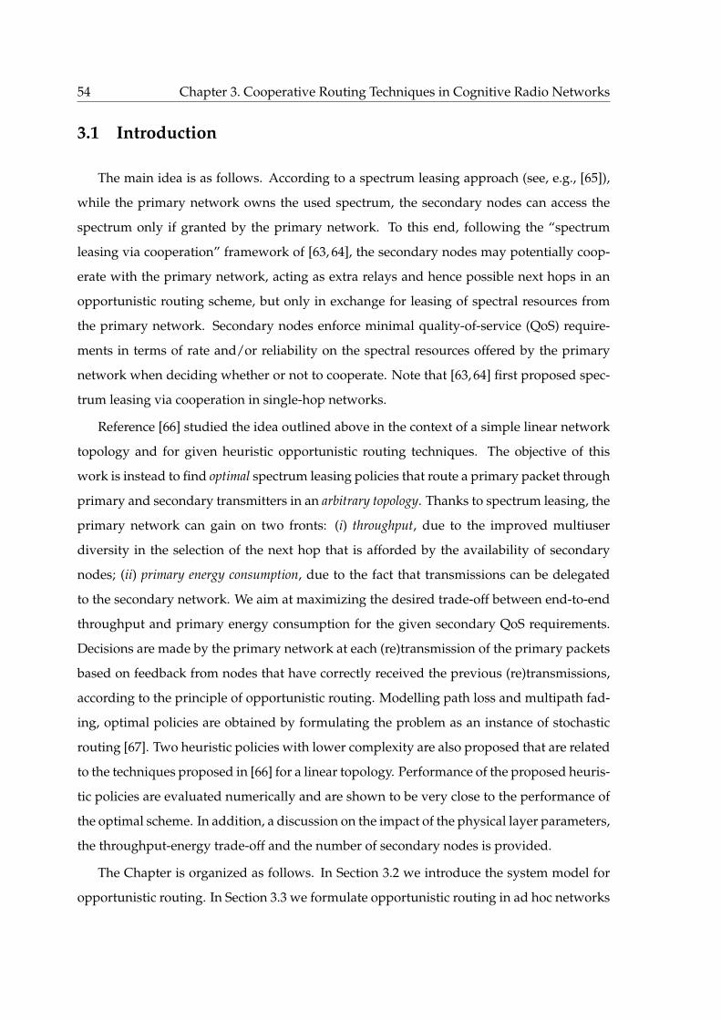
54 Chapter 3. Cooperative Routing Techniques in Cognitive Radio Networks
3.1 Introduction
The main idea is as follows. According to a spectrum leasing approach (see, e.g., [65]),
while the primary network owns the used spectrum, the secondary nodes can access the
spectrum only if granted by the primary network. To this end, following the “spectrum
leasing via cooperation” framework of [63, 64], the secondary nodes may potentially coop-
erate with the primary network, acting as extra relays and hence possible next hops in an
opportunistic routing scheme, but only in exchange for leasing of spectral resources from
the primary network. Secondary nodes enforce minimal quality-of-service (QoS) require-
ments in terms of rate and/or reliability on the spectral resources offered by the primary
network when deciding whether or not to cooperate. Note that [63, 64] first proposed spec-
trum leasing via cooperation in single-hop networks.
Reference [66] studied the idea outlined above in the context of a simple linear network
topology and for given heuristic opportunistic routing techniques. The objective of this
work is instead to find optimal spectrum leasing policies that route a primary packet through
primary and secondary transmitters in an arbitrary topology. Thanks to spectrum leasing, the
primary network can gain on two fronts: (i) throughput, due to the improved multiuser
diversity in the selection of the next hop that is afforded by the availability of secondary
nodes; (ii) primary energy consumption, due to the fact that transmissions can be delegated
to the secondary network. We aim at maximizing the desired trade-off between end-to-end
throughput and primary energy consumption for the given secondary QoS requirements.
Decisions are made by the primary network at each (re)transmission of the primary packets
based on feedback from nodes that have correctly received the previous (re)transmissions,
according to the principle of opportunistic routing. Modelling path loss and multipath fad-
ing, optimal policies are obtained by formulating the problem as an instance of stochastic
routing [67]. Two heuristic policies with lower complexity are also proposed that are related
to the techniques proposed in [66] for a linear topology. Performance of the proposed heuris-
tic policies are evaluated numerically and are shown to be very close to the performance of
the optimal scheme. In addition, a discussion on the impact of the physical layer parameters,
the throughput-energy trade-off and the number of secondary nodes is provided.
The Chapter is organized as follows. In Section 3.2 we introduce the system model for
opportunistic routing. In Section 3.3 we formulate opportunistic routing in ad hoc networks

3.2. System model 55
Po Pd
Figure 3.1. A possible representation of a primary distributed network (white circles) with NP = 7 relay
nodes and a secondary network (grey circles) with NS = 6 relay nodes.
with arbitrary topology as a stochastic routing problem [67]. In Section 3.4 we devise dis-
tributed heuristic routing schemes, which are thus numerically compared against optimal
routing in Section 3.5. Our concluding remarks are given in Section 3.6.
3.2 System model
A packet from a primary source Po is to be routed to the primary destination Pd through
two sets of relays. The first set RP is formed by NP primary nodes, while the second set RS
consists of NS secondary nodes that coexist with the primary network via spectrum leasing.
Specifically, as detailed below, a secondary relay can transmit only if leased a portion of the
spectrum by the primary network. The two sets of relays are arbitrarily placed in a square
area with normalized side equal to one, where source Po and destination Pd are positioned in
the middle of two opposite sides (see Fig. 3.1). The position of each node is static and known
by the all nodes in the network. Define the set of all nodes as T = RP ∪RS ∪ Po, Pd.
Time is slotted and all nodes work in half-duplex mode, so they cannot transmit and
receive simultaneously. In each block only one node is active, so that no spatial reuse is al-

56 Chapter 3. Cooperative Routing Techniques in Cognitive Radio Networks
lowed, and the transmission is composed of l (complex) channel uses.1 In the first block, the
primary packet of lRP bits is trasmitted by the primary source Po, where RP is the transmis-
sion rate of the licensed transmission in bits/s/Hz. In the following blocks, retransmissions
may be done by the source Po or by one of the relays, either primary or secondary, until the
final primary destination Pd correctly receives the packet. Retransmissions are done accord-
ing to a Type-I HARQ process: error correction coding is used, but previous undecodable
transmissions are discarded and detection is only based on the current transmission. After
correct decoding, the process starts again with a trasmission of a new primary packet by the
primary source Po. Notice that this implies that the source is always backlogged.
Routing decisions are made in an on-line manner by the primary network, which chooses
the next hop based on the feedback received at the end of the previous block from all nodes,
primary and secondary, that have successfully received the packet. The mechanism used
by the relays to send acknowledgements to the primary network is not further analyzed
here. In practice, decision may be made at the current transmitter if appropriate control of
secondary nodes by the primary network is enforced. A study on the design of feedback
signalling can be found in [69, 70] for systems with no secondary nodes.
When routing, the primary network is aware that any secondary node is willing to coop-
erate with the primary network, by acting as relay for the current primary packet, but only
under the condition that the primary network leases sufficient resources for transmission of
secondary traffic. In particular, if granted transmission, a secondary node multiplexes the
primary packet with a secondary packet. This principle was referred to as spectrum leasing
via cooperation and first proposed in [63,64] (see Section 3.1). Multiplexing is here done using
superposition coding (SC), see, e.g., [71]: the primary packet is summed to the secondary
packet with an appropriate power allocation 0 ≤ ψ ≤ 1 and then transmitted. The fraction ψ
is set so as to satisfy the desired secondary QoS requirements in terms of rate and reliability.
In particular, we assume that each secondary node requires for its own traffic transmitted
at rate RS to a node at distance dS, an outage probability of at most ǫS. This will be further
discussed below. We finally remark that optimality of SC in a Gaussian broadcast is well
known [71] and was extended to the scenario at hand in [72].
1In the absence of bandwidth expansion, l complex channel uses over a bandwidth of W Hz amount to l/W
s (see, e.g. [68]).

3.2. System model 57
3.2.1 Signal Model and Outage Probabilities
Considering a transmission from node a ∈ T r Pd, let ya,n(b, t) denote the discrete-
time (complex) baseband sample received by the node n ∈ T r Po during the b-th block
at channel use t, t = 1, . . . , l. The channel between nodes a and n is denoted as ha,n(b) and
assumed to be constant within a block (block-fading), Rayleigh distributed with zero mean
and unit power. Moreover, notation xa(b, t) represents the discrete-time (complex) baseband
sample transmitted by the scheduled node a with a per-symbol power constraint fixed to
E[|xa(b, t)|
2]≤ EN, t = 1, . . . , l, where EN is equal to EP or ES when the transmitter is a
primary or a secondary node, respectively. The relation between transmitter and receiver is
given by
ya,n(b, t) = d−η/2a,n ha,n(b)xa(b, t) + za,n(b, t), (3.1)
where da,n is the distance between the nodes, η is the power path-loss exponent and za,n(b, t)
represents the complex white Gaussian noise term with zero mean and power E[|za,n(b, t)|2] =
N0.
Channel state information ha,n(b) is not known to the transmitter node a, but only to the
receiver node n. The signal-to-noise ratio (SNR) for primary users is given by ξP = EP/N0
denoting the ratio between the maximum average energy directly received by Pd from the
source Po and the noise power N0. Hence, the term ξPd−η represents the average SNR for
a transmission from a primary node that covers a distance d. For completeness, ξSd−η =
ES/N0d−η denotes the average SNR for a transmission from a secondary node that covers a
distance d.
We now detail the outage probabilities and we discuss the secondary QoS requirements,
which are parametrized by the parameterQ, which represents the tuple (dS, RS, ǫS) or equiv-
alently the parameter ψ. First, consider the transmission from a primary node a ∈ RP∪Po.
Let Pout,P(da,n) be the outage probability for a packet transmitted by the primary node a to
a primary or secondary node n ∈ T r Po at distance da,n. Assuming that the coding block
is long enough, we have (see, e.g., [68]),
Pout,P(da,n) = Prlog2
(1 + |ha,n|
2ξPd−ηa,n
)≤ RP
= 1− exp
(−2RP − 1
ξPd−ηa,n
). (3.2)

58 Chapter 3. Cooperative Routing Techniques in Cognitive Radio Networks
Now consider the transmission from a secondary node. As explained above, this com-
bines both primary and secondary data using SC. Moreover, the power allocation parameter
ψ must be designed so as to meet the QoS requirements of the secondary users. In order to
decode either the primary or the secondary packet, receivers at all nodes employ two de-
coders in parallel so that detection of the desired message is correct if either one of the two
decoders decodes correctly. The first decoder decodes the desired packet (primary or sec-
ondary) by treating the undesired packet as additive Gaussian noise. The second decoder,
instead, estimates and cancels the undesired packet from the received signal and then de-
codes the desired packet from the interference-free signal. Based on this discussion, the out-
age probability for decoding of a primary packet transmitted by the secondary node a ∈ RS
to a primary or secondary node n ∈ T rPo at distance da,n is given by (see for details [72])
Pout,SP(da,n) = 1− exp[−min
(H
(1)P ,H
(2)P
)], (3.3)
where the threshold H(1)P represents the outage probability of the first decoder, in which
the interference (i.e., secondary packet) is treated as noise. The remaining term H(2)P is the
outage probability of the successive decoding scheme, where the receiver first decodes the
secondary packet and then the primary one. These thresholds can be evaluated as
H(1)P =
∞, 0 ≤ ψ ≤ 1− 2−RP
2RP−1(1−(1−ψ)2RP )ξSd
−ηa,n, 1− 2−RP < ψ ≤ 1
(3.4)
H(2)P =
max
2RS−1
(1−ψ2RS )ξSd−ηa,n, 2RP−1ψξSd
−ηa,n
, 0 < ψ < 2−RS
∞, ψ = 0 and 2−RS ≤ ψ ≤ 1. (3.5)
The choice of ψ depends, as discussed above, on the secondary QoS requirements (dS, RS,
ǫS). So, similarly to (3.3), we need the expression of the outage probability that a secondary
packet (superimposed with a primary message) transmitted by a secondary node is not
decoded correctly by a secondary node placed at distance d. This term is given by
Pout,SS(d) = 1− exp[−min
(H
(1)S ,H
(2)S
)], (3.6)
whereH(1)S andH(2)
S are
H(1)S =
2RS−1(1−ψ2RS )ξSd−η , 0 ≤ ψ < 2−RS
∞, 2−RS ≤ ψ ≤ 1, (3.7)

3.3. Optimal Routing Policies 59
and
H(2)S =
∞, 0 ≤ ψ ≤ 1− 2−RP and ψ = 1
max
2RP−1(1−(1−ψ)2RP )ξSd−η ,
2RS−1(1−ψ)ξSd−η
, 1− 2−RP < ψ < 1
. (3.8)
Recalling that a fraction 1−ψ of the transmitted power is used for the secondary’s own traffic
and imposing the condition on the outage probability as Pout,SS(dS) = ǫS, we can numerically
extract the parameter ψ from this equation for a given rate pair (RP,RS).
3.2.2 Performance Metrics
Thanks to spectrum leasing, the primary network can gain on two fronts: 1) through-
put, because of an improved multiuser diversity in the selection of the next hop, due to
the availability of secondary nodes; 2) primary energy consumption, due to the fact that
transmissions can be delegated to the secondary network.
We define the primary end-to-end throughput T (k,RP,Q) as the average number of suc-
cessfully transmitted bits per second per Hz, given the total number of hops k, the primary
transmission rate RP and the tupleQ. Using renewal theory, the throughput is given as (see,
e.g., [73]):
T (k,RP,Q) =RP
E[M ], (3.9)
where M is the total number of time slots used to correctly forward a given primary packet
from the source Po to the destination Pd, i.e., M = MP +MS where MP and MS represent
the number of primary and secondary transmissions, respectively. We also define the primary
energy E(k,RP,Q) as the average overall energy spent by the primary network to deliver a
packet successfully, normalized with respect to the energy expenditure of a single primary
transmission. Therefore, this quantity is measured via the number of time slots that involve
primary transmissions,
E(k,RP,Q) = E[MP]. (3.10)
3.3 Optimal Routing Policies
The problem to be solved is to find optimal routing transmission policies for the sce-
nario discussed above. With the term optimal we refer here to policies that minimize, across
all the possible evolutions of the system, the expected throughput (throughput optimal), the

60 Chapter 3. Cooperative Routing Techniques in Cognitive Radio Networks
expected total transmission energy expended by primary users (energy optimal) or a combi-
nation of throughput and primary energy through a weighting factor α ∈ [0, 1]. We show
below that the problem can be formulated as an instance of stochastic routing [67].
Time is slotted and a single copy of the packet is transmitted in any slot k = 0, 1, 2, 3, . . . .
The system evolution is described through a suitable Markov chain with states xk ∈ Ω,
where Ω is the set of all states and xk ⊆ T identifies the nodes that have correctly decoded
the packet up to and including time slot k. Moreover, we define the starting state s as the
state in which only the primary source has the packet and the final state f , state in which the
primary destination has been reached.
At time k = 0, only the primary source Po has the packet and the Markov chain is in state
s (i.e., x0 = s). In the first transmission slot, k = 1, Po transmits its packet and the system
moves to x1 ⊇ s. If Pd /∈ x1, a relay node a ∈ x1 (either primary or secondary) is selected
from x1 to transmit the packet in the next time slot k = 2. This process is iterated for the
subsequent slots k = 3, 4, . . . , until the destination node Pd correctly receives the packet, i.e.,
Pd ∈ xk. At this point, the Markov chain transitions to the final state f with probability one
and the cost associated with this transition is zero.
The dynamics of the network are captured by transition probabilities pxy(a), x, y ∈ Ω,
with y ⊇ x and a ∈ x, which return the probability that, starting from state x, the system
transitions to state y, that is, nodes in y \ x correctly receive the packet, when node (ac-
tion) a is elected as the relay. For the computation of pxy(a), we define the outage probability
pout(a, n) for any node n ∈ T when a is the transmitter and da,n is their distance:
pout(a, n) =
Pout,P(da,n) when a ∈ RP ∪ Po
Pout,SP(da,n) when a ∈ RS .(3.11)
Moreover, for x 6= f with Pd /∈ x and y 6= f , we define
Pxy(a) =∏
n∈T s.t.n∈y,n/∈x
[1− pout(a, n)]∏
m∈T s.t.m/∈y
pout(a,m) . (3.12)

3.3. Optimal Routing Policies 61
Thus, it follows that
pxy(a) =
0 (Pd ∈ x or x = f) and y 6= f
1 (Pd ∈ x or x = f) and y = f
0 Pd /∈ x, x 6= f and y = f
Pxy(a) Pd /∈ x, x 6= f and y 6= f
(3.13)
The final state f is absorbing, i.e., pff (a) = 1, ∀ a ∈ f .
Each transition also has an associated cost c(x, a, y) and the goal is to minimize the total
expected discounted cost
J(s)def= Eπ
[+∞∑
k=0
γkc(x, a, y)
∣∣∣∣x0 = s
], (3.14)
where γ ∈ (0, 1) is a discount factor and Eπ[·|x0 = s] is the conditional expectation given
that routing policy π is employed. The cost c(x, a, y) is incurred when the current state is
x ∈ Ω, action a ∈ x is selected and the system moves to state y ∈ Ω. In detail, we have
c(x, a, y) = αcThr(x, a, y) + (1− α)cE(x, a, y) , (3.15)
where cThr(x, a, y) accounts for the throughput cost, cE(x, a, y) is the energy cost for the pri-
mary users involved in the transmission process and α ∈ [0, 1] is a weighting factor.
The cost functions in (3.15) are defined as follows. For the throughput cost we set
cThr(x, a, y) = 1, ∀x, y ∈ Ω, a ∈ x so that the total accumulated throughput cost equals
the number of transmissions performed to correctly deliver a data packet from Po to Pd.
Due to (3.9), minimizing cThr is equivalent to maximizing the end-to-end throughput.
For the energy cost we have,
cE(x, a, y) =
1 when a ∈ RP ∪ Po
0 when a ∈ RS .(3.16)
Thus, cE(x, a, y) accounts for the number of primary transmissions associated with the tran-
sition from x to y, so that the accumulated energy cost represents the total number of pri-
mary transmissions MP incurred in correctly delivering a packet from Po to Pd. Hence, due
to (3.10) minimizing the energy cost cE(x, a, y) amounts to minimizing the total primary
energy expenditure to correctly deliver a packet from the source Po to the destination Pd.

62 Chapter 3. Cooperative Routing Techniques in Cognitive Radio Networks
Using the definitions above, the problem is an instance of the stochastic routing problem
defined in [67]. Thus, an optimal policy in the form of an index policy for the considered
problem is guaranteed to exist and can be found using the algorithms provided in [67].
In [67], both a centralized and a distributed implementation are provided. The centralized
implementation has a complexity of O(|T |2), requires full knowledge of the network topol-
ogy and can be used to obtain offline, optimal index policies. In particular, the centralized
algorithm determines a global ranking of the nodes of the network that can be used at each
hop to determine the best relay node. The distributed implementation computes the optimal
index policies in a distributed fashion through the repeated exchange of local information
among neighboring nodes. The convergence time of the distributed implementation de-
pends on the particular network topology and thus cannot be inferred a priori.
3.4 Heuristic Routing Policies
In this section, we detail two low-complexity heuristic policies that adopt the spectrum
leasing via opportunistic routing technique and are suitable for a distributed implementa-
tion. With these policies the relay selection is made on the fly by the current transmitter
at each hop, only based on local interactions. The optimal policies of Section 3.3, instead,
are determined either through a centralized solver that requires full knowledge of the net-
work topology and are then used in an offline manner, or through a distributed computation
which requires an iterative exchange of messages among neighboring nodes in order to con-
verge to the optimal solution.
We introduce a primary energy budget K which permits to control the trade-off between
the primary energy consumption and the end-to-end throughput. In particular, K repre-
sents the maximum number of primary relays that can be used to route any given primary
packet from Po to Pd (note that K does not take into account the retransmissions performed
by these nodes). We considered this definition of K for analytical simplicity and to reduce
complexity.
The primary energy budget K is stored within the packet header and decremented by
one unit each time a new primary relay is selected. At each time slot k = 0, 1, . . . , we have
K = Kused +Kres, where Kused is the number of primary relays already used in the current
routing path. If the residual energy budget Kres > 0 then the next relay can either be a

3.4. Heuristic Routing Policies 63
primary or a secondary node. Otherwise, if Kres = 0, the current primary transmitter is the
last primary node that can be used along the routing path from Po to Pd. Subsequent relays
must all be secondary nodes.
Observe that using the energy budgetK has the potential drawback of limiting the avail-
able multiuser diversity, as fewer receivers will be available to act as relay, and thus reducing
the achievable end-to-end throughput. Moreover, secondary users only allocate a portion
ψ of the total power for their primary transmissions, so that they can cover a shorter dis-
tance with respect to primary transmissions for the same outage probability (assuming they
use the same transmitting power). We now detail two heuristic routing policies for primary
packets.
3.4.1 K-Closer
The K-Closer policy aims at minimizing the overall number of network transmissions
while controlling the energy consumption of primary users through the budget parameter
K. Let us consider a generic transmitter at time slot k, which broadcasts a copy of the
primary packet. All nodes that correctly receive it are ranked by the transmitter according
to their distance from the destination Pd so that closer nodes have a higher rank.2 Now, if
Kres > 0, the transmitter elects as the relay the receiver with the highest rank; if this receiver
is a primary node, Kres is decremented by one while it is left unchanged otherwise. On the
other hand, if Kres = 0, the transmitter elects as the relay the secondary node having the
highest rank. This process is iterated until the primary packet is correctly received by Pd.
3.4.2 K-One Step Look Ahead (K-OSLA)
The potential drawback of K-Closer is to choose, due to the limited amount of informa-
tion that it uses, a relay with a small number of neighbors in its proximity. Notably, this
leads to an increase in the average number of retransmissions that are necessary to reach the
next relay. In what follows, we extend the K-Closer heuristic to avoid this situation.
For any node a ∈ RP ∪RS let δa = da,Pd, denote the proximity of a to the destination Pd.
We assume that each node a can collect this proximity metric from all nodes (both primary
2This implies a feedback mechanism from the receivers to the transmitter, whose design is out of the scope
of this work.

64 Chapter 3. Cooperative Routing Techniques in Cognitive Radio Networks
and secondary) that are closer to the destination with respect to itself. After that, a builds an
ordered set B(a) as follows: B(a) =n1, n2, . . . , n|B(a)|
, where ni ∈ T rPo and δa ≥ δni ≥
δni+1 , i = 1, . . . , |B(a)| − 1. At the same time, node a determines the ordered subset BS(a) ⊆
B(a), with BS(a) =m1,m2, . . . ,m|BS(a)|
, which only contains the secondary nodes in
B(a). This procedure is carried out for each node a ∈ RP ∪RS , except the destination Pd.
Also, let ga,n = δa−δn denote the geographical advancement of a toward Pd provided
by a relay node n. Moreover, we define the expected geographical advancement toward the
destination provided by node awhen both primary and secondary nodes can act as relay as:
ga =
|B(a)|∑
i=1
ga,ni [1− pout(a, ni)]
|B(a)|∏
j=i+1
pout(a, nj) . (3.17)
Similarly, we define gSa as the expected geographical advancement toward the destination
given by node a when only secondary nodes can be selected as relay, i.e.,
gSa =
|BS(a)|∑
i=1
ga,mi [1− pout(a,mi)]
|BS(a)|∏
j=i+1
pout(a,mj) . (3.18)
Finally, we introduce Ga,n = ga,n + gn that represents the overall expected advancement,
with respect to a, provided in the next two transmission hops by the selection of node n.
Similarly defined is GSa,n = ga,n + gSn .
K-OSLA works as follows. Let a be the node that sends the primary packet and r1, . . . , rM
be the M nodes that successfully decoded it. If Kres > 1, the transmitter a rearranges this
set according to the metrics Ga,r1 , . . . , Ga,rM and selects as the relay the receiver node
r∗ ∈ r1, . . . , rM with the highest metric Ga,r∗ (i.e., Ga,r∗ ≥ Ga,ri ∀ i = 1, . . . ,M ). If r∗ is a
primary user, Kres is decremented by one. When Kres = 1, the transmitter a orders the set
r1, . . . , rM using the metric GSa,ri or Ga,ri in case that ri is a primary or a secondary node,
respectively, with i = 1, . . . ,M . Afterwards, the transmitter a selects as relay the receiver
node with the highest metric, and if it is a primary user, Kres is decremented by one. Finally,
if Kres = 0, only secondary nodes of the set r1, . . . , rM are ranked according to the metric
GSa,n and the secondary node having the highest metric is selected by the transmitter as the
next relay. This procedure is iterated until the packet is correctly received by Pd.

3.5. Numerical results 65
3.5 Numerical results
In this section we present the performance of optimal and heuristic routing in the dis-
cussed opportunistic network with spectrum leasing.
For the results in this section we assume the following. We consider a random network
with one source Po, one destination Pd, NP = 8 primary nodes, an equal transmitting power
for primary and secondary users, i.e. EP = ES, which yields ξP = ξS = ξ, where we set
ξ = −5 dB. Relay nodes are uniformly placed at random in a square area with normalized
side equal to one, where source Po and destination Pd are positioned in the middle of two
opposite sides. Optimal policies are obtained setting γ = 0.99, which is adequate for static
networks. For the QoS of the secondary network we consider the following. The fraction
of power allocated to primary transmissions ψ is computed by imposing an outage proba-
bility of ǫS = 0.1 for the transmission for a secondary packet, at rate RS, between any two
secondary nodes placed at a distance dS = 0.1. From (3.6) we see that the ψ satisfying these
QoS requirements is not necessarily unique but it rather depends on the type of decoding
technique used at the receiver(s). In the following results, we always select the value of
ψ that maximizes the primary throughput, i.e., the highest ψ. As performance criteria, we
plot the performance of the considered routing schemes in terms of primary end-to-end
throughput (3.9) vs primary energy consumption (expressed in dB, i.e., 10 log10E(k,RP,Q),
see (3.10)).
In Fig. 3.2 we set RP = 3 bits/s/Hz, RS = 1 bits/s/Hz and NS = 8. The points in
this figure have been obtained by varying α in [0, 1] for the optimal policy (Optimal) and K
in 0, . . . , NS for the heuristic policies (K-Closer and K-OSLA). The performance of op-
timal and heuristic policies when spectrum leasing is not used (indicated in the figure as
“No SL”) is also shown for comparison. We observe that cooperation via spectrum leasing
allows for improved performance in terms of throughput and energy. Both K-Closer and
K-OSLA for increasing K provide better throughput performance at the cost of a slightly
increased primary energy consumption. This is due to the fact that larger values of K en-
able the selection of a large number of primary relay nodes. As expected,K-OSLA improves
over K-Closer in terms of throughput performance, especially for high values of K (K ≥ 3
in the figure). In fact, for increasing K the multiuser diversity is higher as more primary
nodes can be selected along the path from Po to Pd. Note that, as we discuss below, see

66 Chapter 3. Cooperative Routing Techniques in Cognitive Radio Networks
K = 0
K = 8
α = 0
α = 1
0.1
0.2
0.3
0.4
0.5
0.6
0 2 4 6 8 10 12
Th
rou
gh
pu
t [b
its/
s/H
z]
Primary Energy [dB]
OptimalK-OSLAK-Closer
Optimal, No SLK-OSLA, No SLK-Closer, No SL
Figure 3.2. End-to-end throughput vs overall primary energy plotted varying α ∈ [0, 1] for the optimal
policy (solid line) and K ∈ 0, . . . , NS for the heuristic policies (dotted lines). The results are obtained
for NP = NS = 8, ξ = −5 dB, RP = 3 bits/s/Hz and RS = 1 bits/s/Hz.
Fig. 3.5, the throughput increase of K-OSLA can even be much larger than the one obtained
in Fig. 3.2 if we increase RS (i.e., the secondary QoS requirements). For the primary energy
consumption, as expected, for K = 0 (i.e., the relays are all secondary nodes) the energy ex-
penditure of the two schemes is the same. Instead, for K ≥ 1, K-OSLA has a slightly higher
energy consumption with respect to K-Closer and this is due to the fact that the expected
advancement metric slightly favors primary nodes. In fact, these nodes provide higher ex-
pected advancements due to the higher transmission power they use for the transmission of
primary packets.
With Fig. 3.3 we investigate how close heuristic policies can get to the optimal through-
put performance (α = 1). The curves in this figure have been obtained setting K = 8
and varying the number of secondary nodes NS ∈ 0, 2, 4, 6, 8, 12. The main observations
from this plot are that: 1) the usage of spectrum leasing allows for a substantial increase in
the throughput (twofold increase) and primary energy performance (gains as high as 6 dB)
with respect to the case where only primary transmissions are allowed (i.e., NS = 0) and 2)
K-OSLA approaches the optimal throughput performance for nearly all values of NS .
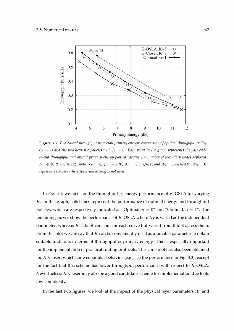
3.5. Numerical results 67
NS = 0
NS = 12
0.1
0.2
0.3
0.4
0.5
0.6
4 5 6 7 8 9 10 11 12
Th
rou
gh
pu
t [b
its/
s/H
z]
Primary Energy [dB]
K-OSLA, K=8K-Closer, K=8Optimal, !=1
Figure 3.3. End-to-end throughput vs overall primary energy: comparison of optimal throughput policy
(α = 1) and the two heuristic policies with K = 8. Each point in the graph represents the pair end-
to-end throughput and overall primary energy plotted varying the number of secondary nodes deployed
NS ∈ 0, 2, 4, 6, 8, 12, with NP = 8, ξ = −5 dB, RP = 3 bits/s/Hz and RS = 1 bits/s/Hz. NS = 0
represents the case where spectrum leasing is not used.
In Fig. 3.4, we focus on the throughput vs energy performance of K-OSLA for varying
K. In this graph, solid lines represent the performance of optimal energy and throughput
policies, which are respectively indicated as “Optimal, α = 0” and “Optimal, α = 1”. The
remaining curves show the performance of K-OSLA where NS is varied as the independent
parameter, whereas K is kept constant for each curve but varied from 0 to 8 across them.
From this plot we can say that K can be conveniently used as a tunable parameter to obtain
suitable trade-offs in terms of throughput vs primary energy. This is especially important
for the implementation of practical routing protocols. The same plot has also been obtained
for K-Closer, which showed similar behavior (e.g., see the performance in Fig. 3.3), except
for the fact that this scheme has lower throughput performance with respect to K-OSLA.
Nevertheless, K-Closer may also be a good candidate scheme for implementation due to its
low complexity.
In the last two figures, we look at the impact of the physical layer parameters RP and

68 Chapter 3. Cooperative Routing Techniques in Cognitive Radio Networks
NS = 2
NS = 12
K = 0
K = 8
0.1
0.2
0.3
0.4
0.5
0.6
0 2 4 6 8 10 12
Th
rou
gh
pu
t [b
its/
s/H
z]
Primary Energy [dB]
Optimal, ! = 0Optimal, ! = 1
K-OSLA
Figure 3.4. Impact of K on the heuristic policy K-OSLA by varying the number of secondary nodes
deployed NS ∈ 2, 4, 6, 8, 12, with NP = 8, ξ = −5 dB, RP = 3 bits/s/Hz and RS = 1 bits/s/Hz. The
performance of the optimal routing policy is also shown by varying NS ∈ 2, 4, 6, 8, 12 for α = 0 (energy
optimal) and α = 1 (throughput optimal).
the QoS requirements of secondary users, expressed through RS, considering α = 1 for the
optimal routing policy andK = 8 for the heuristic policies (so as to maximize their through-
put performance). Fig. 3.5 is obtained for a fixed number of secondary nodes NS = 8,
RP = 3 bits/s/Hz and varying the secondary transmission rate RS ∈ 0.5, 1.5, 2.5, 3.5, 4.5
bits/s/Hz. First of all, for increasing RS the primary throughput decreases, up to a certain
point, for all schemes. This is because an increasing RS leads to a smaller coverage for the
secondary transmissions, which means that more secondary transmissions (and secondary
relays) are needed to reach Pd. However, when RS gets too high (i.e., RS ≥ 2.5 bits/s/Hz in
the figure) the secondary nodes are no longer used as relays because the portion of power
ψ that they allocate to primary transmissions is too small to allow the correct reception, at
any node, of the primary packets they send. Hence, more and more primary nodes are used
and the end-to-end throughput increases. For this same reason, the primary energy always
increases for increasing RS. The latter aspects are emphasized by K-OSLA: this scheme
obtains a much higher throughput at the cost of a higher primary energy consumption,

3.5. Numerical results 69
RS = 0.5
RS = 4.5
0.1
0.2
0.3
0.4
0.5
0.6
4 5 6 7 8 9 10 11 12
Th
rou
gh
pu
t [b
its/
s/H
z]
Primary Energy [dB]
K-OSLA, K=8K-Closer, K=8Optimal, !=1
Optimal, No SL
Figure 3.5. End-to-end throughput vs overall primary energy plotted varying RS for the throughput
optimal policy (α = 1) and for the heuristic policies with K = 8, NP = 8, ξ = −5 dB and RP = 3
bits/s/Hz. The curves are obtained by varying RS ∈ 0.5, 1.5, 2.5, 3.5, 4.5 bits/s/Hz.
especially when RS is high. In fact, with respect to K-Closer, K-OSLA uses the expected
advancement metric which selects with higher probability a primary node as the next relay
(the expected advancement of secondary nodes is smaller than that of primary users). Fi-
nally, we note that, for the considered value of RS,K-OSLA outperforms the optimal routing
policy with no spectrum leasing (here referred to as “No SL”), providing better throughput
as well as energy performance.
In Fig. 3.6, we analyze the impact on the throughput/energy performance of the trans-
mission rate RP ∈ 0.5, 1.5, 2.5, 3.5, 4.5 bits/s/Hz for RS = 1 bits/s/Hz. From this plot
we see that there exists a primary rate, R*P, that maximizes the throughput. For example,
R*P = 1.5 bits/s/Hz for No SL and R*
P = 2.5 bits/s/Hz for the other schemes. Also in
this case, the gains of K-Closer and K-OSLA over No SL are substantial, irrespective of the
value of RP. As a final remark, for all policies the primary energy consumption can be re-
duced through a reduction of the transmission rate RP and this is due to the corresponding
larger coverage range offered by the relay nodes.

70 Chapter 3. Cooperative Routing Techniques in Cognitive Radio Networks
RP = 0.5
RP = 4.5 0.1
0.2
0.3
0.4
0.5
0.6
0 2 4 6 8 10 12 14 16 18
Th
rou
gh
pu
t [b
its/
s/H
z]
Primary Energy [dB]
K-OSLA, K=8K-Closer, K=8Optimal, !=1
Optimal, No SL
Figure 3.6. End-to-end throughput vs overall primary energy plotted varying RP for the throughput
optimal policy (α = 1) and for the heuristic policies with K = 8, NP = 8, ξ = −5 dB and RS = 1
bits/s/Hz. The curves are obtained by varying RP ∈ 0.5, 1.5, 2.5, 3.5, 4.5 bits/s/Hz.
3.6 Conclusions
Design of routing protocols in cognitive radio multihop networks, where primary and
secondary nodes coexist over the same spectral resource, is made difficult by the conflicting
requirements of the two classes of nodes. In this Chapter, a spectrum leasing solution to this
problem is proposed, wherein secondary nodes are granted the possibility to transmit by the
primary network in exchange for forwarding primary packets. The primary network goal is
maximizing an appropriate trade-off between throughput and energy gains that are accrued
by the cooperation of secondary networks, whereas secondary nodes enforce minimum QoS
requirements when deciding whether or not to cooperate. Routing decisions are made by
the primary network in an on-line fashion according to the principle of opportunistic routing
based on the secondary QoS requirements. We refer to this strategy as spectrum leasing via
cooperative opportunistic routing. Optimization of the strategy is tackled by framing the
routing design as a stochastic routing problem. Two heuristic policies with lower complexity
are also proposed. Our numerical results lend evidence to the throughput and energy gains

3.6. Conclusions 71
that can be attained by the proposed spectrum leasing approach by the primary network,
all the while allowing also the secondary nodes to transmit. Moreover, the heuristic policies
are shown to provide flexible solutions that perform close to the optimal policy.


Chapter 4Distributed Data Gathering in Wireless
Sensor Networks
Wireless sensor networks have found applications in a large number of fields such as en-
vironmental sensing and structural health monitoring [74]. In such applications, the main-
tenance necessary to replace the batteries when depleted is often of prohibitive complexity,
if not impossible. Therefore, sensors that harvest energy from the environment, e.g., in the
form of solar, thermal, vibrational or radio energy [75] [76], have been proposed and are
now commercially available.
Given the interest outlined above, the problem of designing optimal transmission pro-
tocols for energy harvesting wireless sensor networks has received considerable attention.
Specifically, reference [77] presents cross-layer resource allocation algorithms for wireless
networks operating with rechargeable batteries, under general arrival, channel state and
recharge processes. The algorithms proposed in [77] aim at maximizing a total system util-
ity while satisfying energy and power constraints, and they are shown to achieve close-to-
optimal performance. [78] designs a routing scheme to optimally utilize the available energy
in multihop radio networks in the presence of energy constraints, and it is shown to perform
asymptotically optimal with respect to the number of nodes in the network. The proposed
algorithm assumes no statistical information on packet arrivals and is suitable for a dis-
tributed implementation. [79] uses a Lyapunov optimization approach for algorithm design
to achieve close-to-optimal utility performance in energy harvesting networks with finite
capacity energy storage devices. Moreover, [79] proposes the novel idea of perturbation-

74 Chapter 4. Distributed Data Gathering in Wireless Sensor Networks
based Lyapunov optimization, which allows to develop algorithms that take actions with
the objective of pushing the energy levels towards certain nonzero values to avoid energy
outage, without complicating their performance analysis. Without considering energy har-
vesting, [80] presents a static routing scheme which aim at maximizing the lifetime of a
network with finite energy capacity. The solution exploits the knowledge of the traffic pat-
terns and energy replenishment statistics, but does not use any instantaneous information
on node energy, and achieves a close-to-maximum lifetime when the energy claimed by each
packet is relatively small compared to the battery capacity.
The body of work reviewed above considers, as the only source of energy expenditure,
the energy used for transmission (e.g., the energy used by the power amplifiers). How-
ever, a distinguishing feature of sensor networks is that the sensors have not only transmis-
sion tasks, but also sensing and source coding tasks, such as compression, to be performed.
The source coding tasks entail a non-negligible energy consumption. In fact, reference [81]
demonstrates that the overall cost required for compression1 is comparable with that needed
for transmission, and that a joint design of the two tasks can lead to very significant energy
saving gains. Another distinguishing feature of sensor networks is that the sources measured
by different sensors are generally correlated.
The above mentioned trade-offs between energy used for compression, or more gener-
ally source coding, and transmission have been previously studied by [82] [83] in the frame-
work of Lyapunov optimization but without considering energy-harvesting or modeling
source correlation.
4.1 Introduction
In this Chapter, we focus on an energy-harvesting wireless sensor network by account-
ing for the energy costs of both source coding and transmission, and by modeling source
correlation. As for the latter, we assume that the sensors can perform distributed source
coding (see, e.g., [84]). This class of compression techniques enables sensors with correlated
measurements to trade, to an extent determined by the amount of correlation, the resources
used for source coding among them. In this way, for instance, a sensor that is running low
1This reference considers transmission of web data.

4.2. System model 75
on energy can benefit from the energy potentially available at a nearby node if the latter has
correlated measurements.
The use of distributed source coding techniques for multihop sensor networks has been
studied in [85] where the problem of optimizing the transmission and the compression strat-
egy was tackled under distortion constraints in a centralized fashion. Instead, [86] proposes
a distributed algorithm that maximizes an aggregate utility measure defined in terms of
the distortion levels of the sources. In this Chapter, following a formulation similar to [79],
we address a dynamic setting with time-varying sources and channels using the Lyapunov
optimization techniques developed in [87] [88], combined with the idea of weight pertur-
bation [79] [89]. We devise an efficient online algorithm that takes actions based only on
the instantaneous knowledge of the amount of harvestable energy, of the current channel
state and of the source state. We prove that the proposed policy is able to achieve an aver-
age network cost which can be made arbitrarily close to the optimal one with a controllable
trade-off with the sizes of the queues and the batteries.
The rest of the Chapter is organized as follows. In Section 4.2 we present the system
model and we state the optimization problem. In Section 4.3 we obtain a lower bound on
the optimal network cost for the proposed problem. In Section 4.4 we present our algorithm
designed following the Lyapunov optimization framework and we show how it can be im-
plemented in a distributed fashion. Section 4.5 formalizes the main results of our paper and
provide analytical insights into the performance of the proposed policy. Section 4.6 pro-
poses an extended version of the problem, in which the sink node acts as a cluster head and
is able to add some side information to improve the system performance. In Section 4.7 we
prove the effectiveness of our analytical analysis and discuss the impact of the optimization
parameters. Section 4.8 concludes the Chapter.
4.2 System model
We consider a wireless network modelled by a direct graph G = (N ∪ d,L), where
N = 1, 2, . . . , N is the set of nodes in the network, d is the destination (or sink), and
L ⊂ (n,m): n,m ∈ N ∪ d, n 6= m represents the set of communication links, see Fig. 4.1
for an illustration. We define lmax as the maximum degree that any node n ∈ N ∪ d can
have. As discussed below, we allow for fairly general interference models. We will consider
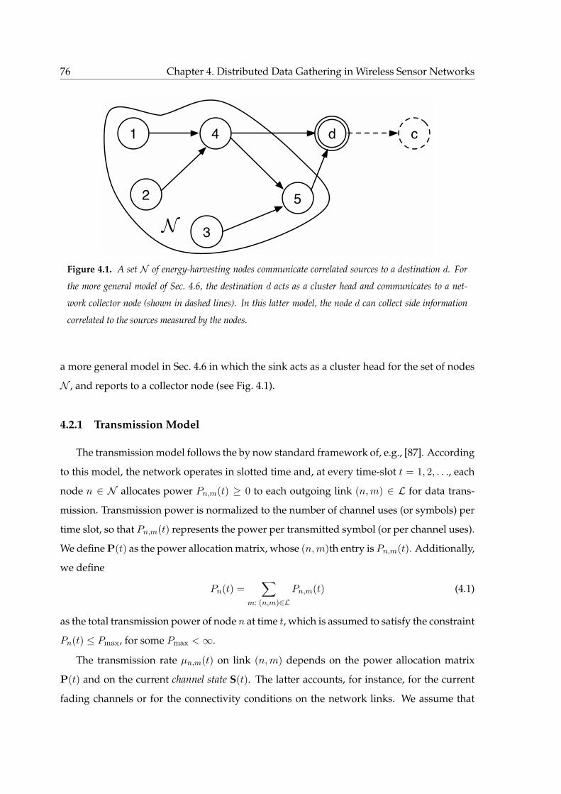
76 Chapter 4. Distributed Data Gathering in Wireless Sensor Networks
1 d
3
4
2 5
N
c
Figure 4.1. A set N of energy-harvesting nodes communicate correlated sources to a destination d. For
the more general model of Sec. 4.6, the destination d acts as a cluster head and communicates to a net-
work collector node (shown in dashed lines). In this latter model, the node d can collect side information
correlated to the sources measured by the nodes.
a more general model in Sec. 4.6 in which the sink acts as a cluster head for the set of nodes
N , and reports to a collector node (see Fig. 4.1).
4.2.1 Transmission Model
The transmission model follows the by now standard framework of, e.g., [87]. According
to this model, the network operates in slotted time and, at every time-slot t = 1, 2, . . ., each
node n ∈ N allocates power Pn,m(t) ≥ 0 to each outgoing link (n,m) ∈ L for data trans-
mission. Transmission power is normalized to the number of channel uses (or symbols) per
time slot, so that Pn,m(t) represents the power per transmitted symbol (or per channel uses).
We define P(t) as the power allocation matrix, whose (n,m)th entry is Pn,m(t). Additionally,
we define
Pn(t) =∑
m: (n,m)∈L
Pn,m(t) (4.1)
as the total transmission power of node n at time t, which is assumed to satisfy the constraint
Pn(t) ≤ Pmax, for some Pmax <∞.
The transmission rate µn,m(t) on link (n,m) depends on the power allocation matrix
P(t) and on the current channel state S(t). The latter accounts, for instance, for the current
fading channels or for the connectivity conditions on the network links. We assume that

4.2. System model 77
the channel state S(t) takes values in some finite set S = (s1, s2, . . . , sM ), and is constant
for the duration of a time-slot, but is independent and identically distributed (i.i.d.) across
time-slots. We use ρsi to denote the probability Pr [S(t) = si] for i = 1, . . . ,M . We write
µn,m(t) = Cn,m(P(t),S(t)), (4.2)
where Cn,m(P(t),S(t)) is the capacity-power curve for link (n,m) as measured in bits for
channel use. The latter depends on the specific network transmission strategy, which in-
cludes the modulation and coding/decoding schemes used on all links. We assume that
function Cn,m(P(t),S(t)) is continuous in P(t) and non decreasing in Pn,m(t). An example
of the function Cn,m(P(t),S(t)) is the Shannon capacity obtained by treating interference as
noise at the receivers, namely
Cn,m(P(t),S(t)) = log
(1 +
Pn,m(t)Sn,m(t)
N0 +∑
(l,n)∈L Pl(t)Sl,n(t)
), (4.3)
where channel state Sn,m(t) here represents the channel power gain on link (n,m) and N0 is
the noise spectral density. We assume that there exists some finite constant µmax such that
µn,m(t) ≤ µmax for all time t, any power allocation vector P(t) and channel state S(t). More-
over, following [79], we assume that the function Cn,m(P(t),S(t)) satisfies the following
properties:
Property 1: For any power allocation matrix P(t), we have:
Cn,m(P(t),S(t)) ≤ ξPn,m(t), (4.4)
for some finite constant ξ > 0;
Property 2: For any power allocation matrix P(t) and matrix P′(t) obtained by P(t) by
setting the entry Pn,m(t) to zero, we have:
Ca,b(P(t),S(t)) ≤ Ca,b(P′(t),S(t)), (4.5)
for all (a, b) ∈ L, with (a, b) 6= (n,m).
Note that both properties are satisfied by typical choices of function Cn,m(P(t),S(t))
such as (4.3). In fact, Property 1 is satisfied if function Cn,m(P(t),S(t)) is concave with respect
to Pn,m(t), while Property 2 states that interference due to power spent on other links cannot
be beneficial.2 Finally, we define the total outgoing transmission rate µn,∗(t) from a node2This may not be the case if sophisticated physical layer techniques are used, such as successive interference
cancelation (see, e.g., [90]).

78 Chapter 4. Distributed Data Gathering in Wireless Sensor Networks
n ∈ N at time t as
µn,∗(t) =∑
m: (n,m)∈L
µn,m(t), (4.6)
and the total incoming transmission rate µ∗,n(t) at a node n ∈ N as
µ∗,n(t) =∑
m: (m,n)∈L
µm,n(t). (4.7)
4.2.2 Data Acquisition, Compression and Distortion Model
At each time slot, each node of the network is able to sense the environment and to ac-
quire spatially correlated measurements. The measurements are then routed through the
network to be gathered by a sink node, as illustrated in Fig. 4.1. Before transmission, the
acquired data is compressed via adaptive lossy source coding by leveraging the spatial cor-
relation of the measurements. To elaborate, let O(t) denote the source state at time slot t.
This represent the joint distribution of the measurements, which are assumed to be contin-
uous random variables, at time slot t. We assume that O(t) takes values in some finite set
O = o1, o2, . . . , oL, and is constant for the duration of a time-slot, but i.i.d. over time-slots.
Moreover, we define ρoi = Pr[O(t) = oi]. As an example, the measurements of the nodes
can be zero-mean jointly Gaussian with a given (spatial) correlation matrix O(t).
Each node n ∈ N compresses the measured source with rate Rn(t) ≤ Rmax bits per source
symbol and targets a reproduction distortion at the sink of Dmin ≤ Dn(t) ≤ Dmax, with
0 < Rmax, Dmin ≤ Dmax <∞. Note that imposing a strictly positive lower bound onDn(t) is
without loss of generality because the rate Rn(t) is upper bounded by a finite constant and
therefore the distortion Dn(t) cannot in general be made arbitrarily small (see, e.g., [90]).
The distortion is measured according to some fidelity criterion such as mean square error
(MSE). We define the rate vector as R(t) = (R1(t), . . . , RN (t)) and the distortion vector as
D(t) = (D1(t), . . . , DN (t)). Due to the spatial correlation of the measurements, distributed
source coding techniques can be leveraged. Thanks to these techniques, the rates of different
users can be traded without affecting the achievable distortions, to an extent that depends
on the amount of correlation [90]. The adoption of distributed source coding entails that,
given certain distortion levels D(t), the rates R(t) can be selected arbitrarily as long as they
satisfy appropriate joint constraints. Under such constraints, a sink receiving data at the
specified rates is able to recover all sources at the given distortion levels.

4.2. System model 79
To elaborate on this point, consider the following conditions on the rates Rn(t) and dis-
tortions Dn(t) for n ∈ N :
∑
n∈X
Rn(t) ≥ g(X ,O(t))− log
((2πe)|X |
∏
n∈X
Dn(t)
), for all X ⊆ N , (4.8)
where g(X ,O(t)) denotes the joint conditional differential entropy of the sources measured
by the nodes in the subset X , where conditioning is with respect to the sources measured
by the nodes in the complement N \ X . For instance, for jointly Gaussian sources with zero
mean and correlation matrix O(t), we have
g(X ,O(t)) =1
2log
(detO(t)
detO(t)|N\X
), (4.9)
where O(t)|N\X represents the correlation submatrix of the sources measured by nodes in
N \ X . If the rates satisfy conditions (4.8), it is known [84] that, for sufficiently small dis-
tortions and any well-behaved joint source distribution, the sink is able to recover all the
sources within MSE levels Dn(t) for all n ∈ N . We remark that this conclusion is also valid
for any distortion tuple D(t) if the sources are jointly Gaussian.
As an example, the rate region for N = 1, 2 is sketched in Fig. 4.2. The rates R1(t) and
R2(t) at which the two source sequences are acquired and compressed at the two nodes can
be traded with one another without affecting the distortions of the reconstructions at the
sink, as long as they remain in the shown rate region (4.8).
We account for the cost of source acquisition and compression by defining a function
Pcn(Rn(t)) that provides the energy spent for compressing the acquired data at a particular
rate Rn(t). For the sake of analytical tractability, we assume that each function Pcn(Rn(t)) is
Pcn(Rn(t)) = αnRn(t), (4.10)
for some coefficient αn ≥ 0.
Finally, we remark that the destination is assumed not to have sensing capabilities, and
thus is not able to acquire any measurements. We will treat the extension to this setting in
Sec. 4.6.
4.2.3 Energy Model
Every node in the network is assumed to be powered via energy harvesting. The har-
vested energy is stored in an energy storage device, or battery, which is modeled as an

80 Chapter 4. Distributed Data Gathering in Wireless Sensor Networks
R1(t)
R2(t)
g(1,O(t))− log(2πeD1(t))
g(2,O(t))
−log(2πeD
2(t))
R1(t) +R2(t) =
g(1, 2,O(t))− log((2πe)2D1(t)D2(t))
Figure 4.2. Illustration of the rate region (4.8) for correlated sources and N = 1, 2. For all rate
pairs (R1(t), R2(t)), there exists a coding schemes that enables the sink to recover the two sources with
distributed distortion (MSE) levels D1(t) and D2(t), respectively.
energy queue, as in e.g., [79]. The energy queue size En(t) at a node n ∈ N and time-slot t
measures the amount of energy left in the battery of a node n at the beginning of time slot t.
For convenience, we normalize the available energy to the number of channel uses per slot.
Therefore, at any time-slot t, the overall energy used for transmission and compression of a
node n ∈ N must satisfy the availability constraint
Pn(t) + Pcn(Rn(t)) ≤ En(t). (4.11)
That is, the total consumed energy due to transmission and acquisition/compression must
not exceed the energy available at the node.
We denote by Hn(t) ≤ Hmax the amount of energy harvestable by node n at time slot t,
and we define the vector H(t) = (H1(t), . . . , HN (t)) as the energy-harvesting state. We assume
that H(t) takes value in a finite set H = h1, h2, . . . , hP , and is constant for the duration of

4.2. System model 81
a time-slot, but i.i.d. over time-slots. Finally, we define the probability ρhi = Pr[H(t) = hi],
which accounts for possible spatial correlation of the harvestable energy across different
nodes.
The energy harvested at time t is assumed to be available for use at time t+1. Moreover,
each node n ∈ N can decide how much of the harvestable energy Hn(t) to store in the
battery at time slot t, and we denote the harvesting decision by Hn(t), with 0 ≤ Hn(t) ≤
Hn(t). We define the harvesting decision vector as H(t) = (H1(t), . . . , HN (t)). Variable
Hn(t) is introduced, following [79], to address the issue of assessing the needs of the system
in terms of capacities of the energy storage devices. In fact, as in [79], we do not make
any assumption about the battery maximum size. However, it will be proved later that
performance arbitrarily close to the optimal attainable with no limitations on the battery
capacity can be achieved with finite-capacity batteries.
4.2.4 Queueing Dynamics
We now detail the dynamics of the network queues. We define E(t) = (E1(t), . . . , EN (t))
to be the vector of the energy queue sizes of all nodes at time t. From the discussion above,
for each node n ∈ N , the energy queue En(t) evolves according to the relationship
En(t+ 1) = En(t)− Pn(t)− Pcn(Rn(t)) + Hn(t), (4.12)
since at each time slot t, the energy Pn(t) + Pcn(Rn(t)) is consumed, while energy Hn(t) is
harvested. Note that we assume En(0) = 0 for all n ∈ N , but all the results of this paper
holds if we initialize the available En(0) to any finite positive value as well.
We also define the vector U(t) = (U1(t), . . . , UN (t)), for each time slot t, to be the net-
work data queue backlog, where Un(t) represents the amount of data queued at node n,
which is normalized on the number of channel uses per time-slot for convenience of nota-
tion. Denote as b the ratio between the number of channel uses per slot3 and the number of
source samples per slot. Since b typically accounts for the ratio of the channel and source
bandwidth, it is conventionally referred to as bandwidth ratio, [90]. We assume that each
queue Un(t) evolves according to the following dynamics:
Un(t+ 1) ≤ max Un(t)− µn,∗(t), 0+ µ∗,n(t) +Rn(t)
b, (4.13)
3The number of channel uses is equal to the baud rate multiplied by the duration of the payload in a time
slot.

82 Chapter 4. Distributed Data Gathering in Wireless Sensor Networks
since at any time slot t, each node n ∈ N can transmit, and thus remove from its data
queue, at most µn,∗(t) bits per channel use, while it can receive at most µ∗,n(t) bits per
channel uses due to transmissions from other nodes and Rn(t)b bits per channel use due to
data acquisition/compression. We assume that Un(0) = 0 for all n ∈ N . Following standard
definitions [88], we say that the network is stable if the following condition holds true:
U0 = lim supT→∞
1
T
T−1∑
t=0
∑
n∈N
E[Un(t)] <∞. (4.14)
Notice that the network stability condition (4.14) implies that the data queue Un(t) of each
node n ∈ N is stable in the sense that
lim supT→∞
1
T
T−1∑
t=0
E[Un(t)] <∞. (4.15)
4.2.5 Optimization Problem
Define Θ(t) = (S(t),O(t),H(t),U(t),E(t)) as the state of the network at time slot t. A
(past-dependent) policy π = π(t): t = 1, 2, . . . is a collection of mappings between the
past and current states Θ(τ): τ = 1, . . . , t and the current decision (R(t),D(t), H(t),P(t))
on rates R(t), distortion levels D(t), harvested energy H(t) and transmission powers P(t).
Moreover, for each node n ∈ N , let fn(Dn(t)) denote the cost incurred by node n when its
corresponding reproduction distortion is Dn(t). We assume that each function fn(Dn(t)) is
convex, finite and non-decreasing in the interval [Dmin, Dmax]. Our objective is to solve the
following optimization problem:
minimizeπ
F π0 =∑
n∈N
F πn , (4.16)
where
F πn = lim supT→∞
1
T
T−1∑
t=0
E[fn(Dn(t))], (4.17)
subject to the rate-distortion constraints (4.8), the energy availability constraint (4.11) and
network stability constraint (4.14). Note that (4.17) is the per-slot average cost for node n.
4.3 Lower bound
In this section, we obtain a lower bound on the optimal network costF ∗0 of problem (4.16).
The lower bound is expressed in terms of an optimization problem over parameters R(oi) =
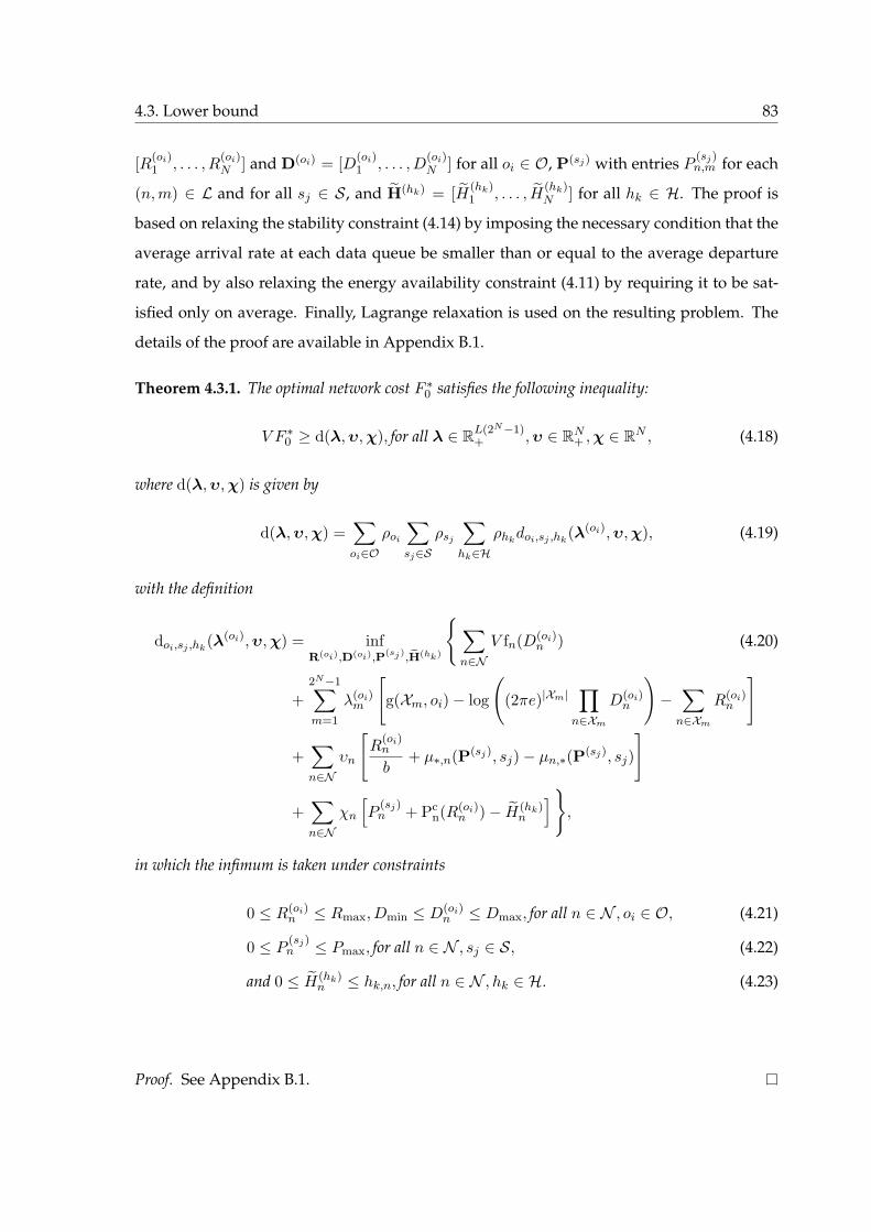
4.3. Lower bound 83
[R(oi)1 , . . . , R
(oi)N ] and D(oi) = [D
(oi)1 , . . . , D
(oi)N ] for all oi ∈ O, P(sj) with entries P (sj)
n,m for each
(n,m) ∈ L and for all sj ∈ S , and H(hk) = [H(hk)1 , . . . , H
(hk)N ] for all hk ∈ H. The proof is
based on relaxing the stability constraint (4.14) by imposing the necessary condition that the
average arrival rate at each data queue be smaller than or equal to the average departure
rate, and by also relaxing the energy availability constraint (4.11) by requiring it to be sat-
isfied only on average. Finally, Lagrange relaxation is used on the resulting problem. The
details of the proof are available in Appendix B.1.
Theorem 4.3.1. The optimal network cost F ∗0 satisfies the following inequality:
V F ∗0 ≥ d(λ,υ,χ), for all λ ∈ R
L(2N−1)+ ,υ ∈ R
N+ ,χ ∈ R
N , (4.18)
where d(λ,υ,χ) is given by
d(λ,υ,χ) =∑
oi∈O
ρoi∑
sj∈S
ρsj∑
hk∈H
ρhkdoi,sj ,hk(λ(oi),υ,χ), (4.19)
with the definition
doi,sj ,hk(λ(oi),υ,χ) = inf
R(oi),D(oi),P(sj),H(hk)
∑
n∈N
V fn(D(oi)n ) (4.20)
+2N−1∑
m=1
λ(oi)m
[g(Xm, oi)− log
((2πe)|Xm|
∏
n∈Xm
D(oi)n
)−∑
n∈Xm
R(oi)n
]
+∑
n∈N
υn
[R
(oi)n
b+ µ∗,n(P
(sj), sj)− µn,∗(P(sj), sj)
]
+∑
n∈N
χn
[P
(sj)n + Pc
n(R(oi)n )− H(hk)
n
],
in which the infimum is taken under constraints
0 ≤ R(oi)n ≤ Rmax, Dmin ≤ D
(oi)n ≤ Dmax, for all n ∈ N , oi ∈ O, (4.21)
0 ≤ P(sj)n ≤ Pmax, for all n ∈ N , sj ∈ S, (4.22)
and 0 ≤ H(hk)n ≤ hk,n, for all n ∈ N , hk ∈ H. (4.23)
Proof. See Appendix B.1.
84 Chapter 4. Distributed Data Gathering in Wireless Sensor Networks
4.4 Proposed Policy
In this section, we propose an algorithm designed following the Lyapunov optimization
framework, as developed in [87] [88], to solve the optimization problem (4.16). In particu-
lar, we aim at finding a policy π for problem (4.16) with close-to-optimal performance, by
using Lyapunov optimization with weight perturbation. The technique of weight perturba-
tion, as proposed in [79], is used to ensure that the energy queues are kept close to a target
value. This is done to avoid battery underflow in a way that is reminiscent of the battery
management strategies put forth in [91], and is further discussed below.
The proposed policy operates by approximately minimizing at each slot the one-slot con-
ditional Lyapunov drift plus penalty [88] of the energy and data queues ((4.12) and (4.13),
respectively) of the network. The optimization is done in an on-line fashion based on the
knowledge of the current channel state S(t), observation state O(t), data queue sizes U(t)
and energy queue sizes E(t). Note that no knowledge of the statistics of the states is re-
quired, as it is standard with Lyapunov optimization techniques [87, 88].
Algorithm: Fix a weight θ = [θ1, . . . , θN ] ∈ RN+ and a parameter V > 0. At each time-slot
t, based on the values of the queues E(t) and U(t), channel states S(t) and observation states
O(t), perform the following:
• Energy Harvesting: For each node n ∈ N , choose Hn(t) that minimizes (En(t)−θn)Hn(t)
under the constraint 0 ≤ Hn(t) ≤ Hn(t). That is, if (En(t) − θn) < 0, perform energy
harvesting and store the harvested energy, i.e., set Hn(t) = minθn − En(t), Hn(t);
otherwise, perform no harvesting, i.e., set Hn(t) = 0;
• Rate-Distortion Optimization: Choose the source acquisition/compression rate vector
R(t) = r = [r1, . . . , rN ] and the distortion levels D(t) = d = [d1, . . . , dN ] to be an
optimal solution of the following optimization problem:
minimizer,d
∑
n∈N
[Un(t)rn − (En(t)− θn)Pcn(rn) + V fn(dn)] , (4.24)
subject to the rate-distortion region constraint (4.8), and to the constraints 0 ≤ rn ≤
Rmax and Dmin ≤ dn ≤ Dmax for all n ∈ N ;
• Power Allocation: Define the weight of a link (n,m) ∈ L as
Wn,m(t) = maxUn(t)− Um(t)− δ, 0, (4.25)

4.4. Proposed Policy 85
where δ = lmaxµmax +Rmax, and choose the transmission power matrix P(t) = p with
entries pn,m for (n,m) ∈ L to be an optimal solution of the following optimization
problem:
maximizep
∑
n∈N
∑
m∈N\n
Cn,m(p,S(t))Wn,m(t) + (En(t)− θn)pn
, (4.26)
where pn =∑
m∈N\n pn,m, subject to constraints 0 ≤ pn ≤ Pmax, for each (n,m) ∈ L;
• Queues Update: Update E(t) and U(t) according to (4.12) and (4.13), respectively.
Remark 4.4.1. In the algorithm proposed above, the energy availability constraint (4.11) is not
explicitly imposed. However, as discussed in Section 4.5, with a proper choice of the weight vector θ,
the battery levels are guaranteed to be such that condition (4.11) is never violated. In other words, the
effect of the weight vector θ is to ensure that, whenever the algorithm requires to draw energy from the
batteries for transmission or acquisition/compression, there is energy available at the corresponding
nodes to satisfy the request.
4.4.1 Price-based Distributed Optimization
While the Energy Harvesting step can be performed independently by all nodes, the Rate-
Distortion Optimization problem (4.24) and the Power Allocation problem (4.26) require cen-
tralized optimization. Decentralized implementations of the Power Allocation problem (4.26)
are discussed in many works, see, e.g., []. Here we discuss how to (approximately) solve
the Rate-Distortion Optimization problem (4.24) in a distributed fashion via dual decomposi-
tion [92] [93]. To this end, we introduce the Lagrange multipliers λ ∈ R2N−1+ for the 2N − 1
coupling constraints (4.8), thus obtaining the Lagrangian function for problem (4.24):
L(r,d,λ) =∑
n∈N
[Un(t)rn − (En(t)− θn)Pcn(rn) + V fn(dn)] (4.27)
+∑
m
λm
g(Xm,O(t))− log
(2πe)|Xm|
∏
l∈Xm
dl
−
∑
l∈Xm
rl
,
where the second sum runs over all the 2N − 1 subsets Xm of N . We will use the notation
Xm for the subsets of N throughout the rest of the paper. Moreover, the dual function for
problem (4.24) is
G(λ) = infr,dL(r,d,λ), (4.28)

86 Chapter 4. Distributed Data Gathering in Wireless Sensor Networks
with constraints 0 ≤ rn ≤ Rmax and Dmin ≤ dn ≤ Dmax and the Lagrange dual problem is
given by
maximizeλ0
G(λ). (4.29)
Following the dual decomposition approach [92] [93], the problem of calculating the dual
function (4.28) for a given multiplier vector λ can be decomposed into N local optimization
subproblems, one for each node n ∈ N . Moreover, solution of the dual problem (4.29) can
be performed in an iterative fashion using the subgradient method [92], as it is standard
practice [92] [93]. This leads to the following price-based distributed iterative solution of
the dual problem (4.29) for time slot t:
Initialize λ(1) 0. Then, for each iteration τ = 1, 2, . . .:
• For the given λ(τ) = λ, each source node n solves the local optimization problem
minimize0≤rn≤Rmax, Dmin≤dn≤Dmax
Un(t)rn−(En(t)−θn)Pcn(rn)+V fn(dn)−(log(dn)+rn)
∑
m: n∈Xm
λm,
(4.30)
obtaining the optimal values (r∗n(λ), d∗n(λ));
• The dual variables λ are updated using the subgradient method [92, Sec. 6.1] as
λ(τ + 1) = λ(τ) + ǫτa(λ(τ)), (4.31)
where ǫτ is a positive scalar step size and
a(λ) =∑
m
g(Xm,O(t))− log(2πe)|Xm| −∑
n∈N
log(d∗n(λ)) + r∗n(λ) (4.32)
is a subgradient of function G(λ).
With various choices for the weights ǫτ (e.g., ǫτ = 1/τ ), due to the concavity of function
G(λ), the procedure above is guaranteed to converge to the optimal value of the dual prob-
lem (4.29) [92, Sec. 3.4]. Moreover, under the given assumptions, problem (4.24) is convex
and satisfies Slater’s condition [94]. Therefore, strong duality holds, which guarantees that
the optimal value of the dual problem (4.29) coincides with the optimal value of (4.24), and
the optimal value of (4.29) is attained at some value λ∗. However, in order for the illustrated
iterative procedure to converge to an optimal solution (r∗,d∗) of problem (4.24), we need

4.5. Performance Analysis 87
that the value of the pair (r,d) at which the infimum in (4.28) is attained for λ = λ∗4 co-
incide with the optimal pair for the original problem (4.24). This can be guaranteed if the
Lagrangian function L(r,d,λ) is strictly convex in (r,d) [92, Sec. 3.4]. As proposed in [95]
this can be enforced by adding a small term ǫ(||r||2 + ||d||2) to L(r,d,λ) while performing
the minimization (4.28), foe some ǫ > 0. Although this operation is bound to make the so-
lution only approximate, the quality of the approximation can be controlled by keeping ǫ
small.
4.5 Performance Analysis
In this section, we provide analytical insights into the performance of the proposed
policy. To this end, we define the parameters βn = min αn, 1 (recall (4.10)) and γn =
supDmin≤dn≤Dmax
[fn(dn)−fn(Dmax)log(dn/Dmax)
], which is finite under the given assumptions.
Theorem 4.5.1. Under the proposed algorithm with vector θ = [θ1, . . . , θN ] given by θn = γnβnV +
αnRmax + Pmax, we have that:
1. The data queue and the energy queue of all nodes are bounded as:
0 ≤ En(t) ≤ θn, (4.33)
and 0 ≤ Un(t) ≤ γnV +Rmax, (4.34)
respectively, for all nodes n ∈ N and all times t;
2. When a node n ∈ N allocates a non-zero power to any of its outgoing links (i.e., Pn(t) > 0),
and/or when it chooses a non-zero source acquisition rate (i.e., Rn(t) > 0), thus expending
energy for source acquisition/compression, we have that:
En(t) ≥ αnRmax + Pmax. (4.35)
This condition guarantees that the energy availability constraint (4.11) is satisfied for all nodes
n ∈ N and all times t (see Remark 4.4.1 and Remark 4.5.2).
3. The overall cost F π0 (4.16) achieved by the proposed scheme satisfies the bound
F π0 =∑
n∈N
F πn ≤ F∗0 +
B
V, (4.36)
4This pair exists by Weierstrass theorem [92].

88 Chapter 4. Distributed Data Gathering in Wireless Sensor Networks
where F ∗0 is the optimal cost of problem (4.16) and the finite constant B is defined as B =
N(µmax(µmax +Rmax) +R2
max/2)+ N/2(H2
max + α2nR
2max + P 2
max + 2αnRmaxPmax) +
N(δlmaxµmax +H2max/4).
Proof. See Appendix B.3.
Remark 4.5.2. The fact that (4.35) implies that the proposed algorithm satisfies the energy availabil-
ity constraint (4.11) at each time-slot follows since each node n ∈ N cannot consume an energy larger
that αnRmax + Pmax in a time-slot. In fact, αnRmax is the maximum energy spent for compressing
the acquired data and Pmax is the maximum transmission energy consumption.
Remark 4.5.3. Following [96], under the modified stability requirement
lim supT→∞
1
T
T−1∑
t=1
Un(t) <∞, for all n ∈ N , (4.37)
the proposed algorithm can be proved to guarantee near-optimal performance with probability one.
4.6 Extension with side information at the sink
We now consider an extended version of the problem studied thus far, in which the sink
node d, rather than being the final destination for the sources measured at the sensors, acts
as a cluster head and communicates to a network collector node c (see Fig. 4.1), on a commu-
nication link modeled as for any other pair of node (see Sec. 4.2.1). The key novel aspect of
this extended model is that node d can measure a source correlated with that of the sensors
and use such side information to improve the system performance. Specifically, thanks to
the side information available at node d, the rate requirements for communication from the
sensors to d can be reduced. However, node d, which is powered by energy-harvesting as
all the sensors, also needs to communicate with node c. Therefore, a new trade-off arises
between the energy allocated by d to acquire side information and that used by d to com-
municate with c.
We now discuss how the model discussed in Sec. 4.2 needs to be modified in order to
account for the different setting of interest here. First, the destination d acquires a source
which is correlated with the sensor’s measures with a rate Rd(t). This affects the rate-
distortion constraints (4.8) in that the entropy function g(X ,O(t)) should now be condi-

4.6. Extension with side information at the sink 89
tioned on the side information available at the receiver (see, e.g., [97]). This leads to mod-
ified rate-distortion constraints (4.8) with a function g(X ,O(t), Rd(t)) that depends also on
Rd(t). An example of this function will be given in Sec. 4.7. The energy used for acquiring
the side information is given by Pcd(Rd(t)) = αdRd(t) similar to all other nodes. Moreover,
the data queue at node d evolves as
Ud(t+ 1) ≤ max Ud(t)− µd,c(t), 0+ µ∗,d(t), (4.38)
where µd,c(t) and µ∗,d(t) represent, respectively, the transmitted and received data at time t,
and transmission is to the collector node c. Note that no other node is connected to the net-
work collector c apart from d. The energy queue Ed(t), instead, evolves according to (4.12).
Finally, P(t) and S(t) are extended to consider the additional link (d, c) ∈ L and the rate
achievable on that link is given by Cd,c(P(t),S(t)), which is assumed to have the same prop-
erties as for all other links (see Sec. 4.2). We refer to the power used for transmission by node
d as Pd.
In what follow we modify the algorithm proposed in Section 4.4 in order to address the
new setting outlined above. The modified algorithm works as follows:
• Energy Harvesting: Follow the same procedure as for the algorithm discussed in Sec. 4.4,
for all nodes including node d;
• Rate-Distortion Allocation: Choose Rn(t) and Dn(t), n = 1, . . . , N , and Rd(t) to be the
optimal solution of the following optimization problem:
minimize(r,d),rd
∑
n∈N
[Un(t)rn − (En(t)− θn)Pcn(rn) + V fn(dn)] + (4.39)
(Ed(t)− θd)Pcd(rd), (4.40)
subject to:
∑
n∈X
rn ≥ g(X ,O(t), rd)− log
((2πe)|X |
∏
n∈X
dn
), ∀X ⊆ N , (4.41)
and to constraints 0 ≤ rn ≤ Rmax and Dmin ≤ dn ≤ Dmax for all n ∈ N and 0 ≤ rd ≤
Rmax;
• Power Allocation: Define the weight of a link (n,m) ∈ L 5 as (4.25) and choose the
transmission power matrix P(t) = p with entries pn,m for (n,m) ∈ L to be an optimal5We remind that L is extended to consider the link (d, c).

90 Chapter 4. Distributed Data Gathering in Wireless Sensor Networks
solution of the following optimization problem:
maximizep
∑
n∈N
∑
m∈N\n
Cn,m(p,S(t))Wn,m(t) + (En(t)− θn)pn
+ (4.42)
Cd,c(p,S(t))Wd,c(t) + (Ed(t)− θd)pd, (4.43)
subject to constraints 0 ≤ pn ≤ Pmax, for each (n,m) ∈ L.
• Queues Update: Update E(t) and Ed(t) according to (4.12), U(t) according to (4.13) and
Ud(t) according to (4.38).
The algorithm proposed above is a simple modification of the algorithm proposed in
Sec. 4.4 that accounts for the need to allocate rate and power also for node d. It can be
proved that the algorithm has similar optimality properties as the algorithm of Sec. 4.4, as
summarized in Theorem 4.5.1. We omit a formal statement of this result here, since it is a
straightforward extension of Theorem 4.5.1.
4.7 Numerical results
In this section we provide an example application of the model studied in this paper and
of the results reported above, via some numerical results. We consider the network topology
of Fig. 4.1, where the set N of nodes of the network gather correlated data to the sink node
d. We first consider the set-up without side information studied in Sec. 4.2- 4.5. We assume
that nodes 1, 2, 3 collects the measurements, while nodes 4, 5 are only used as relays (or
equivalently measure constant sources). The sources measured at nodes 1, 2, 3 are jointly
Gaussian with zero mean and correlation matrix
O(t) =
1 ρ ρ
ρ 1 ρ
ρ ρ 1
, (4.44)
with correlation coefficient ρ ∈ [0, 1]. The channel state matrix S(t) has independent entries,
is i.i.d. across time-slots and Rayleigh distributed, while the harvestable energy H(t) has
independent entries, is i.i.d. across time-slots and uniformly distributed within [0, Hmax].
Moreover, we consider the capacity function Cn,m(P(t),S(t)) = log(1 + Pn,m(t)Sn,m(t))
for all (n,m) ∈ L, the entropy function given for the rate-distortion constraints (4.8) given

4.7. Numerical results 91
0
500
1000
1500
2000
2500
3000
3500
4000
4500
5000
0 1000 2000 3000 4000 5000 6000 7000
Qu
eue
size
V
MaxAverage
0
500
1000
1500
2000
2500
3000
3500
4000
4500
5000
0 1000 2000 3000 4000 5000 6000 7000
Qu
eue
size
V
MaxAverage
Figure 4.3. Maximum and average network queue size vs V for fixed source correlation ρ. (ρ = 0.5)
by (4.9), and cost function fn(Dn(t)) = Dn(t) for all n ∈ N . Moreover, we set the numerical
values αn = 1, Hmax = 3, Dmin = 0.001 and Pmax = αnRmax, withRmax = g(1, 2, 3,O(t))−
log((2πeDmin)
3).
We first examine the effect of parameter V , which was shown in Theorem 4.5.1 to rule the
(V, 1/V ) trade-off between the size of the queues and the additive gap to the lower bound
of Theorem 4.3.1. To this end, in Fig. 4.3 and 4.4, we fix ρ = 0.5 and we plot the maximum
and average network queue size (Fig. 4.3), and average sum-distortion F π0 (Fig. 4.4) as a
function of the parameter V . Confirming the results of Theorem 4.5.1, we observe a linear
increase with respect to V of the maximum and time average network queue size, while the
sum-distortion F π0 gradually converges to the lower bound F ∗0 . We remark that most of the
decrease (93% in the sum-distortion) takes place by varying V from V = 225 to V = 1000.
Our numerical results also show that the average energy consumption for V large enough
is constant and is given for 83% by the power required for transmission and the remaining
for compression.
We now evaluate the impact of the source correlation parameter ρ on the network perfor-
mance. As explained, a larger correlation enables more flexibility in the energy consumption
across the nodes, and thus we expect enhanced performance in terms of both queue sizes

92 Chapter 4. Distributed Data Gathering in Wireless Sensor Networks
0.5
0.52
0.54
0.56
0.58
0.6
0.62
0.64
0.66
0 1000 2000 3000 4000 5000 6000 7000
F0
π
V
0.5
0.52
0.54
0.56
0.58
0.6
0.62
0.64
0.66
0 1000 2000 3000 4000 5000 6000 7000
F0
π
V
Figure 4.4. Fπ0
vs V for fixed source correlation ρ. (ρ = 0.5)
200
300
400
500
600
700
800
900
0 0.1 0.2 0.3 0.4 0.5 0.6 0.7 0.8 0.9 1
Qu
eue
size
ρ
MaxAverage
Figure 4.5. Maximum and average network queue size vs source correlation ρ. (V = 1000)
and sum-distortion. To elaborate, Fig. 4.5 and Fig. 4.6 plot the average and maximum net-
work queue size and the sum-distortion F π0 , respectively, versus the correlation ρ ∈ [0, 1).

4.7. Numerical results 93
0.15
0.2
0.25
0.3
0.35
0.4
0.45
0.5
0.55
0.6
0 0.1 0.2 0.3 0.4 0.5 0.6 0.7 0.8 0.9 1
F0
π
ρ
Figure 4.6. Fπ0
vs source correlation ρ. (V = 1000)
As expected, the effect of the correlation ρ is to reduce both the network queue size and the
sum-distortion F π0 . We emphasize that this is due to the fact that increasing ρ corresponds
to increasing the correlation between the sources, which returns a lower entropy g(X ,O(t)).
Since the optimization is driven by the rate-distortion constraints (4.8), reducing the value of
g(X ,O(t)) reduces the exogenous rate Rn(t) needed at each source to achieve a certain dis-
tortion level Dn(t). As a consequence, increasing ρ reduces the time average and maximum
network queue size and, at the same time, reduces the value F π0 .
Finally, we evaluate the performance gain of the scenario of Section 4.6, in which the sink
node d acts as a cluster head and can measure a source correlated with that of there other
sensors to improve the system performance and communicate to node c (see Fig. 4.1). To
this end, we substitute the entropy function g(X ,O(t)) with g(X ,O(t), Rd(t)), to take into
account the side information added by d. Given the correlation matrix (4.44) for which we
determined the results of this Section, we can derive that, if we consider that node d can
make a measurement that is rate limited to Rd(t), the matrix O(t) becomes
O(t) =
1− ρρd ρ(1− ρd) ρ(1− ρd)
ρ(1− ρd) 1− ρρd ρ(1− ρd)
ρ(1− ρd) ρ(1− ρd) 1− ρρd
, (4.45)

94 Chapter 4. Distributed Data Gathering in Wireless Sensor Networks
0
0.1
0.2
0.3
0.4
0.5
0.6
0.7
0.8
0 0.1 0.2 0.3 0.4 0.5 0.6 0.7 0.8 0.9 1
F0
π
ρ
V = 1
Figure 4.7. Fπ0
vs source correlation ρ for the model with side information. Dashed line: optimized Rd(t);
Solid line: Rd(t) = 0.
where ρd = 1 − 2−Rd(t). We consider the same simulation parameters as before and we
additionally set αd = 1. Fig. 4.7 plots the sum-distortion F π0 , versus the correlation ρ ∈ [0, 1).
As expected, the effect of the side information of node d is to reduce both the network queue
size and the sum-distortion F π0 , even for V = 1 and for all ρ > 0. As expected, this is
due to the fact that adding side information Rd(t) corresponds to increasing the correlation
between the sources, which returns a lower entropy g(X ,O(t), Rd(t)) with respect to the
previous case. Moreover, we observed that increasing V produces results similar to the ones
observed in Fig. 4.3 and Fig. 4.4, confirming that the results of Theorem 4.3.1 can be extended
also to the policy of Section 4.6.
4.8 Conclusions
Energy harvesting poses new challenges in terms of energy management of wireless
networks. In sensor networks, these challenges are compounded by the need to balance the
energy consumed for source coding tasks (i.e., compression) with that used for transmission.
Moreover, the correlation among the sources measured by different sensors, if leveraged

4.8. Conclusions 95
via distributed source coding, open up the possibility to exploit spatial energy trade-offs
across the sensors. Based on the above, this work has proposed a dynamic optimization
strategy that jointly optimizes source coding and transmission for time-varying sources and
channels. The proposed technique, based on Lyapunov optimization, has been shown to be
characterized by a (V, 1/V ) trade-off in terms of the additive optimality gap and the queue
and battery sizes. Numerical results have demonstrated the critical role of source correlation
and distributed source coding in the system performance.


Chapter 5Conclusions
In this Thesis we discussed different cooperation principles to be used for improving the
performance of wireless ad hoc networks and we proposed efficient stochastic optimization
techniques, both from a centralized and a distributed perspective.
In the first part of the work, we found optimal cooperator selection policies for multihop
networks with MIMO transmission and a single flow. We modeled the cooperator selection
process through a suitable Markov chain, that we reduced according to a novel pruning tech-
nique that cuts states with negligible impact on the optimal solution. The pruning technique
has been integrated into an advanced solver based on real time dynamic programming and
we showed the effectiveness of this approach in terms of optimality gap and computational
complexity. Our solver is able to find policies within an additional tunable cost with respect
to the optimal and allows to derive the Pareto efficient frontier in terms of transmission
cost vs delay for arbitrary networks. Using selected application examples we discussed the
impact of
1) the set of nodes that cooperate at each transmission opportunity,
2) the selection of the optimization criteria, i.e., energy vs delay minimization,
3) the maximum number of nodes that are allowed to cooperate.
Starting from the results of the optimal policies, we then proposed three algorithms for the
selection of cooperating nodes in multihop wireless networks in a distributed fashion. The
aim of these policies is the minimization of a cost obtained as a linear combination of delay

98 Chapter 5. Conclusions
and energy consumption, as for the optimal policies. The three policies allow the selection
of the cooperating nodes at a local level among the nodes that receive the message at each
hop, thus being viable for a practical implementation. They differ for various look-ahead
strategies that realize a locally greedy approach for the solution of the otherwise complex
global optimization problem. In a performance comparison with the optimal centralized
approach, the heuristics exhibit very limited losses and in any case outperform approaches
that had been presented in the literature, thus being of interest for their use in future net-
works. We then extended the system model to accommodate for multiple concurrent flows
and we solved the joint routing and transmission scheduling problem in wireless ad hoc net-
works in the presence of multi-user interference. The problem has been formulated using
linear programming and, for the sake of an efficient implementation, subsequently solved
through a shortest path optimization method exploiting the A∗ heuristic search [58]. Nu-
merical results show that cooperative transmissions can respectively provide benefits of up
to 25% and 58% for the energy and delay with respect to a non-cooperative approach.
In the second part of the Thesis, we designed routing protocols in cognitive radio multi-
hop networks, where primary and secondary nodes coexist over the same spectral resource.
We first proposed a spectrum leasing solution to this problem, wherein secondary nodes
are granted the possibility to transmit by the primary network in exchange for forwarding
primary packets. We considered as the primary network goal the maximization of an ap-
propriate trade-off between throughput and energy gains. The optimization objective was
attained through the cooperation of secondary networks, whereas secondary nodes enforce
minimum QoS requirements when deciding whether or not to cooperate. We formulated the
problem as a Markov Decision Process and we showed that, in particular, the problem is an
instance of stochastic routing. We then proposed two heuristic policies with lower complex-
ity and our numerical results lend evidence to the throughput and energy gains that can be
attained by the proposed spectrum leasing approach by the primary network, all the while
allowing also the secondary nodes to transmit. Moreover, the heuristic policies are shown
to provide flexible solutions that perform close to the optimal policy.
In the last part of the work, we looked into an energy harvesting scenario, which poses
new challenges in terms of energy management of wireless networks. In sensor networks,
these challenges are compounded by the need of balancing the energy consumed for source

5.1. Future directions 99
coding tasks (i.e., acquisition and compression) with that used for transmission. Moreover,
the correlation among the sources measured by different sensors, if leveraged via distributed
source coding, open up the possibility to exploit spatial energy trade-offs across the sensors.
Based on the above, in this work we proposed a dynamic optimization strategy that jointly
optimizes source coding and transmission for time-varying sources and channels. The pro-
posed technique, based on Lyapunov optimization, has been shown to be characterized by
a (V, 1/V ) trade-off in terms of the additive optimality gap and the queue and battery sizes.
Numerical results have demonstrated the critical role of source correlation and distributed
source coding in the system performance.
All the forms of cooperations analyzed in this Thesis showed beneficial advantages in
terms of the different network performance metrics considered. This confirms that cooper-
ation between nodes in a wireless ad hoc network is effective and can be considered as a
viable solution in practical scenarios.
5.1 Future directions
All the results obtained here are useful performance bounds for the design of practical
cooperation schemes. In fact, it is important when designing a routing protocol to have, as
a metric of comparison, the optimal performance that can be achieved if the information
available about the network and the computational complexity are not an issue.
Moreover, from the first part of this Thesis we derived an analytical tool that works with
any scenario where outage probabilities can be obtained analytically and is thus applicable
as well to different network optimization problems.
As a final reminder, note that all the results of this Thesis are based on the assumption
that all the nodes are trustful and they do not act selfishly.


Appendix A
A.1 Outage probability computation, Single Antenna Nodes (NA =
NR = 1)
When NA = NR = 1, the capacity turns out to be the logarithm of a linear combination
of central chi square random variables, i.e., C = log2 (1 + ρy), where y is the sum of NT
exponential random variables with means Σk, k = 1, 2, . . . , NT. For the general case where
some of the means Σm are equal, i.e. Σk = Σm for some k and m, the outage probability
can be obtained using the result in [98]. By letting σk, rk and Nσ be the unique means,
their multiplicity and the number of equality classes, respectively, with k = 1, 2, . . . , Nσ and∑Nσ
k=1 rk = NT, the outage probability for node n when nodes in set a transmit is found as
pout(a, n) = 1−
( Nσ∏
j=1
σ−rjj
) Nσ∑
k=1
rk∑
ℓ=1
φk,ℓ(−σ−1k )
σ−rk+ℓ−1k
f1
(σ−1k
2R − 1
ρ, rk − ℓ
), (A.1)
where f1(a, b) is the cumulative distribution function of a Poisson variable of parameter a,
φk,ℓ(x) = (−1)ℓ−1∑
Ω(Nσ ,k,ℓ)
∏
j
(ij + rj − 1
ij
)τj(x) , (A.2)
the set Ω(Nσ, k, ℓ) defines partitions of ℓ − 1 through the positive integer indices ij , such
that∑Nσ
j=1,6=k ij = ℓ− 1 and τj(x) = (σ−1j + x)−(rj+ij). Simpler expressions for the outage
probability hold when all the means are equal or when all the means are different, i.e., rk = 1,
k = 1, 2, . . . , NT, see [99, Section 3.3.1, p. 47] and [100].
101
102 Appendix A.
A.2 Proof of Lemmas and Theorems
A.2.1 Proof of Lemma 2.3.1
Proof. Let f(x, a, y)def= c(x, a, y) + γJ(y). For mapping T (·) (P) we can write:
(TJ)(x) = mina∈A(x)
[∑
y∈N (x)
pxy(a)f(x, a, y)
]
(1)
≤ mina∈A′(x)
[∑
y∈N (x)
pxy(a)f(x, a, y)
]
= mina∈A′(x)
[∑
y∈N ′(x)
pxy(a)f(x, a, y) +∑
y∈N (x)\N ′(x)
pxy(a)f(x, a, y)
]
(2)
≤ mina∈A′(x)
[∑
y∈N ′(x)
p′xy(a)f(x, a, y) +∑
y∈N (x)\N ′(x)
pxy(a)f(x, a, y)
]
(3)
≤ mina∈A′(x)
[∑
y∈N ′(x)
p′xy(a)f(x, a, y) +(cmax + γJ(x)
) ∑
y∈N (x)\N ′(x)
pxy(a)
]
(4)
≤ mina∈A′(x)
[∑
y∈N ′(x)
p′xy(a)f(x, a, y) +M(x)
(cmax + γmax
x∈SJ(x)
)]
= (TpJ)(x) + ∆(x) , (A.3)
where (1) follows as the minimum taken over a subset A′(x) ⊆ A(x) cannot be smaller than
the minimum taken over the original set A(x). (2) follows from (2.8) as∑
y∈N ′(x) pxy(a) ≤ 1.
(3) follows from the definition of upper bound J(x) and noting that c(x, a, y) ≤ cmax for all
states x, y and actions a. (4) follows from the definition of M(x).
A.2.2 Proof of Lemma 2.3.2
Proof. Let f(x, a, y)def= c(x, a, y) + γJ(y). By definition of mapping T (·) we can write:
(TJ)(x) = mina∈A(x)
g(x, a)
(1)= min
a∈A′(x)
[∑
y∈N ′(x)
pxy(a)f(x, a, y) +∑
y∈N (x)\N ′(x)
pxy(a)f(x, a, y)
]
(2)
≥ mina∈A′(x)
[∑
y∈N ′(x)
p′xy(a)
(∑
y∈N ′(x)
pxy(a)
)f(x, a, y)
]
(3)
≥ (1− η)(TpJ)(x) , ∀x ∈ S . (A.4)

A.2. Proof of Lemmas and Theorems 103
(1) follows from the assumption made in the lemma, (2) follows as the second sum is greater
than or equal to zero, and by the definition of p′xy(a) (Eq. (2.8)). For (3) consider the follow-
ing
1 =∑
y∈N ′(x)
pxy(a) +∑
y∈N (x)\N ′(x)
pxy(a) ≤∑
y∈N ′(x)
pxy(a) +M(x) ≤∑
y∈N ′(x)
pxy(a) + η . (A.5)
Hence, we can further write∑
y∈N ′(x) pxy(a) ≥ 1− η, which proves the lemma.
A.2.3 Proof of Theorem 2.3.4
Proof. From Lemma 2.3.1 we have:
(TJ)(x) ≤ (TpJ)(x) +M(x)[cmax + γmaxx∈S
J(x)](1)
≤ (TpJ)(x) + ∆ , ∀x ∈ S , (A.6)
where inequality (1) follows from the assumption made for M(x). Hence:
(TJ)(x) ≤ (TpJ)(x) + ∆ , ∀x ∈ S . (A.7)
Now, applying mapping Tp(·) to both sides gives:
(Tp(TJ))(x) ≤ (T 2p J)(x) + γ∆ , ∀x ∈ S , (A.8)
where the expression on the RHS follows from Lemma 1.1.2 of [28]. Re-applying (A.7) (LHS):
(T 2J)(x)−∆ = (T (TJ))(x)−∆ ≤ (T 2p J)(x) + γ∆ , ∀x ∈ S , (A.9)
and hence (T 2J)(x) ≤ (T 2p J)(x) + γ∆+∆. Repeated iterations of this procedure leads to:
(T kJ)(x) ≤ (T kp J)(x) +k−1∑
j=0
γj∆ , ∀x ∈ S . (A.10)
Now, taking the limit as k → +∞ to both sides of (A.10) leads to:
J∗(x) ≤ J∗p (x) +
∆
1− γ, ∀x ∈ S , (A.11)
which proves (i). For (ii), from Lemma 2.3.2 we have, (TJ)(x) ≥ δ(TpJ)(x), where δ =
1− ∆cmax+γmaxx∈S J(x)
. Applying Tp(·) to both sides of this last inequality gives
(Tp(TJ))(x) ≥ (Tpδ(TpJ))(x)def= (Tp(TpJ))(x) , (A.12)

104 Appendix A.
where Tp(·) is mapping Tp(·) (Eq. (2.10)) with discount factor γ = γδ. Moreover, application
of Lemma 2.3.2 to the LHS of the above inequality returns
(T 2J)(x)δ−1 ≥ (Tp(TJ))(x) ≥ (Tp(TpJ))(x) . (A.13)
Repeated iterations of this procedure lead to (T kJ)(x) ≥ δ(T k−1p (TpJ))(x). Now, taking the
limit k → +∞ to both sides of the previous inequality gives J∗(x) ≥ δJ∗p (x), where J∗
p (x) is
the optimal cost function for problem P ′ with discount factor γ = γδ.
A.2.4 Proof of Proposition 2.3.6
Proof. SetN (x) \N ′(x) contains the pruned states. These are states y containing nodes with
small probability of receiving the message at the next hop i+ 1, given x. From Lemma 2.3.5
the maximizing action a′max = argmaxa∈A′(x)[∑
y∈N (x)\N ′(x) pxy(a)] corresponds to the case
where the maximum number of nodes allowed by A′(x) transmit, as all receiving nodes
n ∈ T −(x) maximize their reception probability, namely psucc(n, a), for this action. Thus,
a′max = amax, where amax was defined in Lemma 2.3.5. This implies that
M(x) =∑
y∈N (x)\N ′(x)
pxy(amax) (A.14)
which is, by definition, the probability that the system in hop i+1 will move to state y when
action amax is selected. If we define y ∈ N (x)\N ′(x) as any state for which: 1) all nodes that
were successful in x are still successful in y and 2) at least one node in V(x) is successful,
then by the way we constructed V(x) we have that
M(x) =∑
y∈N (x)\N ′(x)
pxy(amax) =∑
Ψ(|V(x)|)
|V(x)|∏
j=1
v(j)ξ(j)(1− v(j))1−ξ(j) (A.15)
and the inequality in (2.16) is granted by the construction algorithm.

Appendix B
B.1 Proof of Theorem 4.3.1
Proof. Define as φ∗ the optimal value of the following problem:
minimize V∑
n∈N
∑
oi∈O
ρoi
K∑
k=1
ϑ(oi)k fn
(D
(oi)n,[k]
)(B.1)
subject to:
g(X , oi)− log(2πe)|X |∏
n∈X
D(oi)n,[k] ≤
∑
n∈X
R(oi)n,[k], for all X ⊆ N , oi ∈ O, k ∈ [1, . . . ,K], (B.2)
∑
oi∈O
ρoi
K∑
k=1
ϑ(oi)k
R(oi)n,[k]
b+∑
si∈S
ρsi
K∑
k=1
(si)k µ∗,n(P
(si)k , si)
≤∑
si∈S
ρsi
K∑
k=1
(si)k µn,∗(P
(si)k , si), for all n ∈ N ,
(B.3)
∑
si∈S
ρsi
K∑
k=1
(si)k
(P
(si)n,[k]
)+∑
oi∈O
ρoi
K∑
k=1
ϑ(oi)k Pc
n
(R
(oi)n,[k]
)
=∑
hi∈H
ρhi
K∑
k=1
ϕ(hi)k H
(hi)n,[k], for all n ∈ N ,
(B.4)
0 ≤ ϑ(oi)k ,
(si)k , ϕ
(hi)k ≤ 1, for all oi ∈ O, si ∈ S, hi ∈ H, k ∈ [1, . . . ,K],
K∑
k=1
ϑ(oi)k = 1,
K∑
k=1
(si)k = 1,
K∑
k=1
ϕ(hi)k = 1, for all oi ∈ O, si ∈ S, hi ∈ H,
0 ≤ R(oi)n,[k] ≤ Rmax, Dmin ≤ D
(oi)n,[k] ≤ Dmax, for all n ∈ N , oi ∈ O, k ∈ [1, . . . ,K], (B.5)
0 ≤ P(si)n,[k] ≤ Pmax, for all n ∈ N , si ∈ S, k ∈ [1, . . . ,K], (B.6)
and 0 ≤ H(hi)n,[k] ≤ hi,n, for all n ∈ N , hi ∈ H, k ∈ [1, . . . ,K], (B.7)
105

106 Appendix B.
where the minimization is done over variables ϑ(oi)k , (si)k , ϕ(hi)k , R(oi)
n,[k], D(oi)n,[k], H
(hi)n,[k] and P (si)
n,[k]
for all n ∈ N , oi ∈ O, si ∈ S , hi ∈ H and k ∈ [1, . . . ,K], with K = 2N + 2. VariablesR
(oi)n,[k]
Kk=1
andD
(oi)n,[k]
Kk=1
can be interpreted, respectively, as the set of rates and distor-
tions selected by node n ∈ N when the source state is O(t) = oi. Specifically, node n selects
rate R(oi)n,[k] and distortion D
(oi)n,[k] with probability ϑ
(oi)k when the source state is O(t) = oi.
VariablesP
(si)n,m,[k]
Kk=1
can be seen as the transmission powers allocated to link (n,m) ∈ L,
when the channel state S(t) = si. Each power P (si)n,m,[k] is selected with probability
(si)k if
S(t) = si. Finally, variablesH
(hi)n,[k]
Kk=1
represent the harvested energy when the energy
harvesting state is H(t) = hi = [hi,1, . . . , hi,N ]. Each energy H(hi)n,[k] is selected with probabil-
ity ϕ(hi)k if H(t) = hi. Note that we added the constant V in the optimization function for
our later analysis.
Theorem B.1.1. The optimal network cost F ∗0 satisfies the following inequality:
V F ∗0 ≥ φ
∗, (B.8)
where φ∗ is the optimal value of the optimization problem (B.1). The proof of Theorem B.1.1 is in
Appendix B.2.
A generally looser lower bound can be evaluated by the weak duality in Lagrange op-
timization theory [94], which is easily seen to lead to Theorem 4.3.1. In fact, in (4.19), the
parameters λ(oi)m for m = [1, . . . , 2N − 1] and oi ∈ O are the L(2N − 1) Lagrange multipli-
ers corresponding to constraints (B.2), parameters υn for n = [1, . . . , N ] are the Lagrange
multipliers corresponding to constraints (B.3) and parameters χn for n = [1, . . . , N ], are the
Lagrange multipliers corresponding to constraints (B.4).
B.2 Proof of Theorem B.1.1
Proof. We follow an argument similar to the one used in [89]. Consider any stable policy π,
i.e., a policy such that the condition (4.14) is satisfied under π. Since E[µ∗,n(t) + Rn(t)/b −
µn,∗(t)] ≤ (N − 1)µmax +Rmax/b, from [88, Theorem 2.8], constraint (4.14) implies the mean
rate stability constraint and thus the condition
lim supT→∞
1
T
T−1∑
t=0
E
[µ∗,n(t) +
Rn(t)
b
]≤ lim inf
T→∞
1
T
T−1∑
t=0
E[µn,∗(t)], (B.9)
B.3. Proof of Theorem 4.5.1 107
for each node n ∈ N . We thus relax problem (B.1) by substituting (4.14) with (B.9). We fur-
ther relax the energy availability constraint (4.11) by only imposing that the constraint (4.14)
be satisfied on average as
lim supT→∞
1
T
T−1∑
t=0
E[Pn(t) + Pcn(Rn(t))] = lim sup
T→∞
1
T
T−1∑
t=0
E[Hn(t)]. (B.10)
For the relaxed problem, we can show as in [89] that the optimal policy is stationary and
depends only on the source and channel state. From this, by Caratheodory’s theorem [101],
we obtain that the problem at hand is equivalent to (B.1).
B.3 Proof of Theorem 4.5.1
Proof. 1) From the energy harvesting part of the algorithm, we have that En(t) ≤ θn, since
harvesting is performed only when En(t) < θn and the maximum amount of harvested
energy in that case is θn − En(t). This proves (4.33).
We now prove (4.34) by induction on t. Inequality (4.34) holds for t = 0, since Un(0) = 0
for all n. Then, assuming that (4.34) is satisfied for all n at time t, we show that it holds
also for time t + 1. To this end, we consider separately the different possible cases in
which a node n receives or not data from other nodes (i.e., endogenous data) and/or
acquires or not its measurement (i.e., exogenous data). First, if node n receives neither
endogenous nor exogenous data, then we have that Un(t + 1) ≤ Un(t) ≤ γnV + Rmax,
which proves the claim. Second, assume that node n ∈ N receives endogenous, but not
exogenous, data. It follows from (4.26) that, for some node m ∈ N , with m 6= n, we must
have
Un(t) ≤ Um(t)− δ ≤ γnV +Rmax − δ. (B.11)
However, since any node can receive at most lmaxµmax bits per channel use of endogenous
data, we have from (B.11) and the definition δ = lmaxµmax+Rmax that Un(t+1) ≤ γnV ≤
γnV +Rmax, which proves the claim.
We now analyze the case in which node n receives exogenous, but not endogenous, data.
This implies that rn > 0 is obtained from the solution of problem (4.24). We define the

108 Appendix B.
corresponding Lagrangian function as
L(r,d,λ,υ) =∑
n∈N
[Un(t)rn − (En(t)− θn)Pcn(rn) + V fn(dn)] (B.12)
+∑
m
λm
g(Xm,O(t))− log
(2πe)|Xm|
∏
l∈Xm
dl
−
∑
l∈Xm
rl
+∑
n∈N
υn(dn −Dmax),
where we have relaxed the constraints (4.8) and constraints dn ≤ Dmax. The Lagrange
dual function is given by
G(λ,υ) = infr,dL(r,d,λ,υ), (B.13)
where the infimum is taken with the constraints 0 ≤ rn ≤ Rmax and dn ≥ 0, and the dual
problem is given by:
maximizeλ0,υ0
G(λ,υ). (B.14)
Lemma B.3.1. Any dual optimal vector λ∗ (i.e., a vector λ maximizing (B.14)) satisfies the
conditions∑
m: n∈Xm
λ∗m ≤ γnV, (B.15)
for all n ∈ N . Moreover, any primal optimal r∗n satisfies the condition
r∗n = arg min0≤rn≤Rmax
Un(t)rn − (En(t)− θn)Pcn(rn)− rn
∑
m: n∈Xm
λ∗m. (B.16)
The proof of Lemma B.3.1 can be found in Appendix B.4.
According to (B.16) we have that r∗n > 0 is an optimal solution of problem (4.24) only
if the value of the right-hand side of (B.16) evaluated at rn = 0 is larger than the value
obtained by evaluating it at r∗n, which can be expressed, using (4.10), as
Un(t)r∗n + (θn − En(t))αnr
∗n − r
∗n
∑
m: n∈Xm
λ∗m ≤ 0. (B.17)
From (4.33), (B.15) and (B.17), we further obtain:
Un(t) ≤∑
m: n∈Xm
λ∗m ≤ γnV, (B.18)

B.3. Proof of Theorem 4.5.1 109
which implies that a node n receives exogenous data from outside the network only
when Un(t) ≤ γnV . Hence, recalling that Rn(t) ≤ Rmax, we obtain the desired result
Un(t+ 1) ≤ γnV +Rmax.
Finally, if a node n receives both endogenous and exogenous data, we have from (B.11)
that Un(t) ≤ γnV − lmaxµmax. But, since a node n can receive at most lmaxµmax bits per
channel use of endogenous data and Rmax bits per channel use of exogenous data, we
have the desired inequality Un(t + 1) ≤ γnV + Rmax, which completes the proof of part
1).
2) To prove the claim, we need to show that if
En(t) < αnRmax + Pmax, (B.19)
then the following two conditions must be satisfied:
a) the Rate-Distortion problem (4.24) is minimized by choosing Rn(t) = r∗n = 0 (which
implies Pcn(t) = 0) for all n ∈ N ;
b) the Power Allocation problem (4.26) selects a power matrix P(t) such that Pn(t) = 0
for all n ∈ N .
From Lemma B.3.1, and in particular from (B.16), condition a) is verified if
Un(t)rn − (En − θn)Pcn(rn)− rn
∑
m: n∈Xm
λ∗m > 0, for all rn > 0, (B.20)
where we recall that λ∗ is any optimal dual vector of problem (B.14). This is proved by
the following inequalities:
Un(t)rn − (En − θn)αnrn − rn∑
m: n∈Xm
λ∗m > Un(t)rn +γnβnV αnrn − rn
∑
m: n∈Xm
λ∗m
≥ Un(t)rn +γnβnV αnrn − rnγnV
= Un(t)rn + γnV(αn − βn)rn
βn(B.21)
≥ 0,
where the first inequality follows from (B.19) and the assumption of Theorem 4.5.1 that
θn = γnβnV + αnRmax + Pmax; the second from (B.15); and the last inequality follows from
110 Appendix B.
the fact that Un(t) ≥ 0, rn > 0 and from the definition of βn. This proves (B.20) and thus
that condition a) is satisfied if (B.19) holds.
To prove b) we first note that the bound (4.34) implies that the weight (4.25) satisfies the
inequality
Wn,m(t) = maxUn(t)− Um(t)− δ, 0 ≤ γnV − lmaxµmax , (B.22)
for all (n,m) ∈ L and for all time t. We now show by contradiction that condition b)
holds when (B.19) is satisfied. To this end, assume that the power allocation vector P∗
that maximizes (4.26) at time t is such that some entry P ∗n,m is positive. Starting from
P∗, we now obtain a new power allocation vector P, in which we set Pn,m = 0. Clearly,
the power matrix P is also feasible. We demonstrate that the objective function of (4.26)
when evaluated at P∗ is smaller than at P, thus leading to a contradiction. Denoting as
G(P) the objective function of (4.26), this is shown by the following inequalities:
G(P∗)−G(P) =∑
n∈N
∑
l∈N\n
[Cn,l(P∗,S(t))− Cn,l(P,S(t))]Wn,l(t) + (En(t)− θn)P
∗n,m
≤ Cn,m(P∗,S(t))Wn,m(t) + (En(t)− θn)P
∗n,m
≤ Cn,m(P∗,S(t))(γnV − lmaxµmax) + (En(t)− θn)P
∗n,m
≤ (γnV − lmaxµmax)ξP∗n,m + (En(t)− θn)P
∗n,m
< (γnV − lmaxµmax)ξP∗n,m −
γnβnV P ∗
n,m
< 0,
where the first inequality derives from the fact that µn,l(P∗,S(t)) − µn,l(P,S(t)) ≤ 0 for
all l 6= m (Property 2), the second from (B.22), the third from Property 1 and the fourth
from (B.19). This shows that P∗ is not optimal for (4.26), thus leading to a contradiction,
which completes the proof of 2).
3) The proof of 3) is a relatively simple application of the general theory of [87] [88]. The
details are provided in the following for completeness. We first define the standard one-
slot conditional Lyapunov Drift-plus penalty of the queues E(t) and U(t). To this end, we
define Zn(t) = (Un(t), En(t)− θn) and the corresponding vector Z(t) = (U(t),E(t)− θ).
Following the standard definition [88], the quadratic perturbed Lyapunov function is

B.3. Proof of Theorem 4.5.1 111
given by
L(Z(t)) =1
2
N∑
n=1
||Zn(t)||2 =
=1
2
N∑
n=1
(Un(t))2 +
1
2
N∑
n=1
(En(t)− θn)2 =
= L(U(t)) + L(E(t)− θ), (B.23)
while the one-slot conditional Lyapunov drift ∆(Z(t)) is
∆(Z(t)) = E [L(Z(t+ 1))− L(Z(t))|Z(t)] . (B.24)
The proof of the following lemma can be found in Appendix B.5.
Lemma B.3.2. Under any feasible policy for problem (4.16) we have the inequality
∆(Z(t)) ≤ B +∑
n∈N
Un(t)E [−µn,∗(t) + µ∗,n(t) +Rn(t)|Z(t)] (B.25)
+∑
n∈N
(En(t)− θn)E[−Pc
n(Rn(t))− Pn(t) + H(t)|Z(t)],
with B = N(µmax(µmax +Rmax) +R2
max/2)+N/2(H2
max+α2nR
2max+P
2max+2αnRmaxPmax).
The proposed policy is based on the minimization of the drift-plus-penalty function [87]
[88] ∆(Z(t)) + V E
[∑n∈N fn(Dn(t))
∣∣∣Z(t)]. Specifically, consider a policy that minimizes
the right-hand side in the following bound on the drift-plus-penalty
∆(Z(t)) + V E
[∑
n∈N
fn(Dn(t))∣∣∣Z(t)
]≤ B +
∑
n∈N
(En(t)− θn)E[Hn(t)|Z(t)
](B.26)
+E
[∑
n∈N
(Un(t)Rn(t)− (En(t)− θn)Pcn(Rn(t)) + V fn(Dn(t)))
∣∣∣Z(t)]
−E
∑
n∈N
∑
m: (n,m)∈L
Cn,m(P(t),S(t))(Un(t)− Um(t)) + (En(t)− θn)Pn(t)
∣∣∣∣∣Z(t)
,
where the inequality follows from (B.25). Minimization of (B.26) is done with respect to
(R(t),D(t), H(t),P(t)) for the given (S(t),O(t),H(t),U(t),E(t)) under the constraints (4.8)
and 0 ≤ Rn ≤ Rmax, Dmin ≤ Dn ≤ Dmax, as per definition of policy in Sec. 4.2.5.
It is now not difficult to see that, similar to [79], by Lagrangian relaxation of the con-
straints (4.8), the dual function of the said minimization problem, when considering
112 Appendix B.
fixed O(t) = oi, S(t) = sj , H(t) = hk and fixed queue lengths (U(t),E(t)), is given by
d(λ(oi)) = doi,sj ,hk(λ(oi),U(t),E(t)− θ) as defined in (4.20). Note that the Lagrange mul-
tipliers λ(oi) are associated to the constraints (4.8). Moreover, by convexity and Slater’s
conditions, we have that strong duality holds, and thus the minimum of (B.26) equals
d(λ(oi)) for a given value λ(oi) = λ(oi)∗.
From the discussion above, the minimum of the right-hand side of the bound (B.26)
equals
B + E[doi,sj ,hk(λ(oi)∗,U(t),E(t)− θ)|Z(t)] = B + d(λ∗,U(t),E(t)− θ) (B.27)
for some λ∗ ∈ RL(2N−1)+ (λ∗ collects all λ(oi)∗). But by Theorem 4.3.1, we have that
V F ∗0 ≥ d(λ∗,U(t),E(t)− θ). (B.28)
From (B.26), we can now write that for the considered policy that minimize (B.26), we
have the inequality
∆(Z(t)) + V E
[∑
n∈N
fn(Dn(t))
∣∣∣∣∣Z(t)]≤ B + V F ∗
0 . (B.29)
Moreover, taking expectation over Z(t) and summing the above over t = 0, . . . , T −1, we
have:
E[L(Z(T ))− L(Z(0))] + VT−1∑
t=0
Eπ
[∑
n∈N
fn(Dn(t))
]≤ TB + TV F ∗
0 . (B.30)
Rearranging the terms, using the fact that L(Z(t)) ≥ 0 and L(Z(0)) = 0, dividing both
sides by V T , and taking the limsup as T →∞, we get:
lim supT→∞
∑
n∈N
1
T
T−1∑
t=0
E[fn(Dn(t))] ≤ F∗0 +
B
V. (B.31)
This shows that the discussed policy satisfies the desired claim.
It remains to be discussed whether the proposed policy does indeed minimize (B.26).
It can be seen, similar to [79] that the proposed policy minimizes a modified version
of (B.26) in which (Un(t) − Um(t)) is replaced by maxUn(t) − Um(t) − δ, 0 (cf. (4.25)).
Moreover, when (θn − En(t)) < Hn(t), we harvest a reduced amount of energy. This im-
plies that the right-hand side of (B.26) under the proposed policy is generally larger than

B.4. Proof of Lemma B.3.1 113
with the policy discussed above that minimizes the right-hand side of (B.26). However,
the loss is at most
0 ≤∑
n∈N
∑
m: (n,m)∈L
µn,m(t)δ ≤ Nδlmaxµmax (B.32)
for the power allocation part of the algorithm, and
0 ≤∑
n∈N
(θn − En(t))(Hn(t)− (θn − En(t))) ≤NH2
max
4(B.33)
for the energy harvesting. This shows that (B.31) also holds for the proposed policy as
long as we substitute B with B. This concludes the proof.
B.4 Proof of Lemma B.3.1
Proof. Let λ∗ and υ∗ be an optimal solution of the dual problem (B.14), and r∗ = [r∗1, . . . , r∗N ]
and d∗ = [d∗1, . . . , d∗N ] be an optimal solution of the (primal) problem (4.24). Existence of
(r∗,d∗) and (λ∗,υ∗) is guaranteed by Weierstrass theorem [102, Proposition 2.1.1] and by
Slater’s condition [102, Proposition 3.5.4, part a)]. By [102, Proposition 6.1.1], the following
conditions must be satisfied by d∗ and (λ∗,υ∗): primal feasibility, namely d∗n ≤ Dmax, and
the complementary slackness conditions υ∗n(d∗n − Dmax) = 0 for all n ∈ N , and (r∗,d∗) =
argmin L(r,d,λ∗,υ∗) where the minimization is taken under the constraints dn ≥ Dmin and
0 ≤ r∗n ≤ Rmax for all n ∈ N . From (B.12), the given conditions imply that
V fn(Dmax)− log(Dmax)∑
m: n∈Xm
λ∗m −
(V fn(d
∗n)− log(d∗n)
∑
m: n∈Xm
λ∗m
)≥ 0, (B.34)
must be satisfied. This is because the Lagrangian L(r,d,λ∗,υ∗) when evaluated at dn = d∗n
should be no larger than for dn = Dmax. We thus have the inequalities
∑
m: n∈Xm
λ∗m ≤ Vfn(d
∗n)− fn(Dmax)
log(d∗n/Dmax)(B.35)
≤ V supDmin≤dn≤Dmax
[fn(dn)− fn(Dmax)
log(dn/Dmax)
](B.36)
= γnV,
where the second inequalities follows since Dmin ≤ d∗n ≤ Dmax and the third from the
definition of γn.

114 Appendix B.
B.5 Proof of Lemma B.3.2
Proof. First, let us consider the time evolution of the data queue Un(t) of a generic node n.
By squaring both sides of (4.13) and using the fact that for any x ∈ R, (max(x, 0))2 ≤ x2, we
have:
[Un(t+ 1)]2 − [Un(t)]2 = [max (Un(t)− µn,∗(t), 0) + µ∗,n(t) +Rn(t)]
2 − [Un(t)]2 (B.37)
≤ [Un(t)]2 + [µn,∗(t)]
2 + [µ∗,n(t) +Rn(t)]2 − 2µn,∗(t)[µ∗,n(t) +Rn(t)]
+2Un(t)[−µn,∗(t) + µ∗,n(t) +Rn(t)]− [Un(t)]2
≤ [µn,∗(t)]2 + [µ∗,n(t) +Rn(t)]
2 + 2Un(t)[−µn,∗(t) + µ∗,n(t) +Rn(t)].
By defining BU = µmax(µmax +Rmax) +R2max/2, we then see that:
1
2
[(Un(t+ 1))2 + (Un(t))
2]≤ BU + Un(t)[−µn,∗(t) + µ∗,n(t) +Rn(t)]. (B.38)
Similarly, let us consider the perturbed evolution of the energy queue En(t). By squaring
both sides of (4.12) we have:
(En(t+ 1)− θn)2 − (En(t)− θn)
2 = (En(t)− Pcn(Rn(t))− Pn(t) + Hn(t)− θn)
2 − (En(t)− θn)2
= (−Pcn(Rn(t))− Pn(t) + Hn(t))
2
+2(En(t)− θn)(−Pcn(Rn(t))− Pn(t) + Hn(t)). (B.39)
By defining BE = 12(H
2max + α2
nR2max + P 2
max + 2αnRmaxPmax), we then see that:
1
2
[(En(t+ 1)− θn)
2 − (En(t)− θn)2]≤ BE + (En(t)− θn)(−P
cn(Rn(t))− Pn(t) + Hn(t)).
(B.40)
Now by summing
eq : lyapdata (B.41)
and
eq : lyapenergy (B.42)
over all n ∈ N , and by defining B = N(BU + BE) = N(µmax(µmax +Rmax) +R2
max/2)+
N/2(H2max + α2
nR2max + P 2
max + 2αnRmaxPmax), we have:
L(Z(t+ 1))− L(Z(t)) ≤ B +N∑
n=1
Un(t)(−µn,∗(t) + µ∗,n(t) +Rn(t)) (B.43)
+N∑
n=1
(En(t)− θn)(−Pcn(Rn(t))− Pn(t) + Hn(t)].

B.5. Proof of Lemma B.3.2 115
Taking the expectation on both sides over the random observation, channel and energy har-
vesting and conditioning on Z(t), the lemma follows.


List of Publications
The work presented in this thesis has appeared in the articles reported below.
Journal papers
[J1] M. Rossi, C. Tapparello and S. Tomasin, “On optimal cooperator selection policies for
multi-hop ad hoc networks", IEEE Transactions on Wireless Communications, vol. 10, no.
2, Feb. 2011, pp. 506-518.
[J2] C. Tapparello, O. Simeone and M. Rossi, “Optimal Joint Routing and Energy Man-
agement in Energy-Harvesting Wireless Sensor Networks with Correlated Measure-
ments”, in preparation.
Conference papers
[C1] C. Tapparello, S. Tomasin and M. Rossi, “On interference-aware cooperation policies
for wireless ad hoc networks”, IEEE International Conference on Ultra Modern Telecom-
munications (ICUMT), Moscow, Russia. October 18-20,2010.
[C2] C. Tapparello, D. Chiarotto, M. Rossi, O. Simeone and M. Zorzi, “Spectrum leasing
via cooperative opportunistic routing in distributed ad hoc networks: optimal and
heuristic policies", Asilomar Conference on Signals, Systems and Computers, Pacific Grove,
CA, US. November 6-9, 2011.
[C3] C. Tapparello, S. Tomasin and M. Rossi, “Online policies for opportunistic virtual
MISO routing in wireless ad hoc networks”, IEEE Wireless Communications and Net-
working Conference (WCNC), Paris, France. April 1-4, 2012.


Bibliography
[1] T. Cover and A. Gamal, “Capacity theorems for the relay channel,” IEEE Transactions
on Information Theory, vol. 25, no. 5, pp. 572–584, Sep. 1979.
[2] A. Sendonaris, E. Erkip, and B. Aazhang, “User cooperation diversity–part I: System
description,” IEEE Trans. Commun., vol. 51, no. 11, pp. 1927–1938, Nov. 2003.
[3] ——, “User cooperation diversity–part II: Implementation aspects and performance
analysis,” IEEE Trans. Commun., vol. 51, no. 11, pp. 1939–1948, Nov. 2003.
[4] J. N. Laneman, D. N. C. Tse, and G. W. Wornell, “Cooperative diversity in wireless
networks: Efficient protocols and outage behavior,” IEEE Trans. Inform. Theory, vol. 50,
no. 12, pp. 3062–3080, Dec. 2004.
[5] J. N. Laneman and G. W. Wornell, “Distributed space-time-coded prototols for exploit-
ing cooperative diversity in wireless networks,” IEEE Trans. Inform. Theory, vol. 49,
no. 10, pp. 2415–2425, Oct. 2003.
[6] M. Chen, S. Serbetli, and A. Yener, “Distributed power allocation strategies for parallel
relay networks,” IEEE Trans. Wireless Commun., vol. 7, no. 2, pp. 552–561, Feb. 2008.
[7] Y. Fan and J. Thompson, “MIMO configurations for relay channels: theory and prac-
tice,” IEEE Trans. Wireless Commun., vol. 6, no. 5, pp. 1774–1780, May 2007.
[8] A. Bletsas, A. Khisti, D. P. Reed, and A. Lippman, “A simple cooperative diversity
method based on network path selection,” IEEE Jour. on Selec. Areas in Commun.,
vol. 24, no. 3, pp. 659–672, Mar. 2006.
119

120 BIBLIOGRAPHY
[9] L. Liu and H. Ge, “Space-time coding for wireless sensor networks with cooperative
routing diversity,” in Proc. Asilomar Conf. Signals, Systems and Computers, vol. 1, Pacific
Grove, CA, Nov. 2004, pp. 1271–1275.
[10] T. Miyano, H. Murata, and K. Araki, “Cooperative relaying scheme with space time
code for multihop communications among single antenna terminals,” in Proc. IEEE
GLOBECOM, vol. 6, Dallas, TX, Nov.-Dec. 2004.
[11] ——, “Space time coded cooperative relaying technique for multihop communica-
tions,” in Proc. IEEE VTC Fall, Los Angeles, CA, Sep. 2004.
[12] A. D. Coso, S. Savazzi, U. Spagnolini, and C. Ibars, “Virtual MIMO channels in coop-
erative multi-hop wireless sensor networks,” in Proc. Annual Conf. Information Sciences
and Systems, Princeton, NJ, Mar. 2006, pp. 75–80.
[13] S. Savazzi and U. Spagnolini, “Energy aware power allocation strategies for multihop-
cooperative transmission schemes,” IEEE J. Select. Areas Commun., vol. 25, no. 2, pp.
318–327, Feb. 2007.
[14] L. Zhang and L. J. Cimini Jr., “Power-efficient relay selection in cooperative networks
using decentralized distributed space-time block coding,” EURASIP Journal Advances
in Signal Proc., vol. 2008, no. 1, 2008.
[15] L. Ong and M. Motani, “Optimal routing for the Gaussian multiple-relay channel with
decode-and-forward,” in Proc. Int. Conf. Information Theory (ISIT), Nice, France, Jun.
2007.
[16] L. Ong, W. Wang, and M. Motani, “Achievable rates and optimal schedules for half
duplex multiple-relay networks,” in Proc. Allerton Conf., Monticello, IL, Sep. 2008.
[17] J. Si, Z. Li, Z. Liu, and X. Lu, “Joint route and power allocation in cooperative-
multihop networks,” in Proc. IEEE Int. Conf. Circuits and Systems for Commun., Shang-
hai, China, May 2008, pp. 114–118.
[18] Z. Yang and A. Høst-Madsen, “Routing and power allocation in asynchronous gaus-
sian multiple-relay channels,” EURASIP Journal Wireless Communications and Network-
ing, vol. 2006, no. 2, pp. 1–11, Apr. 2006.
BIBLIOGRAPHY 121
[19] F. Li, A. Lippman, and K. Wu, “Minimum energy cooperative path routing in wire-
less networks: An integer programming formulation,” in Proc. IEEE Vehic. Tech. Conf.
(VTC), 2006.
[20] A. E. Khandani, J. Abounadi, E. Modiano, and L. Zheng, “Cooperative Routing in
Static Wireless Networks,” IEEE Transactions on Communications, vol. 55, no. 11, pp.
2185–2192, Nov. 2007.
[21] A. Ibrahim, Z. Han, and K. Liu, “Distributed energy-efficient cooperative routing in
wireless networks,” IEEE Transactions on Wireless Communications, vol. 7, no. 10, pp.
3930–3941, Oct. 2008.
[22] M. Dehghan, M. Ghaderi, and D. L. Goeckel, “Cooperative diversity routing in wire-
less networks,” in Proc. WiOpt, Avignon, France, May 2010.
[23] A. S. Ibrahim, Z. Han, and K. J. Liu, “Distributed energy-efficient cooperative routing
in wireless networks,” IEEE Transactions on Wireless Communications, vol. 7, no. 10, pp.
3930–3941, October 2008.
[24] Y. Yuan, M. Chen, and T. Kwon, “A Novel Cluster-Based Cooperative MIMO Scheme
for Multi-Hop Wireless Sensor Networks,” EURASIP Journal Advances in Signal Proc.,
vol. 2006, no. 2, pp. 38–46, Apr. 2006.
[25] A. del Coso, U. Spagnolini, and C. Ibars, “Cooperative distributed MIMO channels in
wireless sensor networks,” IEEE Journal Selected Areas Communication, vol. 25, no. 2,
pp. 402–414, Feb. 2007.
[26] S. Lakshmanan and R. Sivakumar, “Diversity Routing for Multi-hop Wireless Net-
works with Cooperative Transmissions,” in IEEE SECON, Rome, Italy, Jun. 2009.
[27] A. G. Barto, S. J. Bradtke, and S. P. Singh, “Learning to act using real time dynamic
programming,” Artificial Intelligence, vol. 72, no. 1–2, pp. 81–138, Jan. 1995.
[28] D. P. Bertsekas, Dynamic Programming and Optimal Control: Vol. II, 2nd ed. Athena
Scientific, 2001.

122 BIBLIOGRAPHY
[29] T. Smith and R. G. Simmons, “Focused real-time dynamic programming for MDPs:
Squeezing more out of a heuristic,” in Proc. Nat. Conf. on Artificial Intelligence, Boston,
MA, Jul. 2006.
[30] J. E. Wieselthier, G. D. Nguyen, and A. Ephremides, “Energy-efficient broadcast and
multicast trees in wireless networks,” Mobile Networks and Applications, vol. 7, pp. 481–
492, Dec. 2002.
[31] C. Lott and D. Teneketzis, “Stochastic routing in ad-hoc networks,” IEEE Transactions
on Automatic Control, vol. 51, no. 1, pp. 52–70, Jan. 2006.
[32] M. Naghshvar, H. Zhuang, and T. Javidi, “A general class of throughput optimal rout-
ing policies in multi-hop wireless networks,” in Proc. 47th Allerton conf. on commun.,
control, and computing, Monticello, Illinois, USA, Apr. 2009.
[33] G. Jakllari, S. V. Krishnamurthy, M. Faloutsos, P. V. Krishnamurthy, and O. Ercetin, “A
cross-layer framework for exploiting virtual MISO links in mobile ad hoc networks,”
IEEE Transactions on Mobile Computing, vol. 6, no. 6, pp. 579–594, Jun. 2007.
[34] V. Nguyen and D. Perkins, “An opportunistic virtual MISO (OVM) protocol for multi-
hop wireless networks,” in Proc. 5th IEEE Int. Symp. on Wireless Pervasive Computing
(ISWPC), Modena, Italy, May 2010.
[35] P. Gupta and P. R. Kumar, “The capacity of wireless networks,” IEEE Transactions on
Information Theory, vol. 46, no. 2, pp. 388–404, Mar. 2000.
[36] K. Jain, J. Padhye, V. N. Padmanabhan, and L. Qiu, “Impact of interference on multi-
hop wireless network performance,” Wireless Networks, vol. 11, no. 4, pp. 471–487, Jul.
2005.
[37] V. Kolar and N. B. Abu-Ghazaleh, “A Multi-Commodity Flow Approach for Globally
Aware Routing in Multi-Hop Wireless Networks,” in IEEE PERCOM, Pisa, Italy, Mar.
2006.
[38] M. Kodialam and T. Nandagopal, “Characterizing achievable rates in multi-hop wire-
less networks: the joint routing and scheduling problem,” in ACM MobiCom, San
Diego, CA, USA, Sep. 2003.

BIBLIOGRAPHY 123
[39] ——, “The effect of interference on the capacity of multihop wireless networks,” in
IEEE ISIT, Chicago, IL, USA, Jun. 2004.
[40] A. Capone and F. Martignon, “A Multi-Commodity Flow Model for Optimal Routing
in Wireless MESH Networks,” Journal of Networks, vol. 2, no. 3, pp. 1–5, Jun. 2007.
[41] Z. Wu and R. Dipankar, “Integrated routing and MAC scheduling for single-channel
wireless mesh networks,” in IEEE WOWMOM, Newport Beach, CA, USA, Jun. 2008.
[42] L. Chen, S. H. Low, M. Chiang, and J. C. Doyle, “Cross-Layer Congestion Control,
Routing and Scheduling Design in Ad Hoc Wireless Networks,” in IEEE INFOCOM,
Barcelona, Spain, Apr. 2006.
[43] J. Zhang and Q. Zhang, “Cooperative routing in multi-source multi-destination multi-
hop wireless networks,” in Proc. IEEE INFOCOM, Phoenix, AZ, USA, Apr. 2008.
[44] T. H. Cormen, C. E. Leiserson, R. L. Rivest, and C. Stein, Introduction to algorithms,
2nd ed. MIT Press, Sep. 2001.
[45] K. Lingkun, X. N. Soon, R. G. Maunder, and L. Hanzo, “Maximum-throughput irregu-
lar distributed space-time code for near-capacity cooperative communications,” IEEE
Transactions on Vehicular Technology, vol. 59, no. 3, pp. 1511–1517, Mar. 2010.
[46] A. Sezgin and E. A. Jorswieck, “Capacity achieving high rate space-time block codes,”
IEEE Communications Letters, vol. 9, no. 5, pp. 435–437, May 2005.
[47] M. Franceschini, G. Ferrari, and R. Raheli, LDPC Coded Modulations. Springer Verlag,
2009.
[48] A. T. James, “Distributions of matrix variates and latent roots derived from normal
samples,” Ann. Math. Statist., vol. 35, pp. 475–501, 1964.
[49] M. Chiani, M. Z. Win, and A. Zanella, “On the capacity of spatially correlated MIMO
Rayleigh-fading channels,” IEEE Transactions on Information Theory, vol. 49, no. 10, pp.
2363–2371, Oct. 2003.
[50] T. Ratnarajah and R. Vaillancourt, “Complex singular wishart matrices and applica-
tions,” Computers & Mathematics with Applications, vol. 50, no. 3-4, pp. 399–411, Aug.
2005.

124 BIBLIOGRAPHY
[51] R. L. Keeney and H. Raiffa, Decision with Multiple Objectives: Preferences and Value Trade-
offs. Cambridge University Press, 1993.
[52] D. P. Bertsekas and J. N. Tsitsiklis, “An analysis of stochastic shortest path problems,”
Mathematics of Operations Research, vol. 16, pp. 580–595, Oct. 1991.
[53] H. B. McMahan, M. Likhachev, and G. J. Gordon, “Bounded real-time dynamic pro-
gramming: RTDP with monotone upper bounds and performance guarantees,” in
Proc. International Conference on Machine Learning, Bonn, Germany, Oct. 2005.
[54] N. Ahmed, S. S. Kanhere, and S. Jha, “The holes problem in wireless sensor networks:
a survey,” SIGMOBILE Mob. Comput. Commun. Rev., vol. 9, pp. 4–18, Apr. 2005.
[55] I. Stojmenovic, “Position-based routing in ad hoc networks,” Communications Maga-
zine, IEEE, vol. 40, no. 7, pp. 128 –134, jul 2002.
[56] R. Jain, A. Puri, and R. Sengupta, “Geographical routing using partial information for
wireless ad hoc networks,” Personal Communications, IEEE, vol. 8, no. 1, pp. 48 –57, feb
2001.
[57] D. Bertsimas and J. N. Tsitsiklis, Introduction to Linear Optimization, 1st ed. Athena
Scientific, Feb. 1997.
[58] S. J. Russell and P. Norvig, Artificial Intelligence: A Modern Approach, 2nd ed. Prentice
Hall, Dec. 2002.
[59] C. Lott and D. Teneketzis, “Stochastic routing in ad hoc wireless networks,” in Proc. of
IEEE Conference on Decision and Control, Sydney, NSW Australia, Dec. 2000.
[60] P. Larsson, “Selection Diversity Forwarding in a Multihop Packet Radio Network with
Fading Channel and Capture,” ACM SIGMOBILE Mob. Comput. Commun. Rev., vol. 5,
no. 4, pp. 47–54, Oct. 2001.
[61] M. Naghshvar, H. Zhuang, and T. Javidi, “A General Class of Through-
put Optimal Routing Policies in Multi-hop Wireless Networks,” preprint,
http://arxiv.org/pdf/0908.1273.

BIBLIOGRAPHY 125
[62] A. Goldsmith, S. Jafar, I. Maric, and S. Srinivasa, “Breaking Spectrum Gridlock With
Cognitive Radios: An Information Theoretic Perspective,” Proc. of the IEEE, vol. 97,
no. 5, pp. 894–914, May 2009.
[63] O. Simeone, I. Stanojev, S. Savazzi, Y. Bar-Ness, U.Spagnolini, and R. Pickholtz, “Spec-
trum Leasing to Cooperating Secondary Ad Hoc Networks,” IEEE J. Select. Areas Com-
mun., vol. 26, no. 1, Jan. 2008.
[64] I. Stanojev, O. Simeone, U. Spagnolini, Y. Bar-Ness, and R. Pickholtz, “Cooperative
ARQ via auction-based spectrum leasing,” IEEE Trans. Commun., vol. 58, no. 6, Jun.
2010.
[65] J. M. Peha, “Approaches to spectrum sharing,” IEEE Commun. Mag., vol. 43, no. 2, pp.
10–12, Feb. 2005.
[66] D. Chiarotto, O. Simeone, and M. Zorzi, “Spectrum Leasing via Cooperative Oppor-
tunistic Routing,” in Proc. of Asilomar, Pacific Grove, CA, Nov. 2010.
[67]
[68] D. Tse and P. Viswanath, Fundamentals of Wireless Communication. Cambridge Uni-
versity Press, 2005.
[69] S. Biswas and R. Morris, “Opportunistic Routing in Multi-Hop Wireless Networks,”
ACM SIGCOMM Comput. Commun. Rev., vol. 34, no. 1, pp. 69–74, Jan. 2004.
[70] M. Naghshvar and T. Javidi, “Opportunistic routing with congestion diversity and
tunable overhead,” in Proc. of ISCCSP, Limassol, Cyprus, Mar. 2010.
[71] T. M. Cover and J. A. Thomas, Elements of Information Theory, 2nd ed. John Wiley &
Sons, Inc., New York, 2006.
[72] D. Chiarotto, O. Simeone, and M. Zorzi, “Spectrum Leasing via Cooperative Oppor-
tunistic Routing Techniques,” IEEE Transactions on Wireless Communications, vol. 10,
no. 9, pp. 2960–2970, Sep. 2011.
[73] H. Taylor and S. Karlin, An introduction to stochastic modeling, 3rd ed. Academic Press,
1998.

126 BIBLIOGRAPHY
[74] W. Dargie and C. Poellabauer, Fundamentals of wireless sensor networks: theory and prac-
tice. Wiley, 2010.
[75] J. Paradiso and T. Starner, “Energy scavenging for mobile and wireless electronics,”
IEEE Pervasive Computing, vol. 4, no. 1, pp. 18–27, Jan. – Mar. 2005.
[76] S. Chalasani and J. Conrad, “A survey of energy harvesting sources for embedded
systems,” in Proceedings of IEEE Southeastcon, Huntsville, AL, USA, Apr. 2008.
[77] M. Gatzianas, L. Georgiadis, and L. Tassiulas, “Control of wireless networks with
rechargeable batteries,” IEEE Transactions on Wireless Communications, vol. 9, no. 2, pp.
581–593, Feb. 2010.
[78] L. Lin, N. B. Shroff, and R. Srikant, “Asymptotically optimal energy-aware routing for
multihop wireless networks with renewable energy sources,” IEEE/ACM Transactions
on Networking, vol. 15, pp. 1021–1034, Oct. 2007.
[79] L. Huang and M. J. Neely, “Utility optimal scheduling in energy harvesting net-
works,” ArXiv e-prints, Dec. 2010.
[80] L. Lin, N. B. Shroff, and R. Srikant, “Energy-aware routing in sensor networks: A large
system approach,” Ad Hoc Networks, vol. 5, pp. 818–831, Aug. 2007.
[81] K. C. Barr and K. Asanovic, “Energy-aware lossless data compression,” ACM Transac-
tions on Computer Systems, vol. 24, pp. 250–291, Aug. 2006.
[82] M. J. Neely and A. Sharma, “Dynamic data compression with distortion constraints
for wireless transmission over a fading channel,” ArXiv e-prints, Jul. 2008.
[83] A. B. Sharma, L. Golubchik, R. Govindan, and M. J. Neely, “Dynamic data compres-
sion in multi-hop wireless networks,” in Proceedings of the eleventh international joint
conference on Measurement and modeling of computer systems, Seattle, WA, USA, Jun.
2009.
[84] R. Zamir and T. Berger, “Multiterminal source coding with high resolution,” IEEE
Transactions on Information Theory, vol. 45, no. 1, pp. 106–117, Jan. 1999.

BIBLIOGRAPHY 127
[85] R. Cristescu and B. Beferull-Lozano, “Lossy network correlated data gathering with
high-resolution coding,” IEEE Transactions on Information Theory, vol. 52, no. 6, pp.
2817–2824, Jun. 2006.
[86] T. Cui, T. Ho, and L. Chen, “On distributed distortion optimization for correlated
sources,” in Proceedings of IEEE International Symposium on Information Theory, Nice,
France, Jun. 2007.
[87] L. Georgiadis, M. J. Neely, and L. Tassiulas, “Resource allocation and cross-layer con-
trol in wireless networks,” Foundations and Trends in Networking, vol. 1, no. 1, pp. 1–144,
Apr. 2006.
[88] M. J. Neely, Stochastic network optimization with application to communication and queue-
ing systems. Morgan & Claypool Publishers, 2010.
[89] L. Huang and M. J. Neely, “Utility optimal scheduling in processing networks,” ArXiv
e-prints, Oct. 2010.
[90] A. El Gamal and Y.-H. Kim, “Lecture notes on network information theory,” ArXiv
e-prints, Jan. 2010.
[91] R. Srivastava and C. Emre Koksal, “Basic tradeoffs for energy management in
rechargeable sensor networks,” ArXiv e-prints, Sep. 2010.
[92] D. P. Bertsekas, Nonlinear programming. Athena Scientific, 2005.
[93] D. Palomar and M. Chiang, “A tutorial on decomposition methods for network utility
maximization,” IEEE Journal on Selected Areas in Communications, vol. 24, no. 8, pp.
1439–1451, Aug. 2006.
[94] S. Boyd and L. Vandenberghe, Convex optimization. Cambridge University Press, 2004.
[95] L. Xiao, M. Johansson, and S. Boyd, “Simultaneous routing and resource allocation via
dual decomposition,” IEEE Transactions on Communications, vol. 52, no. 7, pp. 1136–
1144, Jul. 2004.
[96] Z. Mao, C. E. Koksal, and N. B. Shroff, “Near optimal power and rate control of multi-
hop sensor networks with energy replenishment: Basic limitations with finite energy
and data storage,” IEEE Transactions on Automatic Control, to appear.

128 BIBLIOGRAPHY
[97] M. Gastpar, “The Wyner-Ziv problem with multiple sources,” IEEE Transactions on
Information Theory, vol. 50, no. 11, pp. 2762–2768, Nov. 2004.
[98] S. V. Amari and R. B. Misra, “Closed-form expressions for distribution of sum of expo-
nential random variables,” IEEE Transactions on Reliability, vol. 46, no. 4, pp. 519–522,
Dec. 1997.
[99] P. V. Mieghem, Performance Analysis of Communications Networks and Systems, 1st ed.
Cambridge University Press, Apr. 2006.
[100] M. Biswal, N. Biswal, and D. Li, “Probabilistic linear programming problems with
exponential random variables: A technical note,” European Journal of Operational Re-
search, vol. 111, no. 3, pp. 589–597, Dec. 1998.
[101] H. G. Eggleston, Convexity. Cambridge University Press, 1958.
[102] D. P. Bertsekas, Convex analysis and optimization. Athena Scientific, 2003.

Questa Tesi non ci sarebbe senza Michele Rossi, Osvaldo Simeone e Stefano Tomasin.
Grazie