Embed Size (px)
Citation preview

DESIGN OF CONTROLLERS FOR THREE TANK SYSTEM
A Thesis Submitted in Partial Fulfilment
Of the Requirements for the Award of the Degree of
Bachelor of Technology
in
Electronics and Instrumentation Engineering
By
SAURAV KUMAR
Roll No. 111EI0451
Department of Electronics and Communication Engineering
National Institute of Technology, Rourkela
Odisha-769008, India
May 2015

DESIGN OF CONTROLLERS FOR THREE TANK SYSTEM
A Thesis Submitted in Partial Fulfilment
Of the Requirements for the Award of the Degree of
Bachelor of Technology
in
Electronics and Instrumentation Engineering
By
SAURAV KUMAR
Roll No. 111EI0451
Under the Supervision of
Prof. Umesh Chandra Pati
Department of Electronics and Communication Engineering
National Institute of Technology, Rourkela
Odisha-769008, India
May 2015

i
Department of Electronics & Communication Engineering
National Institute of Technology, Rourkela
CERTIFICATE
This is to certify that the Thesis Report entitled “DESIGN OF CONTROLLERS FOR THREE
TANK SYSTEM” submitted by SAURAV KUMAR bearing Roll no. 111EI0451 in partial
fulfilment of the requirements for the award of Bachelor of Technology in Electronics and
Instrumentation Engineering carried out during the academic session 2014-2015 at National
Institute Of Technology, Rourkela is an authentic work carried out by him under my
supervision and guidance.
To the best of my knowledge, the matter embodied in the thesis has not been submitted to any
other University / Institute for the award of any Degree or Diploma.
Date: -----------------------------
Prof. Umesh Chandra Pati
Associate Professor
Dept. of Electronics and Communication Engineering
National Institute of Technology
Rourkela-769008

ii
Dedicated to My Parents
And Teachers

iii
ACKNOWLEDGEMENTS
It’s a great pleasure to record my sincere gratitude to Prof. Umesh Chandra Pati for
inculcating in me the interest and inspiration to undertake the project and take it to the
completion stage. He has been an excellent guide and a great source of motivation through all
stages of the project. He provided indispensable encouragement and motivation to me during
the progress of project. He always helped me by regular review of work, supported in resolving
errors and encouraged for future improvements in project. Also, the undergraduate course
“Process Control” taught by him helped a lot and was like the seed for getting interest in this
project. His presence and optimism have provided an invaluable influence on my career. I
consider it my good fortune to have got an opportunity to work with such a wonderful person,
not just professionally but personally as well.
I am extremely thankful to Prof. T. K. Dan for teaching “Control System” and “Advance
Process Control” which also helped me to explore the project in depth. He always encouraged
to study and do project work in depth to get better understanding of this work. I am thankful to
Prof. K.K. Mohapatra, Head of Department and each and every faculty of the Department of
Electronics and Communication Engineering, National Institute of Technology, Rourkela from
the bottom of my heart. They have been great sources of inspiration, knowledge and
encouragement throughout the course of Bachelor’s Degree.
Naturally, completing this thesis would have been a struggle without the love, sacrifice and
support of my parents. My colleagues have also promoted and supported regularly during the
progress of work.
Saurav Kumar
Roll No: 111EI0451
Department of Electronics & Communication
National Institute of Technology, Rourkela

iv
ABSTRACT
The important part of a process industry is the analysis of chemical processes and controlling
process variables by applying various control strategies. Different types of controllers are
available nowadays, still conventional Proportional-Integral-Derivative (PID) controller is the
most preferred one. As PID has three different tuning parameters, so it’s perfect tuning is an
issue till today. Many researchers have proposed different methods for tuning the controller
parameters to control and fulfil needs of a process. Ziegler Nichols closed-loop method, Ziegler
Nichols open-loop method, Cohen-coon method are some of the tuning methods to tune PID
controller.
Further, the level control of three tank system has been analysed. In level process control, three
tanks are connected in different fashions like they are purely non-interacting, purely interacting
and some are combinations of interacting and non-interacting system. First, mathematical
modelling of three tank system is done using basic principle of conservation of mass. The liquid
level in third tank is controlled at setpoint by varying the manipulated variable which affects
the first tank. Step response of each combinations of three tanks are obtained using P, PI and
PID controller and process performances are compared. Internal model controller (IMC) and
IMC-based PID controller are also developed for each combinations and their responses are
compared with that of conventional feedback controller. The implementation of IMC and IMC-
based PID controller is very difficult in case of third or higher order system. So, half rule
method is used to reduce higher order transfer function into first-order plus time delay transfer
function. Process performance like offset, overshoot and settling time in each cases have been
analysed. Laboratory Virtual Instrumentation Engineering Workbench (LabVIEW) is used for
simulation of above processes.

v
TABLE OF CONTENTS
Acknowledgement iii
Abstract iv
Table of Contents v
List of Figures vi
List of Tables viii
List of Abbreviations ix
Chapter 1 INTRODUCTION 1
1.1 Overview 2
1.2 Literature Review 3
1.3 Motivation 4
1.4 Objective 4
1.5 Organization of Thesis 4
Chapter 2 DIFFERENT TYPES OF PID TUNING METHODS 5
2.1 Basics of P, PI and PID controller 6
2.2 Ziegler-Nichols Method 7
2.3 Cohen-Coon Method 12
Chapter 3 CONTROL OF THREE TANK LEVEL PROCESS 14
3.1 IMC and IMC–based PID Controller 15
3.2 Three Tank Non-Interacting System 17
3.3 Three Tank Interacting System and Combination of
Non-Interacting and interacting systems 21
Chapter 4 CONCLUSIONS 30
4.1 Conclusions 31
4.2 Suggestions for Future Work 31
References 32

vi
LIST OF FIGURES
Figure No. Page No.
1. Block diagram of feedback control system 6
2. Open loop response of process transfer function 7
3. Step response of process transfer function using Ziegler-Nichols
open-loop method 9
4. Step response of process transfer function using Ziegler-Nichols
closed-loop method 11
5. Step response of P and PI controllers using Cohen-Coon Method 13
6. Block diagram of IMC controller 16
7. Block diagram of IMC- based PID controller 16
8. Three tank non-interacting process 17
9. Step response of P, PI, and PID controller of three tank non-
interacting process 20
10. Step response using IMC control scheme of three tank non-
interacting process 20
11. Step response using IMC-based PID control scheme of three
tank non- interacting process 20
12. Three tank interacting process: CASE I 21 13. Step response of three tank interacting process (CASE: I) using
P, PI and PID controller 22
14. Step response of three tank interacting process (CASE: I) using
IMC controller 22
15. Step response of three tank interacting process (CASE: I) using
IMC-based PID controller 23
16. Three tank interacting process: CASE II 23
17. Step response of three tank interacting process (CASE: II) using
P, PI and PID controller 24
18. Step response of three tank interacting process (CASE: II) using
IMC controller 25

vii
19. Step response of three tank interacting process (CASE: II) using
IMC-based PID controller 25
20. Three tank interacting process: CASE III 26
21. Step response of three tank interacting process (CASE: III) using
conventional PID controller 27
22. Step response of three tank interacting process (CASE: III) using
IMC Controller 27
23. Step response of three tank interacting process (CASE: III) using
IMC -Based PID Controller 27

viii
LIST OF TABLES
Table no. Page no.
1. Ziegler Nichols Open-Loop Tuning Parameter 8
2. Calculated tuning parameter for Ziegler Nichols Open-Loop
Method 9
3. Comparison of process performance in P, PI and PID controller 9
4. Ziegler-Nichols closed-loop method Tuning Parameters 10
5. Calculated Ziegler-Nichols closed-loop method Tuning Parameters 11
6. Comparison of process performance in P, PI and PID controller 11
7. Cohen-Coon Tuning Parameters 12
8. Calculated Cohen-Coon Tuning Parameters 12
9. Comparison of process performance in P and PI controller 13
10. Maximum overshoot and settling time of different combinations
of three tank process 28

ix
LIST OF ABBREVIATIONS
LabVIEW Laboratory Virtual Instrumentation Engineering Work Bench
PID Proportional-Integral-Derivative
IMC Internal Model Control
FOPDT First Order plus Dead Time Model

1 | P a g e
CHAPTER-1
INTRODUCTION
1.1 Overview
1.2 Literature Review
1.3 Motivation
1.4 Objective
1.5 Organization of Thesis

2 | P a g e
This chapter is devoted to provide the overview of this project. It consists of brief information
about different control strategies, various tuning methods for tuning PID controller. It also
describes the mathematical modelling and control of different combinations of three tank level
process using different methods. This is followed by literature survey, objectives and
organization of the thesis.
1.1 Overview
In process industries, most of the processes and systems work with best functioning only
within a narrow range of physical parameters like temperature, humidity, pressure etc. Certain
chemical reactions, biological processes, and even electronic circuits perform best within
limited range of parameters. So, these processes need to be optimized with well-designed
controllers that keep physical parameters to within specified limits or constant. Many different
control strategies like feedback, feedforward, ratio control etc. are adopted in industries.
Conventional feedback controller using Proportional-Integral-Derivative (PID) algorithm is
widely used due to easy tuning and perfect output.
For controlling any process, we need to do its mathematical modelling. A mathematical model
of any process can be defined as “A set of mathematical equations (including the necessary
input data to solve the equations) that allow us to predict the behaviour of a chemical process
[2].” Models play a very important role in control system design. They are simulated to get the
expected process behaviour with a proposed control system with particular set of tuning
parameters.
Level process is one of the most common processes faced in industries. Owing to safety or
process requirement, the level of the process liquid must be maintained at a certain level in
spite of the disturbances. Level process may consist of single tank which is very simple to
analyse and control, or it may consist of two or more tanks which are very complex and difficult
to control. It may be controlled by different control strategies like PID, Internal Model Control
(IMC), etc. Almost 90% of the controllers used in industries are conventional PID controller.
Many researchers have proposed different tuning method like Ziegler Nichols method, Cohen
Coon method, Process Reaction method etc. to tune PID controllers.
Laboratory Virtual Instrumentation Engineering Workbench (LabVIEW) is generally used for
interfacing with hardware such as data acquisition, industrial automation and instrument
control. The simulations and response generation of all the systems discussed in this work has
been done using LabVIEW.
3 | P a g e
1.2 Literature Review
The literature study of this project begins with study of the basics of process control. In [1],
different control strategies used in process industries have been studied followed by detailed
study of feedback controllers. This was followed by learning about P, PI and PID controllers
and their mathematical equations [2].
N. Khera, S. Balguvhar and B.B. Shabarinath [3] had explained basics of PID controller and
used Ziegler Nichols tuning method for tuning second order process. He analysed response of
P, PI and PID controller using step input.
J. C. Basilio and S. R. Matos [4] had explained Ziegler Nichols closed-loop & open-loop
method and Cohen-Coon method and had implemented these methods on different process and
their responses were analysed. He explained response of second order process and first-order
plus time delay function. First order time delay function was tuned using Cohen Coon method
and Ziegler Nichols open loop method.
J.S Lather and L. Priyadarshini [5] had explained Internal model control (IMC) and IMC-
based PID controller for higher order process. He had used half rule method to reduce higher
order transfer function to first order plus time delay function. He also explained different tuning
methods to tune PID controller.
M.Suresh and G.J Srinivasan [6] had explained the mathematical modelling of three tank
interacting, non-interacting and their various combinations. The transfer function of each
process is obtained and tuned using Ziegler Nichols tuning method.Different tuning methods
are also explained here.
E. Kumar and M. Sankar [7] had explained the mathematical modelling of three tank
interacting, non-interacting and their various combinations and analysed the oscillation of
response and studied the effect of valve stiction.
1.3 Motivation
As feedback controller is simple and easy, so it is mostly used in process industries to control
processes. Most of the feedback controller consists of PID controller whose tuning is a big
issue for an engineer working in the process industries. Many researchers have proposed
different tuning methods to optimize any process. As the type of transfer function varies from
process-to-process, so different tuning methods are suitable for different types of processes.
Optimum tuning of parameters results in optimum performance of processes by controllers.

4 | P a g e
The control of level in a tank is a common task in any industry .These tuning methods are
applied on three tank level process. Simulation results help us to understand and control the
process.
1.4 Objectives
The objectives of this thesis are:
Applying different tuning methods to tune a process.
Mathematical modelling of different combinations of three tank system.
Reducing higher order process transfer function to FOPDT function.
Controlling the level of liquid in third tank using different control strategies.
1.5 Organisation of thesis
It consists of four chapters. First is the introduction of the project work. The other three chapters
are:
CHAPTER 2- DIFFERENT TYPES OF PID TUNING METHODS
It includes different types of PID tuning method to optimize different types of process. All
tuning methods do not work/optimize all processes, so different tuning methods are used to
tune different types of process transfer function.
CHAPTER 3- CONTROL OF THREE TANK LEVEL PROCESS
This chapter describes the mathematical modelling of non-interacting, interacting and different
combinations of three tank level process. The combinations are controlled using conventional
P, PI and PID controller where overshoot and settling time is measured. Further, IMC and IMC-
PID are implemented on above process transfer function to minimize overshoot.
CHAPTER 4- CONCLUSIONS
This chapter concludes the progress of work done in this project. It also highlights the future
scope of this work.

5 | P a g e
CHAPTER-2
PID TUNING METHODS
2.1 Basics of P, PI and PID controller
2.2 Ziegler-Nichols Method
2.3 Cohen-Coon Method

6 | P a g e
This chapter includes the basics of feedback control system [1]. It describes about P, PI and
PID controller and their different tuning methods [2]. These tuning methods are implemented
on different types of process transfer function and simulations are analysed.
2.1 Basic of P, PI and PID controller
In process industries, different control strategies are used nowadays as per their requirements
and convenient. Feedback control strategy is the most commonly used control method used in
industries. It is the control mechanism that uses information from measurements of controlled
variable to manipulate a variable to achieve the desired result. The feedback controller is
‘driven’ by the error between the actual process output and the setpoint [1]. Feedback
controllers are classified into different categories.
Disturbance
Input error output
Controlled
Variable
Feedback
Fig 1: Block diagram of feedback control system
Proportional Controller (P) - The proportional gain can be mathematically expressed
as the ratio of the output response to the error signal. Generally, as we increase the value
of proportional constant, the speed of the control system response also increases. When
the gain of controller is increased above a certain value, then the process response starts
to oscillate. If the gain is increased further, the system tends towards instability. In P
controller only proportional constant need to be observed, the other two values integral
constant and derivative constant is set to zero[2].
Proportional-Integral Controller (PI) - PI controller is combination of proportional and
integral terms which is important in increasing the speed of response and also eliminate
the steady state error. It adds the error and increases the integral constant till error
becomes zero. So, steady state error is zero in case of PI controller. That also increases
Feedback
Controller Process
Sensor/
Transmitter

7 | P a g e
the time constant of system and pushes the system towards instability. Its step response
is oscillating in nature, so it’s settling time is large [2].
Proportional-Integral-Derivative Controller (PID) - PID controller is an appropriate
combination of proportional, integral and derivative terms to provide all the desired
performances of a closed loop system. It also gives zero steady state error and overshoot
is also very less. PID controller are recommended for use in slow processes and which
are free from noise. The PID controller can be realized as a controller that takes account
of the present, the past and the future of the error [2, 3]. Mathematically, PID controller
is expressed as
Gc(s) = Kc (1+1
𝜏𝑖 𝑠+𝜏𝑑s) (1)
The adjustment of control parameters to the favourable condition for the desired control
response is called tuning of a process. The tuning of PID controller refers to the determination
of proportional gain (Kc), integral time (τi) and derivative time (τd). As PID controller has three
parameters to be adjusted, so many different methods have been developed. Many researchers
have proposed different tuning methods for tuning PID controller. Some of the main tuning
methods are described below.
2.2 Ziegler- Nichols Method
In 1942, Ziegler and Nichols explained simple mathematical procedures for tuning PID
controllers. These procedures are now accepted as standard in control systems practice [4].
They proposed a mathematical table for tuning each parameters of PID controller. They
proposed different procedures for open loop and closed loop systems.
2.2.1 Ziegler-Nichols Open-Loop Method
In this method we have to obtain step response of open loop system, so it is also called process
curve method.
Steps involved in tuning a process using this method [1] are
a) Make an open-loop step test of process transfer function.
b) From the process reaction curve, determine dead time (𝜏dead), time constant
(𝜏), ultimate value that the response reaches at steady state, Mu for a step
change of X0.
K0 = X0
Mu* 𝜏
𝜏dead (2)

8 | P a g e
c) Obtain PID tuning parameters using Table 1.
Table 1: Ziegler-Nichols Open-Loop Tuning Parameters [1]
Kc Ti 𝐓𝐝
P 𝐾0 ∞ 0
PI 0.9𝐾0 3.3 𝜏dead 0
PID 1.2 𝐾0 2 𝜏dead 0.5 𝜏dead
Mathematical analysis:
Process Transfer Function: G(s) = 1
𝑠2+𝑠+0.25
Step input response of open loop transfer function is obtained as shown in Fig. 2. From
process curve, dead time (𝜏dead), time constant (𝜏), ultimate value that the response reaches at
steady state, Mu for a step change of X0 and K0 are obtained. we get
X0 =1 unit
Mu =3.75 unit
𝜏𝑑𝑒𝑎𝑑 =1.2 sec
𝜏 = 7 − 1.2 = 5.8 𝑠𝑒𝑐
So, K0=1.288
Fig. 2: Open loop response of process transfer function
On substituting above values obtained from open loop curve into Table 1, we get tuning
parameters as shown in Table 2.

9 | P a g e
Table 2: calculated tuning parameters for Ziegler-Nichols Open Loop Method
Kc Ti(sec) 𝐓𝐝(sec)
P 1.288 ∞ 0
PI 1.16 3.96 0
PID 1.54 2.4 0.6
Since open loop response is uncontrollable, so it is required to control the output via different
control strategies. Step input response has been obtained for the process using different
feedback controllers like P, PI and PID.
Results:
Above tuning parameters are put to get the simulation shown in Fig. 3.
Fig. 3: Step response of process transfer function using Ziegler-Nichols open-loop method
The above response shows that P, PI and PID controllers have different characteristics. Rise time (Tr),
Settling time (Ts), maximum overshoot and offset error are obtained from the simulation and
are compared. The comparison is shown in Table 3.
Table 3: Comparison of process performance in P, PI and PID controller
Rise
time(sec)
Settling
time(sec)
%maximum
Overshoot
%Offset
error
P 3.6 11 2 20
PI 4.0 15 30 0
PID 3.2 6.5 9 0

10 | P a g e
Table 3 shows that P controller has lowest overshoot, but has offset error. PI controller has zero
offset error but has large overshoot and its settling time is also larger than P controller. PID
controller has least rise time, least settling time, zero offset and lower overshoot. So, PID
controller is best suited in industries and almost 90% of controller used in industries are PID
controller.
2.2.2 Ziegler-Nichols Closed-Loop Method
This method is very old one and is based on closed-loop control system [2, 5]. The steps
involved in tuning PID controllers are:
a) The characteristic equation of closed-loop system is obtained.
b) s=i𝜔 is put to the equation, and the value of ultimate gain, Kcu and ultimate time,
Tu. is obtained.
c) Above values are substituted to Table 4 to get different tuning parameters of PID
controller.
Table 4: Ziegler-Nichols closed-loop method Tuning Parameters [2]:
Kc Ti(sec) Td(sec)
P 0.5 Kcu ∞ 0
PI 0.45 Kcu Tu/12 0
PID 0.5 Kcu Tu/2 Tu/8
Mathematical analysis:
Process transfer function, G(s) = 1
𝑠3+3𝑠2+3s+1
Controller transfer function, Gc(s) =Kc
So, characteristic equation is
1+G(s)*Gc(s) =0
Or, s3+s2+3s+1+Kc=0
By direct substitution method,
i.e, putting s=i𝜔, we get
Ultimate gain, Kcu=8, and
Ultimate time, Tu=3.627sec

11 | P a g e
On substituting above values to Table 4, PID tuning parameters are calculated and shown in
Table 5.
Table 5: Calculated Ziegler-Nichols closed-loop method Tuning Parameters:
Kc Ti(sec) Td(sec)
P 4 ∞ 0
PI 3.6 3.016 0
PID 4.8 1.81 0.45
Results
Tuning parameters shown in Table 5 are put to simulation of the given process transfer
function. The step response of P, PI and PID controllers are obtained using simulation and are
shown in Fig. 4.
Fig. 4: Step response of process transfer function using Ziegler-Nichols closed-loop method
The above response shows that P, PI and PID controllers have different step response. Rise time (Tr),
Settling time (Ts), maximum overshoot and offset error are obtained from the simulation and
are compared. The comparison is shown in Table 6.
Table 6: Comparison of process performance in P, PI and PID controller
Rise
time(sec) Settling
time(sec) %maximum
Overshoot %offset
error
P 3.6 22 20 20
PI 4.1 13 56 0
PID 2.9 38 40 0

12 | P a g e
Table 6 shows that P controller has lowest overshoot, but has offset error. PI controller has zero
offset error but has large overshoot and its settling time is also larger than P controller. PID
controller has least rise time, least settling time, zero offset and lower overshoot. So, PID
controller is best suited in industries and almost 90% of controller used in industries are PID
controller.
2.3 Cohen-Coon Method
Cohen-Coon method was developed by Cohen and Coon in 1953, which is based on first-
order plus time-delay process model [1]. This was similar to Ziegler Nichols tuning
method. The tuning parameters as a function of model parameters are shown in Table 6.
Consider a first-order plus time-delay process transfer function
G(s) = 𝐾𝑝
Гs+1 𝑒−𝜃𝑠 (3)
Table 7: Cohen-Coon Tuning Parameters
Kc Ti(sec) Td(sec)
P Г
kpθ[1+ θ
3Г] ∞ 0
PI Г
kpθ[0.9 +
θ
12Г] 𝜃[
30+3𝜃/Г
9+20𝜃/Г] 0
PID Г
kpθ[4
3+ θ
4Г] 𝜃[32+6𝜃 Г⁄
13+8𝜃 Г⁄] 4θ
11 + 2 θ Г⁄
Mathematical analysis:
Process Transfer function is
G(s) =2e-3s/ (5s+1)
So, Kp =2, Г=5, θ=3
Substituting above process parameters to Table 7, we get PID tuning parameters values,
shown in Table 8.
Table 8: Calculated Cohen-Coon Tuning Parameters:
Results:
Tuning parameters shown in Table 8 are put to simulation of the given process transfer
function. The step response of P and PI controllers are obtained using simulation and are
shown in Fig. 5.
Kc Ti(sec) Td(sec)
P 1 ∞ 0
PI 0.796 4.54 0
PID 1.233 6 0.984

13 | P a g e
Fig. 5: Step response of P and PI controllers using Cohen-Coon Method
The step response shown in Fig. 5 shows that P and PI controller have different process
performances. PID controller does not give smooth settling curve, so PID controller is not tuned
using this method. PID controller needs additional filter to tune the process. Table 9 shows the
comparison of process performances in P and PI controller.
Table 9: Comparison of process performance in P and PI controller
Rise
time(sec) Settling
time(sec) %maximum
Overshoot Offset error
P 7.6 32.5 1 0.3
PI 10 45 50 0
Table 9 shows that maximum overshoot in case of PI controller is very high, and offset error
is zero. So, it can be used processes where overshoot is not of much concern.

14 | P a g e
CHAPTER-3
CONTROL OF THREE TANK LEVEL PROCESS
3.1 Basics of IMC and IMC-PID controller
3.2 Three Tank Non-Interacting System
3.3 Three Tank Interacting System and
Combination of Non-Interacting and
Interacting System

15 | P a g e
This chapter includes mathematical modelling of non-interacting, interacting three tank
process and various combinations of non-interacting and interacting system. The mathematical
modelling is based on the basic principle of conservation of mass in each tank. This principle
states that that the rate of accumulation in the tank is equal to the difference between inlet mass
flow rate and outlet mass flow rate. First, conventional PID controller is implemented to control
the level of process in tank 3 by varying manipulated variable in tank 1. It gives overshoot and
settle slowly. Further, Internal Model Controller (IMC) is implemented for controlling purpose.
IMC is based upon the internal model principle to combine the process model and external
signal dynamics [5].It is able to handle time delays and helps in obtaining uniformity,
disturbance rejection, and set point tracking, all of which leads to better process economics [6].
It has a combined advantage of both open and closed system. Since implementation of IMC
controller directly to higher order system is very difficult due to increased complexity. So, it is
reduced to lower order system using half-rule method [6]. According to half-rule method, the
largest neglected (denominator) time constant (lag) is distributed evenly to the effective delay
and the smallest time constant retained [5].
Here, Ziegler-Nichols tuning method has been used to tune the process. Step response of P,
PI and PID controller is obtained using LabVIEW. IMC and IMC-PID have been implemented
to overcome the problems faced in PID controller.
3.1 IMC and IMC-based PID controller
The model-based controller design algorithm named "Internal Model Control" (IMC) has
been presented by Garcia and Morari [1], which is based upon the internal model principle to
combine the process model and external signal dynamics. The IMC-PID controller tuning
strategy not only has the advantage of internal model control, but also includes the
characteristic of conventional PID controller, but also has the advantages of internal model
control. IMC-PID tuning method is a clear trade-off between closed-loop performance and
robustness to model inaccuracies which is achieved with a single tuning parameter i.e. filter
coefficient. The step response of IMC and IMC-based PID controller is different because later
uses the approximation of time delayed function while former does not uses approximation.
Block diagram of IMC and IMC-based PID structure are shown in Fig. 6 and Fig.7 [1].

16 | P a g e
d(s)
+ u(s) + y(s)
+
input -
+
y*(s)
-
Y(s)-y*(s)
Fig.6: Block diagram of IMC controller d(s)
input + +
+
-
Fig.7: Block diagram of IMC based PID controller.
Advantages of IMC controller:-
It provides time delay compensation.
Filter can be used to shape both the setpoint tracking and disturbance rejection.
At steady state, IMC controller gives offset free response.
Advantages of IMC-based PID controller:-
IMC-based PID controller can be used for unstable systems also.
It does not require that the controller be proper.
Time delays are approximated by Pade’s approximation.
It is difficult to design filter coefficient of controller in IMC and IMC-based PID controller
for third or higher order system. So, Half-Rule Method is used to reduce higher order transfer
function to first order plus time delay function [5].
𝑞(𝑠)
1 − 𝑔𝑝∗ (𝑠)𝑞(𝑠)
𝑔𝑝(𝑠)
𝑔𝑝∗ (𝑠)
q(s) 𝑔𝑝(𝑠)
17 | P a g e
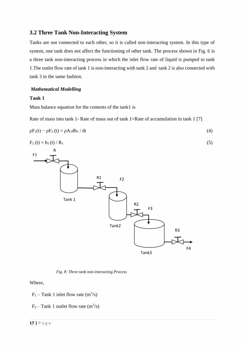
3.2 Three Tank Non-Interacting System
Tanks are not connected to each other, so it is called non-interacting system. In this type of
system, one tank does not affect the functioning of other tank. The process shown in Fig. 6 is
a three tank non-interacting process in which the inlet flow rate of liquid is pumped to tank
1.The outlet flow rate of tank 1 is non-interacting with tank 2 and tank 2 is also connected with
tank 3 in the same fashion.
Mathematical Modelling
Tank 1
Mass balance equation for the contents of the tank1 is
Rate of mass into tank 1- Rate of mass out of tank 1=Rate of accumulation in tank 1 [7]
ρF1(t) − ρF2 (t) = ρA1dh1 / dt (4)
F2 (t) = h1 (t) / R1 (5)
Fig. 8: Three tank non-interacting Process
Where,
F1 – Tank 1 inlet flow rate (m3/s)
F2 – Tank 1 outlet flow rate (m3/s)
F4
Tank 1
Tank2
Tank3
R3
F3 R2
R1 F2
F1 R

18 | P a g e
R1 - Outlet flow rate of resistance of tank1 (m/ (m3/s))
A1 - Cross-section area of tank 1 (m2)
h1 - liquid level in tank 1 (m)
ρ - density of liquid (Kg/m3)
Tank2
Mass balance equation for the contents of the tank2 is
ρF2(t) – ρF3 (t) = ρA2dh2 / dt (6)
F3 (t) = h2 (t) / R2 (7)
Where,
F2 – Tank 2 inlet flow rate (m3/s)
F3 – Tank 2 outlet flow rate (m3/s)
R2 - outlet flow rate of resistance of tank 2 (m/ (m3/s))
A2 - cross-section area of tank 2 (m2)
h2 - liquid level in tank 2 (m)
ρ - density of liquid (Kg/m3)
Tank3
Mass balance equation for the contents of the tank3 is
ρF3(t) – ρF4 (t) = ρA3dh3 / dt (8)
F3 (t) = h3 (t) / R3 (9)
Where,
F3 – Tank 3 inlet flow rate (m3/s)
F4 – Tank 3 outlet flow rate (m3/s)
R3 - outlet flow rate of resistance of tank 3 (m/ (m3/s))
A3 - cross-section area of tank 3 (m2)

19 | P a g e
h3 - liquid level in tank 3 (m)
ρ - density of liquid (Kg/m3)
The overall transfer function of three tank non-interacting process is determined using Eq. (1)
to Eq. (6) and obtained equation is
𝐻3(𝑠)
𝐹1(𝑠)=
𝑅3
(𝐴1𝑅1𝑠+1)(𝐴2𝑅2𝑠+1)(𝐴3𝑅3𝑠+1) (10)
By considering A1 =A2 =1 m2, A3 = 0.5 m2
R1=R2= 2 (m/(m3/s)), R3 = 4 (m/(m3/s)) [2];
𝐻3(𝑠)
𝐹1(𝑠)=
4
8𝑠3+12𝑠2+6𝑠+1 (11)
Using half-rule method [3], third order equation is reduced to first order with time delay
function. The above equation is reduced to
𝐻3(𝑠)
𝐹1(𝑠)=
4
3𝑠+1𝑒−3𝑠 (12)
Simulations
The three tank non-interacting process is designed and simulated using LabVIEW. The
simulation of process with the conventional PID, IMC and IMC-based PID scheme have been
shown in Fig. 10, Fig. 11 and Fig. 12 respectively.
3.3 Three Tank Interacting System and Combination of Non-Interacting
and Interacting System
Three tank system can have different combinations of interaction and no-interaction among
each other. Mainly, three combinations are discussed here.
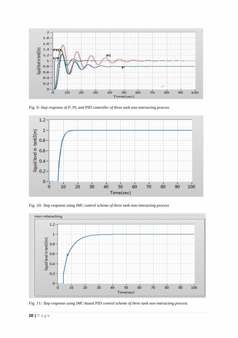
20 | P a g e
Fig. 9: Step response of P, PI, and PID controller of three tank non-interacting process
Fig. 10: Step response using IMC control scheme of three tank non-interacting process
Fig. 11: Step response using IMC-based PID control scheme of three tank non-interacting process
21 | P a g e
Tank 1 Tank2 Tank3
R3 F4
R2
R1
sahd
F1 R
F3
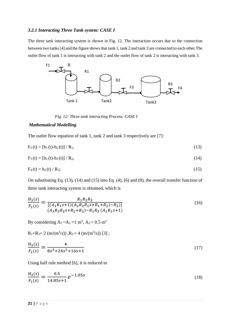
3.2.1 Interacting Three Tank system: CASE I
The three tank interacting system is shown in Fig. 12. The interaction occurs due to the connection
between two tanks [4] and the figure shows that tank 1, tank 2 and tank 3 are connected to each other.The
outlet flow of tank 1 is interacting with tank 2 and the outlet flow of tank 2 is interacting with tank 3.
Fig. 12: Three tank interacting Process: CASE I
Mathematical Modelling
The outlet flow equation of tank 1, tank 2 and tank 3 respectively are [7]:
F2 (t) = [h1 (t)-h2 (t)] / R1, (13)
F3 (t) = [h2 (t)-h3 (t)] / R2, (14)
F4 (t) = h3 (t) / R3; (15)
On substituting Eq. (13), (14) and (15) into Eq. (4), (6) and (8), the overall transfer function of
three tank interacting system is obtained, which is
𝐻3(𝑠)
𝐹1(𝑠)=
𝑅1𝑅2𝑅3
[(𝐴1𝑅1𝑠+1)(𝐴2𝑅2𝑅1𝑠+𝑅1+𝑅2)−𝑅2)](𝐴3𝑅3𝑅2𝑠+𝑅2+𝑅3)−𝑅1𝑅3 (𝐴1𝑅1𝑠+1)
(16)
By considering A1 =A2 =1 m2, A3 = 0.5 m2
R1=R2= 2 (m/(m3/s)) ,R3 = 4 (m/(m3/s)) [3] ;
𝐻3(𝑠)
𝐹1(𝑠)=
4
8𝑠3+24𝑠2+16𝑠+1 (17)
Using half rule method [6], it is reduced to
𝐻3(𝑠)
𝐹1(𝑠)=
0.5
14.85𝑠+1𝑒−1.05𝑠 (18)
22 | P a g e
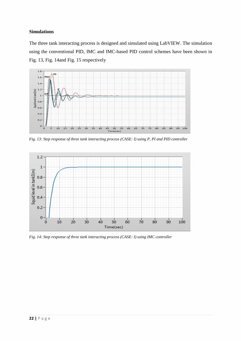
Simulations
The three tank interacting process is designed and simulated using LabVIEW. The simulation
using the conventional PID, IMC and IMC-based PID control schemes have been shown in
Fig. 13, Fig. 14and Fig. 15 respectively
Fig. 13: Step response of three tank interacting process (CASE: I) using P, PI and PID controller
Fig. 14: Step response of three tank interacting process (CASE: I) using IMC controller

23 | P a g e
Tank 1 Tank 2
Tank 3
R3 F4
R2 R1 F2
F1 R
F3
Fig. 15: Step response of three tank interacting process (CASE: I) using IMC-based PID controller
3.2.2 Three tank interacting process: CASE II
Combination of interacting and non-interacting three tank system is shown in Fig. 16.It shows
that tank 1 is interacting with tank 2 and tank 3 is non-interacting with tank 2.
Fig.16: Three tank interacting Process: CASE II
Mathematical Modelling
The outlet flow equation of tank 1, tank 2 and tank 3 respectively are [7]:
F2 (t) = [h1 (t)-h2 (t)] / R1, (19)
F3 (t) = h2 (t)/ R2, (20)
F4 (t) = h3 (t) / R3; (21)
24 | P a g e
On substituting Eq. (19), (20) and (21) into Eq. (4), (6) and (8), the overall transfer function of three
tank interacting process is obtained, which is:
𝐻3(𝑠)
𝐹1(𝑠)=
𝑅1𝑅3
[(𝐴1𝑅1𝑠+1)(𝐴2𝑅2𝑅1𝑠+𝑅1+𝑅2)−𝑅2)](𝐴3𝑅3𝑠+1)
(22)
By considering A1 =A2 =1 m2, A3 = 0.5 m2
R1=R2= 2 (m/(m3/s)) ,R3 = 4 (m/(m3/s)) [3] ;
𝐻3(𝑠)
𝐹1(𝑠)=
4
8𝑠3+16𝑠2+8𝑠+1 (23)
Using half rule method [3], it is reduced to
𝐻3(𝑠)
𝐹1(𝑠)=
0.52
6𝑠+1𝑒−1.77𝑠
(24)
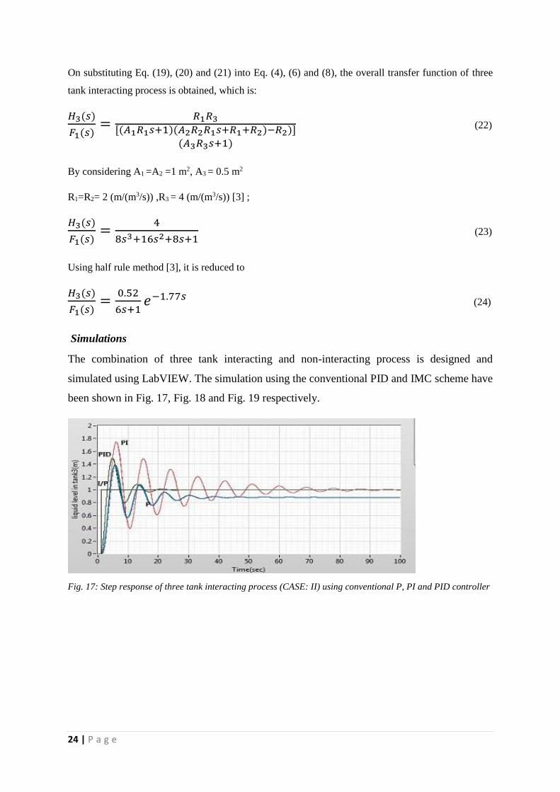
Simulations
The combination of three tank interacting and non-interacting process is designed and
simulated using LabVIEW. The simulation using the conventional PID and IMC scheme have
been shown in Fig. 17, Fig. 18 and Fig. 19 respectively.
Fig. 17: Step response of three tank interacting process (CASE: II) using conventional P, PI and PID controller

25 | P a g e
Fig. 18: Step response of three tank interacting process (CASE: II) using IMC controller.
Fig. 19: Step response of three tank interacting process (CASE: II) using IMC-based PID controller.
3.2.3 Three Tank Interacting Process: CASE III
Fig. 20 shows combination of interacting and non-interacting three tank system in which tank
1 is non-interacting with tank 2 and tank 3 is interacting with tank 2.
Mathematical Modelling
The outlet flow equation of tank1, tank2 and tank3 respectively are [7]:
F2 (t) = h1 (t)/ R1, (25)
F3 (t) = [h2 (t)-h3 (t)] / R2, (26)
F4 (t) = h3 (t) / R3; (27)

26 | P a g e
Fig.20: Three tank interacting Process: CASE III
On substituting Eq. (22), (23) and (24) into Eq. (1), (3) and (5), the overall transfer function of three
tank interacting system is obtained, which is:
𝐻3(𝑠)
𝐹1(𝑠)=
𝑅2𝑅3
((𝐴2𝑅2𝑠+1)(𝐴3𝑅2𝑅3𝑠+𝑅2+𝑅3)−𝑅3)(𝐴1𝑅1𝑠+1)
(28)
By considering A1 =A2 =1 m2, A3 = 0.5 m2
R1=R2= 2 (m/(m3/s)) ,R3 = 4 (m/(m3/s)) [6] ;
𝐻3(𝑠)
𝐹1(𝑠)=
4
8𝑠3+20𝑠2+10𝑠+1 (29)
Using half rule method it is reduced to
𝐻3(𝑠)
𝐹1(𝑠)=
0.5
8.5𝑠+1𝑒−1..53𝑠 (30)
Simulations
The combination of three tank interacting and non-interacting process is designed and
simulated using LabVIEW. The simulation using the conventional PID, IMC and IMC-based
PID scheme have been shown in Fig. 21, Fig.22 and Fig. 23 respectively.
R1 F2
Tank 1
Tank2 Tank3
R3
F4
R2
F1 R
F3

27 | P a g e
Fig. 21: Step response of three tank interacting process (CASE: III) using conventional PID controller
Fig. 22: Step response of three tank interacting process (CASE: III) using IMC controller
Fig. 23: Step response of three tank interacting process (CASE: III) using IMC-based PID controller

28 | P a g e
Result and Discussion
The overshoot and settling time of different combinations of three tank process are obtained
from simulation results and are shown in Table 10.
Table 10: Maximum overshoot and settling time of different combinations of three tank process
S.
No.
Type of Process Type of Controller Maximum
Overshoot
(in %)
Settling Time
(in sec)
1. Non-Interacting P
PI
PID
IMC
IMC-PID
24
56
40
0
0
40
65
22
18
31
2. Interacting:
CASE I
P
PI
PID
IMC
IMC-PID
50
70
56
0
0
35
42
16
17
12
3. Interacting:
CASE II
P
PI
PID
IMC
IMC-PID
38
76
48
0
0
36
68
21
26
19
4. Interacting:
CASE III
P
PI
PID
IMC
IMC-PID
52
71
43
0
0
38
50
20
13
18
The performance of the P, PI, PID controller, IMC and IMC-based PID control scheme have
been obtained using step input in LabVIEW. In Fig. 9, 13, 17, and 21, it is seen that P controller

29 | P a g e
settles faster and has lower overshoot than PI controller but has offset error. PI controller has
zero offset but has higher overshoot and settling time is also large. PID controller settles faster,
has no offset error and has low overshoot. Therefore, most of the controller used in industries
are PID controller instead of P and PI controller.
In simulation results shown in Fig. 10, 11, 14, 15, 18, 19, 22 and 23, IMC and IMC-based PID
control is depicted. It is concluded that it has zero overshoot and zero offset error. Settling time
can be decreased by increasing the filter coefficient in the controller. So, it can be maintained
according to process requirements. IMC control scheme is more complex than conventional
PID controller, so IMC is generally used in the process where overshoot is always required to
be zero, otherwise PID control is implemented due to its simplicity and easiness in handling
and tuning.

30 | P a g e
CHAPTER-4
CONCLUSIONS
4.1 Conclusions
4.2 Suggestions for Future Works

31 | P a g e
This chapter gives the conclusion of this project work and provides suggestions for future
works.
4.1 Conclusions
This project consists of analysis of different tuning methods of PID controller for different
kinds of process transfer function. Ziegler-Nichols method and Cohen-Coon methods are
implemented on different types of transfer function. Ziegler-Nichols closed loop method
cannot be implemented to any even order characteristic equation because of cancellation of
gain constant. Ziegler-Nichols open loop method is only used to FODTP or first order process
only. Higher order process cannot be controlled by Ziegler-Nichols open loop method.
IMC control has been applied on various combinations of three tank system and the results
obtained are compared with those obtained using conventional feedback controller like P, PI
and PID. The overshoot has decreased to zero as we apply IMC controller. The process
performances can be varied by varying filter coefficient of the controller. As its value is
increased, settling time and maximum overshoot decrease. It is also concluded that settling
time decreases as we go from non-interacting to interacting process using PID controller. The
settling time and maximum overshoot in three tank systems were analysed through computer
simulation using LabVIEW software package.
4.2 Suggestions for Future Works
Future scope of this project work can include
Exploring new tuning methods for perfect control of process.
Implementation of controller in industries
Designing suitable control strategy for level process.

32 | P a g e
REFERENCES
[1] B. Wayne Bequette, “Process Control: Modelling, Design and Simulation”, Prentice Hall
(2003), ISBN: 0-13-353640-8.
[2] C. A. Smith and A. B. Corripio, “Principles and Practice of Automatic Process Control”,
John Wiley & Sons, Inc., ISBN 0-47 1-88346-8.
[3] N.Khera, S. Balguvhar, and B.B.Shabarinath, “Analysis of PID Controller for Second Order
System Using NI LabVIEW”, International Journal of Emerging Technology and Advanced
Engineering, December 2011
[4] J. C. Basilio and S. R. Matos, “Design of PI and PID Controllers with Transient
Performance Specification”, IEEE Transactions on Education, vol. 45, no. 4, pp. 364-370,
November 2002.
[5] J.S Lather and Linkan Priyadarshini, “Design of IMC-PID controller for a higher order
system and its comparison with conventional PID controller,” International Journal of
Innovative Research in Electrical, Electronics, Instrumentation and Control Engineering, vol.
1, no. 3, pp. 108-112, June 2013.
[6] M.Suresh and G.J Srinivasan, “Integrated Fuzzy Logic Based Intelligent Control of Three
Tank System”, Serbian Journal of Electrical Engineering, vol. 6, no. 1,pp. 1-14, May 2009.
[7] E. Kumar and M. Sankar, “Detection of Oscillation in Three Tank Process for Interacting
and Non-Interacting cases”, International Multi-Conference in Automation, Computing,
Communication, Control and Compressed Sensing, pp. 352-357, March 2013.